Magnetic Core Losses The PSMA-Dartmouth Studies

Pilot Project

Phase II Project

A Supplemental Report

by

Edward Herbert

Co-chairman,

PSMA Magnetics Committee

December 14, 2011

Revised January 4, 2012

Sponsored by The Power Sources Manufacturers Association

email: power@psma.com http://www.psma.com/

P.O. Box 418 Mendham, NJ 07945-0418

Tel: (973) 543-9660 Fax: (973) 543-6207

2

Table of Contents Table of Contents................................................................................................................ 2

Prologue .............................................................................................................................. 6

Introduction......................................................................................................................... 7

Objective of this report: .................................................................................................. 7

Summary ......................................................................................................................... 8

The Pilot Project ........................................................................................................... 10

Objectives ................................................................................................................. 10

Off-time losses .......................................................................................................... 11

Powdered iron core ................................................................................................... 13

Skewed and symmetric wave shapes ........................................................................ 13

Noise ......................................................................................................................... 14

Phase II Project ............................................................................................................. 15

Objectives ................................................................................................................. 15

Off-time losses .......................................................................................................... 15

Expanded waveform ..................................................................................................... 16

Skewed and asymmetric wave shapes ...................................................................... 17

Hippo waveform ........................................................................................................... 17

Blocking capacitor investigation............................................................................... 18

Noise ......................................................................................................................... 19

Demagnitizing tests................................................................................................... 19

The Reports................................................................................................................... 22

Composite wave-form hypothesis............................................................................. 22

Pilot Project............................................................................................................... 22

3

Phase II Project ......................................................................................................... 22

The Data........................................................................................................................ 23

Pilot Project Data ...................................................................................................... 23

Phase II Project Data................................................................................................. 23

Using the data ........................................................................................................... 23

Wish list for future projects .......................................................................................... 24

Testing of the amorphous iron core .......................................................................... 24

Testing powdered iron cores..................................................................................... 24

Testing at higher frequencies and different waveforms............................................ 24

Testing without a blocking capacitor........................................................................ 24

Testing the effects of test rig impedance .................................................................. 24

Testing with dc bias; testing transformers with load current.................................... 24

Noise reduction, ac readings ..................................................................................... 25

Testing for equal volt-seconds .................................................................................. 25

Testing for segments in the drilled core experiment................................................. 26

Testing to avoid direct coupling to the sense winding.............................................. 26

Testing for helical flux.............................................................................................. 26

Other ......................................................................................................................... 27

Appendix A–The Reports ................................................................................................. 28

Appendix B–The Data .................................................................................................... 115

Using the data ............................................................................................................. 115

Pilot Project Data ........................................................................................................ 115

Characterization-data sub-directory........................................................................ 115

Ferrite-data and Powdered-iron-data sub-directories............................................ 116

Phase II Project Data................................................................................................... 118

4

The sets/ directory................................................................................................... 119

Added files .................................................................................................................. 121

Appendix C The Excel Tool–Viewing the Data ............................................................. 122

Using the data ......................................................................................................... 122

Source data files, .csv data...................................................................................... 122

Using The Excel Tool ................................................................................................. 123

Macros..................................................................................................................... 123

Import and Export tool............................................................................................ 123

Data files on the Calc! sheet: .................................................................................. 128

Data on the Vi!, Ii!, Flux!, Emb!, Power! and Energy! worksheets ....................... 129

Equations for the export data: ..................................................................................... 129

Miscellaneous equations on other worksheets............................................................ 131

Miscellaneous calculations on the Cmd! worksheet................................................... 132

Exporting voltages, current and flux into SPICE.................................................... 132

Appendix D-The SPICE Tool–Using SPICE to examine data ....................................... 134

Macros......................................................................................................................... 134

Import and process the data ........................................................................................ 134

Import selected data to SPICE .................................................................................... 134

Set up the Simulation.................................................................................................. 136

Appendix E The CAD Tool ............................................................................................ 138

Export to CAD ............................................................................................................ 138

Rescale, add lines and nomenclature ...................................................................... 139

Comparing traces, ................................................................................................... 140

Appendix E Off-time core loss phenomenon.................................................................. 143

Ferrite cores ................................................................................................................ 143

5

Hippo and square waveforms.................................................................................. 143

Expanded waveform ................................................................................................... 147

Powdered iron core ..................................................................................................... 149

Skew and symmetrical wave shapes ........................................................................... 150

Skewed and symmetric wave shapes ...................................................................... 150

Blocking capacitor investigation................................................................................. 153

Comparisons to a SPICE model.................................................................................. 165

Test rig influences....................................................................................................... 175

Appendix F–Expand data................................................................................................ 178

Expand data for the drilled core, mi11-1-xxx......................................................... 186

Expand data for the E core, fx05 ............................................................................ 188

Expanded data for E-core, fx09 .............................................................................. 189

Powdered iron core ................................................................................................. 190

Appendix G–Hippo data ................................................................................................. 191

Appendix H Drilled core data ......................................................................................... 202

Drilled core test sets.................................................................................................... 203

Appendix I –Simple SPICE model ................................................................................. 213

Using the model with other waveforms ...................................................................... 225

Three more examples are shown below...................................................................... 228

References....................................................................................................................... 231

Patent status ................................................................................................................ 231

6

Prologue The study of core losses began with dissatisfaction with available SPICE models for saturable cores.

A SPICE model must work with "real" parameters, volts, current, and time. This led to questioning the use of magnetic parameters for calculating core losses. For an electrical engineer, volts, seconds and amperes are much more meaningful than webers, teslas, gauss and oersteds. A simplified representation is much easier to use and avoids errors of using unfamiliar parameters and converting them.

An early hypothesis [1] was that that square wave core loss data expressed as voltage and pulse width could be used to reconstruct low duty-ratio losses. Testing this hypothesis was the premise of the Pilot Project, a study sponsored by PSMA at Dartmouth under the direction of Dr. Charles Sullivan.

The Pilot Project showed that the "composite waveform hypothesis" was an improvement both for ease of use and for accuracy. However, testing with low duty-ratio waveforms showed that it was incomplete. There were unexplained additional losses per cycle with low duty-ratio waveforms.

Dr. Sullivan presented a paper at APEC2010, Core Loss Predictions for General PWM Waveforms from a Simplified Set of Measured Data [3]

A paper by Jonas Mühlethaler, et al, Power Electronic Systems Laboratory, ETH Zurich, Switzerland, Improved Core Loss Calculation for Magnetic Components Employed in Power Electronic Systems, APEC 2011, [2] attributed the additional losses to a "relaxation process," and a method of estimating the losses was given.

The Phase II Project, sponsored by PSMA, continued the core loss study at Dartmouth. More cores were tested and a massive amount of data was taken. The added loss per cycle with low duty-ratio waveforms was confirmed. Drilled cores with sense windings explored the possibility of flux migration, with interesting but inconclusive results.

7

Introduction Objective of this report:

This supplemental report can be downloaded as a pdf document at http://www.psma.com/coreloss/supplement.pdf

This report is supplemental, and has several purposes:

1. A brief narrative describing the Pilot Project and the Phase II Project, giving the objectives, their execution and conclusions.

2. The project reports are included as Appendix A.

3. A description of the data generated. A brief description is in the report with a more complete description as Appendix B.

4. A description of the tools used for this report. A brief description is in the body of this report, with more complete descriptions in the appendices:

Appendix C, The Excel Tool

Appendix D, The SPICE Tool

Appendix E, The CAD Tool

5. Further analysis of the data. A brief description is in the body of this report, with more complete discussions in the appendices:

Appendix F, Off-time Core loss Phenomenon

Appendix G, Expand Data

Appendix H, Hippo Data

Appendix I, Drilled Core Data

Appendix J, Simple SPICE Model

6. Identify subjects for future study.

The "Wish List" for future projects is at the end of this section.

8

Summary

This report further analyzes the data from the Pilot Project, the Phase II Project and information from J. Mühlethaler's paper [2].

Key conclusions are:

1. Increased off-time does increase the energy loss per cycle, but mostly the off-time provides a window of opportunity to see and identify some loss factors while other loss factors are reduced or absent.

2. The test circuit and protocol can influence losses, including off-time losses. However, these influences are present in practical circuits as well, and they need to be identified and quantified. It is therefore not valid to dismiss them as "test rig artifacts."

3. Energy going into a magnetic core is divided between "burned energy" and "stored energy." Separating them is daunting.

a. Burned energy probably can be quantified quite well (but not entirely) using the composite waveform hypothesis.

b. Stored energy carried forward reduces the net input current and thus the input power and energy per cycle.

c. The loss of stored energy significantly influences core losses. It is attributable to the core characteristics (delayed burned energy); the external circuit (or test rig); and the test protocol (waveform).

d. Some losses may be impulses or spikes, at the switching time, and thus are analogous to switching losses.

e. Stored energy loss is particularly difficult to quantify in a simple expression. It is unlikely to be quantifiable as a material characteristic.

4. Determining the stored energy carried forward from pulse to pulse and the loss of that stored energy is essential to improving the estimation of core loss and improving circuit performance.

5. Equations such as the familiar Steinmetz equation and its many enhancements become complicated to the extent that their general use is unlikely. At least five loss mechanisms must be accounted for as well as the influences of the external circuit and waveform.

6. It must be concluded that the composite waveform hypothesis is a failure, at least as applied to high frequency core losses. That it compares well with other models is pointless if its results have large errors at low duty-ratio.

9

7. Using the "hippo" waveform to analyze core losses may be the most significant accomplishment of the Phase II project. The hippo waveform is unlikely to be used for practical power converters, but its use for analysis is brilliant.

8. The most promising way to characterize core losses may be as an impedance.

9. Characterizing a specific core or a specific wound component is better (more accurate, easier to use) than characterizing a material.

10. An impedance model can be used for improved SPICE simulations.

A working hypothesis is that if the hysteresis loop can be faithfully reproduced using an impedance model for various waveforms, the loss estimations will be as good as the match of the areas within the hysteresis loops. Because a very important factor is the stored energy and its loss, faithfully reproducing the current during the off time of low duty-ratio waveforms is important.

Impedance models are familiar turf for an electrical engineer. Measuring them is fundamental to circuit analysis. Quantifying them both in the time and frequency domain is fundamental to stability analysis. Synthesizing them is fundamental to the design of filters and compensation networks. This expertise can be applied to modeling the magnetic core. Overkill should be avoided. A simple model may suffice for most applications.

One must not lose track of the fact that a model is an analogy. It may not reveal much about the physics of what is happening in the core.

10

The Pilot Project

The Pilot Project was approved by PSMA and a purchase order to Dartmouth was issued in the Spring of 2009.

The Pilot Project was constrained by the existing test equipment and by time and budget limitations. When there is mention of things not accomplished in the Pilot Project, it emphatically is not a criticism of Dartmouth. They did an outstanding job considering the constraints and significantly advanced our understanding of core losses. Things not accomplished are mentioned only as a wish list for future projects.

Objectives

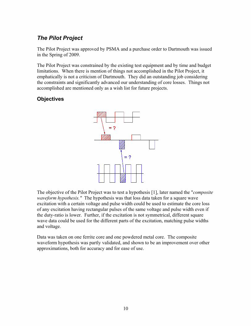
The objective of the Pilot Project was to test a hypothesis [1], later named the "composite waveform hypothesis." The hypothesis was that loss data taken for a square wave excitation with a certain voltage and pulse width could be used to estimate the core loss of any excitation having rectangular pulses of the same voltage and pulse width even if the duty-ratio is lower. Further, if the excitation is not symmetrical, different square wave data could be used for the different parts of the excitation, matching pulse widths and voltage.

Data was taken on one ferrite core and one powdered metal core. The composite waveform hypothesis was partly validated, and shown to be an improvement over other approximations, both for accuracy and for ease of use.

11

Off-time losses

With lower duty-ratio excitation, the energy per pulse was higher than in a square-wave, and the loss per pulse increased with increasing off-time.

Ferrite core

The off-time effect was more pronounced in the ferrite core. The effect was quite strong, with energy increases as much as 30 percent.

A lot of work was done taking extensive data and ensuring to the extent possible that the effect was not due to test rig anomalies.

12

Hysteresis loop

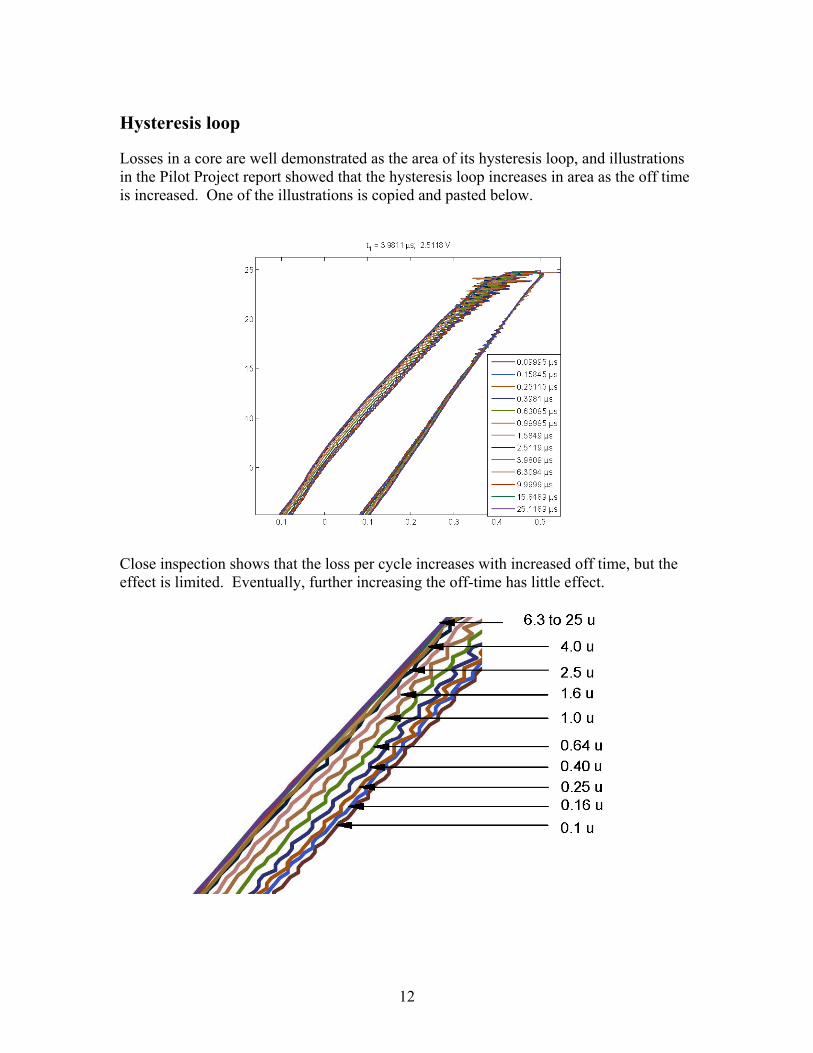
Losses in a core are well demonstrated as the area of its hysteresis loop, and illustrations in the Pilot Project report showed that the hysteresis loop increases in area as the off time is increased. One of the illustrations is copied and pasted below.

Close inspection shows that the loss per cycle increases with increased off time, but the effect is limited. Eventually, further increasing the off-time has little effect.

13

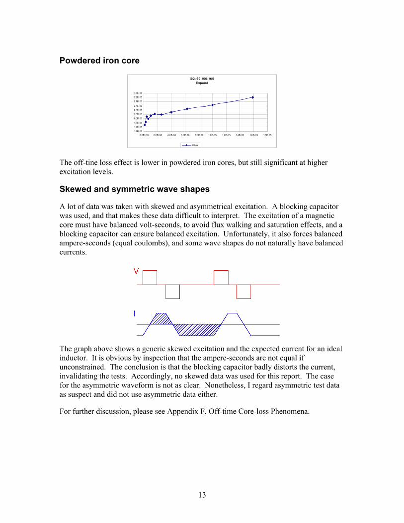
Powdered iron core

i02-60,156-165Expand

1.8E-03

1.9E-03

1.9E-03

2.0E-03

2.0E-03

2.1E-03

2.1E-03

2.2E-03

2.2E-03

2.3E-03

0.0E+00 2.0E-06 4.0E-06 6.0E-06 8.0E-06 1.0E-05 1.2E-05 1.4E-05 1.6E-05 1.8E-05

i02 ex

The off-tine loss effect is lower in powdered iron cores, but still significant at higher excitation levels.

Skewed and symmetric wave shapes

A lot of data was taken with skewed and asymmetrical excitation. A blocking capacitor was used, and that makes these data difficult to interpret. The excitation of a magnetic core must have balanced volt-seconds, to avoid flux walking and saturation effects, and a blocking capacitor can ensure balanced excitation. Unfortunately, it also forces balanced ampere-seconds (equal coulombs), and some wave shapes do not naturally have balanced currents.

The graph above shows a generic skewed excitation and the expected current for an ideal inductor. It is obvious by inspection that the ampere-seconds are not equal if unconstrained. The conclusion is that the blocking capacitor badly distorts the current, invalidating the tests. Accordingly, no skewed data was used for this report. The case for the asymmetric waveform is not as clear. Nonetheless, I regard asymmetric test data as suspect and did not use asymmetric data either.

For further discussion, please see Appendix F, Off-time Core-loss Phenomena.

14

Noise

f13-010.csv

Ringing in the current measurements is a significant problem, particularly at lower excitation levels. This reflects into the hysteresis loops and other measurements. However, the flux and energy are integrated parameters, so the ringing tends to be filtered out. As an example, the loss is represented by the area of a hysteresis loop. If a ring about a nominal value has equal area, plus and minus, the net area is unchanged. While absolute accuracy may be questioned, the qualitative results probably are valid.

f13-010.csv

15

Phase II Project

The Phase II Project was approved by PSMA and a purchase order to Dartmouth was issued in the Spring of 2010.

The Phase II Project was constrained by the existing test equipment and by time and budget constraints. When there is mention of things not accomplished in the Phase II Project, it emphatically is not a criticism of Dartmouth. They did an outstanding job considering the constraints, and significantly advanced our understanding of core losses in ferrites. Things not accomplished are mentioned only as a wish list for future projects.

Objectives

The Phase II project had two principle objectives:

1. To test the composite waveform hypothesis on a variety of cores of different materials, with emphasis on ensuring that the off-time loss phenomenon was not just a test rig or test procedure artifact.

2. To test a core that had been drilled through with sense windings installed, to see if flux migration may contribute to the off-time loss phenomenon.

Largely, the Phase II project was to confirm and expand the conclusions of the Pilot project, so very similar test protocol was used

Off-time losses

The off-time losses were confirmed for a variety of different materials. See Appendix F, Off-time Core-loss Phenomena for further details.

During excitation, energy is stored in the magnetic core as LIE *21 2=

A distinct decrease in the current is apparent after the voltage goes to 0 V, and the time constant appears to be consistent with the off-time loss phenomenon. Thus, the working hypothesis is that energy is dissipated during the off-time. The current of the stored energy superposes on the applied current, reducing the current and thus the input power and energy per cycle. This loss is less using square-wave excitation. As the off-time increases, the current decays, requiring more current, and thus more energy, in subsequent cycles.

Further confirmation is found in a paper by Jonas Mühlethaler [2], though his different time constant is unexplained.

A discussion of the off-time losses is in Appendix F, Off-time Core Loss Phenomenon.

16

Expanded waveform

There is a very good presentation of losses per cycle for expanded waveforms by material in the report. No supplement is needed for that data.

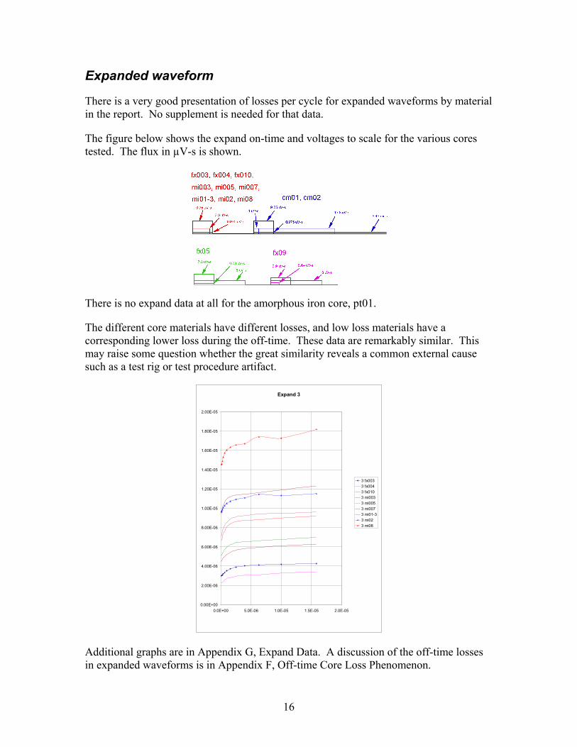
The figure below shows the expand on-time and voltages to scale for the various cores tested. The flux in µV-s is shown.

There is no expand data at all for the amorphous iron core, pt01.

The different core materials have different losses, and low loss materials have a corresponding lower loss during the off-time. These data are remarkably similar. This may raise some question whether the great similarity reveals a common external cause such as a test rig or test procedure artifact.

Expand 3

0.00E+00

2.00E-06

4.00E-06

6.00E-06

8.00E-06

1.00E-05

1.20E-05

1.40E-05

1.60E-05

1.80E-05

2.00E-05

0.0E+00 5.0E-06 1.0E-05 1.5E-05 2.0E-05

3 fx0033 fx0043 fx0103 mi0033 mi0053 mi0073 mi01-33 mi023 mi08

Additional graphs are in Appendix G, Expand Data. A discussion of the off-time losses in expanded waveforms is in Appendix F, Off-time Core Loss Phenomenon.

17

Skewed and asymmetric wave shapes

A lot of data was taken with skewed and asymmetrical excitation. A blocking capacitor was used, and that makes these data difficult to interpret. The excitation of a magnetic core must have balanced volt-seconds, to avoid flux walking and saturation effects, and a blocking capacitor can ensure balanced excitation. Unfortunately, it also forces balanced ampere-seconds (equal coulombs), and some wave shapes do not naturally have balanced currents.

The graph above shows a generic skewed excitation and the expected current for an ideal inductor. It is obvious by inspection that the ampere-seconds are not equal if unconstrained. The conclusion is that the blocking capacitor badly distorts the current, invalidating the tests. Accordingly, no skewed data was used for this report. The case for the asymmetric waveform is not as clear. Nonetheless, I regard asymmetric test data as suspect and did not use asymmetric data either.

For further discussion, please see Appendix F, Off-time Core-loss Phenomena.

See Appendix G, Expand Data.

Hippo waveform

The introduction of the "hippo" waveform may be the most important success of the Phase II project. It is unlikely to have a practical use in power converters, but its introduction as an analytical tool is brilliant.

If a positive voltage excitation pulse is immediately followed by a negative pulse of equal magnitude and pulse width, the current ideally ramps up, then ramps down the same amount, returning to 0 A, a condition where there is no stored energy and thus no residual current carried forward to the next cycle. Thus no off-time loss is expected.

The "Hippo" waveform is very useful for analysis, because it shows the magnetizing current with no energy carried forward in the first pulse, followed by an equal and opposite pulse in which the energy carried forward is maximized. For more detail, please see Appendix F, Off-time Core loss Phenomenon and Appendix H, Hippo Data.

18

Blocking capacitor investigation

A quite significant change in the energy per cycle was seen when a different blocking capacitor is used. There turned out to be a simple explanation; the temperature of the core was different. Before the cause of the difference was known, exploring the difference in loss led to a much more detailed look at the data and wide ranging speculation; some of this proved to be pivotal.

There is more discussion regarding the blocking capacitor investigation in Appendix F, Off-time Core-loss Phenomena.

Drilled core tests

One hypothesis for the off time loss was that the flux in the core might change state after the excitation is removed. With approximately zero nominal volts during the off-time, the total flux would not be expected to change significantly, but the flux could migrate within the core from one region to another. The drilled core experiments showed that while there is some flux migration, the timing is such that this hypothesis is not substantiated.

The drilled core tests were proposed to see if the flux migrated in unexpected ways as excitation was applied and after it was removed. Several possibilities were considered, generally suggesting that flux might follow one path when it is dynamic, then relax to a different path under stable conditions.

One possibility was that flux might be more diffuse dynamically, then settle to a more classical radius dependent distribution at rest. To test this hypothesis, a core was drilled through so that test windings could be inserted. Originally, it was planned to drill four holes from each direction (side to side and outside to inside). A scheme was developed to allow intersecting wires to make an internal connection. If implemented, flux change (voltage) of any of 25 cross-sectional areas could be isolated.

A vendor had promised to supply the drilled core for test, but was unable to perform, so John Harris had to make arrangements himself. Drilling proved to be much more difficult that thought, so the compromise was to drill only two holes from each direction. Time and budget constraints also prevented taking data with intersecting wires.

Another hypothesis was that the extreme angle of the winding on the core might have a transverse magnetic field, causing the flux to have a spiraling path within the core during excitation, and that it might relax to a straighter (thus shorter) path while resting. To test this, it was planned to drill two intersecting holes from the outside diameter. With linear flux, there would be no flux through this probe winding, and any sensed voltage would indicate a transverse or spiral component. Unfortunately, drilling these holes proved to be too difficult and the test was never run. Since then, some winding arrangements with no transverse component have been developed and may be considered for a future test. These include some error correcting techniques borrowed from Rogowski coils.

19

While there is some flux migration, the timing is such that this is not a likely source of the off-time core loss phenomenon. The observed flux migration may correlate with dimensional resonance as explained well in the Phase II report. As frequencies increase, dimensional resonance may become important. On the other hand, higher frequency cores probably will have smaller dimensions and better damping due to the higher losses.

Further information is in Appendix I, Drilled Core Data.

Noise

Noise in the current waveform continues to be a problem. However flux and energy are integrated parameters, so the noise tends to be filtered out, and the qualitative results probably are valid.

Demagnitizing tests

There was some concern that remnant flux might affect the test results, so some effort was made to ensure that the core was demagnetized. This is a valid concern, as remnance caused by dc bias is known to affect losses in some cores. Testing showed no difference, tending to validate the testing done without demagnitizing procedures.

Sampling errors

The sampling scheme for both the Pilot project and the Phase II project comprised 1000 samples per cycle regardless of the period. This works well for relatively short periods. As an example, with a 40 µs period, the sampling period is 40 ns.

Some test periods are as long as 2 ms, with many in the order of 1 ms. Even with a 500 µs period, the sampling period becomes 500 ns, obscuring meaningful data at the transitions.

The sampling also is a problem with low duty-ratio waveforms, especially the hippo waveform, where there are four pulses per period. With a duty-ratio of 10 percent, there are 100 samples during active excitation. With the hippo waveform, that becomes 25 samples per pulse. At 5 percent duty-ratio, it is 12.5 samples per pulse, impossible as it must be an integer.

Sampling anomalies may account for peculiar behavior at extended periods.

Composite waveform hypothesis

The composite waveform hypothesis is reported to be more accurate and easier to use than other algorithms for core losses, particularly low duty-ratio pulses. Nonetheless, errors are commonly 30 percent and as much as 50 percent. The inescapable conclusion is that it is a failure for core loss analysis, at least at high frequencies.

20

Steinmetz-like equations and their application

The Steinmetz model was developed at a time when time-independent core losses dominated. At low frequencies, given a flux density, the losses were predicted fairly well regardless of the frequency, and an added correction term for frequency made the model fit quite well over a reasonable range of interest.

A failing of the Steinmetz approach is that it requires integrated parameters, so no result is possible until the cycle is done, and there is no information about what the losses are as excitation is applied and time progresses. Substituting Volts and seconds (V-s) for flux does not alter this flaw.

The Steinmetz equations and its derivatives are fundamentally a curve fitting exercise. Any formulae that spit back the loss when the parameters are entered would do as well, and one sees other expressions such as polynomials from time to time. The more constrained the range of operation, the more successful the curve fit can be.

Like Ptolemy's algorithm for celestial motion, the model can be improved with "epicycles," then "epicycles on epicycles." We tend to forget that algorithms and models are analogies and may teach very little about what is happening physically.

For years, the Steinmetz equations were patched up by using different parameters for different frequency ranges, but still the accuracy is poor. As it is patched up more and more, the expressions get increasingly complex and the number of parameters proliferates until their use is so cumbersome as to be of little use for routing application. Like Ptolemy in view of Copernicus, Galileo and Kepler, it may be time to move on.

Even with multiple patches, the ability to adapt to different excitation waveforms is poor, especially at low duty-ratios. I see no way that it could ever capture the influence of external circuit characteristics.

Simple SPICE model

A simple SPICE model is described in Appendix J, Simple SPICE Model. A modification of the model is used in the analyses of Appendix F, Off-Time Core Loss Phenomena. The accuracy is fairly good for expanded waveforms. It fails when applied to the hippo waveform, with errors of 20 percent, which is better than the composite waveform hypothesis. The hippo waveform may be a better basis upon which to construct a model, with refinements then made for other waveforms. How that will evolve is speculation at this point.

Presently, developing a SPICE model on one waveform, then refining it on others is like playing "Whac-a-mole". However, I am confident that a protocol of test waveforms can be found that will lead to an orderly identification of model component parameters. The simple model does quite well with inductors and resistors. There is an observed high frequency effect that will very likely add an R-C network. There is some suggestion that

21

the principle inductor may be flux-level dependent, easy enough to add to a SPICE model.

As an impedance model, the SPICE model for core loss responds appropriately to different excitation as well as external circuit parameters, as long as the parasitic impedances are included.

The blocking capacitor investigation looked at an unexplained loss variation that turned out to be a temperature dependence. Without much analysis, it is easy to see in the hysteresis loop that the principle resistor has a fairly large positive temperature coefficient and the principle inductor has a fairly small negative temperature coefficient (maybe consistent with µ going to zero a the Curie temperature.

Although just a hypothesis for now, one that is not yet well developed, I think that it has great promis.

22

The Reports

Composite wave-form hypothesis User-friendly Data for Magnetic Core Loss Calculations, Edward Herbert, Canton, CT. November 10, 2008.

This document is in Appendix A, and can be downloaded at http://www.psma.com/coreloss/eh1.pdf

Pilot Project Testing Core Loss for Rectangular Waveforms, February 7, 2010 by Charles R. Sullivan and John H. Harris, Thayer School of Engineering at Dartmouth and Edward Herbert.

This document is in Appendix A, and can be downloaded at http://www.psma.com/coreloss/pilot.pdf

Phase II Project

Testing Core Loss for Rectangular Waveforms, Phase II Final Report, 21 September 2011 by Charles R. Sullivan and John H.Harris; Thayer School of Engineering at Dartmouth

This document is in Appendix A, and can be downloaded at http://www.psma.com/coreloss/phase2.pdf

Two other important documents are:

Using the PSMA Rectangular Waveform Core Loss Data, 8 August 2011, by John H.Harris, Thayer School of Engineering at Dartmouth.

This document is the user manual for the PSMA core loss data set. It explains the directory layout, file naming conventions, and file formats.

This document can be downloaded at http://www.psma.com/coreloss/use2.pdf

Measuring Core Loss for Rectangular Waveforms; Draft rev 168.53; June 18, 2011, by John H. Harris

This document goes into much more depth about the test procedures and programs used to take the data for this project.

This document can be downloaded at http://www.psma.com/coreloss/measure2.pdf

23

The Data

In general, the data is provided both as zip files, for convenient download and as expanded files, for convenient browsing.

Pilot Project Data

The data for the Pilot Project can be downloaded at http://www.psma.com/coreloss/pilot/

There are three sub-directories,

1. Characterization-data

2. Ferrite-data

3. Powdered-iron-data

The contents of the directories and files are explained in Appendix B, The Data.

Phase II Project Data

The data for the Phase II Project can be downloaded at http://www.psma.com/coreloss/phase2/

There are three sub-directories,

• Cores

• Sets

• Zips

The contents of the directories and files are explained in Appendix B, The Data

Using the data

For those who are familiar with SQLite, the database files may be useful (Phase II Project only). There is a good extension to the Firefox browser that I used to view the files. The coreloss.db file contains a number of calculated values determined using MatLab.

I preferred using the .csv files, partly because it is necessary for the Pilot Project data but mostly because I wanted to process the data for export to SPICE, and it is necessary to convert the negative times. It is easy to do that and to do other calculations in spreadsheets. An Excel Tool was developed for this purpose, as explained in Appendix C, The Excel Tool–Viewing the Data.

24

Wish list for future projects

Testing of the amorphous iron core

In the present data, there are no tests with either expanded waveforms or hippo waveforms.

Testing powdered iron cores

In the Pilot project report, it was incorrectly reported that the core loss phenomenon did not occur with powdered iron cores, so they were not included in the Phase II testing.

A closer look shows that while less, the off-time effect is present. Accordingly, powdered iron in greater variety and other cores should be added to future tests.

Testing at higher frequencies and different waveforms

This requires new test equipment.

Asymmetrical waveforms are important in practical circuits, and require voltage variation. Ideally, a fast programmable voltage source could do steps, ramps, triangles, sines and so forth.

The possibility of testing with controlled current rather than controlled voltage has been discussed. Some interesting differences might be discovered.

It is possible that test equipment from the semiconductor industry could be adapted to core testing.

Testing without a blocking capacitor

This requires new test equipment, and some provision to ensure that flux walking is not a problem

Testing the effects of test rig impedance

"Test rig artifacts" have been suggested as a problem, and test rig influences are hypothesized in this report. Until tested, this remains a hypothesis.

It probably is unwise to dismiss these effects as "test rig artifacts." The same problems may exist in real circuits, and they should be confirmed, identified and quantified.

These are further explained at the end of Appendix F, Off-time Core Loss Phenomenon.

Testing with dc bias; testing transformers with load current

This requires new test equipment.

25

Dc bias is known to increase core losses in ferrites.

Load current in a transformer may exacerbate some of the hypothesized test rig influences on core loss by increasing the voltage drops and inductive spikes.

Noise reduction, ac readings

The noise in the current readings is an obvious problem, and not being able to directly read true 0 may be a problem. Current probes have the known shortcoming that they require a loop be added and that they are slightly inductive.

A disk resistive current sense may be an improvement.

Testing for equal volt-seconds

There is a lot of testing for pulses of equal voltage and equal time with varying off time. This models a hysteretic converter with a constant voltage input and a varying load. As the load current becomes increasingly low, the discharge time stretches, but the hysteretic recharging time is fairly constant.

A much more common waveform in power electronics is that of a buck converter. The period usually is constant, but as the input voltage increases, the pulse-width decreases so as to maintain constant average voltage. Part of the composite waveform hypothesis was a proposed method of estimating the core losses under this excitation, and the Pilot Project report includes an example of that calculation. It is disappointing that time and budget constraints prevented taking data to see if these calculations are valid. The discovery of the off-time phenomena suggests that it is not, but we do not know by how much.

The effect of the off-time phenomena may be significant for buck converters.

26

Testing for segments in the drilled core experiment

There are some shortcomings in the drilled core experiments, and I hope that future testing can fill the gaps.

On the existing core, I would like to resolve the problem of the fluxes in the vertical slices not adding up correctly. I would also like to add testing of the sub-sections by using intersecting connections, as planned.

I would also like to try again to drill a core with four holes in each direction, so that 25 segments can be isolated.

Testing to avoid direct coupling to the sense winding

In making transformers, we strive for the best possible coupling between the primary and secondary, and that may use bi-filar winding, highly interleaved windings and other techniques.

In designing the sense winding for the present projects, the sense windings were located close to the drive winding for best coupling. This may have had the unfortunate effect of capturing coupling other than induction by flux change. It might be more of a problem in future tests with higher frequency.

The good correlation between the drilled core sense windings (at least the horizontal windings) and the overall sense windings suggests that this was not a problem. Some differences at the leading edge are suggestive that there might be a difference, but it is hard to distinguish from noise.

One idea is to use a sense winding that does not share factors with the drive winding, such as 5 turns and 13 turns. There may be other methods as well.

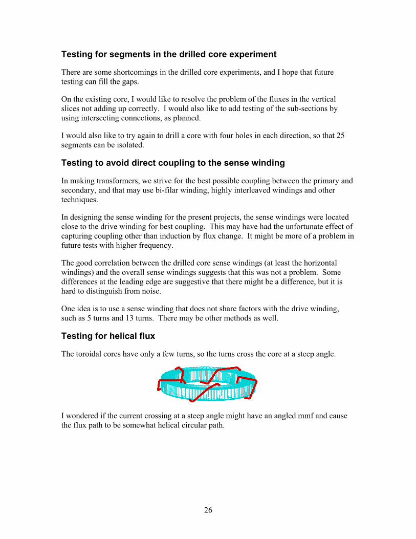
Testing for helical flux

The toroidal cores have only a few turns, so the turns cross the core at a steep angle.

I wondered if the current crossing at a steep angle might have an angled mmf and cause the flux path to be somewhat helical circular path.

27

A helical path, being somewhat longer, would have longer length and less effective area. Upon removal of the excitation, it might relax to a normal circular path with shorter length and greater area. Such a path would have higher inductance.

There are two possible explanations for a current reduction. The obvious one is losses, but another is conservation of energy with increased inductance.

E = ½ I2*L

If L goes up, I must go down correspondingly to conserve energy. Of course, both could be happening, and L might go up for reasons that have nothing to do with helical flux paths.

This test could not be done as originally planned because it required two extra holes to be drilled in the core. Drilling proved to be much more difficult than anticipated, and this plan had to be scrapped.

There are other ways to test this idea involving winding modifications, and maybe borrowing some error correcting techniques from Rogowski coils.

Other

Other ideas will occur to me and will be added in later revisions. Others are encouraged to add to this list as well.

28

Appendix A–The Reports User-friendly Data for Magnetic Core Loss Calculations, Edward Herbert, Canton, CT. November 10, 2008.

The Pilot Project Report

The Phase II Project Report

1

Introduction:

Everyone "knows" that core losses depend only upon B

)and frequency. It

does not matter what the excitation level and duty-cycle is, only the maximum flux density B

). That is true, if the

switching frequency is below 10 kHz or so. At the frequencies used in today's pulse-width-modulated (pwm) transformers, the core losses increase dramatically for low duty-cycles, as much as 10 times at 10 % duty-cycle.

Graphs of magnetic core loss data are usually for sine-wave excitation and presented in terms of maximum flux density B

)and frequency f. These graphs

are of questionable value for pulse-width-modulated (pwm) power converter design and decidedly not user-friendly. Graphs of core loss data for square-wave excitation, presented in terms of applied voltage and time are much more relevant to pwm power converter design and are much easier to use.

Background:

Magnetic core loss graphs from manufacturers are marginally useful for pwm power converter design. (1) They usually present loss in terms of maximum flux density B

), an unfamiliar

parameter of little use to the power converter designer. (2) The magnetic units used for core loss graphs are confusing and inconsistent. The likelihood of making errors is significant. (3) The graphs are for sine-wave excitation. Most pwm converters

operate with square-waves having a variable duty-cycle. (4) The graphs are notoriously inaccurate. It is not unusual to see ruler-straight lines on core loss curves, with gross inaccuracies at the extremes.

Some very interesting work has been done exploring losses at increased "effective frequency." [1], [2] and [3].

Using volt-second graphs

Figure 1 shows representative core loss curves for square-wave excitation, presented as a family of constant voltage curves vs. pulse-width t.

Figure 1: Representative core loss curves for constant voltage square-wave excitation vs. pulse-width.

User-friendly Data for Magnetic Core Loss Calculations Edward Herbert, Canton, CT. November 10, 2008

2

For a graph for a magnetic material, material, the voltage is normalized and has units of volts per area-turn and the loss is in watts per volume. Core loss graphs for specific cores can include the geometric parameters, so the units are volts/turn and watts.

Low duty-cycle data

Figure 2. Curves of constant average voltage can be plotted. Note the extreme change in slope for short pulse widths (high frequency).

In figure 2, curves of constant average voltage equal to 0.5 V were plotted for several frequencies. As an example, using the technique for low duty-cycles presented below, start with the 0.5 V line and 0.01 ms, point A. That is the loss for a square wave with 0.01 ms pulse width. At 0.001 ms, to have the same average voltage, the voltage during the pulse is 5.0 V, point B, reduced by the duty-cycle 0.1, point C. The line A-C is approximately the line showing the loss for constant average voltage. This may be the most useful curve of all for a power converter designer.

The same technique is repeated to estimate the losses at constant average voltage for other starting pulse-widths (frequencies), resulting in a family of curves, shown in figure 2.

Note that at short pulse-widths (high frequency), the losses rise significantly at low duty-cycle. At longer pulse-widths, (low frequency), the duty-cycle does not much affect losses. This latter case is the classic loss characteristic taught for magnetic design.

The reader is advised that these curves were derived using Steinmetz equations applied far beyond their limits of reasonable accuracy, using many complex manipulations, each an opportunity for error. Accordingly, the graphs are qualitative at best.

However, the graphs represent a suggested form to use for plotting "real" data, from laboratory test and measurement. Real data from real tests will always trump manipulated data and approximations.

This presentation of the data is user-friendly and much more meaningful for power converter design.

Figure 3: Times and duty-cycles defined.

3

Calculations

See figure 3 to define pulse-width and duty-cycle: In all cases, the pulses are repetitive steady-state pulses, as would be generated in a pwm converter at stead-state conditions.

For a square-wave excitation, t is the pulse-width and T is the period. The duty-cycle D is 1.0. To calculate the core losses using figure 1 for a 1 volt square-wave with a pulse-width of 2 us, follow the dashed line up from 2 us to intercept the 1 volt curve, then horizontally to intercept the vertical axis. The result is about 1.8 mw/cm3.

For a symmetrical pulsed excitation, t is the pulse-width and T is the period. The duty-cycle D is 2 * t / T. To calculate the core loss for a 1 volt pwm wave-form having a 1 volt excitation and a 2 us pulse-width and a duty-cycle of 0.5, follow the dashed line up from 2 us to intercept the 1 volt curve, then horizontally to intercept the vertical axis. The result is multiplied by the duty-cycle 0.5 to give about 0.9 mw/cm3.

For an asymmetrical pulsed excitation, the volt-seconds none-the-less must be equal for the pulses. T is the period, t1 is the positive pulse-width, t2 is the negative pulse-width. Two duty-cycles are defined, D1 = t1 / T and D2 = t2 / T.

To calculate the core loss for an asymmetrical pwm having a period of 8 us, and having a 2 us positive pulse of 1 volt and a 4 us negative pulse of 0.5 volt, first follow the dashed line up from 2 us to intercept the 1 volt curve, then horizontally to intercept the vertical axis. The result is multiplied by the duty-cycle of 0.25 to give about 0.45 mw/cm3.

Next, follow the dashed line up from 4 us to intercept the 0.5 volt curve, then horizontally to intercept the vertical axis. The result is multiplied by the duty-cycle of 0.5 to give about 0.24 mw/cm3. Add the partial results. The core loss is about 0.69 mw/cm3.

Thus a method of calculating core loss is presented that does not require calculating magnetic parameters. This data and the calculations are much more relevant to power converter design, and much more user-friendly.

Saturation

Following the constant voltage curves from left to right, the volt-seconds of each point is the product of the voltage and the pulse-width. The curve ends at the volts-seconds where the core saturates. Accordingly, as long as the voltage and pulse-widths of interest are on the curve, the core will not saturate (if there is no flux walking.)

Loss data for cores and wound components

Figure 4. For a specific core, the geometric parameters can be included, so the result is read directly as watts W.

Losses for cores: A manufacturer of magnetic cores can present data for any specific core with all of the geometric

4

parameters included, so the user need not be concerned with effective area, effective volume and the like. Knowing the volts/turn and the pulse-widths of interest, the losses in the core can be read directly from the graph, as seen in Figure 4.

Losses for wound components: A similar graphical presentation includes the turns, allowing a designer to determine the core losses directly using only the voltage and pulse-widths.

"Remagnetization velocity"

Many papers have suggested that dB/dt and B are more relevant to core loss, leading to improved methods of calculation that have a better match to test data. None, as far as we know, has recognized dB/dt as voltage (with a scale factor). Yet, for most power converter designers, voltage is a much easier parameter to use and understand.

All continue to use maximum flux density B

) and frequency f. [1] uses the

term "remagnetization velocity" for dB/dt. In [2] and [3], the more straightforward "dB/dt" is used.

For any expression using the flux density B or the maximum flux density B

), an

equivalent expression can be written substituting volt-seconds, with an appropriate scale factor.

"Effective frequency"

[1], [2] and [3] all use the concept of "effective frequency" to account for non-sinusoidal wave-forms. Intuitively, there is a relationship between "duty-cycle" and "effective frequency," duty-cycle being analogous to the ratio of the real frequency to the effective frequency.

For any expression using frequency, an equivalent expression can substitute the inverse of the period, noting that frequency f equals 1 / T, where T is the period. We prefer using the half-cycle period t, so f equals 1 / 2 t.

Steinmetz equation using voltage v and the period T

The Steinmetz equation (or any other expression using B

) and f) can be

expressed in terms of voltage and time.

βα BfCP mv

)**=

Substituting f = 1 / T and B

) = k * v * T gives

)(**

)**(*1*

αββ

βα

−′=

⎟⎠⎞

⎜⎝⎛=

TvCP

TvkT

CP

mv

mv

[T is the period, k is the scale factor converting volt-seconds to B

), v is the

voltage density and C'm = Cm * kβ.]

This exercise is to demonstrate the equivalence of the expressions, not to suggest converting present data to the new format, particularly as we prefer using square-wave excitation. New data should be taken using voltage and pulse-width.

Graphs using converted data

To illustrate the point, we converted data mathematically to make the graphs that follow.

The starting point is the data as they are usually presented for Magnetics, Inc. F material. These data were chosen because Magnetics, Inc. also provides a family of Steinmetz constants for the F

5

material, as shown in the box below [6]. The frequency ranges are colored and correspond with the colors of the curves in the graphs.

Figure 5 shows a composite graph, taking the data for the F material from a data sheet (the solid lines) and superimposing on it the curves resulting from the Steinmetz calculations (the dashed lines).

Figure 5: Core loss data for Magnetics, Inc. material F. The solid lines are from the datasheet, and the dashed lines are calculated using the Steinmetz equations.

Magnetics, Inc.'s loss expression approximation is:

dcL BfaP ˆ**= mW/cm3

[Where a, c and d are constants, f is in kHz and B is in kG.]

For each line in figure 3, the slope of the line is the exponent d, and the spacing between the lines is governed by the exponent c.

Core loss vs. frequency.

Figure 6: The data for Magnetics Inc. material F was re-plotted as a family of curves of constant flux density vs. frequency.

For Magnetics Inc.'s F material, the Steinmetz constants are given as follows.

Range a c d

f ≤ 10 kHz 0.790 1.06 2.85 10 kHz ≤ f < 100 kHz 0.0717 1.72 2.66 100 kHz ≤ f < 500 kHz 0.0573 1.66 2.68 f ≥500 kHz 0.0126 1.88 2.29

The colors correspond to frequency ranges in the graphs.

6

First, the data was re-plotted using curves of constant B vs. f as in figure 6. Note the extreme discontinuities in the calculated data (dashed lines). These lines should be continuous, pointing out dramatically how poor the Steinmetz approximation is at the extremes of the frequency ranges. The solid lines are drawn free-hand in an attempt to find the best fit through the calculated data.

Excitation voltage vs. frequency

Figure 7: The data are re-plotted as a family of curves of constant excitation vs. frequency.

Next, the data is plotted in terms of voltage and frequency This required substituting volt-seconds (with a scale factor) for B , but then substituting back the frequency f term as the inverse of the seconds. The result is a family of loss curves of the excitation voltage (in volts/turn-cm2) vs. frequency, as shown figure 7.

Again, the dashed lines are the calculated curves, and the solid lines are a "best fit" drawn free-hand. On the upper left, the lines were ended at a flux density of 3 kG. This would be a straight line if the equations were ideal.

Voltage vs. pulse-width

The final translation is to re-plot the curves in terms of pulse-width rather than frequency. Because the pulse-width t is used instead of the period T, the scale was shifted left by 2. Only the "best fit" curves were used. The graph in figure 8 was rescaled to square up the log-log coordinates, and possible asymptotes of the curves were added. With further editing for appearance, this graph became the graph of figure 1.

Figure 8: The curves of figure 7 were flipped left to right to invert the frequency scale to a time scale, and it was shifted left by 2 so that the scale is pulse-width t rather than the period T.

While this graph was derived from data for the Magnetics, Inc. F material, the reader is reminded that curves are based upon the Steinmetz equations applied far beyond their range of reasonable accuracy. The complexity of the calculations makes the chance of error quite significant. As such, only qualitative relationships can be inferred.

However, new data taken using square-wave constant voltage excitation and presented as a function of the pulse-width (half period) of the square-wave

7

will be no less accurate and valid than the data presently used, while being much more relevant to power converter design and much more "user-friendly."

Stienmetz-like equations

Rather than try to shoe-horn the Steinmetz factors into a new form, it is suggested that a new Steinmetz-like equation be defined.

εδ tvCP xv **=

Find the area on the graph over which the circuit of interest will operate, and pick three points that bracket that area. For each, write the Steinmetz-like equation, with the constants as unknowns, and solve the equations simultaneously. Since solving simultaneous equations in which two of the unknowns are exponents is daunting, it is suggested to use a math program such as MathCad.

Oliver-like equations and Ridley-Nace-like equations

In [4], Christopher Oliver presents a curve fitting algorithm that is accurate over a much broader area of the graph. In [5], Dr. Ray Ridley and Art Nace do the same (but with a much different algorithm), and introduce temperature compensation as well. We see no reason why similar techniques could not be applied to voltage and pulse-width graphs as well, as the underlying physics is the same.

Conclusion

Core loss data can be taken for square-wave excitation, and presented in terms

of the excitation voltage and pulse-width with no loss in accuracy.

Core loss data can also be taken and presented as curves of constant average voltage vs. pulse width, to show the consequence of low duty-cycle operation.

The resulting data are much more relevant to pwm power converter design, and are much more "user-friendly".

References

[1] Ansgar Brockmeyer, Manfred Albach, and Thomas Dürbaum, Remagnetization Losses of Ferrite Materials used in Power Electronic Applications, Power Conversion, May 1996 Proceedings.

[2] Jeili Li, Tarek Abdallah and Charles R. Sullivan, Improved Calculation of Core Loss with Nonsinusoidal Waveforms, IAS 2001.

[3] Kapil Venkatachalam, Charles R. Sullivan, Tared Abdallah and Hernán Tacca, Accurate Prediction of Ferrite Core Loss with Nonsinusoidal Waveforms Using Only Steinmetz Parameters, COMPEL 2002

[4] Christopher Oliver, A new Core Loss Model, Switching Power Magazine, Spring 2002.

[5] Dr. Ray Ridley and Art Nace, Modeling Ferrite Core Losses, Switching Power Magazine © Copyright 2006.

[6] Magnetics, Inc. Ferrite Cores Design Manual and Catalog, 2006.

rev 9a i

SummaryIn this project we have explored the feasibility of a method to generalize square-wavecore-loss data to predict core loss with any common rectangular voltage waveform,proposed by Herbert [1].

The hypotheses to be tested is that, for rectangular pulses and a given magnetic corematerial, the core loss energy per period depends only on component pulse widths andpeak voltages. We call this the composite waveform hypothesis. It has great intuitiveappeal, and if true, it makes it convenient to decompose rectangular waveforms intosuch pulses for analysis. Thus, it would be be sufficient to test cores with squarevoltage waveforms, and then use the data to predict losses with generalized rectangularvoltage waveforms.

Two important objectives of the project are to

1. Gather such square wave data for two typical core materials, one ferrite and onepowdered-iron.

2. Gather additional data to determine if the composite waveform hypothesis isvalid.

The square wave data were gathered for a set of data points at intervals that wouldbe practical for manufacturers to provide for designers—five values per decade for bothpeak voltage and pulse width.

The validation data were measurements for non-square-wave composites of “stan-dard” pulses from the square wave data set. We used three variations: (1) symmet-ric waveforms formed from a standard pulse shape with varying amounts of off-timeadded, increasing the period, (2) families of standard pulse shapes with set off-time,but varying the asymmetry, and (3) asymmetric waveforms with no off time, formedfrom two different standard pulse shapes.

It was clear from the large size of the sample space implied by this program, that anautomated data gathering system would be needed, so computer control was designedin from the start. A data management system evolved that can generate a set of controlinput parameters for the test setup for all data points from a few global parameters, andthen analyze the results.

The drive circuitry was designed to cover a wide range of flux density and fre-quency, consistent with budget constraints, by using existing experimental circuit boards.

The results indicate that the composite waveform hypothesis, while not perfect,performs well, and should be a significant improvement over the use of sinusoidaldata for PWM design. The deviations from composite waveform model may providevaluable insight into the loss processes, and future work to characterize this behaviorcan likely improve the model and its value for design.

ii

Contents1 Introduction 1

2 Previous Methods for Core Loss withNon-sinusoidal Waveforms 1

3 Calculating Core Loss from aSimplified Data Set 3

4 Measurement System 44.1 Data Flow . . . . . . . . . . . . . . . . . . . . . . . . . . . . . . . . 64.2 Preferred Values . . . . . . . . . . . . . . . . . . . . . . . . . . . . . 7

5 Experimental Results 85.1 Characterization . . . . . . . . . . . . . . . . . . . . . . . . . . . . . 85.2 Verification . . . . . . . . . . . . . . . . . . . . . . . . . . . . . . . 9

6 Hysteresis Loops 16

7 Design Techniques 17

8 Discussion 21

9 Using the Data 22

10 Conclusion 22

A Data Files and Fields 24A.1 Oscilloscope Data . . . . . . . . . . . . . . . . . . . . . . . . . . . . 24A.2 Test Input Data . . . . . . . . . . . . . . . . . . . . . . . . . . . . . 25A.3 Run Data Generator . . . . . . . . . . . . . . . . . . . . . . . . . . . 26

B General File Formats 27

rev 9a iii

List of Figures1 Waveform types. . . . . . . . . . . . . . . . . . . . . . . . . . . . . 32 Full-bridge excitation circuit. . . . . . . . . . . . . . . . . . . . . . . 53 Decoding waveforms. . . . . . . . . . . . . . . . . . . . . . . . . . . 54 Block diagram of the experimental apparatus. . . . . . . . . . . . . . 75 Experiment data flow. . . . . . . . . . . . . . . . . . . . . . . . . . . 86 Square-wave loss data, ferrite core. . . . . . . . . . . . . . . . . . . . 107 Square-wave loss data, powdered-iron core. . . . . . . . . . . . . . . 118 Losses with asymmetric waveforms. . . . . . . . . . . . . . . . . . . 129 Test data for waveform with off time, ferrite core. . . . . . . . . . . . 1310 Test data for waveform with off time, powdered iron core. . . . . . . . 1411 Hysteresis plots for expand data set, t1 = 3.98 µs. . . . . . . . . . . . 1512 Hysteresis plots for expand data set, t1 = 6.31 µs . . . . . . . . . . . 1613 Hysteresis plots for expand data set, t1 = 10 µs . . . . . . . . . . . . 1714 Zoomed in hysteresis plots for expand data set, t1 = 3.98 µs. . . . . . 1815 Reading a Herbert plot. . . . . . . . . . . . . . . . . . . . . . . . . . 1916 Design example. . . . . . . . . . . . . . . . . . . . . . . . . . . . . 20

List of Tables1 Devices for the Drive Circuitry. . . . . . . . . . . . . . . . . . . . . . 62 Sample cores. . . . . . . . . . . . . . . . . . . . . . . . . . . . . . . 83 File naming conventions for parameter and data files. . . . . . . . . . 244 Waveform type designations . . . . . . . . . . . . . . . . . . . . . . 25

iv

PrefaceMost of the content of this report was taken from a paper to be published in the pro-ceeding of the IEEE Applied Power Electronics Conference for 2010. I have addedmore detailed information the help with a practical understanding of the data gatheringsystem and the use of the data.

John H. Harris

rev 9a 1

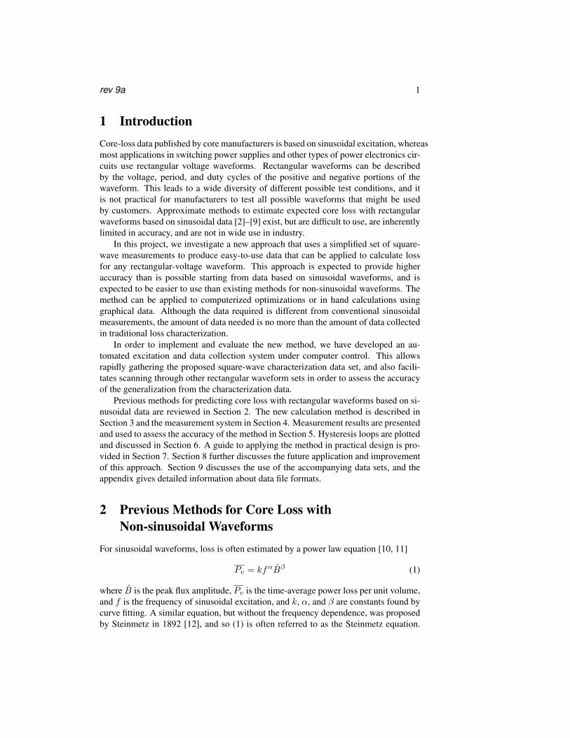
1 IntroductionCore-loss data published by core manufacturers is based on sinusoidal excitation, whereasmost applications in switching power supplies and other types of power electronics cir-cuits use rectangular voltage waveforms. Rectangular waveforms can be describedby the voltage, period, and duty cycles of the positive and negative portions of thewaveform. This leads to a wide diversity of different possible test conditions, and itis not practical for manufacturers to test all possible waveforms that might be usedby customers. Approximate methods to estimate expected core loss with rectangularwaveforms based on sinusoidal data [2]–[9] exist, but are difficult to use, are inherentlylimited in accuracy, and are not in wide use in industry.

In this project, we investigate a new approach that uses a simplified set of square-wave measurements to produce easy-to-use data that can be applied to calculate lossfor any rectangular-voltage waveform. This approach is expected to provide higheraccuracy than is possible starting from data based on sinusoidal waveforms, and isexpected to be easier to use than existing methods for non-sinusoidal waveforms. Themethod can be applied to computerized optimizations or in hand calculations usinggraphical data. Although the data required is different from conventional sinusoidalmeasurements, the amount of data needed is no more than the amount of data collectedin traditional loss characterization.

In order to implement and evaluate the new method, we have developed an au-tomated excitation and data collection system under computer control. This allowsrapidly gathering the proposed square-wave characterization data set, and also facili-tates scanning through other rectangular waveform sets in order to assess the accuracyof the generalization from the characterization data.

Previous methods for predicting core loss with rectangular waveforms based on si-nusoidal data are reviewed in Section 2. The new calculation method is described inSection 3 and the measurement system in Section 4. Measurement results are presentedand used to assess the accuracy of the method in Section 5. Hysteresis loops are plottedand discussed in Section 6. A guide to applying the method in practical design is pro-vided in Section 7. Section 8 further discusses the future application and improvementof this approach. Section 9 discusses the use of the accompanying data sets, and theappendix gives detailed information about data file formats.

2 Previous Methods for Core Loss withNon-sinusoidal Waveforms

For sinusoidal waveforms, loss is often estimated by a power law equation [10, 11]

Pv = kfαBβ (1)

where B is the peak flux amplitude, Pv is the time-average power loss per unit volume,and f is the frequency of sinusoidal excitation, and k, α, and β are constants found bycurve fitting. A similar equation, but without the frequency dependence, was proposedby Steinmetz in 1892 [12], and so (1) is often referred to as the Steinmetz equation.

2

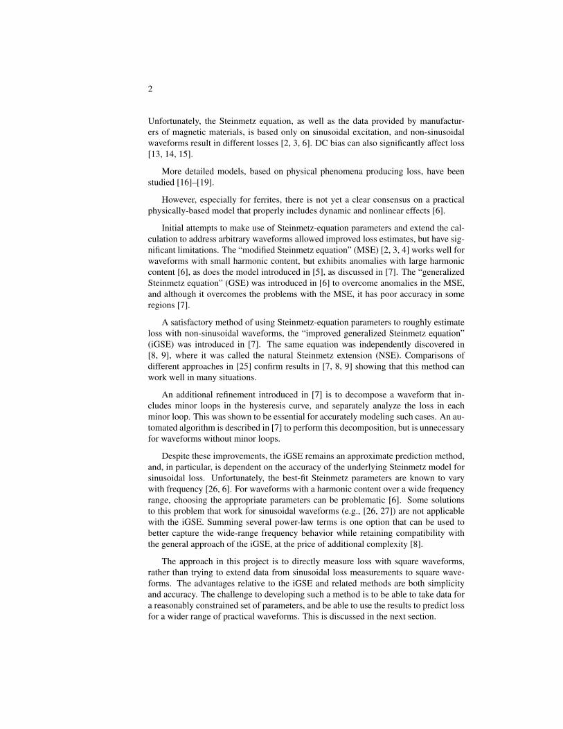
Unfortunately, the Steinmetz equation, as well as the data provided by manufactur-ers of magnetic materials, is based only on sinusoidal excitation, and non-sinusoidalwaveforms result in different losses [2, 3, 6]. DC bias can also significantly affect loss[13, 14, 15].

More detailed models, based on physical phenomena producing loss, have beenstudied [16]–[19].

However, especially for ferrites, there is not yet a clear consensus on a practicalphysically-based model that properly includes dynamic and nonlinear effects [6].

Initial attempts to make use of Steinmetz-equation parameters and extend the cal-culation to address arbitrary waveforms allowed improved loss estimates, but have sig-nificant limitations. The “modified Steinmetz equation” (MSE) [2, 3, 4] works well forwaveforms with small harmonic content, but exhibits anomalies with large harmoniccontent [6], as does the model introduced in [5], as discussed in [7]. The “generalizedSteinmetz equation” (GSE) was introduced in [6] to overcome anomalies in the MSE,and although it overcomes the problems with the MSE, it has poor accuracy in someregions [7].

A satisfactory method of using Steinmetz-equation parameters to roughly estimateloss with non-sinusoidal waveforms, the “improved generalized Steinmetz equation”(iGSE) was introduced in [7]. The same equation was independently discovered in[8, 9], where it was called the natural Steinmetz extension (NSE). Comparisons ofdifferent approaches in [25] confirm results in [7, 8, 9] showing that this method canwork well in many situations.

An additional refinement introduced in [7] is to decompose a waveform that in-cludes minor loops in the hysteresis curve, and separately analyze the loss in eachminor loop. This was shown to be essential for accurately modeling such cases. An au-tomated algorithm is described in [7] to perform this decomposition, but is unnecessaryfor waveforms without minor loops.

Despite these improvements, the iGSE remains an approximate prediction method,and, in particular, is dependent on the accuracy of the underlying Steinmetz model forsinusoidal loss. Unfortunately, the best-fit Steinmetz parameters are known to varywith frequency [26, 6]. For waveforms with a harmonic content over a wide frequencyrange, choosing the appropriate parameters can be problematic [6]. Some solutionsto this problem that work for sinusoidal waveforms (e.g., [26, 27]) are not applicablewith the iGSE. Summing several power-law terms is one option that can be used tobetter capture the wide-range frequency behavior while retaining compatibility withthe general approach of the iGSE, at the price of additional complexity [8].

The approach in this project is to directly measure loss with square waveforms,rather than trying to extend data from sinusoidal loss measurements to square wave-forms. The advantages relative to the iGSE and related methods are both simplicityand accuracy. The challenge to developing such a method is to be able to take data fora reasonably constrained set of parameters, and be able to use the results to predict lossfor a wider range of practical waveforms. This is discussed in the next section.

rev 9a 3

T

V

V

1

2

t2t1 t0

(a) Waveform parameter definitions

Shifted, D < 1

Asymmetric, D = 1

Symmetric, D < 1

Square

(b) Test waveform types

Figure 1: Waveforms (voltage vs. time): parameters and test waveform types. Squarewaves are used for characterizing materials; the other test waveforms are used to testthe validity of the composite waveform hypothesis.

3 Calculating Core Loss from aSimplified Data Set

Consider a core with voltage waveforms such as those shown in Figure 1, typical ofpower electronics applications, applied to a winding. The flux in the core will ramp upor down during each positive or negative voltage pulse, respectively. We hypothesizethat the energy loss incurred during each of these flux transitions depends only onthe amplitude and duration of the pulse, and that there is no loss during periods ofzero applied voltage (constant flux). If this is the case, we can decompose any of therectangular waveform types shown in Figure 1b into a set of two pulses, calculate theenergy loss associated with each pulse, and sum them to find the total energy loss percycle. We call this hypothesis the composite waveform hypothesis.

If the composite waveform hypothesis proves to be a good approximation, we canpredict core loss for any of the waveforms in Figure 1b if we know the loss for a squarepulse as a function of its amplitude and duration. While we might estimate that loss

4

from sinusoidal data using one of the methods describe in Section 2 ([2]–[9]), a moreaccurate approach is to collect measured test data with square voltage waveforms, forwhich we can assume that the loss associated with each pulse is one half of the per-cycle energy loss. This requires data as a function of two parameters, such as fluxamplitude and frequency, as used in conventional sinusoidal loss characterization. Theparameters may also be described in terms of applied voltage per turn (correspondingto flux ramp rate) and on-time t1 (one half the period for square waves).

The method we propose starts with characterizing a core material by measuringloss data for square waveforms. One half of the measured energy loss per cycle is theenergy lost for a single pulse of the applied amplitude and on-time. If the compositewaveform hypothesis is accurate, the same loss per cycle will be incurred for that ap-plied voltage and on-time in any composite waveform. For the waveforms we considerhere (Figure 1), the waveform comprises two pulses. To find the total energy loss percycle one sums the per-pulse loss data for each of the two sets of pulse parameters(amplitude and on-time) from the corresponding square-wave measurements.

In Sections 4 and 5 we report on experimental measurements conducted for twopurposes: (1) to collect square-wave data for sample cores as is necessary for thismethod, and (2) to assess the accuracy of the method and of the composite waveformhypothesis. We note that all of the previous methods for predicting loss with non-sinusoidal waveforms discussed in Section 2 depend on some version of the compositewaveform hypothesis, even though this assumption is rarely stated. Thus, tests of thishypothesis are important for other approaches to predicting non-sinusoidal losses aswell as for validating the approach proposed here.

Predictive core loss models built up from fundamental physical principals are notavailable for most core loss mechanisms, and so theoretical analysis of the compos-ite waveform hypothesis is not possible. However, for core loss produced purely byclassical eddy-current effects, physical models are well established, and analytical so-lutions exist for some geometries. It can be shown that, for classical eddy-current lossin core material layers thicker than or comparable to an electromagnetic skin depth,the composite waveform does not always hold exactly. However, it may still be a use-ful approximation, and may hold exactly for other types of losses. Thus experimentalevaluation is needed to assess its utility.

4 Measurement SystemWe use a two-winding loss measurement [9] on toroidal core samples with 5 or 21turns to match core characteristics to our drive system capabilities. The drive windingis connected to a full-bridge switching network through a 320 µF blocking capacitor(Figure 2). The gates of the four MOSFETs are controlled by an Agilent 33220A ar-bitrary waveform generator through a logic circuit and optically isolated gate drivers.Both the arbitrary function generator and the DC power supply feeding the bridge cir-cuit are automatically controlled by a computer to allow synthesis of a sequence ofdifferent rectangular voltage waveforms. The principle components used in the circuitare summarized in Table 1.

The Agilent waveform generator has only one arbitrary waveform output (labeled

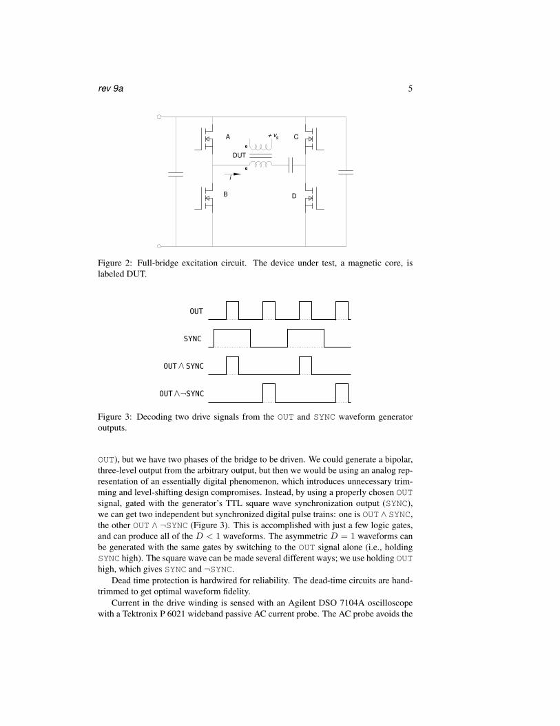
rev 9a 5

A

B D

C

DUT

i

+ vs

Figure 2: Full-bridge excitation circuit. The device under test, a magnetic core, islabeled DUT.

OUT

SYNC

OUT SYNC

OUT SYNC

Figure 3: Decoding two drive signals from the OUT and SYNC waveform generatoroutputs.

OUT), but we have two phases of the bridge to be driven. We could generate a bipolar,three-level output from the arbitrary output, but then we would be using an analog rep-resentation of an essentially digital phenomenon, which introduces unnecessary trim-ming and level-shifting design compromises. Instead, by using a properly chosen OUTsignal, gated with the generator’s TTL square wave synchronization output (SYNC),we can get two independent but synchronized digital pulse trains: one is OUT∧ SYNC,the other OUT ∧ ¬SYNC (Figure 3). This is accomplished with just a few logic gates,and can produce all of the D < 1 waveforms. The asymmetric D = 1 waveforms canbe generated with the same gates by switching to the OUT signal alone (i.e., holdingSYNC high). The square wave can be made several different ways; we use holding OUThigh, which gives SYNC and ¬SYNC.

Dead time protection is hardwired for reliability. The dead-time circuits are hand-trimmed to get optimal waveform fidelity.

Current in the drive winding is sensed with an Agilent DSO 7104A oscilloscopewith a Tektronix P 6021 wideband passive AC current probe. The AC probe avoids the

6

Table 1: Devices for the Drive Circuitry.

Function Description ValuePower supply. Sorenson XG33-25 33V, 25ASwitching MOSFET. IR IRF 3706 20V, 77AOpto-isolated gate drive. Avago HCPL-3180 2.5 A, 250 kHzBlocking capacitor. AVX FFV3 2× 160 µFPower supply decoupling capacitor,high capacity.

electrolytic 2× 120mF

Power supply decoupling capaci-tors, low Z.

X7S surface mount 10× 10 µF

delay inherent in an active current probe; delay measurements verify that the delay isnegligible. Flux is calculated from the voltage vs across a sense winding. These signalsare acquired by a digital storage oscilloscope under computer control to automaticallycollect waveforms from a sequence of measurements. After the waveforms are allowedto reach steady-state, 512 periods are averaged, and the average is recorded with 1000points per period. Core loss and other parameters are calculated off line from theacquired data.

The core temperature was controlled by immersion in a heated oil bath. All theresults reported here are for an oil-bath temperature of 80 C. The automated datacollection allows acquiring data for a single excitation in less than two seconds; apause of about two seconds precedes the next excitation. Even without the oil bath,this results in very little temperature rise; with the oil bath, temperature deviations arenegligible.

For verification of the test system, a large air-core toroidal transformer was con-structed. This would, in principle, provide a zero-core-loss reference. However, largestray capacitance in the transformer led to excessive ringing in the waveforms and neg-ative power dissipation numbers. Future work will develop a better reference design toallow a useful air-core test.

4.1 Data Flow

The data were generated using an automated system (Figure 4). The apparatus is con-trolled, via a local area network (LAN), by a program named Coreloss, which has agraphical user interface. It is the experimenters primary interface with the setup.

Initially, the experimenter edits a file describing a batch of runs in terms of a fewgeneral parameters, using a text editor. This is processed by a program named Gen-runs, that generates a table of run parameters defining the setup of the experimentalapparatus for each run. This file can be opened from the Coreloss program and theuser can execute any single run (For exploratory work, single runs can be edited beforerunning), or all the runs can be executed sequentially and automatically. All the squarewave data used to characterize a given core can be gathered in about half an hour.Further processing of the raw data is accomplished off line.

rev 9a 7

Figure 4: Block diagram of the experimental apparatus.

An experimental run is a data sample of one waveform shape, with a given t1, T ,Vps, and perhaps other parameters, depending of the type of waveform. Experimentalruns are grouped in families, several runs that vary one parameter while holding othersconstant.

A number of files are generated in the process of conducting the experiments. Fig-ure 5 is a Petri diagram of the information flow. For the sake of data management, runsare also grouped in sets. A set is a batch of runs described in a single data file with thename set-gen.dat, where set is the set identifier.

The Gen-runs program reads the input data set file, and creates a file namedset-runs.dat, a table which describes each individual run, to be read by the Corelossprogram, which operates the apparatus. Each run has a run ID number. The oscillo-scope, under computer control, measures the resulting voltage and current data, andrecords it in files named set-run.csv, where run is the run number. These CSVfiles are the raw data for the experiment.

There are other files that provide diagnostic information. The files names and fieldnames and their interpretation are presented in Appendix A. The file formats are de-scribed in Appendix B.

4.2 Preferred ValuesIn order to make the data easier to plot and use, we chose values of voltage-per-turnand pulse width in geometric series. The software application programming interface(API) deals with integer decilogs—integer values of 10 log10 x (i.e., like decibels, butnot restricted to power measurements). Our reference levels are 1 volt per tune, and1 ampere. For the present project, points were even-integer decilog values, correspond-ing to the sequence x = 1, 1.58, 2.51, 3.98, 6.31, 10. Note that we chose excitationvoltages to be preferred per-turn values, so that data could be compared for coils with

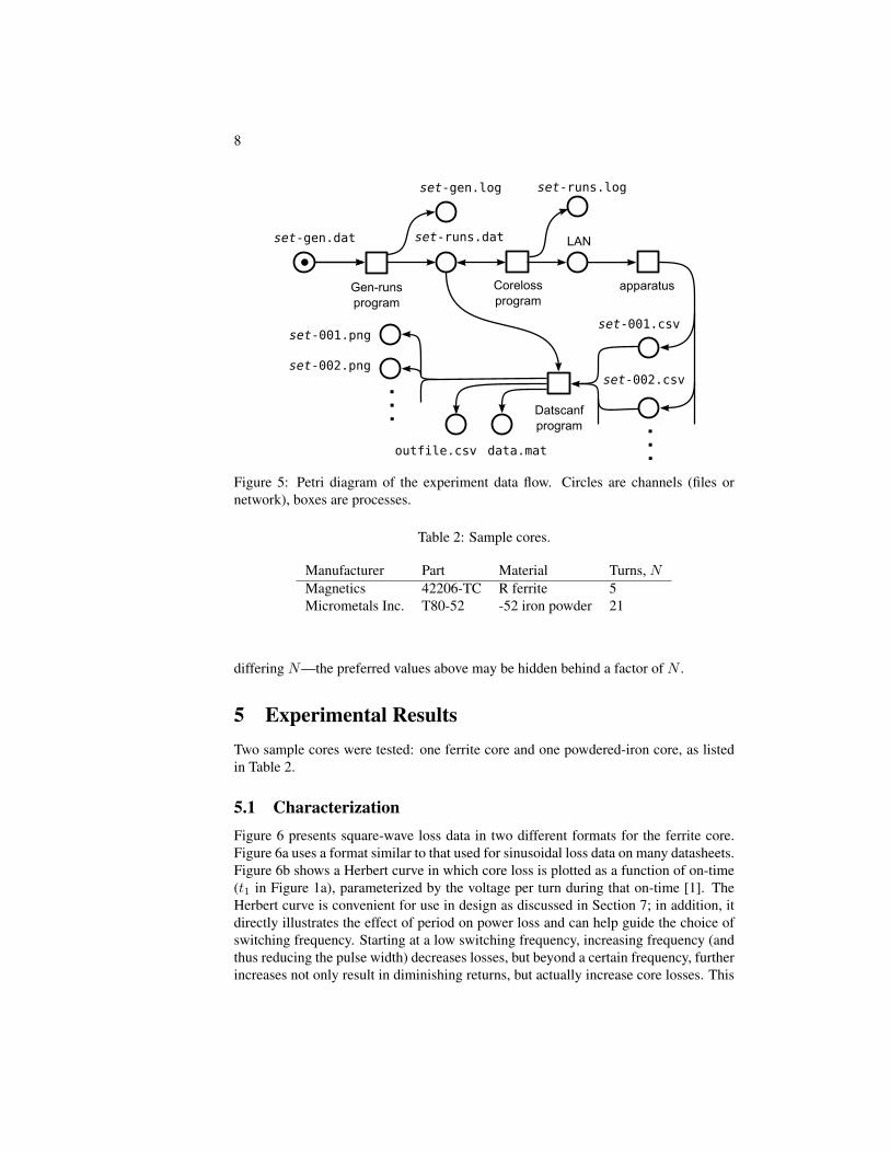
8

Gen-runs

program

Coreloss

program

apparatus

LANset-gen.dat

set-gen.log

set-runs.dat

set-001.csv

set-002.csv

Datscanf

program

set-001.png

set-002.png

set-runs.log

...

...data.matoutfile.csv

Figure 5: Petri diagram of the experiment data flow. Circles are channels (files ornetwork), boxes are processes.

Table 2: Sample cores.

Manufacturer Part Material Turns, NMagnetics 42206-TC R ferrite 5Micrometals Inc. T80-52 -52 iron powder 21

differing N—the preferred values above may be hidden behind a factor of N .

5 Experimental ResultsTwo sample cores were tested: one ferrite core and one powdered-iron core, as listedin Table 2.

5.1 CharacterizationFigure 6 presents square-wave loss data in two different formats for the ferrite core.Figure 6a uses a format similar to that used for sinusoidal loss data on many datasheets.Figure 6b shows a Herbert curve in which core loss is plotted as a function of on-time(t1 in Figure 1a), parameterized by the voltage per turn during that on-time [1]. TheHerbert curve is convenient for use in design as discussed in Section 7; in addition, itdirectly illustrates the effect of period on power loss and can help guide the choice ofswitching frequency. Starting at a low switching frequency, increasing frequency (andthus reducing the pulse width) decreases losses, but beyond a certain frequency, furtherincreases not only result in diminishing returns, but actually increase core losses. This

rev 9a 9

point corresponds to pulse widths of 1.5 to 3 µs for the ferrite material tested, andthus periods of 3 to 6 µs, and square-wave frequencies of 167 to 333 kHz. This isgenerally consistent with the behavior seen in plots of “performance factor” B · f forfixed power loss provided by some manufacturers [28, 29, 30]. However, the frequencybeyond which performance degrades is lower in our data than in plots of performancefactor for the same material (about 600 kHz [28]), presumably because of the harmonicenergy content of the square-wave excitation.

Square-wave loss data for the powdered-iron core is shown in the same two formatsin Figure 7, and shows similar trends though the values are different.

5.2 Verification

Additional data was collected to assess the accuracy of the method described in Sec-tion 3 for predicting loss for other waveforms using only data from square-wave mea-surements. The first category of these tests is experiments using asymmetric wave-forms as shown in Figure 1b (upper right). The results of these experiments are plottedin Figure 8. Each curve is for fixed width and amplitude of the first pulse (fixed V1

and t1 as defined in Figure 1a) with the width of the second pulse (t2) varying. Theamplitude of the second pulse was adjusted for zero average voltage. The widths andamplitudes were all chosen to match data in the original characterization data set suchthat no interpolation was needed to predict loss, and the energy loss per cycle could bepredicted from two points in the characterization data: the energy loss per cycle for asquare wave of amplitude V1 and half-period t1 (Esqr(V1, t1)) and the energy loss percycle for a square wave of amplitude V2 and half-period t2, as

Ec =12

(Esqr(V1, t1) + Esqr(V2, t2)) (2)

The measured asymmetric waveform loss is compared to loss predicted from (2) in Fig-ure 8, showing excellent matching over a wide range of asymmetry ratios (t1/T ) andamplitudes, for both the ferrite core and the powdered iron core. This confirms that thecomposite waveform hypothesis is a good approximation for asymmetric waveforms.

Test results for waveforms with a zero-voltage time t0 between pulses are shown inFigures 9 and 10. In each test, the positive and negative voltage pulses have constantamplitude and duration (as listed in the figure legend), but the zero-voltage time be-tween pulses, t0, is varied. In Figures 9a and 10a, the waveform is always symmetricand the overall period is expanded as t0 is increased (marked “Symmetric, D < 1”in Figure 1b). In Figures 9b and 10b, the period remains constant but the waveformis skewed with one of the two zero-voltage periods shrinking as the other expands(marked “Shifted, D < 1” in Figure 1b).

Based on the composite waveform hypothesis (see Section 3), we would expectFigures 9a and 10a to show constant energy loss per cycle as the zero-voltage time, andthus the period, increases, with no loss occurring during the zero-voltage time. The datain Figure 9a, for the ferrite core, show significant variations as t0 increases, as much asabout 40%, in some cases increasing and in others decreasing. The data in Figure 10a,for the powdered-iron core, show much less variation, matching the expectation from

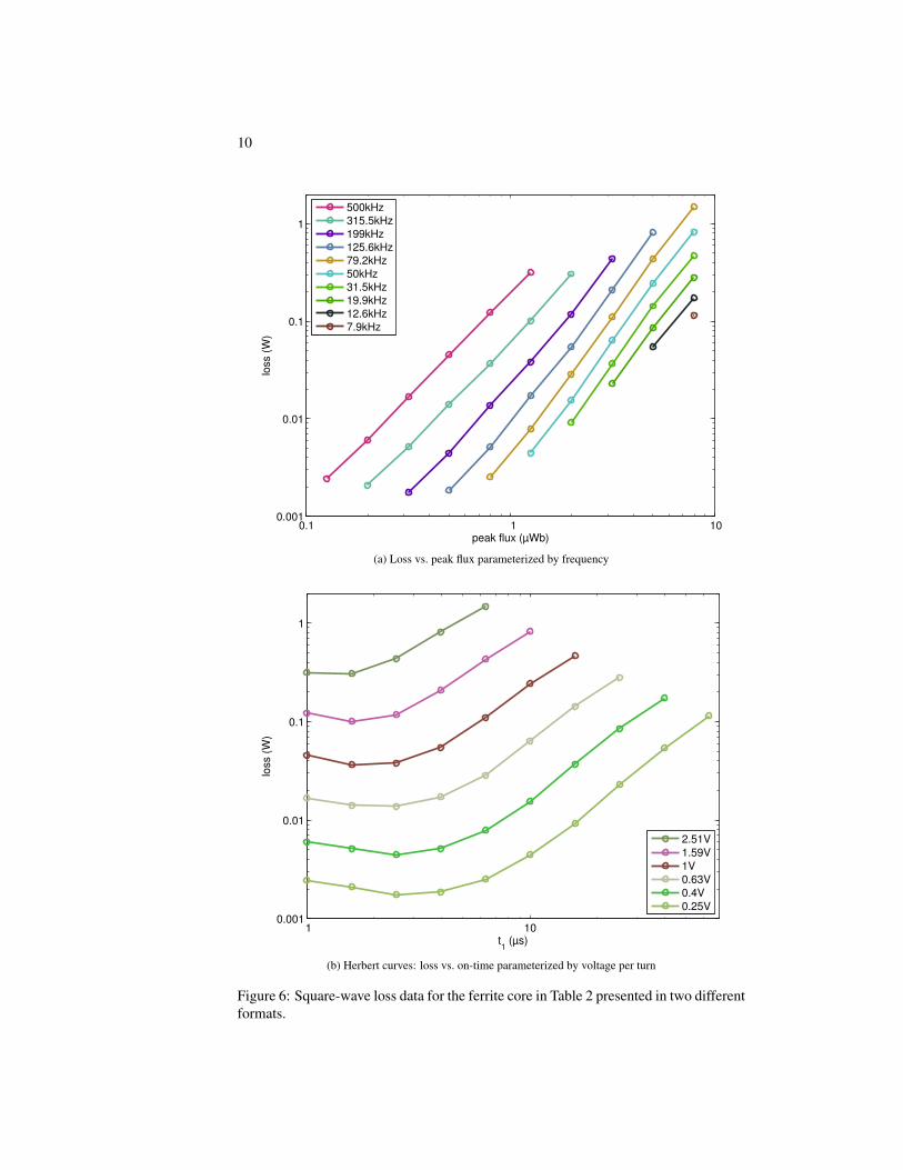
10

0.1 1 100.001

0.01

0.1

1

peak flux (µWb)

loss (

W)

500kHz

315.5kHz

199kHz

125.6kHz

79.2kHz

50kHz

31.5kHz

19.9kHz

12.6kHz

7.9kHz

(a) Loss vs. peak flux parameterized by frequency

1 100.001

0.01

0.1

1

t1 (µs)

loss (

W)

2.51V

1.59V

1V

0.63V

0.4V

0.25V

(b) Herbert curves: loss vs. on-time parameterized by voltage per turn

Figure 6: Square-wave loss data for the ferrite core in Table 2 presented in two differentformats.

rev 9a 11

0.1 1 10

0.001

0.01

0.1

1

peak flux (µWb)

loss (

W)

500kHz

315.5kHz

199kHz

125.6kHz

79.2kHz

50kHz

31.5kHz

19.9kHz

12.6kHz

(a) Loss vs. peak flux parameterized by frequency

1 10

0.001

0.01

0.1

1

t1 (µs)

loss (

W)

0.5V

0.32V

0.2V

0.13V

0.08V

0.05V

(b) Herbert curves: loss vs. on-time parameterized by voltage per turn

Figure 7: Square-wave loss data for the powdered-iron core in Table 2 presented in twodifferent formats.

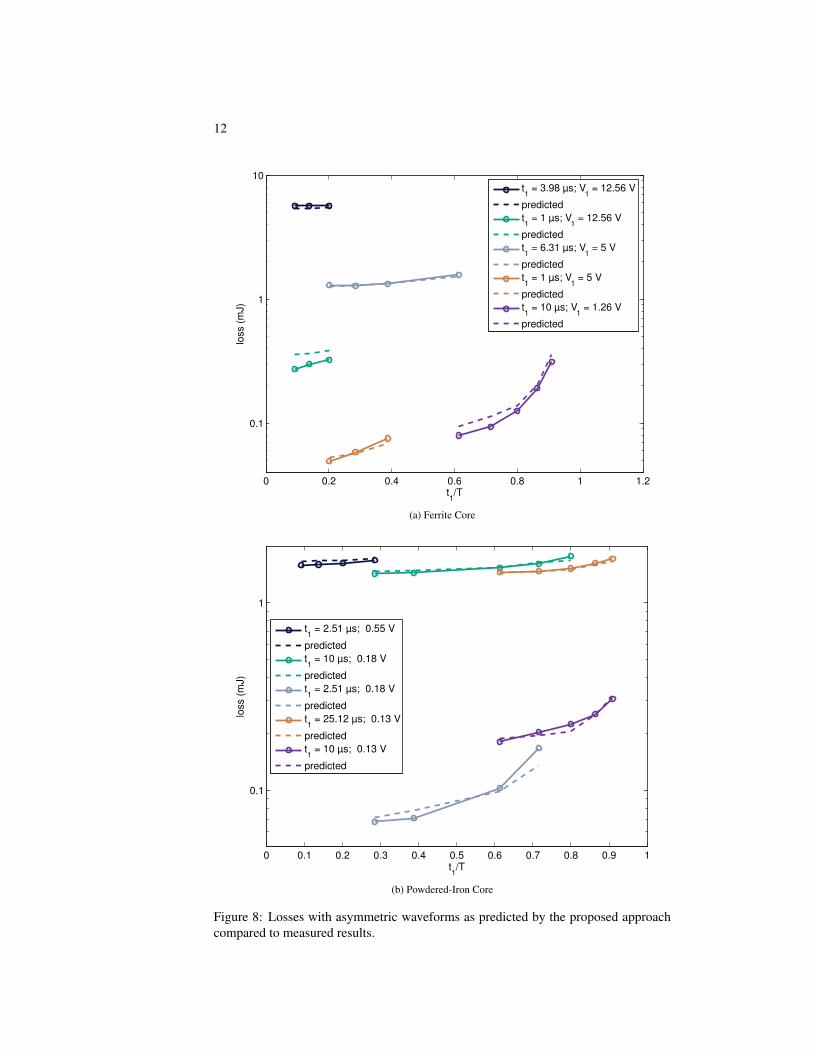
12

0 0.2 0.4 0.6 0.8 1 1.2

0.1

1

10

t1/T

loss (

mJ)

t1 = 3.98 µs; V

1 = 12.56 V

predicted

t1 = 1 µs; V

1 = 12.56 V

predicted

t1 = 6.31 µs; V

1 = 5 V

predicted

t1 = 1 µs; V

1 = 5 V

predicted

t1 = 10 µs; V

1 = 1.26 V

predicted

(a) Ferrite Core

0 0.1 0.2 0.3 0.4 0.5 0.6 0.7 0.8 0.9 1

0.1

1

t1/T

loss (

mJ)

t1 = 2.51 µs; 0.55 V

predicted

t1 = 10 µs; 0.18 V

predicted

t1 = 2.51 µs; 0.18 V

predicted

t1 = 25.12 µs; 0.13 V

predicted

t1 = 10 µs; 0.13 V

predicted

(b) Powdered-Iron Core

Figure 8: Losses with asymmetric waveforms as predicted by the proposed approachcompared to measured results.

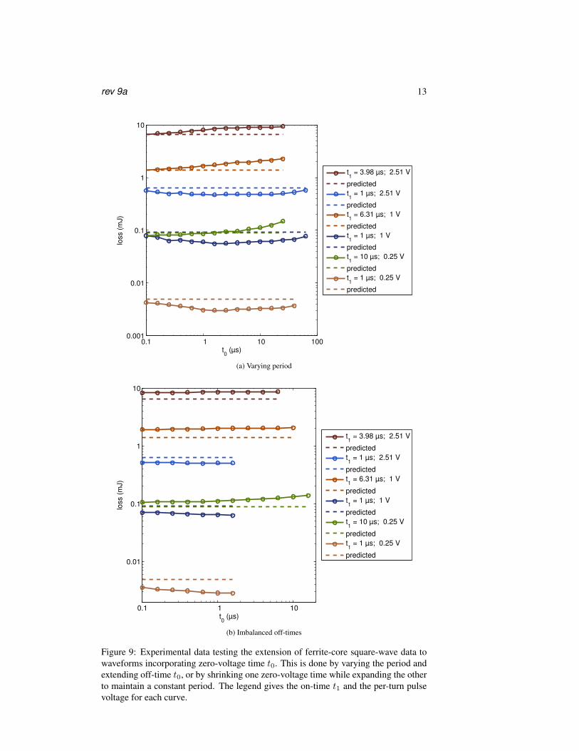
rev 9a 13

0.1 1 10 1000.001

0.01

0.1

1

10

t0 (µs)

loss (

mJ)

t1 = 3.98 µs; 2.51 V

predicted

t1 = 1 µs; 2.51 V

predicted

t1 = 6.31 µs; 1 V

predicted

t1 = 1 µs; 1 V

predicted

t1 = 10 µs; 0.25 V

predicted

t1 = 1 µs; 0.25 V

predicted

(a) Varying period

0.1 1 10

0.01

0.1

1

10

t0 (µs)

loss (

mJ)

t1 = 3.98 µs; 2.51 V

predicted

t1 = 1 µs; 2.51 V

predicted

t1 = 6.31 µs; 1 V

predicted

t1 = 1 µs; 1 V

predicted

t1 = 10 µs; 0.25 V

predicted

t1 = 1 µs; 0.25 V

predicted

(b) Imbalanced off-times

Figure 9: Experimental data testing the extension of ferrite-core square-wave data towaveforms incorporating zero-voltage time t0. This is done by varying the period andextending off-time t0, or by shrinking one zero-voltage time while expanding the otherto maintain a constant period. The legend gives the on-time t1 and the per-turn pulsevoltage for each curve.

14

1 10

0.01

0.1

1

10

100

t0 (µs)

loss (

mJ)

t1 = 25.12 µs; 0.5 V

predicted

t1 = 10 µs; 0.5 V

predicted

t1 = 2.51 µs; 0.5 V

predicted

t1 = 25.12 µs; 0.13 V

predicted

t1 = 10 µs; 0.13 V

predicted

t1 = 2.51 µs; 0.13 V

predicted

t1 = 25.12 µs; 0.05 V

predicted

t1 = 10 µs; 0.05 V

predicted

t1 = 2.51 µs; 0.05 V

predicted

(a) Varying period

1 10

0.01

0.1

1

10

100

t0 (µs)

loss (

mJ)

t1 = 25.12 µs; 0.5 V

predicted

t1 = 10 µs; 0.5 V

predicted

t1 = 2.51 µs; 0.5 V

predicted

t1 = 25.12 µs; 0.13 V

predicted

t1 = 10 µs; 0.13 V

predicted

t1 = 2.51 µs; 0.13 V

predicted

t1 = 25.12 µs; 0.05 V

predicted

t1 = 10 µs; 0.05 V

predicted

t1 = 2.51 µs; 0.05 V

predicted

(b) Imbalanced off-times

Figure 10: Experimental data testing the extension of powdered-iron-core square-wavedata to waveforms incorporating zero-voltage time t0. This is done by varying the pe-riod and extending on-time t1, or by shrinking one zero-voltage time while expandingthe other to maintain a constant period.

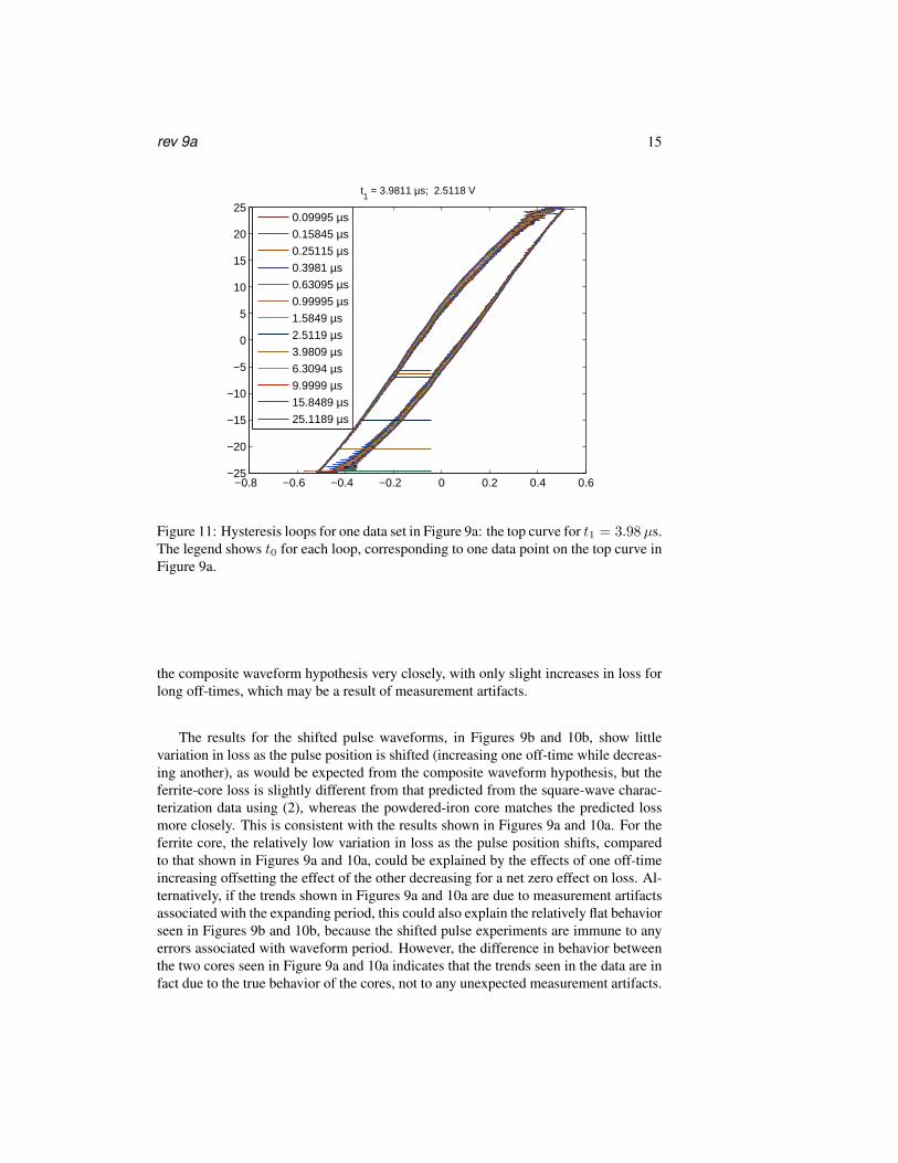
rev 9a 15

−0.8 −0.6 −0.4 −0.2 0 0.2 0.4 0.6−25

−20

−15

−10

−5

0

5

10

15

20

25

t1 = 3.9811 µs; 2.5118 V

0.09995 µs

0.15845 µs

0.25115 µs

0.3981 µs

0.63095 µs

0.99995 µs

1.5849 µs

2.5119 µs

3.9809 µs

6.3094 µs

9.9999 µs

15.8489 µs

25.1189 µs

Figure 11: Hysteresis loops for one data set in Figure 9a: the top curve for t1 = 3.98 µs.The legend shows t0 for each loop, corresponding to one data point on the top curve inFigure 9a.

the composite waveform hypothesis very closely, with only slight increases in loss forlong off-times, which may be a result of measurement artifacts.

The results for the shifted pulse waveforms, in Figures 9b and 10b, show littlevariation in loss as the pulse position is shifted (increasing one off-time while decreas-ing another), as would be expected from the composite waveform hypothesis, but theferrite-core loss is slightly different from that predicted from the square-wave charac-terization data using (2), whereas the powdered-iron core matches the predicted lossmore closely. This is consistent with the results shown in Figures 9a and 10a. For theferrite core, the relatively low variation in loss as the pulse position shifts, comparedto that shown in Figures 9a and 10a, could be explained by the effects of one off-timeincreasing offsetting the effect of the other decreasing for a net zero effect on loss. Al-ternatively, if the trends shown in Figures 9a and 10a are due to measurement artifactsassociated with the expanding period, this could also explain the relatively flat behaviorseen in Figures 9b and 10b, because the shifted pulse experiments are immune to anyerrors associated with waveform period. However, the difference in behavior betweenthe two cores seen in Figure 9a and 10a indicates that the trends seen in the data are infact due to the true behavior of the cores, not to any unexpected measurement artifacts.

16

−0.4 −0.3 −0.2 −0.1 0 0.1 0.2 0.3 0.4−20

−15

−10

−5

0

5

10

15

20

t1 = 6.3096 µs; 1 V

0.0999 µs

0.1584 µs

0.2514 µs

0.3979 µs

0.6309 µs

0.9999 µs

1.5849 µs

2.5119 µs

3.9809 µs

6.3094 µs

9.9999 µs

15.8489 µs

25.1189 µs

Figure 12: Hysteresis loops for one data set in Figure 9a: the second curve from thetop, for t1 = 6.31 µs. The legend shows t0 for each loop, corresponding to one datapoint on the second curve in Figure 9a.

6 Hysteresis Loops

To further explore the phenomena causing variations in loss when the zero-voltage timebetween pulses, t0, is varied, hysteresis loops for each point in several of the curves inFigure 9a are plotted in Figures 11, 12, and 13.

The scale and number of curves on these figures, together with ringing on the wave-forms, makes it difficult to see a dramatic trend, particularly on the relatively narrowloops of Figure 12 and Figure 13. However, a zoomed in view of Figure 11, shown inFigure 14, provides some insight. We see that the rise to the point of maximum currentand flux linkage is nearly identical on each curve, with the exception of ringing thathas little effect on the area of the loop. However, the decreases diverge: those with theshortest zero-voltage time t0 fall more directly, while those with longer zero-voltagetime curve further to the left. This part of the curve immediately follows the pauseat zero voltage (which is at the top right of the plot), and thus it makes sense that itsshape is the most affected by the pause. An oversimplified description would be thatthe flux gets “stuck” near the the maximum value if it has had time to “soak” and get

rev 9a 17

−0.2 −0.15 −0.1 −0.05 0 0.05 0.1 0.15−8

−6

−4

−2

0

2

4

6

8

t1 = 10 µs; 0.2512 V

0.1 µs

0.1585 µs

0.251 µs

0.398 µs

0.631 µs

1 µs

1.585 µs

2.512 µs

3.981 µs

6.3095 µs

10 µs

15.849 µs

25.119 µs

Figure 13: Hysteresis loops for one data set in Figure 9a: the fourth curve from the top,for t1 = 10 µs. The legend shows t0 for each loop, corresponding to one data point onthe fourth curve in Figure 9a.

accustomed to that flux value, whereas the flux can more easily transition away fromthe maximum if the excitation is decreased immediately.

7 Design TechniquesThe loss data derived from square-wave measurements can be provided to a magneticsdesigner in various forms, including tabulated data or curve-fit functions for use insoftware, and various types of graphical presentation. The loss data can be presentedas loss per unit volume, or as total loss for a specific core, to simplify calculationsfor the designer. Here we discuss working from graphical data in the “Herbert curve”format of Figure 6b. These curves are parameterized by voltage per turn applied to awinding. It’s also possible to provide curves like this for a specific component with agiven number of turns, parameterized by voltage.

In general, for waveforms as shown in Figure 1a, based on (2), one can calculateloss from a Herbert plot as

P =1T

(Psqr(V1/N, t1) · t1 + Psqr(V2/N, t2) · t2) (3)

In the case of symmetric waveforms, Psqr(V1/N, t1) = Psqr(V2/N, t2), and the losscalculation reduces to

P =2t1T

Psqr(V1/N, t1). (4)

18

−0.1 0 0.1 0.2 0.3 0.4 0.5

5

10

15

20

25

t1 = 3.9811 µs; 2.5118 V

0.09995 µs

0.15845 µs

0.25115 µs

0.3981 µs

0.63095 µs

0.99995 µs

1.5849 µs

2.5119 µs

3.9809 µs

6.3094 µs

9.9999 µs

15.8489 µs

25.1189 µs

Figure 14: A zoomed-in view of the hysteresis loops in Figure 11. The legend showst0 for each loop, corresponding to one data point on the top curve in Figure 9a.

Consider, for example, a component operating at 50 kHz with a symmetric wave-form with a duty cycle of 63%, 12 turns, and a pulse amplitude of 4.8 V. The period is20 µs, and the positive and negative pulse widths are t1 = t2 = 0.63 · 10 µs = 6.3 µs.To find the correct curve to examine in Figure 6b, we find the voltage per turn whichis 4.8/12 = 0.4 V. As shown in Figure 15, we can read off the power loss for this pulsewidth and voltage per turn as Psqr = 7.9 mW. According to (4) we scale this result bythe ratio 2t1/T = 12.6 µs/20 µs, to get a predicted power loss of 7.9 · 0.63 = 5 mW.

An interesting design space to explore is to maintain constant frequency and aver-age voltage, but to vary the pulse width and period. The relevant data is along a curveof constant volt-seconds on the Herbert plot—the dashed line in Figure 16. To getpower loss from these points, assuming constant frequency of 50 kHz, we then scalethese points down by the ratio 2 · t1/20 µs to get the solid line in Figure 16. This riseof this curve to the left illustrated the disadvantage of using shorter duty cycles for agiven average voltage or volt-second requirement.

As an asymmetric example, consider the same 12-turn winding, with a 12 V, 10 µspulse applied in one direction, and a 30 V, 4 µs pulse applied in the other direction,with a 20 µs overall period (50 kHz) as before (the waveform includes a total of 6 µsof zero-voltage time). Psqr(V1/N, t1) and Psqr(V2/N, t2) are read off Figure 15 as244 mW and 818 mW. The overall power loss can then be found from (3) as

P = 50 kHz (244 mW · 10 µs + 818 mW · 4 µs) = 286 mW. (5)

rev 9a 19

1 100.001

0.01

0.1

1

t1 (µs)

loss (

W)

2.51V

1.59V

1V

0.63V

0.4V

0.25V

Figure 15: Reading data from a Herbert plot for the examples discussed in the text.The lower red point marked with +× is for the first, symmetric example. The upper bluecircles are for the second, asymmetric example.

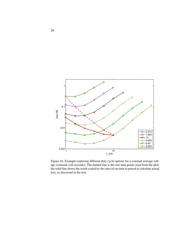
20

1 100.001

0.01

0.1

1

t1 (µs)

loss (

W)

2.51V

1.59V

1V

0.63V

0.4V

0.25V

Figure 16: Example exploring different duty cycle options for a constant average volt-age (constant volt-seconds). The dashed line is the raw data points used from the plot;the solid line shows the result scaled by the ratio of on-time to period to calculate actualloss, as discussed in the text.

rev 9a 21

8 DiscussionThe results in Figures 8 and 8b show that the composite waveform hypothesis holdswell for asymmetric waveforms, and the method provides excellent accuracy. Figure 10shows that, for the powdered-iron core tested, it also holds very well for waveformswith zero-voltage periods, although zero voltage times can cause significant deviationin the ferrite core tested. This variation is not predicted by the composite-waveformhypothesis; nor is it predicted by any of the methods discussed in Section 2. Additionalwork to better characterize and model this behavior could lead to more accurate losspredictions. However, even with this error, the approach described here is expected tobe more accurate than other methods which are subject to the same error, and addition-ally entail error due to using sinusoidal data to predict square-wave loss.

In addition to being more accurate than other methods, the new approach is alsoeasier to use than methods like the iGSE. Thus, we believe that it would be beneficialfor core manufacturers to characterize square-wave loss and provide that data graphi-cally, electronically or both, either on a per-unit-volume basis or on a per-core basis.

As presented here, the method is only applicable to waveforms with one positivevoltage pulse and one negative pulse. However, it could also be easily applied to wave-forms with minor loops by separating the minor loops following the approach in [7], aslong as each constituent loop comprises only one positive pulse and one negative pulse.Adapting the method to waveforms with a series of voltage pulses of the same polar-ity but differing amplitudes is less straightforward. The corresponding analysis in theiGSE (eq. (13) in [7]) includes a factor that depends on the total flux excursion as wellas the flux change for a given pulse, and it may be necessary to introduce similar factorsto accurately model losses in such cases using square-wave loss data. However, mostpower electronics applications use waveforms with only one positive voltage pulse andone negative pulse, such that that the analysis here applies directly.

22

9 Using the DataThe data generated by this works includes characterization data for two cores and ver-ification data for the same two cores. Complete data for both is archived at the website http://engineering.dartmouth.edu/inductor/coredata in filesferrite-data.zip and powdered iron-data.zip. However, a user calcu-lating loss for a particular waveform does not need these large (> 20MB) files, butrather needs only the characterization data. This data is available in a smaller data col-lection, characterization-data.zip, on the same page. This archive containsthe data plotted in Figures 6 and 7 in multiple formats, as well as the plots themselvesas Portable Network Graphics (PNG) images. The data include, for each square wavetested,

• Frequency (Hz).

• Peak flux linkage (Vs).

• Volts/turn.

• Average loss (W).

• Loss per cycle (J).

The formats are:

• Microsoft Excel (.xls) format, with columns corresponding to each of the datalisted above, and headings labeling each.

• Comma-separated value (.csv) format, with columns corresponding to each ofthe data listed above, and no text.

• Plain text (.dat) file, with columns corresponding to each of the data listedabove, and a header row briefly identifying each column.

• Matlab .mat format, which, when loaded into the Matlab environment, providesthe variables f, dphi, Vturn, Pavg, and Ecycle, corresponding to the datalisted above.

These formats are explained in greater detail in the appendix.Many users may wish to simply read values off of the graphs in Figures 6 and 7 but

these files make the data available in multiple formats for use by computer software, orfor analyzing, curve-fitting, or plotting the data.

10 ConclusionThe proposed measurement and loss calculation approach allows generalizing square-wave core-loss data to predict core loss with any common rectangular voltage wave-form. An automated measurement system has been used to collect the required square-wave core characterization data for ferrite and powdered-iron cores, and to collect addi-tional data to assess the accuracy of the method for other voltage waveforms. Measure-ments show good correlation, but also exhibit behavior not yet explained by published

rev 9a 23

models, which may lead to new insights and more accurate models. Despite the minordiscrepancies, the loss prediction method yields higher accuracy, and is easier to use,than other methods for non-sinusoidal waveforms.

24

A Data Files and FieldsThis appendix summarizes the various field names in the data files, along with theirmeanings. Table 3 gives a summary of all the files. In these files, we use designationsto identify the four waveform types shown in Figure 1b. They are listed in Table 4.

A.1 Oscilloscope DataThe first two lines of the oscilloscope CSV files are heading. The first is the fieldidentifier, the second, the units of measure. All the data are floating point numbers.The SYNC and OUT fields are the input to the waveform decoder and are only used fordebugging.

x-axis Time, in seconds.

SYNC The sync signal from the arbitrary waveform generator (volts).

OUT The output signal from the arbitrary waveform generator (volts).

V The sense winding voltage, Vs, (volts).

Field Descriptionset-gen.dat The Gen-runs input data file, instructions for making a set of

runs.set-runs.dat The output from Gen-runs and the input to the Coreloss pro-

gram.set-gen.log A log file from Gen-runs echoing the parameters and telling

which runs were skipped and why.set-log.dat A diagnostic file created by the Coreloss program.set-log.csv A diagnostic file created by the Coreloss program. It has the

same informations as the .dat file, above, but in the CSV for-mat.

set-run.csv The output from the oscilloscope for a single run.set-run.txt A configuration log from the oscilloscope for a single run.set-run.png An image of a plot of the oscilloscope data for a single run,

along with a plot of power and energy versus time.output.dat Contains the per-cycle loss data, as well as the original data.output.csv Contains the per-cycle loss data, as well as the original data. It

has the same informations as the .dat file, above, but in theCSV format.

data.mat Contains the per-cycle loss data, as well as the original data.It has the same informations as the .dat file, above, but asMatlab source code.

Table 3: File naming conventions for parameter and data files.

rev 9a 25

Designation D t1 = t2 Symmetric Commentsquare = 1 yes yesskew < 1 yes no “shifted”expand < 1 yes yes varying Tassym = 1 no no

Table 4: Waveform type designations

I The current (amperes).

A.2 Test Input DataThe test input file read by the Coreloss program. Each record is a white-space-delimitedlist of the parameters for one run. An experimental run has these parameters:

runId The run identifier. This should chosen to be be globally unique. The Gen-runsprogram uses the set ID, followed by a zero-padded integer, the run ID.

sample The core sample identifier.

N The number of turns on the core.

period The period, T , of the drive voltage, in seconds. (Floating point.)

t1 The pulse width of the first pulse. (Floating point.)

pinch The pinch, P , it the time between pulse 1 and pulse 2, t0, expressed as a fractionof the off time for a symmetric waveform:

P = 1− 2t0T − t1 − t2

0 ≤ P ≤ 1 for D < 1. P = 1 for expand waveforms, and is undefined forD = 1 (indicated in the file by -1). (Floating point.)

D=1 A Boolean value, true (1) if D = 1 and 0 otherwise. This may seem redundant,but it is needed for clarity and safety because of the floating point time parame-ters.1

Vps It is the voltage requested from the power supply.

delay A delay between runs to allow for cooling. (Seconds.)

VRange Full scale voltage range setting for the oscilloscope.

IRange Full scale current range setting for the oscilloscope.

The following fields are used by the data reduction programs to group data by families:

1The name D=1 was chosen for brevity and clarity. I hope the embedded math symbol is not confusing.

26

TSet Zero if it is not a square wave. Otherwise, records with the same value havethe same period.

VSet Zero if it is not a square wave. Otherwise, records with the same value havethe same Vps.

expandSet Zero if it is not an expand waveform. Otherwise, records with the samevalue have the same pulse shape. (Varying t0.)

skewSet Zero if it is not a skew waveform. Otherwise, records with the same valuehave the same pulse shape. (Varying P .)

assymSet Zero if it is not a assym waveform. Otherwise, records with the same valuehave the same pulse shape for the t1 pulse.

A.3 Run Data GeneratorThe input file for Gen-runs is a white-space-delimited dictionary. The fields are:

comment This is a one-line comment that is printed at the top of the run data file.

setId The set ID is used to name the run data file and is prepended to each run ID.By convention, this is the same as the set identifier used in the source data filenames.

sample The identifier for the core sample.

N The number of turns.

types A list of run types to be generated. They can be any of square, expand,skew, assym.

t1min Minimum pulse width for square wave runs.

t1max Maximum pulse width for square wave runs.

VpsMin Minimum power supply voltage.

VpsMax Maximum power supply voltage.

grid Spacing of the geometric series, in decilog. For five values per decade, use 2.

satLimit Saturation limit in power supply volt-seconds per turn.

delay The delay time for cooling between runs, in seconds.

expandSamples A white-space-delimited, paired list of Vps/N and t1 for the pulsesused in expand and skew runs. These values will be “rounded” to the decilogpreferred values (Section 4.2).

t0min The minimum off-time between pulses, t0, to be used for expand and skewruns.

rev 9a 27

t0max For expand and skew runs, the maximum off-time. expand waveformsare symmetric, with the period T = 2(t1 + t0). The off time, t0, increasesgeometrically, stopping when it exceeds t0max.

TFactor For skew runs, the ratio of the period, T , to the pulse width, used to deter-mine T , i.e., the period is TFactor * t1. The series starts with t0 = t0 min,and increases t0 geometrically until the pulses are approximately symmetric.

# For comments; both the key (#) and the value are ignored by the program.

B General File FormatsThere a few general types of file format used in the project:

Comma separated value (CSV). This is a standard tabular format, where columnsare separated by commas. Files have the .csv extension. It was chosen be-cause it was the only ASCII text output file format available from the Tektronixoscilloscope. The first line or two of all the CSV files is a header.

Key-value dictionary. This is a particularly nice, human and machine readable formatfor configuration files. Each line has zero or more white-space-delimited key-value pairs. The key is a unique parameter name; the value is the value it isassigned. The layout and order of the pairs is unimportant. If a value is enclosedin quotation marks or braces, it may be empty or contain embedded white space.

Log. Log files are text files and usually have the extension .log. They give diagnosticinformation and are intended for human readers, and are generally not easilyparsed by a computer.

White space delimited table. These are ASCII text table files that separate columnswith white space—spans of one or more space or tab characters. They are easilyread by a human if printed with a monospaced font, like Courier. Cells that areempty, or contain white space, must be enclosed in quotation marks or braces.Blank lines and lines beginning with # are ignored. The latter are often used forheadings.

Portable network graphic (PNG). These are raster graphics files, used for the dataplots.

Matlab MathWorks MATLAB source code file, which have the extension .mat.

28

AcknowledgementsThanks to the Power Sources Manufacturers’ Association and the National Institute forStandards and Technology (NIST) for support of this work.

References[1] Edward Herbert. User-friendly data for magnetic core loss calculations. August

2008. http://fmtt.com/Coreloss2009.pdf.

[2] M. Albach, T. Durbaum, and A. Brockmeyer. Calculating core losses in trans-formers for arbitrary magnetizing currents a comparison of different approaches.In 27th Annual IEEE Power Electronics Specialists Conference, volume 2, pages1463–8, June 1996.

[3] J. Reinert, A. Brockmeyer, and R.W. De Doncker. Calculation of losses in ferro-and ferrimagnetic materials based on the modified Steinmetz equation. In Pro-ceedings of 34th Annual Meeting of the IEEE Industry Applications Society, pages2087–92 vol.3, 1999.

[4] A. Brockmeyer. Dimensionierungswekzeug fur magnetische Bauelemente inStromrichteranwendungen. PhD thesis, Aachen University of Technology, 1997.

[5] Jinjun Liu, T. G. Wilson, Jr., R. C. Wong, R. Wunderlich, and F. C. Lee. A methodfor inductor core loss estimation in power factor correction applications. In Pro-ceedings of APEC 2002—Applied Power Electronics Conference and Exposition,page 439, 2002.

[6] Jieli Li, T. Abdallah, and C. R. Sullivan. Improved calculation of core loss withnonsinusoidal waveforms. In IEEE Industry Applications Society Annual Meet-ing, pages 2203–2210, 2001.

[7] K. Venkatachalam, C. R. Sullivan, T. Abdallah, and H. Tacca. Accurate pre-diction of ferrite core loss with nonsinusoidal waveforms using only Steinmetzparameters. In IEEE Workshop on Computers in Power Electronics, 2002.

[8] A.P. Van den Bossche, D.M. Van de Sype, and V.C. Valchev. Ferrite loss mea-surement and models in half bridge and full bridge waveforms. In IEEE PowerElectronics Specialists Conference, pages 1535–1539, June 2005.

[9] Alex van den Bossche and Vencislav Valchev. Inductors and Transformers forPower Electronics. Taylor and Francis Group, 2005.

[10] S. Mulder. Power ferrite loss formulas for transformer design. Power Conversion& Intelligent Motion, 21(7):22–31, July 1995.

[11] E. C. Snelling. Soft Ferrites, Properties and Applications. Butterworths, secondedition, 1988.

rev 9a 29

[12] C. P. Steinmetz. On the law of hysteresis. AIEE Transactions, 9:3–64, 1892.Reprinted under the title “A Steinmetz contribution to the ac power revolution”,introduction by J. E. Brittain, in Proceedings of the IEEE 72(2) 1984, pp. 196–221.

[13] A. Brockmeyer. Experimental evaluation of the influence of dc-premagnetizationon the properties of power electronic ferrites. In APEC ’96. Eleventh AnnualApplied Power Electronics Conference, pages 454–60, 1996.

[14] A. Brockmeyer and J. Paulus-Neues. Frequency dependence of the ferrite-loss in-crease caused by premagnetization. In Twelfth Annual Applied Power ElectronicsConference and Exposition, pages 375–80, 1997.

[15] Wai Keung Mo, D.K.W. Cheng, and Y.S. Lee. Simple approximations of the dcflux influence on the core loss power electronic ferrites and their use in design ofmagnetic components. IEEE Transactions on Industrial Electronics, 44(6):788–99, 1997.

[16] G. Bertotti. General properties of power losses in soft ferromagnetic materials.IEEE Transactions on Magnetics, 24(1):621–630, 1988.

[17] G. Bertotti. Hysteresis in magnetism: for physicists, materials scientists, andengineers. Academic Press, 1998.

[18] K. H. Carpenter. Simple models for dynamic hysteresis which add frequency-dependent losses to static models. IEEE Transactions on Magnetics, 34(3):619–22, 1998.

[19] J.-T. Hsu and K. D. T. Ngo. A Hammerstein-based dynamic model for hysteresisphenomenon. IEEE Transactions on Power Electronics, 12(3):406–413, 1997.

[20] H. Saotome and Y. Sakaki. Iron loss analysis of Mn-Zn ferrite cores. IEEETransactions on Magnetics, 33(1):728–34, 1997.

[21] W. Roshen. Ferrite core loss for power magnetic components design. IEEETransactions on Magnetics, 27(6):4407–15, 1991.

[22] P. Tenant and J. J. Rousseau. Dynamic model of magnetic materials applied onsoft ferrites. IEEE Transactions on Power Electronics, 13(2):372–9, 1998.

[23] F. Fiorillo and A. Novikov. An improved approach to power losses in mag-netic laminations under nonsinusoidal induction waveform. IEEE Transactionson Magnetics, 26(5):2904–10, 1990.

[24] D. C. Jiles. Frequency dependence of hysteresis curves in ’non-conducting’ mag-netic materials. IEEE Transactions on Magnetics, 29(6):3490–2, 1993.

[25] Wei Shen, Fei (Fred) Wang, Dushan Boroyevich, and C. Wesley Tipton. Losscharacterization and calculation of nanocrystalline cores for high-frequency mag-netics applications. IEEE Transactions on Power Electronics, 23(1), 2008.

30

[26] Ray Ridley and Art Nace. Modeling ferrite core losses. Switching Power Maga-zine, 3(1):6–13, 2002.

[27] Christopher Oliver. A new core loss model. Switching Power Magazine, 3(2),2002.

[28] Ferrite material selection guide, 2000. Magnetics Division of Spang & Company,Bulletin No. FC-S1.

[29] Soft ferrites and accessories, data handbook, 2009. Ferroxcube, Eindhoven, TheNetherlands.

[30] Ferrites and accessories: SIFERRIT materials, 2006. EPCOS AG, Munich, Ger-many.

[31] K. H. Carpenter and S. Warren. A wide bandwidth, dynamic hysteresis model formagnetization in soft ferrites. IEEE Transactions on Magnetics, 28(5):2037–41,1992.

[32] I. D. Mayergoyz. Mathematical models of hysteresis. Springer-Verlag, 1991.

[33] Ping Han, G. R. Skutt, Ju Zhang, and F. C. Lee. Finite element method for ferritecore loss calculation. In Applied Power Electronics Conference and Exposition,volume 1, pages 348–353, 1995.

Testing Core Loss for Rectangular Waveforms,

Phase II Final Report

21 September 2011

Charles R. Sullivan John H. Harris

Thayer School of Engineering at Dartmouth charles.r.sullivan@dartmouth.edu

http://engineering.dartmouth.edu/inductor 8000 Cummings Hall

Hanover, NH 03755, USA

Sponsored by The Power Sources Manufacturers Association

email: power@psma.com http://www.psma.com/

P.O. Box 418 Mendham, NJ 07945-0418

Tel: (973) 543-9660 Fax: (973) 543-6207

Testing Core Loss

for Rectangular Waveforms,

Phase II Final Report

Charles R. Sullivan, John H.Harris

Thayer School of Engineering at Dartmouth

charles.r.sullivan@dartmouth.edu

http://engineering.dartmouth.edu/inductor

8000 Cummings Hall, Hanover, NH 03755, USA

21 September 2011

Summary

The Switching Power Converter Core Loss Project, Phase II is a follow-on to the Switching Power Converter Core Loss Pilot Project, conductedin 2009 [1]. In Phase II, we have accomplished these additional objectives:

• Gathered data on many more materials, particularly ferrites, andfurther validated the composite waveform hypothesis. More than4000 experimental runs were performed.

• We confirmed that core losses per cycle increase when the voltagewaveform includes off-time. This phenomenon was first noted inthe Phase I project. Additional testing established that it is a realphenomenon, and not an artifact of the testing procedure. We alsodeveloped an alternative waveform that does not exhibit this behav-ior.

• Measurements were performed with a drilled core having embeddingsense windings, looking for transient flux migration that might helpexplain off-time core loss.

• We developed a Steinmetz-like curve fit, and applied it to all the corecharacterization data. For the first time, a formula is available topredict loss accurately over a wide frequency range, avoiding glitchesbetween frequency ranges that occur with other models. Further-more, the model directly predicts loss with rectangular waveforms.It is available in different forms for different applications.

• We investigated the possibility of accidental residual magnetizationbiasing measurement results. We developed an automatic degauss-ing technique, and by comparing with previous results, we did notdiscover any evidence that the Phase I results were affected by suchspurious magnetization.

There are four appendices to this report. In Appendix A, we illustratethat core loss of non-sinusoidal waveforms cannot be accurately predictedby separately examining the Fourier components of the waveform. InAppendix B, we provide an example of the use of the composite waveformmodel in a design application. In Appendix C we provide additional dataplots. And in Appendix E we provide a a table with additional details ofthe Steinmetz-like loss modeling.

All of the data collected for this project accompany this report and areavailable for use by anyone. Full data from more than 4000 experimentalruns are archived. For information about using the data generated in theproject, see Using the PSMA Rectangular Waveform Core Loss Data [2].

ii

Contents

1 Introduction 1

2 The Basic Experiment 1

3 Broader Data Set 4

4 Drilled Core Experiments 4

4.1 Geometry . . . . . . . . . . . . . . . . . . . . . . . . . . . . . . . 44.2 Experimental Setup . . . . . . . . . . . . . . . . . . . . . . . . . 64.3 Observations . . . . . . . . . . . . . . . . . . . . . . . . . . . . . 7

5 Steinmetz Curve Fits 11

5.1 Model in Terms of Pulse Width and Voltage . . . . . . . . . . . . 14

6 Dead-Time Loss 14

6.1 Measurement Artifacts . . . . . . . . . . . . . . . . . . . . . . . . 146.2 Zero-Flux Off Time . . . . . . . . . . . . . . . . . . . . . . . . . . 166.3 An Improved “Predicted” Model . . . . . . . . . . . . . . . . . . 176.4 Conclusion . . . . . . . . . . . . . . . . . . . . . . . . . . . . . . 18

7 Degaussing 18

8 Using the Data 20

9 Future Work 20

9.1 Modeling . . . . . . . . . . . . . . . . . . . . . . . . . . . . . . . 219.2 Hardware . . . . . . . . . . . . . . . . . . . . . . . . . . . . . . . 219.3 Flux Spatial Dynamics . . . . . . . . . . . . . . . . . . . . . . . . 229.4 Design Implications . . . . . . . . . . . . . . . . . . . . . . . . . . 22

10 Conclusion 22

Appendices

A Steinmetz Harmonic Analysis 24

B Example Application 26

B.1 Conventional Parameters . . . . . . . . . . . . . . . . . . . . . . 26B.2 Pulse width and Voltage as Parameters . . . . . . . . . . . . . . 28

C Characterization Plots 29

C.1 Conventional Core Loss Plots . . . . . . . . . . . . . . . . . . . . 29C.2 Herbert Curves . . . . . . . . . . . . . . . . . . . . . . . . . . . . 30C.3 Hysteresis Plots . . . . . . . . . . . . . . . . . . . . . . . . . . . . 31

D Expand Plots 32

iii

E Extended Steinmetz Table 36

List of Tables

1 Cores tested in the project. . . . . . . . . . . . . . . . . . . . . . 52 Two-plane Steinmetz parameters . . . . . . . . . . . . . . . . . . 133 Published Steinmetz parameters . . . . . . . . . . . . . . . . . . 254 Example design parameters. . . . . . . . . . . . . . . . . . . . . . 265 Calculated square-wave loss. . . . . . . . . . . . . . . . . . . . . . 276 More two-plane Steinmetz parameters . . . . . . . . . . . . . . . 37

List of Figures

1 Full-bridge excitation circuit. . . . . . . . . . . . . . . . . . . . . 22 Block diagram of the experimental apparatus. . . . . . . . . . . 33 Excitation waveforms. . . . . . . . . . . . . . . . . . . . . . . . . 34 Toroidal core with added constriction. . . . . . . . . . . . . . . . 45 Drilled core and the subsection grid. . . . . . . . . . . . . . . . . 56 Flux distribution between subsections. . . . . . . . . . . . . . . . 77 Flux distribution, showing a transient disturbance. . . . . . . . . 88 Central annulus flux distribution. . . . . . . . . . . . . . . . . . . 89 Flux migration . . . . . . . . . . . . . . . . . . . . . . . . . . . . 910 Raw oscilloscope data plot . . . . . . . . . . . . . . . . . . . . . . 1011 Two-plane Steinmetz curve fit . . . . . . . . . . . . . . . . . . . . 1212 expand waveform core loss vs. off time . . . . . . . . . . . . . . . 1513 asym waveform core loss vs. asymmetry . . . . . . . . . . . . . . 1514 skew core loss vs. t0 . . . . . . . . . . . . . . . . . . . . . . . . . 1615 hippo waveform loss vs. off time. . . . . . . . . . . . . . . . . . . 1716 Example design voltage waveform . . . . . . . . . . . . . . . . . . 2717 Herbert plot for Ferroxcube 3C81 . . . . . . . . . . . . . . . . . . 3018 Hysteresis plot for Ferroxcube 3C81 . . . . . . . . . . . . . . . . 3119 expand core loss vs. off-time for Ceramic Magnetics MN60. . . . 3220 expand core loss vs. off-time for Ceramic Magnetics MN8CX. . . 3221 expand core loss vs. off-time for Ferroxcube 3C81. . . . . . . . . 3322 expand core loss vs. off-time for Ferroxcube 3C90. . . . . . . . . 3323 expand core loss vs. off-time for Ferroxcube 3F3. . . . . . . . . . 3324 expand core loss vs. off-time for Magnetics F. . . . . . . . . . . . 3425 expand core loss vs. off-time for Magnetics K. . . . . . . . . . . . 3426 expand core loss vs. off-time for Magnetics L. . . . . . . . . . . . 3427 expand core loss vs. off-time for Magnetics P. . . . . . . . . . . . 3528 expand core loss vs. off-time for Magnetics R. . . . . . . . . . . . 3529 expand core loss vs. off-time for Magnetics W. . . . . . . . . . . 35

iv

1 Introduction

In the design of magnetics for switching power applications, it is essential toaccurately estimate core loss, but current methods based on sinusoidal data aredifficult to use and inaccurate. Phase I of this project established the feasibilityand value of a new method proposed by Herbert [3], in which a simplified set ofsquare-wave measurements produces data that can be used to calculate loss forany alternating rectangular-voltage waveform.

The hypothesis to be tested was that, for alternating rectangular pulses anda given magnetic core material, the core loss energy per period depends only oncomponent pulse widths and peak voltages. We call this the composite waveformhypothesis (CWH).

In Phase I of the program, we established that this hypothesis, while notperfect, works well enough to be a significant improvement in both accuracy andease of use, compared with methods based on sinusoidal data. It is convenientto decompose rectangular waveforms into such pulses for analysis. Thus, it issufficient to test cores with square voltage waveforms, and then use the data topredict losses with generalized rectangular voltage waveforms.

Phase II of the project addresses these additional objectives:

1. To gather more square wave data to characterize additional core materialsand geometries, as well as validation data, to further test the CWH.

2. To investigate the dynamics of core flux distribution using embedded sensewindings.

3. To provide Steinmetz or similar curve-fitting parameters, for use in nu-merical design techniques.

4. To investigate the anomalous results discovered in Phase I involving pro-longed off-time waveforms.

5. To investigate the possibility of experimental error due to residual mag-netization in sample cores.

6. To demonstrate the use to this methodology in a design application.

7. To demonstrate the shortcomings of core loss estimates obtained by sum-ming sinusoidal Steinmetz estimates for rectangular waveform harmonics.

8. To improve data management and presentation to make the results moreaccessible to users.

In the sections that follow, we discuss the topics listed above in detail.

2 The Basic Experiment

In the basic experiment, a magnetic core is driven with a full bridge switchingcircuit (Figure 1). There is a second sense winding for measuring flux, to avoid

1

A

B D

C

DUT

i

+ vs

Figure 1: Full-bridge excitation circuit. The device under test (DUT) is amagnetic core.

measuring resistive loss in the drive winding. A blocking capacitor insures zeronet DC current. In most tests, the capacitor voltage is negligible, and is onlyneeded to cancel small volt-second mismatched due to timing errors. However,asymmetric waveforms are implemented by using significantly different on-timesfor positive and negative pulses. The capacitor voltage automatically adjusts toreduce the voltage of the longer pulse in order to have equal volt seconds betweenpositive and negative pulses. Our apparatus is capable of taking measurementsin a range of about 5 kHz to 500 kHz. The sample core is oil cooled, usuallykept at 80 C.

We take measurements with an Agilent Technologies DSO 7104A oscillo-scope. Current is measured with a Tektronix P 6021 AC current probe. Theswitching bridge is controlled by a programmable function generator with someadditional logic. This determines the frequency and pulse lengths. The bridgepower supply voltage determines the voltage amplitude. All three instrumentsare under the control of a computer, which orchestrates sets of experimentsand manages the resulting data (Figure 2). The oscilloscope sweep time is oneperiod. It averages the information from 512 triggers, and saves voltage andcurrent information at 1000 time-points per period.

We refer to one of these experiment as a run—think of a run as singlecaptured waveform. A run takes only a few seconds, but wound cores arenormally tested with a batch of runs, called a run set, in which frequency,amplitude, and pulse widths are varied from run to run. Run sets always includesquare wave runs, which characterize the coil under test. Data from more than4000 runs have been collected and accompany this report. Other wave forms(Figure 3) are also usually included to provide validation of the CWH, or forexploring other phenomena.

2

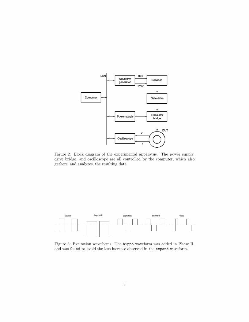
Figure 2: Block diagram of the experimental apparatus. The power supply,drive bridge, and oscilloscope are all controlled by the computer, which alsogathers, and analyzes, the resulting data.

Square Expanded SkewedAsymetric Hippo

Figure 3: Excitation waveforms. The hippo waveform was added in Phase II,and was found to avoid the loss increase observed in the expand waveform.

3

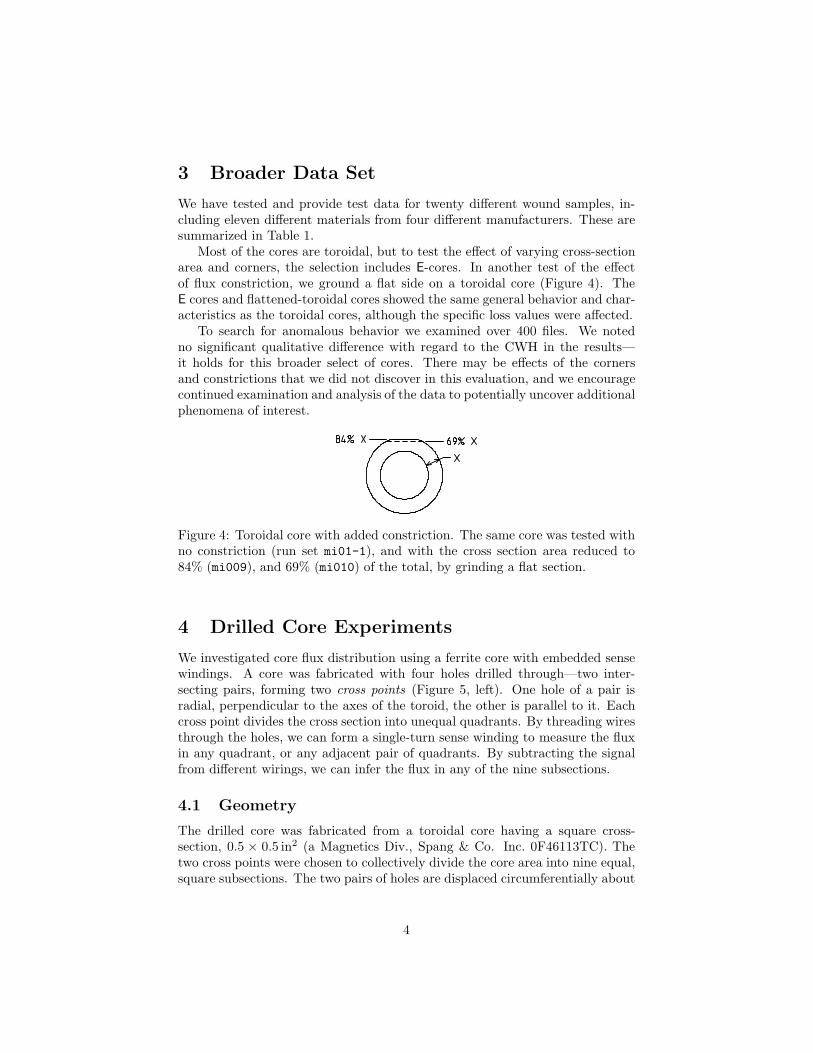
3 Broader Data Set

We have tested and provide test data for twenty different wound samples, in-cluding eleven different materials from four different manufacturers. These aresummarized in Table 1.

Most of the cores are toroidal, but to test the effect of varying cross-sectionarea and corners, the selection includes E-cores. In another test of the effectof flux constriction, we ground a flat side on a toroidal core (Figure 4). TheE cores and flattened-toroidal cores showed the same general behavior and char-acteristics as the toroidal cores, although the specific loss values were affected.

To search for anomalous behavior we examined over 400 files. We notedno significant qualitative difference with regard to the CWH in the results—it holds for this broader select of cores. There may be effects of the cornersand constrictions that we did not discover in this evaluation, and we encouragecontinued examination and analysis of the data to potentially uncover additionalphenomena of interest.

Figure 4: Toroidal core with added constriction. The same core was tested withno constriction (run set mi01-1), and with the cross section area reduced to84% (mi009), and 69% (mi010) of the total, by grinding a flat section.

4 Drilled Core Experiments

We investigated core flux distribution using a ferrite core with embedded sensewindings. A core was fabricated with four holes drilled through—two inter-secting pairs, forming two cross points (Figure 5, left). One hole of a pair isradial, perpendicular to the axes of the toroid, the other is parallel to it. Eachcross point divides the cross section into unequal quadrants. By threading wiresthrough the holes, we can form a single-turn sense winding to measure the fluxin any quadrant, or any adjacent pair of quadrants. By subtracting the signalfrom different wirings, we can infer the flux in any of the nine subsections.

4.1 Geometry

The drilled core was fabricated from a toroidal core having a square cross-section, 0.5 × 0.5 in2 (a Magnetics Div., Spang & Co. Inc. 0F46113TC). Thetwo cross points were chosen to collectively divide the core area into nine equal,square subsections. The two pairs of holes are displaced circumferentially about

4

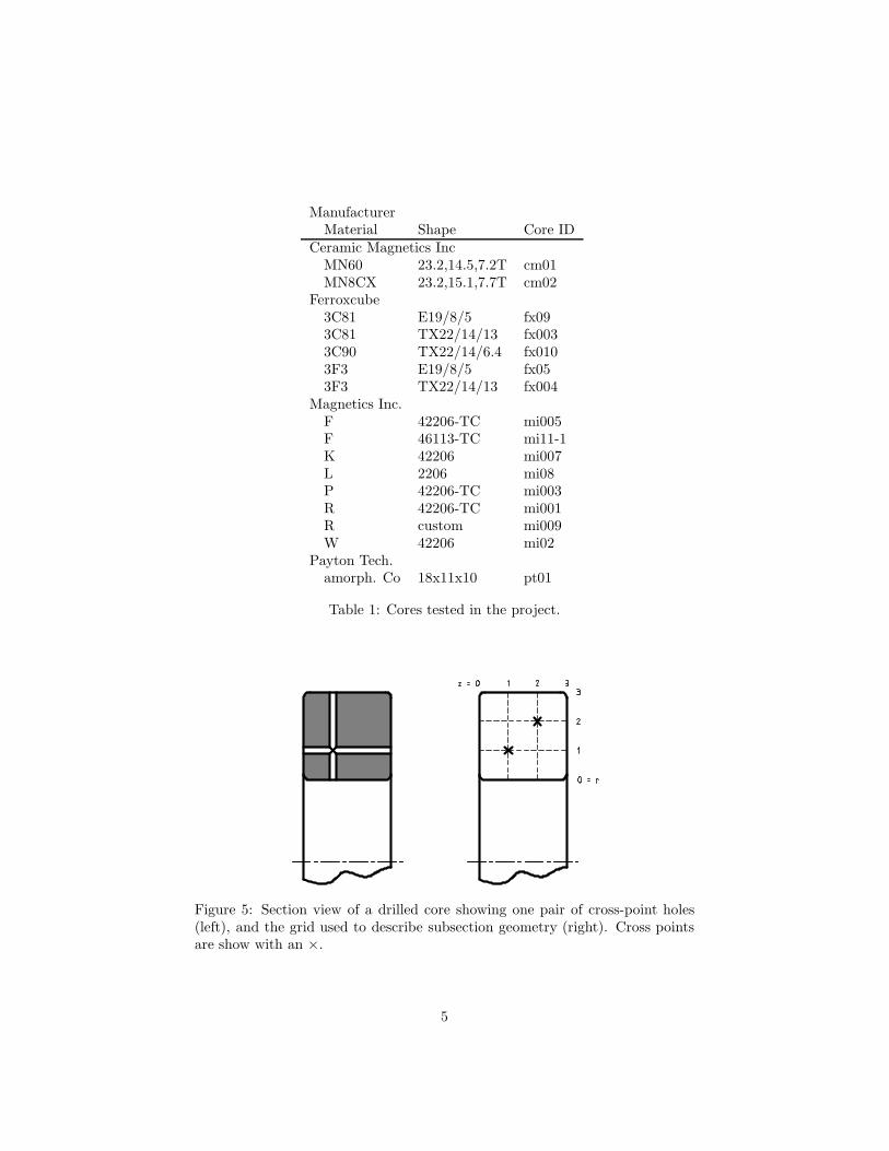
ManufacturerMaterial Shape Core ID

Ceramic Magnetics IncMN60 23.2,14.5,7.2T cm01MN8CX 23.2,15.1,7.7T cm02

Ferroxcube3C81 E19/8/5 fx093C81 TX22/14/13 fx0033C90 TX22/14/6.4 fx0103F3 E19/8/5 fx053F3 TX22/14/13 fx004

Magnetics Inc.F 42206-TC mi005F 46113-TC mi11-1K 42206 mi007L 2206 mi08P 42206-TC mi003R 42206-TC mi001R custom mi009W 42206 mi02

Payton Tech.amorph. Co 18x11x10 pt01

Table 1: Cores tested in the project.

Figure 5: Section view of a drilled core showing one pair of cross-point holes(left), and the grid used to describe subsection geometry (right). Cross pointsare show with an ×.

5

the toroid, to avoid unnecessary constriction of the flux path due to the holes.(The drawing is to scale; a single cross-point pair consumes 15% of the core crosssection area.) We take advantage of the symmetry of the toroid, and collapsethe circumferential dimension, regarding the cross points as lying in one radialcross-section plane (Figure 5, right). The details of the naming of subsections,necessary for interpreting the data, are presented in the user manual [2].

4.2 Experimental Setup

For these runs, the voltage across the embedded sense winding was recorded onan additional oscilloscope channel. The core had N = 4 turns for the primarywinding. By averaging over 512 triggers, the noise on the single-turn sense wind-ing was typically below the resolution of the oscilloscope digitization. Unlike theroutine runs, the center hole in the toroid was not blocked with a low-dielectric-constant material, in order to avoid fouling the probe holes. Measurements weremade at room temperature. Automatic degaussing was used (Section 7).

The sample was driven with square wave signals, and with the expand val-idation waveform. Our objective was to detect any unusual dynamic variationof the fraction of flux passing through the subsection, under these various driveconditions. We generated plots of three values: (1) the full-core sense windingvoltage, (2) the embedded winding voltage, and (3) the ratio of the two (Fig-ure 6). To make visual comparison easier, the embedded winding voltage wasscaled by NA/Ap, where N is the number of turns around the full cross-section,A is the full core cross-section area, and Ap is the “probe area,” the area of thecore enclosed within the sense winding. This ratio would be unity if the fluxdistribution were uniform.

Even under the null hypothesis that there are no new dynamic flux distri-bution effects discovered, and that the permeability is constant, uniform andisotropic, we would not expect the flux distribution be uniform—there is a ra-dial gradient, with B ∝ 1/r. The flux contained in the annulus between r1 andr2,

Φ(r1, r2) = h

∫ r1

r2

B(r)dr (1)

∝ log(r1)− log(r2) (2)

and h is the height of the toroid. For our drilled core,1 this leads us to expect(under the null hypothesis) ratios of 119%, 98.1%, and 83.4%, in that order,from inside out. The ratio in Figure 6 averages 116%.

Also, of the nine subsections, the four corner subsections have slightly lessarea, due to the corner radii, and will enclose less flux. The manufacturer doesnot specify this radius, and we did not measure it, being more interested in thedynamics of the flux distribution.

1Using the manufacturer’s nominal dimensions.

6

-0.3

-0.2

-0.1

0

0.1

0.2

0.3

0.4

-20 0 20 40 60 80 100 120-1

-0.5

0

0.5

1

1.5

2

2.5

3

Vol

ts p

er tu

rn

Rat

io

Time [µs]

Run mi11-1-010

TotalSection

Ratio

Figure 6: Flux distribution between subsections. The total flux is comparedwith the flux through the inner 1/3 annular section (designated 0031) of atoroidal core (the latter scaled by NA/Ap). The third plot is the ratio of thetwo.

4.3 Observations

We are looking for variations in the flux distribution with time, which shouldshow up as deviations of the sense winding voltage ratios from a constant. Suchdeviations could be caused by changes in the flux distribution in the core, or byspurious artifacts of the measurement apparatus. Careful examination of thedata can distinguish between the two.

In Figure 6 we see an interesting feature of the ratio plot—a transient atthe zero crossings. Figure 7 shows this more clearly, because here the periodis 8µs, instead of 120µs, and ringing at about 1.5MHz is easily seen. Thisringing appears in all the probe winding plots, but the outer, total-flux windingonly shows the 30MHz ringing characteristic of the drive circuitry. If the lowerfrequency ringing is due to flux migrating from one region to another, we expectthis lower frequency ringing to sum to zero across regions, and the polarity ofsome regions to be reversed.

Figure 8 shows the central annulus with the same excitation voltage, andwe see inverted low-frequency ringing. Figure 9 tells the whole story. In it,the probe winding voltages for all three annular layers of the core, and theirsum,2 are plotted together. The flux appears to move in and out of the centralregion from the other two regions. The lower frequency transients all cancel outin the sum of the three voltages, leaving only the high-frequency, drive circuitartifacts.

We believe the low frequency ringing is due to dimensional resonances, suchas described in [4], and are evident because of the low electromagnetic prop-agation velocity (v) of the ferrite medium. Because v is low, resonances due

2This is the sum of the three probe voltages, not the outer sense winding voltage, scaled.

7

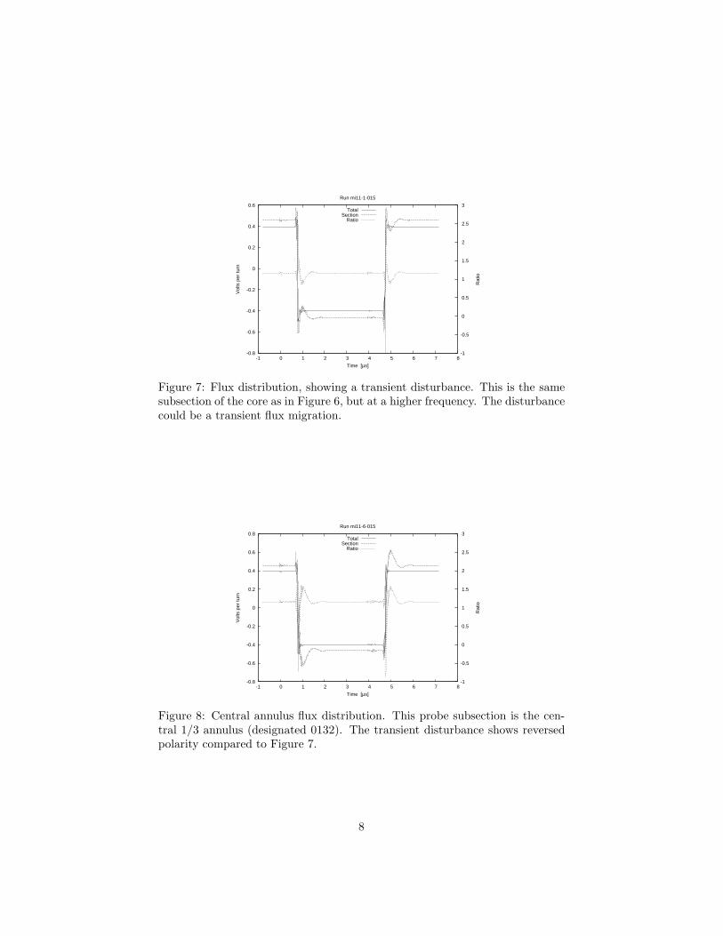
-0.8

-0.6

-0.4

-0.2

0

0.2

0.4

0.6

-1 0 1 2 3 4 5 6 7 8-1

-0.5

0

0.5

1

1.5

2

2.5

3

Vol

ts p

er tu

rn

Rat

io

Time [µs]

Run mi11-1-015

TotalSection

Ratio

Figure 7: Flux distribution, showing a transient disturbance. This is the samesubsection of the core as in Figure 6, but at a higher frequency. The disturbancecould be a transient flux migration.

-0.8

-0.6

-0.4

-0.2

0

0.2

0.4

0.6

0.8

-1 0 1 2 3 4 5 6 7 8-1

-0.5

0

0.5

1

1.5

2

2.5

3

Vol

ts p

er tu

rn

Rat

io

Time [µs]

Run mi11-6-015

TotalSection

Ratio

Figure 8: Central annulus flux distribution. This probe subsection is the cen-tral 1/3 annulus (designated 0132). The transient disturbance shows reversedpolarity compared to Figure 7.

8

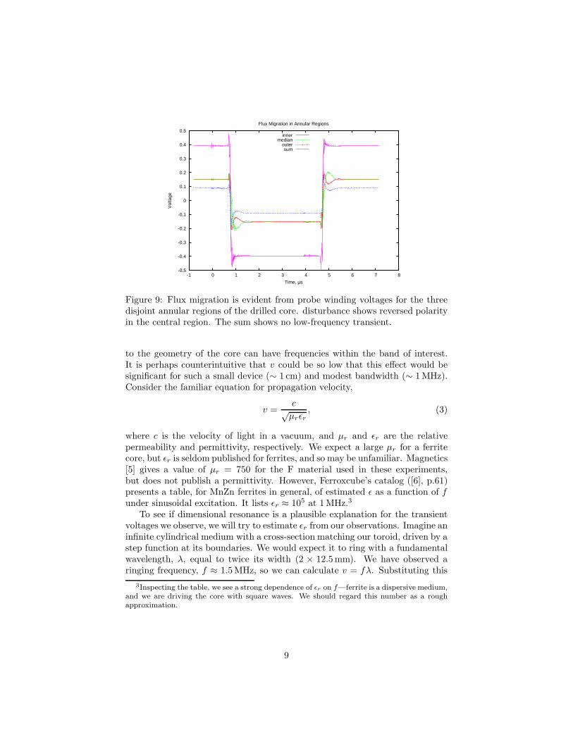
-0.5

-0.4

-0.3

-0.2

-0.1

0

0.1

0.2

0.3

0.4

0.5

-1 0 1 2 3 4 5 6 7 8

Vol

tage

Time, µs

Flux Migration in Annular Regions

innermedian

outersum

Figure 9: Flux migration is evident from probe winding voltages for the threedisjoint annular regions of the drilled core. disturbance shows reversed polarityin the central region. The sum shows no low-frequency transient.

to the geometry of the core can have frequencies within the band of interest.It is perhaps counterintuitive that v could be so low that this effect would besignificant for such a small device (∼ 1 cm) and modest bandwidth (∼ 1MHz).Consider the familiar equation for propagation velocity,

v =c

√µrǫr

, (3)

where c is the velocity of light in a vacuum, and µr and ǫr are the relativepermeability and permittivity, respectively. We expect a large µr for a ferritecore, but ǫr is seldom published for ferrites, and so may be unfamiliar. Magnetics[5] gives a value of µr = 750 for the F material used in these experiments,but does not publish a permittivity. However, Ferroxcube’s catalog ([6], p.61)presents a table, for MnZn ferrites in general, of estimated ǫ as a function of funder sinusoidal excitation. It lists ǫr ≈ 105 at 1MHz.3

To see if dimensional resonance is a plausible explanation for the transientvoltages we observe, we will try to estimate ǫr from our observations. Imagine aninfinite cylindrical medium with a cross-section matching our toroid, driven by astep function at its boundaries. We would expect it to ring with a fundamentalwavelength, λ, equal to twice its width (2 × 12.5mm). We have observed aringing frequency, f ≈ 1.5MHz, so we can calculate v = fλ. Substituting this

3Inspecting the table, we see a strong dependence of ǫr on f—ferrite is a dispersive medium,and we are driving the core with square waves. We should regard this number as a roughapproximation.

9

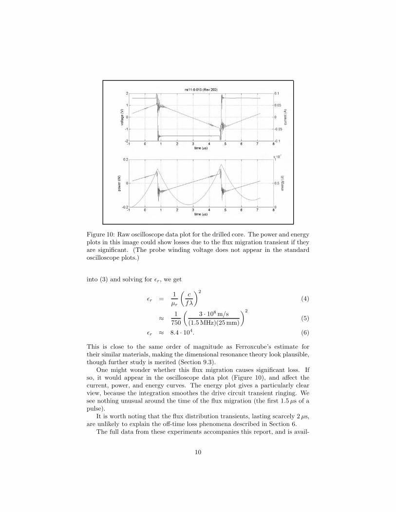
Figure 10: Raw oscilloscope data plot for the drilled core. The power and energyplots in this image could show losses due to the flux migration transient if theyare significant. (The probe winding voltage does not appear in the standardoscilloscope plots.)

into (3) and solving for ǫr, we get

ǫr =1

µr

(

c

fλ

)2

(4)

≈1

750

(

3 · 108m/s

(1.5MHz)(25mm)

)2

(5)

ǫr ≈ 8.4 · 104. (6)

This is close to the same order of magnitude as Ferroxcube’s estimate fortheir similar materials, making the dimensional resonance theory look plausible,though further study is merited (Section 9.3).

One might wonder whether this flux migration causes significant loss. Ifso, it would appear in the oscilloscope data plot (Figure 10), and affect thecurrent, power, and energy curves. The energy plot gives a particularly clearview, because the integration smoothes the drive circuit transient ringing. Wesee nothing unusual around the time of the flux migration (the first 1.5µs of apulse).

It is worth noting that the flux distribution transients, lasting scarcely 2µs,are unlikely to explain the off-time loss phenomena described in Section 6.

The full data from these experiments accompanies this report, and is avail-

10

able for further investigation of possible flux migration phenomena.

5 Steinmetz Curve Fits

The Steinmetz4 approximation,

Pv = kfαBβ , (7)

where Pv is the average power density, f is the excitation frequency, and B is thepeak flux density, is commonly used to characterize core loss data for sinusoidalexcitation, but can also be applied to our square-wave data. We first describea formulation in terms of frequency and flux density, but then also provide aformulation in terms of pulse widths and applied voltage.

To linearize the equation for curve fitting, we used base-10 logarithms (ref-erenced to 1V or 1 s), because the preferred values for voltage and time usedin the experiment are round decilog values, and because using log10 makesit convenient to express the standard error in familiar units of decibels (i.e.,10 log10(P/Pref)). This choice does not affect the values of the k, α, and βparameters.

In a typical case, Ferroxcube 3C81 material, fitting (7) to the entire set ofsquare wave data gave a standard error of about 1.5 dB. Visually inspectingthe plots shows a distinct increase in slope around 100 kHz. This inspired asix-parameter, two-plane curve fit,

Pv = max(k1fα1Bβ1 + k2f

α2Bβ2) (8)

This fits the data to two intersecting planes that function like a single plane witha fold in it (Figure 11). It fits the 3C81 data with a standard error of 0.35 dB,much better than the single equation, and also better than simply using differentparameters for different frequency ranges.

Note that while the formula we are fitting is essentially the same form asthe Steinmetz equation, and we use the variable names k, α, and β, this is adifferent model, because is is based on square wave experimental data, and isintended to predict rectangular pulse core losses. In situations where this mightcause confusion, we will subscript the present parameters5 to distinguish themfrom the classic Steinmetz, sinusoidal, parameters.

The boundary between the two planes (the fold) projected onto the log10(f)-log10(B) plane is a straight line,

log10(B) = a0 + a1 log10(f) (9)

where

a0 =log10(k1/k2)

β2 − β1

4Named for C.P. Steinmetz’s work [7], although Steinmetz did not include the frequencydependence that is now standard [8].

5We choose ‘r’, for “rectangular,” thus avoiding ‘s’ which might suggest either “square” or“sinusoidal.”

11

1

10

100

1000

10 100 1000

Loss

[m

W/c

m3 ]

Frequency [kHz]

Core Loss vs. Frequency with Two-plane Steinmetz Fit, Run Set fx003: Ferroxcube 3C81 Material

k1: 11.0126, α1: 1.31, β1: 2.61Std err: 0.034

k2: 6.5315e-005, α2: 2.18, β2: 2.11

rev 184.13

B^

[mT]155.798.262.039.124.715.69.8

Figure 11: Two-plane Steinmetz curve fit to Ferroxcube 3C81 material, squarewave loss data.

a1 =α1 − α2

β2 − β1.

The parameters a0 and a1 might provide a useful characterization of the tran-sition of the dominating loss mechanisms from hysteresis to eddy currents, forcomparing different materials. The two-plane Steinmetz parameters from ourexperiments are listed in Table 2.

This method of curve fitting has advantages over the common practice ofproviding independent Steinmetz parameters for different frequency ranges:

1. There is no step discontinuity at frequency range boundaries.

2. There is no arbitrary choice of boundary frequency. The curve-fittingoptimization chooses the best boundary line (i.e., choosing a0 and a1).

3. The curve fitting optimization uses all the data.

There is no significant computational penalty for using this model, and codingis easy; programmers can use either (8) directly, or (7), using k1, α1, and β1 forlog10(B) > a0 + a1 log10(f), and k2, α2, and β2 otherwise.

The two-plane Steinmetz parameters from our experiments are listed in Ta-ble 2. The table includes two different sets of k values. The lowercase k1 andk2 are the values used in (8), implicitly using reference values of 1 T and 1 Hz.Also listed are uppercase K1 and K2 based on reference values f0 = 100 kHz

12

ManufacturerMaterial Geom Set k1 K1 α1 β1 γ1 k2 K2 α2 β2 γ2

Ceramic Magnetics IncMN60 T cm01 6.085 86810 1.32 2.47 2.15 899.8µ 67879 2.00 2.13 1.13MN8CX T cm02 63.01 182100 1.19 2.49 2.3 177.4µ 87357 2.20 2.29 1.09

Ferroxcube3C81 T fx003 11.01 91200 1.31 2.61 2.3 65.32µ 41432 2.18 2.11 0.933C81 E fx09 18.02 88800 1.23 2.45 2.22 350.0µ 52769 2.10 2.33 1.233C90 T fx010 36.86 39570 1.19 2.94 2.75 2.895µ 18223 2.39 2.16 0.773F3 T fx004 102.4 67200 1.13 2.81 2.68 11.93µ 28414 2.30 2.14 0.843F3 E fx05 40.63 65950 1.14 2.50 2.36 224.8µ 38221 2.12 2.36 1.24

Magnetics Inc.F T mi005 26.41 72920 1.24 2.76 2.52 7.612µ 32369 2.37 2.22 0.85K T mi007 246.2 86830 1.10 2.95 2.85 5.276µ 20750 2.41 2.48 1.07L T mi08 706.8 150800 1.04 2.87 2.83 276.1m 99927 1.69 2.88 1.19P T mi003 10.91 43090 1.28 2.80 2.52 75.99µ 36099 2.16 2.13 0.97R T mi01-6 30.16 67220 1.25 2.90 2.65 14.55µ 30033 2.31 2.24 0.93W T mi02 832.7m 131000 1.51 2.37 1.86 10.59m 123857 1.82 2.04 1.22

Table 2: Two-plane Steinmetz parameters for various magnetic materials intwo general geometries, toroidal (T) and E-core (E). The ki parameters arereferenced to f = 1Hz and B = 1T; the Ki parameters are referenced tof = 100 kHz and B = 100mT. All the ki and Ki parameter have dimensions ofW/m3. The α and β parameters for use in (8); γ is required for (11).

and B0 = 100mT, to be used in

Pv = max(

K1(f/f0)α1(B/B0)

β1 +K2(f/f0)α2(B/B0)

β2

)

(10)

Both are included because the (8) is simpler to use, but the values of K1 andK2 are more physically meaningful, because they are based on results near therange of values used in practice, rather than on values many orders of magnitudedifferent.

For example, the values of K for one core shape are very similar to those foranother core shape and the same material, indicating that the losses predictedby the model are very similar for the two shapes. The values of k, on the otherhand, can be very different, but this is only an artifact of the use of the 1 T and1 Hz reference points, which are distant from the actual operating point, and isnot an indication that the predictions in the region of interest are significantlydifferent.

The results tend to indicate slightly smaller losses for E cores than for toroidalcores made with the same material. This does not actually indicate of superiorperformance for E cores. Rather, it is a result the effective area and effectivecore length provided one the core datasheet, which we used in our calculations.

13

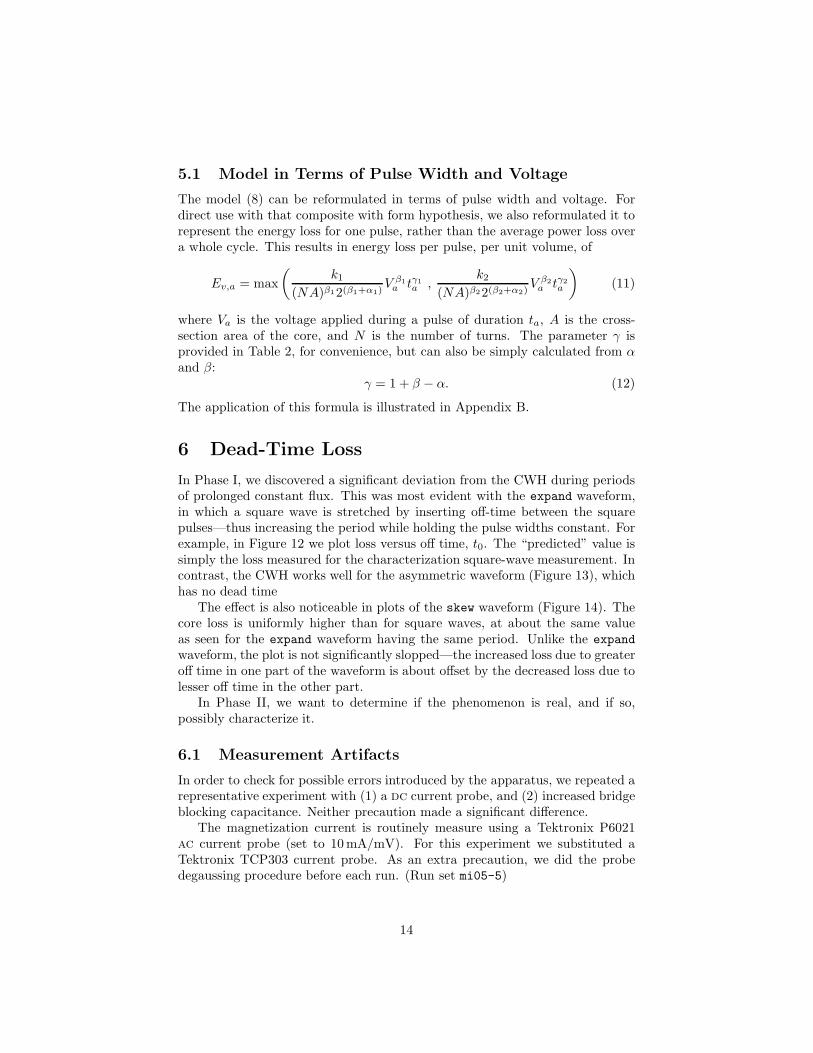
5.1 Model in Terms of Pulse Width and Voltage

The model (8) can be reformulated in terms of pulse width and voltage. Fordirect use with that composite with form hypothesis, we also reformulated it torepresent the energy loss for one pulse, rather than the average power loss overa whole cycle. This results in energy loss per pulse, per unit volume, of

Ev,a = max

(

k1(NA)β12(β1+α1)

V β1

a tγ1

a ,k2

(NA)β22(β2+α2)V β2

a tγ2

a

)

(11)

where Va is the voltage applied during a pulse of duration ta, A is the cross-section area of the core, and N is the number of turns. The parameter γ isprovided in Table 2, for convenience, but can also be simply calculated from αand β:

γ = 1 + β − α. (12)

The application of this formula is illustrated in Appendix B.

6 Dead-Time Loss

In Phase I, we discovered a significant deviation from the CWH during periodsof prolonged constant flux. This was most evident with the expand waveform,in which a square wave is stretched by inserting off-time between the squarepulses—thus increasing the period while holding the pulse widths constant. Forexample, in Figure 12 we plot loss versus off time, t0. The “predicted” value issimply the loss measured for the characterization square-wave measurement. Incontrast, the CWH works well for the asymmetric waveform (Figure 13), whichhas no dead time

The effect is also noticeable in plots of the skew waveform (Figure 14). Thecore loss is uniformly higher than for square waves, at about the same valueas seen for the expand waveform having the same period. Unlike the expand

waveform, the plot is not significantly slopped—the increased loss due to greateroff time in one part of the waveform is about offset by the decreased loss due tolesser off time in the other part.

In Phase II, we want to determine if the phenomenon is real, and if so,possibly characterize it.

6.1 Measurement Artifacts

In order to check for possible errors introduced by the apparatus, we repeated arepresentative experiment with (1) a dc current probe, and (2) increased bridgeblocking capacitance. Neither precaution made a significant difference.

The magnetization current is routinely measure using a Tektronix P6021ac current probe (set to 10mA/mV). For this experiment we substituted aTektronix TCP303 current probe. As an extra precaution, we did the probedegaussing procedure before each run. (Run set mi05-5)

14

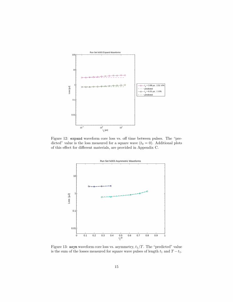
10−1

100

101

0.01

0.1

1

10

100

t0 [µs]

Loss

[µJ]

Run Set fx003 Expand Waveforms

t1 = 3.98 µs; 2.51 V/N

predictedt1 = 6.31 µs; 1 V/N

predicted

Figure 12: expand waveform core loss vs. off time between pulses. The “pre-dicted” value is the loss measured for a square wave (t0 = 0). Additional plotsof this effect for different materials, are provided in Appendix C.

0 0.1 0.2 0.3 0.4 0.5 0.6 0.7 0.8 0.9 1

0.01

0.1

1

10

t1/T

Loss

[µJ

]

Run Set fx003 Asymmetric Waveforms

Figure 13: asym waveform core loss vs. asymmetry, t1/T . The “predicted” valueis the sum of the losses measured for square wave pulses of length t1 and T − t1.

15

100

101

0.01

0.1

1

10

t0 [µs]

loss

[µJ

]

fx003 Skew Waveforms

t1 = 3.98 µs; 2.51 V/N

predictedt1 = 6.31 µs; 1 V/N

predicted

Figure 14: skew core loss vs. t0, where t0 is the off time between the first andsecond pulses. The other off time equals T − 2t1 − t0

.

In Phase I, the bridge was equipped with a 320µF blocking capacitor. Onvery long expand runs, low-frequency ringing was evident. We wanted to im-prove this performance by increasing the blocking capacitance, while loweringthe effective series resistance, so we installed 120mF of blocking capacitance,using Epcos MKT series polyester capacitors.

6.2 Zero-Flux Off Time

In order to see if the extra loss is correlated with the presence of magnetic flux,we devised a new wave form, the hippo (Figure 3), named for its resemblanceto hippopotamus dentition. This waveform has two pairs of pulses, with eachpair having a width of t1 (i.e., two opposing pulses of width t1/2). Thus theflux returns to zero during the off time. Using this waveform, the measured lossmatched the predicted value more closely, actually dropping somewhat (Fig-ure 15). 6

6We also note a curious hump in the plot at very low t0. This is an artifact of theapparatus—the waveform decoder circuitry ([1], Section 4) has a delay of about 400 ns in theOUT signal rise time, making unable to create this short a dead time for the hippo waveform.The plot time scale is based on the SYNC signal, not the actual sense winding voltage.

16

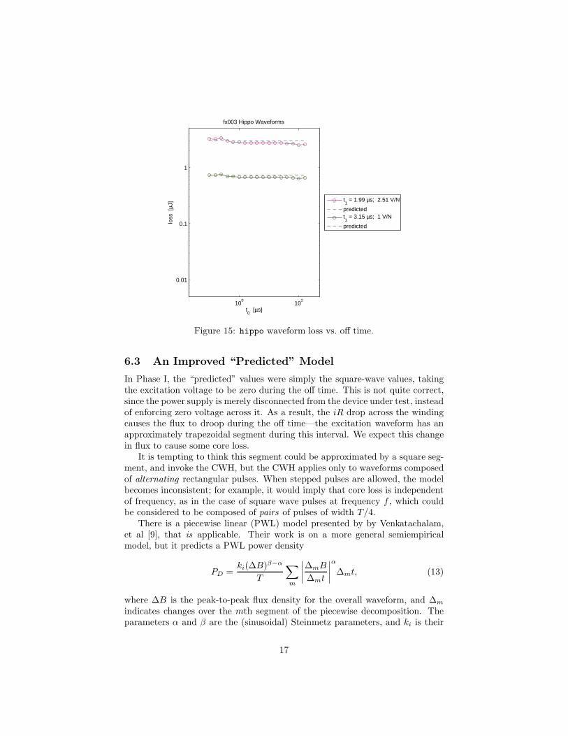
100

102

0.01

0.1

1

t0 [µs]

loss

[µJ

]

fx003 Hippo Waveforms

t1 = 1.99 µs; 2.51 V/N

predictedt1 = 3.15 µs; 1 V/N

predicted

Figure 15: hippo waveform loss vs. off time.

6.3 An Improved “Predicted” Model

In Phase I, the “predicted” values were simply the square-wave values, takingthe excitation voltage to be zero during the off time. This is not quite correct,since the power supply is merely disconnected from the device under test, insteadof enforcing zero voltage across it. As a result, the iR drop across the windingcauses the flux to droop during the off time—the excitation waveform has anapproximately trapezoidal segment during this interval. We expect this changein flux to cause some core loss.

It is tempting to think this segment could be approximated by a square seg-ment, and invoke the CWH, but the CWH applies only to waveforms composedof alternating rectangular pulses. When stepped pulses are allowed, the modelbecomes inconsistent; for example, it would imply that core loss is independentof frequency, as in the case of square wave pulses at frequency f , which couldbe considered to be composed of pairs of pulses of width T/4.

There is a piecewise linear (PWL) model presented by by Venkatachalam,et al [9], that is applicable. Their work is on a more general semiempiricalmodel, but it predicts a PWL power density

PD =ki(∆B)β−α

T

∑

m

∣

∣

∣

∣

∆mB

∆mt

∣

∣

∣

∣

α

∆mt, (13)

where ∆B is the peak-to-peak flux density for the overall waveform, and ∆m

indicates changes over the mth segment of the piecewise decomposition. Theparameters α and β are the (sinusoidal) Steinmetz parameters, and ki is their

17

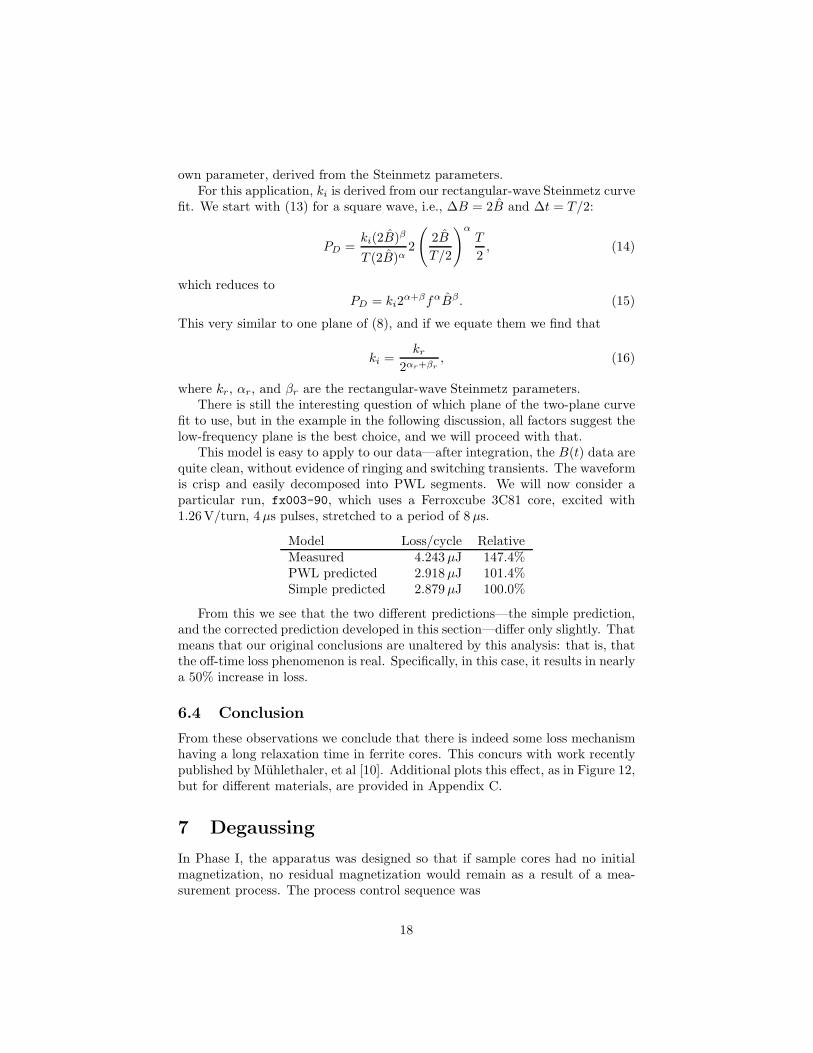
own parameter, derived from the Steinmetz parameters.For this application, ki is derived from our rectangular-wave Steinmetz curve

fit. We start with (13) for a square wave, i.e., ∆B = 2B and ∆t = T/2:

PD =ki(2B)β

T (2B)α2

(

2B

T/2

)αT

2, (14)

which reduces toPD = ki2

α+βfαBβ. (15)

This very similar to one plane of (8), and if we equate them we find that

ki =kr

2αr+βr

, (16)

where kr, αr, and βr are the rectangular-wave Steinmetz parameters.There is still the interesting question of which plane of the two-plane curve

fit to use, but in the example in the following discussion, all factors suggest thelow-frequency plane is the best choice, and we will proceed with that.

This model is easy to apply to our data—after integration, the B(t) data arequite clean, without evidence of ringing and switching transients. The waveformis crisp and easily decomposed into PWL segments. We will now consider aparticular run, fx003-90, which uses a Ferroxcube 3C81 core, excited with1.26V/turn, 4µs pulses, stretched to a period of 8µs.

Model Loss/cycle RelativeMeasured 4.243µJ 147.4%PWL predicted 2.918µJ 101.4%Simple predicted 2.879µJ 100.0%

From this we see that the two different predictions—the simple prediction,and the corrected prediction developed in this section—differ only slightly. Thatmeans that our original conclusions are unaltered by this analysis: that is, thatthe off-time loss phenomenon is real. Specifically, in this case, it results in nearlya 50% increase in loss.

6.4 Conclusion

From these observations we conclude that there is indeed some loss mechanismhaving a long relaxation time in ferrite cores. This concurs with work recentlypublished by Muhlethaler, et al [10]. Additional plots this effect, as in Figure 12,but for different materials, are provided in Appendix C.

7 Degaussing

In Phase I, the apparatus was designed so that if sample cores had no initialmagnetization, no residual magnetization would remain as a result of a mea-surement process. The process control sequence was

18

1. Set up and run the pulse timing logic signal (before turning on the bridgepower supply; the function generator is always on).

2. Upload the required voltage to the bridge power supply.

3. Enable the power supply output.

4. After a delay, initiate the oscilloscope data acquisition sequence.

5. After the oscilloscope signals that data acquisition is complete, disable thepower supply output; the voltage slews to zero at about 1.5V/s. This slewrate is not programmable—it is just a property of the particular powersupply we are using.

6. Delay several seconds to allow the power supply to settle and the core tocool.

However, there was some concern that there might still be some residualmagnetization, either initially, in the core as supplied by the manufacturer, orintroduced inadvertently, in the handling of the wound device, or due to anundiscovered defect in the apparatus or its control algorithm.

To check for this possibility, we created a degaussing control sequence, reransome experiments and compared the results with those obtained with the orig-inal setup. The new control sequence was

1. Setup and run the pulse timing logic signal.

2. Upload the maximum safe voltage to the bridge power supply and enablethe power supply output. The voltage slews from zero to the maximumvoltage, driving the core into saturation.

3. Upload the voltage required for the experiment. The output voltage slewsdown to that value at about 1.5V/s. This is the degaussing step.

4. When the power supply output voltage reaches the correct value, initiatethe oscilloscope data acquisition sequence.

5. After the oscilloscope signals that data acquisition is complete, disable thepower supply output.

6. Delay for power supply settling and core cooling.

With this degaussing scheme, the residual flux for a square wave is limitedto about T 2r/2, where T is the period and r is the slew rate. At 10 kHz, thisworks out to about 8 nWb per turn.

This control sequence adds significantly to the overall run time for a sample,due to the degaussing voltage decay time. To speed things up, we switched froma worst-case, fixed delay (step 4 of the old sequence), to an adaptive delay thatonly waits long enough for the output voltage to reach its target.

Comparing the results we saw no significant difference. This makes us moreconfident, but it is not a conclusive result. A better approach might be to

19

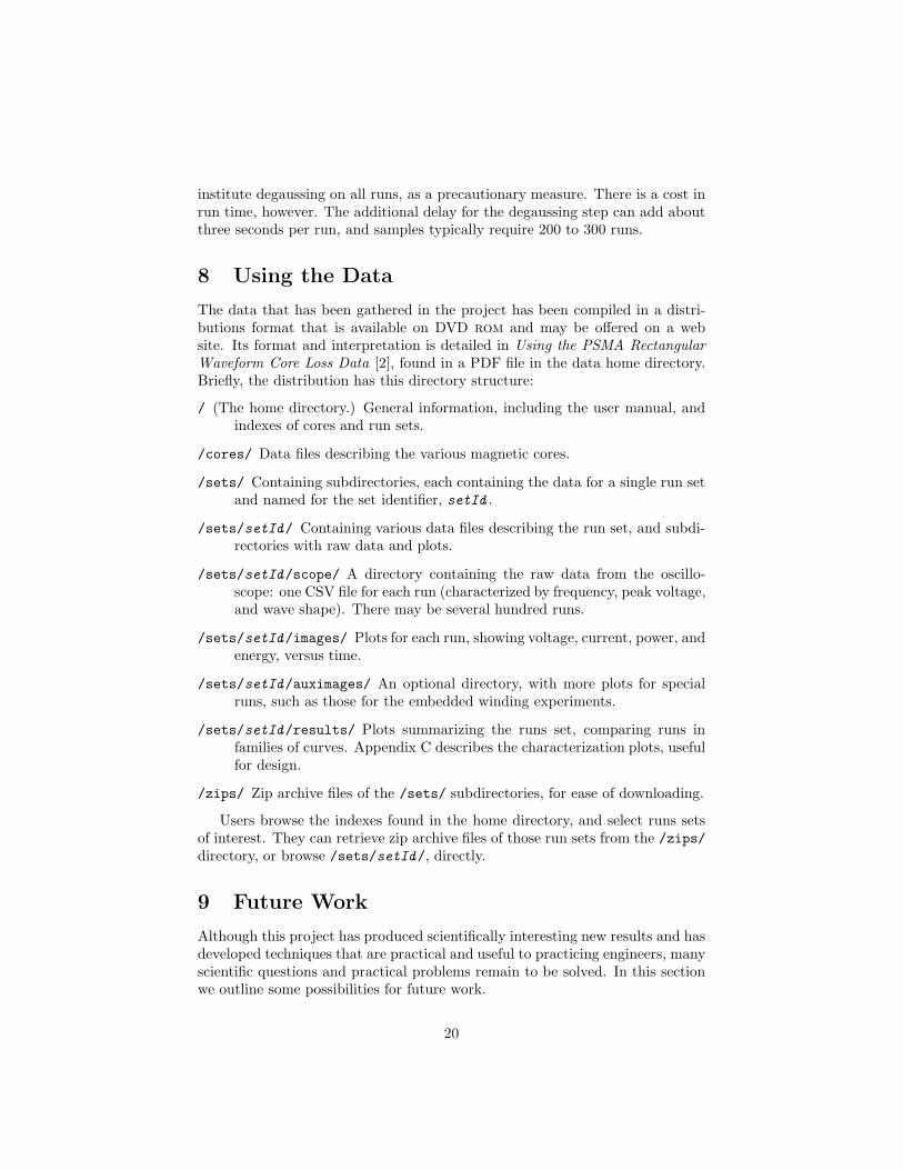
institute degaussing on all runs, as a precautionary measure. There is a cost inrun time, however. The additional delay for the degaussing step can add aboutthree seconds per run, and samples typically require 200 to 300 runs.

8 Using the Data

The data that has been gathered in the project has been compiled in a distri-butions format that is available on DVD rom and may be offered on a website. Its format and interpretation is detailed in Using the PSMA RectangularWaveform Core Loss Data [2], found in a PDF file in the data home directory.Briefly, the distribution has this directory structure:

/ (The home directory.) General information, including the user manual, andindexes of cores and run sets.

/cores/ Data files describing the various magnetic cores.

/sets/ Containing subdirectories, each containing the data for a single run setand named for the set identifier, setId .

/sets/setId/ Containing various data files describing the run set, and subdi-rectories with raw data and plots.

/sets/setId/scope/ A directory containing the raw data from the oscillo-scope: one CSV file for each run (characterized by frequency, peak voltage,and wave shape). There may be several hundred runs.

/sets/setId/images/ Plots for each run, showing voltage, current, power, andenergy, versus time.

/sets/setId/auximages/ An optional directory, with more plots for specialruns, such as those for the embedded winding experiments.

/sets/setId/results/ Plots summarizing the runs set, comparing runs infamilies of curves. Appendix C describes the characterization plots, usefulfor design.

/zips/ Zip archive files of the /sets/ subdirectories, for ease of downloading.

Users browse the indexes found in the home directory, and select runs setsof interest. They can retrieve zip archive files of those run sets from the /zips/directory, or browse /sets/setId/, directly.

9 Future Work

Although this project has produced scientifically interesting new results and hasdeveloped techniques that are practical and useful to practicing engineers, manyscientific questions and practical problems remain to be solved. In this sectionwe outline some possibilities for future work.

20

9.1 Modeling

The model developed here provides improved accuracy in modeling core lossacross a wide range of practical waveforms and frequencies. However, there arethree important limits on its applicability:

• It does not account for the effects of dc flux bias in the core.

• It does not account for the off-time loss phenomenon.

• It provides a method for calculation of loss from a set of excitation wave-forms, but does not provide a dynamic model applicable to simulation ofa component, circuit, or system in a Spice or other computer simulation.

Although there has been work published addressing the effects of dc bias andattempting to model the off-time loss phenomenon, it is not clear that theavailable approaches are practical or that they will work consistently across awide range of excitation parameters, such as the data collected here. There isalso a range of simulation models available for hysteretic behavior. However,most of these models address only static (rate-independent) hysteresis, and donot begin to capture the frequency and waveform dependence captured in themodels and data we have developed. Work is needed on all three issues. Thedata collected in Phase II provides a rich resource for such work. For example,one would want to ensure that models developed provided results for the hippowaveform consistent with the data.

9.2 Hardware

Further hardware development may be considered for the purposes of developingcapabilities beyond those of the equipment used in this work, and for developingequipment that is practical for routine square-wave core-loss measurement bycore manufacturers and by core users.

The maximum frequency used in our testing was 500 kHz. Although appli-cations at higher frequency are limited, rapid progress in wide-bandgap semi-conductors is generating increased interest in switching frequencies in the MHzrange. In addition, testing at higher frequencies could help ensure that themodeling provides accurate results for any waveform. Improvements in switch-ing speed and stray impedances that would be needed to increase the frequencyof operation would simultaneously increase the fidelity of waveforms and providemore accurate results near 500 kHz.

Now that the applicability of square-wave testing has been demonstrated,core manufacturers and by core users may wish to develop their own capabilityfor this type of measurement. This calls for an easily replicable test setup usingcommercially available components, perhaps with some custom-made compo-nents.

21

9.3 Flux Spatial Dynamics

A small set of drilled-core measurements has shown that the flux distributionis not uniform across a core throughout a switching cycle. We hypothesizethat the flux migration we see is consistent with the dimensional resonanceeffects analyzed in detail in [4]. In order to verify this, the dielectric constantof the material used needs to be measured. With this parameter, it would bepossible to develop a simulation of expected behavior in the scenario we tested,to verify that what we observed can be attributed to this phenomenon. Anotherverification approach would be to repeat the drilled-core tests with sinusoidalexcitation for which modeling is easier. If the behaviors do not agree, additionaltheoretical and experimental investigations would be called for.

Although [4] provides guidelines for determining when dimensional reso-nance effects become important, and approaches for calculating the effects whenthey are important, the analysis assumes sine-wave excitation. More work isneeded to fully understand the implications of dimensional resonance effectswith square-wave and other non-sinusoidal waveforms.

9.4 Design Implications

The most important implication of the data collection and modeling we per-formed for design work is that it is now possible to design a magnetic componentand have fewer surprises about its loss behavior in a power electronics applica-tion. Having accurate models also allows employing computer optimization ofdesigns.

Some of the design implications of the square wave loss data can be under-stood when the data is plotted in a Herbert plot as discussed in [11]. However,that discussion does not take into account the off-time loss phenomenon, or thedifferent loss results obtained with the hippo waveform. Further work is neededto fully explore the design implications of these effects.

10 Conclusion

Together with the work in Phase I of this project, this work has greatly improvedour understanding of core loss with non-sinusoidal waveforms. A key result isa simple approach to predict losses for various rectangular voltage waveforms.These calculations can be performed based on parameters we provide for mate-rials we have measured, or can be based on simple square-wave measurementsof other materials. An additional outcome of this work is a large data set of lossmeasurements for a wide variety of materials and waveforms that can be usedfor future study in this area.

A key component of this work was the evaluation of the composite waveformhypothesis, which allows analyzing the loss for various rectangular waveformsbased on data taken for only square-wave excitation. This approach has beenshown to be effective, and can be expected to give more accurate results thanprevious approaches.

22

Our detailed investigation of the composite waveform hypothesis uncovered aphenomenon in which the per-cycle losses increase with increasing “dead time”during which the core sits with a constant, elevated flux level. Further in-vestigation of this has confirmed that it is a real effect, and it has generatedinternational attention, with experiments by another group confirming the phe-nomenon we discovered. An approach to predicting loss including this effect hasbeen proposed in [10]. Future work could develop better understanding of thephenomenon and easier approaches to predicting behavior considering it.

We also investigated the time dependence of the flux distribution throughdifferent regions of the core, both vertically and horizontally. We see transientoscillations of flux distribution that probably indicates the existence of standingwaves due to low electromagnetic propagation velocity due to the high perme-ability and permittivity of the ferrite material. There is no indication that thisis a significant loss mechanism for the experimental configuration, nor that ithas any relevance for the dead-time loss anomalies.

This does not exclude the possibility that there are dynamic flux distributioneffects at the micro or nano scale, but only shows that those we can detect onthe scale of these experiments are not involved in a significant loss mechanism.

Three results of this work can readily be applied in practice. The firstis predicting loss for any rectangular waveform using data from square-wavemeasurements. The second is using a two-plane Steinmetz model to fit this dataover a wide frequency range. The third is the set of parameters for this modelthat we provide in Table 2 for the particular materials that we measured. Anexample and tutorial for using these parameters to predict loss with rectangularwaveforms is provided in Appendix B.

23

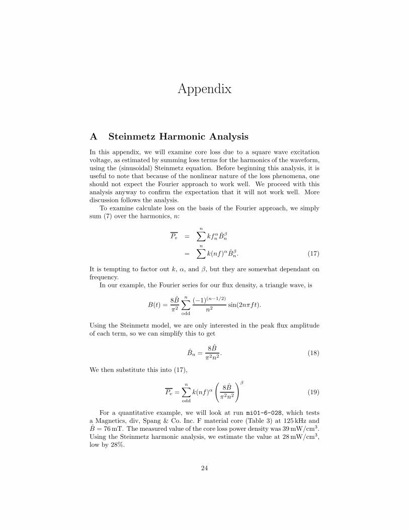
Appendix

A Steinmetz Harmonic Analysis

In this appendix, we will examine core loss due to a square wave excitationvoltage, as estimated by summing loss terms for the harmonics of the waveform,using the (sinusoidal) Steinmetz equation. Before beginning this analysis, it isuseful to note that because of the nonlinear nature of the loss phenomena, oneshould not expect the Fourier approach to work well. We proceed with thisanalysis anyway to confirm the expectation that it will not work well. Morediscussion follows the analysis.

To examine calculate loss on the basis of the Fourier approach, we simplysum (7) over the harmonics, n:

Pv =

n∑

kfαn B

βn

=

n∑

k(nf)αBβn . (17)

It is tempting to factor out k, α, and β, but they are somewhat dependant onfrequency.

In our example, the Fourier series for our flux density, a triangle wave, is

B(t) =8B

π2

n∑

odd

(−1)(n−1/2)

n2sin(2nπft).

Using the Steinmetz model, we are only interested in the peak flux amplitudeof each term, so we can simplify this to get

Bn =8B

π2n2. (18)

We then substitute this into (17),

Pv =

n∑

odd

k(nf)α

(

8B

π2n2

)β

(19)

For a quantitative example, we will look at run mi01-6-028, which testsa Magnetics, div, Spang & Co. Inc. F material core (Table 3) at 125 kHz andB = 76mT. The measured value of the core loss power density was 39mW/cm3.Using the Steinmetz harmonic analysis, we estimate the value at 28mW/cm3,low by 28%.

24

Parameter Value for f above0 kHz 100 kHz 500 kHz

k 0.074 0.036 0.014α 1.43 1.64 1.84β 2.85 2.68 2.28

Table 3: Published Steinmetz parameters for Magnetics Div., Spang & Co. Rmaterial [12]. Frequencies are referenced to 1 kHz, flux density to 1 kG, andPv [=] mW/cm2.

The failure of the harmonic analysis based on Fourier series to predict theloss accurately may be understood based on the nonlinear nature of the core loss.For linear phenomena such as resistive losses in windings or other conductors,in which loss is proportional to the square of the excitation amplitude, the losscalculated based on the Fourier decomposition can be mathematically proven tobe identical to the loss calculated directly from the original waveform. However,this does not hold for a nonlinear system. Particularly in the lower end of thefrequency range of interest, the Steinmetz parameters in Table 11 show that thepower loss is proportional to the flux density to a power significantly greaterthan two, typically in the range of 2.4 to 3. On this basis, one can expect thatwhen the full flux is considered together the loss will be higher than that thatwould be predicted based on the individual components considered separately.That is what we see in the results above.

Another experiment that illustrates the futility of using a Fourier decompo-sition to accurately predict core loss is described in [13]. A waveform consistingof a fundamental and a third harmonic is synthesized, and applied to a coreunder test. Varying the phase of the third harmonic has a significant effect onthe loss. A Fourier decomposition could not capture this effect.

25

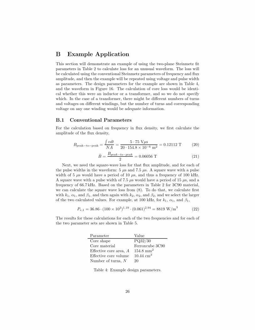
B Example Application

This section will demonstrate an example of using the two-plane Steinmetz fitparameters in Table 2 to calculate loss for an unusual waveform. The loss willbe calculated using the conventional Steinmetz parameters of frequency and fluxamplitude, and then the example will be repeated using voltage and pulse widthas parameters. The design parameters for the example are shown in Table 4,and the waveform in Figure 16. The calculation of core loss would be identi-cal whether this were an inductor or a transformer, and so we do not specifywhich. In the case of a transformer, there might be different numbers of turnsand voltages on different windings, but the number of turns and correspondingvoltage on any one winding would be adequate information.

B.1 Conventional Parameters

For the calculation based on frequency in flux density, we first calculate theamplitude of the flux density,

Bpeak−to−peak =

∫

vdt

NA=

5 · 75 Vµs

20 · 154.8× 10−6 m2= 0.12112 T (20)

B =Bpeak−to−peak

2= 0.06056 T (21)

Next, we need the square-wave loss for that flux amplitude, and for each ofthe pulse widths in the waveform: 5 µs and 7.5 µs. A square wave with a pulsewidth of 5 µs would have a period of 10 µs, and thus a frequency of 100 kHz.A square wave with a pulse width of 7.5 µs would have a period of 15 µs, and afrequency of 66.7 kHz. Based on the parameters in Table 2 for 3C90 material,we can calculate the square wave loss from (8). To do that, we calculate firstwith k1, α1, and β1, and then again with k2, α2, and β2, and we select the largerof the two calculated values. For example, at 100 kHz, for k1, α1, and β1,

Pv,1 = 36.86 · (100× 103)1.19 · (0.061)2.94 = 8819 W/m3

(22)

The results for these calculations for each of the two frequencies and for each ofthe two parameter sets are shown in Table 5.

Parameter ValueCore shape PQ32/30Core material Ferroxcube 3C90Effective core area, A 154.8 mm2

Effective core volume 10.44 cm3

Number of turns, N 20

Table 4: Example design parameters.

26

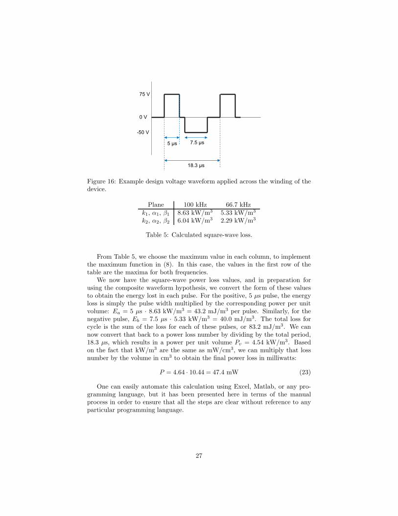
Figure 16: Example design voltage waveform applied across the winding of thedevice.

Plane 100 kHz 66.7 kHzk1, α1, β1 8.63 kW/m3 5.33 kW/m3

k2, α2, β2 6.04 kW/m3 2.29 kW/m3

Table 5: Calculated square-wave loss.

From Table 5, we choose the maximum value in each column, to implementthe maximum function in (8). In this case, the values in the first row of thetable are the maxima for both frequencies.

We now have the square-wave power loss values, and in preparation forusing the composite waveform hypothesis, we convert the form of these valuesto obtain the energy lost in each pulse. For the positive, 5 µs pulse, the energyloss is simply the pulse width multiplied by the corresponding power per unitvolume: Ea = 5 µs · 8.63 kW/m3 = 43.2 mJ/m3 per pulse. Similarly, for thenegative pulse, Eb = 7.5 µs · 5.33 kW/m3 = 40.0 mJ/m3. The total loss forcycle is the sum of the loss for each of these pulses, or 83.2 mJ/m3. We cannow convert that back to a power loss number by dividing by the total period,18.3 µs, which results in a power per unit volume Pv = 4.54 kW/m3. Basedon the fact that kW/m3 are the same as mW/cm3, we can multiply that lossnumber by the volume in cm3 to obtain the final power loss in milliwatts:

P = 4.64 · 10.44 = 47.4 mW (23)

One can easily automate this calculation using Excel, Matlab, or any pro-gramming language, but it has been presented here in terms of the manualprocess in order to ensure that all the steps are clear without reference to anyparticular programming language.

27

B.2 Pulse width and Voltage as Parameters

In this case, we directly apply (11), repeated here for convenience:

Ev,a = max

(

k1(NA)β12(β1+α1)

V β1

a tγ1

a ,k2

(NA)β22(β2+α2)V β2

a tγ2

a

)

(24)

We substitute in values from Table 4 and values of parameters k1 = 36.86,α1 = 1.19, beta1 = 2.94 and γ1 = 2.75 for the first set and k2 = 2.895, α2 = 2.39,beta2 = 2.16 and γ2 = 2.77 for the second. We obtain, for 5 µs and 75 V,Ev,a = 43.2 mJ/m3, and, for 7.5 µs and 50 V, Ev,b = 40.0 mJ/m3, exactly thesame as was found with the other approach. Any difference would only occuras a result of roundoff errors tracking through the calculation.

As before, the total loss for cycle is the sum of the loss for each of thesepulses, or 83.2 mJ/m3. We can now convert that back to a power loss numberby dividing by the total period, 18.3 µs, which results in a power per unit volumePv = 4.54 kW/m3, and an average power loss of 47.4 mW.

28

C Characterization Plots

Various plots have been provided with the data (Section 8) for visualizing thecharacterization (square wave) data. We present example plots in this appendix.For a more detailed explanation, see the user manual [2]. Image file names havethe form type conven-setId.ext , where type is the type of plot, setId is therun set identifier, and .ext is the graphics file extension.

C.1 Conventional Core Loss Plots

Conventional plots of core loss versus B are provided. These are similar to theloss plots provided by manufacturers for sinusoidal excitation, but are for oursquare wave data.

Image file names have the form conven-setId.ext .

29

C.2 Herbert Curves

Herbert plots (Figure 17) show core loss versus pulse width, t1, parameterizedby B. Herbert [3] describes their use in design.

Image file names have the form conven-setId.ext .

1 100 1

0.001

0.01

0.1

1

10

t1 (µs)

Loss

(W

)

Run Set fx003 Herbert Curves

3.98 V/N2.51 V/N1.59 V/N1 V/N0.63 V/N0.4 V/N

Figure 17: Herbert plot for Ferroxcube 3C81 material.

30

C.3 Hysteresis Plots

Hysteresis plots are provided for the characterisation square-wave data (Fig-ure 18). The plots are presented in families of constant pulse width, varyingB. Because of ringing in the sense voltage signal due to limitation in the appa-ratus, simply plotting B versus H gives a messy plot, with the hysteresis loopshape obscured by the ringing. We use boxcar averaging, tuned to the ringingfrequency (with a 85.3µs window) to drop out the ringing. These plots do nothave long saturation tails, partly because of this filtering, but also because theexperiments did not generally drive the cores deep into saturation.

Image file names have the form hyst-setId-Tset.ext , where Tset is thepulse width family identifier.

-200

-150

-100

-50

0

50

100

150

200

-25 -20 -15 -10 -5 0 5 10 15 20 25

B [m

T]

H [A/m]

Run Set fx003 Hysteresis, T = 20.0 µs Ferroxcube 3C81 material

fx003-006fx003-015fx003-023fx003-030

Figure 18: Hysteresis plot for Ferroxcube 3C81 material square wave data, 10µspulses. The legend gives the run identifiers, but these are not needed, as theonly difference between the loops shown is the amplitude of excitation, and thevalue of B can be read from the plot.

31

D Expand Plots

In this appendix we present the expand waveform loss versus off-time plots forall the core materials tested.

10−1

100

101

0.01

0.1

1

10

100

t0 [µs]

Loss

[µJ]

Run Set cm01 Expand Waveforms

t1 = 15.85 µs; 1 V/N

predictedt1 = 3.98 µs; 1 V/N

predictedt1 = 1 µs; 1 V/N

predictedt1 = 15.85 µs; 0.25 V/N

predictedt1 = 3.98 µs; 0.25 V/N

predictedt1 = 1 µs; 0.25 V/N

predicted

Figure 19: expand core loss vs. off-time for Ceramic Magnetics MN60.

10−1

100

101

0.01

0.1

1

10

100

t0 [µs]

Loss

[µJ]

Run Set cm02 Expand Waveforms

t1 = 15.85 µs; 1 V/N

predictedt1 = 3.98 µs; 1 V/N

predictedt1 = 1 µs; 1 V/N

predictedt1 = 15.85 µs; 0.25 V/N

predictedt1 = 3.98 µs; 0.25 V/N

predictedt1 = 1 µs; 0.25 V/N

predicted

Figure 20: expand core loss vs. off-time for Ceramic Magnetics MN8CX.

32

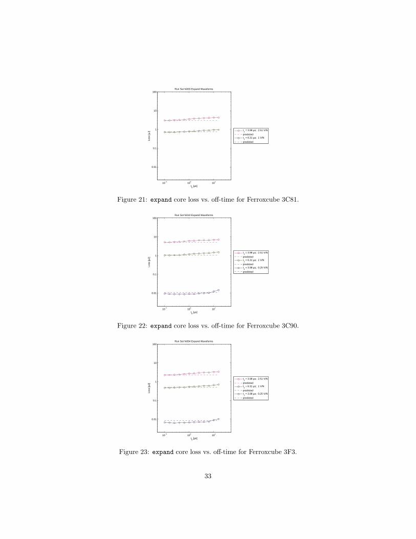
10−1

100

101

0.01

0.1

1

10

100

t0 [µs]

Loss

[µJ]

Run Set fx003 Expand Waveforms

t1 = 3.98 µs; 2.51 V/N

predictedt1 = 6.31 µs; 1 V/N

predicted

Figure 21: expand core loss vs. off-time for Ferroxcube 3C81.

10−1

100

101

0.01

0.1

1

10

100

t0 [µs]

Loss

[µJ]

Run Set fx010 Expand Waveforms

t1 = 3.98 µs; 2.51 V/N

predictedt1 = 6.31 µs; 1 V/N

predictedt1 = 3.98 µs; 0.25 V/N

predicted

Figure 22: expand core loss vs. off-time for Ferroxcube 3C90.

10−1

100

101

0.01

0.1

1

10

100

t0 [µs]

Loss

[µJ]

Run Set fx004 Expand Waveforms

t1 = 3.98 µs; 2.51 V/N

predictedt1 = 6.31 µs; 1 V/N

predictedt1 = 3.98 µs; 0.25 V/N

predicted

Figure 23: expand core loss vs. off-time for Ferroxcube 3F3.

33

10−1

100

101

0.01

0.1

1

10

100

t0 [µs]

Loss

[µJ]

Run Set mi005 Expand Waveforms

t1 = 3.98 µs; 2.51 V/N

predictedt1 = 6.31 µs; 1 V/N

predictedt1 = 3.98 µs; 0.25 V/N

predicted

Figure 24: expand core loss vs. off-time for Magnetics F.

10−1

100

101

0.01

0.1

1

10

100

t0 [µs]

Loss

[µJ]

Run Set mi007 Expand Waveforms

t1 = 3.98 µs; 2.51 V/N

predictedt1 = 6.31 µs; 1 V/N

predictedt1 = 3.98 µs; 0.25 V/N

predicted

Figure 25: expand core loss vs. off-time for Magnetics K.

10−1

100

101

0.01

0.1

1

10

100

t0 [µs]

Loss

[µJ]

Run Set mi08 Expand Waveforms

t1 = 3.98 µs; 2.51 V/N

predictedt1 = 6.31 µs; 1 V/N

predictedt1 = 3.98 µs; 0.25 V/N

predicted

Figure 26: expand core loss vs. off-time for Magnetics L.

34

10−1

100

101

0.01

0.1

1

10

100

t0 [µs]

Loss

[µJ]

Run Set mi003 Expand Waveforms

t1 = 3.98 µs; 2.51 V/N

predictedt1 = 6.31 µs; 1 V/N

predictedt1 = 3.98 µs; 0.25 V/N

predicted

Figure 27: expand core loss vs. off-time for Magnetics P.

10−1

100

101

0.01

0.1

1

10

100

t0 [µs]

Loss

[µJ]

Run Set mi01−6 Expand Waveforms

t1 = 3.98 µs; 2.51 V/N

predictedt1 = 6.31 µs; 1 V/N

predictedt1 = 3.98 µs; 0.25 V/N

predicted

Figure 28: expand core loss vs. off-time for Magnetics R.

10−1

100

101

0.01

0.1

1

10

100

t0 [µs]

Loss

[µJ]

Run Set mi02 Expand Waveforms

t1 = 3.98 µs; 2.51 V/N

predictedt1 = 6.31 µs; 1 V/N

predictedt1 = 3.98 µs; 0.25 V/N

predicted

Figure 29: expand core loss vs. off-time for Magnetics W.

35

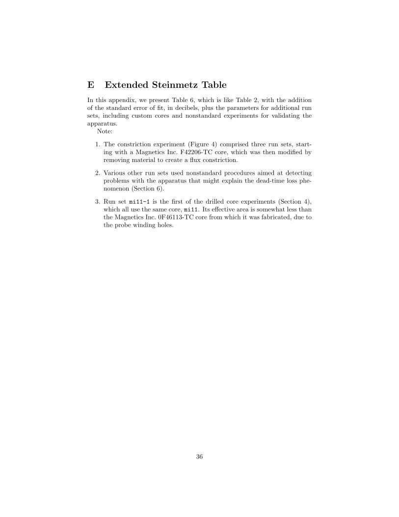
E Extended Steinmetz Table

In this appendix, we present Table 6, which is like Table 2, with the additionof the standard error of fit, in decibels, plus the parameters for additional runsets, including custom cores and nonstandard experiments for validating theapparatus.

Note:

1. The constriction experiment (Figure 4) comprised three run sets, start-ing with a Magnetics Inc. F42206-TC core, which was then modified byremoving material to create a flux constriction.

2. Various other run sets used nonstandard procedures aimed at detectingproblems with the apparatus that might explain the dead-time loss phe-nomenon (Section 6).

3. Run set mi11-1 is the first of the drilled core experiments (Section 4),which all use the same core, mi11. Its effective area is somewhat less thanthe Magnetics Inc. 0F46113-TC core from which it was fabricated, due tothe probe winding holes.

36

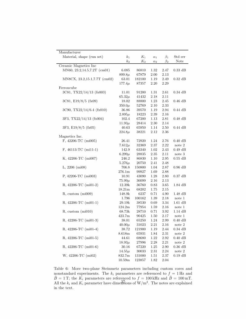
ManufacturerMaterial, shape (run set) k1 K1 α1 β1 Std err

k2 K2 α2 β2 Note

Ceramic Magnetics IncMN60, 23.2,14.5,7.2T (cm01) 6.085 86810 1.32 2.47 0.33 dB

899.8µ 67879 2.00 2.13MN8CX, 23.2,15.1,7.7T (cm02) 63.01 182100 1.19 2.49 0.32 dB

177.4µ 87357 2.20 2.29Ferroxcube

3C81, TX22/14/13 (fx003) 11.01 91200 1.31 2.61 0.34 dB65.32µ 41432 2.18 2.11

3C81, E19/8/5 (fx09) 18.02 88800 1.23 2.45 0.46 dB350.0µ 52769 2.10 2.33

3C90, TX22/14/6.4 (fx010) 36.86 39570 1.19 2.94 0.44 dB2.895µ 18223 2.39 2.16

3F3, TX22/14/13 (fx004) 102.4 67200 1.13 2.81 0.48 dB11.93µ 28414 2.30 2.14

3F3, E19/8/5 (fx05) 40.63 65950 1.14 2.50 0.44 dB224.8µ 38221 2.12 2.36

Magnetics Inc.F, 42206-TC (mi005) 26.41 72920 1.24 2.76 0.40 dB

7.612µ 32369 2.37 2.22 note 2F, 46113-TC (mi11-1) 142.9 63340 1.02 2.43 0.49 dB

6.299µ 28835 2.35 2.11 note 3K, 42206-TC (mi007) 246.2 86830 1.10 2.95 0.55 dB

5.276µ 20750 2.41 2.48L, 2206 (mi08) 706.8 150800 1.04 2.87 0.96 dB

276.1m 99927 1.69 2.88P, 42206-TC (mi003) 10.91 43090 1.28 2.80 0.37 dB

75.99µ 36099 2.16 2.13R, 42206-TC (mi01-2) 12.39k 36760 0.83 3.65 1.84 dB

18.21m 68202 1.75 2.15R, custom (mi009) 148.9k 6237 0.71 4.90 1.48 dB

1.796 100162 1.39 2.18 note 1R, 42206-TC (mi01-1) 29.19k 38530 0.69 3.34 1.61 dB

124.2m 77954 1.59 2.16 note 1R, custom (mi010) 68.73k 28710 0.71 3.92 1.14 dB

423.7m 90425 1.50 2.17 note 1R, 42206-TC (mi01-3) 38.01 65250 1.24 2.99 0.40 dB

40.00µ 31023 2.21 2.16 note 2R, 42206-TC (mi01-4) 38.72 121900 1.19 2.44 0.34 dB

8.618m 65931 1.84 2.31 note 2R, 42206-TC (mi01-5) 44.61 68680 1.22 2.92 0.40 dB

18.93µ 27996 2.28 2.21 note 2R, 42206-TC (mi01-6) 30.16 67220 1.25 2.90 0.36 dB

14.55µ 30033 2.31 2.24 note 2W, 42206-TC (mi02) 832.7m 131000 1.51 2.37 0.19 dB

10.59m 123857 1.82 2.04

Table 6: More two-plane Steinmetz parameters including custom cores andnonstandard experiments. The ki parameters are referenced to f = 1Hz andB = 1T; the Ki parameters are referenced to f = 100 kHz and B = 100mT.All the ki and Ki parameter have dimensions of W/m2. The notes are explainedin the text.

37

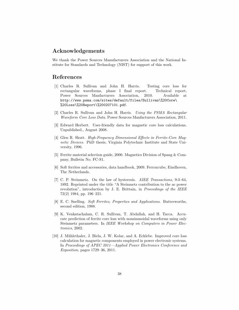
Acknowledgements

We thank the Power Sources Manufacturers Association and the National In-stitute for Standards and Technology (NIST) for support of this work.

References

[1] Charles R. Sullivan and John H. Harris. Testing core loss forrectangular waveforms, phase I final report. Technical report,Power Sources Manfacturers Association, 2010. Available athttp://www.psma.com/sites/default/files/Sullivan\%20Core\

%20Loss\%20Report\%200207101.pdf.

[2] Charles R. Sullivan and John H. Harris. Using the PSMA RectangularWaveform Core Loss Data. Power Sources Manfacturers Association, 2011.

[3] Edward Herbert. User-friendly data for magnetic core loss calculations.Unpublished., August 2008.

[4] Glen R. Skutt. High-Frequency Dimensional Effects in Ferrite-Core Mag-netic Devices. PhD thesis, Virginia Polytechnic Institute and State Uni-versity, 1996.

[5] Ferrite material selection guide, 2000. Magnetics Division of Spang & Com-pany, Bulletin No. FC-S1.

[6] Soft ferrites and accessories, data handbook, 2009. Ferroxcube, Eindhoven,The Netherlands.

[7] C. P. Steinmetz. On the law of hysteresis. AIEE Transactions, 9:3–64,1892. Reprinted under the title “A Steinmetz contribution to the ac powerrevolution”, introduction by J. E. Brittain, in Proceedings of the IEEE72(2) 1984, pp. 196–221.

[8] E. C. Snelling. Soft Ferrites, Properties and Applications. Butterworths,second edition, 1988.

[9] K. Venkatachalam, C. R. Sullivan, T. Abdallah, and H. Tacca. Accu-rate prediction of ferrite core loss with nonsinusoidal waveforms using onlySteinmetz parameters. In IEEE Workshop on Computers in Power Elec-tronics, 2002.

[10] J. Muhlethaler, J. Biela, J. W. Kolar, and A. Ecklebe. Improved core losscalculation for magnetic components employed in power electronic systems.In Proceedings of APEC 2011—Applied Power Electronics Conference andExposition, pages 1729–36, 2011.

38

Testing Core Loss for Rectangular Waveforms

February 7, 2010

Charles R. Sullivan

John H. Harris Thayer School of Engineering at Dartmouth

charles.r.sullivan@dartmouth.edu http://engineering.dartmouth.edu/inductor

8000 Cummings Hall Hanover, NH 03755, USA

Edward Herbert

closs@eherbert.com http://fmtt.com/

1 Dyer Cemetery Road Canton, CT 06019, USA

Sponsored by

The Power Sources Manufacturers Association email: power@psma.com

http://www.psma.com/ P.O. Box 418

Mendham, NJ 07945-0418 Tel: (973) 543-9660 Fax: (973) 543-6207

[11] Charles R. Sullivan, John H. Harris, and Edward Herbert. Core loss pre-dictions for general PWM waveforms from a simplified set of measureddata. In Applied Power Electronics Conference and Exposition (APEC),2010 25th Annual IEEE, pages 1048–1055, February 2010.

[12] Curve fit equations for ferrite materials, 1999. Magnetics Division of Spang& Company, Bulletin No. FC-S7.

[13] Jieli Li, T. Abdallah, and C. R. Sullivan. Improved calculation of coreloss with nonsinusoidal waveforms. In IEEE Industry Applications SocietyAnnual Meeting, pages 2203–2210, 2001.

39

115

Appendix B–The Data In general, the data is provided both as zip files, for convenient download and as expanded files, for convenient browsing.

Using the data

For those who are familiar with SQLite, the database files may be useful (Phase II Project only). There is a good extension to the Firefox browser that I used to view the files. The coreloss.db file contains all of the data from the run sets .csv files, plus a number of calculated values determined using MatLab.

I preferred using the .csv files, partly because it is necessary for the Pilot Project data but mostly because I wanted to process the data to export to SPICE, and it is necessary to convert the negative times. It is easy to do that and to do other calculations in spreadsheets. See Appendix C, The Excel Tool–Viewing the Data

In addition to the data provided by Dartmouth, I have converted some of the data into Excel files. In addition, I have resorted some of the data in Excel files. These add nothing new, but may be convenient to the user and ar available for download at http://www.psma.com/coreloss/tools

The added files are summarized at the end of this Appendix.

Pilot Project Data

The data for the Pilot Project can be downloaded at http://www.psma.com/coreloss/pilot

The are three sub-directories,

1. Characterization-data

2. Ferrite-data

3. Powdered-iron-data

Characterization-data sub-directory

The characterization data summarizes the square-wave results from the various tests, with headers of Frequency, Peak flux linkage, Volts/turn, Average loss and Loss per cycle.

The characterization data is provided in several formats: MicroSoft Excel (.xls), Comma-separated value (.csv), plain text (.dat). There are shortcuts to MicroSoft Access files, but there seem to be no corresponding files. The report says that there are Matlab (.mat) files, but they seem to be missing.

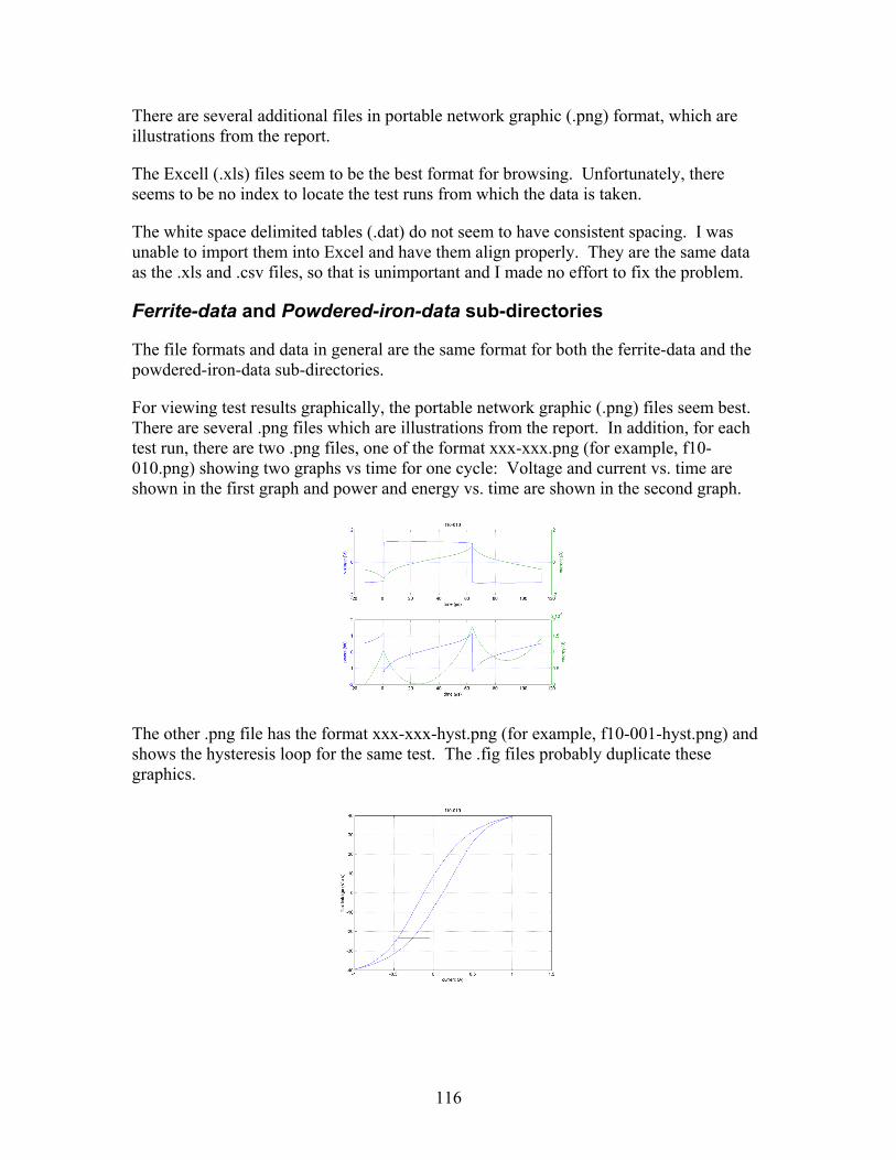
116

There are several additional files in portable network graphic (.png) format, which are illustrations from the report.

The Excell (.xls) files seem to be the best format for browsing. Unfortunately, there seems to be no index to locate the test runs from which the data is taken.

The white space delimited tables (.dat) do not seem to have consistent spacing. I was unable to import them into Excel and have them align properly. They are the same data as the .xls and .csv files, so that is unimportant and I made no effort to fix the problem.

Ferrite-data and Powdered-iron-data sub-directories

The file formats and data in general are the same format for both the ferrite-data and the powdered-iron-data sub-directories.

For viewing test results graphically, the portable network graphic (.png) files seem best. There are several .png files which are illustrations from the report. In addition, for each test run, there are two .png files, one of the format xxx-xxx.png (for example, f10-010.png) showing two graphs vs time for one cycle: Voltage and current vs. time are shown in the first graph and power and energy vs. time are shown in the second graph.

The other .png file has the format xxx-xxx-hyst.png (for example, f10-001-hyst.png) and shows the hysteresis loop for the same test. The .fig files probably duplicate these graphics.

117

Outfile.dat has an index of the test runs. I cannot identify the data in outfile.csv; it is not the same.

In the powdered-iron-data directory, there are additional indexes of the runs with self-explanatory names: i02-all-runs.dat and i02-good-runs.dat.

For accessing the raw data, the comma-separated-value (.csv) files are used. The formats for the Pilot Project data and the Phase II data is similar, and they are described below.

There are several miscellaneous files that I did not explore. Some seem to be duplicate graphics in other formats. Some seem to be used by the test equipment.

118

Phase II Project Data

The data for the Phase II Project can be downloaded at http://www.psma.com/coreloss/phase2

There is an exhaustive description of using the data in the Users Manual (user.pdf), and those who want to make maximum use of the data should refer to that manual. Following is a summary:

• cores/ directory. The cores/ directory contain files with data, other than the experimental results, such as manufacturer's specifications, describing the magnetic cores under test.

• sets/ directory. The sets/ directory contains various subdirectories, each containing the data for one run set, including data files describing the run set, and subdirectories with raw data and plots. A run set subdirectory has the run set identifier for its name, and typically contains about 50 MB of data, for several hundred runs, each characterized by frequency, peak voltage, and wave shape.

The contents of the sets/ directory are described in more detail below.

• zips/ directory. The zips/ directory contains zip archive files of the run set directories, for convenient downloading and distribution. The zip files have names like runs-setId.zip. Each zip file is self-contained, containing supporting information for the user. There is also an archive, cores.zip, of the contents of the /cores/ directory.

• steinmetz.dat is a table of two-plane, square-wave Steinmetz parameters for the various materials tested in the project.

• setsrept.txt is a summary of run set parameters to help in locating run set directories of interest.

• corerept.txt contains a summary of the information contained in the cores/ directory data files.

• corerept.csv is a comma-separated-value text file table of parameter for the various cores tested in the project. Like corerept.dat it summarizes the information contained in the cores/ directory, but in a machine-readable format.

119

• coreloss.db is an SQLite database file. The information it contains duplicates that found in the other files of the data set, and is only provided for the convenience of experienced SQLite users.

• readme.txt is the readme file for this directory. It is for the benefit of someone browsing the directory, and mostly directs the user to the user manual.

(The .txt and .dat files can be viewed with an ordinary ASCII text editor such as Notepad or Wordpad.)

The sets/ directory

The sets/ directory contains 30 sub-directories, each containing files associated with a set of tests. Most are for individual cores, but some represent multiple sets on one core or core type, identified by a common prefix. As an example, set fx003 are tests on one core, Ferroxcube, TX22/14/13 shape, 3C81 material. The sets mi01-1 through mi01-6 are tests run on three cores Magnetics Inc., 42206-TC shape, R material. The sets mi11-1 through mi11-8 are sets run on the drilled core, with various different test windings. See setsreport.txt in the main directory for a description of each set.

Readme.txt file of sets/ directory:

The readme.txt file contains a comprehensive explanation of the files in the sets/ sub-directories and is copied here, with edits. [Read-me File for PSMA Core Loss Run-set Directories. readme.txt (from Coreloss rev 212)] This directory contains data generated by the PSMA Coreloss testing system. In this generic readme file, we use <setId> to refer to the run-set identifier of this particular run set. See the gen-<setId>.dat file for the details of this run set. See user.pdf for a detailed explanation of the data. The following files (and perhaps others) are contained in this directory: user.pdf: This is the user's manual for the PSMA Core Loss data set. gen-<setId>.dat: This file is the input to the run-set generator program and also contains additional information in the note and comment fields. runs-<setId>.dat: This is the output file created by the run set generator. It is the input file for the coreloss test apparatus. data-<setId>.dat: This file is generated by the Matlab code and is quite similar to the runs-<setId>.dat file, but with

120

additional computed fields on the right, including energy per period, and power. core-<coreId>.dat The core data for the core used in the run set. A core ID uniquely identifies a manufacturer and part number, but does not distinguish between different instances of the manufacturer's SKU. This file is a copy of the core data file mentioned in the gen-<setId>.dat file, made at the time the directory was zipped. readme.txt: This file. <setId.db: This is a SQLite relational database file containing all the scope data. It can be joined with the main database file, coreloss.db, found in the data/ directory. The data differ from that in the scope/*.csv files in that DC offsets have been removed, and a volt-seconds column has been added. See the user manual user.pdf for more details. Note: The times start with negative values, a problem for some uses of the data. scope-ddl.sql: This is the SQL data description for the SQLite database file, <setId>.db, above.

These subdirectories contain the experimental data and results: scope/: This directory contains the output files written by the oscilloscope during the coreloss run set. The CSV files are the raw data. The text files give the oscilloscope configuration.

For using the data, the comma-separated-value (.csv) files are used. The formats for the Pilot Project data and the Phase II data is similar, and they are described below. Note: The times start with negative values, a problem for some uses of the data. Also, the voltage and current data have zero offsets that must be removed. images/: This directory contains waveform plot images generated by the Matlab code from the files in the scope/ directory. There are three formats. Each image has four plots: Voltage vs time, current vs. time, power vs time, and energy vs. time, all for one particular waveform. results/: This directory contains images of various plots comparing the core loss for similar pulse shapes in different waveform contexts.

121

auximages/: The embedded probe winding experiments have an additional image directory.

Added files

I have added several file for the convenience of the user. These can be downloaded at http://www.psma.com/coreloss/tools

The following is a pdf, an edited copy of "setsrept.txt." The physical and magnetic sized of the cores have been added where known.

modsetsrept.pdf

The following are the Excel Tool. The first is written in Office 2003 Excel and is the one that I use. The second is converted to Office 2007 and is untested.

extool.xls, 1.8 M

extoolm.xlsm 1 M

The following is the Pilot Project ferrite data outfile.dat, converted ot .xls.

outfile.xls 121 k

The following files are the data table from coreloss.db, opened in FirefoxSQLite, exported as .csv with headers added. The second was that file, opened in Excel 2003, saved as an .xls file.

data.csv 663 k

data.xls 1.45 M

The files following are derived from data.xls. They have been sorted and some rows and columns deleted. The names are descriptive.

purged_data.xls 636 k

drilled_data.xls 367 k

purged_expand_data.xls 250 k

purged_hippo_data.xls 251 k

purged_sqare_data.xls 211 k

122

Appendix C The Excel Tool–Viewing the Data To make it easier to use the data, I created an Excel Tool. It is generated using Excel in MSOffice 2003, and uses VBA macros. Excel macros are notoriously buggy, particularly if used in different versions of Excel or on different computers with different operating systems. The Excel Tool was written as an aid in writing this report. It is a bonus if others can use it. It can be downloaded at http://www.psma.com/coreloss/tools/extool.xls

Using the data

For those who are familiar with SQLite, the database files may be useful (Phase II Project only). There is a good extension for the Firefox browser that I used to view the files. The coreloss.db file contains all of the data from the run sets .csv files, plus a number of calculated values determined using MatLab.

I preferred using the .csv files, partly because it is necessary for the Pilot Project data regardless, but mostly because I wanted to process the data to export to SPICE, and it is necessary to convert the negative times. It is easy to do that and to do other calculations in spreadsheets.

Source data files, .csv data

The comma-separated-value (.csv) files are the same format for the Pilot Project and the Phase II Project. They are easily imported into MicroSoft Excel spreadsheets.

The first two lines are headers: x-axis SYNC OUT V I second Volt Volt Volt Ampere

The first column A "x-axis/second" is the time, in seconds. Unfortunately, the time starts with a negative value, which cannot be used by some programs, like SPICE. Time = 0 is a trigger event.

The second column B "SYNC/Volt" is a signal from the waveform generator. Detecting rise and fall times may be useful for synchronizing data from other test runs.

The third column D "OUT/Volt" is another output of the waveform generator for most test runs, but it is used for the sense winding voltage for the drilled core tests.

The fourth column E "V/Volt" is the voltage of the voltage sense winding. This data may have a voltage offset that must be removed if the data is used for calculations.

The fifth column F "I/Ampere" is the current probe. This data may have a current offset that must be removed if the data is used for calculations.

123

In general, I found that the last row of data is unreliable, so I did not use it for further calculations nor did I export it to SPICE.

Using The Excel Tool

There are four functions of the Excel Tool for handling data:

1. Import the data from the selected source file.

2. Calculate needed parameters

3. Export the data as files that can be used by SPICE and other programs

4. Display selected calculated data as graphs and parameters.

The Excel Tool can be downloaded from http://www.psma.com/coreloss/tools/extool.xls

The Cmd! sheet of the Excel Tool workbook is shown on the next page. Various parts of the worksheet, and how to use them, are explained in the text following.

Macros

The Excel Tool uses macros. Macros can contain viruses, so many company servers block macros, and the settings on personal computers may have to be changed to run the macros. I suggest not running macros using any files that have been obtained from a third party. The user should download the Excel Tool himself self from the web site indicated above, to ensure that the macros have not been compromised.

Import and Export tool

The first sheet of the Excel workbook (Cmd!) is for control and display. An input file from the Pilot Project or the Phase II Project is selected.

Click the top right button to select the input file, and confirm it by clicking the dialog box. Next, the processing is initiated by clicking the bottom right button, which imports the data, executes a number of calculations, exports the calculated data and displays the results as graphs and parameters.

124

Excel Tool

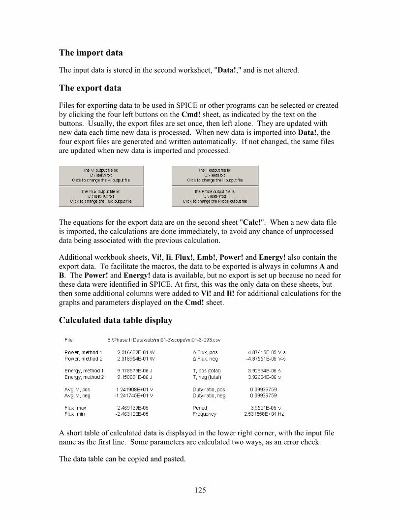
125

The import data

The input data is stored in the second worksheet, "Data!," and is not altered.

The export data

Files for exporting data to be used in SPICE or other programs can be selected or created by clicking the four left buttons on the Cmd! sheet, as indicated by the text on the buttons. Usually, the export files are set once, then left alone. They are updated with new data each time new data is processed. When new data is imported into Data!, the four export files are generated and written automatically. If not changed, the same files are updated when new data is imported and processed.

The equations for the export data are on the second sheet "Calc!". When a new data file is imported, the calculations are done immediately, to avoid any chance of unprocessed data being associated with the previous calculation.

Additional workbook sheets, Vi!, Ii, Flux!, Emb!, Power! and Energy! also contain the export data. To facilitate the macros, the data to be exported is always in columns A and B. The Power! and Energy! data is available, but no export is set up because no need for these data were identified in SPICE. At first, this was the only data on these sheets, but then some additional columns were added to Vi! and Ii! for additional calculations for the graphs and parameters displayed on the Cmd! sheet.

Calculated data table display

A short table of calculated data is displayed in the lower right corner, with the input file name as the first line. Some parameters are calculated two ways, as an error check.

The data table can be copied and pasted.

126

Graphs

Six graphs are displayed on the left side of the Cmd! worksheet. These are generated using the Excel Chart function, but use the same data as is generated for export.

The hysteresis loop uses the Flux and the input current Ii as its axes, so it displays Volt-seconds vs Amperes. This is a device hysteresis loop, so it is not corrected for turns, nor does it have any dimensional factors.

These graphs can be copied and pasted into Word, but I was unable to paste them directly into email. Once copied into Word, they can then be copied and pasted to email.

The power and energy data are generated but not exported. The files are available for manual export, or the macro could be edited to add export files for them.

The graphs can be copied and pasted into MSWord. I was unable to paste them into email, but if copied to MSWord first, the MSWord copy can then be copied and pasted into email.

Hidden data on the Cmd! worksheet

Underlying the buttons and graphs are a number of columns of data from the other worksheets. These data are not visible because they are covered by the other features and because the text color is white. This was done so that the export data were on the same worksheet as the buttons that controlled the export files. This would be done differently if done over, but it is not worth the effort to change it.

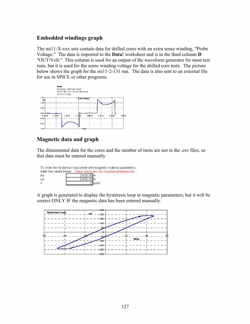
127

Embedded windings graph

The mi11-X-xxx sets contain data for drilled cores with an extra sense winding, "Probe Voltage." The data is imported to the Data! worksheet and is in the third column D "OUT/Volt." This column is used for an output of the waveform generator for most test runs, but it is used for the sense winding voltage for the drilled core tests. The picture below shows the graph for the mi11-2-131 run. The data is also sent to an external file for use in SPICE or other programs.

Magnetic data and graph

The dimensional data for the cores and the number of turns are not in the .csv files, so that data must be entered manually

A graph is generated to display the hysteresis loop in magnetic parameters, but it will be correct ONLY IF the magnetic data has been entered manually.

128

Data files on the Calc! sheet:

Note: The data in the last row of the imported files seems to be unreliable, so it is not used. The input data has 1000 rows, and the calculated data has 999 rows.

Calc A: "Time, all positive". SPICE cannot use negative times, and the imported data starts at a negative time, with 0 being a "trigger point." This is the time from Data!A modified so that it starts at 0.

Calc C: "Out, offset removed". This is the voltage of column Data!C with the offset removed. This data is not used except for the drilled core tests in Phase II.: "V, offset removed". This is the voltage of column D with the offset removed.

Calc D: "V, offset removed". This is the voltage of column Data!D with the offset removed.

Calc E: "I, offset removed" This is the current of column Data!E with the offset removed.

Calc F:: "Flux cumulative". This is the cumulative flux from time = 0 (column Calc!A, the sum of the product of the voltage in column Calc!D and the incremental time. Effectively, it is a piece-wise integration of the voltage ∫ v dt.

Calc G: "Flux, offset removed". This is the flux of column Calc!F with the offset removed.

Calc H: "Power". This is the instantaneous power, the product of the voltage in column Calc!D and the current in column Calc!E.

Calc I: "Energy". This is the cummulative sum of the product of the power of column Calc!H and the incremental time. Effectively, it is a piece-wise integration of the power ∫ p dt.

Calc B: "Time, new zero". This function allows the user to select a different point as time 0. I do not use this data, and if it is used, additional processing is needed to sort on this column or to discard rows having negative time. This is the time of column Data!A with 0 pinned to a trigger time of the user's choice. Before sorting, the chosen time becomes 0 in column Calc!B, and in rows following, the time increments from 0. Earlier times increment from the last value in column.

If this function is used, and after calculation, if the data is sorted on this column, time increments from 0 and all data points follow in order so that a graph can be made using the chosen trigger time as the origin. Again, I did not identify any need for this function, and no export is done for these data.

129

Data on the Vi!, Ii!, Flux!, Emb!, Power! and Energy! worksheets

There are six additional worksheets, Vi!, Ii!, Flux!, Emb!, Power! and Energy!.

Mostly, this is data rearranged in convenient columns for export, with the headings removed. To be used in SPICE as PWL inputs, the data must be in two columns, time and the parameter being simulated. (It is supposed to be possible to add comment lines in the PWL data with a leading apostrophe so that the line is ignored, but instead it generated errors, so the headers were removed.)

Equations for the export data:

Removing the negative times

To convert the time column so that the time is always positive, add a new column Calc A. For each cell, starting with Calc!A3, I subtracted the value of the first time data cell Data!$A$3 from the times in column Data!A using the expression =Data!$A3-Data!$A$3. When extended down the column, the subsequent cells become =Data!$A4-Data!$A$3, =Data!$A5-Data!$A$3, etc., for example Calc!A3: =Data!$A3-Data!$A$3 Calc!A4: =Data!$A4-Data!$A$3 Calc!A5: =Data!$A5-Data!$A$3

Etc.

Removing the zero offset voltages and current.

Use new columns Calc!C, Calc!D and Calc!E. In the second cell of the new columns, insert the average value of the respective voltages or current for columns Data!C, Data!D or Data!E. For example, to remove the off set from the output current in column Data!E, and put the result in the new column Calc!E, calculate the average of column Data!E and put it in Calc!E2: =AVERAGE(Data$E3:$E1002). Then subtract this value from each cell in column E, for example:

Calc!E2: =AVERAGE(Data!$E:Data!$E1002)

Calc!E3: =Data!$E3-$E$2.

Calc!E4: =Data!$E4-$J$2.

Etc.

Calculating the flux

To display a hysteresis loop, the flux is needed for the Y-axis. From the data, it is not possible to know the true value of the flux but the incremental flux is calculated as the product of the voltage in column Calc!D and the incremental time, and that is summed to

130

get the cumulative flux from time = 0, with reference to column Calc!A. Add a new column Calc!F. Calc!F3: =($A4-$A3)*$D3 Calc!F4: =$F3+($A4-$A3)*$D3 Calc!F5: =$F4+($A5-$A4)*$D4

etc.

The offset is then removed in the same manner as it is for the voltages and current with the result put in column Calc!G. Calc!G2: =AVERAGE($F4:$F1002) Calc!G3: =$F3-$FG2 Calc!G4: =$F4-$FG2

etc.

Calculating the power and energy

Power and energy are more easily calculated in SPICE, but if desired, they can be calculated in the worksheet. Use column Calc!H for the power and column Calc!I for the energy.

Power is the product of the voltage in column Calc!D and the current in column Calc!E, for example: Calc!H3: =$D3*$E3 Calc!H4: =$D4*$E4 Calc!H5: =$D5*$E5

Etc.

The energy input during one cycle is the cumulative sum of the product of the power in column Calc!H and the incremental time from column Calc!A, for example: Calc!I3: =($A4-$A3)*$H3 Calc!I4: =$I3+($A4-$A3)*$H3 Calc!I5: =$I4+($A5-$A4)*$H4

Etc.

Changing the zero time reference (Alternative)

To use an event as the zero time reference point, further convert the time data using a new column Calc!B. Find the time in column Calc!A that corresponds to the desired zero reference, and put that value in Cald!B2. Subtract that value from each cell in column Calc!A, for example, $A3-$B$2. If the result is negative, then add the difference between the final value in column Data!A, for example, (Data!$A$1001) to the next cell in column F. For example, to set the new 0 at time = 1.26880000E-05, put that value in Calc!B2. Alternatively, put in a cell containing that value, for example Calc!A613. For example:

131

Calc!B2: 1.26880000E-04 Or:

Alternatively, Calc!B2: =$A$613 Calc!B3: =IF((Data!$A3-$B$2)<0, Data!$A4+Data!$A$1001-$B$2, $A3-$B$2)) Calc!B4: =IF((Data!$A4-$B$2)<0, Data!$A5+Data!$A$1001-$B$2, $A4-$B$2)) Calc!B5: =IF((Data!$A5-$B$2)<0, Data!$A6+Data!$A$1001-$B$2, $A5-$B$2))) Etc. Then sort the data ascending, using column Calc!B.

Miscellaneous equations on other worksheets

On the Vi! worksheet, four additional columns are generated.

In column G, the voltage in column B is tested to see if it is above a threshold equal to 1/3 of the maximum voltage in column B. If it is, the time increment is put in the cell, otherwise 0. The sum is the total time that the voltage is positive (above the threshold), and that is displayed the positive time (T-pos) on the Cmd! sheet.

In column H, the voltage in column B is tested to see if it is below a threshold equal to 1/3 of the minimum voltage in column B. If it is, the time increment is put in the cell, otherwise 0. The sum is the total time that the voltage is negative (below the threshold), and that is displayed as the negative time (T-neg) on the Cmd! sheet.

In column J, the data in column B (the input voltage) is multiplied by the data in column G to generate the incremental positive flux. The sum is displayed as the ∆ positive flux on the CMD! sheet.

In column K, the data in column B (the input voltage) is multiplied by the data in column H to generate the incremental negative flux. The sum is displayed as the ∆ negative flux on the CMD! sheet.

On the Ii! worksheet, there are three extra columns. (Columns A and B are the data for the Ii export file).

Column C contains the flux, so that columns B and C are the data source to generate the hysteresis graph on the CMD! sheet.

Columns E and F are the data in columns B and C, factored by the magnetic parameters (core area, core length, turns) as the source data to generate the hysteresis loop in magnetic parameters on the Cmd! sheet.

132

Miscellaneous calculations on the Cmd! worksheet

The following calculate parameters of the data table on the Cmd! worksheet.

Power, method 1 is calculated as =AVERAGE(Power!B1:B999).

Power, method 2 is calculated as =Energy!B999/Energy!A999. Energy!B999 is the final value of the energy column B on the worksheet Energy!. Energy!A999 is the period.

Energy, method 1 is =Energy!B999, the final value of the energy column B on the worksheet Energy!.

Energy, method 2 is calculated as =AVERAGE(Q42,Q43)*Calc!A999, where Q42 is the power, method 1, Q43 is Power, method 2 and Calc!A999 is the period.

The following six calculations are based upon calculations on the worksheets Vi! and Flux! as explained above.

∆ Flux, Pos is calculated as =SUM(Vi!J1:J999).

∆ Flux, Neg is calculated as =SUM(Vi!K1:K999).

T Pos (total) is calculated as =SUM(Vi!K1:K999)

T Neg (total) is calculated as =SUM(Vi!$H1:$H999)

Flux, max is calculated as =MAX(Flux!B1:B999).

Flux, min is calculated as =MIN(Flux!B1:B999)

Calc!A999 contains the last time of data, with negative values of time converted.

Period is =Calc!A999.

Frequency is calculated as =1/Calc!A999.

Exporting voltages, current and flux into SPICE

SPICE voltage and current sources include a Piecewise Linear Source (PWL) function. Starting at time = 0, a voltage or current is specified, then a table is built, line by line, each line specifying a new time and a new voltage or current. In this manner, any arbitrary waveform can be constructed.

With 999 points, the calculated data cannot be entered by typing each line, but the calculated data is formatted correctly so that it can be entered manually by "copy and paste" or by automatic file export.

133

Manual export:

Data can be imported into SPICE using the PWL function of a voltage or current source. In the PWL function, the first column is time, and the second column is the parameter list.

To import the data manually, a column with the time and a column with parameters are selected, copied and pasted into the PWL function. For example, to import the output voltage Vi, select column Calc!A, the time, then pressing <Ctrl> select column Calc!D, the voltage. These columns then can be copied and pasted into the PWL function of the voltage source.

This is repeated for the current and flux. It can also be used for the power and energy, but since the time, voltage and current are available to SPICE once imported, power and energy can be generated in SPICE, saving the effort of two copy and paste steps.

This is explained in more detail with examples in Appendix D.

Automated file export:

When new data is imported into Data!, four files are generated and written automatically. These files are selected or created on the Cmd! sheet. The export file paths and names can be chosen once, then left alone. In this case, the same files are updated when new data is imported and processed.

One of the choices for importing PWL data into SPICE is "File." A text file is designated, and each time the SPICE model is run, the PWL data is read from that file. If the file is updated before the run, the new data is used.

In this way, once a new source file is imported into the spreadsheet, the data is also exported to the SPICE file and is immediately available for use.

134

Appendix D-The SPICE Tool–Using SPICE to examine data These directions show how I went through the steps. The Excel Tool is available at http://www.psma.com/coreloss/tools/extool.xls It is written in Excel from MSOffice 2003 on a Win7 Home Premium operating system. Excel is notoriously quirky if used in different versions of MSOffice, on different operating systems or on different computers. If it works for you, that is a bonus.

I use IntuSoft ICAP/4 Windows as my SPICE program. It has not been updated for several years, and I have never successfully exported a SPICE model for others to run, so I won't even try. I have included the steps in making a SPICE circuit for viewing the data, so the reader can reconstruct a similar model in his own flavor of SPICE.

Macros

The Excel Tool uses macros. Macros can contain viruses, so many company servers block macros, and you may have to change the settings on personal computers to run the macros. I suggest not running macros using any files that have been given to you by others. Download the Excel Tool yourself from the web site indicated above, to ensure that they have not been hacked.

Import and process the data

Open the Excel Tool, select the core .csv file, and import the data. A number of calculations will be made, and selected results are displayed on the first page (Cmd!, sheet7). If you are using the automatically exported file, be sure to select their paths and names before processing.

Import selected data to SPICE

Open a model in SPICE, and create three voltage sources with grounds and terminals. I chose the terminal names "Vi", "Ii" and "Flux." The run set being viewed may be entered and displayed using a text box.

135

Open the voltage sources, each in turn, select Trans, then File and select the file to which the data has been saved. (Alternatively, open PWL and copy and paste the data from the Excel Tool, columns 1 and 2 of the Vi! worksheet, the Ii! worksheet and the Flux! worksheet.)

Once the file is selected, its wave shape is shown. Do the same for the current and flux files. Name and save the model file.

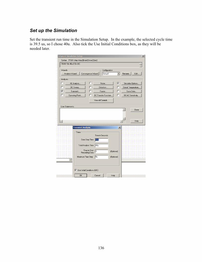
136

Set up the Simulation

Set the transient run time in the Simulation Setup. In the example, the selected cycle time is 39.5 us, so I chose 40u. Also tick the Use Initial Conditions box, as they will be needed later.

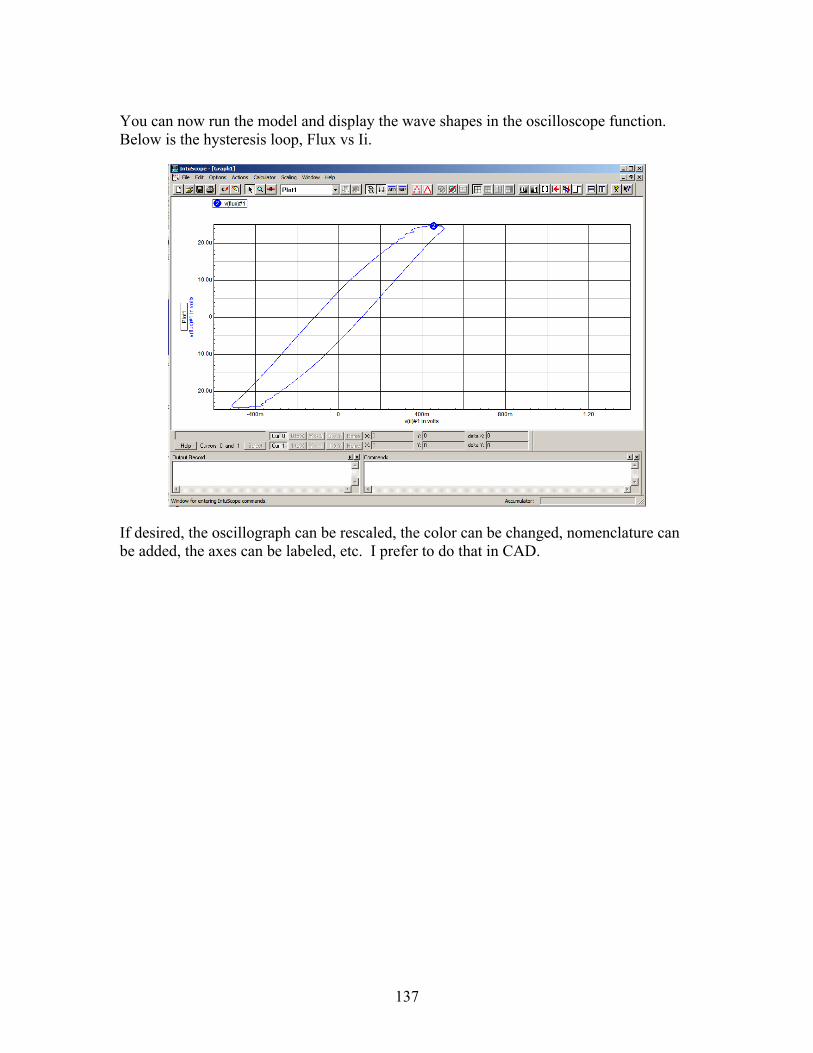
137

You can now run the model and display the wave shapes in the oscilloscope function. Below is the hysteresis loop, Flux vs Ii.

If desired, the oscillograph can be rescaled, the color can be changed, nomenclature can be added, the axes can be labeled, etc. I prefer to do that in CAD.

138

Appendix E The CAD Tool Export to CAD

The following examples use DesighCad 3D Max 18. I expect that the steps will work in other CAD programs, but I do not know.

To copy SPICE oscillograph to CAD (See Appendix D, The SPICE Tool), use the oscilloscope PRINT, then Copy to Clipboard. Open CAD and paste.

The first graph is "as imported". In the second graph, the legend has been added, extra grid has been deleted, the horizontal scale (but not the values) has been changed, the color has been changed and some artifacts have been cleaned up.

Print to graphics program

The CAD drawing may be copied and pasted into Word, maybe. Much better control of the appearance is possible "printing" the CAD drawing to a graphics program. I print to Adobe Acrobat, then crop the picture as desired and save it as a .tif file.

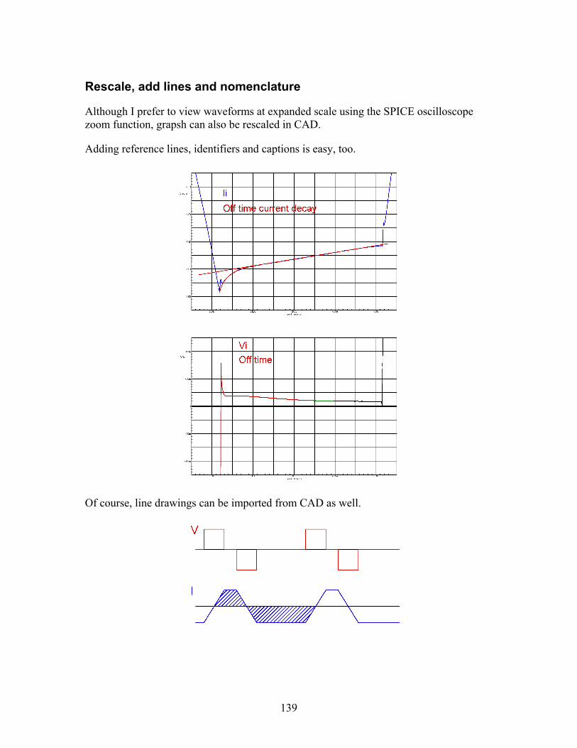
139

Rescale, add lines and nomenclature

Although I prefer to view waveforms at expanded scale using the SPICE oscilloscope zoom function, grapsh can also be rescaled in CAD.

Adding reference lines, identifiers and captions is easy, too.

Of course, line drawings can be imported from CAD as well.

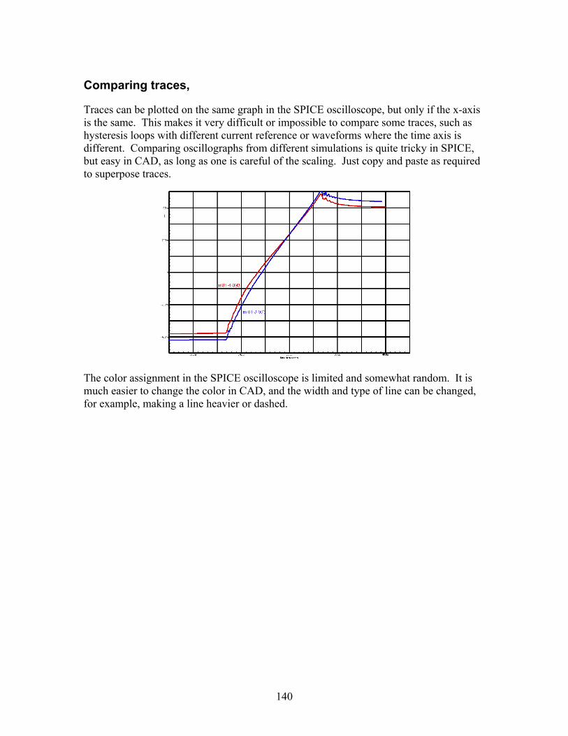
140

Comparing traces,

Traces can be plotted on the same graph in the SPICE oscilloscope, but only if the x-axis is the same. This makes it very difficult or impossible to compare some traces, such as hysteresis loops with different current reference or waveforms where the time axis is different. Comparing oscillographs from different simulations is quite tricky in SPICE, but easy in CAD, as long as one is careful of the scaling. Just copy and paste as required to superpose traces.

The color assignment in the SPICE oscilloscope is limited and somewhat random. It is much easier to change the color in CAD, and the width and type of line can be changed, for example, making a line heavier or dashed.

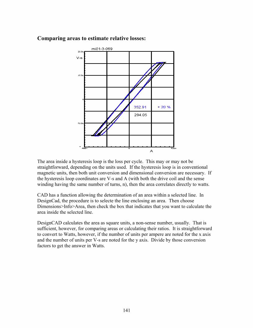
141

Comparing areas to estimate relative losses:

The area inside a hysteresis loop is the loss per cycle. This may or may not be straightforward, depending on the units used. If the hysteresis loop is in conventional magnetic units, then both unit conversion and dimensional conversion are necessary. If the hysteresis loop coordinates are V-s and A (with both the drive coil and the sense winding having the same number of turns, n), then the area correlates directly to watts.

CAD has a function allowing the determination of an area within a selected line. In DesignCad, the procedure is to selecte the line enclosing an area. Then choose Dimensions>Info>Area, then check the box that indicates that you want to calculate the area inside the selected line.

DesignCAD calculates the area as square units, a non-sense number, usually. That is sufficient, however, for comparing areas or calculating their ratios. It is straightforward to convert to Watts, however, if the number of units per ampere are noted for the x axis and the number of units per V-s are noted for the y axis. Divide by those conversion factors to get the answer in Watts.

142

Alternative graphics

While very useful, CAD is not the only way to import graphics.

Excel graphs can be copied, pasted, resized and rescaled. In Excel, select the drawing, then copy it. Paste it into Word. If it is the wrong size, select it, right click, and choose Format Picture. By default, size changes are proportional, but the height and width can be scaled differently.

Input Voltagei

-20.00

-15.00

-10.00

-5.00

0.00

5.00

10.00

15.00

0.0E+00 1.0E-06 2.0E-06 3.0E-06 4.0E-06 5.0E-06 6.0E-06 7.0E-06 8.0E-06 9.0E-06 1.0E-05

Time

Vi

Screenshots, made using the PrtSc key and opened (paste clipboard) in a photo program such as PhotoShop Elements. The figures can be cropped and saved as graphic files and imported.

This picture shows the SPICE oscilloscope, but the graph alone could be imported by cropping the PrtSc image to the graph only. This is faster but any editing has to be done in SPICE. The SPICE oscilloscope has some editing features, though I found them more cumbersome and limited.

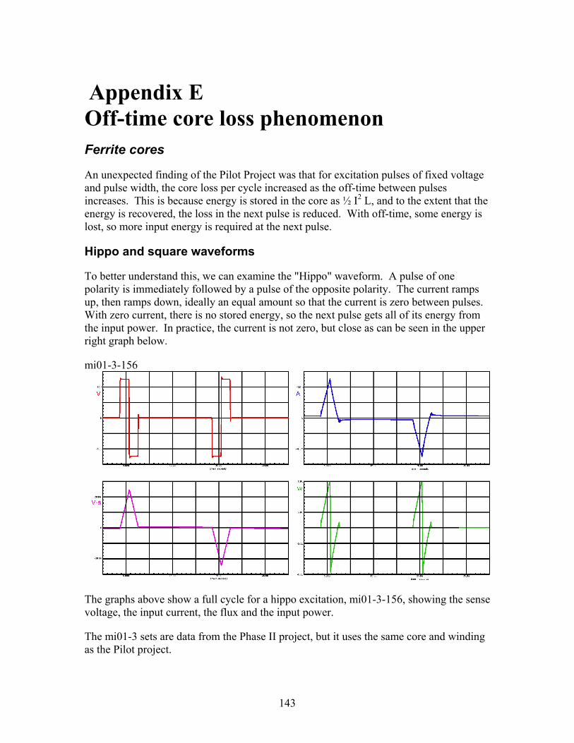
143

Appendix E Off-time core loss phenomenon Ferrite cores

An unexpected finding of the Pilot Project was that for excitation pulses of fixed voltage and pulse width, the core loss per cycle increased as the off-time between pulses increases. This is because energy is stored in the core as ½ I2 L, and to the extent that the energy is recovered, the loss in the next pulse is reduced. With off-time, some energy is lost, so more input energy is required at the next pulse.

Hippo and square waveforms

To better understand this, we can examine the "Hippo" waveform. A pulse of one polarity is immediately followed by a pulse of the opposite polarity. The current ramps up, then ramps down, ideally an equal amount so that the current is zero between pulses. With zero current, there is no stored energy, so the next pulse gets all of its energy from the input power. In practice, the current is not zero, but close as can be seen in the upper right graph below.

mi01-3-156

The graphs above show a full cycle for a hippo excitation, mi01-3-156, showing the sense voltage, the input current, the flux and the input power.

The mi01-3 sets are data from the Phase II project, but it uses the same core and winding as the Pilot project.

144

Following are graphs made using the SPICE scope function, zoomed in to the width of the excitation pulse, then copied and pasted into CAD.

Note that initially the input current is nearly zero, so there is no stored energy. After the positive voltage source, the current is maximum, and so is the stored energy. When the voltage goes negative, it takes nearly the entire pulse width for the current to reach zero, and during this time, the power is negative, that is, energy is returned to the voltage source. There is only a very short interval of positive power, right at the end.

Thus with the hippo excitation, we see an excitation pulse that requires the maximum power with no stored energy, followed by a pulse with maximum stored energy that

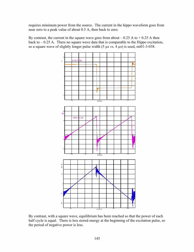
145

requires minimum power from the source. The current in the hippo waveform goes from near zero to a peak value of about 0.5 A, then back to zero.

By contrast, the current in the square wave goes from about – 0.25 A to + 0.25 A then back to – 0.25 A. There no square wave data that is comparable to the Hippo excitation, so a square wave of slightly longer pulse width (5 µs vs. 4 µs) is used, mi01-3-038.

By contrast, with a square wave, equilibrium has been reached so that the power of each half cycle is equal. There is less stored energy at the beginning of the excitation pulse, so the period of negative power is less.

146

Energy is the integral of power with respect to time,

∫= PdtE

The power curves can be copied and pasted into CAD, and the CAD area function can be used to find the area under the curves. Because the coordinates in CAD do not relate to Watts and time linearly, the area function does not derive Joules, but it can be converted to joules with appropriate scaling. In this example, we are using the area function for comparison only, so they need not be scaled. As long as the scale of the y and x axes are the same for the graphs being compared, the ratio is valid.

With an ideal inductor, all of the applied power would be stored as energy, and it would be returned during the reverse excitation pulse. In actuality, some of the applied power is stored as energy and some is dissipated. I do not know how to separate them, but qualitatively, 1415 units of energy went into the core, 828 units came back out, then 27 units more went in, for a net of 1415 -828 + 27 = 614 units for the cycle.

In the square wave excitation, equilibrium was established so that the power if each half cycle is equal. 382 units of power are returned, then 617 goes in, for a net of 617 – 382 = 235 units. That is for half a cycle, so 235 * 2 = 470 units for the cycle.

Even though the square wave cycle is significantly longer than the positive-negative pulses of the hippo waveform (5 µs vs. 4 µs), its net energy is less. The ratio is 470/614 = 0.765.

147

Expanded waveform

The graphs below show the excitation voltage, current, flux and the hysteresis loop for mi11-X-131 test runs. The graphs use component electrical engineering terms, volts, current and volt-seconds.

The current and voltage during the off time are shown below with expanded scale. As can be seen in the graphs on the previous page, the current ramp is quite small and the voltage is very low. The small voltage is positive and the current is negative, so that is power out of the core, but the amount of power is too small to account for the off time loss phenomena.

148

Two loss components are visible during the off-time. A short exponential reduction in current is followed by a long linear ramp. The latter is the very small IR drop of the circuit resistance and the circulating current. The initial exponential current drop probably accounts for most of the lost energy as a reduction of stored energy, E = ½ I2L. The red reference lines were added in CAD.

The flux changes revealed by the embedded windings do not appear to be a significant factor in explaining the off time loss phenomena. They are small, and the timing is not consistent.

Note the leading edge spike on the sense voltage winding.

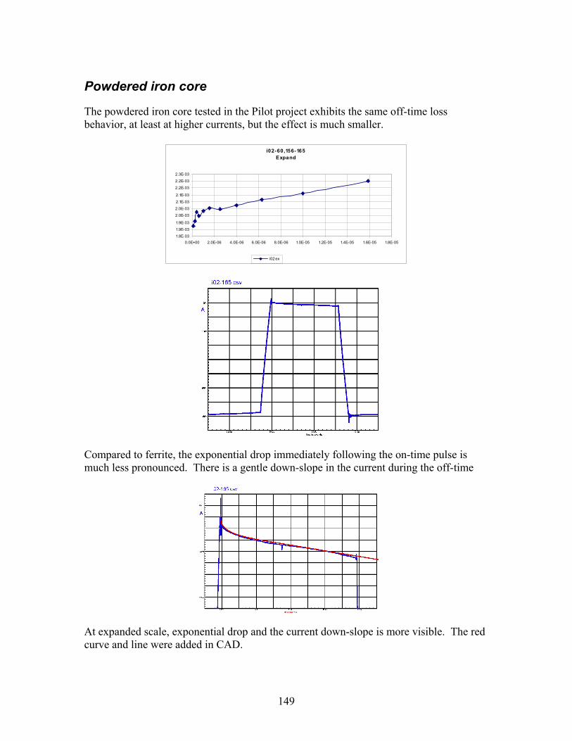
149

Powdered iron core

The powdered iron core tested in the Pilot project exhibits the same off-time loss behavior, at least at higher currents, but the effect is much smaller.

i02-60,156-165Expand

1.8E-03

1.9E-03

1.9E-03

2.0E-03

2.0E-03

2.1E-03

2.1E-03

2.2E-03

2.2E-03

2.3E-03

0.0E+00 2.0E-06 4.0E-06 6.0E-06 8.0E-06 1.0E-05 1.2E-05 1.4E-05 1.6E-05 1.8E-05

i02 ex

Compared to ferrite, the exponential drop immediately following the on-time pulse is much less pronounced. There is a gentle down-slope in the current during the off-time

At expanded scale, exponential drop and the current down-slope is more visible. The red curve and line were added in CAD.

150

Skew and symmetrical wave shapes

Skewed and symmetric wave shapes

A lot of data was taken with skewed and asymmetrical excitation. A blocking capacitor was used, and that makes these data difficult to interpret. The excitation of a magnetic core must have balanced volt-seconds, to avoid flux walking and saturation effects, and a blocking capacitor can ensure balanced excitation. Unfortunately, the blocking capacitor also forces balanced ampere-seconds (equal coulombs), and some wave shapes do not naturally have balanced currents.

The graph above shows a generic skewed excitation and the expected current for an ideal inductor. It is obvious by inspection that the ampere-seconds are not equal, so no skewed data was used for this report. It is not as obvious whether the ampere-seconds for an asymmetric waveform are not equal. Nonetheless, I regard asymmetric test data as suspect and did not use asymmetric data either.

The hysteresis loops for the skew data are distorted, the hysteresis loop below being an extreme example.

f10-133.csv

Hysteresis Loop

-2.0E-05

-1.0E-05

0.0E+00

1.0E-05

2.0E-05

3.0E-05

4.0E-05

5.0E-05

-4.0E-01 -2.0E-01 0.0E+00 2.0E-01 4.0E-01 6.0E-01 8.0E-01 1.0E+00 1.2E+00

A

V-s

A possible explanation is that the blocking capacitor forces the ampere-seconds (coulombs) to be equal. Because the current is positive for a much shorter time, its magnitude is forced to be much higher so that its average is zero. This can be seen both by the high positive currents in the hysteresis loop and in the current graph below.

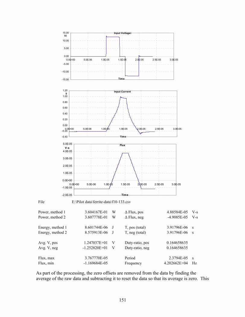
151

Input Voltagei

-15.00

-10.00

-5.00

0.00

5.00

10.00

15.00

0.0E+00 5.0E-06 1.0E-05 1.5E-05 2.0E-05 2.5E-05 3.0E-05

Time

Vi

Input Current

-0.40

-0.20

0.00

0.20

0.40

0.60

0.80

1.00

1.20

0.0E+00 5.0E-06 1.0E-05 1.5E-05 2.0E-05 2.5E-05 3.0E-05

Time

Ii

Flux

-2.0E-05

-1.0E-05

0.0E+00

1.0E-05

2.0E-05

3.0E-05

4.0E-05

5.0E-05

0.0E+00 5.0E-06 1.0E-05 1.5E-05 2.0E-05 2.5E-05 3.0E-05

Time

V-s

File E:\Pilot data\ferrite-data\f10-133.csv Power, method 1 3.604167E-01 W Δ Flux, pos 4.88584E-05 V-s Power, method 2 3.607778E-01 W Δ Flux, neg -4.9085E-05 V-s Energy, method 1 8.601744E-06 J T, pos (total) 3.91796E-06 s Energy, method 2 8.575913E-06 J T, neg (total) 3.91796E-06 s Avg. V, pos 1.247037E+01 V Duty-ratio, pos 0.164658635 Avg. V, neg -1.252820E+01 V Duty-ratio, neg 0.164658635 Flux, max 3.767770E-05 Period 2.3794E-05 s Flux, min -1.169684E-05 Frequency 4.202662E+04 Hz

As part of the processing, the zero offsets are removed from the data by finding the average of the raw data and subtracting it to reset the data so that its average is zero. This

152

also forces the ampere-seconds (coulombs) to be equal, and it may accurately represent what is happening with the current in view of the blocking capacitor.

From the graph and the data above, it can be seen that the positive and negative voltage pulses are very close to being equal, so the flux excursions should be equal, and the data table shows that they are. Yet the core spends much less time at positive flux than it does at negative flux, so the average weight of the positive flux is much less and it shifts the zero. From the shape of the hysteresis loop, it seems that flux walking has pushed the flux to near saturation in one direction.

The core would not exhibit this behavior without the blocking capacitor. It is my view that skew and asymmetric data should be taken without a blocking capacitor. In fact, probably all data in the future should be taken without a blocking capacitor, just to be sure that it does not influence the data. This may require some other provisions to ensure that flux walking is not a problem. Current mode control is one method, and surely there are others.

153

Blocking capacitor investigation

There was some concern that the blocking capacitor may be affecting the test results. Accordingly, some tests were run with a larger blocking capacitor.

In the Phase II Project report: "In Phase I, the bridge was equipped with a 320 μF blocking capacitor. On very long expand runs, low-frequency ringing was evident. We wanted to improve this performance by increasing the blocking capacitance, while lowering the effective series resistance, so we installed 120mF of blocking capacitance, using Epcos MKT series polyester capacitors."

From this rather neutral statement, I assumed that there was no significant difference. However, a review of the expanded loss curves shows a substantial difference.

It took a while to determine the cause of the difference, but a line in the setsreport.txt file provided the answer; the tests with the big capacitor were done a "room temperature," whereas the other tests were done in oil at 80 º. From the manufacturer's specification for the core (Magnetics Inc. R material), the difference actually should be greater, so there was probably significant self-heating of the core.

The following exploration was done to try to identify the reason for the difference before the cause was known. I am leaving it unedited as an example of how to explore differences using the data. Trying to solve this riddle resulted in a much closer study of the waveforms and their comparison, and led to much speculation and many ideas. This proved to be pivotal to finding a new hypothesis.

The graphs of the energy per cycle for the comparable test runs with the larger 120 mF capacitor (mi01-4-xxx) and with the Pilot Project baseline 320 µF capacitor (mi01-3-xxx) are shown below. A third run, with a 1.8 mf capacitor (mi01-6-xxx) is also included.

In the first set, the on-time is 3.9 µs and the voltage is 1.24 V. In the second set, the on-time is 6.2 µs and the voltage is 4.9 V. In the last set, the on-time is 3.9 µs and the voltage is 12.4 V. The vertical axis is joules and the horizontal axis is increasing off-time in seconds.

154

mi01-3, mi01-4 and mi01-6 (-040 to -051)

3 mi01-3, mi01-4, mi01-6Expand

5.0E-06

6.0E-06

7.0E-06

8.0E-06

9.0E-06

1.0E-05

1.1E-05

1.2E-05

0.0E+00 2.0E-06 4.0E-06 6.0E-06 8.0E-06 1.0E-05 1.2E-05 1.4E-05 1.6E-05 1.8E-05

3 mi01-4 3 mi01-3 3 mi01-6

-061 to -072

2 mi0 1- 3 , mi0 1- 4 , mi0 1- 6Exp and

2.0E-08

5.2E-07

1.0E-06

1.5E-06

2.0E-06

2.5E-06

3.0E-06

3.5E-06

0.0E+00 2.0E-06 4.0E-06 6.0E-06 8.0E-06 1.0E-05 1.2E-05 1.4E-05 1.6E-05 1.8E-05

2 mi01-4 2 mi01-3 2 mi01-6

-082 to -093

1 mi01-3, mi01-4, mi01-6Expand

3.0E-09

8.0E-09

1.3E-08

1.8E-08

2.3E-08

2.8E-08

3.3E-08

3.8E-08

4.3E-08

4.8E-08

0.0E+00 2.0E-06 4.0E-06 6.0E-06 8.0E-06 1.0E-05 1.2E-05 1.4E-05 1.6E-05 1.8E-05

1 mi01-4 1 mi01-3 1 mi01-6

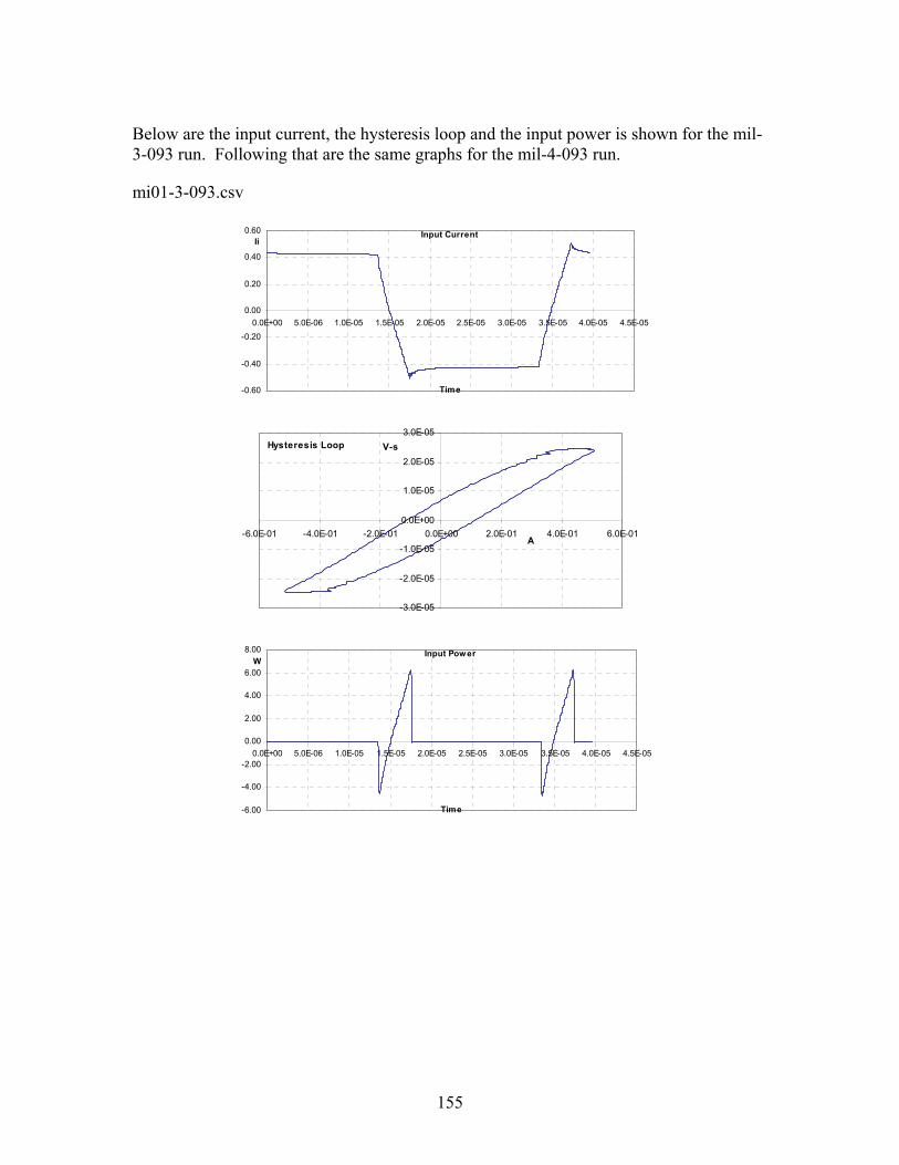
155

Below are the input current, the hysteresis loop and the input power is shown for the mil-3-093 run. Following that are the same graphs for the mil-4-093 run.

mi01-3-093.csv

Input Current

-0.60

-0.40

-0.20

0.00

0.20

0.40

0.60

0.0E+00 5.0E-06 1.0E-05 1.5E-05 2.0E-05 2.5E-05 3.0E-05 3.5E-05 4.0E-05 4.5E-05

Time

Ii

Hysteresis Loop

-3.0E-05

-2.0E-05

-1.0E-05

0.0E+00

1.0E-05

2.0E-05

3.0E-05

-6.0E-01 -4.0E-01 -2.0E-01 0.0E+00 2.0E-01 4.0E-01 6.0E-01A

V-s

Input Power

-6.00

-4.00

-2.00

0.00

2.00

4.00

6.00

8.00

0.0E+00 5.0E-06 1.0E-05 1.5E-05 2.0E-05 2.5E-05 3.0E-05 3.5E-05 4.0E-05 4.5E-05

Time

W

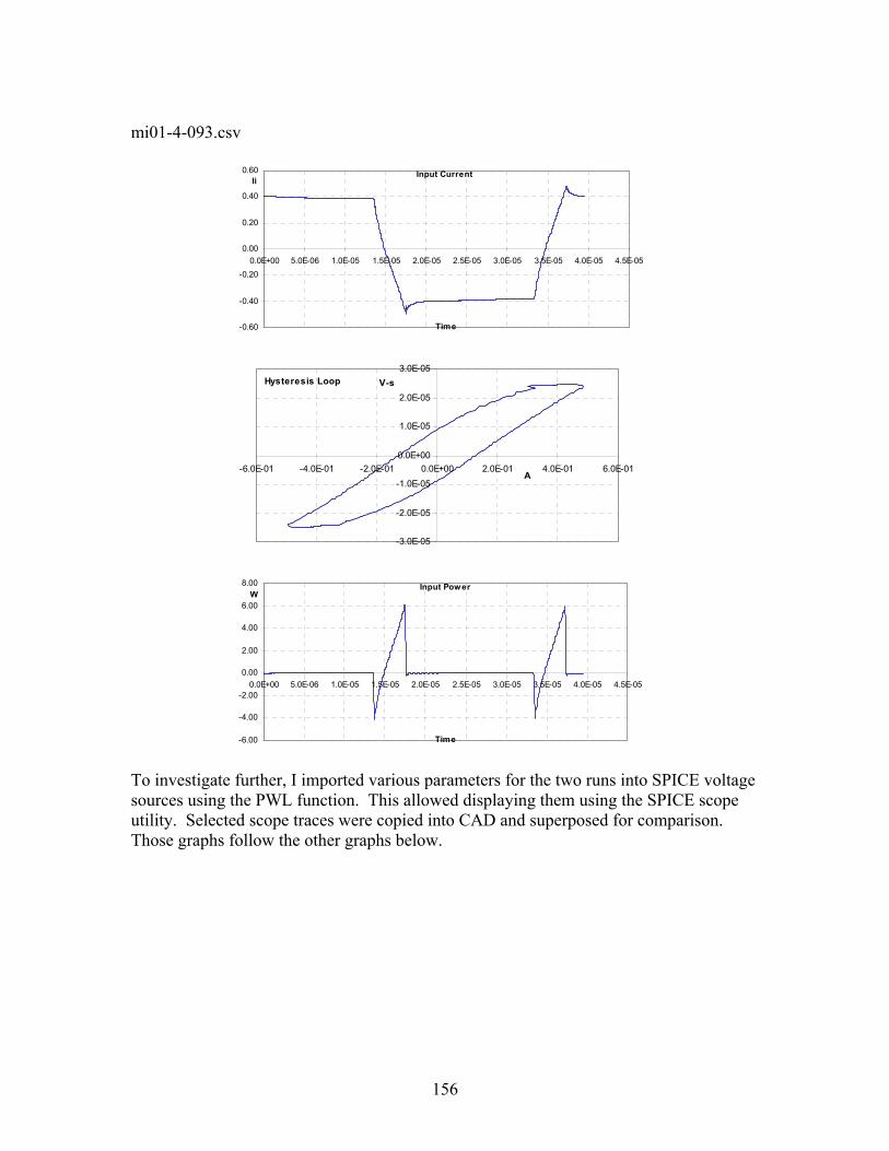
156

mi01-4-093.csv

Input Current

-0.60

-0.40

-0.20

0.00

0.20

0.40

0.60

0.0E+00 5.0E-06 1.0E-05 1.5E-05 2.0E-05 2.5E-05 3.0E-05 3.5E-05 4.0E-05 4.5E-05

Time

Ii

Hysteresis Loop

-3.0E-05

-2.0E-05

-1.0E-05

0.0E+00

1.0E-05

2.0E-05

3.0E-05

-6.0E-01 -4.0E-01 -2.0E-01 0.0E+00 2.0E-01 4.0E-01 6.0E-01A

V-s

Input Power

-6.00

-4.00

-2.00

0.00

2.00

4.00

6.00

8.00

0.0E+00 5.0E-06 1.0E-05 1.5E-05 2.0E-05 2.5E-05 3.0E-05 3.5E-05 4.0E-05 4.5E-05

Time

W

To investigate further, I imported various parameters for the two runs into SPICE voltage sources using the PWL function. This allowed displaying them using the SPICE scope utility. Selected scope traces were copied into CAD and superposed for comparison. Those graphs follow the other graphs below.

157

The graph below shows the sense voltages for the two runs, mi01-3-093 and mil01-4-093, imported into SPICE voltage sources using the PWL function. A possible source of energy difference would be a voltage difference, but they are so close as to be almost indistinguishable. The scope function traces were zoomed to the positive excitation pulse.

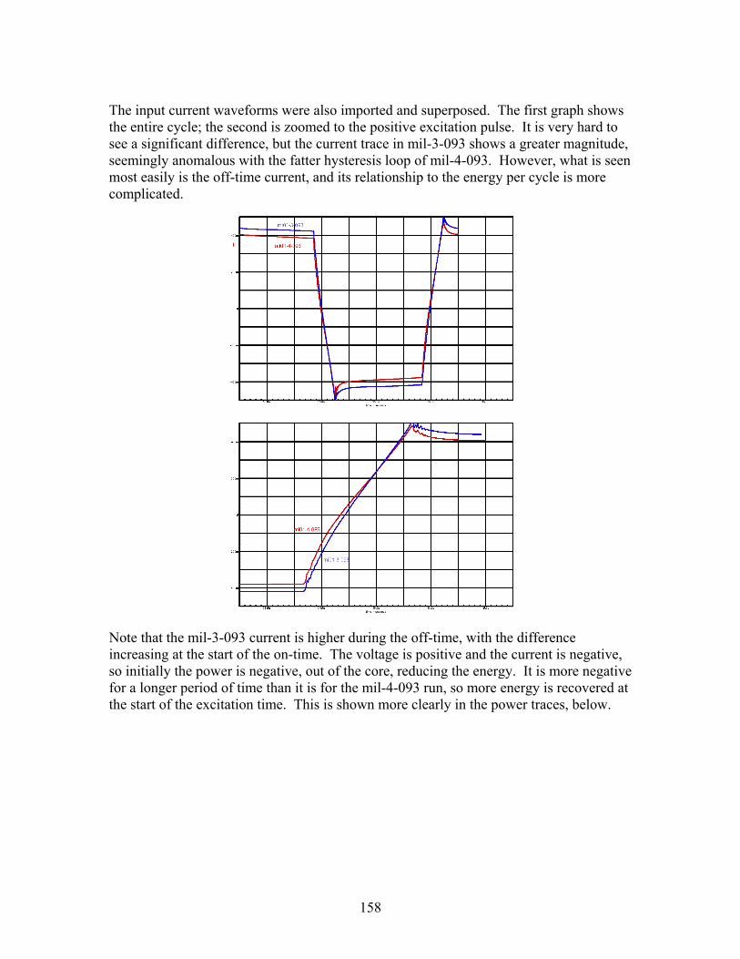
158

The input current waveforms were also imported and superposed. The first graph shows the entire cycle; the second is zoomed to the positive excitation pulse. It is very hard to see a significant difference, but the current trace in mil-3-093 shows a greater magnitude, seemingly anomalous with the fatter hysteresis loop of mil-4-093. However, what is seen most easily is the off-time current, and its relationship to the energy per cycle is more complicated.

Note that the mil-3-093 current is higher during the off-time, with the difference increasing at the start of the on-time. The voltage is positive and the current is negative, so initially the power is negative, out of the core, reducing the energy. It is more negative for a longer period of time than it is for the mil-4-093 run, so more energy is recovered at the start of the excitation time. This is shown more clearly in the power traces, below.

159

The first graph below shows the power into the core for the entire cycle; the second is zoomed to the positive excitation pulse width.

Note that at the beginning of the excitation pulse, the power is negative. It is more negative and it is negative longer for the mi01-3-093 pulse, so much more energy is carried forward. At the trailing edge, where the input energy is positive, the difference is smaller.

The following graph shows the energy into the core for the entire cycle.

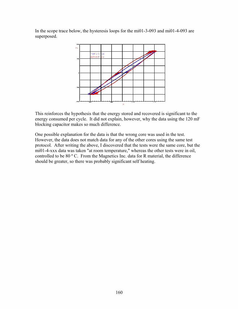
160

In the scope trace below, the hysteresis loops for the mi01-3-093 and mi01-4-093 are superposed.

This reinforces the hypothesis that the energy stored and recovered is significant to the energy consumed per cycle. It did not explain, however, why the data using the 120 mF blocking capacitor makes so much difference.

One possible explanation for the data is that the wrong core was used in the test. However, the data does not match data for any of the other cores using the same test protocol. After writing the above, I discovered that the tests were the same core, but the mi01-4-xxx data was taken "at room temperature," whereas the other tests were in oil, controlled to be 80 º C. From the Magnetics Inc. data for R material, the difference should be greater, so there was probably significant self heating.

161

Another possibility considered was that the much larger blocking capacitor might allow a degree of flux walking, and the hysteresis loops of interest might be a more lossy minor loop. However, a comparison of the mi01-3 and mi01-4 hysteresis loops from the sets images directory shows that both resemble the square wave hysteresis loops, they reasonably well centered, and they approaching but not into saturation. The -039 curves are the reference square waves for the data of interest. The lower voltage loops appear to be fatter as well.

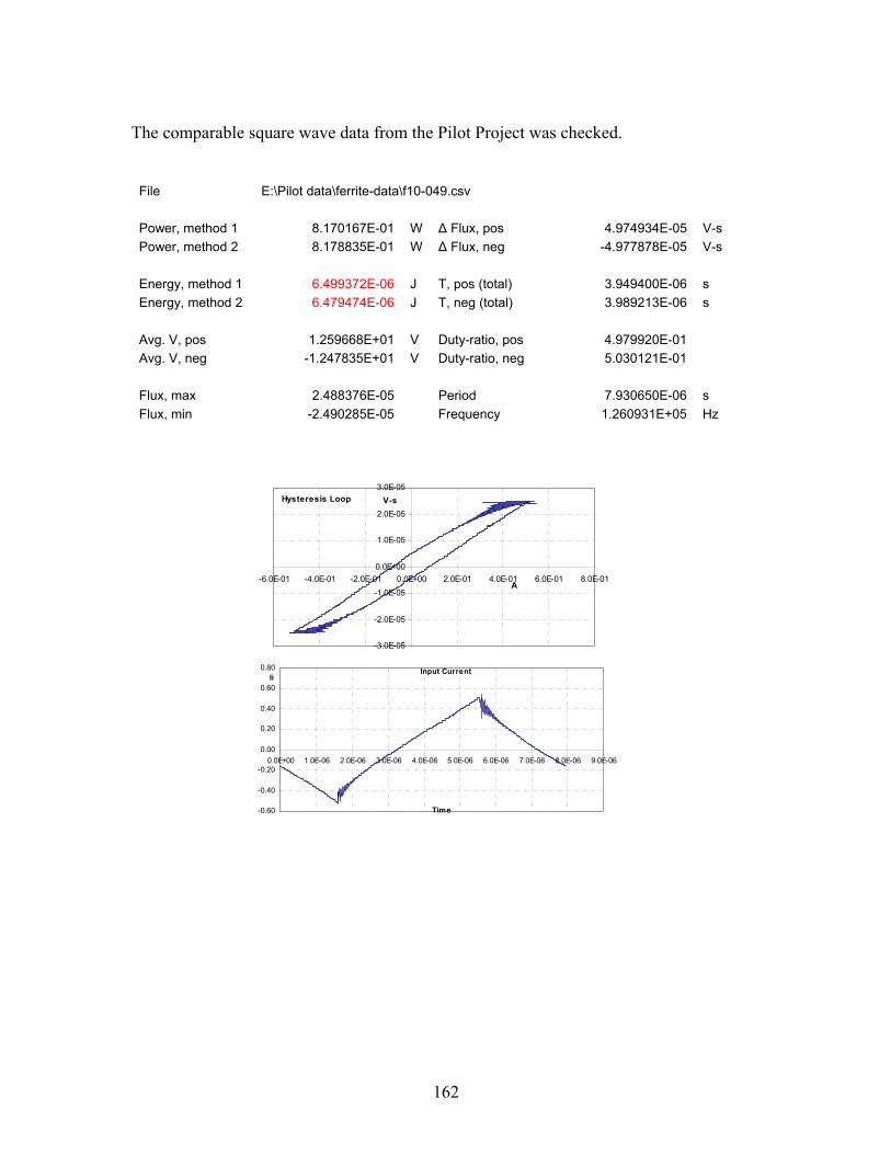
162

The comparable square wave data from the Pilot Project was checked.

File E:\Pilot data\ferrite-data\f10-049.csv Power, method 1 8.170167E-01 W Δ Flux, pos 4.974934E-05 V-s Power, method 2 8.178835E-01 W Δ Flux, neg -4.977878E-05 V-s Energy, method 1 6.499372E-06 J T, pos (total) 3.949400E-06 s Energy, method 2 6.479474E-06 J T, neg (total) 3.989213E-06 s Avg. V, pos 1.259668E+01 V Duty-ratio, pos 4.979920E-01 Avg. V, neg -1.247835E+01 V Duty-ratio, neg 5.030121E-01 Flux, max 2.488376E-05 Period 7.930650E-06 s Flux, min -2.490285E-05 Frequency 1.260931E+05 Hz

Hysteresis Loop

-3.0E-05

-2.0E-05

-1.0E-05

0.0E+00

1.0E-05

2.0E-05

3.0E-05

-6.0E-01 -4.0E-01 -2.0E-01 0.0E+00 2.0E-01 4.0E-01 6.0E-01 8.0E-01A

V-s

Input Current

-0.60

-0.40

-0.20

0.00

0.20

0.40

0.60

0.80

0.0E+00 1.0E-06 2.0E-06 3.0E-06 4.0E-06 5.0E-06 6.0E-06 7.0E-06 8.0E-06 9.0E-06

Time

Ii

163

The square wave Pilot Project data compares closely to the Phase II mi01-3-039 data:

File E:\Phase II Data\sets\mi01-3\scope\mi01-3-039.csv Power, method 1 8.380325E-01 W Δ Flux, pos 4.943937E-05 V-s Power, method 2 8.388997E-01 W Δ Flux, neg -4.939588E-05 V-s Energy, method 1 6.666379E-06 J T, pos (total) 3.989213E-06 s Energy, method 2 6.646142E-06 J T, neg (total) 3.949400E-06 s Avg. V, pos 1.239326E+01 V Duty-ratio, pos 5.030121E-01 Avg. V, neg -1.250719E+01 V Duty-ratio, neg 4.979920E-01 Flux, max 2.472378E-05 Period 7.930650E-06 s Flux, min -2.471559E-05 Frequency 1.260931E+05 Hz

Hysteresis Loop

-3.0E-05

-2.0E-05

-1.0E-05

0.0E+00

1.0E-05

2.0E-05

3.0E-05

-8.0E-01 -6.0E-01 -4.0E-01 -2.0E-01 0.0E+00 2.0E-01 4.0E-01 6.0E-01 8.0E-01A

V-s

Input Current

-0.80

-0.60

-0.40

-0.20

0.00

0.20

0.40

0.60

0.80

0.0E+00 1.0E-06 2.0E-06 3.0E-06 4.0E-06 5.0E-06 6.0E-06 7.0E-06 8.0E-06 9.0E-06

Time

Ii

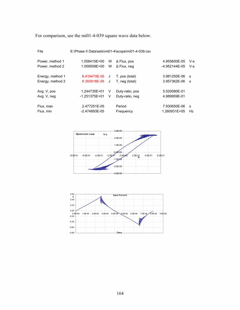
164

For comparison, see the mi01-4-039 square wave data below.

File E:\Phase II Data\sets\mi01-4\scope\mi01-4-039.csv Power, method 1 1.058415E+00 W Δ Flux, pos 4.955600E-05 V-s Power, method 2 1.059509E+00 W Δ Flux, neg -4.952144E-05 V-s Energy, method 1 8.419470E-06 J T, pos (total) 3.981250E-06 s Energy, method 2 8.393918E-06 J T, neg (total) 3.957362E-06 s Avg. V, pos 1.244735E+01 V Duty-ratio, pos 5.020080E-01 Avg. V, neg -1.251375E+01 V Duty-ratio, neg 4.989959E-01 Flux, max 2.477251E-05 Period 7.930650E-06 s Flux, min -2.474893E-05 Frequency 1.260931E+05 Hz

Hysteresis Loop

-3.0E-05

-2.0E-05

-1.0E-05

0.0E+00

1.0E-05

2.0E-05

3.0E-05

-8.0E-01 -6.0E-01 -4.0E-01 -2.0E-01 0.0E+00 2.0E-01 4.0E-01 6.0E-01A

V-s

Input Current

-0.80

-0.60

-0.40

-0.20

0.00

0.20

0.40

0.60

0.0E+00 1.0E-06 2.0E-06 3.0E-06 4.0E-06 5.0E-06 6.0E-06 7.0E-06 8.0E-06 9.0E-06

Time

Ii

165

Comparisons to a SPICE model

I created a SPICE model, below, as explained in Appendix J, Simple SPICE model. I ran the mi01-3-093.csv file in the Excel Tool, which exports the Vi, Ii and Flux data to files accessible by SPICE. These become the PWL function for the three voltage sources with terminals having the same names. When run, the model makes the mi01-3-093 parameters available on the terminals.

I added an inductor L1 and a voltage source Vt set to 0 V. This is the SPICE recommended way to measure current as i(Vt). The inductor and its ammeter are connected to Vi through a terminal, so the model has the same excitation voltage as mi01-3-093.

The purpose of this exercise is to compare the model currents and hysteresis loops to the mi01-3-093 run. To make the difference current easier to see, a behavioral voltage source B1 generates the difference term, v(Ii) –i(Vt). SPICE does not care that I am subtracting a current from a voltage, it just yields the numeric difference.

The first graph below shows the currents Ii and i(Vt) with the difference.

166

The graphs below show the mi01-3-093 current, red, and the model current i(Vt), blue. The green line is the difference. The difference current is green. It is very hard to visualize he the vertical separation of the Ii and i(Vt) lines, so the difference function is important.

The hysteresis loops for Ii vs Flux (red) and i(Vt) vs Flux, blue, are superposed. With only an inductor, the model hysteresis is a straight line.

167

We now add some resistors to the model. The small series resistor R1, 0.12 Ω, models the shallow down-slope seen in the mi01-3-093 current Ii. There is a substantial difference current component seen only during the on-time. This suggests the parallel resistor R1.

The addition of the resistors makes the currents match much more closely. The difference in the sloped portions of the curve is very difficult to see, but is quite evident in the difference current display. Note that the difference currents have about the same time constant when the excitation is applied and when it is removed.

Note that the current step is approximately correct, but the time constant is way off. The error is fairly easy to spot in the relatively flat curve at the off-time. It is about the same when the voltage is applied, but that is very difficult to see without the difference current display.

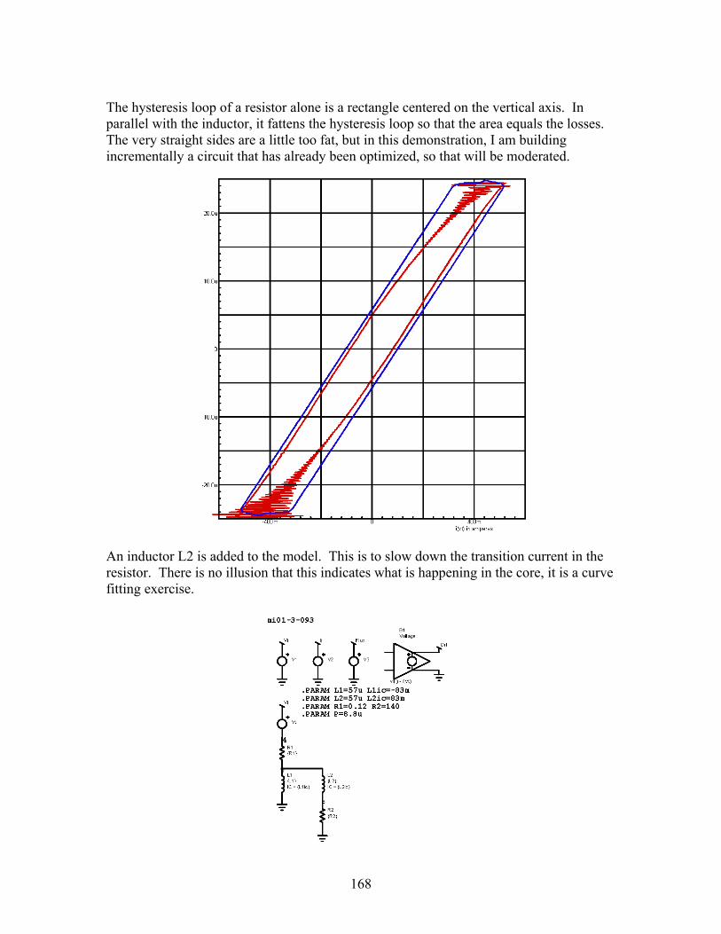
168

The hysteresis loop of a resistor alone is a rectangle centered on the vertical axis. In parallel with the inductor, it fattens the hysteresis loop so that the area equals the losses. The very straight sides are a little too fat, but in this demonstration, I am building incrementally a circuit that has already been optimized, so that will be moderated.

An inductor L2 is added to the model. This is to slow down the transition current in the resistor. There is no illusion that this indicates what is happening in the core, it is a curve fitting exercise.

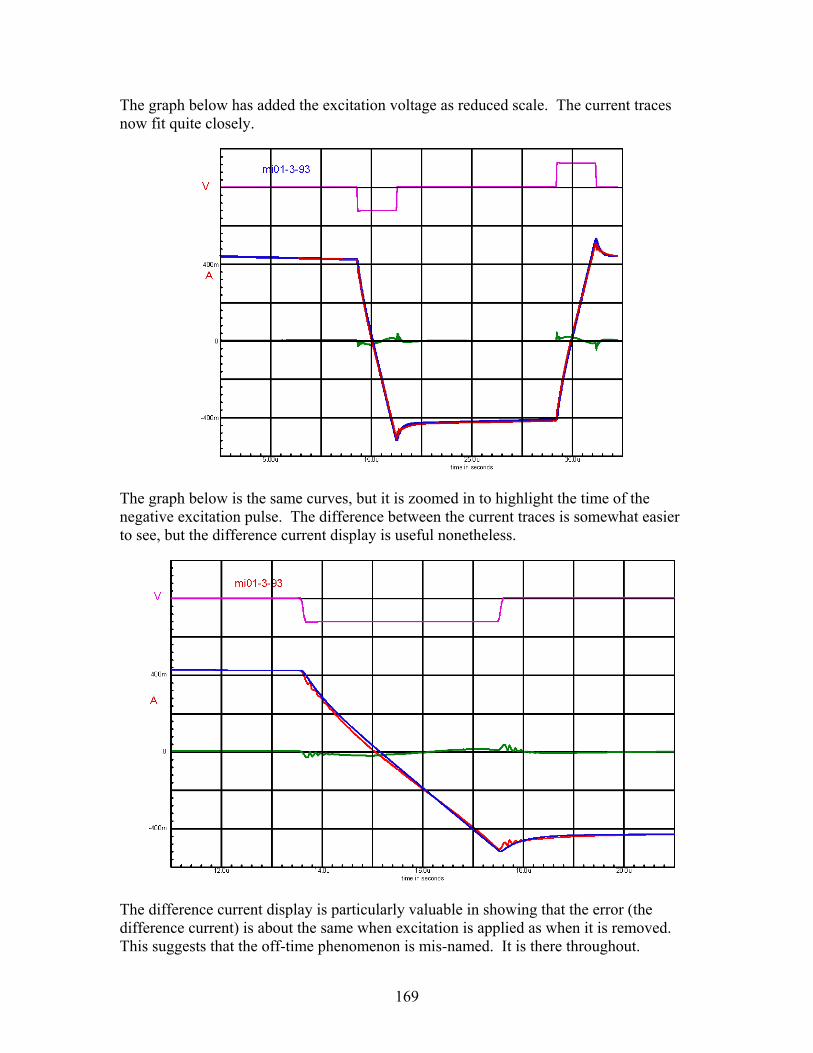
169

The graph below has added the excitation voltage as reduced scale. The current traces now fit quite closely.

The graph below is the same curves, but it is zoomed in to highlight the time of the negative excitation pulse. The difference between the current traces is somewhat easier to see, but the difference current display is useful nonetheless.

The difference current display is particularly valuable in showing that the error (the difference current) is about the same when excitation is applied as when it is removed. This suggests that the off-time phenomenon is mis-named. It is there throughout.

170

The hysteresis loops now are quite close as well. The model has slightly higher current in the corners, and that can be seen in the current traces as well, but it is much more conspicuous in the hysteresis loop. For core loss estimates, the important parameter is the respective areas, and they look to be quite similar.

171

We can now see how the model performs with a different waveform. The file mi01-3-88 is loaded into the Excel Tool and calculated. This exports new data to the PWL files that the SPICE program access when run. Because the period is much shorter, the run time is reset. Also, the initial conditions on the inductors must be reset.

The slight mismatch at in the hysteresis loop of the model (blue) is because one of the initial condition currents is slightly off. That is the starting point of the loop.

172

We now repeat the procedure for the mi01-3-85 run. This one is interesting because the off-time is very short, of the order of the time constant of the current transient. Note that there are two very similar transients, at the start and at the end of the off-time, repeating at the next off-time.

The hysteresis loops match reasonably well, though it is somewhat obscured by the noise in the current waveform.

173

Finally, we use the model with the square-wave, mi01-039. Note that the same transients are present at the transitions, but the magnitude is twice as large. This is reasonable, as the change in voltage going directly from +V to –V is twice what it is goind from +V to 0, then 0 to –V.

The hysteresis loop is still a reasonably good fit.

174

Before becoming too pleased with the model, it is worth stating that it performs less well with the hippo curve. With experience and rigor, I believe that a voltage waveform test protocol can be developed that will reveal the model component parameters in a fairly straightforward manner. Until that expertise is developed, perfecting the model is somewhat like playing "Whac-a-mole."

While not conclusive, this exercise is suggestive that an impedance model can model core losses quite well. The model of this example is quite simple, yet would be useful for hysteretic waveforms of varying off-time.

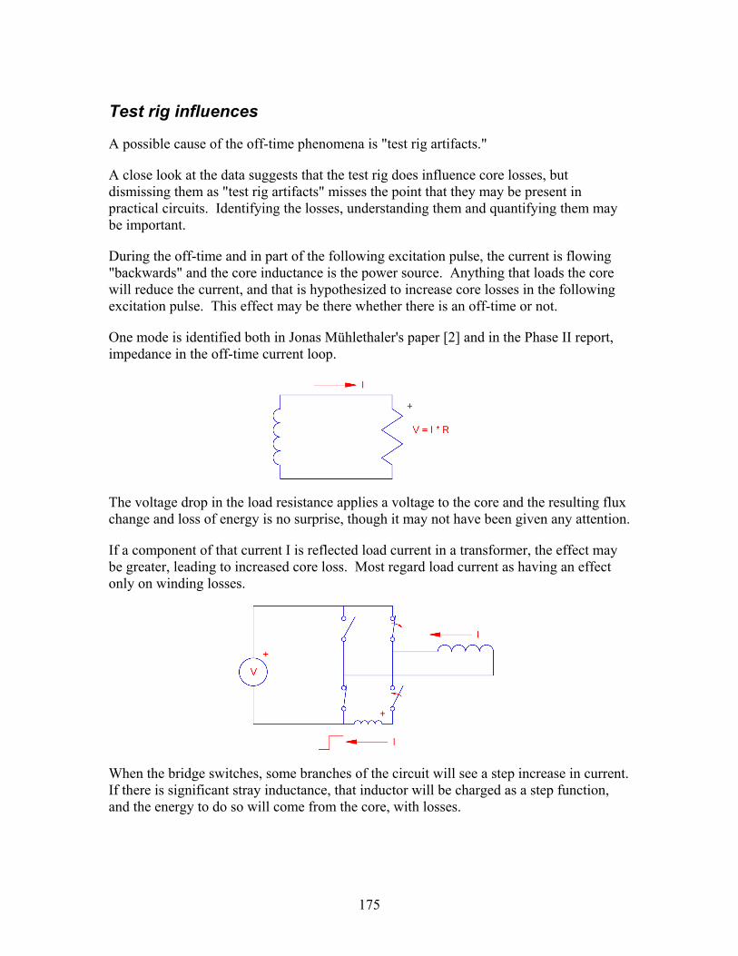
175

Test rig influences

A possible cause of the off-time phenomena is "test rig artifacts."

A close look at the data suggests that the test rig does influence core losses, but dismissing them as "test rig artifacts" misses the point that they may be present in practical circuits. Identifying the losses, understanding them and quantifying them may be important.

During the off-time and in part of the following excitation pulse, the current is flowing "backwards" and the core inductance is the power source. Anything that loads the core will reduce the current, and that is hypothesized to increase core losses in the following excitation pulse. This effect may be there whether there is an off-time or not.

One mode is identified both in Jonas Mühlethaler's paper [2] and in the Phase II report, impedance in the off-time current loop.

The voltage drop in the load resistance applies a voltage to the core and the resulting flux change and loss of energy is no surprise, though it may not have been given any attention.

If a component of that current I is reflected load current in a transformer, the effect may be greater, leading to increased core loss. Most regard load current as having an effect only on winding losses.

When the bridge switches, some branches of the circuit will see a step increase in current. If there is significant stray inductance, that inductor will be charged as a step function, and the energy to do so will come from the core, with losses.

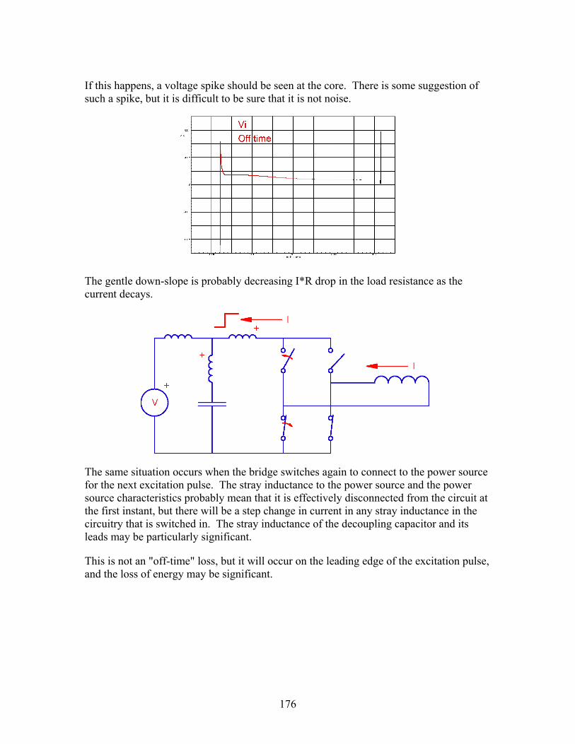
176

If this happens, a voltage spike should be seen at the core. There is some suggestion of such a spike, but it is difficult to be sure that it is not noise.

The gentle down-slope is probably decreasing I*R drop in the load resistance as the current decays.

The same situation occurs when the bridge switches again to connect to the power source for the next excitation pulse. The stray inductance to the power source and the power source characteristics probably mean that it is effectively disconnected from the circuit at the first instant, but there will be a step change in current in any stray inductance in the circuitry that is switched in. The stray inductance of the decoupling capacitor and its leads may be particularly significant.

This is not an "off-time" loss, but it will occur on the leading edge of the excitation pulse, and the loss of energy may be significant.

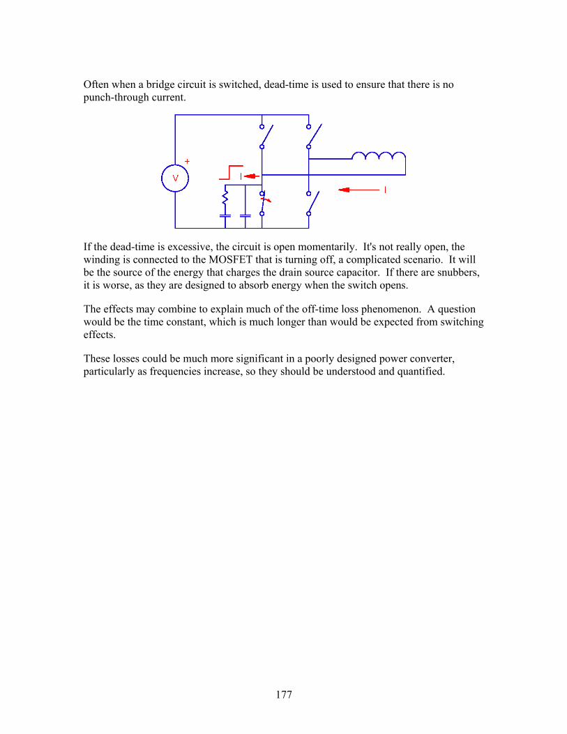
177

Often when a bridge circuit is switched, dead-time is used to ensure that there is no punch-through current.

If the dead-time is excessive, the circuit is open momentarily. It's not really open, the winding is connected to the MOSFET that is turning off, a complicated scenario. It will be the source of the energy that charges the drain source capacitor. If there are snubbers, it is worse, as they are designed to absorb energy when the switch opens.

The effects may combine to explain much of the off-time loss phenomenon. A question would be the time constant, which is much longer than would be expected from switching effects.

These losses could be much more significant in a poorly designed power converter, particularly as frequencies increase, so they should be understood and quantified.

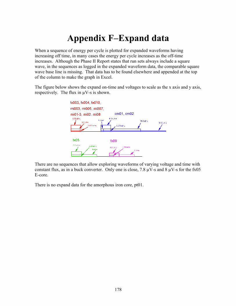
178

Appendix F–Expand data When a sequence of energy per cycle is plotted for expanded waveforms having increasing off time, in many cases the energy per cycle increases as the off-time increases. Although the Phase II Report states that run sets always include a square wave, in the sequences as logged in the expanded waveform data, the comparable square wave base line is missing. That data has to be found elsewhere and appended at the top of the column to make the graph in Excel.

The figure below shows the expand on-time and voltages to scale as the x axis and y axis, respectively. The flux in µV-s is shown.

There are no sequences that allow exploring waveforms of varying voltage and time with constant flux, as in a buck converter. Only one is close, 7.8 µV-s and 8 µV-s for the fx05 E-core.

There is no expand data for the amorphous iron core, pt01.

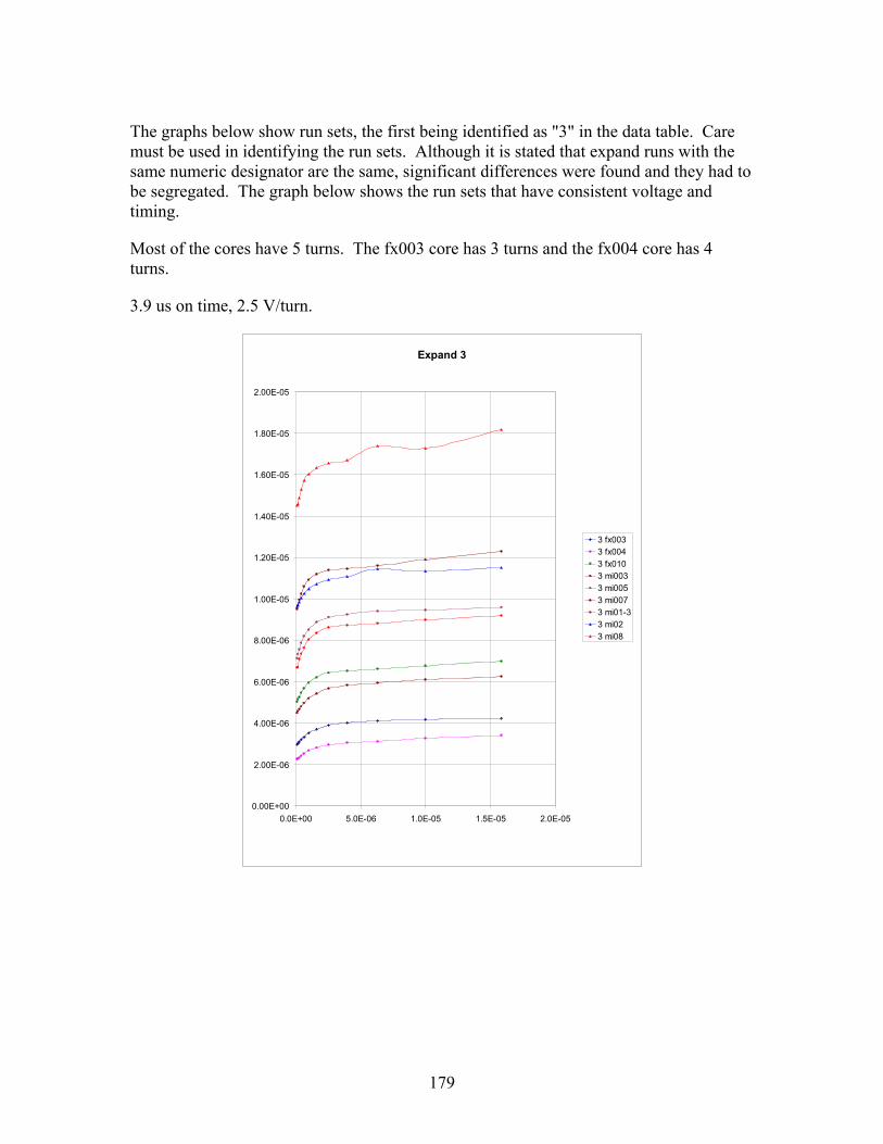
179

The graphs below show run sets, the first being identified as "3" in the data table. Care must be used in identifying the run sets. Although it is stated that expand runs with the same numeric designator are the same, significant differences were found and they had to be segregated. The graph below shows the run sets that have consistent voltage and timing.

Most of the cores have 5 turns. The fx003 core has 3 turns and the fx004 core has 4 turns.

3.9 us on time, 2.5 V/turn.

Expand 3

0.00E+00

2.00E-06

4.00E-06

6.00E-06

8.00E-06

1.00E-05

1.20E-05

1.40E-05

1.60E-05

1.80E-05

2.00E-05

0.0E+00 5.0E-06 1.0E-05 1.5E-05 2.0E-05

3 fx0033 fx0043 fx0103 mi0033 mi0053 mi0073 mi01-33 mi023 mi08

180

3.3 us on time, 1 V/turn

Expand 2

0.00E+00

1.00E-06

2.00E-06

3.00E-06

4.00E-06

5.00E-06

6.00E-06

0.0E+00 5.0E-06 1.0E-05 1.5E-05 2.0E-05

2 fx0032 fx0042 fx0102 mi0032 mi0052 mi0072 mi01-32 mi022 mi08

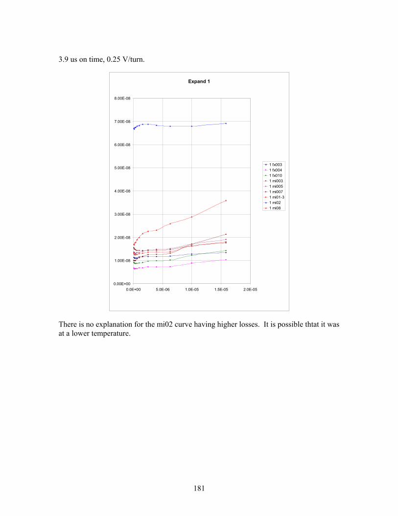
181

3.9 us on time, 0.25 V/turn.

Expand 1

0.00E+00

1.00E-08

2.00E-08

3.00E-08

4.00E-08

5.00E-08

6.00E-08

7.00E-08

8.00E-08

0.0E+00 5.0E-06 1.0E-05 1.5E-05 2.0E-05

1 fx0031 fx0041 fx0101 mi0031 mi0051 mi0071 mi01-31 mi021 mi08

There is no explanation for the mi02 curve having higher losses. It is possible thtat it was at a lower temperature.

182

The data for the Ceramic Magnetics cores Cm01 and Cm02 have different protocols, and were tested with a greater variety of waveforms. The linear plots are shown separately, as an attempt to plot them on one graph had five pairs so much smaller that they hugged the bottom of the graph.

15.8 us on time, 1 V/turn. The cm01 core has 4 turns, the cm02 core has 5 turns.

6 C M OExpand

9.0E-06

1.1E-05

1.3E-05

1.5E-05

1.7E-05

1.9E-05

0.0E+00 2.0E-06 4.0E-06 6.0E-06 8.0E-06 1.0E-05 1.2E-05 1.4E-05 1.6E-05 1.8E-05

6 cm01 6 cm02

3.9 us on time, 2.5 V/turn.

5 C M OExpand

6.0E-076.5E-077.0E-077.5E-078.0E-078.5E-079.0E-079.5E-071.0E-06

0.0E+00 2.0E-06 4.0E-06 6.0E-06 8.0E-06 1.0E-05 1.2E-05 1.4E-05 1.6E-05 1.8E-05

5 cm01 5 cm02

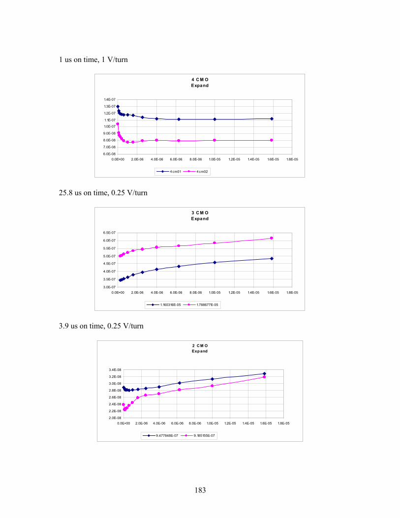
183

1 us on time, 1 V/turn

4 C M OExpand

6.0E-08

7.0E-08

8.0E-08

9.0E-08

1.0E-07

1.1E-07

1.2E-07

1.3E-07

1.4E-07

0.0E+00 2.0E-06 4.0E-06 6.0E-06 8.0E-06 1.0E-05 1.2E-05 1.4E-05 1.6E-05 1.8E-05

4 cm01 4 cm02

25.8 us on time, 0.25 V/turn

3 C M OExpand

3.0E-07

3.5E-07

4.0E-07

4.5E-07

5.0E-07

5.5E-07

6.0E-07

6.5E-07

0.0E+00 2.0E-06 4.0E-06 6.0E-06 8.0E-06 1.0E-05 1.2E-05 1.4E-05 1.6E-05 1.8E-05

1.160316E-05 1.788677E-05

3.9 us on time, 0.25 V/turn

2 C M OExpand

2.0E-08

2.2E-08

2.4E-08

2.6E-08

2.8E-08

3.0E-08

3.2E-08

3.4E-08

0.0E+00 2.0E-06 4.0E-06 6.0E-06 8.0E-06 1.0E-05 1.2E-05 1.4E-05 1.6E-05 1.8E-05

9.477848E-07 9.185155E-07

184

1 us on time, 0.25 V/turn.

1 C M OExpand

3.0E-09

4.0E-09

5.0E-09

6.0E-09

7.0E-09

8.0E-09

9.0E-09

0.0E+00 2.0E-06 4.0E-06 6.0E-06 8.0E-06 1.0E-05 1.2E-05 1.4E-05 1.6E-05 1.8E-05

1.122512E-07 8.035861E-08

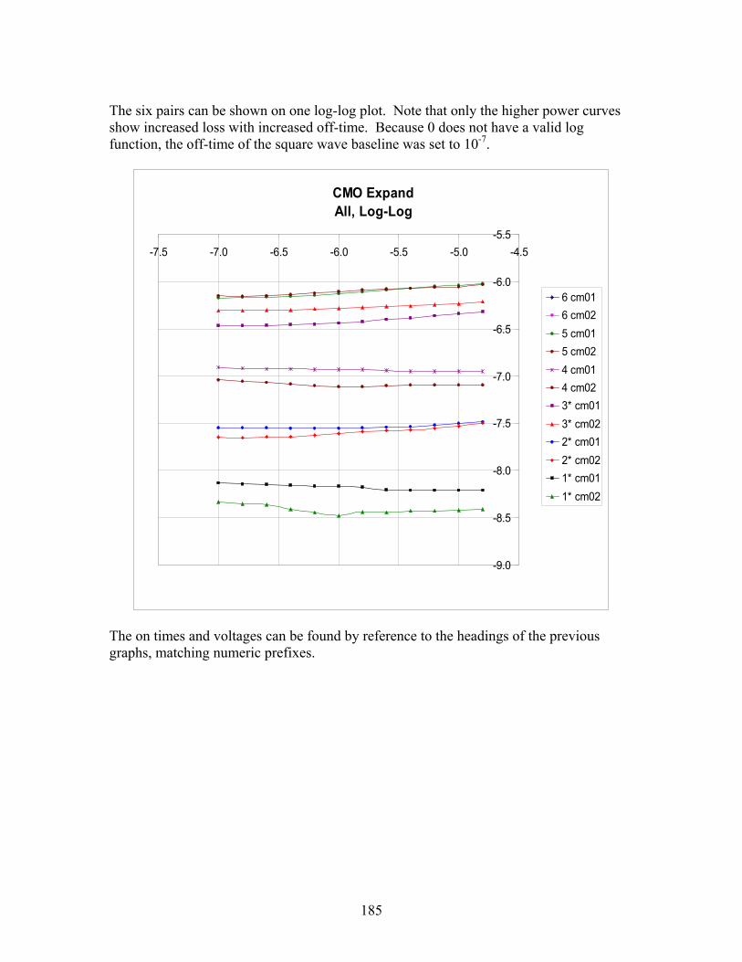
185

The six pairs can be shown on one log-log plot. Note that only the higher power curves show increased loss with increased off-time. Because 0 does not have a valid log function, the off-time of the square wave baseline was set to 10-7.

CMO ExpandAll, Log-Log

-9.0

-8.5

-8.0

-7.5

-7.0

-6.5

-6.0

-5.5-7.5 -7.0 -6.5 -6.0 -5.5 -5.0 -4.5

6 cm016 cm025 cm015 cm024 cm014 cm023* cm013* cm022* cm012* cm021* cm011* cm02

The on times and voltages can be found by reference to the headings of the previous graphs, matching numeric prefixes.

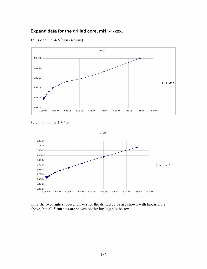
186

Expand data for the drilled core, mi11-1-xxx.

15 us on time, 4 V/turn (4 turns)

5 mi11-1

7.5E-05

8.0E-05

8.5E-05

9.0E-05

9.5E-05

1.0E-04

0.0E+00 2.0E-06 4.0E-06 6.0E-06 8.0E-06 1.0E-05 1.2E-05 1.4E-05 1.6E-05 1.8E-05

5 mi11-1

39.9 us on time, 1 V/turn.

4 mi11-1

2.2E-05

2.3E-05

2.4E-05

2.5E-05

2.6E-05

2.7E-05

2.8E-05

2.9E-05

3.0E-05

3.1E-05

3.2E-05

0.0E+00 2.0E-06 4.0E-06 6.0E-06 8.0E-06 1.0E-05 1.2E-05 1.4E-05 1.6E-05 1.8E-05

4 mi11-1

Only the two highest power curves for the drilled cores are shown with linear plots above, but all 5 run sets are shown on the log-log plot below.

187

Expand Drilled Core-mi11-1Log-Log

-9.5

-8.5

-7.5

-6.5

-5.5

-4.5

-3.5-7.5 -7.0 -6.5 -6.0 -5.5 -5.0 -4.5

1 mi11-12 mi11-13 mi11-14 mi11-15 mi11-1

188

Expand data for the E core, fx05

The data for this E-core is shown separately, as the excitation is different. The fx05 E-core has 6 turns.

The excitations are:

3 fx05, 3.9 us on time, 2 V/turn 2 fx05, 10 us on time, 0.8 V/turn 1 fx05, 3.9 us on time, 0.2 V/turn

3 fx05, 2 fx05-Expand

2.0E-062.2E-062.4E-062.6E-062.8E-063.0E-063.2E-063.4E-063.6E-063.8E-064.0E-06

0.0E+00 5.0E-06 1.0E-05 1.5E-05 2.0E-05

3* fx05 2* fx05

fx05ExpandLog-Log

-8.50

-8.00

-7.50

-7.00

-6.50

-6.00

-5.50

-5.00-8.0 -7.5 -7.0 -6.5 -6.0 -5.5 -5.0 -4.5 -4.0

3* fx05 2* fx05 1* fx05

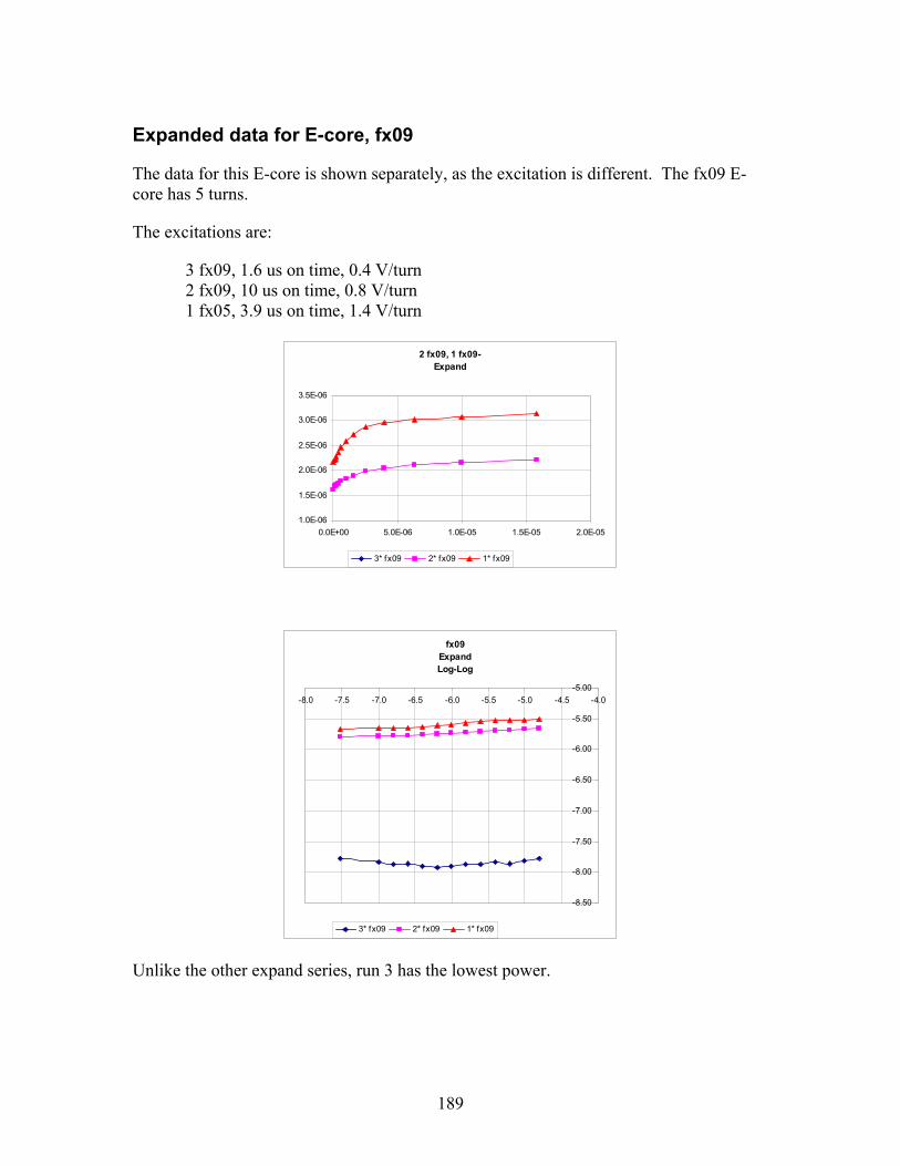
189

Expanded data for E-core, fx09

The data for this E-core is shown separately, as the excitation is different. The fx09 E-core has 5 turns.

The excitations are:

3 fx09, 1.6 us on time, 0.4 V/turn 2 fx09, 10 us on time, 0.8 V/turn 1 fx05, 3.9 us on time, 1.4 V/turn

2 fx09, 1 fx09-Expand

1.0E-06

1.5E-06

2.0E-06

2.5E-06

3.0E-06

3.5E-06

0.0E+00 5.0E-06 1.0E-05 1.5E-05 2.0E-05

3* fx09 2* fx09 1* fx09

fx09ExpandLog-Log

-8.50

-8.00

-7.50

-7.00

-6.50

-6.00

-5.50

-5.00-8.0 -7.5 -7.0 -6.5 -6.0 -5.5 -5.0 -4.5 -4.0

3* fx09 2* fx09 1* fx09

Unlike the other expand series, run 3 has the lowest power.

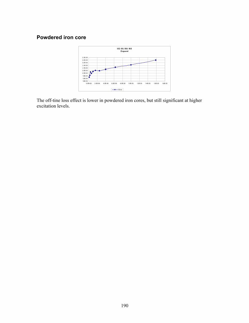
190

Powdered iron core

i02-60,156-165Expand

1.8E-03

1.9E-03

1.9E-03

2.0E-03

2.0E-03

2.1E-03

2.1E-03

2.2E-03

2.2E-03

2.3E-03

0.0E+00 2.0E-06 4.0E-06 6.0E-06 8.0E-06 1.0E-05 1.2E-05 1.4E-05 1.6E-05 1.8E-05

i02 ex

The off-tine loss effect is lower in powdered iron cores, but still significant at higher excitation levels.

191

Appendix G–Hippo data The Hippo waveform is characterized by a pulse of one polarity immediately followed by an equal pulse of the opposite polarity.

mi01-3-110

Input Voltagei

-2.00

-1.50

-1.00

-0.50

0.00

0.50

1.00

1.50

2.00

0.0E+00 2.0E-06 4.0E-06 6.0E-06 8.0E-06 1.0E-05 1.2E-05 1.4E-05

Time

Vi

Flux

-3.0E-06

-2.0E-06

-1.0E-06

0.0E+00

1.0E-06

2.0E-06

3.0E-06

0.0E+00 2.0E-06 4.0E-06 6.0E-06 8.0E-06 1.0E-05 1.2E-05 1.4E-05

Time

V-s

The concept is to reduce the input current to 0, so that there is no energy carried forward as E = ½ I2 L.

Input Current

-0.08

-0.06

-0.04

-0.02

0.00

0.02

0.04

0.06

0.08

0.0E+00 2.0E-06 4.0E-06 6.0E-06 8.0E-06 1.0E-05 1.2E-05 1.4E-05

Time

Ii

Input Power

-0.10

-0.08

-0.06-0.04

-0.02

0.00

0.02

0.04

0.060.08

0.10

0.12

0.0E+00 2.0E-06 4.0E-06 6.0E-06 8.0E-06 1.0E-05 1.2E-05 1.4E-05

Time

W

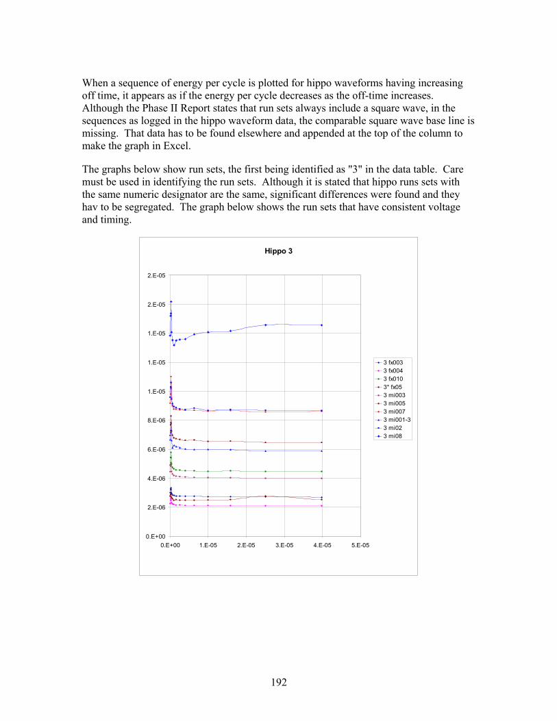
192

When a sequence of energy per cycle is plotted for hippo waveforms having increasing off time, it appears as if the energy per cycle decreases as the off-time increases. Although the Phase II Report states that run sets always include a square wave, in the sequences as logged in the hippo waveform data, the comparable square wave base line is missing. That data has to be found elsewhere and appended at the top of the column to make the graph in Excel.

The graphs below show run sets, the first being identified as "3" in the data table. Care must be used in identifying the run sets. Although it is stated that hippo runs sets with the same numeric designator are the same, significant differences were found and they hav to be segregated. The graph below shows the run sets that have consistent voltage and timing.

Hippo 3

0.E+00

2.E-06

4.E-06

6.E-06

8.E-06

1.E-05

1.E-05

1.E-05

2.E-05

2.E-05

0.E+00 1.E-05 2.E-05 3.E-05 4.E-05 5.E-05

3 fx0033 fx0043 fx0103* fx053 mi0033 mi0053 mi0073 mi001-33 mi023 mi08

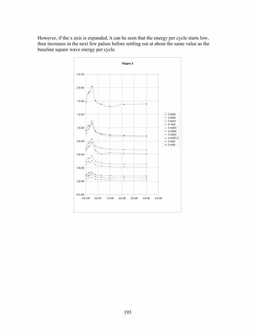
193

However, if the x axis is expanded, it can be seen that the energy per cycle starts low, then increases in the next few pulses before settling out at about the same value as the baseline square wave energy per cycle.

Hippo 3

0.E+00

2.E-06

4.E-06

6.E-06

8.E-06

1.E-05

1.E-05

1.E-05

2.E-05

2.E-05

0.E+00 5.E-07 1.E-06 2.E-06 2.E-06 3.E-06 3.E-06

3 fx0033 fx0043 fx0103* fx053 mi0033 mi0053 mi0073 mi001-33 mi023 mi08

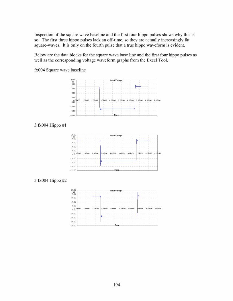
194

Inspection of the square wave baseline and the first four hippo pulses shows why this is so. The first three hippo pulses lack an off-time, so they are actually increasingly fat square-waves. It is only on the fourth pulse that a true hippo waveform is evident.

Below are the data blocks for the square wave base line and the first four hippo pulses as well as the corresponding voltage waveform graphs from the Excel Tool.

fx004 Square wave baseline

Input Voltagei

-20.00

-15.00

-10.00

-5.00

0.00

5.00

10.00

15.00

20.00

0.0E+00 1.0E-06 2.0E-06 3.0E-06 4.0E-06 5.0E-06 6.0E-06 7.0E-06 8.0E-06 9.0E-06

Time

Vi

3 fx004 Hippo #1

Input Voltagei

-25.00

-20.00

-15.00

-10.00

-5.00

0.00

5.00

10.00

15.00

20.00

0.0E+00 1.0E-06 2.0E-06 3.0E-06 4.0E-06 5.0E-06 6.0E-06 7.0E-06 8.0E-06 9.0E-06

Time

Vi

3 fx004 Hippo #2

Input Voltagei

-25.00

-20.00

-15.00

-10.00

-5.00

0.00

5.00

10.00

15.00

20.00

0.0E+00 1.0E-06 2.0E-06 3.0E-06 4.0E-06 5.0E-06 6.0E-06 7.0E-06 8.0E-06 9.0E-06

Time

Vi

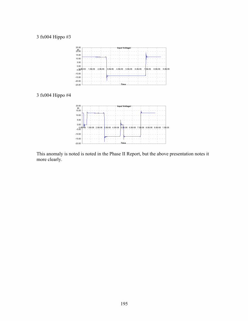
195

3 fx004 Hippo #3

Input Voltagei

-25.00

-20.00

-15.00

-10.00

-5.00

0.00

5.00

10.00

15.00

20.00

25.00

0.0E+00 1.0E-06 2.0E-06 3.0E-06 4.0E-06 5.0E-06 6.0E-06 7.0E-06 8.0E-06 9.0E-06

Time

Vi

3 fx004 Hippo #4

Input Voltagei

-20.00

-15.00

-10.00

-5.00

0.00

5.00

10.00

15.00

20.00

0.0E+00 1.0E-06 2.0E-06 3.0E-06 4.0E-06 5.0E-06 6.0E-06 7.0E-06 8.0E-06 9.0E-06 1.0E-05

Time

Vi

This anomaly is noted is noted in the Phase II Report, but the above presentation notes it more clearly.

196

In the hippo sequences that follow, the first three pulses of the hippo sequence are deleted. The first pulse is the square wave baseline.

If there is any energy reduction, it is slight and inconsistent. The conclusion is that for the hippo waveforms, the length of the off time does not affect the core loss per cycle, as expected.

Hippo 3D

0.E+00

2.E-06

4.E-06

6.E-06

8.E-06

1.E-05

1.E-05

1.E-05

2.E-05

0.0E+00 5.0E-07 1.0E-06 1.5E-06 2.0E-06 2.5E-06 3.0E-06

3 fx0033 fx0043 fx0103* fx053 mi0033 mi0053 mi0073 mi001-33 mi023 mi08

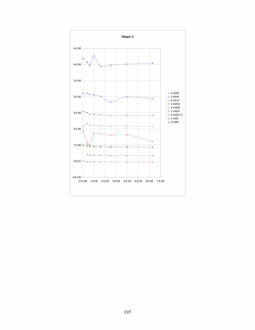
197

Hippo 2

0.E+00

5.E-07

1.E-06

2.E-06

2.E-06

3.E-06

3.E-06

4.E-06

4.E-06

0.E+00 1.E-06 2.E-06 3.E-06 4.E-06 5.E-06 6.E-06 7.E-06

2 fx0033 fx0042 fx0102 mi0032 mi0052 mi0072 mi001-32 mi022 mi08

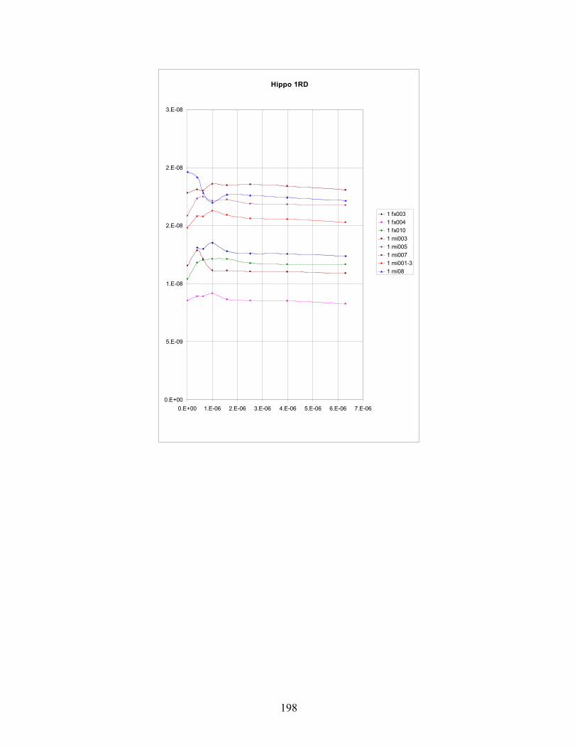
198

Hippo 1RD

0.E+00

5.E-09

1.E-08

2.E-08

2.E-08

3.E-08

0.E+00 1.E-06 2.E-06 3.E-06 4.E-06 5.E-06 6.E-06 7.E-06

1 fx0031 fx0041 fx0101 mi0031 mi0051 mi0071 mi001-31 mi08

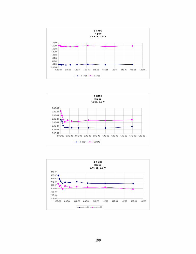
199

6 C M OH ippo

7.89 us, 3 .9 V

9.0E-06

1.0E-05

1.1E-05

1.2E-05

1.3E-05

1.4E-05

1.5E-05

1.6E-05

1.7E-05

0.0E+00 2.0E-06 4.0E-06 6.0E-06 8.0E-06 1.0E-05 1.2E-05 1.4E-05 1.6E-05 1.8E-05

6 cm01 6 cm02

5 C M OH ippo

1.9us, 3 .9 V

6.0E-07

6.2E-07

6.4E-07

6.6E-07

6.8E-07

7.0E-07

7.2E-07

7.4E-07

0.0E+00 2.0E-06 4.0E-06 6.0E-06 8.0E-06 1.0E-05 1.2E-05 1.4E-05 1.6E-05 1.8E-05

5 cm01 5 cm02

4 C M OH ippo

0.46 us, 3 .9 V

6.0E-08

7.0E-08

8.0E-08

9.0E-08

1.0E-07

1.1E-07

1.2E-07

1.3E-07

1.4E-07

0.0E+00 2.0E-06 4.0E-06 6.0E-06 8.0E-06 1.0E-05 1.2E-05 1.4E-05 1.6E-05 1.8E-05

4 cm01 4 cm02

200

3 C M OH ippo

7.9 us, 1 V

3.0E-07

3.5E-07

4.0E-07

4.5E-07

5.0E-07

5.5E-07

0.0E+00 2.0E-06 4.0E-06 6.0E-06 8.0E-06 1.0E-05 1.2E-05

2 C M OHippo

1.9 us, 1 V

2.0E-08

2.2E-08

2.4E-08

2.6E-08

2.8E-08

3.0E-08

3.2E-08

0.0E+00 2.0E-06 4.0E-06 6.0E-06 8.0E-06 1.0E-05 1.2E-05

1 C M OH ippo

0.55 us, 1 V

3.0E-09

4.0E-09

5.0E-09

6.0E-09

7.0E-09

8.0E-09

9.0E-09

0.0E+00 2.0E-06 4.0E-06 6.0E-06 8.0E-06 1.0E-05 1.2E-05

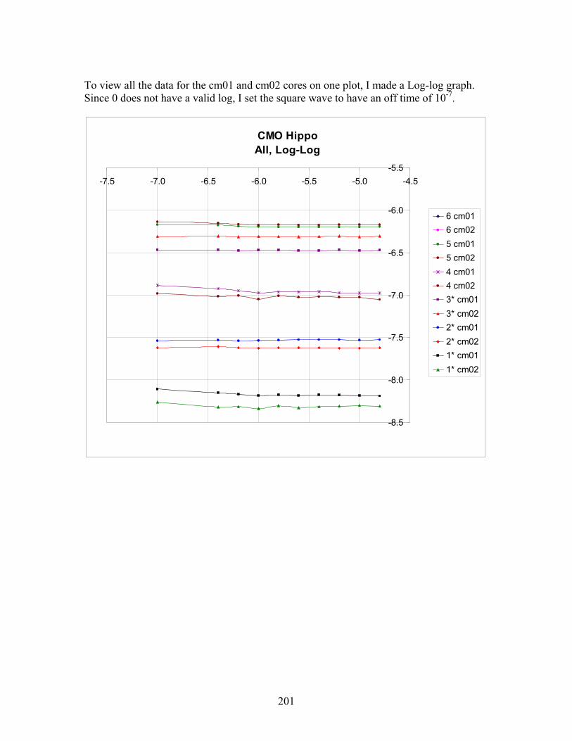
201

To view all the data for the cm01 and cm02 cores on one plot, I made a Log-log graph. Since 0 does not have a valid log, I set the square wave to have an off time of 10-7.

CMO HippoAll, Log-Log

-8.5

-8.0

-7.5

-7.0

-6.5

-6.0

-5.5-7.5 -7.0 -6.5 -6.0 -5.5 -5.0 -4.5

6 cm016 cm025 cm015 cm024 cm014 cm023* cm013* cm022* cm012* cm021* cm011* cm02

202

Appendix H Drilled core data One hypothesis for the off time loss was that the flux in the core might change state after the excitation is removed. With approximately zero nominal volts, the total flux would not be expected to change significantly, but the flux could migrate within the core from one region to another. The drilled core experiments showed that this hypothesis is not substantiated.

To test this hypothesis, a core was drilled through so that test windings could be inserted. Originally, it was planned to drill four holes from each direction (side to side and outside to inside).

A scheme was developed to allow intersecting wires to make an internal connection. If implemented, flux change (voltage) of any of 25 cross-sectional areas could be isolated.

Two more diagonal holes were planned from the outside, meeting within the core, to see if there was a helical component to the flux.

A vendor had promised to supply the drilled core for test, but was unable to perform, so John Harris had to make arrangements himself. Drilling proved to be much more difficult that thought, so the compromise was to drill two holes from each direction and not to drill the diagonal holes.

Time and budget constraints also prevented taking data with intersecting wires.

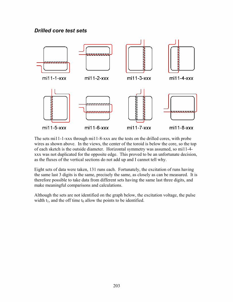
203

Drilled core test sets

The sets mi11-1-xxx through mi11-8-xxx are the tests on the drilled cores, with probe wires as shown above. In the views, the center of the toroid is below the core, so the top of each sketch is the outside diameter. Horizontal symmetry was assumed, so mi11-4-xxx was not duplicated for the opposite edge. This proved to be an unfortunate decision, as the fluxes of the vertical sections do not add up and I cannot tell why.

Eight sets of data were taken, 131 runs each. Fortunately, the excitation of runs having the same last 3 digits is the same, precisely the same, as closely as can be measured. It is therefore possible to take data from different sets having the same last three digits, and make meaningful comparisons and calculations.

Although the sets are not identified on the graph below, the excitation voltage, the pulse width t1, and the off time t0 allow the points to be identified.

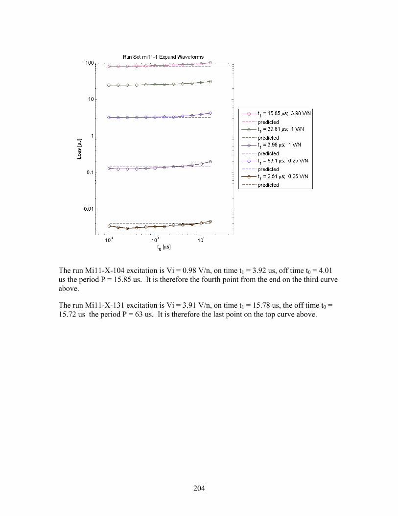
204

The run Mi11-X-104 excitation is Vi = 0.98 V/n, on time t1 = 3.92 us, off time t0 = 4.01 us the period P = 15.85 us. It is therefore the fourth point from the end on the third curve above.

The run Mi11-X-131 excitation is Vi = 3.91 V/n, on time t1 = 15.78 us, the off time t0 = 15.72 us the period P = 63 us. It is therefore the last point on the top curve above.

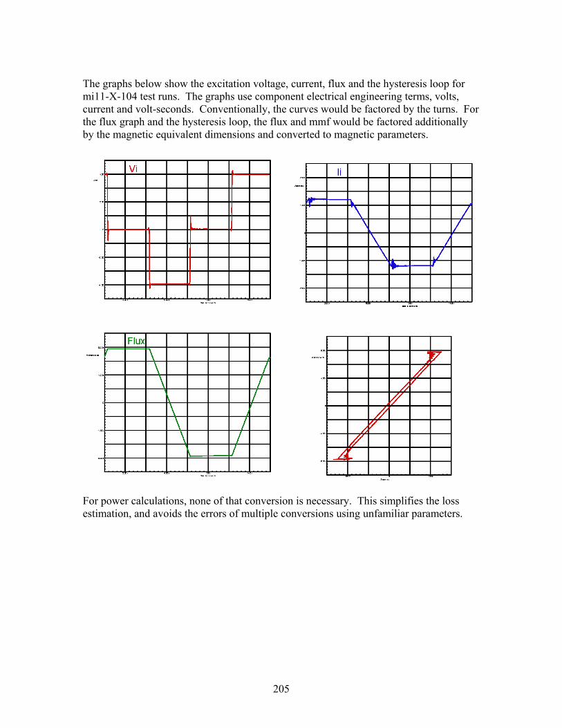
205

The graphs below show the excitation voltage, current, flux and the hysteresis loop for mi11-X-104 test runs. The graphs use component electrical engineering terms, volts, current and volt-seconds. Conventionally, the curves would be factored by the turns. For the flux graph and the hysteresis loop, the flux and mmf would be factored additionally by the magnetic equivalent dimensions and converted to magnetic parameters.

For power calculations, none of that conversion is necessary. This simplifies the loss estimation, and avoids the errors of multiple conversions using unfamiliar parameters.

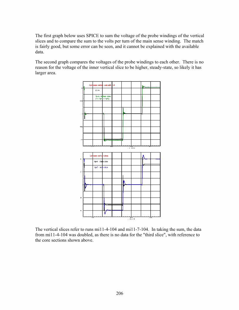
206

The first graph below uses SPICE to sum the voltage of the probe windings of the vertical slices and to compare the sum to the volts per turn of the main sense winding. The match is fairly good, but some error can be seen, and it cannot be explained with the available data.

The second graph compares the voltages of the probe windings to each other. There is no reason for the voltage of the inner vertical slice to be higher, steady-state, so likely it has larger area.

The vertical slices refer to runs mi11-4-104 and mi11-7-104. In taking the sum, the data from mi11-4-104 was doubled, as there is no data for the "third slice", with reference to the core sections shown above.

207

The first graph below uses SPICE to sum the voltages of the probe windings of the horizontal slices and to compare the sum to the volts per turn of the main sense winding. The match is so good that the curves are indistinguishable.

The second graph compares the voltages of the probe windings. It is not expected that the probe voltage of the central probe would be somewhat grater than the probe voltage of the inner winding, steady-state, so likely it has larger area.

The horizontal slices refer to runs mi11-1-104, mi11-6-104 and mi11-2-104.

208

The graphs below show the excitation voltage, current, flux and the hysteresis loop for mi11-X-131 test runs. The graphs use component electrical engineering terms, volts, current and volt-seconds.

209

The current and voltage during the off time are shown below with expanded scale. As can be seen in the graphs on the previous page, the current ramp is quite small and the voltage is very low. The small voltage is positive and the current is negative, so that is power out of the core, but the amount of power is too small to account for the off time loss phenomena.

Two loss components are visible. A short exponential reduction in current is followed by a long linear ramp. The latter is probably the very small IR drop of the circuit resistance and the circulating current. The initial exponential current drop probably accounts for most of the lost energy as a reduction of ½ I2L. The red reference lines were added in CAD.

The flux changes revealed by the embedded windings do not appear to be a significant factor in explaining the off time loss phenomena. They are small, and the timing is not consistent.

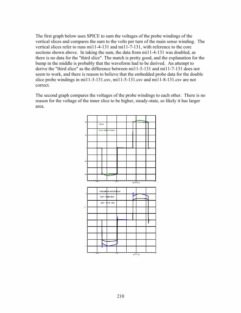
210

The first graph below uses SPICE to sum the voltages of the probe windings of the vertical slices and compares the sum to the volts per turn of the main sense winding. The vertical slices refer to runs mi11-4-131 and mi11-7-131, with reference to the core sections shown above. In taking the sum, the data from mi11-4-131 was doubled, as there is no data for the "third slice". The match is pretty good, and the explanation for the bump in the middle is probably that the waveform had to be derived. An attempt to derive the "third slice" as the difference between mi11-5-131 and mi11-7-131 does not seem to work, and there is reason to believe that the embedded probe data for the double slice probe windings in mi11-3-131.csv, mi11-5-131.csv and mi11-8-131.csv are not correct.

The second graph compares the voltages of the probe windings to each other. There is no reason for the voltage of the inner slice to be higher, steady-state, so likely it has larger area.

211

The first graph below uses SPICE to sum the voltages of the probe windings of the horizontal slices and compares it to the sum to the volts per turn of the main sense winding. The match is so good that the curves are indistinguishable.

The second graph compares the voltages of the probe windings to each other. From the mi11-X-104 data above, it is likely that the central slice has larger area, but its bump up in voltage while the voltage of outer slice goes down is unexpected. Note that the flux goes through zero half way through the pulse. The respective voltages are differences in dφ/dt, so it is apparent that the flux distribution is different at low flux.

The horizontal slices refer to runs mi11-1-131, mi11-6-131 and mi11-2-131.

212

The graphs below show the probe winding voltages during the off time, the first graph showing the vertical slices and the second graph showing the horizontal slices.

The voltages are extremely small and the timing is inconsistent with their being a significant factor in the explanation of the off time losses.

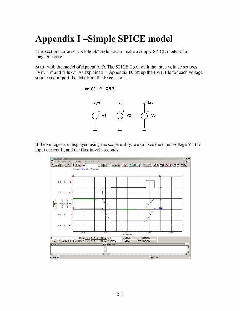
213

Appendix I –Simple SPICE model This section narrates "cook book" style how to make a simple SPICE model of a magnetic core.

Start- with the model of Appendix D, The SPICE Tool, with the three voltage sources "Vi", "Ii" and "Flux." As explained in Appendix D, set up the PWL file for each voltage source and import the data from the Excel Tool.

If the voltages are displayed using the scope utility, we can see the input voltage Vi, the input current Ii, and the flux in volt-seconds:

214

To begin building the SPICE model, add an inductor, and connect it to Vi using a terminal.

Note that I set the value of the inductor L1 to L1, and created a .PARAM statement to set its value. This is unimportant, just my preference. The value of L1 was set by trial and error.

Run the SPICE model, and display the currents Ii and i(L1)

Note the current offset. The exact value can be read from the cursor at the bottom of the screen. This must be added as an "initial condition" for the inductor L1.

215

I added as a .PARAM L1ic = 438.1 m. I also added a .PARAM P=39.5u. P is the period, and can be used to set the run time in the Simulation Setup.

Now the currents look like this:

Next, I added another voltage source set at 0 V and named it "Vt," to measure current, a SPICE recommended procedure. I also added a behavioral voltage source with a ground and a terminal "Dif". The formula for the behavioral voltage source is v(Ii) – i(Vt). SPICE does not care that I am subtracting a current from a voltage; it just uses the values of each. This allows me to see how good the model is as I add components.

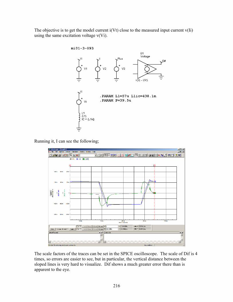
216

The objective is to get the model current i(Vt) close to the measured input current v(Ii) using the same excitation voltage v(Vi).

Running it, I can see the following;

The scale factors of the traces can be set in the SPICE oscilloscope. The scale of Dif is 4 times, so errors are easier to see, but in particular, the vertical distance between the sloped lines is very hard to visualize. Dif shows a much greater error there than is apparent to the eye.

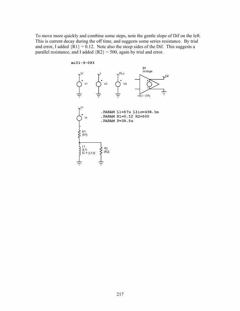
217

To move more quickly and combine some steps, note the gentle slope of Dif on the left. This is current decay during the off time, and suggests some series resistance. By trial and error, I added R1 = 0.12. Note also the steep sides of the Dif. This suggests a parallel resistance, and I added R2 = 500, again by trial and error.

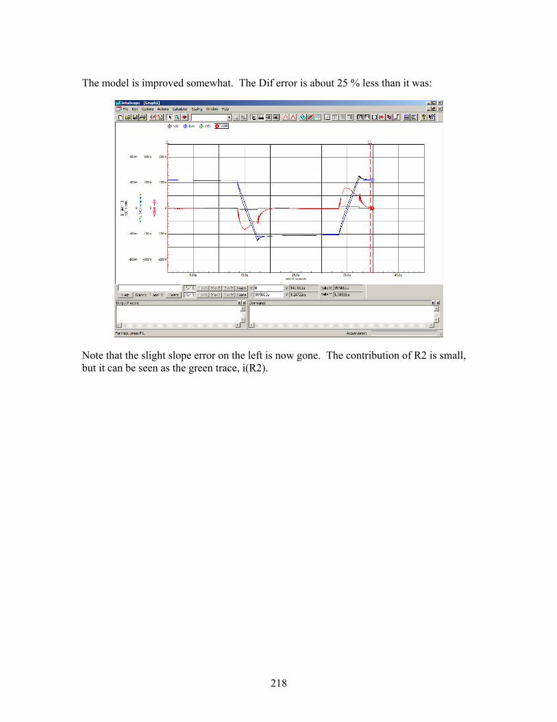
218

The model is improved somewhat. The Dif error is about 25 % less than it was:

Note that the slight slope error on the left is now gone. The contribution of R2 is small, but it can be seen as the green trace, i(R2).

219

There is an exponential current increase as the excitation voltage is applied, and an exponential current decrease after the voltage is removed. This can be seen in the v(Ii) trace, but much more clearly in the Dif trace. A series R-L circuit is added, R3 = 180 and L2 = 80u.

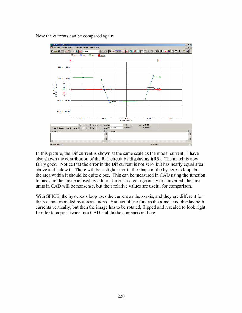
220

Now the currents can be compared again:

In this picture, the Dif current is shown at the same scale as the model current. I have also shown the contribution of the R-L circuit by displaying i(R3). The match is now fairly good. Notice that the error in the Dif current is not zero, but has nearly equal area above and below 0. There will be a slight error in the shape of the hysteresis loop, but the area within it should be quite close. This can be measured in CAD using the function to measure the area enclosed by a line. Unless scaled rigorously or converted, the area units in CAD will be nonsense, but their relative values are useful for comparison.

With SPICE, the hysteresis loop uses the current as the x-axis, and they are different for the real and modeled hysteresis loops. You could use flux as the x-axis and display both currents vertically, but then the image has to be rotated, flipped and rescaled to look right. I prefer to copy it twice into CAD and do the comparison there.

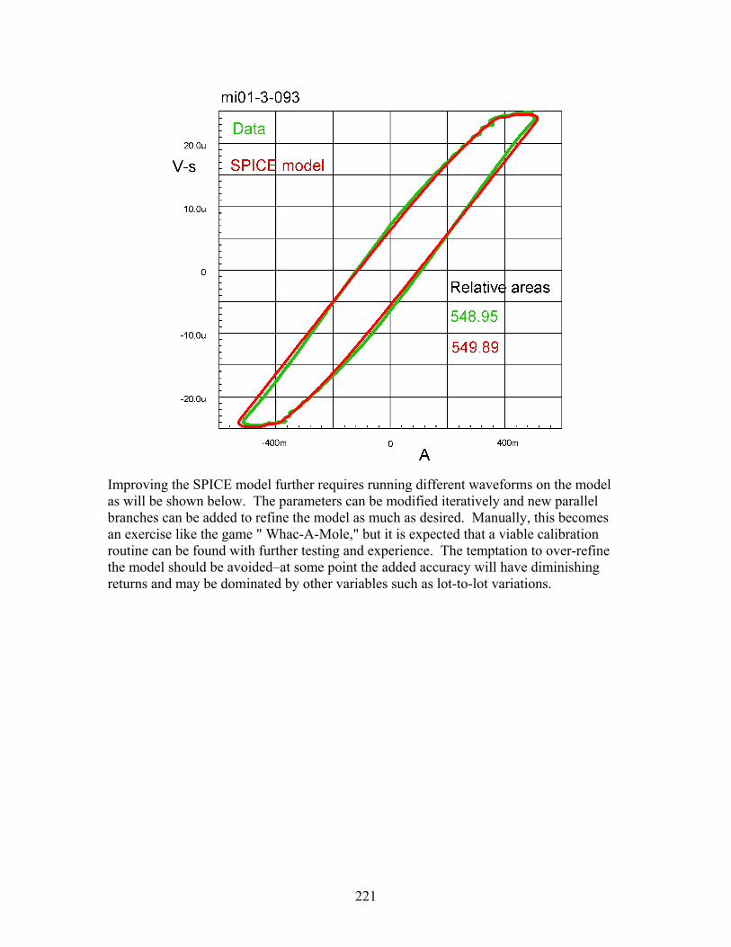
221

Improving the SPICE model further requires running different waveforms on the model as will be shown below. The parameters can be modified iteratively and new parallel branches can be added to refine the model as much as desired. Manually, this becomes an exercise like the game " Whac-A-Mole," but it is expected that a viable calibration routine can be found with further testing and experience. The temptation to over-refine the model should be avoided–at some point the added accuracy will have diminishing returns and may be dominated by other variables such as lot-to-lot variations.

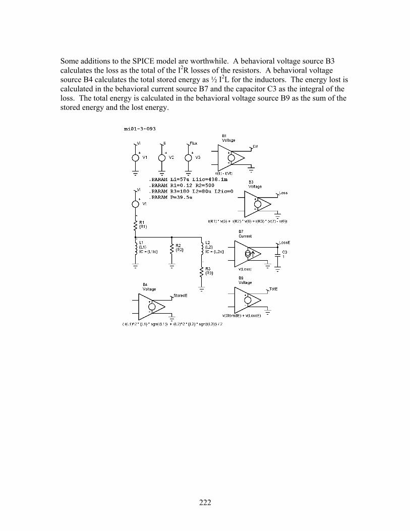
222

Some additions to the SPICE model are worthwhile. A behavioral voltage source B3 calculates the loss as the total of the I2R losses of the resistors. A behavioral voltage source B4 calculates the total stored energy as ½ I2L for the inductors. The energy lost is calculated in the behavioral current source B7 and the capacitor C3 as the integral of the loss. The total energy is calculated in the behavioral voltage source B9 as the sum of the stored energy and the lost energy.

223

The picture below shows the input voltage Vi and the loss. Note that this is not the same as the Pi shown on the Excel Tool–it is the loss calculated in the model resistances. The loss never goes to zero and persists after the voltage is removed.

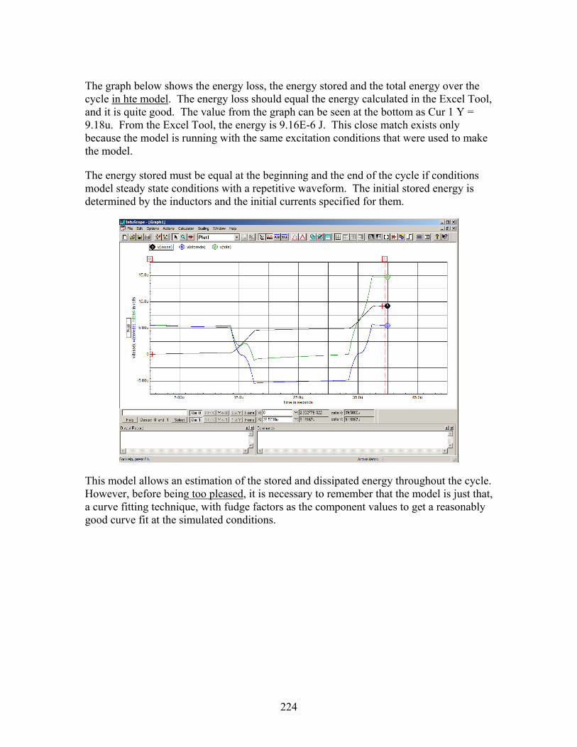
224

The graph below shows the energy loss, the energy stored and the total energy over the cycle in hte model. The energy loss should equal the energy calculated in the Excel Tool, and it is quite good. The value from the graph can be seen at the bottom as Cur 1 Y = 9.18u. From the Excel Tool, the energy is 9.16E-6 J. This close match exists only because the model is running with the same excitation conditions that were used to make the model.

The energy stored must be equal at the beginning and the end of the cycle if conditions model steady state conditions with a repetitive waveform. The initial stored energy is determined by the inductors and the initial currents specified for them.

This model allows an estimation of the stored and dissipated energy throughout the cycle. However, before being too pleased, it is necessary to remember that the model is just that, a curve fitting technique, with fudge factors as the component values to get a reasonably good curve fit at the simulated conditions.

225

Using the model with other waveforms

Ideally, the model would accurately predict the current with other excitation levels and waveforms.

To compare the model using other waveforms, the Excel Tool is updated with the .csv data of the new waveform. This immediately updates the files in the SPICE model as well. However, the period P and the initial currents L1ic and L2ic have to be set for the new curve. The data selected is mi01-3-156, a "Hippo curve" with an off-time of 15.8 µs and Vi of 12.5 V. The graph below is copied and pasted from the Excel Tool.

mi01-3-156

Input Voltagei

-15.00

-10.00

-5.00

0.00

5.00

10.00

15.00

0.0E+00 5.0E-06 1.0E-05 1.5E-05 2.0E-05 2.5E-05 3.0E-05 3.5E-05 4.0E-05 4.5E-05

Time

Vi

226

The input current v(Ii) from the .csv data and the model current i(Vt) are shown with the Dif error current. The errors are significant.

227

The hysteresis curve for the model vs the data is shown below. The blue hysteresis loop is from the SPICE model and the black hysteresis loop is using the .csv data input current, both with the .csv input flux as the vertical axis. By taking the ratio of the areas inside the hysteresis loops, we find that the model estimates the loss about 12 percent low.

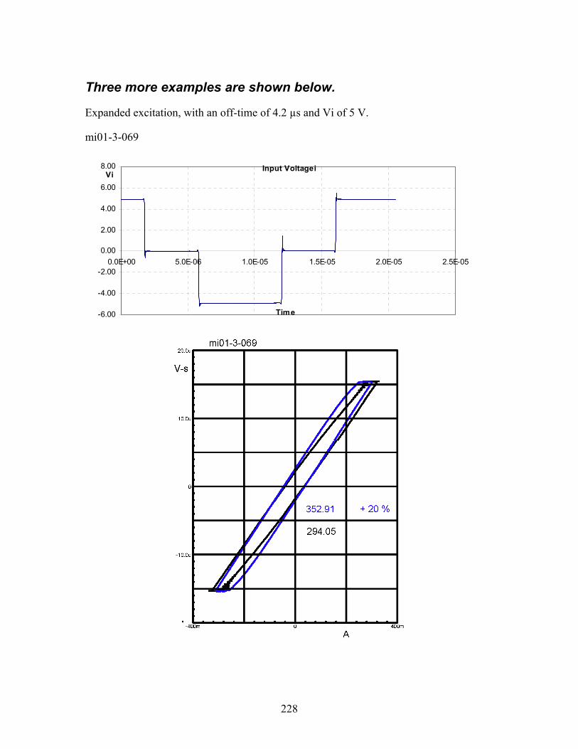
228

Three more examples are shown below.

Expanded excitation, with an off-time of 4.2 µs and Vi of 5 V.

mi01-3-069

Input Voltagei

-6.00

-4.00

-2.00

0.00

2.00

4.00

6.00

8.00

0.0E+00 5.0E-06 1.0E-05 1.5E-05 2.0E-05 2.5E-05

Time

Vi

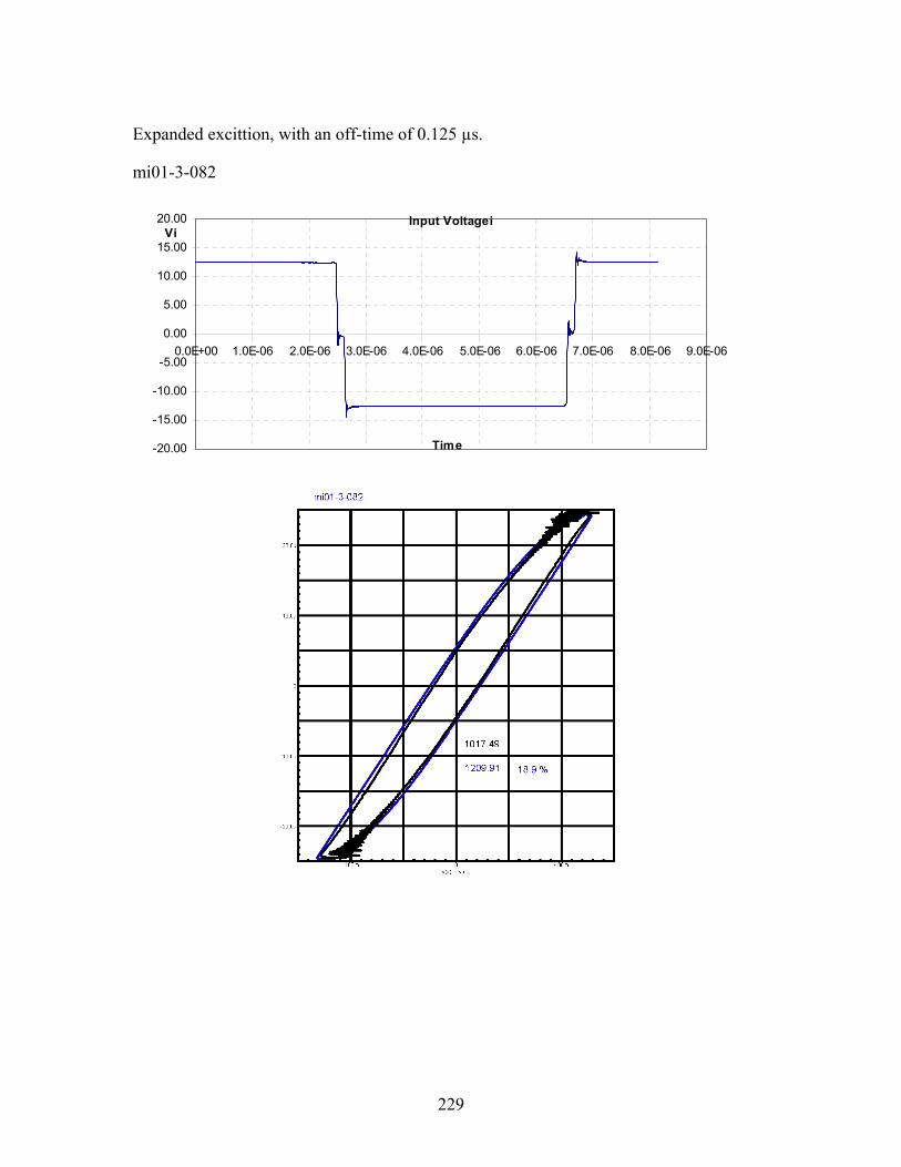
229

Expanded excittion, with an off-time of 0.125 µs.

mi01-3-082

Input Voltagei

-20.00

-15.00

-10.00

-5.00

0.00

5.00

10.00

15.00

20.00

0.0E+00 1.0E-06 2.0E-06 3.0E-06 4.0E-06 5.0E-06 6.0E-06 7.0E-06 8.0E-06 9.0E-06

Time

Vi

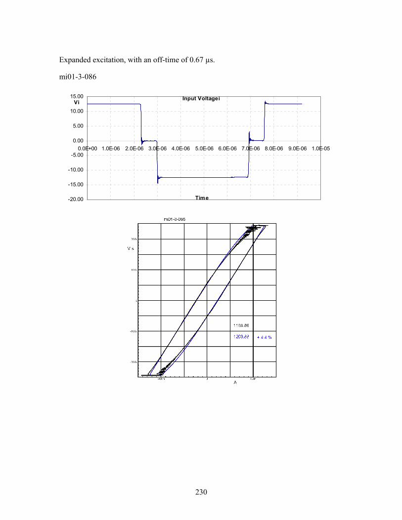
230

Expanded excitation, with an off-time of 0.67 µs.

mi01-3-086

Input Voltagei

-20.00

-15.00

-10.00

-5.00

0.00

5.00

10.00

15.00

0.0E+00 1.0E-06 2.0E-06 3.0E-06 4.0E-06 5.0E-06 6.0E-06 7.0E-06 8.0E-06 9.0E-06 1.0E-05

Time

Vi

231

References [1] User-friendly Data for Magnetic Core Loss Calculations, Edward Herbert, Canton, CT. November 10, 2008. This document is in Appendix A, and can be downloaded from http://www.psma.com/coreloss/eh1.pdf

[2] Improved Core Loss Calculation for Magnetic Components Employed in Power Electronic Systems, APEC 2011, J. Mühlethaler*, J. Bielay†, J. W. Kolar*, and A. Ecklebez‡, *Power Electronic Systems Laboratory, ETH Zurich, †Laboratory for High Power Electronic Systems, ETH Zurich, ‡ABB Switzerland Ltd., Corporate Research, Baden-Dättwil, Switzerland.

[3] Dr. Sullivan presented a paper at APEC2010, Core Loss Predictions for General PWM Waveforms from a Simplified Set of Measured Data

Patent status

This technology may be covered by patents or patents pending.