2/12/2014

1

Unit 2Statistics of One Variable

Displaying Quantitative Data

Displaying Quantitative Data

Today we are going to analyse the following data sets:

Final Grade30.030.036.540.243.749.850.652.151.854.0

…

Set I:

This data set contains the final marks of all 77 students taught by Mr. D in a semester.

For this example the primary data Final Grade represents a quantitative continuous variable.

2/12/2014

2

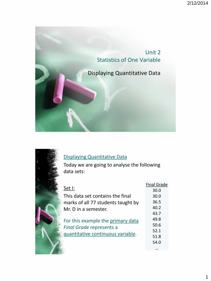
Set II:

This data set shows the 100 NHL players with the highest number of points as of February 11, 2014. Points are the total number of goals and assists a player has. Player Points

Sidney Crosby 78Ryan Getzlaf 67John Tavares 66Phil Kessel 65Patrick Kane 63Alex Ovechkin 60Corey Perry 60Kyle Okposo 59Patrick Sharp 58… …

For this example the secondary data is classified as quantitative and discrete

http://www.nhl.com/ice/playerstats.htm

What should you do with data sets such as these?

Make a Picture• A display of your data will reveal things you

are not likely to see in a list of numbers.

Note• Since few of the data points occur more

than once, a frequency table for each data value would not be very useful.

2/12/2014

3

• To make the data more meaningful, we group the data into equal width piles called bins.

Bin containing all the students with a rounded mark of 73%

Bin containing all the students with a mark between 70% and 80%

How many intervals (bins) do you need?

• There should be between 6 and 10 intervals

•All of the intervals should be the same length (called the bin width)

• There should be no gaps between the intervals

• The data should not be able to be placed on an interval boundary

In some cases you may be able to determine a suitable bin width (i.e. grades; bin width = 10) In other scenarios you could use the following formula to help determine a suitable bin width:

Bin Width =Max Value − Min Value

Number of Bins

2/12/2014

4

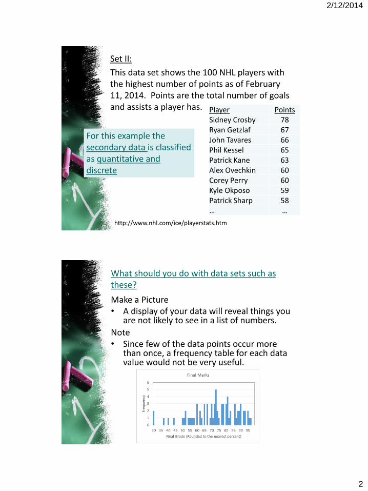
For the NHL data given in set II, the points each player has represents discrete data.

Quantitative Discrete Data

Without placing the data into bins we have the following graph:

For the points data we have a maximum value of 78 and minimum of 35 points.

Bin Width =Max Value − Min Value

Number of Bins=78 − 35

8

= 5.375

So a bin width of 5 or 6 would be reasonable however 5 is a nice number for our data.

To better display the data we need to determine a suitable bin width.

2/12/2014

5

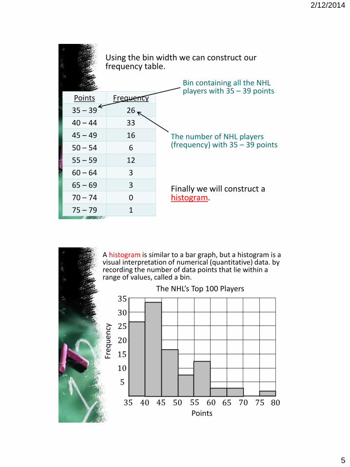
Points Frequency

35 – 39 26

40 – 44 33

45 – 49 16

50 – 54 6

55 – 59 12

60 – 64 3

65 – 69 3

70 – 74 0

75 – 79 1

Bin containing all the NHL players with 35 – 39 points

The number of NHL players (frequency) with 35 – 39 points

Finally we will construct a histogram.

Using the bin width we can construct our frequency table.

35 40 70 7545 50 55 60 65 80

5

10

15

20

25

30

35

Points

Freq

ue

ncy

The NHL’s Top 100 Players

A histogram is similar to a bar graph, but a histogram is a visual interpretation of numerical (quantitative) data. by recording the number of data points that lie within a range of values, called a bin.

2/12/2014

6

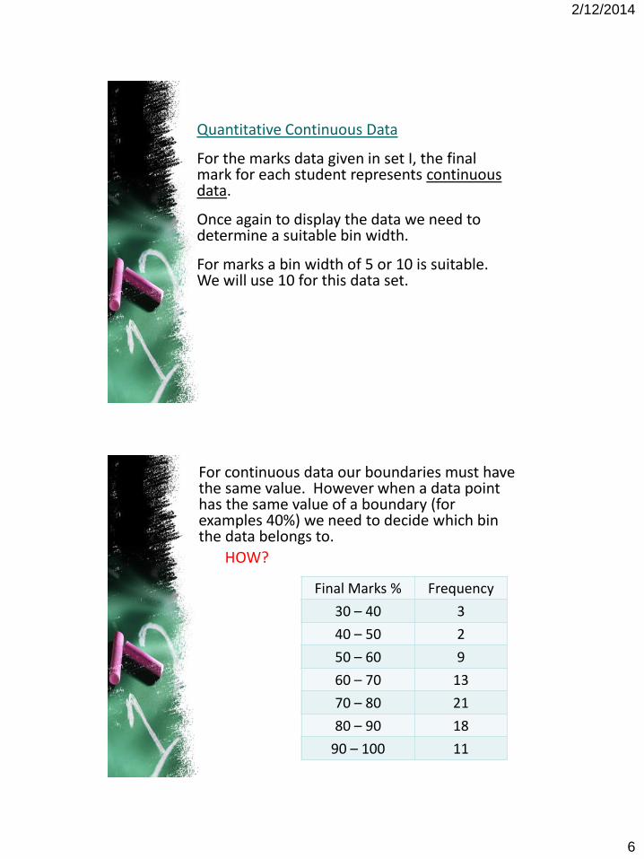
Quantitative Continuous Data

For the marks data given in set I, the final mark for each student represents continuous data.

For marks a bin width of 5 or 10 is suitable. We will use 10 for this data set.

Once again to display the data we need to determine a suitable bin width.

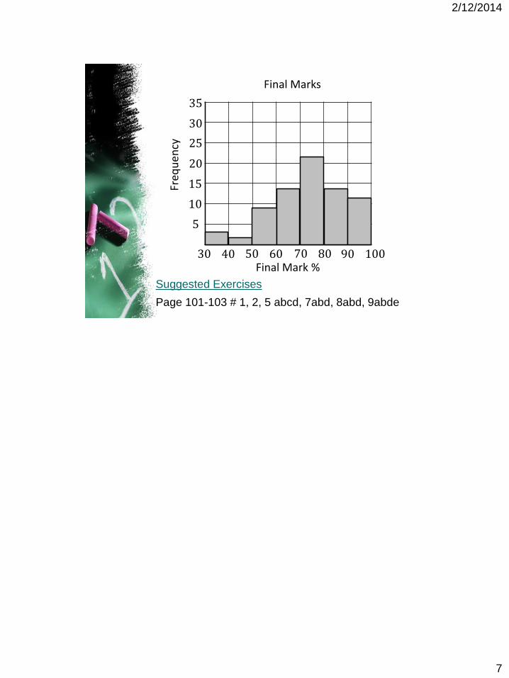
Final Marks % Final Marks % Frequency

30.0 – 39.9 30 – 40 3

40.0 – 49.9 40 – 50 2

50.0 – 59.9 50 – 60 9

60.0 – 69.9 60 – 70 13

70.0 – 79.9 70 – 80 21

80.0 – 89.9 80 – 90 18

90.0 – 99.9 90 – 100 11

For continuous data our boundaries must have the same value. However when a data point has the same value of a boundary (for examples 40%) we need to decide which bin the data belongs to.

HOW?

2/12/2014

7

Suggested Exercises

Page 101-103 # 1, 2, 5 abcd, 7abd, 8abd, 9abde

30 40 10050 60 70 80 90

5

10

15

20

25

30

35

Final Mark %

Freq

ue

ncy

Final Marks