Unfolding the IBM eServer Blue Gene Solution · Eserver Blue Gene Solution Nicholas Allsopp Antoine Tabary Jonathan Follows Pascal Vezolle Michael Hennecke Hari Reddy Fumiyasu Ishibashi

ibm.com/redbooks

Unfolding the IBM Eserver Blue Gene Solution

Nicholas Allsopp Antoine TabaryJonathan Follows Pascal VezolleMichael Hennecke Hari ReddyFumiyasu Ishibashi Carlos SosaMichael Paolini Sheeba PrakashDino Quintero Octavian Lascu

Understand the Blue Gene architecture

Select suitable applications for implementation

Learn about our experiences in porting parallel applications

Front cover

http://www.redbooks.ibm.com/


Unfolding the IBM Eserver Blue Gene Solution

September 2005

International Technical Support Organization

SG24-6686-00

© Copyright International Business Machines Corporation 2005. All rights reserved.Note to U.S. Government Users Restricted Rights -- Use, duplication or disclosure restricted by GSA ADPSchedule Contract with IBM Corp.

First Edition (September 2005)

This edition applies to IBM eServer Blue Gene Solution Driver Version 280 (July 8th, 2005).

Note: Before using this information and the product it supports, read the information in “Notices” on page xi.

Contents

Notices . . . . . . . . . . . . . . . . . . . . . . . . . . . . . . . . . . . . . . . . . . . . . . . . . . . . . . . xiTrademarks . . . . . . . . . . . . . . . . . . . . . . . . . . . . . . . . . . . . . . . . . . . . . . . . . . . xii

Preface . . . . . . . . . . . . . . . . . . . . . . . . . . . . . . . . . . . . . . . . . . . . . . . . . . . . . . xiiiThe team that wrote this redbook. . . . . . . . . . . . . . . . . . . . . . . . . . . . . . . . . . . xiiiBecome a published author . . . . . . . . . . . . . . . . . . . . . . . . . . . . . . . . . . . . . . . xviComments welcome. . . . . . . . . . . . . . . . . . . . . . . . . . . . . . . . . . . . . . . . . . . . xvii

Part 1. Blue Gene/L - the System. . . . . . . . . . . . . . . . . . . . . . . . . . . . . . . . . . . . . . . . . . . . . . . 1

Chapter 1. Introduction to BG/L . . . . . . . . . . . . . . . . . . . . . . . . . . . . . . . . . . . 31.1 Overview of massive parallel processing (MPP) . . . . . . . . . . . . . . . . . . . . . 41.2 Overview of the IBM eServer Blue Gene Solution . . . . . . . . . . . . . . . . . . . 7

1.2.1 Blue Gene/L design points . . . . . . . . . . . . . . . . . . . . . . . . . . . . . . . . . 81.2.2 Where does BlueGene/L fit into the picture . . . . . . . . . . . . . . . . . . . 11

Chapter 2. Blue Gene/L architecture . . . . . . . . . . . . . . . . . . . . . . . . . . . . . . 132.1 General architecture . . . . . . . . . . . . . . . . . . . . . . . . . . . . . . . . . . . . . . . . . 14

2.1.1 Nodes (Compute, I/O) . . . . . . . . . . . . . . . . . . . . . . . . . . . . . . . . . . . . 162.1.2 Blue Gene/L environment . . . . . . . . . . . . . . . . . . . . . . . . . . . . . . . . . 162.1.3 The service node (one per Blue Gene/L system) . . . . . . . . . . . . . . . 182.1.4 One or more front-end nodes . . . . . . . . . . . . . . . . . . . . . . . . . . . . . . 182.1.5 File system . . . . . . . . . . . . . . . . . . . . . . . . . . . . . . . . . . . . . . . . . . . . 182.1.6 Communications . . . . . . . . . . . . . . . . . . . . . . . . . . . . . . . . . . . . . . . . 192.1.7 Execution environment . . . . . . . . . . . . . . . . . . . . . . . . . . . . . . . . . . . 242.1.8 Handling failures . . . . . . . . . . . . . . . . . . . . . . . . . . . . . . . . . . . . . . . . 26

2.2 Node hardware . . . . . . . . . . . . . . . . . . . . . . . . . . . . . . . . . . . . . . . . . . . . . 272.2.1 Processor – System-on-a-chip – the PPC440 . . . . . . . . . . . . . . . . . 272.2.2 Blue Gene/L PowerPC 440 core overview . . . . . . . . . . . . . . . . . . . . 292.2.3 Memory system overview . . . . . . . . . . . . . . . . . . . . . . . . . . . . . . . . . 312.2.4 Double floating point unit overview . . . . . . . . . . . . . . . . . . . . . . . . . . 33

2.3 Blue Gene/L Software . . . . . . . . . . . . . . . . . . . . . . . . . . . . . . . . . . . . . . . . 352.3.1 System software . . . . . . . . . . . . . . . . . . . . . . . . . . . . . . . . . . . . . . . . 352.3.2 Management software. . . . . . . . . . . . . . . . . . . . . . . . . . . . . . . . . . . . 36

Chapter 3. Planning and sizing guidelines . . . . . . . . . . . . . . . . . . . . . . . . . 393.1 Introduction to Blue Gene/L architecture. . . . . . . . . . . . . . . . . . . . . . . . . . 40

3.1.1 Compute nodes and I/O nodes . . . . . . . . . . . . . . . . . . . . . . . . . . . . . 403.1.2 Compute node to I/O node ratio . . . . . . . . . . . . . . . . . . . . . . . . . . . . 42

© Copyright IBM Corp. 2005. All rights reserved. iii

3.1.3 Building blocks for scalable I/O . . . . . . . . . . . . . . . . . . . . . . . . . . . . . 443.2 Service node and front end nodes . . . . . . . . . . . . . . . . . . . . . . . . . . . . . . 45

3.2.1 Hardware planning . . . . . . . . . . . . . . . . . . . . . . . . . . . . . . . . . . . . . . 463.2.2 Operating system . . . . . . . . . . . . . . . . . . . . . . . . . . . . . . . . . . . . . . . 503.2.3 Software . . . . . . . . . . . . . . . . . . . . . . . . . . . . . . . . . . . . . . . . . . . . . . 51

3.3 Network sizing considerations. . . . . . . . . . . . . . . . . . . . . . . . . . . . . . . . . . 533.3.1 Functional network . . . . . . . . . . . . . . . . . . . . . . . . . . . . . . . . . . . . . . 533.3.2 Control (service) network . . . . . . . . . . . . . . . . . . . . . . . . . . . . . . . . . 54

3.4 File system configuration. . . . . . . . . . . . . . . . . . . . . . . . . . . . . . . . . . . . . . 563.4.1 I/O servers. . . . . . . . . . . . . . . . . . . . . . . . . . . . . . . . . . . . . . . . . . . . . 573.4.2 NFS . . . . . . . . . . . . . . . . . . . . . . . . . . . . . . . . . . . . . . . . . . . . . . . . . . 583.4.3 GPFS . . . . . . . . . . . . . . . . . . . . . . . . . . . . . . . . . . . . . . . . . . . . . . . . 60

Chapter 4. System management . . . . . . . . . . . . . . . . . . . . . . . . . . . . . . . . . 634.1 Operating your BG/L . . . . . . . . . . . . . . . . . . . . . . . . . . . . . . . . . . . . . . . . . 64

4.1.1 Remote shell . . . . . . . . . . . . . . . . . . . . . . . . . . . . . . . . . . . . . . . . . . . 644.2 Monitoring (HW, system SW) . . . . . . . . . . . . . . . . . . . . . . . . . . . . . . . . . . 66

4.2.1 Monitoring logs via the MMCS software . . . . . . . . . . . . . . . . . . . . . . 664.2.2 Monitoring via the databases . . . . . . . . . . . . . . . . . . . . . . . . . . . . . . 674.2.3 Web interface for the database (BGWEB) . . . . . . . . . . . . . . . . . . . . 70

4.3 User environment (variables, directories) . . . . . . . . . . . . . . . . . . . . . . . . . 754.3.1 Variables for DB2 . . . . . . . . . . . . . . . . . . . . . . . . . . . . . . . . . . . . . . . 764.3.2 Variables for MMCS . . . . . . . . . . . . . . . . . . . . . . . . . . . . . . . . . . . . . 764.3.3 Variables for MPIRUN. . . . . . . . . . . . . . . . . . . . . . . . . . . . . . . . . . . . 764.3.4 Variables for the compilers . . . . . . . . . . . . . . . . . . . . . . . . . . . . . . . . 774.3.5 The /bgl directory (the shared file system) . . . . . . . . . . . . . . . . . . . . 77

4.4 Scheduling (running) jobs . . . . . . . . . . . . . . . . . . . . . . . . . . . . . . . . . . . . . 774.4.1 MPIRUN . . . . . . . . . . . . . . . . . . . . . . . . . . . . . . . . . . . . . . . . . . . . . . 784.4.2 IBM LoadLeveler . . . . . . . . . . . . . . . . . . . . . . . . . . . . . . . . . . . . . . . . 784.4.3 mmcs_db_console . . . . . . . . . . . . . . . . . . . . . . . . . . . . . . . . . . . . . . 78

4.5 Configuration and reconfiguration . . . . . . . . . . . . . . . . . . . . . . . . . . . . . . . 794.5.1 Configuring system software images . . . . . . . . . . . . . . . . . . . . . . . . 794.5.2 Blocks (Partitions) . . . . . . . . . . . . . . . . . . . . . . . . . . . . . . . . . . . . . . . 79

Part 2. BG/L application environment . . . . . . . . . . . . . . . . . . . . . . . . . . . . . . . . . . . . . . . . . . 81

Chapter 5. Parallel environment. . . . . . . . . . . . . . . . . . . . . . . . . . . . . . . . . . 835.1 Application development environment . . . . . . . . . . . . . . . . . . . . . . . . . . . 845.2 XL compilers . . . . . . . . . . . . . . . . . . . . . . . . . . . . . . . . . . . . . . . . . . . . . . . 86

5.2.1 Optimization level . . . . . . . . . . . . . . . . . . . . . . . . . . . . . . . . . . . . . . . 865.2.2 Machine-specific flags. . . . . . . . . . . . . . . . . . . . . . . . . . . . . . . . . . . . 885.2.3 High-order transformations . . . . . . . . . . . . . . . . . . . . . . . . . . . . . . . . 895.2.4 Interprocedural analysis . . . . . . . . . . . . . . . . . . . . . . . . . . . . . . . . . . 905.2.5 XL FORTRAN new and changed functionality . . . . . . . . . . . . . . . . . 90

iv Unfolding the IBM ̂Blue Gene Solution

5.2.6 Compiler directives for performance . . . . . . . . . . . . . . . . . . . . . . . . . 925.2.7 Directive usage . . . . . . . . . . . . . . . . . . . . . . . . . . . . . . . . . . . . . . . . . 945.2.8 Blue Gene/L compiler features . . . . . . . . . . . . . . . . . . . . . . . . . . . . . 965.2.9 Blue Gene/L compiler flags . . . . . . . . . . . . . . . . . . . . . . . . . . . . . . . 101

5.3 Parallel execution environment . . . . . . . . . . . . . . . . . . . . . . . . . . . . . . . . 1025.3.1 Using mpirun . . . . . . . . . . . . . . . . . . . . . . . . . . . . . . . . . . . . . . . . . . 1075.3.2 Mapping MPI tasks to Blue Gene/L nodes . . . . . . . . . . . . . . . . . . . 109

5.4 Other application development tools . . . . . . . . . . . . . . . . . . . . . . . . . . . . 1175.4.1 The environment on the front-end nodes . . . . . . . . . . . . . . . . . . . . 1175.4.2 Debuggers. . . . . . . . . . . . . . . . . . . . . . . . . . . . . . . . . . . . . . . . . . . . 1175.4.3 Profiling . . . . . . . . . . . . . . . . . . . . . . . . . . . . . . . . . . . . . . . . . . . . . . 1185.4.4 BG/L hardware counters . . . . . . . . . . . . . . . . . . . . . . . . . . . . . . . . . 1185.4.5 The IBM High Performance Computing Toolkit. . . . . . . . . . . . . . . . 1195.4.6 Third-party performance tools . . . . . . . . . . . . . . . . . . . . . . . . . . . . . 122

5.5 Job management. . . . . . . . . . . . . . . . . . . . . . . . . . . . . . . . . . . . . . . . . . . 1235.5.1 LoadLeveler . . . . . . . . . . . . . . . . . . . . . . . . . . . . . . . . . . . . . . . . . . 123

Chapter 6. Porting applications . . . . . . . . . . . . . . . . . . . . . . . . . . . . . . . . . 1276.1 Does your application fit on Blue Gene/L . . . . . . . . . . . . . . . . . . . . . . . . 128

6.1.1 System call summary . . . . . . . . . . . . . . . . . . . . . . . . . . . . . . . . . . . 1286.1.2 Processes and threads . . . . . . . . . . . . . . . . . . . . . . . . . . . . . . . . . . 1296.1.3 File system calls . . . . . . . . . . . . . . . . . . . . . . . . . . . . . . . . . . . . . . . 1316.1.4 I/O-intensive applications . . . . . . . . . . . . . . . . . . . . . . . . . . . . . . . . 1326.1.5 Networking support . . . . . . . . . . . . . . . . . . . . . . . . . . . . . . . . . . . . . 1336.1.6 Timer support . . . . . . . . . . . . . . . . . . . . . . . . . . . . . . . . . . . . . . . . . 1336.1.7 STDIN support . . . . . . . . . . . . . . . . . . . . . . . . . . . . . . . . . . . . . . . . 1346.1.8 Memory . . . . . . . . . . . . . . . . . . . . . . . . . . . . . . . . . . . . . . . . . . . . . . 1346.1.9 SMP . . . . . . . . . . . . . . . . . . . . . . . . . . . . . . . . . . . . . . . . . . . . . . . . 136

6.2 Single CPU - porting serial applications . . . . . . . . . . . . . . . . . . . . . . . . . 1376.2.1 Porting serial code on Blue Gene/L . . . . . . . . . . . . . . . . . . . . . . . . 1386.2.2 Obtaining and understanding an object code listing . . . . . . . . . . . . 1426.2.3 Memory alignment, aliasing, and versioning . . . . . . . . . . . . . . . . . . 1466.2.4 Exploiting the double FPU. . . . . . . . . . . . . . . . . . . . . . . . . . . . . . . . 1506.2.5 Divide, square root operations, and vector intrinsic functions. . . . . 1596.2.6 Memory management . . . . . . . . . . . . . . . . . . . . . . . . . . . . . . . . . . . 1606.2.7 Math libraries. . . . . . . . . . . . . . . . . . . . . . . . . . . . . . . . . . . . . . . . . . 1686.2.8 Performance measurement. . . . . . . . . . . . . . . . . . . . . . . . . . . . . . . 174

6.3 Porting parallel applications . . . . . . . . . . . . . . . . . . . . . . . . . . . . . . . . . . 1766.3.1 The BG/L programming model . . . . . . . . . . . . . . . . . . . . . . . . . . . . 1766.3.2 MPI features supported on BG/L. . . . . . . . . . . . . . . . . . . . . . . . . . . 1776.3.3 The BG/L MPI implementation . . . . . . . . . . . . . . . . . . . . . . . . . . . . 1786.3.4 MPI point-to-point performance. . . . . . . . . . . . . . . . . . . . . . . . . . . . 1846.3.5 MPI collective performance. . . . . . . . . . . . . . . . . . . . . . . . . . . . . . . 188

Contents v

6.3.6 Co-processor mode versus virtual node mode . . . . . . . . . . . . . . . . 1906.4 I/O operations . . . . . . . . . . . . . . . . . . . . . . . . . . . . . . . . . . . . . . . . . . . . . 191

6.4.1 How the I/O works. . . . . . . . . . . . . . . . . . . . . . . . . . . . . . . . . . . . . . 1916.4.2 Compute nodes mapping to I/O nodes . . . . . . . . . . . . . . . . . . . . . . 1936.4.3 Do not use one file per I/O node . . . . . . . . . . . . . . . . . . . . . . . . . . . 1956.4.4 Do not use one task doing all I/O . . . . . . . . . . . . . . . . . . . . . . . . . . 195

6.5 Debugging . . . . . . . . . . . . . . . . . . . . . . . . . . . . . . . . . . . . . . . . . . . . . . . . 1966.5.1 Debugging by printf() or PRINT. . . . . . . . . . . . . . . . . . . . . . . . . . . . 1966.5.2 Instrumenting function entry and exit . . . . . . . . . . . . . . . . . . . . . . . 1966.5.3 Using the GNU debugger . . . . . . . . . . . . . . . . . . . . . . . . . . . . . . . . 1986.5.4 TotalView . . . . . . . . . . . . . . . . . . . . . . . . . . . . . . . . . . . . . . . . . . . . 2046.5.5 Debugging parallel programs . . . . . . . . . . . . . . . . . . . . . . . . . . . . . 2056.5.6 Tracking your memory usage . . . . . . . . . . . . . . . . . . . . . . . . . . . . . 2056.5.7 Core files and addr2line . . . . . . . . . . . . . . . . . . . . . . . . . . . . . . . . . 205

Chapter 7. Massively parallel tuning . . . . . . . . . . . . . . . . . . . . . . . . . . . . . 2077.1 Application mapping . . . . . . . . . . . . . . . . . . . . . . . . . . . . . . . . . . . . . . . . 208

7.1.1 Problem description . . . . . . . . . . . . . . . . . . . . . . . . . . . . . . . . . . . . 2087.1.2 Mapping scenarios . . . . . . . . . . . . . . . . . . . . . . . . . . . . . . . . . . . . . 2117.1.3 Mapping file semantics in Blue Gene/L. . . . . . . . . . . . . . . . . . . . . . 2177.1.4 Automatic mapping methods. . . . . . . . . . . . . . . . . . . . . . . . . . . . . . 2207.1.5 Manual mapping methods. . . . . . . . . . . . . . . . . . . . . . . . . . . . . . . . 2237.1.6 Mapping experiments . . . . . . . . . . . . . . . . . . . . . . . . . . . . . . . . . . . 2267.1.7 General guidelines for application mapping . . . . . . . . . . . . . . . . . . 2307.1.8 MPI topologies and Cartesian communicators . . . . . . . . . . . . . . . . 231

7.2 Limitations on scaling . . . . . . . . . . . . . . . . . . . . . . . . . . . . . . . . . . . . . . . 2387.3 Hints on how to parallelize codes . . . . . . . . . . . . . . . . . . . . . . . . . . . . . . 239

7.3.1 All-to-all communication . . . . . . . . . . . . . . . . . . . . . . . . . . . . . . . . . 2397.3.2 Eager limit and message routing. . . . . . . . . . . . . . . . . . . . . . . . . . . 241

7.4 Other general suggestions . . . . . . . . . . . . . . . . . . . . . . . . . . . . . . . . . . . 242

Part 3. Application porting examples . . . . . . . . . . . . . . . . . . . . . . . . . . . . . . . . . . . . . . . . . 247

Chapter 8. Applications on Blue Gene . . . . . . . . . . . . . . . . . . . . . . . . . . . 2498.1 Introduction . . . . . . . . . . . . . . . . . . . . . . . . . . . . . . . . . . . . . . . . . . . . . . . 250

8.1.1 General considerations and benchmark applications . . . . . . . . . . . 2508.1.2 High Performance Linpack (HPL) . . . . . . . . . . . . . . . . . . . . . . . . . . 2508.1.3 NAS Parallel Benchmarks. . . . . . . . . . . . . . . . . . . . . . . . . . . . . . . . 2538.1.4 Intel MPI Benchmarks . . . . . . . . . . . . . . . . . . . . . . . . . . . . . . . . . . . 258

8.2 DL_POLY . . . . . . . . . . . . . . . . . . . . . . . . . . . . . . . . . . . . . . . . . . . . . . . . 2628.2.1 Application description . . . . . . . . . . . . . . . . . . . . . . . . . . . . . . . . . . 2628.2.2 Planning for the application. . . . . . . . . . . . . . . . . . . . . . . . . . . . . . . 2638.2.3 Characteristics of execution . . . . . . . . . . . . . . . . . . . . . . . . . . . . . . 2648.2.4 Scaling and tuning (optimization) . . . . . . . . . . . . . . . . . . . . . . . . . . 265

vi Unfolding the IBM ̂Blue Gene Solution

8.3 AMBER8 . . . . . . . . . . . . . . . . . . . . . . . . . . . . . . . . . . . . . . . . . . . . . . . . . 2688.3.1 AMBER8 description . . . . . . . . . . . . . . . . . . . . . . . . . . . . . . . . . . . . 2688.3.2 AMBER8 characteristics . . . . . . . . . . . . . . . . . . . . . . . . . . . . . . . . . 2708.3.3 Planning for AMBER8 . . . . . . . . . . . . . . . . . . . . . . . . . . . . . . . . . . . 2708.3.4 Blue Gene/L features . . . . . . . . . . . . . . . . . . . . . . . . . . . . . . . . . . . 2718.3.5 Scaling and tuning AMBER8. . . . . . . . . . . . . . . . . . . . . . . . . . . . . . 271

8.4 AVBP. . . . . . . . . . . . . . . . . . . . . . . . . . . . . . . . . . . . . . . . . . . . . . . . . . . . 2778.4.1 Application description . . . . . . . . . . . . . . . . . . . . . . . . . . . . . . . . . . 2778.4.2 Planning for the application. . . . . . . . . . . . . . . . . . . . . . . . . . . . . . . 2808.4.3 Porting experience . . . . . . . . . . . . . . . . . . . . . . . . . . . . . . . . . . . . . 2808.4.4 Scaling and tuning. . . . . . . . . . . . . . . . . . . . . . . . . . . . . . . . . . . . . . 280

8.5 LS-DYNA. . . . . . . . . . . . . . . . . . . . . . . . . . . . . . . . . . . . . . . . . . . . . . . . . 2858.5.1 Introduction . . . . . . . . . . . . . . . . . . . . . . . . . . . . . . . . . . . . . . . . . . . 2858.5.2 Parallel implementation of LS-DYNA . . . . . . . . . . . . . . . . . . . . . . . 2858.5.3 Running LS-DYNA on BG/L . . . . . . . . . . . . . . . . . . . . . . . . . . . . . . 2868.5.4 Scalability results for LS-DYNA on Blue Gene/L. . . . . . . . . . . . . . . 287

8.6 TRACE . . . . . . . . . . . . . . . . . . . . . . . . . . . . . . . . . . . . . . . . . . . . . . . . . . 2918.6.1 Application description . . . . . . . . . . . . . . . . . . . . . . . . . . . . . . . . . . 2918.6.2 Planning for the application. . . . . . . . . . . . . . . . . . . . . . . . . . . . . . . 2918.6.3 Porting experience . . . . . . . . . . . . . . . . . . . . . . . . . . . . . . . . . . . . . 292

8.7 CPMD . . . . . . . . . . . . . . . . . . . . . . . . . . . . . . . . . . . . . . . . . . . . . . . . . . . 2998.7.1 CPMD description . . . . . . . . . . . . . . . . . . . . . . . . . . . . . . . . . . . . . . 2998.7.2 Application characterization . . . . . . . . . . . . . . . . . . . . . . . . . . . . . . 3028.7.3 Enablement experience and test results . . . . . . . . . . . . . . . . . . . . . 3038.7.4 Benchmark Data . . . . . . . . . . . . . . . . . . . . . . . . . . . . . . . . . . . . . . . 303

8.8 WRF . . . . . . . . . . . . . . . . . . . . . . . . . . . . . . . . . . . . . . . . . . . . . . . . . . . . 3068.8.1 Application description . . . . . . . . . . . . . . . . . . . . . . . . . . . . . . . . . . 3068.8.2 Characteristics . . . . . . . . . . . . . . . . . . . . . . . . . . . . . . . . . . . . . . . . 3078.8.3 Planning for the application. . . . . . . . . . . . . . . . . . . . . . . . . . . . . . . 3078.8.4 Porting experience (depending on licensing) . . . . . . . . . . . . . . . . . 3088.8.5 Scaling and tuning (optimization) . . . . . . . . . . . . . . . . . . . . . . . . . . 310

8.9 Local Model . . . . . . . . . . . . . . . . . . . . . . . . . . . . . . . . . . . . . . . . . . . . . . . 3168.9.1 Description . . . . . . . . . . . . . . . . . . . . . . . . . . . . . . . . . . . . . . . . . . . 3168.9.2 Characteristics . . . . . . . . . . . . . . . . . . . . . . . . . . . . . . . . . . . . . . . . 3188.9.3 Planning for LM . . . . . . . . . . . . . . . . . . . . . . . . . . . . . . . . . . . . . . . . 3208.9.4 Porting experience . . . . . . . . . . . . . . . . . . . . . . . . . . . . . . . . . . . . . 3208.9.5 Scaling and tuning. . . . . . . . . . . . . . . . . . . . . . . . . . . . . . . . . . . . . . 322

Part 4. Appendixes . . . . . . . . . . . . . . . . . . . . . . . . . . . . . . . . . . . . . . . . . . . . . . . . . . . . . . . . 327

Appendix A. BG/L prior to porting code . . . . . . . . . . . . . . . . . . . . . . . . . . 329

Appendix B. BG/L runtime system calls . . . . . . . . . . . . . . . . . . . . . . . . . . 331B.1 Calls in rts.h . . . . . . . . . . . . . . . . . . . . . . . . . . . . . . . . . . . . . . . . . . . . . . 332

Contents vii

B.2 Personality data in bglpersonality.h . . . . . . . . . . . . . . . . . . . . . . . . . . . . 333B.2.1 The sanity.c example . . . . . . . . . . . . . . . . . . . . . . . . . . . . . . . . . . . 334B.2.2 Accessing the BG/L runtime information from FORTRAN . . . . . . . 336B.2.3 Sanity revisited: sanity.f90 . . . . . . . . . . . . . . . . . . . . . . . . . . . . . . . 339

Appendix C. Floating point instruction set . . . . . . . . . . . . . . . . . . . . . . . . 341C.1 Instruction types specific to BG/L PPC440 . . . . . . . . . . . . . . . . . . . . . . . 342C.2 Additional floating point instructions . . . . . . . . . . . . . . . . . . . . . . . . . . . . 343

C.2.1 Summary . . . . . . . . . . . . . . . . . . . . . . . . . . . . . . . . . . . . . . . . . . . . 343C.2.2 Add instructions . . . . . . . . . . . . . . . . . . . . . . . . . . . . . . . . . . . . . . . 344C.2.3 Estimate instructions . . . . . . . . . . . . . . . . . . . . . . . . . . . . . . . . . . . 344C.2.4 Multiply instructions . . . . . . . . . . . . . . . . . . . . . . . . . . . . . . . . . . . . 345C.2.5 Multiply-add instructions . . . . . . . . . . . . . . . . . . . . . . . . . . . . . . . . . 345C.2.6 Select instruction . . . . . . . . . . . . . . . . . . . . . . . . . . . . . . . . . . . . . . 347C.2.7 Convert and round instructions. . . . . . . . . . . . . . . . . . . . . . . . . . . . 347C.2.8 Compare instruction . . . . . . . . . . . . . . . . . . . . . . . . . . . . . . . . . . . . 347C.2.9 Move instructions . . . . . . . . . . . . . . . . . . . . . . . . . . . . . . . . . . . . . . 347C.2.10 Load/store instructions . . . . . . . . . . . . . . . . . . . . . . . . . . . . . . . . . 348

Appendix D. Some useful utilities . . . . . . . . . . . . . . . . . . . . . . . . . . . . . . . 351Users who have allocated partitions . . . . . . . . . . . . . . . . . . . . . . . . . . . . . 352Active jobs. . . . . . . . . . . . . . . . . . . . . . . . . . . . . . . . . . . . . . . . . . . . . . . . . 352Partitions which are defined . . . . . . . . . . . . . . . . . . . . . . . . . . . . . . . . . . . 354Console environment . . . . . . . . . . . . . . . . . . . . . . . . . . . . . . . . . . . . . . . . 355

Appendix E. Compiler configuration file . . . . . . . . . . . . . . . . . . . . . . . . . . 357Sample compiler options file . . . . . . . . . . . . . . . . . . . . . . . . . . . . . . . . . . . 358

Appendix F. Systems comparison . . . . . . . . . . . . . . . . . . . . . . . . . . . . . . . 365Blue Gene/L and other contemporary architectures . . . . . . . . . . . . . . . . . 365

Appendix G. Hardware counters . . . . . . . . . . . . . . . . . . . . . . . . . . . . . . . . 369G.1 Link with bgl_perfctr library on Blue Gene/L. . . . . . . . . . . . . . . . . . . . . . 370G.2 API details . . . . . . . . . . . . . . . . . . . . . . . . . . . . . . . . . . . . . . . . . . . . . . . 370G.3 Ways of accessing the counters. . . . . . . . . . . . . . . . . . . . . . . . . . . . . . . 375

G.3.1 Counter update and copy-out. . . . . . . . . . . . . . . . . . . . . . . . . . . . . 375G.3.2 Counter update and immediate access . . . . . . . . . . . . . . . . . . . . . 376G.3.3 Counter update and lock . . . . . . . . . . . . . . . . . . . . . . . . . . . . . . . . 376

G.4 Available counter events . . . . . . . . . . . . . . . . . . . . . . . . . . . . . . . . . . . . 376G.5 Correct API usage . . . . . . . . . . . . . . . . . . . . . . . . . . . . . . . . . . . . . . . . . 377

G.5.1 Using the second CPU . . . . . . . . . . . . . . . . . . . . . . . . . . . . . . . . . . 377G.5.2 Counter start, stop, and reset . . . . . . . . . . . . . . . . . . . . . . . . . . . . . 378G.5.3 Locking semantics of bgl_perfctr . . . . . . . . . . . . . . . . . . . . . . . . . . 379

viii Unfolding the IBM ̂Blue Gene Solution

Abbreviations and acronyms . . . . . . . . . . . . . . . . . . . . . . . . . . . . . . . . . . . 381

Related publications . . . . . . . . . . . . . . . . . . . . . . . . . . . . . . . . . . . . . . . . . . 383IBM Redbooks . . . . . . . . . . . . . . . . . . . . . . . . . . . . . . . . . . . . . . . . . . . . . . . . 383Other publications . . . . . . . . . . . . . . . . . . . . . . . . . . . . . . . . . . . . . . . . . . . . . 383Online resources . . . . . . . . . . . . . . . . . . . . . . . . . . . . . . . . . . . . . . . . . . . . . . 384How to get IBM Redbooks . . . . . . . . . . . . . . . . . . . . . . . . . . . . . . . . . . . . . . . 385Help from IBM . . . . . . . . . . . . . . . . . . . . . . . . . . . . . . . . . . . . . . . . . . . . . . . . 385

Index . . . . . . . . . . . . . . . . . . . . . . . . . . . . . . . . . . . . . . . . . . . . . . . . . . . . . . . 387

Contents ix

x Unfolding the IBM ̂Blue Gene Solution

Notices

This information was developed for products and services offered in the U.S.A.

IBM may not offer the products, services, or features discussed in this document in other countries. Consult your local IBM representative for information on the products and services currently available in your area. Any reference to an IBM product, program, or service is not intended to state or imply that only that IBM product, program, or service may be used. Any functionally equivalent product, program, or service that does not infringe any IBM intellectual property right may be used instead. However, it is the user's responsibility to evaluate and verify the operation of any non-IBM product, program, or service.

IBM may have patents or pending patent applications covering subject matter described in this document. The furnishing of this document does not give you any license to these patents. You can send license inquiries, in writing, to: IBM Director of Licensing, IBM Corporation, North Castle Drive Armonk, NY 10504-1785 U.S.A.

The following paragraph does not apply to the United Kingdom or any other country where such provisions are inconsistent with local law: INTERNATIONAL BUSINESS MACHINES CORPORATION PROVIDES THIS PUBLICATION "AS IS" WITHOUT WARRANTY OF ANY KIND, EITHER EXPRESS OR IMPLIED, INCLUDING, BUT NOT LIMITED TO, THE IMPLIED WARRANTIES OF NON-INFRINGEMENT, MERCHANTABILITY OR FITNESS FOR A PARTICULAR PURPOSE. Some states do not allow disclaimer of express or implied warranties in certain transactions, therefore, this statement may not apply to you.

This information could include technical inaccuracies or typographical errors. Changes are periodically made to the information herein; these changes will be incorporated in new editions of the publication. IBM may make improvements and/or changes in the product(s) and/or the program(s) described in this publication at any time without notice.

Any references in this information to non-IBM Web sites are provided for convenience only and do not in any manner serve as an endorsement of those Web sites. The materials at those Web sites are not part of the materials for this IBM product and use of those Web sites is at your own risk.

IBM may use or distribute any of the information you supply in any way it believes appropriate without incurring any obligation to you.

Information concerning non-IBM products was obtained from the suppliers of those products, their published announcements or other publicly available sources. IBM has not tested those products and cannot confirm the accuracy of performance, compatibility or any other claims related to non-IBM products. Questions on the capabilities of non-IBM products should be addressed to the suppliers of those products.

This information contains examples of data and reports used in daily business operations. To illustrate them as completely as possible, the examples include the names of individuals, companies, brands, and products. All of these names are fictitious and any similarity to the names and addresses used by an actual business enterprise is entirely coincidental.

COPYRIGHT LICENSE: This information contains sample application programs in source language, which illustrates programming techniques on various operating platforms. You may copy, modify, and distribute these sample programs in any form without payment to IBM, for the purposes of developing, using, marketing or distributing application programs conforming to the application programming interface for the operating platform for which the sample programs are written. These examples have not been thoroughly tested under all conditions. IBM, therefore, cannot guarantee or imply reliability, serviceability, or function of these programs. You may copy, modify, and distribute these sample programs in any form without payment to IBM for the purposes of developing, using, marketing, or distributing application programs conforming to IBM's application programming interfaces.

© Copyright IBM Corp. 2005. All rights reserved. xi

TrademarksThe following terms are trademarks of the International Business Machines Corporation in the United States, other countries, or both:

Eserver®Eserver®Redbooks (logo) ™eServer™pSeries®xSeries®AIX 5L™AIX®

BladeCenter®Blue Gene®DB2®IBM®LoadLeveler®Open Power™PowerPC®POWER™

POWER3™POWER4™POWER5™Redbooks™Roma®RS/6000®WebSphere®

The following terms are trademarks of other companies:

Java, PDB, Sun, and all Java-based trademarks are trademarks of Sun Microsystems, Inc. in the United States, other countries, or both.

Microsoft, Outlook, Windows, and the Windows logo are trademarks of Microsoft Corporation in the United States, other countries, or both.

Intel, Itanium, Pentium, Intel logo, Intel Inside logo, and Intel Centrino logo are trademarks or registered trademarks of Intel Corporation or its subsidiaries in the United States, other countries, or both.

UNIX is a registered trademark of The Open Group in the United States and other countries.

Linux is a trademark of Linus Torvalds in the United States, other countries, or both.

Other company, product, and service names may be trademarks or service marks of others.

xii Unfolding the IBM ̂Blue Gene Solution

Preface

The IBM® eServer™ Blue Gene® Solution is a commercial version of the research project, and Blue Gene/L represents a new entrant in the IBM Deep Computing Portfolio. This IBM Redbook will help you to design and create a solution for migrating and porting existing applications to run on the IBM eServer Blue Gene system. It is targeted to application designers and programmers working in a High Performance Computing environment.

The book is composed of three parts. In the first part we present an architectural overview of the IBM eServer Blue Gene Solution, and describe the design principles underlying this revolutionary supercomputer.

In the second part we summarize general guidelines for identifying the structure of your application. Because simple application recompilation may not efficiently exploit the massively parallel structure of this system, we identify and classify the application characteristics you need to consider for efficient implementation on the IBM eServer Blue Gene System.

In the final part, we describe several application porting experiences tested during this project. Note that these experiences are presented for reference only, and that the applications were not completely optimized for running on this supercomputer. Nevertheless, they provide valuable insight into what you can expect when running your application on a Blue Gene system.

The team that wrote this redbookThis redbook was produced by a team of specialists from around the world working at the International Technical Support Organization, Poughkeepsie Center.

Octavian Lascu is a Project Leader at the International Technical Support Organization, Poughkeepsie Center. He writes extensively and teaches IBM classes worldwide on all areas of pSeries® and Linux® clusters. Before joining the ITSO, Octavian worked in IBM Global Services Romania as a software and hardware Services Manager. He holds a Master's Degree in Electronic Engineering from the Polytechnical Institute in Bucharest and is also an IBM Certified Advanced Technical Expert in AIX/PSSP/HACMP. He has worked with IBM since 1992.

© Copyright IBM Corp. 2005. All rights reserved. xiii

Dr. Nicholas Allsopp is an IT Specialist in the High Performance Computing and Life Science group within Emerging Technology, Hursley Laboratory, UK. His area of expertise is the porting and tuning of scientific and technical parallel applications onto IBM hardware. He has been working with parallel computers for more than 10 years. He holds a degree in Computer Aided Physics and a Ph.D. in theoretical condensed matter physics.

Dr. Pascal Vezolle is an IBM Certified IT Specialist in the fields of systems products and technical sales support. He works in the EMEA Deep Computing organization at the Product Software Solution Center located in France. He has more than 10 years of experience in high performance computing. Before joining IBM in 2001 he worked for COMPAQ, where he was in charge of ISV support; and for Saint-Gobain, where he was responsible for the Computing Research center.

Jonathan Follows is an IBM Consulting IT Specialist in the UK. He designs and helps implement high performance computing systems. He has 20 years of experience with IBM and is a certified IT Specialist in the fields of networking and large systems. Jonathan spent two years at the ITSO, Raleigh, writing books on networking hardware and software. Jonathan studied Mathematics at Oxford University, England, and holds a degree in Computing Science from London University, England.

Michael Hennecke is an IT Specialist in the Deep Computing team in IBM Germany, and is currently working as EMEA HPC technical architect for the public sector. Before joining IBM, he worked at the Computing Center of the University of Karlsruhe, Germany. Michael has 14 years of experience with parallel computing, including ten years on the RS/6000® SP and Cluster 1600. He holds a degree in Physics from the University of Bochum (RUB), Germany.

Fumiyasu Ishibashi is an IT Specialist in IBM Japan. He has over three years of experience in deploying Linux solutions in complex environments. His areas of expertise include Linux, networking, applications and high performance computing clusters.

Michael Paolini is a Senior Solutions Architect within eServer Solutions for the IBM Systems and Technology Group. He is responsible for driving strategy and creation of Open Standards-based industry solutions architectures. Michael was awarded the title of IBM Master Inventor for his extensive body of work, which includes patents consistently ranked in the top tier of the IBM portfolio. Some of the areas that Michael has worked in include the IBM Retail Environment for SUSE Linux (IRES), WebSphere® Telecom Application Server (WTAS), UDDI (Universal Description, Discovery, and Integration), SVG (Scalable Vector Graphics), Web Services and the IBM WS Toolkit, Special Needs and Accessibility, National Language Support (NLS) and Internationalization (L10 & I18N), Device Drivers, and File Systems.

xiv Unfolding the IBM ̂Blue Gene Solution

Sheeba Prakash is an Advisory Software Engineer with the High Performance Computing Team at IBM. She is an IBM Certified Advisory Accredited IT Specialist in Technical Sales Support for pSeries UNIX® Systems. Sheeba works at the eServer xSeries® and HPC Benchmark Center and provides benchmark support for scientific and technical applications on p and x Series Systems. She holds a Master's degree in Traffic Engineering and Transportation Planning from National Institute of Technology, Calicut, India, and a Master of Science in Computer Science from the University of Houston, Texas.

Dr. Hari Reddy is a Senior Software Engineer in Solution Enablement in the IBM Systems and Technology Group. Hari joined IBM in 1990, and his areas of expertise include porting and tuning large scale parallel applications. Hari has 18 years of experience in parallel computing dating back to Intel®'s Hypercube. He holds Master of Science degrees in Operations Research and Computer Science, and a Ph.D. in Computer Science.

Dr. Carlos Sosa is a Senior Technical Staff Member in the IBM Systems and Technology Group, where he has been a member of the Chemistry and Life Sciences high performance effort since 2001. For the past 18 years, he has focused on scientific applications with emphasis in life sciences, parallel programming, benchmarking, and performance tuning. He received a Ph.D. degree in Physical Chemistry from Wayne State University and completed his post-doctoral work at the Pacific Northwest National Laboratory. His area of interest is future POWER™ architectures, Blue Gene/L and cellular molecular biology.

Antoine Tabary is a certified High Performance Computing service I/T Specialist working in Paris, France. He has 25 years of experience in HPC, including 10 years with Control Data and 15 years with IBM. Antoine holds a diploma of Ingénieur civil des Mines from Ecole des mines de Nancy. He currently leads a service team in HPC and xSeries for IBM Global Services, Systems Sales and Implementation Services. His areas of expertise include CSM, GPFS, LoadLeveler®, and MPI.

Dino Quintero is a Consulting IT Specialist at the International Technical Support Organization, Poughkeepsie Center. Before joining the ITSO, he worked as a Performance Analyst for the Enterprise Systems Group, and as a Disaster Recovery Architect for IBM Global Services. His areas of expertise include disaster recovery and pSeries clustering solutions. He is an IBM Senior Certified Professional on pSeries technologies and also certified on pSeries system administration and pSeries clustering technologies. Currently, he leads technical teams that deliver IBM Redbook solutions on pSeries clustering technologies and technical workshops worldwide.

Special thanks to Junko Ikeda and Yuichi Sugiyama, system engineers at NIWS, Japan, for their contributions to this project.

Preface xv

Thanks to the following people for their contributions to this project:

Manish Gupta, George Chiu, James Sexton, Robert (Bob) Walkup, Gheorghe Almasi, John Gunnels, David Klepacki, Hao Yu, David Singer, Nathamuni Ramanujam, Vijay KumarIBM Thomas J. Watson Research Center

Wolfgang FringsResearch Center Jülich (FZJ), Germany

Michael B. Brutman, Kathy Cebell, Charles J. Archer, Thomas Liebsch, Ralph WarmackIBM Rochester

Gautam Shah, Gary Sutherland, Patricia Clark, Endy ChiakpoIBM Poughkeepsie

Kelvin Li, Roch ArchambaultIBM Toronto

Gary Mullen-SchulzInternational Technical Support Organization, Rochester Center

Alison Chandler, Terry BarthelInternational Technical Support Organization, Poughkeepsie Center

Special thanks for the excellent material contributed to the application porting experiences chapter in this book to:

Alessandro CurioniIBM Research Zurich, Switzerland

Cristoph PospiechIBM Germany

Become a published authorJoin us for a two- to six-week residency program! Help write an IBM Redbook dealing with specific products or solutions, while getting hands-on experience with leading-edge technologies. You'll team with IBM technical professionals, Business Partners and/or customers.

Your efforts will help increase product acceptance and customer satisfaction. As a bonus, you'll develop a network of contacts in IBM development labs, and increase your productivity and marketability.

xvi Unfolding the IBM ̂Blue Gene Solution

Find out more about the residency program, browse the residency index, and apply online at:

ibm.com/redbooks/residencies.html

Comments welcomeYour comments are important to us!

We want our Redbooks™ to be as helpful as possible. Send us your comments about this or other Redbooks in one of the following ways:

� Use the online Contact us review redbook form found at:

ibm.com/redbooks

� Send your comments in an email to:

[email protected]

� Mail your comments to:

IBM Corporation, International Technical Support OrganizationDept. HYJ Mail Station P0992455 South RoadPoughkeepsie, NY 12601-5400

Preface xvii

http://www.redbooks.ibm.com/residencies.html

http://www.redbooks.ibm.com/residencies.html



http://www.redbooks.ibm.com/contacts.html

xviii Unfolding the IBM ̂Blue Gene Solution

Part 1 Blue Gene/L - the System

The IBM Eserver Blue Gene Solution is a revolutionary and an important milestone in computing—not just because it is the worlds fastest supercomputer, but because it challenges our thinking and changes forever the way we approach computing and build systems. Blue Gene/L is close to two orders of magnitude smaller in size, and well over an order of magnitude better on power consumption than the supercomputers it so easily outperforms. It represents a brand new architecture and a shift in the way we think about approaching problems.

This part presents the architecture of the IBM eServer Blue Gene Solution, along with a discussion of some of the principles used to design this revolutionary supercomputer.

Part 1

© Copyright IBM Corp. 2005. All rights reserved. 1

2 Unfolding the IBM ̂Blue Gene Solution

Chapter 1. Introduction to BG/L

In this chapter, we present a short history of supercomputing at IBM, and provide an overview of some of the basic ideas behind Blue Gene/L. We have tried to be very succinct in what we have covered, including just the briefest of refreshers to help re-enforce the concepts explored.

A key concept here is that the system must be looked at as an entity (single system image), rather than looking at individual parts. For example, in today’s systems there is an increasingly widening gap between processor performance and memory performance.

1


1.1 Overview of massive parallel processing (MPP)For many years the number of transistors on a computer chip, or central processing unit (CPU), doubled every couple of years, according to the so-called Moore’s law. This meant that the number of floating point operations per second (flops) a computer could perform also increased. Eventually the constraint on the overall size of a single computer chip, and the physical limitations on how small a transistor could be produced, stopped that increase in speed.

The point to which we can shrink transistors has an absolute limit, which we are approaching, and also yields increasingly difficult side effects such as electro-magnetic interference (EMI) and power leakage. Therefore, in order to continue to yield increased performance, we must turn to the clustering of chips together. This has led to the development of computers with numerous CPUs sharing the same memory and requiring some very fast and sophisticated interconnects, which increase the system cost as the number of CPUs within these shared-memory machines increases.

The advent of commodity computing in the 1990s meant that the work of large-scale machines giving increased flops could be achieved using individual CPUs networked, or clustered, to function together as a single unit. This class of systems became known as massively parallel processing (MPP) systems. These systems are constrained by limits of physical size (floor space), power consumption, and cooling needed to house and run the aggregated equipment.

From the application point of view it very quickly became apparent that the limitation on increased flops depended not only on the individual performance of the CPUs, but also on the performance of the holistic system on which the CPUs depend, including the memory system, file access, and network (messaging).

It also became clear that this type of system is not appropriate for every application because, as the number of processors increases, taking advantage of them gets harder, and there are some types of applications that cannot take advantage of the extra power. But for those that do, developers need access now to large numbers of CPUs in order to find ways to scale their applications to ever higher numbers of processors.

An interesting article about IBM supercomputing technology can be found at:

http://www.reed-electronics.com/electronicnews/article/CA508575.html?industryid=21365


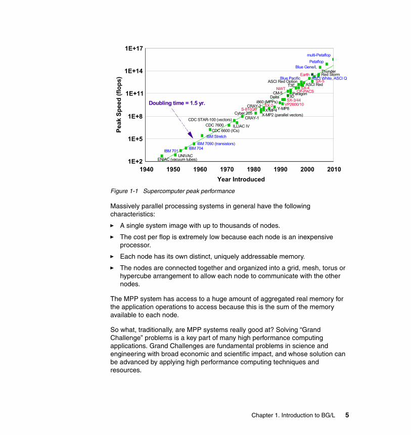
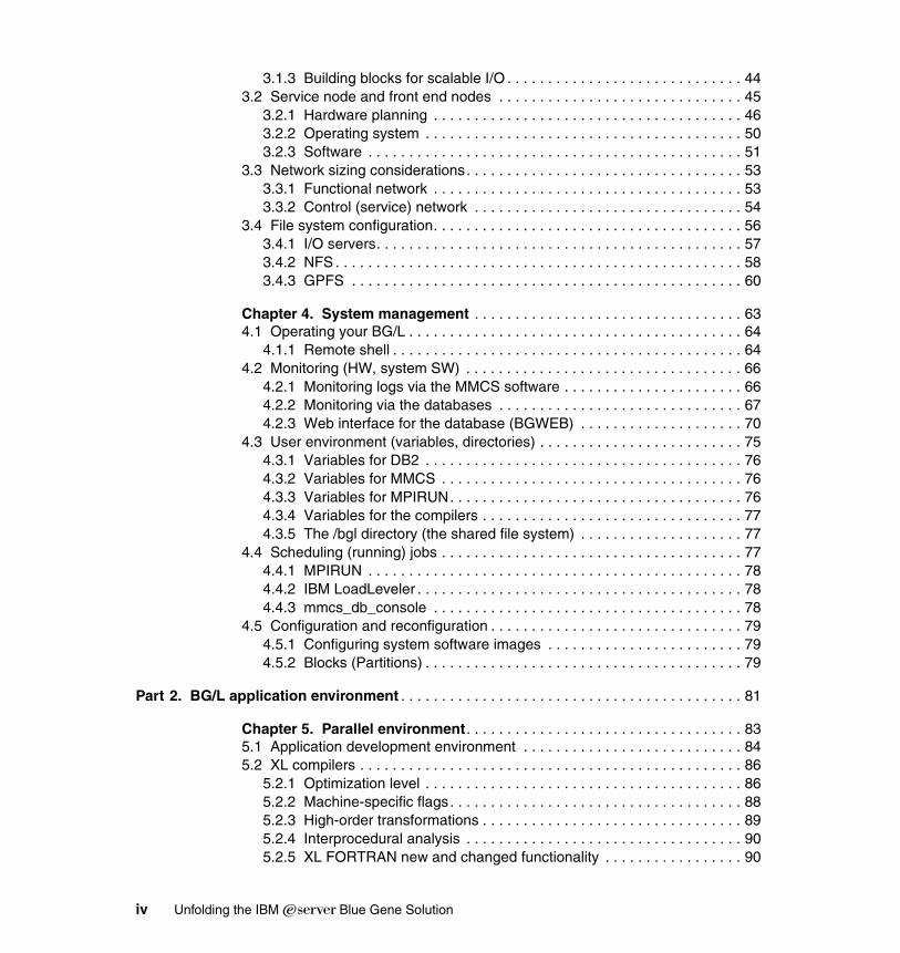
Figure 1-1 Supercomputer peak performance

Massively parallel processing systems in general have the following characteristics:

� A single system image with up to thousands of nodes.

� The cost per flop is extremely low because each node is an inexpensive processor.

� Each node has its own distinct, uniquely addressable memory.

� The nodes are connected together and organized into a grid, mesh, torus or hypercube arrangement to allow each node to communicate with the other nodes.

The MPP system has access to a huge amount of aggregated real memory for the application operations to access because this is the sum of the memory available to each node.

So what, traditionally, are MPP systems really good at? Solving “Grand Challenge” problems is a key part of many high performance computing applications. Grand Challenges are fundamental problems in science and engineering with broad economic and scientific impact, and whose solution can be advanced by applying high performance computing techniques and resources.

1940 1950 1960 1970 1980 1990 2000 2010Year Introduced

1E+2

1E+5

1E+8

1E+11

1E+14

1E+17

Peak

Spe

ed (f

lops

)

Doubling time = 1.5 yr.

ENIAC (vacuum tubes)UNIVAC

IBM 701 IBM 704IBM 7090 (transistors)

IBM StretchCDC 6600 (ICs)

CDC 7600CDC STAR-100 (vectors) CRAY-1

Cyber 205 X-MP2 (parallel vectors)

CRAY-2X-MP4Y-MP8

i860 (MPPs)

ASCI White, ASCI Q

PetaflopBlue Gene/L

Blue Pacific

DeltaCM-5 Paragon

NWT

ASCI Red OptionASCI Red

CP-PACS

Earth

VP2600/10SX-3/44

Red Storm

ILLIAC IV

SX-2

SX-4

SX-5

S-810/20

T3D

T3E

multi-Petaflop

Thunder

Chapter 1. Introduction to BG/L 5

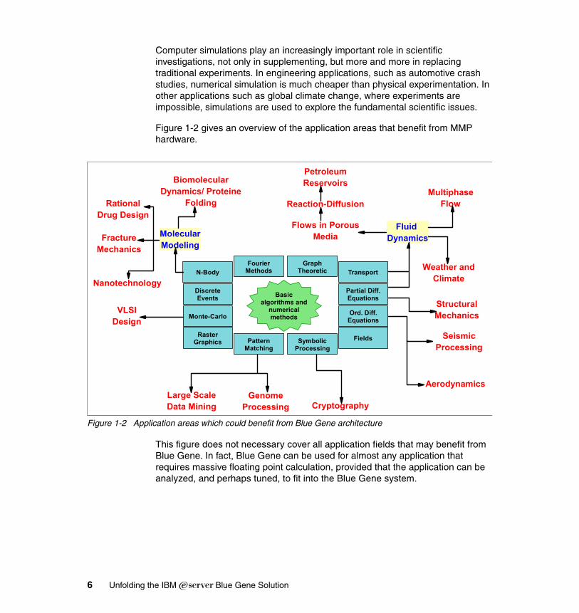
Computer simulations play an increasingly important role in scientific investigations, not only in supplementing, but more and more in replacing traditional experiments. In engineering applications, such as automotive crash studies, numerical simulation is much cheaper than physical experimentation. In other applications such as global climate change, where experiments are impossible, simulations are used to explore the fundamental scientific issues.

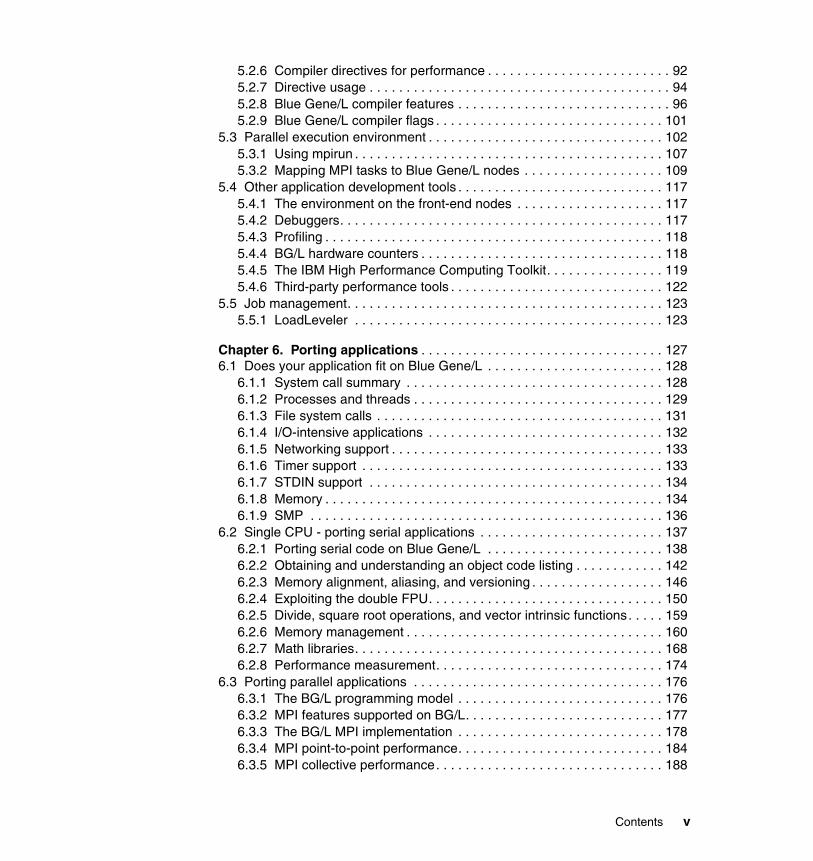
Figure 1-2 gives an overview of the application areas that benefit from MMP hardware.

Figure 1-2 Application areas which could benefit from Blue Gene architecture

This figure does not necessary cover all application fields that may benefit from Blue Gene. In fact, Blue Gene can be used for almost any application that requires massive floating point calculation, provided that the application can be analyzed, and perhaps tuned, to fit into the Blue Gene system.

Basic algorithms and

numerical methods

Fourier Methods

Graph Theoretic

Pattern Matching

Symbolic Processing

Transport

Partial Diff. Equations

Ord. Diff. Equations

Fields

N-Body

Discrete Events

Monte-Carlo

Raster Graphics

MolecularModeling

BiomolecularDynamics/ Proteine

FoldingRationalDrug Design

FractureMechanics

Nanotechnology

VLSIDesign

GenomeProcessing

Large ScaleData Mining Cryptography

SeismicProcessing

Aerodynamics

StructuralMechanics

Fluid Dynamics

MultiphaseFlow

Weather andClimate

Reaction-Diffusion

Flows in PorousMedia

PetroleumReservoirs


1.2 Overview of the IBM eServer Blue Gene SolutionDuring 4Q05, IBM announced the commercial availability of the IBM eServer Blue Gene Solution, a commercial version of the research project. This is a full rack system that can deliver (in the initial implementation) a peak performance of 5.7 Teraflops.

Multiple racks are designed to be linked together to function as a single computer yielding one third of a Petaflop. Based on IBM’s Power architecture, the IBM eServer Blue Gene Solution is optimized for bandwidth, scalability, and the ability to handle large amounts of data while consuming a fraction of the electric power and floor space required by today's fastest systems.

Blue Gene/L is IBM's first step in the journey to reach a 1 Petaflop computation target, and also is a new entrant into the already rich IBM Deep Computing portfolio.

Blue Gene/L is a newcomer to the ever-changing High Performance Computing landscape. It is only natural for everyone to take a critical look at the newcomer to determine what it is and what it is not, what it can and cannot do, and of course, how it measures up against the established players in this field. BlueGene/L is no exception.

Blue Gene/L already represents a phenomenal leap in the supercomputer race, with a peak performance of 70+ Teraflops for 16 linked Blue Gene/L racks (32 K processors), giving it the number one spot on the Top 500 Supercomputers list (http://www.top500.org/). We can expect Blue Gene/L to have a long-term presence on this landscape since the first fully populated system is expected to reach 64 racks (128k processors) with a peak rate over 360 Teraflops.

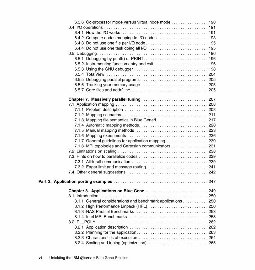
From a practical point of view, Blue Gene/L is built starting with dual CPU (processor) chips placed in pairs on a compute card together with 2 x 512MBytes of RAM (512MB for each dual core chip). The compute card is placed on a 16 card plane (node card) which is inserted into a dual-sided 16-slot midplane. Two such midplanes are hosted in a rack. These racks are then linked together. Figure 1-3 shows this build up.


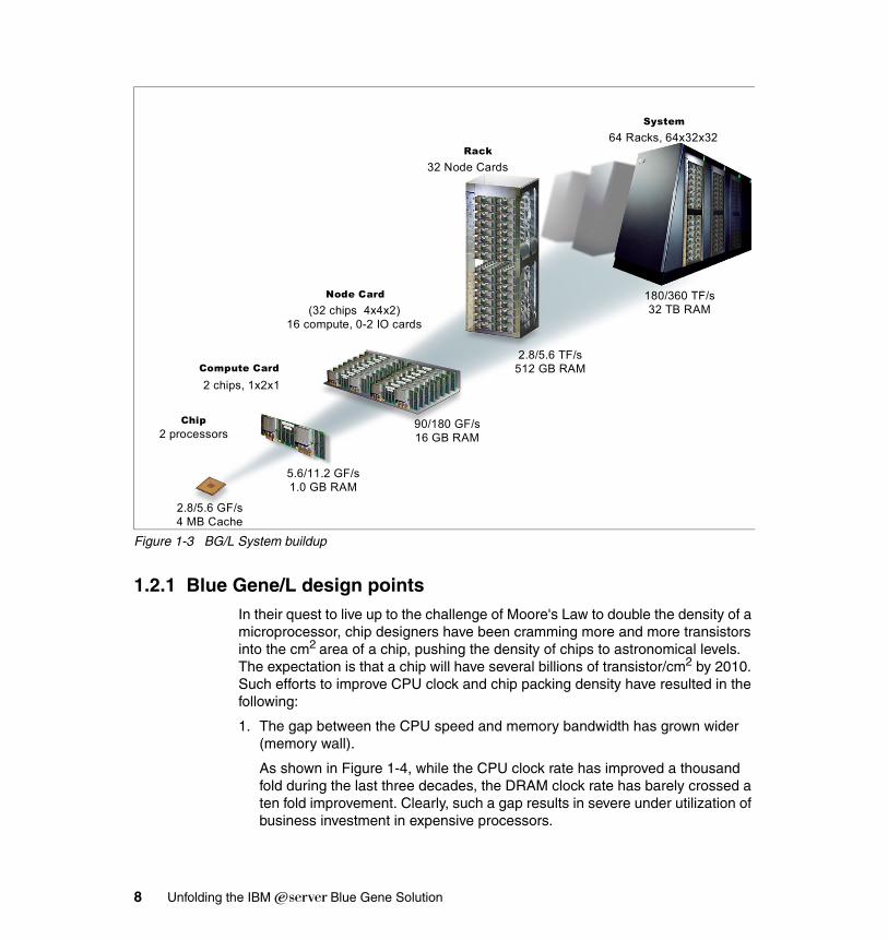
Figure 1-3 BG/L System buildup

1.2.1 Blue Gene/L design pointsIn their quest to live up to the challenge of Moore's Law to double the density of a microprocessor, chip designers have been cramming more and more transistors into the cm2 area of a chip, pushing the density of chips to astronomical levels. The expectation is that a chip will have several billions of transistor/cm2 by 2010. Such efforts to improve CPU clock and chip packing density have resulted in the following:

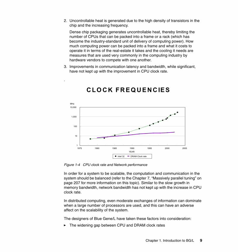
1. The gap between the CPU speed and memory bandwidth has grown wider (memory wall).

As shown in Figure 1-4, while the CPU clock rate has improved a thousand fold during the last three decades, the DRAM clock rate has barely crossed a ten fold improvement. Clearly, such a gap results in severe under utilization of business investment in expensive processors.

2.8/5.6 GF/s4 MB Cache

2 processors

2 chips, 1x2x1

5.6/11.2 GF/s1.0 GB RAM

(32 chips 4x4x2)16 compute, 0-2 IO cards

90/180 GF/s16 GB RAM

32 Node Cards

2.8/5.6 TF/s512 GB RAM

64 Racks, 64x32x32

180/360 TF/s32 TB RAM

Rack

System

Node Card

Compute Card

Chip


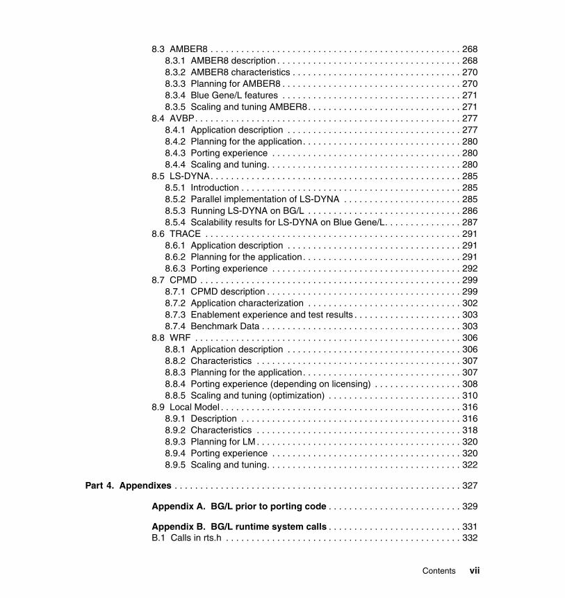
2. Uncontrollable heat is generated due to the high density of transistors in the chip and the increasing frequency.

Dense chip packaging generates uncontrollable heat, thereby limiting the number of CPUs that can be packed into a frame or a rack (which has become the industry-standard unit of delivery of computing power). How much computing power can be packed into a frame and what it costs to operate it in terms of the real-estate it takes and the cooling it needs are measures that are used very commonly in the computing industry by hardware vendors to compete with one another.

3. Improvements in communication latency and bandwidth, while significant, have not kept up with the improvement in CPU clock rate.

.

Figure 1-4 CPU clock rate and Network performance

In order for a system to be scalable, the computation and communication in the system should be balanced (refer to the Chapter 7, “Massively parallel tuning” on page 207 for more information on this topic). Similar to the slow growth in memory bandwidth, network bandwidth has not kept up with the increase in CPU clock rate.

In distributed computing, even moderate exchanges of information can dominate when a large number of processors are used, and this can have an adverse affect on the scalability of the system.

The designers of Blue Gene/L have taken these factors into consideration:

� The widening gap between CPU and DRAM clock rates

C LO C K FR E Q U E N C IE S

1975 1980 1985 1990 1995 2000 2005

YEAR

1

10

100

1,000

10,000

MHz

Intel 32 DRAM-Clock rate


� Excessive heat generated by dense packaging and high switching frequency

� The disparity between the CPU clock rate and the immediate vicinity peripheral devices (memory, I/O buses, and so forth)

� Network performance

The speed of the CPU is traded in favor of dense packaging and low power consumption per processor. The result is Blue Gene/L.

Each frame of Blue Gene/L consists of 1024 chips, where each chip has two modified PowerPC® 440s running at 700 MHz. These chips are connected by five networks, some of which offer latency as low as 4 microseconds and bandwidth of 350 Mb/sec. All this is packaged within a single rack with a power consumption of 28.14 kWh (per rack)!

The Blue Gene/L is designed to implement a parallel programming model based on Message Passing Interface.

Clearly, Blue Gene/L is not a the kind of “general purpose” supercomputer we are familiar with in the computing industry today. The CPU used here has a much lower clock frequency than other players in the field such as AMD Opteron, IBM POWER, and Intel Pentium® 4. Also, it has not been designed to run server OS’s like LINUX or AIX®. Thus, you should realize that the applications that can be run on this supercomputer are of a very specific scientific and technical nature.

On the other hand, recent research has shown that for most high performance computing applications, the current function and the associated overhead provided by operating systems such as AIX and LINUX is not needed. In other words, once a compute-intensive application is started it should not be interrupted by the operating system daemons. Such interruptions involve context switches, and context switches are expensive in CPU cycles.

This knowledge, coupled with the lack of need for most of the functions provided by a contemporary multi-tasking OS, has allowed the size of the kernel running on a Blue Gene/L processor to be reduced significantly. This results in an extremely low OS-related overhead, and the user program runs uninterrupted by the OS in a single tasking mode. Practically, the kernel which runs on a compute node is only capable of running a single task (process) at a moment in time.


1.2.2 Where does BlueGene/L fit into the pictureFor ease of discussion, we classify the applications that are considered for implementation on Blue Gene/L into the following categories:

Extremely suitableApplications in this class are highly “parallelizable” where the computer models are very large, with inter-process (task) communication requirements that scale so that the application can scale to several thousands of processors. The computational resource requirements for these applications are fixed throughout the duration of their execution. These applications typically have little or no interaction with the external environment other than occasional checkpointing of their state for processing continuation or restart.

Moderately suitableThis is the class of applications where the amount of effective parallelism is in the range of using 128 CPUs to 256 CPUs, with some limited interactions such as I/O or database. Although each job may not be using the complete Blue Gene/L network capabilities, having multiple jobs of this kind executing simultaneously on the system can be viewed as good utilization of Blue Gene/L. Some of these applications can migrate into being very good candidates for Blue Gene/L if the models used in these applications grow very large. Crash and Computational Fluid Dynamics (CFD) simulations are examples of this application set.

Not suitableSince the Blue Gene/L processor is significantly slower than its counterparts in today’s supercomputers, Blue Gene/L is not a suitable architecture to implement applications which are inherently serial or with very little parallelism. In addition, if it were even possible, running 2048 serial applications on 2048 Blue Gene/L processors packed into one frame would be an extreme case of under utilization of expensive investment tied up in the sophisticated communication network in Blue Gene/L.

Furthermore, when you run a serial application, you bar anyone from using any other processor of your partition. Currently, the smallest partition is 32 nodes, and some schedulers will not even consider partitions smaller than 512 nodes, so there is tremendous waste of processing potential.

Since the OS facilities (such as sockets and I/O to interface extensively with the external environment) are limited, applications that demand such interfaces may not be suitable for implementation on Blue Gene/L. Because Blue Gene/L is designed to run a tightly knit parallel application, there is no facility for the external environment to initiate interaction with the processes running inside Blue Gene/L(other than killing the entire job). All applications with such needs are not


suitable to run on Blue Gene/L. Examples of such applications are OLTP transactions initiated by an external system.

Applications that require dynamic allocation/reallocation of resources, such as CPUs or nodes, during the course of the computation are also not suitable for the current implementation of Blue Gene/L. Finally, applications that can’t tolerate failures are not suitable candidates for Blue Gene/L. This system aims for speed, not redundancy.


Chapter 2. Blue Gene/L architecture

In this chapter we describe the IBM Eserver Blue Gene Solution architecture. We begin with an overview of the machine, and then describe each piece of hardware. To end the chapter, the software layer is introduced to explain how it all works together.

This redbook gives a global view of the system. For in-depth knowledge of the hardware and software refer to:

� BlueGene/L: Hardware Installation and Serviceability, ZG24-5002

� Blue Gene/L: Software Installation, Configuration, and Administration, SG24-6744

2


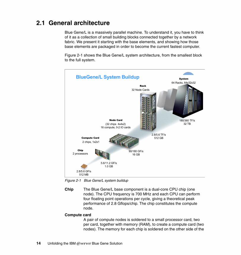
2.1 General architectureBlue Gene/L is a massively parallel machine. To understand it, you have to think of it as a collection of small building blocks connected together by a network fabric. We present it starting with the base elements, and showing how those base elements are packaged in order to become the current fastest computer.

Figure 2-1 shows the Blue Gene/L system architecture, from the smallest block to the full system.

Figure 2-1 Blue Gene/L system buildup

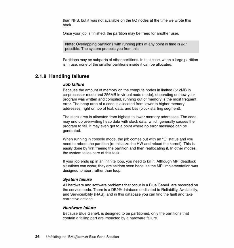
Chip The Blue Gene/L base component is a dual-core CPU chip (one node). The CPU frequency is 700 MHz and each CPU can perform four floating point operations per cycle, giving a theoretical peak performance of 2.8 Gflops/chip. The chip constitutes the compute node.

Compute card A pair of compute nodes is soldered to a small processor card, two per card, together with memory (RAM), to create a compute card (two nodes). The memory for each chip is soldered on the other side of the

2/17/2005 14

BlueGene/L System Buildup

2.8/5.6 GF/s512 MB

2 processors

2 chips, 1x2x1

5.6/11.2 GF/s1.0 GB

(32 chips 4x4x2)16 compute, 0-2 IO cards

90/180 GF/s16 GB

32 Node Cards

2.8/5.6 TF/s512 GB

64 Racks, 64x32x32

180/360 TF/s32 TB

Rack

System

Node Card

Compute Card

Chip


processor card; the amount of RAM per card is 1 GB (512 MB per compute node).

I/O card The I/O card is very similar to the compute card. A pair of compute nodes is soldered to a small processor card, two per card, together with memory (RAM), to create a compute card (two nodes). The memory for each chip can be soldered, in this case, on both sides of the card, for up to 2GB RAM per card (1GB per node). In addition, the I/O card has the integrated ethernet enabled (for communicating with the outside world).

Compute Node card The processor cards are plugged on a node card. There are two rows of eight compute cards on the node card (planar). You can also add two or four I/O nodes to a node card, but these are optional on each node card.

Midplane The processor cards, which bear 16 compute cards, are stacked in a midplane that sits in a rack.

Rack A rack holds two midplanes, for a total of 32 compute cards.

System You can connect up to 64 racks for your Blue Gene/L system.

System buildupThe number of processors in a machine is computed this way:

(number of racks) x (number of node cards per rack) x (number of compute cards per node card) x (number of processors per compute card)

That is:

(number of racks) x 32 x 16 x 4 = (number of racks) x 2048.

The actual largest configuration contains (64 x 2048) = 131072 processors.

This is a slightly simplified view of Blue Gene/L. In order for the system to be efficient, we need to connect the nodes to each other with a network. We describe this network further in 2.1.6, “Communications” on page 19.

You may have noticed that up to now we only mentioned CPU and memory. This is the core of the computing power, but for the entire system to work, we also need to be able to perform I/O operations. This is achieved through the I/O node that connect to the outside world through a gigabit ethernet network (also known as a functional network).

Note: We do not count the I/O processors because they do not contribute to the computation power (they do only I/O operations).

Chapter 2. Blue Gene/L architecture 15

Blue Gene/L is connected to the outside world via several components: one service node, one or more front-end nodes, and a global file system.

2.1.1 Nodes (Compute, I/O)As previously mentioned, nodes are made of one dual core chip soldered in pairs on a small card with 2 x 512 MB of memory.

The nodes do not have local persistent storage (file system), therefore, they must use outside storage for I/O operations. In order to reach the outside world, a compute node goes through an I/O node.

The hardware for both types of nodes is virtually identical, they only differ in the way they are used (there may be also extra RAM on the I/O nodes, and the physical connectors ar different). A compute node runs a light, UNIX-like proprietary kernel (compute node kernel - CNK); all system calls for I/O are shipped to one I/O node.

The I/O node is connected to the outside world through an ethernet port to the gigabit (functional) network and can perform file I/O operations.

We need a way to administer the machine, and a way for users to connect to it and submit jobs. We examine these topics in the following sections.

2.1.2 Blue Gene/L environmentFigure 2-2 presents an overview of the components of a IBM Eserver Blue Gene Solution environment.

Note: The only way to exchange data and to load programs into the Blue Gene/L system is through file I/O operations. There is no interactive I/O (keyboard, mouse) with the compute and I/O nodes.

Moreover, the compute nodes do not perform file I/O operations (they are not connected to the functional network).


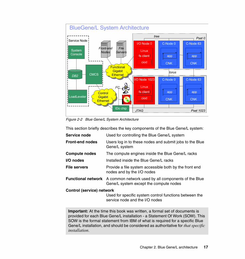
Figure 2-2 Blue Gene/L System Architecture

This section briefly describes the key components of the Blue Gene/L system:

Service node Used for controlling the Blue Gene/L system

Front-end nodes Users log in to these nodes and submit jobs to the Blue Gene/L system

Compute nodes The compute engines inside the Blue Gene/L racks

I/O nodes Installed inside the Blue Gene/L racks

File servers Provide a file system accessible both by the front end nodes and by the I/O nodes

Functional network A common network used by all components of the Blue Gene/L system except the compute nodes

Control (service) networkUsed for specific system control functions between the service node and the I/O nodes

Important: At the time this book was written, a formal set of documents is provided for each Blue Gene/L installation - a Statement Of Work (SOW). This SOW is the formal statement from IBM of what is required for a specific Blue Gene/L installation, and should be considered as authoritative for that specific installation.

BlueGene/L System Architecture

Functional Gigabit

Ethernet

Functional Gigabit

Ethernet

I/O Node 0

Linux

ciod

C-Node 0

CNK

I/O Node 1023

Linux

ciod

C-Node 0

CNK

C-Node 63

CNK

C-Node 63

CNK

Control Gigabit

Ethernet

Control Gigabit

Ethernet

IDo chip

LoadLeveler

SystemConsole

CMCS

JTAG

torus

tree

DB2

Front-endNodes

Pset 1023

Pset 0

I2C

FileServers

fs client

fs client

Service Node

app app

appapp


The following sections present general guidelines which should apply to all Blue Gene/L installations.

2.1.3 The service node (one per Blue Gene/L system)The service node is the manager of the Blue Gene/L solution. Beware, the term node may be misleading, since this is not one of the Blue Gene/L compute or I/O nodes, but a separate pSeries server (or an LPAR) running Linux.

The service node keeps track of the entire configuration and enables you to initiate any action on the Blue Gene/L system. This node allows you to manage Blue Gene/L, partition it, boot the nodes in any partition, and submit jobs to them.

2.1.4 One or more front-end nodesYou do not want to tie up Blue Gene/L resources for everyday interactive tasks. Since the only I/O possible is file I/O, there is no way to log on to Blue Gene/L. The users connect to front-end nodes to interact with the system. Here again, the term node may be misleading, because the front-end nodes are not part of the Blue Gene/L system, they are standalone pSeries Linux servers (or LPARs).

Since the nodes do not run a full-featured operating system, and there is no compiler on the nodes, jobs must be cross-compiled on the front-end nodes (or any other pSeries system running Linux or AIX) with a cross-compiler capable of generating code for the Blue Gene/L processor (a modified PPC440).

Jobs can only be submitted on the front-end nodes; the service node allocates the necessary resources on Blue Gene/L for them to run.

2.1.5 File systemSince all programs and data are prepared outside of the Blue Gene/L system, and there are no local disks inside the system, we need a global file system shared by the Blue Gene/L system (via I/O nodes), the service node, and the front-end nodes.

Currently, this global file system is mounted from an NFS server on the service node, on the front-end nodes, and on each I/O node of the Blue Gene/L system (every time a partition is booted).

Important: This is an important part of the machine and must not come as an afterthought. If you are architecting a solution, refer to Section 3.2, “Service node and front end nodes” on page 45.


An embedded GPFS (General Parallel File System - IBM’s high performance cluster file system) client for the I/O node is currently under development, this would eventually lift the limitations in the NFS model.

2.1.6 CommunicationsThis part is divided because the subject covers two completely different functionalities. There are two types of communications:

� High performance network for efficient parallel execution

� Connection to the outside world

High performance networkIn parallel computing there are two characteristics of the network that are of interest:

Bandwidth How many megabytes of data can one send from a node to another node in a second

Latency How long does it take for the first byte sent from one node to reach its target node

These two values characterize one link. On many high performance computing clusters today, the network fabric is assimilated to a switch. That is, we consider that all nodes are connected to all nodes and all links have the same speed. We view it as a full crossbar, but this is usually not true beyond 64 nodes or even on smaller configurations, although it is a good approximation. As the number of nodes grows, it is more and more complex to achieve the full structure, and less and less efficient.

Instead of implementing a single type of network capable of transporting all protocols needed in such an environment, the Blue Gene/L has implemented separate networks for different types of communications.

The torus networkOn Blue Gene/L we are not using a switch but a 3D torus. Unfortunately, a 3D torus cannot be drawn in a readable way. In order to understand what it is, let us first look at a 3D mesh.


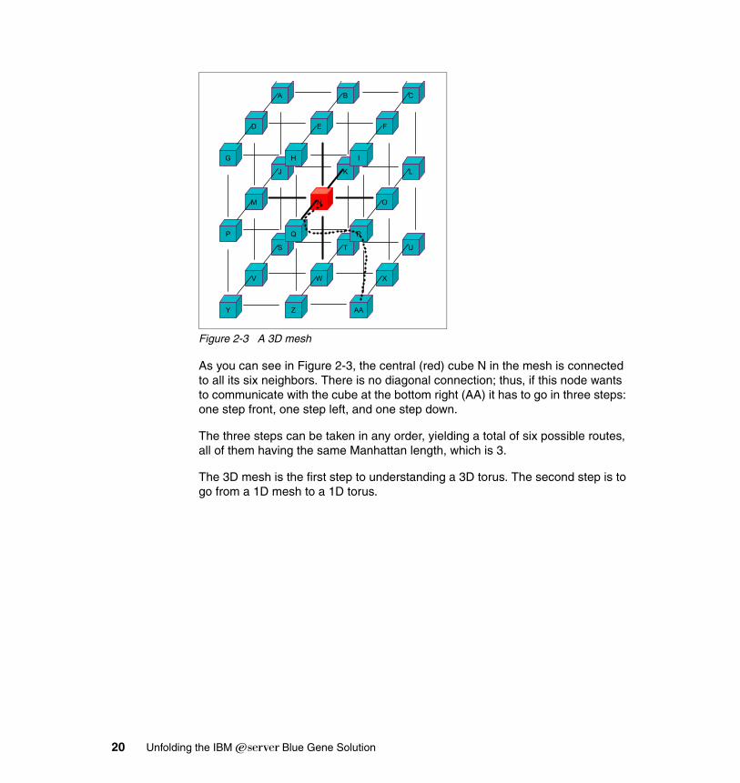
Figure 2-3 A 3D mesh

As you can see in Figure 2-3, the central (red) cube N in the mesh is connected to all its six neighbors. There is no diagonal connection; thus, if this node wants to communicate with the cube at the bottom right (AA) it has to go in three steps: one step front, one step left, and one step down.

The three steps can be taken in any order, yielding a total of six possible routes, all of them having the same Manhattan length, which is 3.

The 3D mesh is the first step to understanding a 3D torus. The second step is to go from a 1D mesh to a 1D torus.

A B C

J K L

S T U

D E F

M N O

V W X

G H I

P Q R

Y Z AA


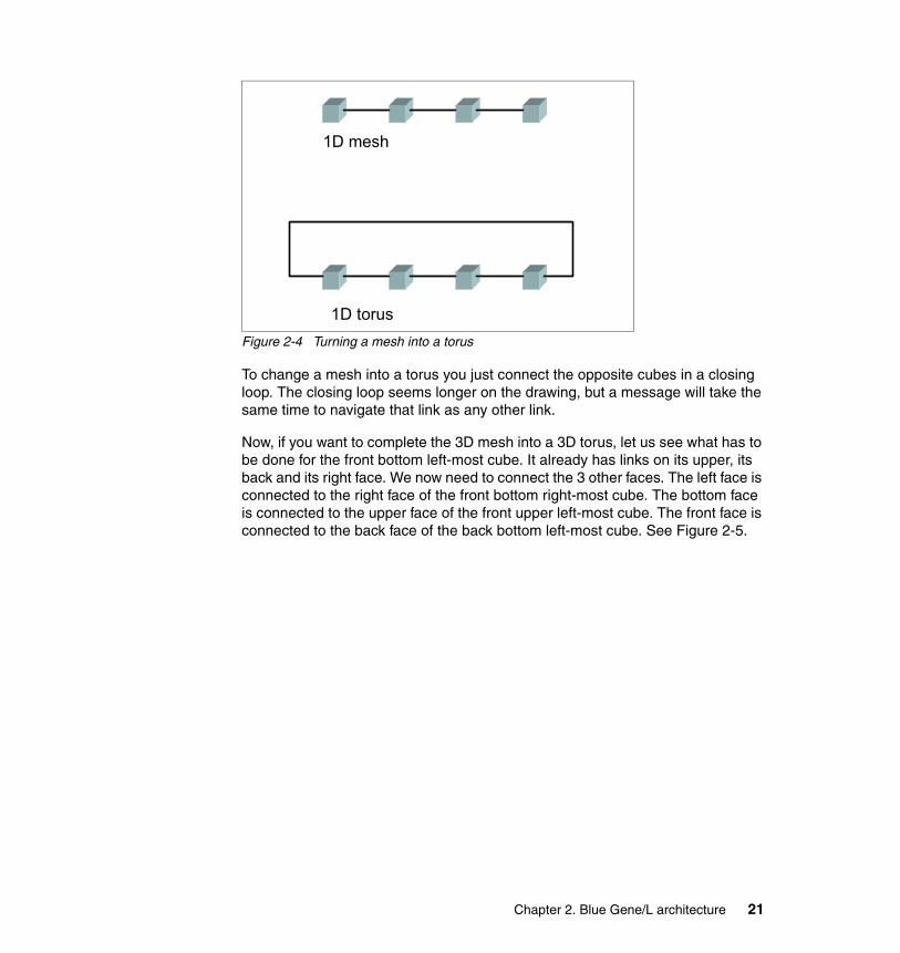
Figure 2-4 Turning a mesh into a torus

To change a mesh into a torus you just connect the opposite cubes in a closing loop. The closing loop seems longer on the drawing, but a message will take the same time to navigate that link as any other link.

Now, if you want to complete the 3D mesh into a 3D torus, let us see what has to be done for the front bottom left-most cube. It already has links on its upper, its back and its right face. We now need to connect the 3 other faces. The left face is connected to the right face of the front bottom right-most cube. The bottom face is connected to the upper face of the front upper left-most cube. The front face is connected to the back face of the back bottom left-most cube. See Figure 2-5.

1D mesh

1D torus


Figure 2-5 Building the 3D torus

Imagine the same pattern of connections was added to all cubes at the edges and the corners of the torus. All cubes are now connected to 6 neighbors. The cubes in the drawing represent compute nodes. In Figure 2-6 you can see a more elaborate torus comprised of 64 compute nodes (in this case cubes have been replaced with spheres).

A B C

J K L

S T U

D E F

M N O

V W X

G H I

P Q R

Y Z AA


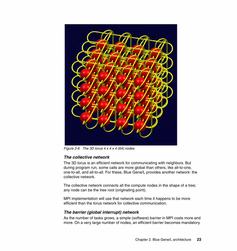
Figure 2-6 The 3D torus 4 x 4 x 4 (64) nodes

The collective networkThe 3D torus is an efficient network for communicating with neighbors. But during program run, some calls are more global than others, like all-to-one, one-to-all, and all-to-all. For these, Blue Gene/L provides another network: the collective network.

The collective network connects all the compute nodes in the shape of a tree; any node can be the tree root (originating point).

MPI implementation will use that network each time it happens to be more efficient than the torus network for collective communication.

The barrier (global interrupt) networkAs the number of tasks grows, a simple (software) barrier in MPI costs more and more. On a very large number of nodes, an efficient barrier becomes mandatory.


The barrier (global interrupt) network is the third dedicated hardware network Blue Gene/L provides for efficient MPI communication.

Connection to the outside worldAll interactions between the Blue Gene/L compute nodes and the outside world are carried through the I/O nodes under the control of the service node. There are two networks connecting the service node to the I/O nodes:

� A gigabit network (gigabit (functional) network)

� The service network (essentially another ethernet network, but converted to the internal jtag network via the service cards)

The gigabit network (gigabit (functional) network)This network is used to mount the global file system to allow Blue Gene/L access to file I/O. The I/O node further communicates to compute nodes through the collective network.

The service network (jtag network)The jtag network grants the service node direct access to the Blue Gene/L nodes. It is used to boot the nodes (initialize the hardware, load the kernel, and so forth). Each node card has a chip that converts the JTAG connections coming from both compute and I/O nodes into a 100Mbps ethernet network, which is further connected to the service node.

2.1.7 Execution environmentThe end-user environment is the front-end node, which is a pSeries server running Linux used for cross-compiling (to produce executable code for the compute nodes). Cross-compiling is not very different from compiling, it just uses different compiler options, and creates an executable that cannot run on the front-end node but runs on the Blue Gene/L compute nodes. You just need to use the proper FC or CC value in your makefile, and maybe some FFLAGS, CFLAGS, and LDFLAGS as well, to generate the executable you need for Blue

Important: If you are designing the architecture for a Blue Gene/L solution, do not forget that this implies the use of one or more ethernet switches that have to be properly sized. For more information refer to Section 3.3, “Network sizing considerations” on page 53.

Note: The global file system only has to be “global” to all the nodes in a partition, plus the service node and the front end node used to submit the job. You may have different file systems for different partitions (if needed).


Gene/L. Details about compiling a job are provided in Chapter 5, “Parallel environment” on page 83.

To run an application on Blue Gene/L, you need a mechanism to schedule the job. There are currently three ways to execute a program:

� LoadLeveler

� mpirun

� Directly submitting a job from the BG/L console (running on the service node)

In all cases, the executable is started on a set of Blue Gene/L processors. The sets are defined by the system administrator when Blue Gene/L is installed and configured. These sets are called partitions.

One partition is entirely dedicated to your job; it is even rebooted before your job is started. Boot time usually takes only a few seconds. No one else has access to your partition while your job is running. The communication networks inside a partition (torus, collective, global interrupt) are isolated from the rest of Blue Gene/L.

Since your job needs data (read and write), this has to reside on an NFS file system that is mounted on Blue Gene/L I/O nodes, and also mounted on the front-end node, so that you can prepare the files from your environment on the front-end node. The standard error and standard output (job results) are also created on the specified file system.

There are plans to use General Parallel File System (GPFS) on the I/O nodes, as client nodes to external GPFS servers. GPFS will provide better I/O performance

Attention: At the time this material was written, we were mostly using console mode to allocate partitions and submit jobs. In that mode it is possible to access partitions that are smaller than a midplane (512 nodes/1024 processors).

The smallest partition we could use was a node card (32 nodes/64 processors). When a partition is smaller than a midplane, the 3D torus cannot be created (some nodes in that partition do not have six neighbors); you only have a 3D mesh. When a partition is a single node card, the mesh is 2D. But, with such a small configuration, having to use a mesh instead of a torus does not generate much overhead.

Note: Allocating less than a midplane may not be supported in normal customer environments.


than NFS, but it was not available on the I/O nodes at the time we wrote this book.

Once your job is finished, the partition may be freed for another user.

Partitions may be subparts of other partitions. In that case, when a large partition is in use, none of the smaller partitions inside it can be allocated.

2.1.8 Handling failures

Job failureBecause the amount of memory on the compute nodes in limited (512MB in co-processor mode and 256MB in virtual node mode), depending on how your program was written and compiled, running out of memory is the most frequent error. The heap area of a code is allocated from lower to higher memory addresses, right on top of text, data, and bss (block starting segment).

The stack area is allocated from highest to lower memory addresses. The code may end up overwriting heap data with stack data, which generally causes the program to fail. It may even get to a point where no error message can be generated.

When running in console mode, the job comes out with an “E” status and you need to reboot the partition (re-initialize the HW and reload the kernel). This is easily done by first freeing the partition and then reallocating it. In other modes, the system takes care of this task.

If your job ends up in an infinite loop, you need to kill it. Although MPI deadlock situations can occur, they are seldom seen because the MPI implementation was designed to abort rather than loop.

System failureAll hardware and software problems that occur in a Blue Gene/L are recorded on the service node. There is a DB2® database dedicated to Reliability, Availability, and Serviceability (RAS), and in this database you can find the fault and take corrective actions.

Hardware failureBecause Blue Gene/L is designed to be partitioned, only the partitions that contain a failing part are impacted by a hardware failure.

Note: Overlapping partitions with running jobs at any point in time is not possible. The system protects you from this.


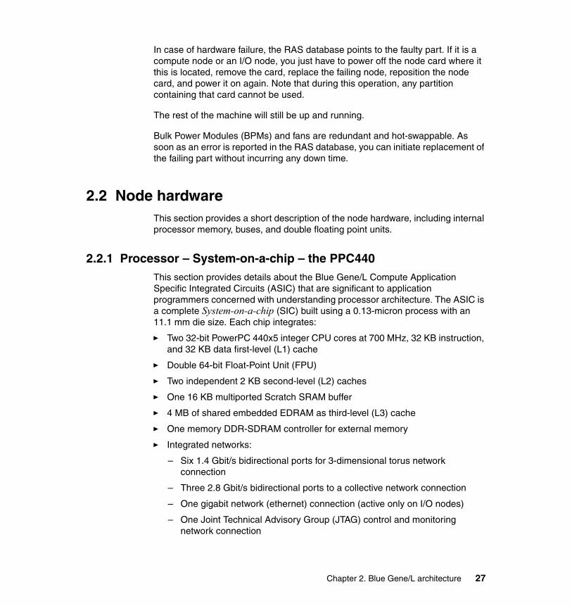
In case of hardware failure, the RAS database points to the faulty part. If it is a compute node or an I/O node, you just have to power off the node card where it this is located, remove the card, replace the failing node, reposition the node card, and power it on again. Note that during this operation, any partition containing that card cannot be used.

The rest of the machine will still be up and running.

Bulk Power Modules (BPMs) and fans are redundant and hot-swappable. As soon as an error is reported in the RAS database, you can initiate replacement of the failing part without incurring any down time.

2.2 Node hardware This section provides a short description of the node hardware, including internal processor memory, buses, and double floating point units.

2.2.1 Processor – System-on-a-chip – the PPC440This section provides details about the Blue Gene/L Compute Application Specific Integrated Circuits (ASIC) that are significant to application programmers concerned with understanding processor architecture. The ASIC is a complete System-on-a-chip (SIC) built using a 0.13-micron process with an 11.1 mm die size. Each chip integrates:

� Two 32-bit PowerPC 440x5 integer CPU cores at 700 MHz, 32 KB instruction, and 32 KB data first-level (L1) cache

� Double 64-bit Float-Point Unit (FPU)

� Two independent 2 KB second-level (L2) caches

� One 16 KB multiported Scratch SRAM buffer

� 4 MB of shared embedded EDRAM as third-level (L3) cache

� One memory DDR-SDRAM controller for external memory

� Integrated networks:

– Six 1.4 Gbit/s bidirectional ports for 3-dimensional torus network connection

– Three 2.8 Gbit/s bidirectional ports to a collective network connection

– One gigabit network (ethernet) connection (active only on I/O nodes)

– One Joint Technical Advisory Group (JTAG) control and monitoring network connection


– One barrier (global interrupt) network connection

The Blue Gene/L compute ASIC chip includes two non cache-coherent microprocessors, each containing one single load/store unit, one single 32-bit integer unit and one double Single-Instruction-Multiple-Data (SIMD) 64-bit FPU. Each FPU can execute up to two multiply-adds per cycle, meaning that the peak performance is eight 64-bit floating-point operations per cycle, resulting in 2.8 Gflops/s per core and 5.6 Flops/s per chip.

Figure 2-7 shows the different components of the Blue Gene/L Compute ASIC.

Note: The memory system is coherent (shared) only beyond the L1 caches. The first-level (L1) cache is inside the PowerPC 440 embedded microprocessor core. The PowerPC 440 microprocessor does not offer shared memory support capability (it is not a true SMP implementation). The L2 cache has a snoop coherency mechanism and the L3 cache is shared between the two processors, and is therefore coherent.


Figure 2-7 Blue Gene/L Compute ASIC

2.2.2 Blue Gene/L PowerPC 440 core overviewThe PowerPC440 (PPC440) core is a flexible and powerful implementation of the full 32-bit BOOK-E Enhanced PowerPC Architecture. The original design of the PPC440 does not contain a floating point unit. Interfaces for custom co-processors and floating point function are provided, along with separate 32KB/32KB instruction and data cache array interfaces. Figure 2-8 shows the components of the PPC440 core. The relevant features of the core include:

� High-performance, dual-issue, superscalar 32-bit RISC CPU

� Seven stage, highly pipelined micro-architecture

� Dual instruction fetch per cycle, decode, and out-of-order issue

PLB (4:1)

“Double FPU”

Ethernet Gbit

JTAGAccess

144 bit wide DDR256/512MB

JTAG

Gbit Ethernet

440 CPU

440 CPUI/O proc

L2

L2

MultiportedSharedSRAM Buffer

Torus

DDR Control with ECC

SharedL3 directoryfor EDRAM

Includes ECC

4MB EDRAM

L3 CacheorMemory

6 out and6 in, each at 1.4 Gbit/s link

256

256

1024+144 ECC256

128

128

32k/32k L1

32k/32k L1

“Double FPU”

256

snoop

Collective


GlobalInterrupt

4 global barriers orinterrupts

128

5.5GB/s

2.7GB/s

11GB/s

22GB/s

PLB (4:1)

“Double FPU”

Ethernet Gbit

JTAGAccess

144 bit wide DDR256/512MB

JTAG

Gbit Ethernet

440 CPU

440 CPUI/O proc

L2

L2

MultiportedSharedSRAM Buffer

Torus

DDR Control with ECC

SharedL3 directoryfor EDRAM

Includes ECC

4MB EDRAM

L3 CacheorMemory


256

256

1024+144 ECC256

128

128

32k/32k L1

32k/32k L1

“Double FPU”

256

snoop

Collective


GlobalInterrupt

4 global barriers orinterrupts

128

5.5GB/s

2.7GB/s

11GB/s

22GB/s


� Three independent execution pipelines:

– Combined complex integer, system, and branch pipeline

– Simple integer pipeline

– Load/store pipeline

� Dynamic branch prediction

� Single cycle multiply and multiple-accumulate

� Two replicated 6 port 32x32-bit General Purpose Register (GPR) files

� 32 KB instruction and 32KB data L1 caches

� 64-entry, fully associative unified translation look-aside buffer (TLB)

� Three independent 128-bit Processor Local Buses (PLBs) for instruction reads, data reads, and data writes, running at half the processor speed

� 128-bit Auxiliary Processor Unit (APU), running at the processor speed

� 128-bit load/store interface supporting APU execution of floating point instructions (direct access between APU and L1 data cache)

APU load and store instructions directly access the L1 cache, with operands of up to one quadword (16 bytes) in length.

The instruction cache controller can make 32-byte line read requests through the PLB instruction read interface, and can also present quadword burst read requests for up to three lines (six quadwords), as part of its speculative line fill mechanism. The 128-bit read and write PLB interface can make requests for 32-byte lines, as well as for 1-15 bytes within a 16-byte (quadword) aligned region.


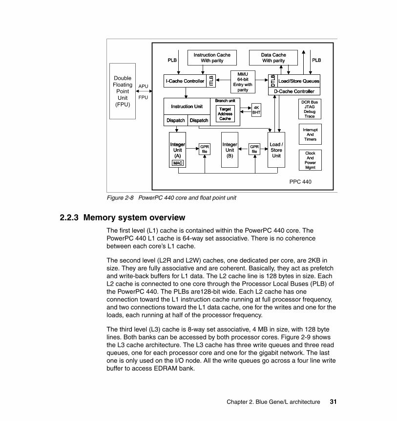
Figure 2-8 PowerPC 440 core and float point unit

2.2.3 Memory system overviewThe first level (L1) cache is contained within the PowerPC 440 core. The PowerPC 440 L1 cache is 64-way set associative. There is no coherence between each core’s L1 cache.

The second level (L2R and L2W) caches, one dedicated per core, are 2KB in size. They are fully associative and are coherent. Basically, they act as prefetch and write-back buffers for L1 data. The L2 cache line is 128 bytes in size. Each L2 cache is connected to one core through the Processor Local Buses (PLB) of the PowerPC 440. The PLBs are128-bit wide. Each L2 cache has one connection toward the L1 instruction cache running at full processor frequency, and two connections toward the L1 data cache, one for the writes and one for the loads, each running at half of the processor frequency.

The third level (L3) cache is 8-way set associative, 4 MB in size, with 128 byte lines. Both banks can be accessed by both processor cores. Figure 2-9 shows the L3 cache architecture. The L3 cache has three write queues and three read queues, one for each processor core and one for the gigabit network. The last one is only used on the I/O node. All the write queues go across a four line write buffer to access EDRAM bank.

Instruction CacheWith parity

Data CacheWith parity

I-Cache Controller

ITLB Load/Store Queues

DTL

B

D-Cache Controller

MMU64-bit

Entry withparity

4KBHT

TargetAddressCache

Branch unitInstruction Unit

Dispatch Dispatch

DCR BusJTAGDebugTrace

ClockAnd

PowerMgmt

InterruptAnd

Timers

GPRfile

IntegerUnit(B)

Load /StoreUnit

IntegerUnit(A)MAC

GPRfile

PLBPLBInstruction Cache

With parityData CacheWith parity

I-Cache Controller

ITLBI-Cache Controller

ITLB Load/Store Queues

DTL

B

D-Cache Controller

Load/Store Queues

DTL

B

D-Cache Controller

MMU64-bit

Entry withparity

4KBHT

TargetAddressCache


Dispatch Dispatch

TargetAddressCache

Branch unit

TargetAddressCache


Dispatch Dispatch

DCR BusJTAGDebugTrace

ClockAnd

PowerMgmt

InterruptAnd

Timers

GPRfile

IntegerUnit(B)

Load /StoreUnit

IntegerUnit(A)MAC

IntegerUnit(A)MAC

GPRfile

PLBPLB

PPC 440

DoubleFloating

PointUnit

(FPU)

APU

FPU


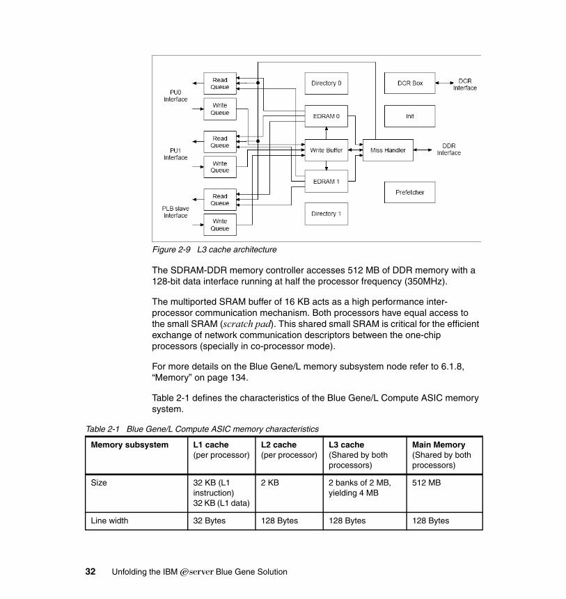
Figure 2-9 L3 cache architecture

The SDRAM-DDR memory controller accesses 512 MB of DDR memory with a 128-bit data interface running at half the processor frequency (350MHz).

The multiported SRAM buffer of 16 KB acts as a high performance inter- processor communication mechanism. Both processors have equal access to the small SRAM (scratch pad). This shared small SRAM is critical for the efficient exchange of network communication descriptors between the one-chip processors (specially in co-processor mode).

For more details on the Blue Gene/L memory subsystem node refer to 6.1.8, “Memory” on page 134.

Table 2-1 defines the characteristics of the Blue Gene/L Compute ASIC memory system.

Table 2-1 Blue Gene/L Compute ASIC memory characteristics

Memory subsystem L1 cache(per processor)

L2 cache(per processor)

L3 cache(Shared by both processors)

Main Memory(Shared by both processors)

Size 32 KB (L1 instruction)32 KB (L1 data)

2 KB 2 banks of 2 MB, yielding 4 MB

512 MB

Line width 32 Bytes 128 Bytes 128 Bytes 128 Bytes


2.2.4 Double floating point unit overviewTh design of this unit is also known as Oedipus architecture.

Unlike POWER4™ or POWER5™ chips, the Blue Gene/L processor chip does not provide two independent FPUs; instead, it provides a double SIMD FPU, including parallel primary and secondary arithmetic pipes with its own 32 x 64-bit floating point register (FPR) file.

The primary pipe executes the standard instructions and the SIMD instructions while the second pipe only executes the SIMD instructions. The double FPU implemented on Blue Gene/L chip offers more capabilities than a pure SIMD unit. Some instructions cause two different operations to be performed in the two pipes.

For example, the instructions allow efficient support for complex cross products. Other instructions cause a single operation to occur on a single set of data. The instruction set is given in Appendix C, “Floating point instruction set” on page 341.

The results from the pipes are only written to the corresponding FPRs: primary FPRs for the primary pipe, and secondary FPRs for the secondary pipe. However, the cross micro architecture of FPU, illustrated in Figure 2-10, allows

Number of lines 1024 16 32768

Coherent No yes (weakly) yes yes

Associativity 64 way fully 8 way/bank2 banks

NA

Latency (in cycles)

3 11 28/36/40(hit/miss precharged/miss busy)

86 (L3 cache enabled)

Sustained bandwidth,random quadLoadaccess (Bytes/cycle)

NA NA 1.28/1.2(hit/miss)

0.8/0.5(single/dual processor)

Sustained bandwidth,sequential quadLoadaccess (Bytes/cycle)

16 5.3 5.3/5.3(hit/mis)

5.1/3.4(single/dual processor)

Memory subsystem L1 cache(per processor)

L2 cache(per processor)

L3 cache(Shared by both processors)

Main Memory(Shared by both processors)


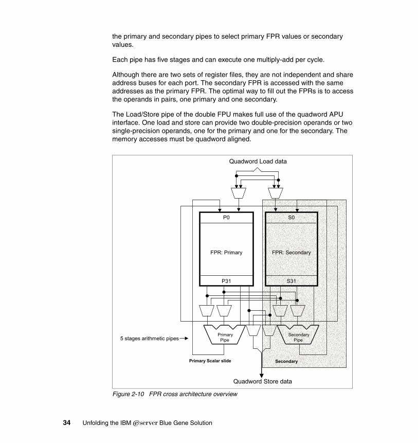
the primary and secondary pipes to select primary FPR values or secondary values.

Each pipe has five stages and can execute one multiply-add per cycle.

Although there are two sets of register files, they are not independent and share address buses for each port. The secondary FPR is accessed with the same addresses as the primary FPR. The optimal way to fill out the FPRs is to access the operands in pairs, one primary and one secondary.

The Load/Store pipe of the double FPU makes full use of the quadword APU interface. One load and store can provide two double-precision operands or two single-precision operands, one for the primary and one for the secondary. The memory accesses must be quadword aligned.

Figure 2-10 FPR cross architecture overview

PrimaryPipe

P0

FPR: Primary

P31

SecondaryPipe

S0

FPR: Secondary

S31

Primary Scalar slide Secondary

Quadword Store data

Quadword Load data

5 stages arithmetic pipes


2.3 Blue Gene/L SoftwareThis section describes the software stack (unique to BG/L) that runs on the compute and I/O nodes, and also provides a short introduction to the Midplane Management Control System (MMCS).

2.3.1 System softwareThe system software consists of the following two kernels:

� Compute node kernel - CNK (also known as the Blue Gene Runtime System or BLRTS)

� I/O node kernel

Compute node kernel The kernel that runs on the compute node is called the compute node kernel (CNK). This is a small, simple kernel that provides a Linux-like run-time environment, but it is IBM proprietary. It has a subset of the Linux system calls. Most of those system calls are related to I/O, so you can open and close, read and write, create directories and symbolic links, and so forth. For details see Chapter 6, “Porting applications” on page 127.

The CNK has about 30 to 40 percent of the Linux system calls (for details, refer to Chapter 2, “System calls supported by Compute Node Kernel” in the redbook Blue Gene/L: Application Development, SG24-6745). This kernel is a single user, single process run time and has no paging mechanism. The compute node communicates to the outside world through the I/O node, so the executable program is loaded from the I/O node through the collective network.

I/O node kernelThe kernel of the I/O node is also called the Mini-Control Program (MCP). It is a port of the Linux Kernel, which means it is GPL/LGPL licensed. It has specific patches for the Blue Gene Architecture, such as:

� Patches for Blue Gene/L� New interrupt controller (BIC)� Save-and-restore for dual FPU registers on context switch� New memory layout� New set of Device Control Registers (DCRs)� Driver for new Ethernet macro (EMAC4 based on EMAC3)

The I/O service is provided to the compute nodes from the compute node I/O daemon (CIOD), which is started by the initialization script during the boot procedure of the MCP. CIOD is a user-level process that controls and services


applications in the compute node and interacts with the Midplane Management and Control System(MMCS).

2.3.2 Management softwareThe Blue Gene/L management software is based on a a set of databases running on the service node (database software is DB2).

Midplane Management Control System (MMCS)Both Blue Gene/L hardware and software are controlled and managed by the Midplane Management Control System (MMCS). The service node, front-end nodes, and the file servers are not under the control of MMCS. MMCS currently consists of several daemons which interact with a DB2 database running on the service node.

DaemonsThe three main daemons are idoproxydb, mmcs_db_server and ciodb. These programs run on the service node and have the following functions:

� idoproxydb: Handles the communication to the cluster hardware

� mmcs_db_server: Manages the blocks (also known as partitions), handles the requests from mmcs_db clients (mmcs_db_console, mmcs_db command scripts or a job scheduler)

� ciodb: Detects the block when it is initialized and manages the job submission request

For more details about the MMCS software refer to Chapter 11, “Midplane Management Control System (MMCS)” in the redbook Blue Gene/L: Software Installation, Configuration, and Administration, SG24-6744.

DB2 databasesThere are four DB2 databases that interact with the MMCS on the service node.

� Configuration database: Records Blue Gene/L component location and connectivity. Most items in this database relate to specific physical pieces of hardware.

� Operational database: Records partitions, job status, and events related to ongoing Blue Gene/L system activity. Although called one of the four databases, the operational database is actually part of the configuration database.

� Environmental database: Records periodic readings of voltage levels, switch settings, and sensors.


� Reliability, Availability, Serviceability (RAS) database: Records both software- and hardware-related errors. It is the RAS database that is most closely watched by system administrators keeping an eye on the overall system health.



Chapter 3. Planning and sizing guidelines

This chapter provides general guidelines for designing the environment around an IBM Eserver Blue Gene Solution, such as:

� Service node and front-end nodes

� Sizing – network considerations

� File system configuration

3


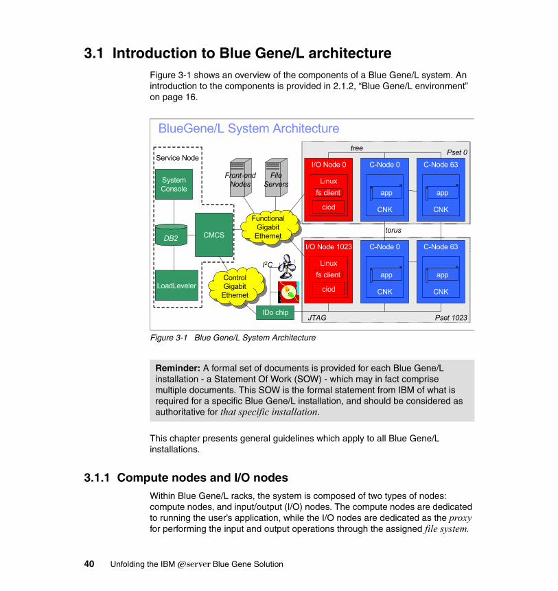
3.1 Introduction to Blue Gene/L architectureFigure 3-1 shows an overview of the components of a Blue Gene/L system. An introduction to the components is provided in 2.1.2, “Blue Gene/L environment” on page 16.

Figure 3-1 Blue Gene/L System Architecture

This chapter presents general guidelines which apply to all Blue Gene/L installations.

3.1.1 Compute nodes and I/O nodesWithin Blue Gene/L racks, the system is composed of two types of nodes: compute nodes, and input/output (I/O) nodes. The compute nodes are dedicated to running the user’s application, while the I/O nodes are dedicated as the proxy for performing the input and output operations through the assigned file system.

Reminder: A formal set of documents is provided for each Blue Gene/L installation - a Statement Of Work (SOW) - which may in fact comprise multiple documents. This SOW is the formal statement from IBM of what is required for a specific Blue Gene/L installation, and should be considered as authoritative for that specific installation.

BlueGene/L System Architecture

Functional Gigabit

Ethernet

Functional Gigabit

Ethernet

I/O Node 0

Linux

ciod

C-Node 0

CNK

I/O Node 1023

Linux

ciod

C-Node 0

CNK

C-Node 63

CNK

C-Node 63

CNK

Control Gigabit

Ethernet

Control Gigabit

Ethernet

IDo chip

LoadLeveler

SystemConsole

CMCS

JTAG

torus

tree

DB2

Front-endNodes

Pset 1023

Pset 0

I2C

FileServers

fs client

fs client

Service Node

app app

appapp


The compute node kernel contains stubs of I/O calls, and these stubs forward the I/O calls from the compute node stub to the I/O node assigned to that compute node. This allows for offloading some of the work for the compute nodes, frees up more memory for use by the user application in the compute nodes, and reduces the memory requirement of the compute node kernel itself.

Compute node modesThe compute nodes are, in fact, implemented as a pair of CPUs on a single chip, with 512 MB of dedicated RAM in which the user’s application runs. The compute nodes may be configured at boot time in one of following ways:

� Virtual node mode (VN)

This configuration uses both CPUs separately, running a different process of the user’s application on each processor. In this mode, the 512 MB memory is split between the two processors, giving each processor effectively 256 MB of memory for the compute node kernel and user application. Each processor also handles its own I/O interactions for messages and the file system I/O stubs.

� Co-processor node mode (CO)

This configuration uses the secondary CPU as an offload coprocessor for processing the I/O of the main CPU. This reduces the burden on the main CPU, and frees up additional memory for the user application since the 512 MB of memory does not need to be divided as in virtual node mode. In co-processor node mode, the second CPU will not handle any file-based I/O, only application messaging, after the primary CPU starts.

� Hybrid node mode

This is a (non-default) configuration created by the programmer. It is also sometimes referred to as Communication Coprocessor Mode with Computation Offload (CO), and in this mode, the secondary processor functions as both an I/O coprocessor and a user application processor. This mode is of use for those programmers who don’t mind coding the application to work with both processors on the chip, and the details that go with performing such a task (details like catering to the lack of L1 cache coherence between the two processors in order to wring out the last 2 to 4 percent of speed possible in the Blue Gene/L system). Benefits here will be code-dependent in addition developer-dependent.

Chapter 3. Planning and sizing guidelines 41

Choosing one of the three configuration modes can affect the I/O of the partition, depending on the application, and certainly affects the messaging capability.

I/O nodesThe input/output (I/O) nodes are very similar to the compute nodes. They also consist of a pair of CPUs, additional chips, memory, and gigabit Ethernet connections. In fact, the CPUs on the I/O node are the same as the ones used in the compute nodes. The I/O node runs a different kernel than the compute nodes, one that allows for file I/O (with a remote file system). The I/O node is the file system proxy for the compute nodes, the place where all the file system interaction is forwarded to and from the compute nodes.

3.1.2 Compute node to I/O node ratioSince the I/O nodes are the only method Blue Gene/L partitions can use to communicate with the outside world, the ratio of I/O nodes to compute nodes should be considered in the context of the user applications I/O and the overall configuration of a Blue Gene/L system. Each node card can have up to two I/O nodes, but you do not need to use all these nodes for performing I/O operations. This means that you can use one I/O cards per eight compute nodes (8-to-1 ratio), or you can use a reduced number of I/O nodes for a larger number of compute nodes, up to a ratio of 64-to-1.

The currently allowable ratios are: 8-to-1, 16-to-1, 32-to-1, and 64-to-1.

Note: Hybrid node mode was used in the configuration for the Linpack run that scored 70.72 Tflop/s to bring Blue Gene/L to the top of the “Top 500 Super Computer List” in November, 2004.

This mode was used because a performance improvement of 2 to 4 percent over virtual node mode was observed, and a 4 percent performance improvement equates to approximately the total performance of the 66th system on that list (roughly 3 Tflops).

Although 4 percent may seem like a small number (because of the enormous capability of Blue Gene/L), the actual coding effort could be justified since the same absolute performance increase obtainable by adding additional hardware is much more expensive, and increases complexity and power consumption.

Restriction: The following information shows a 128-to-1 configuration ratio as well. Although technically possible, this may not be supported by IBM, and has only been used in internal test environments.


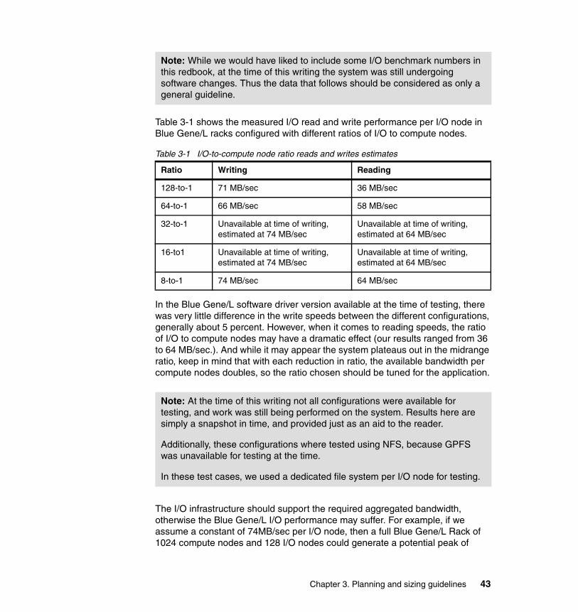
Table 3-1 shows the measured I/O read and write performance per I/O node in Blue Gene/L racks configured with different ratios of I/O to compute nodes.

Table 3-1 I/O-to-compute node ratio reads and writes estimates

In the Blue Gene/L software driver version available at the time of testing, there was very little difference in the write speeds between the different configurations, generally about 5 percent. However, when it comes to reading speeds, the ratio of I/O to compute nodes may have a dramatic effect (our results ranged from 36 to 64 MB/sec.). And while it may appear the system plateaus out in the midrange ratio, keep in mind that with each reduction in ratio, the available bandwidth per compute nodes doubles, so the ratio chosen should be tuned for the application.

The I/O infrastructure should support the required aggregated bandwidth, otherwise the Blue Gene/L I/O performance may suffer. For example, if we assume a constant of 74MB/sec per I/O node, then a full Blue Gene/L Rack of 1024 compute nodes and 128 I/O nodes could generate a potential peak of

Note: While we would have liked to include some I/O benchmark numbers in this redbook, at the time of this writing the system was still undergoing software changes. Thus the data that follows should be considered as only a general guideline.

Ratio Writing Reading

128-to-1 71 MB/sec 36 MB/sec


32-to-1 Unavailable at time of writing, estimated at 74 MB/sec

Unavailable at time of writing, estimated at 64 MB/sec

16-to1 Unavailable at time of writing, estimated at 74 MB/sec

Unavailable at time of writing, estimated at 64 MB/sec


Note: At the time of this writing not all configurations were available for testing, and work was still being performed on the system. Results here are simply a snapshot in time, and provided just as an aid to the reader.

Additionally, these configurations where tested using NFS, because GPFS was unavailable for testing at the time.

In these test cases, we used a dedicated file system per I/O node for testing.


9472MB/sec bandwidth (128 I/O nodes * 74MB/sec.). The good news here is that each I/O node has it own Ethernet cable, simplifying network load distribution.

3.1.3 Building blocks for scalable I/OBlue Gene/L can potentially demand large amounts of both peak and sustained I/O per rack, depending on the application, and this should be planned for. The planning should include not only the type of file system used, but also network switches and file servers, as well as any load external to Blue Gene/L that will be placed on the same I/O system. The recommended file system for Blue Gene/L is the GPFS file system, and the recommendations here use that assumption.

File server operating systemThe file system needs to have a number of file servers, and if these servers are used for implementing a GPFS file system, the operating systems must be either AIX or Linux. Even though the GPFS implementation we used for testing was a very basic one, it is important to have scalable performance, high reliability, and multi-NFS-export capabilities.

File system server hardwareThe system hardware requirement will vary depending on your bandwidth (you need enough CPU to drive the network and the storage traffic) and reliability requirements. One rule of thumb for sizing the amount of CPU needed for driving the bandwidth is about 1GHz per 100MB per second throughput (this is a very rough estimate, and your actual performance may vary significantly). Two solid systems we recommend as NFS (or NSD in the case of GPFS) servers are the IBM eServer pSeries 550 or OpenPOWER 720. Ideally, these should be paired for redundancy.

StorageFor the storage system, you need to size both the capacity (amount of storage needed) and the sustained aggregated throughput for the targeted applications. The system should include redundancy to help protect against hardware and environment outages. Choices for storage subsystems include the IBM DS4500 and DS4000 storage servers. For example, if you need 1200 MB/sec GPFS storage throughput, you need to use at least four DS4500 subsystems (each can sustain 300MB/second GPFS bandwidth).

NetworkIn addition to the storage requirements, matching network bandwidth is required to sustain the I/O for the Blue Gene/L system. Thus you may consider multiple gigabit Ethernet links for each file system server; otherwise, the bottleneck will


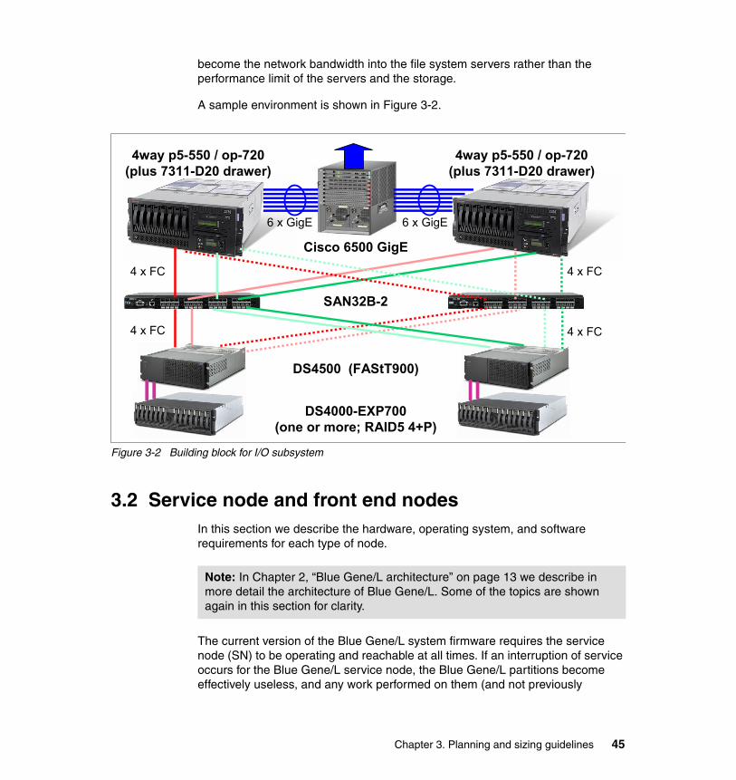
become the network bandwidth into the file system servers rather than the performance limit of the servers and the storage.

A sample environment is shown in Figure 3-2.

Figure 3-2 Building block for I/O subsystem

3.2 Service node and front end nodesIn this section we describe the hardware, operating system, and software requirements for each type of node.

The current version of the Blue Gene/L system firmware requires the service node (SN) to be operating and reachable at all times. If an interruption of service occurs for the Blue Gene/L service node, the Blue Gene/L partitions become effectively useless, and any work performed on them (and not previously

DS4000-EXP700(one or more; RAID5 4+P)

DS4500 (FAStT900)

SAN32B-2

Cisco 6500 GigE

4way p5-550 / op-720(plus 7311-D20 drawer)

4 x FC

4 x FC 4 x FC

4 x FC

6 x GigE

4way p5-550 / op-720(plus 7311-D20 drawer)

6 x GigE

Note: In Chapter 2, “Blue Gene/L architecture” on page 13 we describe in more detail the architecture of Blue Gene/L. Some of the topics are shown again in this section for clarity.


checkpointed) is lost. This version of Blue Gene/L system depends on the reliability of the service node.

The current version of the Blue Gene/L system firmware does not allow the use of more than one service node in a single Blue Gene/L system. This means the service node is effectively a single point of failure.

The front end nodes (FEN) are the point of entry for end users to the Blue Gene/L system. Users log on to a front end node, and compile programs and submit jobs from this node. The operation of the Blue Gene/L system does not depend on the front end nodes, but the performance and availability of the front end nodes will be directly visible to the system’s users.

The service node and front end nodes all run a Linux operating system on 64-bit PowerPC hardware (the current implementation is on SUSE Linux Enterprise Server 9).

3.2.1 Hardware planningThis section describes the hardware requirements for the service and front end nodes.

Service nodeThe service node currently runs on either POWER4 or POWER5 hardware.

For a Blue Gene/L system comprising between one and four racks, the guidelines for the service node are that it include at least:

� Two processors or more; a uniprocessor system is not recommended

� For a given pSeries model, the fastest processor speed available

� 32 GB of memory

� 146 GB of available disk storage in addition to the disks used for storing and booting the operating system

� Two 10/100 Ethernet adapters

� Two 10/100/1000 Ethernet adapters

The service node can run in a logical partition of a POWER4 pSeries server or can run in full SMP mode. LPAR mode allows the server hardware to be shared

Note: Refer to the formal “Statement Of Work Schedule A - Hardware Deliverables” for precise specifications of the hardware requirements for a specific installation.


between multiple operating system images, and one possibility would be to run the service node and the front end nodes in two LPARs on a single server such as a p650, p670 or p690.

Other considerations for the service node� If the hardware is dedicated to the service node, the service node can run in

full SMP mode (not in LPAR mode), and depending on the server hardware chosen, a Hardware Management Console may not be needed.

� If no HMC is provided, some kind of terminal and keyboard will probably be required to install the Linux operating system. Once the operating system is installed, the service node can be accessed and controlled via a network connection.

� If you are going to use LPAR, then we strongly recommend a rack-mounted HMC. This HMC is only one 19” EIA unit in size and can be installed in the same rack as the service node (depending on the pSeries model). There is also a rack-mounted keyboard/display kit available for the HMC which can be used as a single rack keyboard/display for the pSeries servers mounted in the rack as well (using a keyboard video mouse or KVM switch).

POWER5There are two basic POWER5 systems which can be considered:

� For a small Blue Gene/L system comprising a single rack, the OpenPower720 system with four processors is a good solution.

� For larger Blue Gene/L systems, the p5-570 provides an expandable platform (up to 16-way, but starting off as a 4-way system).

Front end nodes

Like the service node, the front end nodes run Linux on pSeries hardware; in this implementation they run SUSE Linux Enterprise Server 9 (SLES 9).

Multiple front end nodes can be installed. The front end nodes are used directly by users of the Blue Gene/L system. More than one front end node can be provided if a single front end node is not powerful enough to support the anticipated user load. There is no automatic load balancing or failover capability provided with multiple front end nodes, although an external network load balancer could be used to spread user load across multiple front end nodes.

Note: The plural “nodes” is used here because one front end node can be attached to a Blue Gene/L system, but using a single front end node is perfectly acceptable and may prove to be a better choice.


There is a much lower minimum capability requirement for a front end node compared to the requirement for the service node. A Blue Gene/L system can have a single front end node with sufficient capacity for all the users at the same time, or multiple front end nodes with the user load shared across the front end nodes in some way.

Many of the early Blue Gene/L systems have used IBM eServer BladeCenter® JS20 systems as front end nodes. These systems are dual CPU PPC970 processor blades that are housed in 7-U rack enclosures.

This configuration choice should not be taken as prescriptive. Having more than one front end node is only required if a single node is not capable of handling the expected user load by itself, and having more than one front end node increases the work of the systems administrator.

The front end nodes need network connectivity to a shared file system, which will also be used by the Blue Gene/L system.

Figure 3-1 on page 40 shows a logical picture of the components of a Blue Gene/L system. It would be perfectly possible for the separate external components—service node, front end nodes, and file server nodes—to have a physical implementation in a single server. With this in mind, the hardware for the front end nodes can be selected in two different ways: using the same hardware as the service node, and using separate hardware from the service node. These choices are described in the following sections.

Same hardware as the service nodeThe simplest configuration is to use a single server for both the service node and the front end node and use logical partitioning to construct two separate server instances running on a single server.

Size the server as the sum of the requirements of the service node and front end node.

For a combined front end node and service node a single unit (p650, p570, and so forth) or server with a split SCSI backplane and external HMC could be used: this system has 7 available PCI-X adapter slots and each partition can be configured with a 4-port 10/100 Ethernet adapter and a 2-port 10/100/1000 adapter to satisfy the network connectivity requirements of the server. Using the split SCSI backplane allows two separate logical partitions to boot from different internal disks.

Once the service node is supported on the SLES 9 platform, as well as the front end nodes, the choice of hardware for a common single server platform increases. A single p5-570 system will be a good single platform because it is


capable of expansion if the user load grows, or a p5-550 system may be a more economical choice.

Separate hardware from the service nodeThis configuration option increases the work of the systems administrator but allows alternative hardware platforms to be used for the front end nodes.

In addition to the hardware platforms already identified for the service node, the front end nodes can run on any other system which supports the ppc64 SUSE Linux Enterprise Server 9 (SLES 9) operating platform, and this means additionally:

� POWER5-based pSeries servers including both Open Power™ and p5 systems. The OpenPower 720 system with two processors would be a good starting point, and can be configured with four processors if user growth is anticipated.

� JS-20 BladeCenter systems, which are based on the POWERPC970 processor.

One initial installation based on JS20 blade systems has been configured with 4GB memory per node, so if the approach of using separate hardware from the service node for front end nodes is chosen, then each front end node should have this amount of memory at minimum.

It is obviously possible to implement a number of front end nodes in a BladeCenter rack of JS-20 blade servers, and many Blue Gene/L installations have chosen to do this. It is worth noting that this implementation decision is not mandatory, and the other options discussed in this chapter may prove more suitable to a specific Blue Gene/L system installation.

Don’t forget the rackThe service node and front end nodes will probably be rack-mounted models and therefore a rack needs to be provided for them.

Note: The front end nodes cannot run all platforms which are supported by SLES 9, they must run on POWER4, POWER5, or POWERPC970 processors.

Note: Although JS20 blades can be used as front end nodes, the limited I/O capabilities they provide require special attention during installation and configuration; thus, we recommend that you chose these systems only as an alternate solution.


If multiple systems are provided, can they be installed in the same rack? It might sound obvious, but even if the systems have the same 19” form factor, are there sufficient power distribution units (PDUs) of the correct type available in the rack? The IBM BladeCenter uses a different rack type and model, with different PDUs, from the pSeries rack. If you plan on using different server types, it may be necessary to plan for additional PDUs or alternative power cables if you want to fit all the servers in a single rack. If you don’t consider this aspect you run the risk of turning up at a customer site on the day of installation and discovering that it is not possible to install and power all the components necessary for the system.

FirmwareBe sure to check the required firmware level for each service node server and each front end node server to ensure that it matches the minimum necessary level of firmware for Blue Gene/L systems.

Early experience with Blue Gene/L systems using JS20 blade servers as front end nodes required a firmware update for supporting the Linux (SLES 9) to be installed.

3.2.2 Operating systemIf either the service node or the front end nodes are to be implemented on a POWER4 p655 platform, special attention needs to be given to the method of installing the operating system for the first time because there is no internal CD-ROM drive on the p655. An external network install server will need to be provided in this case, specifically AIX NIM or SUSE Yast installation server. Once the operating system has been installed it will be possible to configure addresses on the network adapters and further work can proceed in the same way as for any other type of server, except that of course there is still no CD-ROM drive and the install media will still have to be accessed across the network in some way.

Specific considerations apply to the service node and to the front end nodes, as explained in the following sections.

Note: Check the SOW documentation provided for your system and also any other specific operating systems and hardware requirements at the time of installation. Refer to:

http://www-1.ibm.com/servers/eserver/support/pseries/index.htmlhttp://www-1.ibm.com/servers/eserver/support/openpower/index.html


Service nodeCurrent implementation (at the time of writing this redbook) supports SUSE Linux Enterprise Server 9 (SLES 9), Service Pack 1 or later.

This software and its associated support contract need to be obtained separately; neither is included as part of the Blue Gene/L product shipped by IBM.

IBM provides the operating system kernels for the Blue Gene/L nodes as part of the BlueGene/L driver, and this software is installed on the service node because this code is downloaded into the Blue Gene/L nodes when the partition they are members of is started.

Front end nodesSUSE Linux Enterprise Server 9 (SLES 9) Service Pack 1or later.

As for the Service Node, this software and an associated support contract need to be obtained prior to implementation.

SLES 9 will run on POWER4, POWER5, and POWERPC970 (OpenPOWER) hardware.

3.2.3 SoftwareAdditional software needs to be obtained separately for both the service node and for the front end nodes, and in many cases this means purchasing licensed software and software maintenance agreements. The reason for stressing this point is, again, that the IBM installation team will expect this software to be available at installation time.

The service node needs different software to be installed on it than the front end nodes. The levels of code specified in this section are current as of 06/30/2005, but the “Statement of Work” documentation associated with a specific Blue Gene/L implementation should be treated as authoritative on the code levels required for that particular installation.

The front end nodes are used to compile code for Blue Gene/L. This requires all the compilers plus libraries applicable to Blue Gene/L to be available on the front end nodes.

Service nodeSoftware which needs a formal license agreement� DB2 UDB Enterprise Server V8.1 with Fixpack 7 or DB2 Enterprise Server

V8.2


� IBM Loadleveler (optional)

Software which does not need a formal license agreement� Java™ Runtime JRE 1.4.1 (This is actually bundled with SLES 9, so it does

not need to be obtained separately; just make sure the correct version is installed.)

� Python V2.3 or later

Front end nodesSoftware which needs a formal license agreement� IBM compilers: XL Fortran and XL C/C++ for Linux

Blue Gene/L versions of the libraries will be supplied and installed separately.

� IBM DB2 UDB Enterprise Server client: Delivered as part of the DB2 UDB Server product required for the service node.

� IBM Engineering and Scientific Subroutine Libraries (ESSL): Currently under development, so no formal product such as “ESSL for Blue Gene/L” exists today, but once it is formally released as a product it will need to be purchased separately.

� IBM LoadLeveler (optional).

� Etnus TotalView debugger (optional).

� UPC/CEPBA Paraver visualization tool (optional).

Software which does not need a formal license agreement� MPI library (MPICH2) V0.971

� Java Runtime JRE 1.4.1 (Optional on front end nodes, this is actually bundled with SLES 9 so it does not need to be obtained separately; just make sure the correct version is installed.)

� GNU Toolchain (glibc, gcc, binutils, gdb)

� Mathematical Acceleration Subsystem (MASS) libraries

IBM Eserver Blue Gene Solution softwareSoftware which needs some kind of formal license agreement� IBM General Parallel File System (GPFS) (This is optional, and not currently

supported.) GPFS client code will run on the I/O nodes.

Software which does not need a formal license agreement� The Compute Node Kernel (CNK) for the Blue Gene/L compute nodes and

Linux Kernel for the Blue Gene/L I/O nodes, which will be installed across the network from the Service Node when a Blue Gene/L partition is booted.


3.3 Network sizing considerationsBlue Gene/L requires two Ethernet networks, both of which are shown in Figure 3-1 on page 40. A single network switch could be used to provide the hardware for both networks, with a simple logical isolation approach such as port-based Virtual LANs (VLANs) being used to separate the two networks inside the single switch.

3.3.1 Functional networkWhen a user job is running on a Blue Gene/L partition, the only communication path to anything outside the Blue Gene/L rack uses the functional network.

In particular, this network is used for all file system I/O because there are no disks installed inside the Blue Gene/L rack.

All connections to the functional network are gigabit Ethernet connections using copper cables: 1000Base-T using Cat.6 cabling.

The functional network needs to provide connections for the following equipment:

� One connection for each I/O node in the Blue Gene/L rack; the default configuration is for 128 I/O nodes to be installed in every rack.

� One connection for each front end node.

� One connection for the service node.

� One or more connections to each file server. Figure 3-2 on page 45 shows a possible configuration in which six parallel gigabit Ethernet links are provided to each file server, configured as a logical single link using an aggregation technique (EtherChannel, or some kind of link aggregation).

� One or more external network connections, for which it may also be appropriate to provide a dedicated network firewall.

Network switch performanceThere are two basic types of Gigabit Ethernet switches available today: blocking and non-blocking switches.

Blocking switches are cheaper than non-blocking switches because they are designed to be able to handle an average network load spread across multiple ports.

Non-blocking switches are more expensive because they are designed to be able to handle the maximum network load on every port simultaneously.

This difference also applies to line cards installed in a switch chassis.


Blocking switches are suitable for collections of workstations that typically generate I/O requests at different times. This characteristic does not apply to Blue Gene/L, which will typically generate multiple simultaneous I/O requests from all its I/O nodes. The configuration of a network switch for the functional network needs to take this into account.

For example, Cisco provides a 48-port 10/100/1000BASE-T line card (WS-X4448-GB-RJ45), which can connect to 48 Blue Gene/L I/O nodes simultaneously. It needs to be understood that this particular card provides total networking capacity of 12GBps, or 6GBps full-duplex capacity. If all I/O nodes were working at full capacity they would require a total of 48GBps full-duplex capacity, in other words 8 times the capability of the line card.

Equally, in a modular switch such as the Cisco 4000/4500 series, the total capacity of the switch may be less than the total number of ports might imply: a single switch can support up to 240 ports of 10/100/1000BASE-T, but the total capacity of the switch is 64 Gbps.

This means it may be necessary to use more switches, or change to more expensive non-blocking switches, to cater for the peak bandwidth required between the Blue Gene/L I/O nodes and the file system infrastructure. Port density alone may not be the only criterion here: a single switch with provision for 240 ports may provide the necessary connectivity for the Blue Gene/L I/O nodes, but may act as a bottleneck to effective performance.

Jumbo framesIf possible, jumbo frames should be used across the functional network. This allows the Maximum Transmission Unit (MTU) for Ethernet frames to be increased from the default value of 1500 bytes to 9000 bytes. There are implementation considerations here, since not all Gigabit Ethernet network interface cards support this extension to the standard, hence the caveat if possible.

3.3.2 Control (service) networkThe control network is used for the service node to communicate with the service components of each Blue Gene/L rack.

The current implementation of the Service Node requires only 10/100 Ethernet ports, and needs connections to be made in two different ways:

1. To the first node only in a row of nodes, to the iDo network

2. To every separate midplane in the row of code


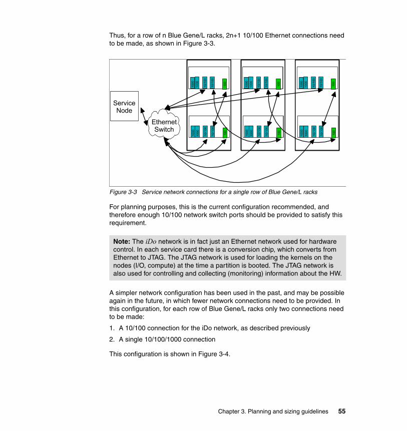
Thus, for a row of n Blue Gene/L racks, 2n+1 10/100 Ethernet connections need to be made, as shown in Figure 3-3.

Figure 3-3 Service network connections for a single row of Blue Gene/L racks

For planning purposes, this is the current configuration recommended, and therefore enough 10/100 network switch ports should be provided to satisfy this requirement.

A simpler network configuration has been used in the past, and may be possible again in the future, in which fewer network connections need to be provided. In this configuration, for each row of Blue Gene/L racks only two connections need to be made:

1. A 10/100 connection for the iDo network, as described previously

2. A single 10/100/1000 connection

This configuration is shown in Figure 3-4.

Note: The iDo network is in fact just an Ethernet network used for hardware control. In each service card there is a conversion chip, which converts from Ethernet to JTAG. The JTAG network is used for loading the kernels on the nodes (I/O, compute) at the time a partition is booted. The JTAG network is also used for controlling and collecting (monitoring) information about the HW.

Service Node

100

10/1

00

10/1

00

1000

1000

100

10/1

00

10/1

00

1000

1000

Ethernet Switch

100

10/1

00

10/1

00

1000

1000

100

10/1

00

10/1

00

1000

1000

100

10/1

00

10/1

00

1000

1000

100

10/1

00

10/1

00

1000

1000

100

10/1

00

10/1

00

1000

1000

100

10/1

00

10/1

00

1000

1000


Figure 3-4 Simpler Control Network configuration for a row of Blue Gene/L racks

The bandwidth requirements for the service network are not great, and relatively simple networking equipment can be used for the purpose. However, it is likely that for many configurations, using the same physical hardware as the network switch provided for the functional network will make sense.

3.4 File system configurationThe Blue Gene/L hardware has no disk subsystem of its own, and has been designed as a stateless system so that the nodes in a partition are fully operational once they have booted. All information about the state of the Blue Gene/L system is stored in the service node.

To make Blue Gene/L an operational system, some kind of common file system needs to be provided. This file system is accessed from the front end nodes and is used for storage of source code and for saving the executable files that result from the compilation process that takes place on the front end nodes.

When jobs run on Blue Gene/L, the I/O nodes have access to the same common file system and load the executable files across the Functional Network into the compute nodes. The file system is then used for writing results of the computation that takes place on the Blue Gene/L system.

Service Node

100

10/1

00

10/1

00

1000

1000

100

10/1

00

10/1

00

1000

1000

Ethernet Switch

100

10/1

00

10/1

00

1000

1000

100

10/1

00

10/1

00

1000

1000

100

10/1

00

10/1

00

1000

1000

100

10/1

00

10/1

00

1000

1000

100

10/1

00

10/1

00

1000

1000

100

10/1

00

10/1

00

1000

1000

Note: By convention, this common file system is mounted as /bgl on the front end nodes and on the Blue Gene/L nodes.


For the current implementation, the I/O node operating system only supports NFS client access to the common file system, thus the file servers should provide an NFS export of a local or a GPFS file system. Future releases will include in the I/O node embedded Linux a GPFS client. We will describe some of the possible approaches, starting with the simplest approach.

3.4.1 I/O serversA single Blue Gene/L rack contains up to 128 I/O nodes, each of which has a gigabit Ethernet connection into the functional network. Whether all of these I/O nodes are used depends on the code running on the Blue Gene/L compute nodes, but this means that there is the theoretical possibility of a single Blue Gene/L rack generating I/O requests of between 1GBps and 10GBps (and that’s gigabytes per second, not gigabits per second).

To reach the theoretical limit requires code that performs intensive I/O operations in a manner that spreads the I/O workload across all available I/O nodes, and this is by no means simple. Later in this book we discuss strategies for increasing I/O throughput, but the code modification necessary may not be accomplished quickly or easily.

It is vital to provide I/O servers that attach to the Blue Gene/L functional network so that their capability matches the requirements of the code running on the Blue Gene/L system.

For some codes, a single NFS server may be sufficient, and will certainly meet the functional requirement of the Blue Gene/L system.

However, a single NFS server using a single gigabit Ethernet connection will be limited to I/O performance of 60MBps at maximum, and this sort of figure has been measured in performance tests.

Since the theoretical limit of aggregate I/O capability by a single Blue Gene/L rack exceeds this single NFS server capability by many orders of magnitude, a single NFS server could represent a significant bottleneck to overall Blue Gene/L system performance.

The solution to this bottleneck is to provide more than one I/O server.


3.4.2 NFSThe only method of implementing a shared parallel file system today on Blue Gene/L is by providing an NFS server attached to the functional network. The Blue Gene/L I/O nodes are booted with a Linux kernel that includes an NFS client capability, and the I/O nodes issue an NFS mount command when they start up to attach to the shared file system.

By convention, the shared file system is mounted on the Blue Gene/L nodes and front end nodes at the /bgl mount point. Adhering to this convention makes it easier to understand someone else’s Blue Gene/L system, but it is not mandatory.

It may be a requirement of a particular Blue Gene/L implementation that the front end nodes and I/O nodes connect to an existing NFS shared file system. This is certainly possible.

Alternatively, it may be necessary to provide a new NFS server as part of a new Blue Gene/L system implementation.

The simplest approach would be to provide a single NFS server, and to implement this server on the service node if possible. There’s nothing to prevent an Intel-based Linux server with IDE disks being used for this purpose either, since the functional requirement is satisfied, but this sort of approach may be unwise in the long term because such servers may not be reliable enough and may not perform well enough as usage of the Blue Gene/L system increases.

Over time, however, a single NFS server may be an unacceptable bottleneck to system performance. With this approach, all the I/O nodes in the Blue Gene/L system will access the same server, and quite possibly at the same time. Codes

Important: It’s important when discussing I/O performance and capability to differentiate between the Blue Gene/L rack and the Blue Gene/L system as a whole. A single Blue Gene/L rack is capable of very high levels of I/O performance, but if the Blue Gene/L rack is not matched with an equally high performance I/O subsystem then the total system’s I/O performance may not be good and may not meet expectations.

So, saying that Blue Gene/L is not suited to applications which need high levels of I/O performance is incorrect, but one particular instance of a Blue Gene/L system implementation may not be suitable for applications which need high levels of I/O performance if the system as a whole is not configured for these levels of performance.


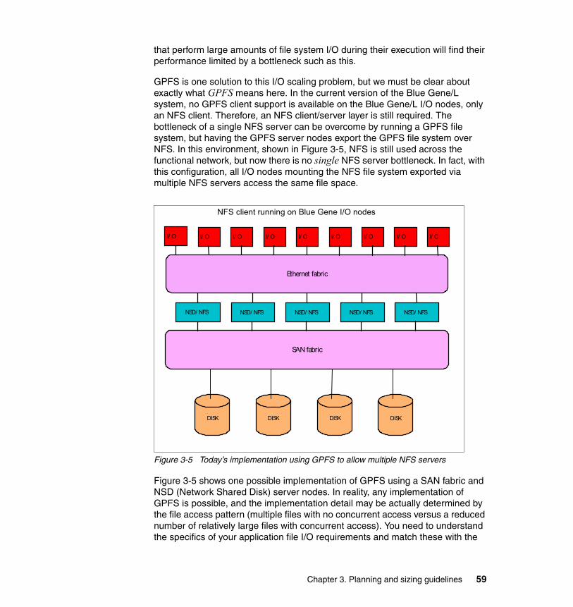
that perform large amounts of file system I/O during their execution will find their performance limited by a bottleneck such as this.

GPFS is one solution to this I/O scaling problem, but we must be clear about exactly what GPFS means here. In the current version of the Blue Gene/L system, no GPFS client support is available on the Blue Gene/L I/O nodes, only an NFS client. Therefore, an NFS client/server layer is still required. The bottleneck of a single NFS server can be overcome by running a GPFS file system, but having the GPFS server nodes export the GPFS file system over NFS. In this environment, shown in Figure 3-5, NFS is still used across the functional network, but now there is no single NFS server bottleneck. In fact, with this configuration, all I/O nodes mounting the NFS file system exported via multiple NFS servers access the same file space.

Figure 3-5 Today’s implementation using GPFS to allow multiple NFS servers

Figure 3-5 shows one possible implementation of GPFS using a SAN fabric and NSD (Network Shared Disk) server nodes. In reality, any implementation of GPFS is possible, and the implementation detail may be actually determined by the file access pattern (multiple files with no concurrent access versus a reduced number of relatively large files with concurrent access). You need to understand the specifics of your application file I/O requirements and match these with the

2

IBM Research

Blue Gene/L © 2004 IBM Corpo

DISK DISKDISK DISK

I/ O I/ O I/ O I/ O I/ O I/ O I/ O I/ O I/ O

Ethernet fabric

NSD/ NFS NSD/ NFS NSD/ NFS NSD/ NFS NSD/ NFS

SAN fabric

NFS client running on Blue Gene I/O nodes


proper GPFS configuration, because NFS is not able to provide any locking between NFS instances running on different nodes.

3.4.3 GPFSIBM is currently developing a GPFS client implementation for the Blue Gene/L I/O nodes. When available, this will allow NFS to be eliminated from the Blue Gene/L environment if desired, although it may be reasonable to continue to use NFS for the connections from the front end nodes to the I/O subsystem for specific applications.

This will allow a scalable storage system to be connected directly to the Blue Gene/L system’s I/O nodes and eliminate many of the scaling, performance, and reliability issues inherent with NFS.

The ideal GPFS environment shown in the Figure 3-6 differs only in that the NFS layer has been removed. GPFS still runs across the functional Ethernet network simply because there is no alternative: this network is the only method the Blue Gene/L I/O nodes can use to communicate with anything outside the Blue Gene/L system itself. Each I/O node has its own Gigabit Ethernet connection, so the aggregate performance if all I/O nodes are running in parallel and using GPFS NSD server nodes in parallel can be very much better than before.

Note: As it can be seen in Figure 3-5, the Blue Gene/L I/O nodes have to connect to different NFS servers, so they have to issue different mount commands when they are initialized. The boot scripts that control the behavior of the I/O nodes are stored on the service node and can be customized to meet this requirement; a customized boot script would be installed in /bgl/dist/etc/rc.d/rc3.d/S10sitefs. Instructions for this customization is provided to customers in the ionode.README file.

Note: A GPFS client for the Blue Gene/L I/O nodes is planned to be available in 4Q/2005. The I/O nodes do not run a standard implementation of Linux and therefore the existing GPFS client for Linux will not run on the Blue Gene/L I/O nodes without modification and testing.


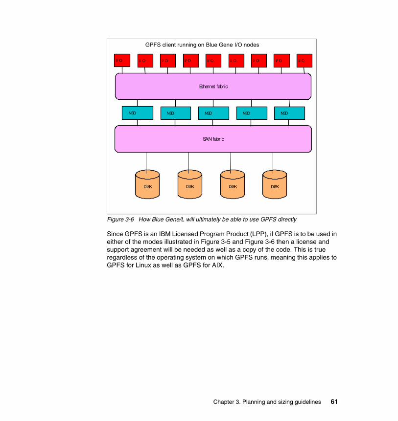
Figure 3-6 How Blue Gene/L will ultimately be able to use GPFS directly

Since GPFS is an IBM Licensed Program Product (LPP), if GPFS is to be used in either of the modes illustrated in Figure 3-5 and Figure 3-6 then a license and support agreement will be needed as well as a copy of the code. This is true regardless of the operating system on which GPFS runs, meaning this applies to GPFS for Linux as well as GPFS for AIX.

3

IBM Research

Blue Gene/L © 2004 IBM Co

DISK DISKDISK DISK

I/ O I/ O I/ O I/ O I/ O I/ O I/ O I/ O I/ O

Ethernet fabric

NSD NSD NSD NSD NSD

SAN fabric

GPFS client running on Blue Gene I/O nodes



Chapter 4. System management

This chapter discusses some of the basic user operations that have to be performed using normal Blue Gene/L usage. Since other materials available (including redbooks) cover the majority of these topics in more detail, we only provide some minimal information needed to start working with and understanding your system. Topics discussed here include:

� Operating your BG/L

� Remote shell

� Monitoring (HW, system SW)

� User environment (variables, directories)

� Scheduling (running) jobs

� Configuration and re-configuration

� Blocks (Partitions)

4


4.1 Operating your BG/LIn this section, we show the basic steps to operate your Blue Gene/L. Since the entire system is composed of multiple nodes playing different roles, an interaction between these is required for allocating partitions, running jobs, and so forth.

4.1.1 Remote shellTo execute commands on I/O nodes and front-end nodes (FEN), some type of remote command execution must be provided. Keep in mind that in the current implementation, there is no out-of-the-box security; thus, if you need to secure your Blue Gene/L system, you need to design the security environment yourself. Generally, it is a good idea to start by establishing some type of boundary firewall around your Blue Gene/L system.

SSH serverThe first step to operate your Blue Gene system is to enable your remote shell. OpenSSH is the default remote shell for SLES9 for the service node (SN) and the front-end nodes. Telnet and rsh are supported in these distributions, but for security reasons, we strongly recommend that you not use these programs. In addition, the default Linux installation does not activate the telnet and rsh servers (telnetd and rshd). For more information on OpenSSH refer to:

http://www.openssh.com/

To check if OpenSSH is installed, log on to both SN and FENs and issue the following commands on the service node and front end nodes:

fumiyasu@rodan:~> rpm -q opensshopenssh-3.4p1-138

To check if the ssh server daemon starts on system boot, issue:

root:~ # chkconfig sshd -asshd 0:off 1:off 2:off 3:on 4:off 5:on 6:off

To check the status, and to start and stop the ssh server, you need to be logged in to the system as user root., then issue the following commands:

root:~ # /etc/init.d/sshd statusChecking for service sshd: running root:~ # /etc/init.d/sshd startStarting SSH daemon doneroot:~ # /etc/init.d/sshd stopShutting down SSH daemon doneroot:~ #



SSH clientThe Linux distributions supported for the Blue Gene/L system have the OpenSSH client installed by default. Check the version to make sure there are no major security issues using the following command:

$ ssh -V OpenSSH_3.9p1, OpenSSL 0.9.7e 25 Oct 2004

If you are using AIX servers connected to your Blue Gene/L environment, you need to check and configure the correct ssh version. Here are some examples:

� For AIX 5L™, you can install it from:

http://www-124.ibm.com/developerworks/projects/opensshi

� For AIX 4.3, you can install it from:

http://www-1.ibm.com/servers/aix/products/aixos/linux/download.html

� For Windows®, there are several ssh clients, for example, PuTTY:

http://www.putty.nl/download.html

For further information about OpenSSH, refer to the following Web site:


Virtual Network Computing (VNC)VNC is a very convenient way to provide Graphical User Interface (GUI) access to remote systems via an IP network connection. Although not supported by IBM, it is a very popular solution for accessing both UNIX and Microsoft® Windows using the GUI desktop.

One of the advantages of using VNC is that even if you lose your connection to the system running the VNC server, all the programs executed in the GUI desktop will continue to run. By reconnecting to your VNC server session, you will be able to continue your work without starting over again.

VNC serverSUSE provides VNC packages in the basic server installation. We recommend that you check the client versions to match the server installed on the machines you want to connect to. You need to set up the VNC server on your service node or front-end nodes.

Note: To check the latest VNC versions and licensing, and for code downloads, see:

http://www.realvnc.com/download.html

Chapter 4. System management 65


http://www-1.ibm.com/servers/aix/products/aixos/linux/download.html





If security is an issue in your environment, you need to set up secure VNC connections. For details, refer to Blue Gene/L: Software Installation, Configuration, and Administration, SG24-6744.

VNC clientYou need to install the VNC client on your workstation to control the server GUI desktop. You can download and install the VNC client for Windows, AIX, Linux, and MacOS from the previously mentioned location.

4.2 Monitoring (HW, system SW)In this section, we describe several methods to monitor your Blue Gene/L system. There are several aspects of monitoring:

1. Blue Gene/L hardware monitoring (nodes, power supplies, thermal status, and so forth)

2. Blue Gene/L software monitoring (CNK, I/O node kernel, jobs, and so forth)

3. Blue Gene/L external elements (SN, FEN, file system servers, and so forth)

This section does not describe monitoring of the external elements, thus you have to consider a way to monitor your SN, FEN, and file system servers. Hardware and system software monitoring are covered by the Midplane Management and Control System (MMCS) and the DB2 databases running on the SN.

For monitoring external elements, we recommend the IBM Cluster System Management (CSM) software. For details about CSM, see:

http://techsupport.services.ibm.com/server/csm

4.2.1 Monitoring logs via the MMCS softwareThe three main components of the MMCS, idoproxydb, mmcs_db_server, and ciodb provide messages about various aspects of the Blue Gene/L system. If you have a VNC session designated as a console on your service node, bglmaster will start all three components, when you connect to the VNC session, in three

Note: Currently there is no off-the-shelf management solution for CSM and Blue Gene/L. Also, currently CSM requires that a separate license be acquired by the customer. There are plans to integrate Blue Gene/L management with CSM, but this solution was in development at the time this redbook was written.



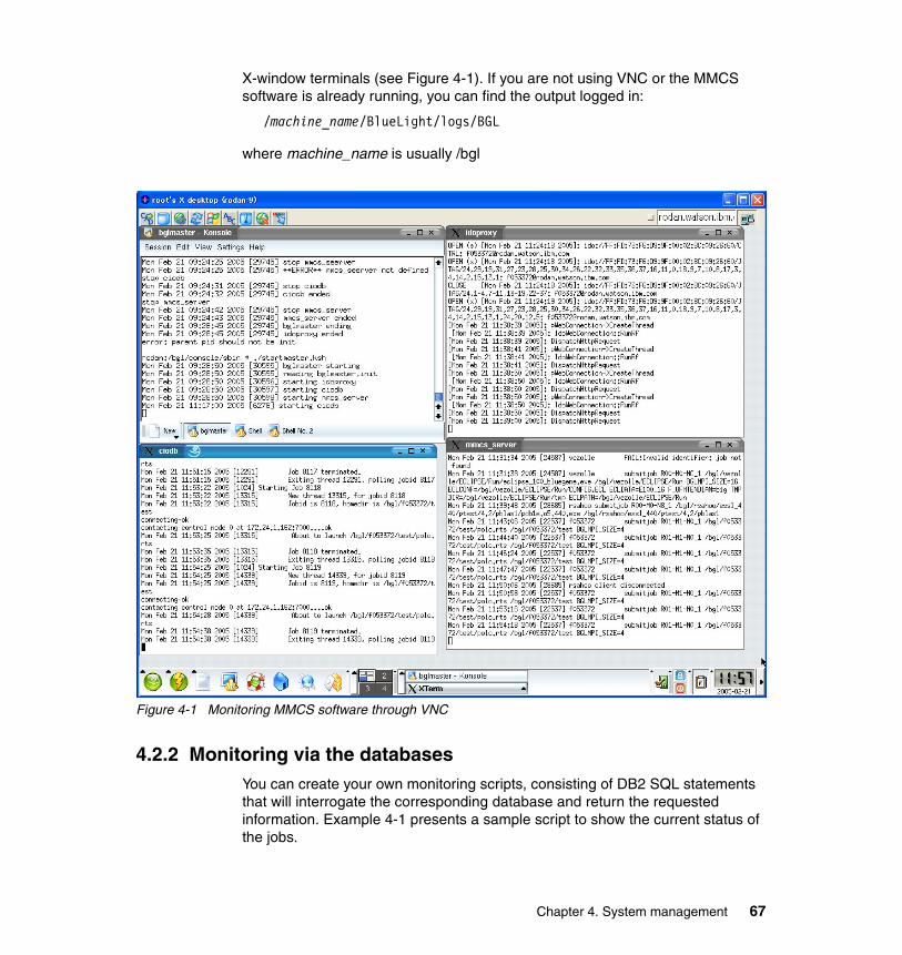
X-window terminals (see Figure 4-1). If you are not using VNC or the MMCS software is already running, you can find the output logged in:

/machine_name/BlueLight/logs/BGL

where machine_name is usually /bgl

Figure 4-1 Monitoring MMCS software through VNC

4.2.2 Monitoring via the databasesYou can create your own monitoring scripts, consisting of DB2 SQL statements that will interrogate the corresponding database and return the requested information. Example 4-1 presents a sample script to show the current status of the jobs.


Example 4-1 Sample script bgljobs

#!/bin/bash

db2 'connect to bgdb0 user bglsysdb using db24bgls'db2 "select jobid,username,blockid,status from bglsysdb.tbgljob"db2 'terminate'

The output of sample script bgljobs looks similar to that shown in Example 4-2.

Example 4-2 Executing the bgljobs script

someone@bgfe01:~> ./bgljobs

Database Connection Information

Database server = DB2/LINUXPPC 8.2.0 SQL authorization ID = BGLSYSDB Local database alias = BGDB0

JOBID USERNAME BLOCKID STATUS----------- -------------------------------- ---------------- ------ 13715 someone R01-M0 R 13716 someone R01-M0 S 13718 someone R01-M0 S 13722 someone R00-M0-NA_1 E 13762 someone R00-M0-NA_1 R 13763 someone R00-M0-NA_1 S

6 record(s) selected.

DB20000I The TERMINATE command completed successfully.someone@bgfe01:~>

Example 4-3 shows an example of listing the tables in the BG/L database.

Example 4-3 List tables in the database

fumiyasu@bgfe02:~> db2(c) Copyright IBM Corporation 1993,2002Command Line Processor for DB2 SDK 8.1.6

You can issue database manager commands and SQL statements from the command prompt. For example: db2 => connect to sample


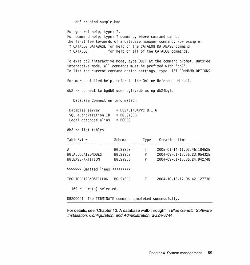
db2 => bind sample.bnd

For general help, type: ?.For command help, type: ? command, where command can bethe first few keywords of a database manager command. For example: ? CATALOG DATABASE for help on the CATALOG DATABASE command ? CATALOG for help on all of the CATALOG commands.

To exit db2 interactive mode, type QUIT at the command prompt. Outside interactive mode, all commands must be prefixed with 'db2'.To list the current command option settings, type LIST COMMAND OPTIONS.

For more detailed help, refer to the Online Reference Manual.

db2 => connect to bgdb0 user bglsysdb using db24bgls



db2 => list tables

Table/View Schema Type Creation time---------------------- ------------- ----- ---------------------------A BGLSYSDB T 2005-01-14-11.07.46.184525BGLALLOCATEDNODES BGLSYSDB V 2004-09-01-15.35.23.954325BGLBASEPARTITION BGLSYSDB V 2004-09-01-15.35.24.942748

>>>>>>> Omitted lines <<<<<<<<<

TBGLTOPDIAGNOSTICLOG BGLSYSDB T 2004-10-12-17.06.42.127730


DB20000I The TERMINATE command completed successfully.

For details, see “Chapter 12. A database walk-through” in Blue Gene/L: Software Installation, Configuration, and Administration, SG24-6744.


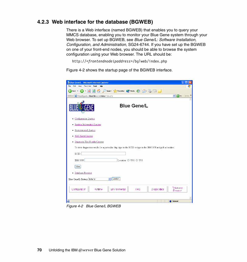
4.2.3 Web interface for the database (BGWEB)There is a Web interface (named BGWEB) that enables you to query your MMCS database, enabling you to monitor your Blue Gene system through your Web browser. To set up BGWEB, see Blue Gene/L: Software Installation, Configuration, and Administration, SG24-6744. If you have set up the BGWEB on one of your front-end nodes, you should be able to browse the system configuration using your Web browser. The URL should be:

http://<frontendnodeipaddress>/bglweb/index.php

Figure 4-2 shows the startup page of the BGWEB interface.

Figure 4-2 Blue Gene/L BGWEB


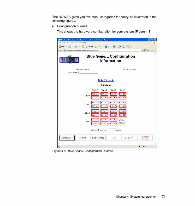
The BGWEB gives you five menu categories for query, as illustrated in the following figures.

� Configuration queries

This shows the hardware configuration for your system (Figure 4-3).

Figure 4-3 Blue Gene/L Configuration Queries


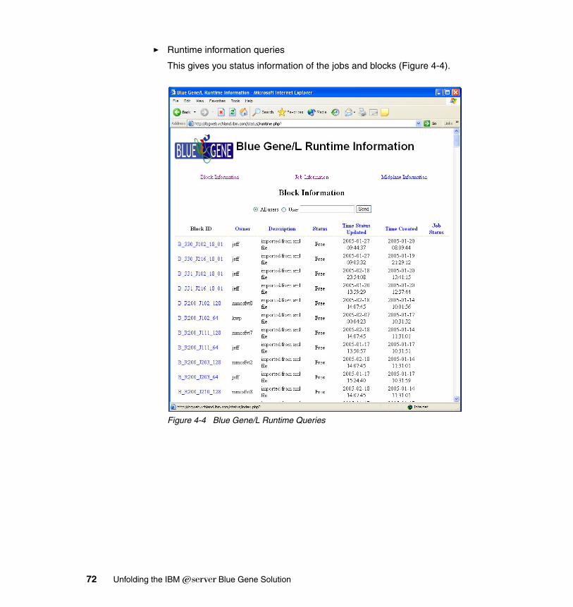
� Runtime information queries

This gives you status information of the jobs and blocks (Figure 4-4).

Figure 4-4 Blue Gene/L Runtime Queries


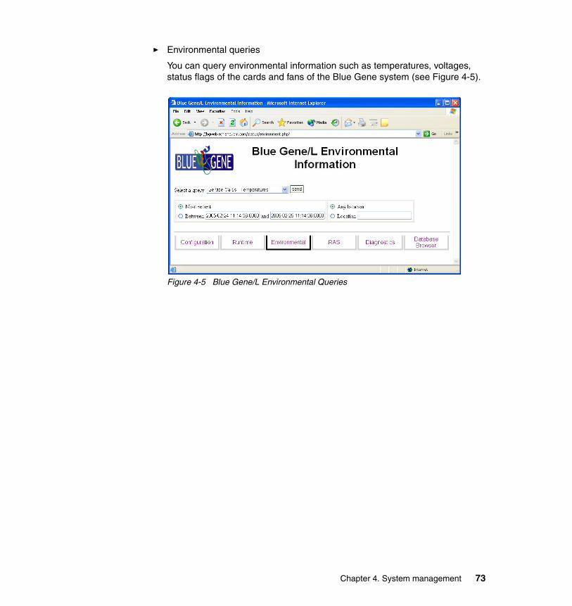
� Environmental queries

You can query environmental information such as temperatures, voltages, status flags of the cards and fans of the Blue Gene system (see Figure 4-5).

Figure 4-5 Blue Gene/L Environmental Queries


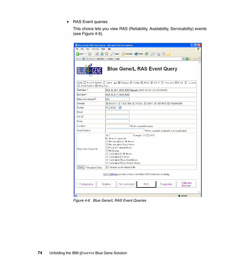
� RAS Event queries

This choice lets you view RAS (Reliability, Availability, Servicability) events (see Figure 4-6).

Figure 4-6 Blue Gene/L RAS Event Queries


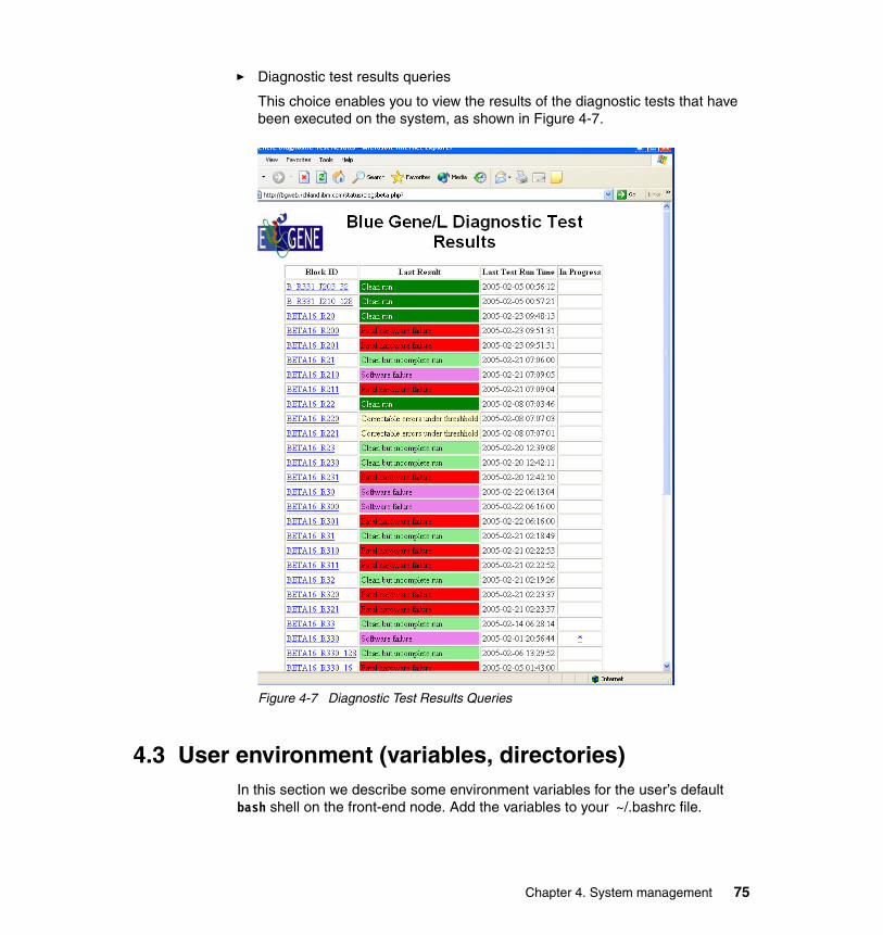
� Diagnostic test results queries

This choice enables you to view the results of the diagnostic tests that have been executed on the system, as shown in Figure 4-7.

Figure 4-7 Diagnostic Test Results Queries

4.3 User environment (variables, directories)In this section we describe some environment variables for the user’s default bash shell on the front-end node. Add the variables to your ~/.bashrc file.


4.3.1 Variables for DB2Add the following variables to set the DB2 environment. You will need these variables (see Example 4-4) in order to use commands that are related to the MMCS (for example, mmcs_db_console, mpirun).

Example 4-4 Adding the variables to your ~/.bashrc file

$ echo “. /bgl/BlueLight/ppcfloor/bglsys/bin/db2profile” >> ~/.bashrc$ echo “export DB_PROPERTY=/bgl/BlueLight/ppcfloor/bglsys/bin/db.properties” \>> ~/.bashrc$ . ~/.bash_profile

Make sure the db2.properties file is configured correctly on your system. A sample file is shown in Example 4-5.

Example 4-5 The db2.properties file

database_name=bgdb0database_user=bglsysdbdatabase_password=db24bglsdatabase_schema_name=bglsysdbmin_pool_connections=2max_pool_connections=30

4.3.2 Variables for MMCSAdd the corresponding variables to export your MMCS server IP address, which should be the same as the service node:

export MMCS_SERVER_IP=<servicenodeipaddress>

The default port for the MMCS server is 32031:

export MMCS_SERVER_PORT=32031

Add the PATH for MMCS software:

PATH=$PATH:/bgl/BlueLight/ppcfloor/bglsys/bin

4.3.3 Variables for MPIRUNYou will need the following variable to use mpirun:

export BRIDGE_CONFIG_FILE=/bgl/BlueLight/ppcfloor/bglsys/bin/bridge.config


The format of the bridge.config file is as follows:

BGL_MACHINE_SN <Machine Serial Number> BGL_MLOADER_IMAGE <Full path to microcode image file> BGL_BLRTS_IMAGE <Full path to compute node run time image file> BGL_LINUX_IMAGE <Full path to linux image file> BGL_RAMDISK_IMAGE <Fill path to ramdisk image file>

Example 4-6 shows a sample of the bridge.config file:

Example 4-6 bridge.config

BGL_MACHINE_SN BGLBGL_MLOADER_IMAGE /bgl/BlueLight/ppcfloor/bglsys/bin/mmcs-mloader.rtsBGL_BLRTS_IMAGE /bgl/BlueLight/ppcfloor/bglsys/bin/rts_hw.rtsBGL_LINUX_IMAGE /bgl/BlueLight/ppcfloor/bglsys/bin/zImage.elfBGL_RAMDISK_IMAGE /bgl/BlueLight/ppcfloor/bglsys/bin/ramdisk.elf

4.3.4 Variables for the compilersExample 4-7 shows the PATH variable pointing to the location of the compilers. You need to change this according to the compiler version you use.

Example 4-7 The compiler path

VAC=/opt/ibmcmp/vac/7.0/binVACPP=/opt/ibmcmp/vacpp/7.0/binXLF=/opt/ibmcmp/XLF/9.1/binPATH=$PATH:$VAC:$VACPP:$XLF

4.3.5 The /bgl directory (the shared file system)All the executables for your programs must reside in the shared file system. For the current implementation this is conventionally NFS mounted on the /bgl directory of the front-end node. If your system’s home directory is not under /bgl, creating one directory with your username is a good idea. This should prevent your work from getting mixed up with that of other users.

4.4 Scheduling (running) jobsThere are several ways to execute a job on the Blue Gene/L system. In this section, we present the ones that are currently available.


4.4.1 MPIRUNMpirun is a program used to run parallel MPI jobs on Blue Gene/L. Mpirun is intended to simplify user interaction with the system by providing a simple common interface for launching, monitoring, and controlling jobs. To use mpirun, make sure your user environment variables are set properly. For further details, refer to 5.3.1, “Using mpirun” on page 107.

4.4.2 IBM LoadLevelerIBM LoadLeveler is a job management system that allows users to run more jobs in less time by matching the jobs' processing needs with the available resources. LoadLeveler schedules jobs, and provides functions for building, submitting, and processing jobs quickly and efficiently in a dynamic environment. More information about LoadLeveler is in 5.5, “Job management” on page 123.

4.4.3 mmcs_db_consoleYou can directly access the Midplane Management and Control System server and run jobsy using mmcs_db_console. For details, refer to Blue Gene/L: Software Installation, Configuration, and Administration, SG24-6744.

Here we show a simple example to run a job using mmcs_db_console.

1. Connect to the mmcs server by using mmcs_db_console.

Example 4-8 Connecting to the mmcs server by mmcs_db_console

fumiyasu@bgfe01:/gsa/watgsa/.home/h1/fumiyasu>. /bgl/BlueLight/ppcfloor/bglsys/bin/db2profilefumiyasu@bgfe01:/gsa/watgsa/.home/h1/fumiyasu> /bgl/BlueLight/ppcfloor/bglsys/bin/mmcs_db_console --consoleip rodan.watson.ibm.com --dbproperties /bgl/console/etc/db.propertiesconnecting to mmcs serverset_username fumiyasuOKconnected to mmcs serverconnected to DB2mmcs$

2. Find a free block using the list_blocks command, which shows allocated blocks.

Example 4-9 Listing free blocks

mmcs$ list_blocksOK


R01-M0 arayshu(0) connectedR01-M1 arayshu(0) connected

3. Allocate a free block using the allocate command.

Example 4-10 Allocating a block

mmcs$ allocate R00-M0OK

4. Submit your job using the submitjob command.

Example 4-11 Submitting job

mmcs$ submitjob R00-M0 /bgl/fumiyasu/helloworld/hello /bgl/fumiyasu/helloworldOKjobId=14174

4.5 Configuration and reconfiguration For the hardware configuration, Blue Gene/L is configured through the discovery process. This is described in more detail in Blue Gene/L: Software Installation, Configuration, and Administration, SG24-6744”.

4.5.1 Configuring system software imagesIf you have to update system software images for you Blue Gene system, you can reconfigure the images using the setblockinfo command, which is one of the mmcs_db_console command (see also Example 4-12).

setblockinfo <blockid> <mloader> <blrts> <linux> <ramdisk>

Example 4-12 example for setblockinfo

mmcs$ setblockinfo M09B_512 /bgl/BlueLight/ppcfloor/bglsys/bin/mmcs_mloader.rts /bgl/BlueLight/ppcfloor/bglsys/bin/rts_hw.rts /bgl/BlueLight/ppcfloor/bglsys/bin/zImage.elf /bgl/BlueLight/ppcfloor/bglsys/bin/ramdisk.elf

4.5.2 Blocks (Partitions)In the context of Blue Gene/L, partition means the same thing as block. It is a set of I/O nodes and compute nodes, called a Pset, which are booted together. The


jobs for Blue Gene/L are executed on blocks (partitions) of nodes. The block is configured from an xml file stored in the DB2 database, using the bpxml2db command under mmcs_db_console.

bpxml2db [path to XML block file] [machinename]

Example 4-13 The blockfile.xml

<BGLBlock name=`R010_J102_128'>

<BGLMidplane midplane=`R010'>

<BGLPset><BGLIONode board=`J102' card=`J18' chip=Ù01'/><BGLComputeNodes board=`J102'/><BGLComputeNodes board=`J104'/><BGLComputeNodes board=`J106'/><BGLComputeNodes board=`J108'/>

<BGLPset>

</BGLMidplane>

<BGLBlock>

For more details, refer to Blue Gene/L: Software Installation, Configuration, and Administration, SG24-6744.


Part 2 BG/L application environment

In this part we describe the parallel application programming environment, general guidelines for application porting, and tuning hints for exploiting the massively parallel structure of Blue Gene/L.

We provide information about the compilers available, and the options you have to use for exploiting the specifics of the system and the CPU design, like the networks available and the double floating point unit.

We summarize the general guidelines you should follow to identify the structure of your application since simple application re-compilation may not create a code which efficiently exploits the massively parallel structure of the system. In other words, we try to identify and classify the characteristics of the applications than need to be considered for efficient running your applications on Blue Gene/L.

Part 2



Chapter 5. Parallel environment

This chapter provides an introduction to the parallel environment available on IBM Eserver Blue Gene Solution for scientific and engineering applications. It presents the fundamentals required to successfully build and run applications on Blue Gene/L.

The following topics are discussed:

� The application development environment

� An introduction to the XL compilers

� Parallel execution environment; needs and requirements to successfully run an application on Blue Gene/L

� Tools that are required to analyze performance and debug applications

� A brief discussion about job management

5

Tip: The “Hello World!” program is used throughout this chapter to illustrate the concepts discussed.


5.1 Application development environmentThroughout this chapter we present our examples based on the fact that the users of the Blue Gene/L system log on to front-end nodes and perform all their work from there. We do not use the IBM LoadLeveler or other high-end job scheduling mechanisms.

The front-end nodes require access to a shared file system that is also connected to the Blue Gene/L I/O nodes.

By convention, this shared file system is mounted at the /bgl mount point. This is not mandatory; it is just done to make different Blue Gene/L system configurations easier to understand, and is the convention adopted for the Blue Gene/L systems used during this project.

The front-end nodes run the SuSE Linux Enterprise Server 9 (SLES 9) operating system platform and should be familiar to existing users of UNIX systems or UNIX-like systems (such as Linux on other hardware platforms).

Every user of the front-end nodes has a separate user environment and logs on with a unique userid/password in the normal way. The user’s home directory may already be defined as part of the shared /bgl file system, but if it is not, the first action users will normally take after logging on is to change to a working directory in the shared file system. Example 5-1 shows this process.

Example 5-1 Logging on to a front-end node

Wed Feb 23 16:23:53 TOT178 ~ > ssh -l jfollows bgfe01.watson.ibm.comPassword: Last login: Wed Feb 23 14:56:50 2005 from jpfthinkpad.itso.ibm.comjfollows@bgfe01:~> cd /bgl/jfollowsjfollows@bgfe01:/bgl/jfollows> lsDLAB hello PMB2.2.1 PMB2.2.1.tar.gz PMB_License.doc sanity

Example 5-1 also shows that the secure shell (ssh) has been used to connect to the front end node. This is not mandatory, but seems advisable, since it avoids the transmission of the userid and password in clear text across the network.

The front end nodes are used to compile code and submit the jobs for Blue Gene/L, and can be used to analyze the results of the jobs once they complete.

It is important to remember two things:

1. Any code and any data files which are needed by the code during execution on the Blue Gene/L system need to be accessible by the Blue Gene/L system, and therefore need to be on the shared file system (/bgl in our environment).


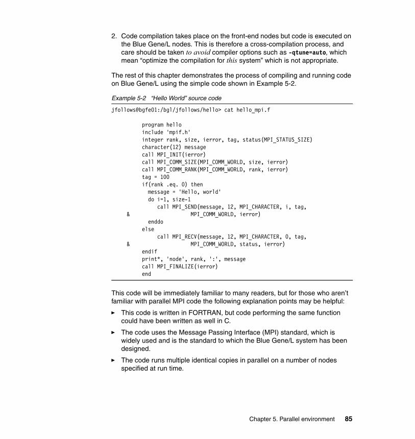
2. Code compilation takes place on the front-end nodes but code is executed on the Blue Gene/L nodes. This is therefore a cross-compilation process, and care should be taken to avoid compiler options such as -qtune=auto, which mean “optimize the compilation for this system” which is not appropriate.

The rest of this chapter demonstrates the process of compiling and running code on Blue Gene/L using the simple code shown in Example 5-2.

Example 5-2 “Hello World” source code

jfollows@bgfe01:/bgl/jfollows/hello> cat hello_mpi.f

program hello include 'mpif.h' integer rank, size, ierror, tag, status(MPI_STATUS_SIZE) character(12) message call MPI_INIT(ierror) call MPI_COMM_SIZE(MPI_COMM_WORLD, size, ierror) call MPI_COMM_RANK(MPI_COMM_WORLD, rank, ierror) tag = 100 if(rank .eq. 0) then message = 'Hello, world' do i=1, size-1 call MPI_SEND(message, 12, MPI_CHARACTER, i, tag, & MPI_COMM_WORLD, ierror) enddo else call MPI_RECV(message, 12, MPI_CHARACTER, 0, tag, & MPI_COMM_WORLD, status, ierror) endif print*, 'node', rank, ':', message call MPI_FINALIZE(ierror) end

This code will be immediately familiar to many readers, but for those who aren’t familiar with parallel MPI code the following explanation points may be helpful:

� This code is written in FORTRAN, but code performing the same function could have been written as well in C.

� The code uses the Message Passing Interface (MPI) standard, which is widely used and is the standard to which the Blue Gene/L system has been designed.

� The code runs multiple identical copies in parallel on a number of nodes specified at run time.

Chapter 5. Parallel environment 85

� When the code runs, each copy determines how many copies are running (“size”) and where in the sequence of identical copies this particular copy is (“rank”).

� One instance of the code running on one of the processors (the one where “rank” equals 0) sends a message to all the other code instances.

� All the other instances of the code receive this message, which is the string “Hello, world”.

� Every code instance prints its value for “rank” followed by the message.

This particular code fragment will probably compile and run without alteration on any parallel supercomputer which supports FORTRAN and MPI.

5.2 XL compilersIn this section we look at the compiler flags that affect the performance of an application, in particular, we emphasize flags that are relevant to Blue Gene/L. This is only a partial list; for a complete list, visit the IBM AIX Compiler information center at:

http://publib.boulder.ibm.com/infocenter/comphelp/index.jsp

In addition, the following books provide information about the compiler: Blue Gene/L: Application Development, SG24-6745, and Advanced POWER Virtualization on IBM eServer p5 Servers, SC24-7940.

A typical example is the property of associativity in a product: at low levels of compiler optimization (for example, -O2), XL FORTRAN will evaluate (a*b*c) always starting from a, even if b*c has already being computed. Although more time will be consumed, it is safer since the answer might be dependent on the order of execution. As the level of optimization increases, some of these restrictions might be eliminated.

5.2.1 Optimization levelA few basic rules to remember when using the compiler for optimization:

� Optimization requires additional compilation time.

Note: It is important to always check answers as you increase the level of compiler optimization. This is due to the fact that the compiler makes certain assumptions about some of the statements in the code that can potentially be optimized by re-writing that section of the code.


� Optimization produces faster code; but you should always check the results, specially when using aggressive levels of compiler optimization.

� By default, the compiler chooses -O0 or -qnoopt.

� Enable compiler optimization with -O[N]; where N is 0, 2, 3, 4, or 5.For example: $xlf -O3

Next, we discuss the different levels of compiler optimization, not to provide an exhaustive list of flags but to convey information about the effects of the so-called performance flags on scientific and engineering applications.

Level 0: -O0This option is recommended for debugging. It is the fastest way to compile the program. It preserves program semantics. This is also useful to see the effect of hand tuning small kernels or certain do loops.

Level 2: -O2This is the same as -O. At this level the compiler performs conservative optimization. The optimization techniques used at this level are:

� Global assignment of user variables to registers, also known as graph coloring register allocation

� Strength reduction and effective use of addressing modes.

� Elimination of redundant instructions, also known as common subexpression elimination

� Elimination of instructions whose results are unused or that cannot be reached by a specified control flow, also known as dead code elimination

� Value numbering (algebraic simplification)

� Movement of invariant code out of loops

� Compile-time evaluation of constant expressions, also known as constant propagation

� Control flow simplification

� Instruction scheduling (reordering) for the target machine

� Loop unrolling and software pipelining

Level 3: -O3At this level the compiler performs more extensive optimization. This includes:

� Deeper inner loop unrolling

� Better loop scheduling


� Increased optimization scope, typically to encompass a whole procedure

� Specialized optimizations (those that might not help all programs)

� Optimizations that require large amounts of compile time or space

� Eliminates implicit memory usage limits (equivalent to compiling with qmaxmem=-1)

� Implies -qnostrict, which allows some reordering of floating-point computations and potential exceptions

Level 4: -O4At this level the compiler introduces more aggressive optimization and increases the optimization scope to the entire program. This option includes:

� -O3

� -qhot

� -qipa

� -qarch=auto

� -qtune=auto

� -qcache=auto

Level 5: -O5At this level the compiler introduces the most aggressive optimization. This option includes:

� -O4

� -qipa=level=2

5.2.2 Machine-specific flagsThis set of flags is specific for a family architecture. The idea is to provide code that is optimized for a particular architecture.

Important: At this level (3), the -qnostrict option is invoked by default. This implies:

� Reordering of floating-point computations

� Reordering or elimination of possible exceptions (for example, division by zero, overflow)

Important: If -O5 is specified on the compile step, then it should be specified on the link step as well.


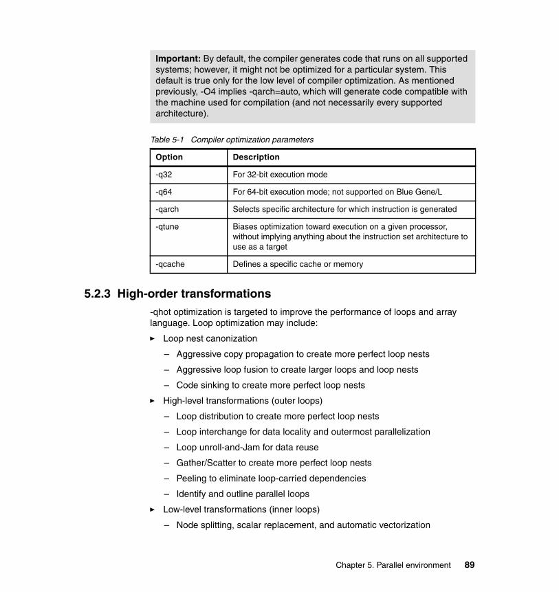
Table 5-1 Compiler optimization parameters

5.2.3 High-order transformations-qhot optimization is targeted to improve the performance of loops and array language. Loop optimization may include:

� Loop nest canonization

– Aggressive copy propagation to create more perfect loop nests

– Aggressive loop fusion to create larger loops and loop nests

– Code sinking to create more perfect loop nests

� High-level transformations (outer loops)

– Loop distribution to create more perfect loop nests

– Loop interchange for data locality and outermost parallelization

– Loop unroll-and-Jam for data reuse

– Gather/Scatter to create more perfect loop nests

– Peeling to eliminate loop-carried dependencies

– Identify and outline parallel loops

� Low-level transformations (inner loops)

– Node splitting, scalar replacement, and automatic vectorization

Important: By default, the compiler generates code that runs on all supported systems; however, it might not be optimized for a particular system. This default is true only for the low level of compiler optimization. As mentioned previously, -O4 implies -qarch=auto, which will generate code compatible with the machine used for compilation (and not necessarily every supported architecture).

Option Description

-q32 For 32-bit execution mode

-q64 For 64-bit execution mode; not supported on Blue Gene/L

-qarch Selects specific architecture for which instruction is generated

-qtune Biases optimization toward execution on a given processor, without implying anything about the instruction set architecture to use as a target

-qcache Defines a specific cache or memory


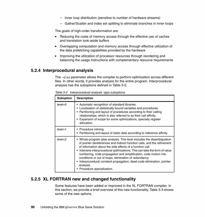
– Inner loop distribution (sensitive to number of hardware streams)

– Gather/Scatter and index set splitting to eliminate branches in inner loops

The goals of high-order transformation are:

� Reducing the costs of memory access through the effective use of caches and translation look-aside buffers

� Overlapping computation and memory access through effective utilization of the data prefetching capabilities provided by the hardware

� Improving the utilization of processor resources through reordering and balancing the usage instructions with complementary resource requirements

5.2.4 Interprocedural analysisThe -qipa parameter allows the compiler to perform optimization across different files. In other words, it provides analysis for the entire program. Interprocedural analysis has the suboptions defined in Table 5-2.

Table 5-2 Interprocedural analysis -qipa suboptions

5.2.5 XL FORTRAN new and changed functionalitySome features have been added or improved in the XL FORTRAN compiler. In this section, we provide a brief overview of this new functionality. Table 5-3 shows some of the new options.

Suboption Description

level=0 • Automatic recognition of standard libraries.• Localization of statistically bound variables and procedures.• Partitioning and layout of procedures according to their calling

relationships, which is also referred to as their call affinity.• Expansion of scope for some optimizations, specially register

allocation.

level=1 • Procedure inlining.• Partitioning and layout of static data according to reference affinity.

level=2 • Whole-program alias analysis. This level includes the disambiguation of pointer dereferences and indirect function calls, and the refinement of information about the side effects of a function call.

• Intensive interprocedural optimizations. This can take the form of value numbering, code propagation and simplification, code motion into conditions or out of loops, elimination of redundancy.

• Interprocedural constant propagation, dead code elimination, pointer analysis.

• Procedure specialization.


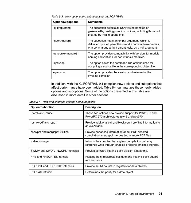
Table 5-3 New options and suboptions for XL FORTRAN

In addition, with the XL FORTRAN 9.1 compiler, new options and suboptions that affect performance have been added. Table 5-4 summarizes these newly added options and suboptions. Some of the options presented in this table are discussed in more detail in other sections.

Table 5-4 New and changed options and suboptions

Option/Suboptions Comments

-qflttrap=nanq The suboption detects all NaN values handled or generated by floating point instructions, including those not created by invalid operations.

-qport=nullarg The suboption treats an empty argument, which is delimited by a left parenthesis and a comma, two commas, or a comma and a right parenthesis, as a null argument.

-qmodule=mangle81 The option provides compatibility with Version 8.1 module naming conventions for non-intrinsic modules.

-qsaveopt The option saves the command-line options used for compiling a source file in the corresponding object file.

-qversion The option provides the version and release for the invoking compiler.

Option/Suboption Description

-qarch and -qtune These two options now provide support for POWER5 and PowerPC 970 architectures (pwr5 and ppc970).

-qshowpdf and -qpdf1 Provide additional call and block count profiling information to an executable.

showpdf and mergepdf utilities Provide enhanced information about PDF-directed compilation; mergepdf merges two or more PDF files.

-qdirecstorage Informs the compiler that a given compilation unit may reference write-through-enabled or cache-inhibited storage.

SWDIV and SWDIV_NOCHK intrinsics Provide software floating-point division algorithms.

FRE and FRSQRTES intrinsic Floating-point reciprocal estimate and floating-point square root reciprocal.

POPCNT and POPCNTB intrinsics Provide set bit counts in registers for data objects.

POPPAR intrinsic Determines the parity for a data object.


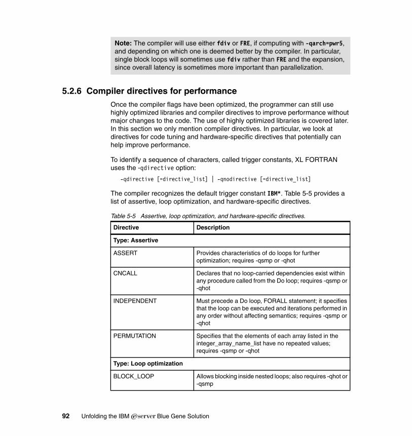
5.2.6 Compiler directives for performanceOnce the compiler flags have been optimized, the programmer can still use highly optimized libraries and compiler directives to improve performance without major changes to the code. The use of highly optimized libraries is covered later. In this section we only mention compiler directives. In particular, we look at directives for code tuning and hardware-specific directives that potentially can help improve performance.

To identify a sequence of characters, called trigger constants, XL FORTRAN uses the -qdirective option:

-qdirective [=directive_list] | -qnodirective [=directive_list]

The compiler recognizes the default trigger constant IBM*. Table 5-5 provides a list of assertive, loop optimization, and hardware-specific directives.

Table 5-5 Assertive, loop optimization, and hardware-specific directives.

Note: The compiler will use either fdiv or FRE, if computing with -qarch=pwr5, and depending on which one is deemed better by the compiler. In particular, single block loops will sometimes use fdiv rather than FRE and the expansion, since overall latency is sometimes more important than parallelization.

Directive Description

Type: Assertive

ASSERT Provides characteristics of do loops for further optimization; requires -qsmp or -qhot

CNCALL Declares that no loop-carried dependencies exist within any procedure called from the Do loop; requires -qsmp or -qhot

INDEPENDENT Must precede a Do loop, FORALL statement; it specifies that the loop can be executed and iterations performed in any order without affecting semantics; requires -qsmp or -qhot

PERMUTATION Specifies that the elements of each array listed in the integer_array_name_list have no repeated values; requires -qsmp or -qhot

Type: Loop optimization

BLOCK_LOOP Allows blocking inside nested loops; also requires -qhot or -qsmp


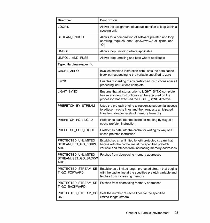
LOOPID Allows the assignment of unique identifier to loop within a scoping unit

STREAM_UNROLL Allows for a combination of software prefetch and loop unrolling; requires -qhot, -qipa=level=2, or -qsmp, and -O4

UNROLL Allows loop unrolling where applicable

UNROLL_AND_FUSE Allows loop unrolling and fuse where applicable

Type: Hardware-specific

CACHE_ZERO Invokes machine instruction dcbz; sets the data cache block corresponding to the variable specified to zero

ISYNC Enables discarding of any prefetched instructions after all preceding instructions complete

LIGHT_SYNC Ensures that all stores prior to LIGHT_SYNC complete before any new instructions can be executed on the processor that executed the LIGHT_SYNC directive

PREFETCH_BY_STREAM Uses the prefetch engine to recognize sequential access to adjacent cache lines and then requests anticipated lines from deeper levels of memory hierarchy

PREFETCH_FOR_LOAD Prefetches data into the cache for reading by way of a cache prefetch instruction

PREFETCH_FOR_STORE Prefetches data into the cache for writing by way of a cache prefetch instruction

PROTECTED_UNLIMITED_STREAM_SET_GO_FORWARD

Establishes an unlimited length protected stream that begins with the cache line at the specified prefetch variable and fetches from increasing memory addresses

PROTECTED_UNLIMITED_STREAM_SET_GO_BACKWARD

Fetches from decreasing memory addresses

PROTECTED_STREAM_SET_GO_FORWARD

Establishes a limited length protected stream that begins with the cache line at the specified prefetch variable and fetches from increasing memory

PROTECTED_STREAM_SET_GO_BACKWARD

Fetches from decreasing memory addresses

PROTECTED_STREAM_COUNT

Sets the number of cache lines for the specified limited-length stream



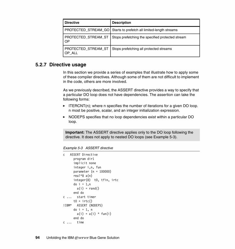
5.2.7 Directive usageIn this section we provide a series of examples that illustrate how to apply some of these compiler directives. Although some of them are not difficult to implement in the code, others are more involved.

As we previously described, the ASSERT directive provides a way to specify that a particular DO loop does not have dependencies. The assertion can take the following forms:

� ITERCNT(n); where n specifies the number of iterations for a given DO loop. n most be positive, scalar, and an integer initialization expression.

� NODEPS specifies that no loop dependencies exist within a particular DO loop.

Example 5-3 ASSERT directive

c ASSERT Directive program dir1 implicit none integer i,n, fun parameter (n = 100000) real*8 a(n) integer(8) t0, tfin, irtc

do i = 1,na(i) = rand()

end doc ... start timer t0 = irtc()!IBM* ASSERT (NODEPS) do i = 1, n a(i) = a(i) * fun(i) end doc ... time

PROTECTED_STREAM_GO Starts to prefetch all limited-length streams

PROTECTED_STREAM_STOP

Stops prefetching the specified protected stream

PROTECTED_STREAM_STOP_ALL

Stops prefetching all protected streams


Important: The ASSERT directive applies only to the DO loop following the directive. It does not apply to nested DO loops (see Example 5-3).


tfin = (irtc() - t0)/1000000 write(6,*)'Time: ',tfin, 'msec.' stop endC function fun(i) fun = i * i return end

In this example we have used the idea of loop-carried dependencies or data dependency. Since this concept is commonly used throughout this chapter, we need to properly define loop-carried dependencies:

Dependencies Current iteration requires data computed in some previous iteration, or computes data for some subsequent iteration.

An example may be seen in a loop with, a(i) = a(i-1)*2, computing a(5) requires a(4).

The loop optimization directive is BLOCK_LOOP. This directive relies on a well known optimization technique called blocking. This directive separates large iterations into smaller groups of iterations. Hence, the name blocking. The basic idea is to increase the utilization of the submemory hierarchy. Notice that in Example 5-4, L2_cache_size and L3_cache_size need to be assigned values corresponding to the cache of the particular system where this example is going to be executed.

Example 5-4 BLOCK_LOOP directive

c BLOCK_LOOP Directive program dir4 implicit none integer i,j,k,n integer L3_cache_size, L3_cache_block integer L2_cache_size, L2_cache_block parameter (n = 100) integer a(n,n), b(n,n), c(n,n) integer(8) t0, tfin, irtc do j = 1,n do i = 1,n a(i,j) = rand() b(i,j) = rand() enddo enddo do j = 1, n do i = 1, n


c(i,j)=0.0 enddo enddoc ... start timer t0 = irtc()!IBM* BLOCK_LOOP(L3_cache_size, L3_cache_block) do i = 1, n

!IBM* LOOPID(L3_cache_block)!IBM* BLOCK_LOOP(L2_cache_size, L2_cache_block) do j = 1, n

!IBM* LOOPID(L2_cache_block) do k = 1, n c(i,j) = c(i,j) + a(i,k) * b(k,j) enddo enddo enddOc ... time tfin = (irtc() - t0)/1000000 write(6,*)'Time: ',tfin, 'msec.' call dummy (c,n) stop endc

5.2.8 Blue Gene/L compiler featuresAlthough Blue Gene/L uses the IBM XL compilers, there are differences with respect to all other IBM servers. In particular, in the case of the IBM pSeries Linux programming model, some of the differences from Linux PPC64 are:

� No stdin

� No asynchronous I/O

� No dynamic linking

� No demand paging/swap

– Virtual address space is mapped 1-on-1 with physical memory

� No read-only memory

– Due to CNK design decision

– No SIGSEGV writing to a const char *p

Also, certain system calls are not supported; they are identified in this book and in Blue Gene/L: Application Development, SG24-6745. We do cover some of the system calls that are supported with limitations.


On Blue Gene/L the front end is running SuSE SLES9 Linux/PPC64 and it provides the platform for IBM XL cross compilers for Blue Gene/L. The cross-compiler environment can be summarized by indicating the following components that are required:

� Front-end node running SuSE SLES 9 on a PPC64

� PowerPC-Linux-GNU to generate PowerPC-blrts-GNU

� GNU toolchain for Blue Gene/L

� IBM XL cross compilers for Blue Gene/L

Currently, to build binaries or executables for Blue Gene/L, the IBM XL compilers require the following:

� Installation of IBM XLC V7.0/XLF V9.1 compilers for SuSE SLES9 Linux/PPC64

� Installation of the Blue Gene/L add-on that includes Blue Gene/L versions of the XL run-time libraries, compiler scripts, and configuration files.

– The GNU Blue Gene/L toolchain is required.

• gcc, g++, and g77 v3.2

• binutils (as, ld, ... ) v2.13

• GLIBC v2.2.5

– Blue Gene/L support supplied via patches. The customer applies the patches and builds the toolchain; IBM supplies scripts to download, patch, and build everything.

As mentioned, on Blue Gene/L we need to include an add-on as part of the compiler. Figure 5-1 and Figure 5-2 illustrate the different levels of libraries that interact with the kernel.


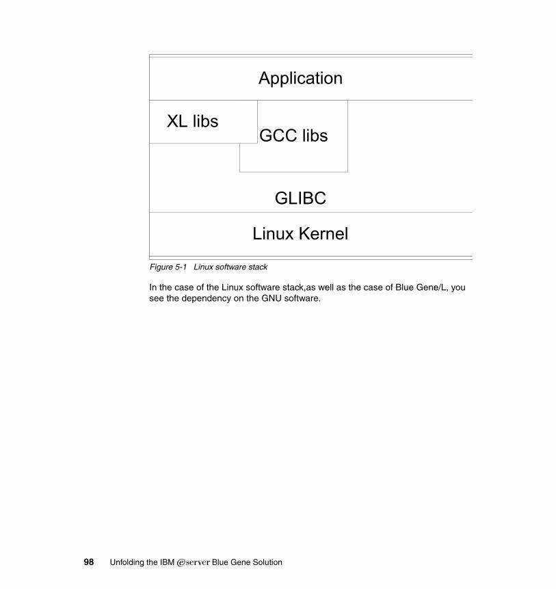
Figure 5-1 Linux software stack

In the case of the Linux software stack,as well as the case of Blue Gene/L, you see the dependency on the GNU software.

GLIBC

Application

GCC libsXL libs

Linux Kernel


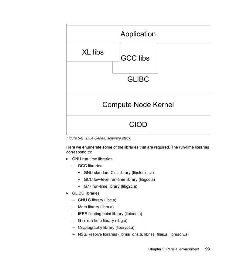
Figure 5-2 Blue Gene/L software stack.

Here we enumerate some of the libraries that are required. The run-time libraries correspond to:

� GNU run-time libraries

– GCC libraries

• GNU standard C++ library (libstdc++.a)

• GCC low-level run-time library (libgcc.a)

• G77 run-time library (libg2c.a)

� GLIBC libraries

– GNU C library (libc.a)

– Math library (libm.a)

– IEEE floating point library (libieee.a)

– G++ run-time library (libg.a)

– Cryptography library (libcrypt.a)

– NSS/Resolve libraries (libnss_dns.a, libnss_files.a, libresolv.a)

GLIBC

Application

GCC libsXL libs

CIOD

Compute Node Kernel


� IBM XL run-time libraries

– IBM C++ library (libibmc++.a)

• Very light wrapper to libstdc++.a

– IBM XLF run-time library (libxlf90.a)

– IBM XL low-level run-time library (libxl.a)

– IBM XL optimized intrinsic library (libxlopt.a)

• Vector intrinsic functions

• BLASS routines

– IBM XL MASSV library (libmassv.a)

• Vector intrinsic functions

– IBM XL OpenMP compatibility library (libxlomp_ser.a)

This gives us a set of two working compilers in the front-end:

� Linux: xlc, xlC, xlf, xlf90, and so forth

� Blue Gene/L: blrts_xlc, blrts_xlC, blrts_xlf, blrts_xlf90, and so forth

We also mentioned that the Blue Gene/L add-on requires compiler scripts. Example 5-5 illustrates one of the current scripts.

Example 5-5 Compiler wrapper

#!/bin/bash

export XL_CONFIG=ècho ${0} | sed -e 's#/opt/ibmcmp/.*$#/etc/opt/ibmcmp/#'``basename ${0%_*}`.cfgblrtscmd="`dirname ${0%_*}`/${0##*_} $@"

if [ -n "$BLRTSDEBUG" ]; then echo "export XL_CONFIG=${XL_CONFIG}" echo "$blrtscmd"fi

This script takes the blrts_xl* and removes the blrts_ to get xl*. It then executes xl* with the XL_CONFIG environment variable pointing to a particular Blue Gene/L configuration file so it links against a particular XL and GNU libraries. It also adds -qbgl and other options to every compile command so as to turn it into a Blue Gene/L cross compiler.


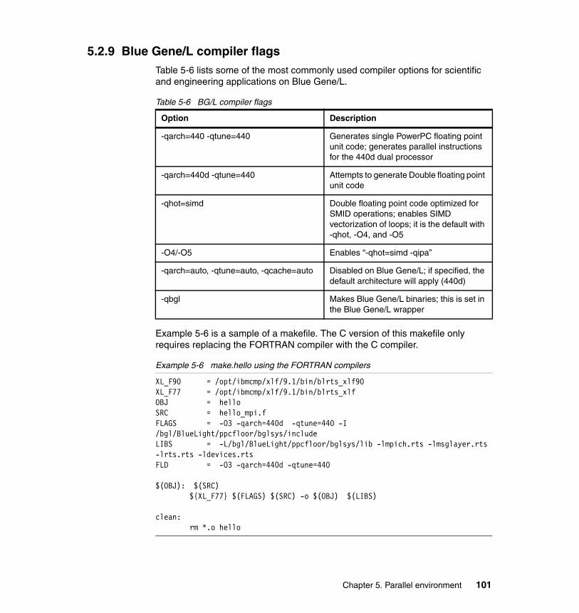
5.2.9 Blue Gene/L compiler flagsTable 5-6 lists some of the most commonly used compiler options for scientific and engineering applications on Blue Gene/L.

Table 5-6 BG/L compiler flags

Example 5-6 is a sample of a makefile. The C version of this makefile only requires replacing the FORTRAN compiler with the C compiler.

Example 5-6 make.hello using the FORTRAN compilers

XL_F90 = /opt/ibmcmp/xlf/9.1/bin/blrts_xlf90XL_F77 = /opt/ibmcmp/xlf/9.1/bin/blrts_xlfOBJ = helloSRC = hello_mpi.fFLAGS = -O3 -qarch=440d -qtune=440 -I /bgl/BlueLight/ppcfloor/bglsys/includeLIBS = -L/bgl/BlueLight/ppcfloor/bglsys/lib -lmpich.rts -lmsglayer.rts -lrts.rts -ldevices.rtsFLD = -O3 -qarch=440d -qtune=440

$(OBJ): $(SRC) ${XL_F77} $(FLAGS) $(SRC) -o $(OBJ) $(LIBS)

clean: rm *.o hello

Option Description

-qarch=440 -qtune=440 Generates single PowerPC floating point unit code; generates parallel instructions for the 440d dual processor

-qarch=440d -qtune=440 Attempts to generate Double floating point unit code

-qhot=simd Double floating point code optimized for SMID operations; enables SIMD vectorization of loops; it is the default with -qhot, -O4, and -O5

-O4/-O5 Enables “-qhot=simd -qipa”

-qarch=auto, -qtune=auto, -qcache=auto Disabled on Blue Gene/L; if specified, the default architecture will apply (440d)

-qbgl Makes Blue Gene/L binaries; this is set in the Blue Gene/L wrapper


5.3 Parallel execution environmentNow that we have successfully compiled code for Blue Gene/L, how does the code actually run?

Blue Gene/L is designed to run code which uses MPI. MPI is the Message Passing Interconnect standard used for communication between distinct and separate parallel tasks. The actual number of parallel tasks is chosen when the job is run, not when the code is compiled.

So, the first decision which needs to be made is: How many parallel tasks do we want for a particular job run?

Having decided on the number of tasks, it is necessary to allocate a Blue Gene/L partition that contains sufficient compute nodes to run the job. The size of partitions available to users of Blue Gene/L are determined by the system administrators, so an exact match may not be possible, in which case it is necessary to allocate a partition with more compute nodes than are actually required.

Some of the documents and certain commands refer to a Blue Gene/L block. The terms block and partition are interchangeable.

Each partition also includes at least one Blue Gene/L I/O node. This I/O node is required. Without it, communication between the compute nodes and the external file system is not possible.

Important: In the default configuration, Communication Coprocessor Mode, each Blue Gene/L compute node runs a single MPI task, which has access to 512MB of memory. In Virtual Node Mode, each Blue Gene/L compute node runs two MPI tasks, one task per processor, each task having access to 256MB of memory.

Note: The current implementation (no LoadLeveler), requires that a partition be allocated explicitly prior to submitting a job for execution. When LoadLeveler support is available, LoadLeveler manages the partition allocation automatically prior to submitting the job for execution in that partition.

The mpirun command can also be used to allocate a partition and run a job in a single command, but currently the smallest size partition which can be allocated is a midplane (512 nodes / 1024 CPUs).


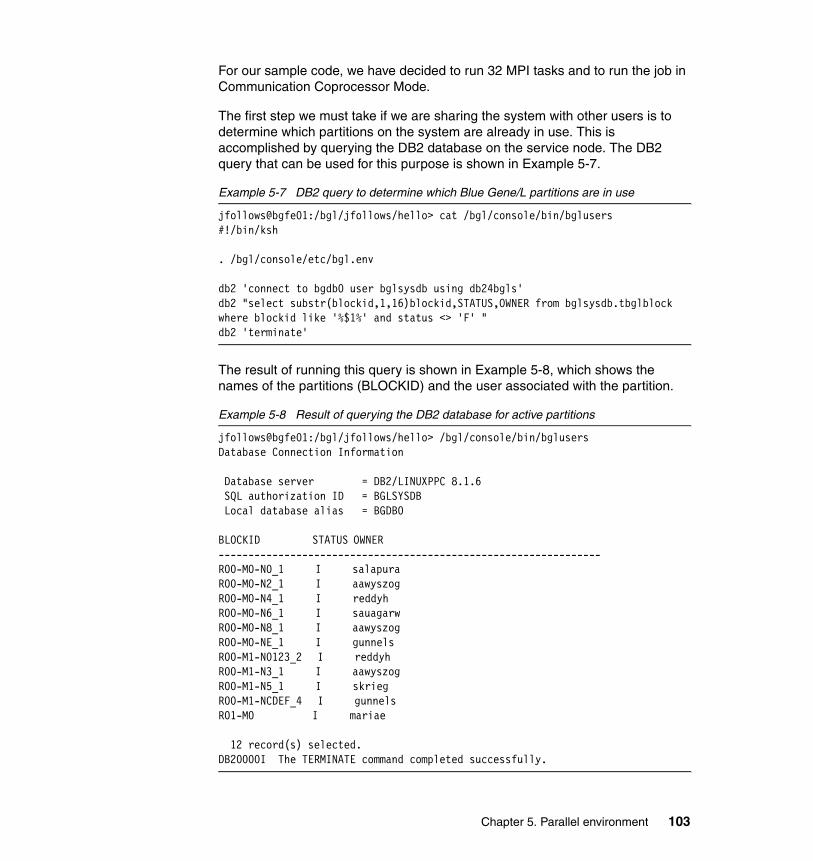
For our sample code, we have decided to run 32 MPI tasks and to run the job in Communication Coprocessor Mode.

The first step we must take if we are sharing the system with other users is to determine which partitions on the system are already in use. This is accomplished by querying the DB2 database on the service node. The DB2 query that can be used for this purpose is shown in Example 5-7.

Example 5-7 DB2 query to determine which Blue Gene/L partitions are in use

jfollows@bgfe01:/bgl/jfollows/hello> cat /bgl/console/bin/bglusers#!/bin/ksh

. /bgl/console/etc/bgl.env

db2 'connect to bgdb0 user bglsysdb using db24bgls'db2 "select substr(blockid,1,16)blockid,STATUS,OWNER from bglsysdb.tbglblock where blockid like '%$1%' and status <> 'F' "db2 'terminate'

The result of running this query is shown in Example 5-8, which shows the names of the partitions (BLOCKID) and the user associated with the partition.

Example 5-8 Result of querying the DB2 database for active partitions

jfollows@bgfe01:/bgl/jfollows/hello> /bgl/console/bin/bglusersDatabase Connection Information


BLOCKID STATUS OWNER ----------------------------------------------------------------R00-M0-N0_1 I salapura R00-M0-N2_1 I aawyszog R00-M0-N4_1 I reddyh R00-M0-N6_1 I sauagarw R00-M0-N8_1 I aawyszog R00-M0-NE_1 I gunnels R00-M1-N0123_2 I reddyh R00-M1-N3_1 I aawyszog R00-M1-N5_1 I skrieg R00-M1-NCDEF_4 I gunnels R01-M0 I mariae

12 record(s) selected.DB20000I The TERMINATE command completed successfully.


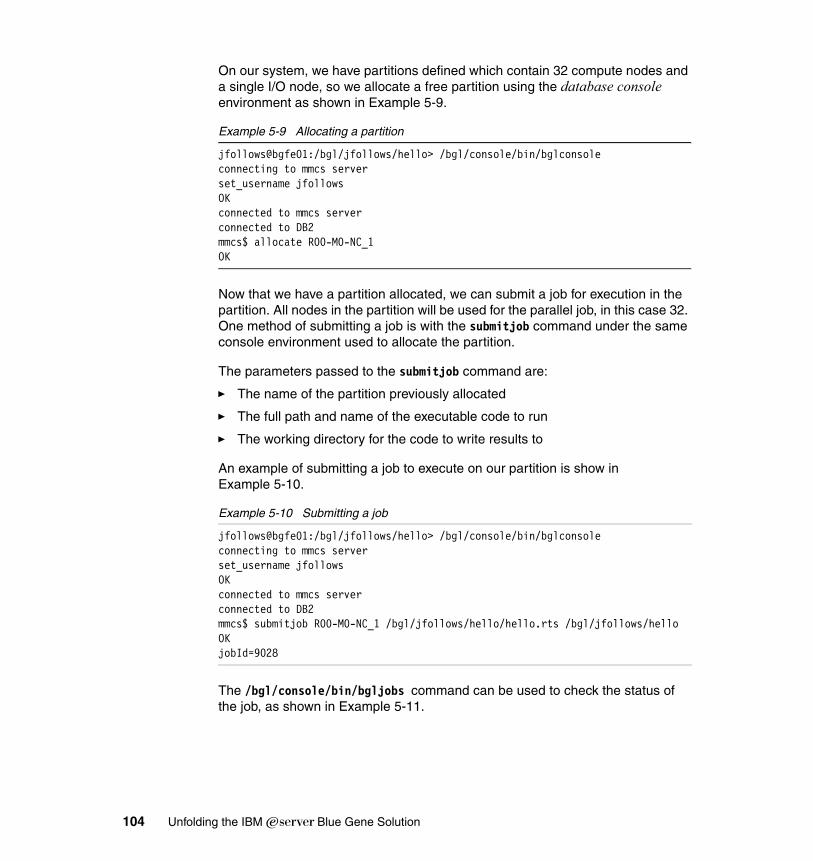
On our system, we have partitions defined which contain 32 compute nodes and a single I/O node, so we allocate a free partition using the database console environment as shown in Example 5-9.

Example 5-9 Allocating a partition

jfollows@bgfe01:/bgl/jfollows/hello> /bgl/console/bin/bglconsoleconnecting to mmcs serverset_username jfollowsOKconnected to mmcs serverconnected to DB2mmcs$ allocate R00-M0-NC_1OK

Now that we have a partition allocated, we can submit a job for execution in the partition. All nodes in the partition will be used for the parallel job, in this case 32. One method of submitting a job is with the submitjob command under the same console environment used to allocate the partition.

The parameters passed to the submitjob command are:

� The name of the partition previously allocated

� The full path and name of the executable code to run

� The working directory for the code to write results to

An example of submitting a job to execute on our partition is show in Example 5-10.

Example 5-10 Submitting a job

jfollows@bgfe01:/bgl/jfollows/hello> /bgl/console/bin/bglconsoleconnecting to mmcs serverset_username jfollowsOKconnected to mmcs serverconnected to DB2mmcs$ submitjob R00-M0-NC_1 /bgl/jfollows/hello/hello.rts /bgl/jfollows/helloOKjobId=9028

The /bgl/console/bin/bgljobs command can be used to check the status of the job, as shown in Example 5-11.


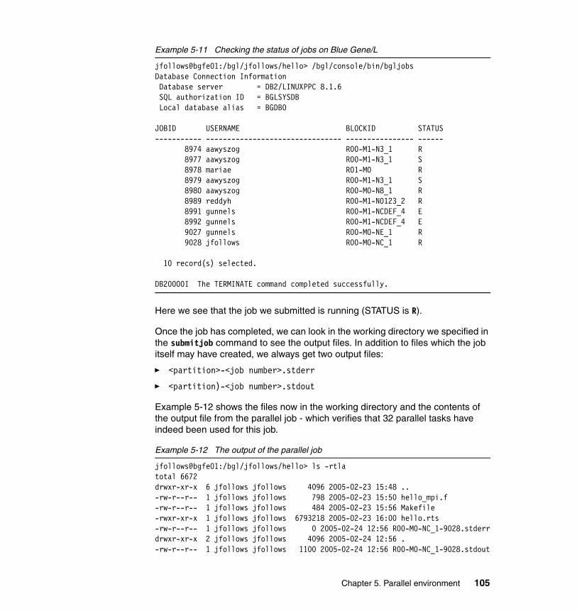
Example 5-11 Checking the status of jobs on Blue Gene/L

jfollows@bgfe01:/bgl/jfollows/hello> /bgl/console/bin/bgljobsDatabase Connection InformationDatabase server = DB2/LINUXPPC 8.1.6 SQL authorization ID = BGLSYSDB Local database alias = BGDB0

JOBID USERNAME BLOCKID STATUS----------- -------------------------------- ---------------- ------ 8974 aawyszog R00-M1-N3_1 R 8977 aawyszog R00-M1-N3_1 S 8978 mariae R01-M0 R 8979 aawyszog R00-M1-N3_1 S 8980 aawyszog R00-M0-N8_1 R 8989 reddyh R00-M1-N0123_2 R 8991 gunnels R00-M1-NCDEF_4 E 8992 gunnels R00-M1-NCDEF_4 E 9027 gunnels R00-M0-NE_1 R 9028 jfollows R00-M0-NC_1 R



Here we see that the job we submitted is running (STATUS is R).

Once the job has completed, we can look in the working directory we specified in the submitjob command to see the output files. In addition to files which the job itself may have created, we always get two output files:

� <partition>-<job number>.stderr

� <partition)-<job number>.stdout

Example 5-12 shows the files now in the working directory and the contents of the output file from the parallel job - which verifies that 32 parallel tasks have indeed been used for this job.

Example 5-12 The output of the parallel job

jfollows@bgfe01:/bgl/jfollows/hello> ls -rtlatotal 6672drwxr-xr-x 6 jfollows jfollows 4096 2005-02-23 15:48 ..-rw-r--r-- 1 jfollows jfollows 798 2005-02-23 15:50 hello_mpi.f-rw-r--r-- 1 jfollows jfollows 484 2005-02-23 15:56 Makefile-rwxr-xr-x 1 jfollows jfollows 6793218 2005-02-23 16:00 hello.rts-rw-r--r-- 1 jfollows jfollows 0 2005-02-24 12:56 R00-M0-NC_1-9028.stderrdrwxr-xr-x 2 jfollows jfollows 4096 2005-02-24 12:56 .-rw-r--r-- 1 jfollows jfollows 1100 2005-02-24 12:56 R00-M0-NC_1-9028.stdout


jfollows@bgfe01:/bgl/jfollows/hello> cat R00-M0-NC_1-9028.stdout stdout[3]: node 3 :Hello, worldstdout[23]: node 23 :Hello, worldstdout[0]: node 0 :Hello, worldstdout[1]: node 1 :Hello, worldstdout[29]: node 29 :Hello, worldstdout[6]: node 6 :Hello, worldstdout[2]: node 2 :Hello, worldstdout[4]: node 4 :Hello, worldstdout[7]: node 7 :Hello, worldstdout[10]: node 10 :Hello, worldstdout[5]: node 5 :Hello, worldstdout[14]: node 14 :Hello, worldstdout[16]: node 16 :Hello, worldstdout[17]: node 17 :Hello, worldstdout[20]: node 20 :Hello, worldstdout[19]: node 19 :Hello, worldstdout[30]: node 30 :Hello, worldstdout[11]: node 11 :Hello, worldstdout[8]: node 8 :Hello, worldstdout[9]: node 9 :Hello, worldstdout[15]: node 15 :Hello, worldstdout[12]: node 12 :Hello, worldstdout[13]: node 13 :Hello, worldstdout[27]: node 27 :Hello, worldstdout[28]: node 28 :Hello, worldstdout[31]: node 31 :Hello, worldstdout[18]: node 18 :Hello, worldstdout[21]: node 21 :Hello, worldstdout[22]: node 22 :Hello, worldstdout[24]: node 24 :Hello, worldstdout[25]: node 25 :Hello, worldstdout[26]: node 26 :Hello, world

Jobs can be run in Virtual Node Mode if the partition in which they run is initialized in this mode. In our case, we can free the partition we have just created and re-allocate it in this mode, as shown in Example 5-13.

Example 5-13 Re-allocating a partition using Virtual Node Mode

jfollows@bgfe01:/bgl/jfollows/hello> /bgl/console/bin/bglconsoleconnecting to mmcs serverset_username jfollowsOKconnected to mmcs serverconnected to DB2


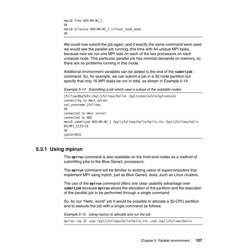
mmcs$ free R00-M0-NC_1OKmmcs$ allocate R00-M0-NC_1 virtual_node_modeOK

We could now submit the job again, and if exactly the same command were used we would see the parallel job running, this time with 64 unique MPI tasks, because now we run one MPI task on each of the two processors on each compute node. This particular parallel job has minimal demands on memory, so there are no problems running in this mode.

Additional environment variables can be added to the end of the submitjob command. So, for example, we can submit a job in a 32-node partition but specify that only 16 MPI tasks be run in total, as shown in Example 5-14.

Example 5-14 Submitting a job which uses a subset of the available nodes

jfollows@bgfe01:/bgl/jfollows/hello> /bgl/console/bin/bglconsoleconnecting to mmcs serverset_username jfollowsOKconnected to mmcs serverconnected to DB2mmcs$ submitjob R00-M0-NC_1 /bgl/jfollows/hello/hello.rts /bgl/jfollows/hello BGLMPI_SIZE=16OKjobId=9031

5.3.1 Using mpirunThe mpirun command is also available on the front-end nodes as a method of submitting jobs to the Blue Gene/L processors.

The mpirun command will be familiar to existing users of supercomputers that implement MPI using mpich, just as Blue Gene/L does, such as Linux clusters.

The use of the mpirun command offers one clear usability advantage over submitjob because mpirun allows the allocation of the partition and the execution of the parallel job to be performed through a single command.

So, for our “Hello, world” job it would be possible to allocate a 32-CPU partition and to execute the job with a single command as follows:

Example 5-15 Using mpirun to allocate and run the job

mpirun -np 32 -exe /bgl/jfollows/hello/hello.rts -cwd /bgl/jfollows/hello


The previous command specifies the number of processors but places no requirement on the layout of the processors. A new partition will be created which contains the appropriate number of processors and the job is then submitted to execute in that partition.

Alternatively, mpirun can be used to create a partition with a particular layout (or shape). In this case, instead of specifying the total number of processors, the shape of the partition is specified, as shown in Example 5-16.

Example 5-16 Using mpirun to run a job in a partition with a given shape

mpirun -shape 4x4x2 -exe /bgl/jfollows/hello/hello.rts -cwd /bgl/jfollows/hello

If we know the shape of the partition, we may be able to take advantage of this knowledge in tuning the application; this is discussed further in 5.3.2, “Mapping MPI tasks to Blue Gene/L nodes” on page 109.

To use Virtual Node Mode, an extra parameter is added to the mpirun command, as shown in Example 5-17.

Example 5-17 Using mpirun to run a job in Virtual Node Mode

mpirun -np 32 -mode VN -exe /bgl/jfollows/hello/hello.rts -cwd \ /bgl/jfollows/hello

The shape and np options can be used together, in which case the shape specification determines the size of the partition, and the number of processors can be equal to or less than the number available in the partition. Using mpirun to achieve the same result as shown in Example 5-17, where we ran the parallel job on 16 processors in a partition which comprised 32 processors, we would use the command such as shown in Example 5-18.

Example 5-18 Using mpirun to run a job on a subset of nodes in a partition

mpirun -shape 4x4x2 -np 16 -exe /bgl/jfollows/hello/hello.rts -cwd \ /bgl/jfollows/hello

Here the partition comprises 32 processors, but we are only running the parallel job on 16 of the processors in the partition.

Finally, mpirun still provides the option of allocating a partition in advance of job submission. In this case, in a similar method as for the submitjob command shown in Example 5-14 on page 107, we can submit a job to run on an existing partition using mpirun as shown in Example 5-19.


Example 5-19 Using mpirun to run a job in an existing partition

mpirun -partition=R00-M0-NC_1 -exe /bgl/jfollows/hello/hello.rts -cwd \ /bgl/jfollows/hello

When specifying an existing partition, mpirun will ignore any shape specification on the command, but the number of processors to be used can still be specified (of course, provided that the number of processors is less than or equal to the number available in the partition).

5.3.2 Mapping MPI tasks to Blue Gene/L nodes

In Example 5-12 on page 105 we showed the output of a parallel job. We used the submitjob command to run our parallel code “hello.rts” as shown in Example 5-15 on page 107, and because the partition we allocated had 32 compute nodes, the result was that 32 instances of the same executable code ran in parallel.

All the compute nodes in the Blue Gene/L system are identical; they all have the same amount of memory, run the same processor, and have the same number and type of connections to other nodes in the cluster.

Just as for other cluster types, the location of a particular compute node in relation to all other compute nodes in the cluster may be important.

For example, in a cluster made from multiple 32-way SMP systems, a task running on a particular processor in the cluster will probably have higher bandwidth and lower latency when communicating with another task running on the same SMP system as when communicating with a task running on a different SMP system. This can lead to strategies of MPI and code design maximizing total performance by understanding the topology of the MPI tasks and how they relate to each other. For example, an enhanced collective operation may have a single MPI task perform all communication with MPI tasks on remote systems.

Similar considerations apply to Blue Gene/L. One strategy is to maximize communication between tasks which are more close to each other and minimize communication between tasks which are less close to each other. In this case, we define closeness as being the number of steps through the communication

Note: This section goes into a lot of detail about how some aspects of Blue Gene/L really work. It’s not necessary to understand this level of detail just to run jobs on Blue Gene/L, but ultimately anyone wanting to do serious performance tuning is going to have to understand this material.


network between a pair of tasks, observing that on Blue Gene/L this can vary tremendously.

Section 2.1.6, “Communications” on page 19 describes the networks that connect the Blue Gene/L nodes to each other. The rest of this section considers the torus network, which is used for the majority of the MPI communication.

For each partition, the compute nodes that form part of the partition are laid out as a subset of the complete Blue Gene/L torus network in a three dimensional mesh, such as shown in Figure 2-3 on page 20. For a particular parallel job, how can we relate the rank of a particular instance of the code (which is a positive integer starting at zero, used as shown in Example 5-2 on page 85) to its position relative to the other code instances on the torus network?

It turns out that there are three ways of positioning the individual MPI tasks across a given torus network:

1. A default automatic allocation strategy

2. An alternative automatic allocation strategy

3. Explicitly mapping each individual MPI tasks to a specific location

To understand these options, begin by considering a mesh similar to the one shown in Figure 2-3 on page 20, but instead of a 3x3x3 mesh we need to consider one that represents a complete Blue Gene/L partition. The smallest partition we can allocate on our Blue Gene/L system is one with 32 compute nodes and a single I/O node. For the purposes of this section we are only interested in the compute nodes and their layout on the mesh.

Consider each position on the mesh is represented by three dimensional Cartesian coordinates X, Y, and Z. Consider the node at one corner of the mesh (maybe think about this as the bottom left of the mesh) as having coordinates X=0, Y=0, Z=0. Let us represent this node as having coordinate representation (0,0,0). Note that it has only three connections to other cubes in the mesh:

1. To its right in the figure, to the cube with coordinates X=1, Y=0, Z=0 (1,0,0)

2. Above it in the figure, to the cube with coordinates X=0, Y=1, Z=0 (0,1,0)

3. Behind it in the figure, to the cube with coordinates X=0, Y=0, Z=1 (0,0,1)

Note: This is the difference between a mesh and a torus. In a torus configuration on Blue Gene/L each node has six connections to its neighbor nodes. In a mesh, some nodes on the edges of the mesh have fewer connections. A Blue Gene/L partition may or may not have a torus topology. On our small partition with 32 nodes we only have a mesh, not a full torus.


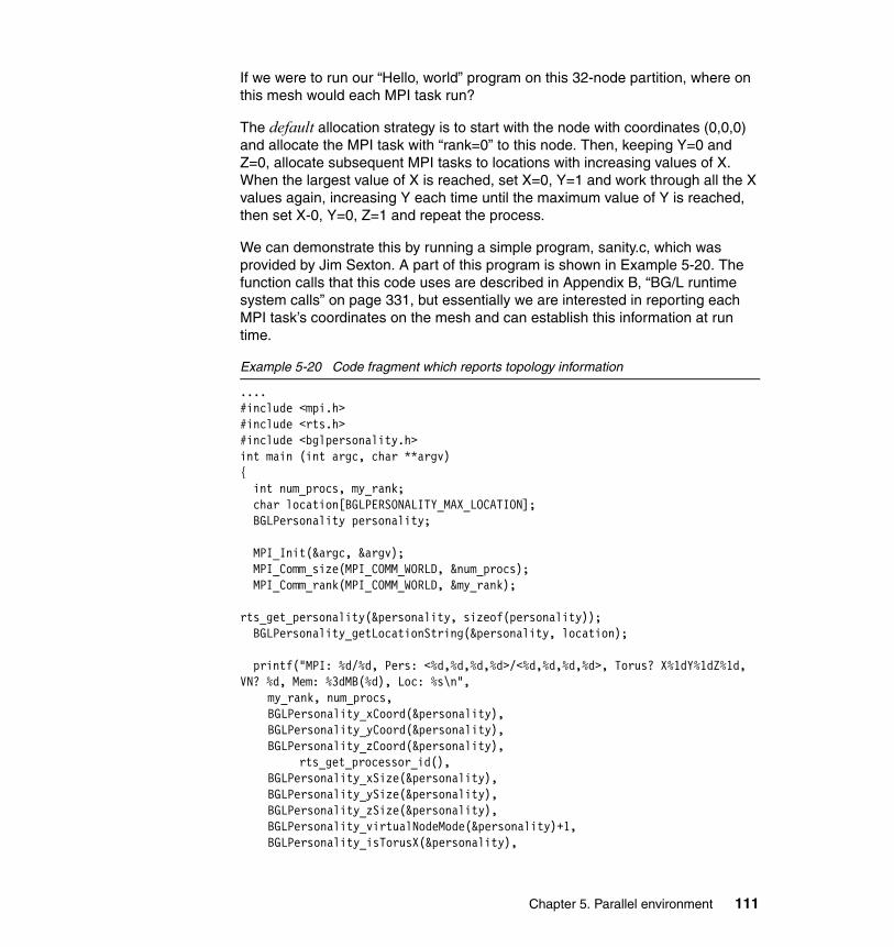
If we were to run our “Hello, world” program on this 32-node partition, where on this mesh would each MPI task run?

The default allocation strategy is to start with the node with coordinates (0,0,0) and allocate the MPI task with “rank=0” to this node. Then, keeping Y=0 and Z=0, allocate subsequent MPI tasks to locations with increasing values of X. When the largest value of X is reached, set X=0, Y=1 and work through all the X values again, increasing Y each time until the maximum value of Y is reached, then set X-0, Y=0, Z=1 and repeat the process.

We can demonstrate this by running a simple program, sanity.c, which was provided by Jim Sexton. A part of this program is shown in Example 5-20. The function calls that this code uses are described in Appendix B, “BG/L runtime system calls” on page 331, but essentially we are interested in reporting each MPI task’s coordinates on the mesh and can establish this information at run time.

Example 5-20 Code fragment which reports topology information

....#include <mpi.h>#include <rts.h>#include <bglpersonality.h>int main (int argc, char **argv){ int num_procs, my_rank; char location[BGLPERSONALITY_MAX_LOCATION]; BGLPersonality personality;

MPI_Init(&argc, &argv); MPI_Comm_size(MPI_COMM_WORLD, &num_procs); MPI_Comm_rank(MPI_COMM_WORLD, &my_rank);

rts_get_personality(&personality, sizeof(personality)); BGLPersonality_getLocationString(&personality, location); printf("MPI: %d/%d, Pers: <%d,%d,%d,%d>/<%d,%d,%d,%d>, Torus? X%1dY%1dZ%1d, VN? %d, Mem: %3dMB(%d), Loc: %s\n",

my_rank, num_procs, BGLPersonality_xCoord(&personality), BGLPersonality_yCoord(&personality), BGLPersonality_zCoord(&personality),

rts_get_processor_id(), BGLPersonality_xSize(&personality), BGLPersonality_ySize(&personality), BGLPersonality_zSize(&personality), BGLPersonality_virtualNodeMode(&personality)+1, BGLPersonality_isTorusX(&personality),


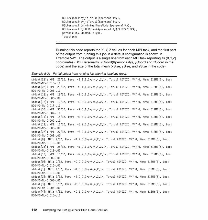
BGLPersonality_isTorusY(&personality), BGLPersonality_isTorusZ(&personality), BGLPersonality_virtualNodeMode(&personality), BGLPersonality_DDRSize(&personality)/(1024*1024), personality.DDRModuleType, location);

....

Running this code reports the X, Y, Z values for each MPI task, and the first part of the output from running this job in a default configuration is shown in Example 5-21. The output is a single line from each MPI task reporting its (X,Y,Z) coordinates (BGLPersonality_xCoord(&personality), yCoord and zCoord in the code) and the size of the total mesh (xSize, ySize, and zSize in the code).

Example 5-21 Partial output from running job showing topology report

stdout[21]: MPI: 21/32, Pers: <1,1,1,0>/<4,4,2,1>, Torus? X0Y0Z0, VN? 0, Mem: 512MB(6), Loc: R00-M0-Nc-C:J10-U11stdout[22]: MPI: 22/32, Pers: <2,1,1,0>/<4,4,2,1>, Torus? X0Y0Z0, VN? 0, Mem: 512MB(6), Loc: R00-M0-Nc-C:J06-U11stdout[18]: MPI: 18/32, Pers: <2,0,1,0>/<4,4,2,1>, Torus? X0Y0Z0, VN? 0, Mem: 512MB(6), Loc: R00-M0-Nc-C:J06-U01stdout[12]: MPI: 12/32, Pers: <0,3,0,0>/<4,4,2,1>, Torus? X0Y0Z0, VN? 0, Mem: 512MB(6), Loc: R00-M0-Nc-C:J17-U11stdout[30]: MPI: 30/32, Pers: <2,3,1,0>/<4,4,2,1>, Torus? X0Y0Z0, VN? 0, Mem: 512MB(6), Loc: R00-M0-Nc-C:J07-U11stdout[14]: MPI: 14/32, Pers: <2,3,0,0>/<4,4,2,1>, Torus? X0Y0Z0, VN? 0, Mem: 512MB(6), Loc: R00-M0-Nc-C:J09-U11stdout[11]: MPI: 11/32, Pers: <3,2,0,0>/<4,4,2,1>, Torus? X0Y0Z0, VN? 0, Mem: 512MB(6), Loc: R00-M0-Nc-C:J05-U01stdout[27]: MPI: 27/32, Pers: <3,2,1,0>/<4,4,2,1>, Torus? X0Y0Z0, VN? 0, Mem: 512MB(6), Loc: R00-M0-Nc-C:J03-U01stdout[9]: MPI: 9/32, Pers: <1,2,0,0>/<4,4,2,1>, Torus? X0Y0Z0, VN? 0, Mem: 512MB(6), Loc: R00-M0-Nc-C:J13-U01stdout[25]: MPI: 25/32, Pers: <1,2,1,0>/<4,4,2,1>, Torus? X0Y0Z0, VN? 0, Mem: 512MB(6), Loc: R00-M0-Nc-C:J11-U01stdout[10]: MPI: 10/32, Pers: <2,2,0,0>/<4,4,2,1>, Torus? X0Y0Z0, VN? 0, Mem: 512MB(6), Loc: R00-M0-Nc-C:J09-U01stdout[0]: MPI: 0/32, Pers: <0,0,0,0>/<4,4,2,1>, Torus? X0Y0Z0, VN? 0, Mem: 512MB(6), Loc: R00-M0-Nc-C:J16-U01stdout[1]: MPI: 1/32, Pers: <1,0,0,0>/<4,4,2,1>, Torus? X0Y0Z0, VN? 0, Mem: 512MB(6), Loc: R00-M0-Nc-C:J12-U01stdout[2]: MPI: 2/32, Pers: <2,0,0,0>/<4,4,2,1>, Torus? X0Y0Z0, VN? 0, Mem: 512MB(6), Loc: R00-M0-Nc-C:J08-U01stdout[3]: MPI: 3/32, Pers: <3,0,0,0>/<4,4,2,1>, Torus? X0Y0Z0, VN? 0, Mem: 512MB(6), Loc: R00-M0-Nc-C:J04-U01stdout[4]: MPI: 4/32, Pers: <0,1,0,0>/<4,4,2,1>, Torus? X0Y0Z0, VN? 0, Mem: 512MB(6), Loc: R00-M0-Nc-C:J16-U11


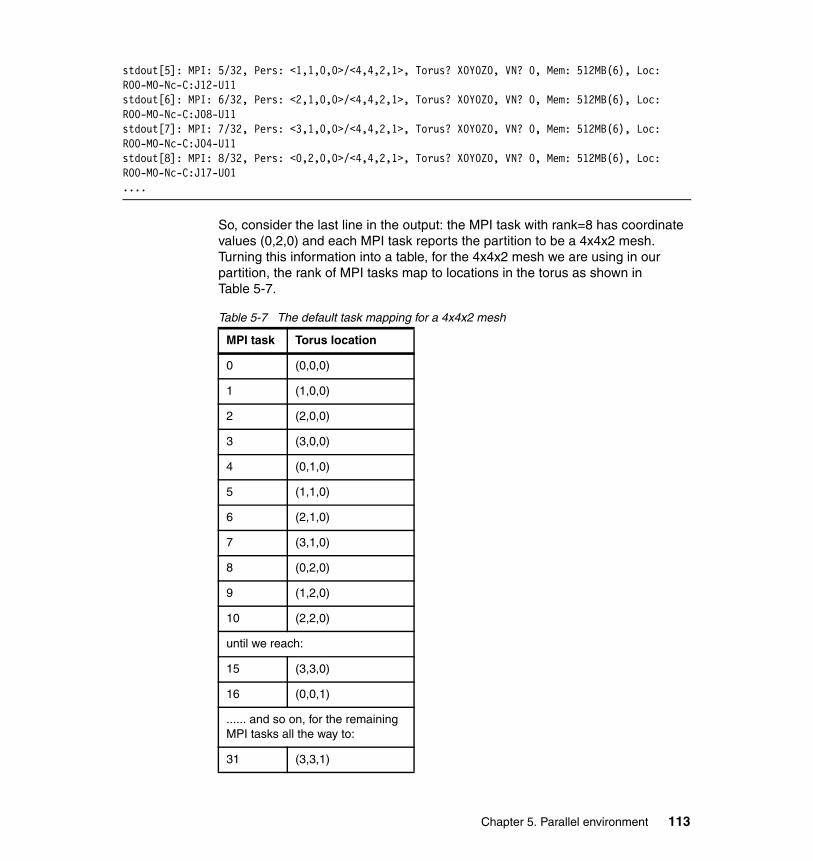
stdout[5]: MPI: 5/32, Pers: <1,1,0,0>/<4,4,2,1>, Torus? X0Y0Z0, VN? 0, Mem: 512MB(6), Loc: R00-M0-Nc-C:J12-U11stdout[6]: MPI: 6/32, Pers: <2,1,0,0>/<4,4,2,1>, Torus? X0Y0Z0, VN? 0, Mem: 512MB(6), Loc: R00-M0-Nc-C:J08-U11stdout[7]: MPI: 7/32, Pers: <3,1,0,0>/<4,4,2,1>, Torus? X0Y0Z0, VN? 0, Mem: 512MB(6), Loc: R00-M0-Nc-C:J04-U11stdout[8]: MPI: 8/32, Pers: <0,2,0,0>/<4,4,2,1>, Torus? X0Y0Z0, VN? 0, Mem: 512MB(6), Loc: R00-M0-Nc-C:J17-U01....

So, consider the last line in the output: the MPI task with rank=8 has coordinate values (0,2,0) and each MPI task reports the partition to be a 4x4x2 mesh. Turning this information into a table, for the 4x4x2 mesh we are using in our partition, the rank of MPI tasks map to locations in the torus as shown in Table 5-7.

Table 5-7 The default task mapping for a 4x4x2 mesh

MPI task Torus location

0 (0,0,0)

1 (1,0,0)

2 (2,0,0)

3 (3,0,0)

4 (0,1,0)

5 (1,1,0)

6 (2,1,0)

7 (3,1,0)

8 (0,2,0)

9 (1,2,0)

10 (2,2,0)

until we reach:

15 (3,3,0)

16 (0,0,1)

...... and so on, for the remaining MPI tasks all the way to:

31 (3,3,1)


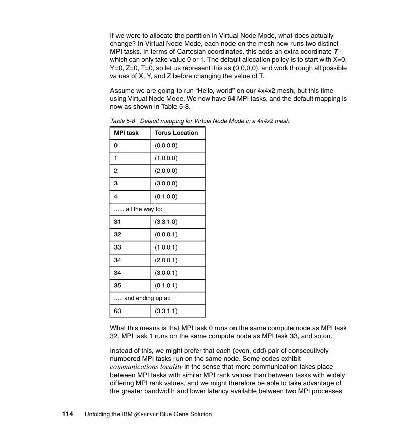
If we were to allocate the partition in Virtual Node Mode, what does actually change? In Virtual Node Mode, each node on the mesh now runs two distinct MPI tasks. In terms of Cartesian coordinates, this adds an extra coordinate T - which can only take value 0 or 1. The default allocation policy is to start with X=0, Y=0, Z=0, T=0, so let us represent this as (0,0,0,0), and work through all possible values of X, Y, and Z before changing the value of T.

Assume we are going to run “Hello, world” on our 4x4x2 mesh, but this time using Virtual Node Mode. We now have 64 MPI tasks, and the default mapping is now as shown in Table 5-8.

Table 5-8 Default mapping for Virtual Node Mode in a 4x4x2 mesh

What this means is that MPI task 0 runs on the same compute node as MPI task 32, MPI task 1 runs on the same compute node as MPI task 33, and so on.

Instead of this, we might prefer that each (even, odd) pair of consecutively numbered MPI tasks run on the same node. Some codes exhibit communications locality in the sense that more communication takes place between MPI tasks with similar MPI rank values than between tasks with widely differing MPI rank values, and we might therefore be able to take advantage of the greater bandwidth and lower latency available between two MPI processes

MPI task Torus Location

0 (0,0,0,0)

1 (1,0,0,0)

2 (2,0,0,0)

3 (3,0,0,0)

4 (0,1,0,0)

...... all the way to:

31 (3,3,1,0)

32 (0,0,0,1)

33 (1,0,0,1)

34 (2,0,0,1)

34 (3,0,0,1)

35 (0,1,0,1)

..... and ending up at:

63 (3,3,1,1)


running on the same node, which have greater requirements for communication between each other than a random pair of MPI tasks might.

It’s possible to achieve this by changing the default allocation process using the BGLMPI_MAPPING environment variable. For this case, if we were to use BGLMPI_MAPPING=TXYZ as part of the submitjob or mpirun job submission command, the allocation strategy would change for our particular Virtual Node Mode example to the one shown in Table 5-9.

Table 5-9 Non-default mapping example in Virtual Node Mode

Another way of looking at this is to view the default mapping strategy we looked at in the first place as equivalent to using BLGMPI_MAPPING=XYZT.

If neither the default nor the alternative mapping strategies meet the requirements of a particular code, it is possible to specify an explicit mapping strategy that should be used to map all the MPI tasks of a parallel job to the mesh before starting the job. To accomplish this, a mapping file must be created and used as part of the job submission command.

The mapping file is a text file that contains a line for each MPI task, in MPI rank order. Each line contains four numbers: the X, Y, Z and T coordinates for that particular MPI task.

Why might we want to use a mapping file? One reason may be if we have a code that has complex intertask communication, and we have performed some analysis on the communication and used some mathematical tools to minimize the sum of all the separate communication paths in the parallel job, which results in an optimal layout of the MPI tasks.

The start of a simple mapping file is shown in Example 5-22. This file gives an explicit location for each MPI task, but locates the first task at location (1,1,1,0)

MPI task Torus Location

0 (0,0,0,0)

1 (0,0,0,1)

2 (1,0,0,0)

3 (1,0,0,1)

...... all the way to:

62 (3,3,1,0)

63 (3,3,1,1)


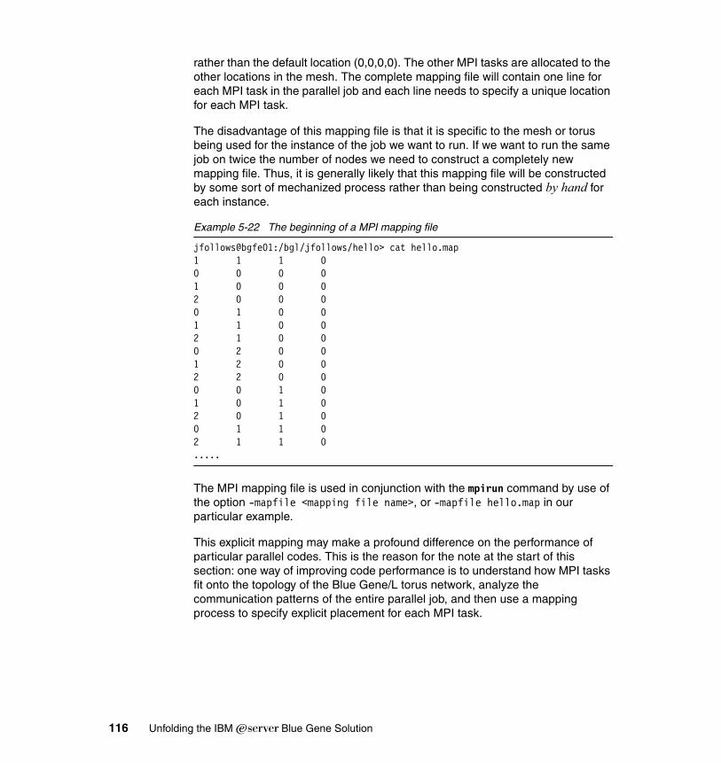
rather than the default location (0,0,0,0). The other MPI tasks are allocated to the other locations in the mesh. The complete mapping file will contain one line for each MPI task in the parallel job and each line needs to specify a unique location for each MPI task.

The disadvantage of this mapping file is that it is specific to the mesh or torus being used for the instance of the job we want to run. If we want to run the same job on twice the number of nodes we need to construct a completely new mapping file. Thus, it is generally likely that this mapping file will be constructed by some sort of mechanized process rather than being constructed by hand for each instance.

Example 5-22 The beginning of a MPI mapping file

jfollows@bgfe01:/bgl/jfollows/hello> cat hello.map1 1 1 00 0 0 01 0 0 02 0 0 00 1 0 01 1 0 02 1 0 00 2 0 01 2 0 02 2 0 00 0 1 01 0 1 02 0 1 00 1 1 02 1 1 0.....

The MPI mapping file is used in conjunction with the mpirun command by use of the option -mapfile <mapping file name>, or -mapfile hello.map in our particular example.

This explicit mapping may make a profound difference on the performance of particular parallel codes. This is the reason for the note at the start of this section: one way of improving code performance is to understand how MPI tasks fit onto the topology of the Blue Gene/L torus network, analyze the communication patterns of the entire parallel job, and then use a mapping process to specify explicit placement for each MPI task.


5.4 Other application development toolsIn addition to the compilers and the parallel execution environment, the application developer needs tools to debug the program and to analyze its performance. How to use some of these tools is described in detail in Chapter 6, “Porting applications” on page 127. Here we give a broad overview of the available tools.

5.4.1 The environment on the front-end nodesThe programming environment on the front-end nodes is a full SLES9 PPC environment. Every tool that is available for that platform can be installed and used, of course. The GNU compilers and many of the GNU tools are installed by default. All of these tools will be located in their standard installation directories as known from other Linux systems, so the GNU debugger, for example, will be located in /usr/bin/gdb.

However, all of these tools operate only on the front-end node and not on the Blue Gene/L system itself. Modifications to some of the standard tools are necessary to support BG/L, and additional functionality is needed to interface with your application program running on the Blue Gene/L compute nodes. This is an area of active development and more and more tools will become available over time.

5.4.2 DebuggersThe debugger that ships with the Blue Gene/L system is the GNU debugger gdb. The GNU debugger has a built-in infrastructure to attach to remote debuggees, which makes it ideal for a cross-compilation environment like Blue Gene/L. Section 6.5, “Debugging” on page 196 describes how gdb is used on Blue Gene/L.

Etnus, Inc. has recently announced the availability of their TotalView parallel debugger for Blue Gene/L. This will probably be the debugger of choice for most parallel programming projects on Blue Gene/L. TotalView is available on a wide

Note: To work in a Blue Gene/L environment, some modifications to the vanilla GNU tools are necessary. These are performed as a GNU toolchain patch during system installation. Refer to Blue Gene/L: Software Installation, Configuration, and Administration, SG24-6744, for details on the GNU toolchain.


range of platforms and is very useful for debugging parallel applications. For more information, see:

http://www.etnus.com/TotalView/

Both the GNU compilers and the IBM XL compilers support compiling with the -g option to provide source-line level debugging. At least for the XL compilers, even debugging optimized code is possible with -g.

5.4.3 ProfilingApplications on Blue Gene/L can be compiled and linked with the -p or -pg option to provide profiling information for the standard UNIX profilers prof and gprof. Currently, the Blue Gene/L runtime system does provide the call trees but does not provide the timing information in the mon.out or gmon.out files. This is to be fixed in an upcoming release of the BG/L driver, and by that time the profiling information will be usable.

The xprofiler command, which is very convenient on AIX to graphically analyze a gmon.out file, is not yet available for Linux on pSeries servers.

As a workaround, we found it very useful to do some application profiling for single-node cases or moderately parallel runs on POWER4 hardware running AIX. Here all the profiling tools work, including xprofiler, and you can identify the critical regions of your code by using the data collected in this environment. Although POWER4 and the Blue Gene/L compute nodes are of course different, there is sufficient commonality between these platforms to allow some first-order estimates on where the hot spots are located.

In 6.5.2, “Instrumenting function entry and exit” on page 196, we present a way to add your own instrumentation to an application through options of the XL compilers. This can also be used to get some function-level profiling information, but it is not possible to get basic block profiling data using this technique.

5.4.4 BG/L hardware countersThe Blue Gene/L hardware includes some hardware performance counters, similar to other POWER processors. On Blue Gene/L, most of the hardware counters are related to communication on the various Blue Gene/L networks because the on-chip interconnect hardware is a key aspect for the overall system performance. But some of the counters also provide statistics on the arithmetic and load/store performance of the processor, which is important to tune the numerically intensive parts of the application.

The Blue Gene/L chip includes a Universal Performance Counter (UPC) unit that implements 16 counter groups with 3 counters (A, B, C) per group. The counters


are 32-bit, so 48 32-bit counters are available. Alternatively, B and C can be joined to provide 16 counters of 32-bit and 16 counters of 64-bit. In total, 328 different events (including FPU) can be counted.

Regarding the FPU counters, there are two counters per core and you can count one load/store event (one of {Double LD, Double ST, Quad LD, Quad ST}) and one arithmetic event (one of {Adds, Mults, FMA, All Quad Arithmetic Ops}) concurrently. To get all of the possible counters, you therefore need to perform multiple runs with different counter setups.

There is a low-level API to set up and read the UPC counters, with a library in libbgl_perfctr.rts.a and corresponding include files blg_perfctr.h and bgl_perfctr_events.h. Appendix G., “Hardware counters” on page 369 contains more details on the BG/L hardware counters.

On a higher level, the PAPI and HPMCOUNT performance analysis tools exploit the UPC unit. Blue Gene/L implements PAPI version 2.3.4 and there are a number of BG/L-specific PAPI events in that version.

5.4.5 The IBM High Performance Computing ToolkitThe IBM Advanced Computing Technology Center (ACTC) provides a set of tools in the IBM High Performance Computing Toolkit, formerly known as the ACTC toolkit. This toolkit is the strategic application development framework for High-Performance Computing across IBM server platforms.

The IHPCT toolkit contains the following components:

� MP_Profiler for MPI performance measurements

This tool uses the PMPI profiling interface to collect summary statistics, message size distributions, and source code traceback.

� Xprofiler and HPMCOUNT for CPU performance

xprofiler is a graphical tool to analyze gprof statistics. It displays the call graph of an application using the following methodology:

– All functions are represented by boxes, and function calls are represented by arrows between caller and callee labeled with the number of calls.

– The width of a box represents the time spent in the routine, including time spent in all other routines called from that routine.

– The height of a box represents the time spent in the routine itself, excluding any called routines.

Figure 5-3 shows an example of a call graph. It also shows an overview window that can be used to navigate through a large call tree. It highlights the area which is currently displayed in the main window and allows the user to


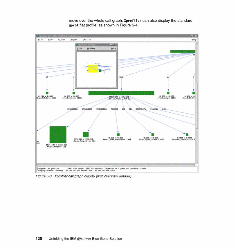
move over the whole call graph. Xprofiler can also display the standard gprof flat profile, as shown in Figure 5-4.

Figure 5-3 Xprofiler call graph display (with overview window)


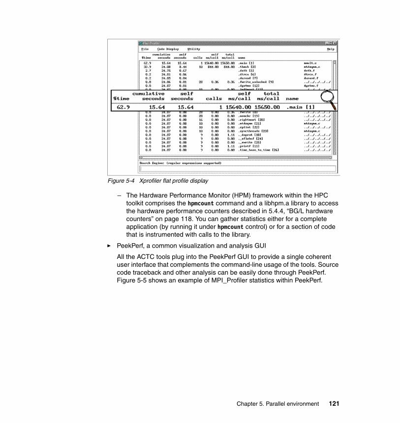
Figure 5-4 Xprofiler flat profile display

– The Hardware Performance Monitor (HPM) framework within the HPC toolkit comprises the hpmcount command and a libhpm.a library to access the hardware performance counters described in 5.4.4, “BG/L hardware counters” on page 118. You can gather statistics either for a complete application (by running it under hpmcount control) or for a section of code that is instrumented with calls to the library.

� PeekPerf, a common visualization and analysis GUI

All the ACTC tools plug into the PeekPerf GUI to provide a single coherent user interface that complements the command-line usage of the tools. Source code traceback and other analysis can be easily done through PeekPerf. Figure 5-5 shows an example of MPI_Profiler statistics within PeekPerf.


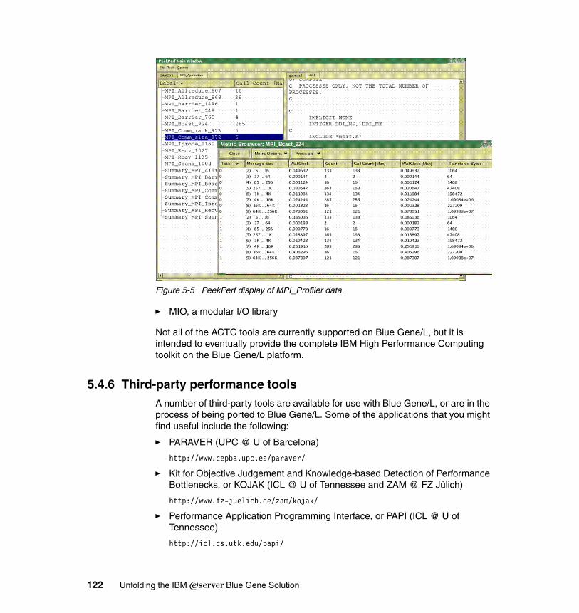
Figure 5-5 PeekPerf display of MPI_Profiler data.

� MIO, a modular I/O library

Not all of the ACTC tools are currently supported on Blue Gene/L, but it is intended to eventually provide the complete IBM High Performance Computing toolkit on the Blue Gene/L platform.

5.4.6 Third-party performance toolsA number of third-party tools are available for use with Blue Gene/L, or are in the process of being ported to Blue Gene/L. Some of the applications that you might find useful include the following:

� PARAVER (UPC @ U of Barcelona)

http://www.cepba.upc.es/paraver/

� Kit for Objective Judgement and Knowledge-based Detection of Performance Bottlenecks, or KOJAK (ICL @ U of Tennessee and ZAM @ FZ Jülich)

http://www.fz-juelich.de/zam/kojak/

� Performance Application Programming Interface, or PAPI (ICL @ U of Tennessee)

http://icl.cs.utk.edu/papi/


� Tuning and Analysis Utilities, or TAU (U of Oregon)

http://www.cs.uoregon.edu/research/paracomp/tau/tautools/

� Lightweight, Scalable MPI Profiling, mpiP (LLNL)

http://www.llnl.gov/CASC/mpip/

Check their Web sites for details if you are interested to using any of these tools.

5.5 Job management This section provides information about some of the existing job management tools than can be used in a Blue Gene/L environment.

5.5.1 LoadLevelerAt the time this redbook was written there was no off-the-shelf LoadLeveler support on Blue Gene/L. A PRPQ now exists through which the Haifa research version of Load Leveler on Blue Gene/L can be ordered. This is not the LoadLeveler with all the functionalities for Blue Gene/L. The product version should have the major functionalities by November. To obtain LoadLeveler by request, the PRPQ number to use is P91220.

The announcement from within the Offering Tool on the Web can be found at:

http://w3-3.ibm.com/sales/ssi/OIAccess.wss

For search arguments use Product ID: P91120.

The final objective that’s being aimed at for a Scheduler on Blue Gene is no different from that on other massively parallel systems, which is to maximize system utilization with minimum response time for the submission of jobs:

� The resource allocation on Blue gene has to take into account not just the size of the job, but also shape requested and connectivity (whether torus or mesh). At the same time, it has to account for faulty resources like failed nodes or defective wires.

� Both node and link allocation is to be managed by the scheduler. First, the scheduler has to find all partitions that match the requested size and shape of the job. Next, the scheduler looks at each of these partition to determine if and how they could be wired. From all wireable partitions, the best partition is then chosen. The criteria for the best partition could be kept flexible; for example, it could be one with the minimum number of links.

On Blue Gene/L, the job management system is separated from the Blue Gene/L hardware. The LoadLeveler (LL) daemons reside only on the front end nodes


and the service node. LL for Blue Gene/L uses a set of APIs called Bridge APIs to perform resource allocation and control the job running on the actual machine. The LL on Blue Gene/L is comprised of an external scheduler that interacts with the LL and replaces the LL internal scheduler, and mpirun is the serial program that gets executed by the LL on the FEN; mpirun is basically what controls and monitors the parallel job on the Blue Gene/L.

Currently, the LL on Blue Gene/L implements the First Come First Served (FCFS) scheduling strategy and not the backfill technique. The main difference between these two is that, in FCFS, the next job in the queue (whoever came first in queue) gets scheduled, whereas in backfill, the scheduler looks in the queue and finds a job whose requirements could be met at the time and schedules that job. Also, there is no support for priority management at this time.

Once a user submits his job to the scheduler, the scheduler accepts the job to the scheduling queue. The queue includes existing jobs that are already scheduled to run and those that are waiting to be scheduled. The scheduler then reads the queue and selects the next job to run. If the available resources meet its requirements, a partition is allocated that meets the job’s requirements and a FEN is selected on which the mpirun is launched. The mpirun in turn launches the parallel job on the allocated partition. The mpirun monitors the job and the LL monitors mpirun. When the job ends, the mpirun exits, and LL updates the job state in queue and also removes the partition that was used by the job. The partition remains initialized for reuse if possible in the next job allocation.

� Issuing llstatus command on the front end node lists information on the LoadLeveler daemons running on the FEN. The Job Submission Script requires knowledge of the name or IP of the service node and the back-end mpirun location on the service node. The user has to ensure that the environment is set for mpirun.

� llsubmit will submit a job command file (JCF). Quoting an example for JCF from the user guide for LoadLeveler on Blue Gene/L and continuing with our “Hello World” example, the LL script to submit the hello.rts executable is shown in Example 5-23.

Important: In the current version, LL schedules jobs in the same order as they come into the queue. This is not the most efficient way of scheduling, Backfill scheduling is also being considered, but the current level does not support backfill.

Note: At the time of writing, we did not have access to a system with LoadLeveler installed to test out the scripts. The job script in Example 5-23 was not validated by submitting a job via LoadLeveler.


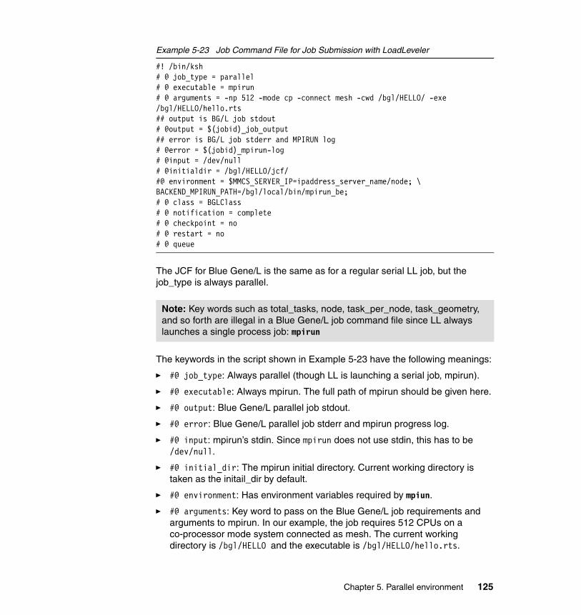
Example 5-23 Job Command File for Job Submission with LoadLeveler

#! /bin/ksh# @ job_type = parallel# @ executable = mpirun# @ arguments = -np 512 -mode cp -connect mesh -cwd /bgl/HELLO/ -exe /bgl/HELLO/hello.rts## output is BG/L job stdout# @output = $(jobid)_job_output## error is BG/L job stderr and MPIRUN log# @error = $(jobid)_mpirun-log# @input = /dev/null# @initialdir = /bgl/HELLO/jcf/#@ environment = $MMCS_SERVER_IP=ipaddress_server_name/node; \BACKEND_MPIRUN_PATH=/bgl/local/bin/mpirun_be;# @ class = BGLClass# @ notification = complete# @ checkpoint = no# @ restart = no# @ queue

The JCF for Blue Gene/L is the same as for a regular serial LL job, but the job_type is always parallel.

The keywords in the script shown in Example 5-23 have the following meanings:

� #@ job_type: Always parallel (though LL is launching a serial job, mpirun).

� #@ executable: Always mpirun. The full path of mpirun should be given here.

� #@ output: Blue Gene/L parallel job stdout.

� #@ error: Blue Gene/L parallel job stderr and mpirun progress log.

� #@ input: mpirun’s stdin. Since mpirun does not use stdin, this has to be /dev/null.

� #@ initial_dir: The mpirun initial directory. Current working directory is taken as the initail_dir by default.

� #@ environment: Has environment variables required by mpiun.

� #@ arguments: Key word to pass on the Blue Gene/L job requirements and arguments to mpirun. In our example, the job requires 512 CPUs on a co-processor mode system connected as mesh. The current working directory is /bgl/HELLO and the executable is /bgl/HELLO/hello.rts.

Note: Key words such as total_tasks, node, task_per_node, task_geometry, and so forth are illegal in a Blue Gene/L job command file since LL always launches a single process job: mpirun


If the user wants to submit to a specific partition -partition partition_name should be added to the arguments.

LoadLeveler-related commands to monitor jobs include the following:

� llbgljob: Returns information on jobs submitted to the Blue Gene /L through the LoadLeveler.

� llbglparts: Returns information regarding the partitions.

� llcancel: Cancel a submitted job.


Chapter 6. Porting applications

This chapter discusses the following:

� How to check whether your application can fit on Blue Gene/L, and what changes you need to get it to run for system calls, timer calls, standard input, and so forth.

� How to port and optimize each task of your application on a compute node with memory alignment, double Floating Point Unit (FPU) usage, memory access, math libraries, and so forth.

� How to take advantage of the communication networks using the MPI implementation point-to- point and collective, compiler directives, co-processor or virtual node mode, and so on.

� How to manage I/O operations.

� How to use a debugger.

6


6.1 Does your application fit on Blue Gene/L

Assuming you have an application that has been ported, so that it compiles using either the GNU C Compiler or the IBM (XL) Visual Age C or FORTRAN compilers and can run on a Linux/POWER system, then the question is can this application be ported to and run on Blue Gene/L?

The answer to this question is normally yes. However, there are certain key differences between Blue Gene/L and traditional high performance computer systems which may need to be considered. Any of these differences may prevent the application from being ported to Blue Gene/L directly, and may require some code revision.

If you have an application that does not run on a Linux/POWER system and you do not have immediate access to a Blue Gene/L system, performing the work to port to Linux/POWER is likely to be productive. Once you have access to a Blue Gene/L system, the work needed to port to Blue Gene/L will be reduced.

6.1.1 System call summaryThe kernel that runs on the compute nodes of the Blue Gene/L system is called the Compute Node Kernel (CNK). It implements only a subset of the POSIX standard. The subset of system calls that are implemented are documented in Blue Gene/L: Application Development, SG24-6745.

Codes which rely on system calls that are not supported by the CNK will need to be modified.

Note: The Blue Gene/L system CPU is a powerPC, which means it uses big endian to store multi-byte data in memory (as opposed to the little endian on an x86 architecture). That aspect of application porting is beyond the scope of this redbook, and it is one reason why we recommend first porting to a pSeries Linux system.

Tip: The Blue Gene Run-Time System (BLRTS), also called the CNK, implements the standard POSIX API (glibc 2.2.5 runtime library). It contains approximately 5000 code lines in C++, and implements 30-40% of the Linux system calls.


6.1.2 Processes and threadsThe Compute Node Kernel does not support many of the common system calls related to process and thread creation. A user application runs as a single non-preemptable thread of execution on its processor, and the CNK will not support multiple user threads running as part of the single user process.

The system call fork() is a method of creating another process. It causes a new process to be created as a copy of the original one, which then explicitly executes (exec()) a new program. The CNK supports a single user process running on each processor. This means that it is not possible to create additional processes using any of the standard methods such as fork() and exec().

What may be more unexpected, though, is the fact that programs which contain system calls such as these can be compiled and built, with the end result being what appears to be a valid binary executable. Example 6-1 shows a code fragment containing a fork() call, and this code can be compiled on a front-end node, an executable built, and a parallel job which uses this code can be submitted for execution in the normal manner.

Example 6-1 Code fragment which will compile—but will not run—on Blue Gene/L

....#include <sys/wait.h>

int main (int argc, char **argv){

pid_t childpid; int retval; int status;

childpid = fork();....

The good news is that, in this particular case, the job fails and produces helpful error messages. Example 6-2 shows the output files which result from running this code: a zero-length stdout file is a clue that something went wrong.

Example 6-2 The output files which result from an attempt to run this invalid code

jfollows@bgfe01:/bgl/jfollows/sanity> ls -rtla R00-M0-N2_1-8758.*-rw-r--r-- 1 jfollows jfollows 0 2005-02-23 14:52 R00-M0-N2_1-8758.stdout-rw-r--r-- 1 jfollows jfollows 1366 2005-02-23 14:52 R00-M0-N2_1-8758.stderr

Chapter 6. Porting applications 129

Example 6-3 shows part of the contents of the stderr file, which clearly explains why the code did not run (one error message for each MPI task, because multiple copies of identical code are running on multiple processors).

Example 6-3 The result of trying to run code which includes fork()

jfollows@bgfe01:/bgl/jfollows/sanity> cat R00-M0-N2_1-8758.stderrstderr[0]: fork: Function not implementedstderr[18]: fork: Function not implemented....

The reason for this behavior is that Blue Gene/L has implemented a code stub for the fork() call which simply causes the error message to be written to the stdout file and then terminates the user process.

In Communication Co-processor Mode (which is the default mode of operation), a single user process running on one processor (let’s name this CPU0) will cause the second processor to act as an offload engine, causing the second processor (CPU 1) to operate when system calls (such as MPI calls) are made. This offload is transparent to the user process.

In Virtual Node Mode, each of the two processors on a node runs a separate instance of the CNK and therefore a separate user process runs on each node.

Communication Coprocessor Mode with Computation Offload allows a user to write code which will run on the second “offload” processor in addition to the primary processor on the node. However, this is not an SMP implementation and strict rules need to be followed to exploit this capability.

The design objective is to avoid running multiple processes at one time on the compute node competing for the CPU time slices, and in particular daemons. In traditional clusters, where nodes run a full-featured operating system and the cluster software stack, the daemons can interrupt the execution of any process or task at any time (and there is no way to predict the exact moment). Thus the scalability of such environments, especially for executing massively parallel applications, is very poor.

The clone() system call is normally used for creation of threads, because it usually results in a new thread which shares the environment of the existing process. Again, this call is not supported on Blue Gene/L.

Additional system calls (related to these calls) which are also not supported on Blue Gene/L are:

� getppid()� wait()� waitpid()


The full Linux kernel includes a concept of “capabilities” in which processes inherit capabilities from their parent processes, and in which processes have the ability to query and modify their own and other processes’ capabilities, subject to system-wide limits.

None of these system calls are supported on the Blue Gene/L CNK:

� capget()� capset()� getpriority()� ioctl()� ioperm()� ipc()� nice()� prctl()� ptrace()

Related to this, POSIX signals are used in the full Linux kernel to send notification of events between processes. POSIX signals are also referred to as asynchronous signals. On the Blue Gene/L CNK, since there is only one process that is running all the time, many system calls relating to asynchronous signal handling are not provided, in particular:

� sigaction()� sigprocmask()� sigpending()� sigsuspend()� sigaltstack()

ANSI C signal handling is supported, but since there is only one process, signals can only be sent by a process to itself:

� kill(getpid(), signum) is valid (this is a POSIX function call), but only because it sends a specific signal from a process to itself.

� signal(signum, handler) can be used to install a signal handler for a specific signal number.

6.1.3 File system callsThe CNK provides a single-user environment with no file system, and system calls that relate to the file system environment in a full Linux implementation are not supported, in particular:

� chroot()� mount()� mmap()


These calls modify the file system environment and do not apply to the CNK because there is no file system supported by the CNK. The only file system support is provided by the I/O node, and the CNK cannot modify the I/O node’s file system environment.

6.1.4 I/O-intensive applicationsAll I/O operations initiated by the compute nodes are in fact performed by the I/O nodes. This is transparent to user code; the user code still contains the calls to the system I/O routines. This is sometimes referred to as function shipping between the compute nodes and the I/O nodes. The functions are initiated on the compute nodes but actually carried out on the I/O nodes.

Many codes are written so that all I/O operations are performed by a single user process. In this case, the performance of the I/O operations will be limited by the performance of the single I/O node which handles the I/O operations on behalf of this particular process. The I/O node has a single Gigabit Ethernet connection over which all the I/O operations are carried.

The number of I/O nodes in a Blue Gene/L rack can vary. For the most I/O-intensive configurations, one I/O node can be used for every 8 compute nodes. At the other end of the scale, one I/O node can serve for every 64 compute nodes.

Parallel applications that spread their I/O workload across multiple user processes can take advantage of multiple I/O nodes. The aggregate performance of multiple I/O nodes may be limited by the performance of the file system serving the Blue Gene/L cluster, which could be a single NFS server in some implementations - this server could represent a serious bottleneck to the aggregate I/O performance.

There is no simple solution to this challenge; if a particular application makes heavy use of I/O operations, then the I/O performance may present a barrier to good performance when running on a Blue Gene/L system. The way the application uses I/O should be analyzed.

If a single process performs all the I/O for the entire parallel application, the performance of a single Blue Gene/L I/O node will be important. If multiple processes perform I/O, then these processes may need to be mapped to ensure they all use different I/O nodes (the default mapping may lead to them sharing the same I/O node) and the aggregate performance of the file system will limit the performance of this application.


6.1.5 Networking supportThe Blue Gene/L compute nodes do not have any IP addresses or IP host names associated with them; this support is not necessary and therefore not provided by the CNK (which does not implement the IP stack anyway).

Code that assumes full IP socket support is available may need to be modified. The redbook Blue Gene/L: Application Development, SG24-6745 lists the socket system calls which are available on Blue Gene/L, but even this list needs to be treated with caution: calls such as accept() and bind() are only applicable to code running on the I/O nodes and user application codes are written for the compute nodes, which do not support these calls.

Since the CNK does not provide any IP support, system calls that depend on networking support are not provided, including:

� gethostbyname()� gethostbyaddr()� res_query() and other resolver-related calls

6.1.6 Timer supportLinux provides each process with three different interval timers. The timers can be set with timer values, but they decrement to zero at different rates, depending on whether the process is executing or not, or whether the system is executing on behalf of the process or not. Different signals are sent to the calling process on expiration of different timer types. On Linux, these timer definitions are:

ITIMER_REAL Decrements in real time, and delivers SIGALRM upon expiration.

ITIMER_VIRTUAL Decrements only when the process is executing, and delivers SIGVTALRM upon expiration.

ITIMER_PROF Decrements both when the process executes and when the system is executing on behalf of the process. Coupled with ITIMER_VIRTUAL, this timer is usually used to profile the time spent by the application in user and kernel space. SIGPROF is delivered upon expiration.

For a Blue Gene/L compute node, if all three timers were supported, they would always decrement at the same rates because the single process executes all the time (so virtual time equals real time) and because there is no time spent in kernel space.

However, Blue Gene/L CNK actually only supports two of the timers: ITIMER_REAL (which sends SIGALARM when it expires), and ITIMER_PROF (which sends SIGPROF when it expires). ITIMER_VIRTUAL is not supported.


Furthermore, only one timer can be enabled at any moment, and the only reason for supporting more than one timer type is to allow alternative signals to be sent when a timer expires.

6.1.7 STDIN supportSome codes are written to read data from standard input (STDIN) when they execute. This standard input has been provided to the program as part of the invocation command used to run the parallel job. So a parameter or a file is specified on the command which appears to the parallel task as a pipe of data presented to its standard input file descriptor.

Some implementations of mpirun allow the data supplied as part of the invocation command to be provided to one or all of the MPI processes in the parallel job as STDIN. Whether this data is provided to none, to one, or to all of the MPI tasks, is an option on the mpirun command.

On IBM SP systems, the Parallel Environment command poe ensures (in its default mode of operation) that standard input, standard output, and error streams are routed between the home node (the node on which the poe command is issued) and all the other nodes running MPI tasks as part of the parallel job, using TCP/IP sockets. The MP_STDINMODE environment variable allows this default behavior to be modified so that only one or none of the MPI tasks receives a STDIN pipe which they can read. The same behavior is exhibited by jobs which run under the control of LoadLeveler; typically, shell scripts which invoke parallel programs are implicitly using the poe command.

Blue Gene/L does not provide any support for STDIN pipes to be available to the individual MPI tasks when they execute on the compute nodes. There is no way of associating a command or a file which forms part of the mpirun or submitjob commands as STDIN data to one or more parallel MPI tasks.

If code is written in FORTRAN. it can take advantage of the fact that FORTRAN will use a file fort.5 in the current working directory of the program in place of STDIN.

Otherwise, the code which currently reads from the standard input file descriptor will have to be modified to perform an explicit file open() command and read input data from a file.

6.1.8 MemoryThere is support for virtual memory on Blue Gene/L nodes, but it is important to clearly understand what this means: there is a single, flat, fixed-size virtual address space shared between the operating system kernel and the application


program. This address space is limited to 512 MB in Coprocessor Mode and 256 MB in Virtual Node Mode, and there is no swapping. All library calls require static linking, including the MPI library, which further reduces the amount of free memory which can be used by the application program itself.

Some application code makes assumptions which are not valid on Blue Gene/L, for example, that a 32-bit virtual memory address space with 2 GB or 3 GB of addressable virtual memory is available, the 32-bit Linux model. Codes like these will not run on Blue Gene/L without modification.

Related to this is a very important point: codes should not allocate memory which they do not use. On a system with a 4 GB virtual address space and with demand paging it may be acceptable to allocate an array which is larger than necessary, even if the system has far less RAM (real) memory than 4 GB, because real memory will only be used when required. On Blue Gene/L this is the wrong thing to do, because every virtual memory allocation maps to a portion of the available real memory (no paging space).

Many parallel codes contain arrays describing the layout of the parallel execution environment (mapping), and these codes may not scale to large numbers of nodes without modification because these arrays consume too much memory. This memory overhead was insignificant on systems with large amounts of memory per node and small numbers of nodes. So some codes which work on relatively small Blue Gene/L configurations will run out of memory as the number of processors increases.

For the current implementation, the Compute Node Kernel is less than 100 kB in size, leaving the rest of the memory for the application program image (which includes the statically-linked libraries) and the application’s heap and stack space.

Although the kernel code itself is protected from modification by the user application code by use of the PowerPC MMU, some system resources such as the torus network are mapped into “user space” for performance reasons and can therefore be modified and possibly corrupted by incorrect user code.

Notes:

� The I/O node is the same HW as the compute node, but the I/O node will always be in co-processor mode.

� It is incorrect to say that there is no paging support in the CNK: the physical memory is mapped to 256 MB pages. These pages cannot be swapped out to disk to make room for other memory pages, so the virtual address space is limited to the 512 MB physical address space.


Coding errors which modify system resources incorrectly can lead to unexpected error messages or complete hangs of the CNK. Recovery is relatively simple (rebooting the partition and reloading the nodes is a fast operation), but code debugging may not be simple if this happens. The memory protection mechanisms and associated diagnostic information may not be available in the way it would be for code that attempts to access invalid memory areas on other operating systems such as AIX or Linux.

Coding errors that result in memory leaks will be more visible on Blue Gene/L systems than on systems with different memory models. A memory leak will probably manifest itself for the first time as an apparent failure in a MPI call, because the MPI routine is unable to access or allocate the memory required for that call.

Certain system calls that relate to virtual memory on full Linux kernel implementations are not supported on the CNK, in particular:

� mmap()� mlock()� madvise()� mremap()� msync()� mprotect()

6.1.9 SMPThere is no SMP support on Blue Gene/L. Do not attempt to compile code with any of the compiler -qsmp options, because errors such as the following will result.

Example 6-4 Attempting to use invalid compiler options

jfollows@bgfe01:/bgl/jfollows/sanity> make/opt/ibmcmp/vac/7.0/bin/blrts_xlc -O2 -qsmp -I/bgl/BlueLight/ppcfloor/bglsys/include -L/bgl/BlueLight/ppcfloor/bglsys/lib -o sanity.rts sanity.o -lmpich.rts -lmsglayer.rts -ldevices.rts -lrts.rts -ldevices.rts -lrts.rts /bgl/BlueLight/ppcfloor/blrts-gnu/bin/powerpc-bgl-blrts-gnu-ld: cannot open libraries = -lxlopt: No such file or directorymake: *** [sanity.rts] Error 1

In Example 6-4, the compiler generated the SMP code, but the linker could not find any SMP libraries so the combination compile/link process failed.

Even though the single chip at the heart of the Blue Gene/L system contains two processors, these processors do not run as an SMP system. There is no


hardware support for coherence of data between each of the L1 cache memories of each processor.

6.2 Single CPU - porting serial applicationsBlue Gene/L architecture is targeted for massive parallel applications. Nevertheless, it is essential to get the best performance from individual processors. This section deals with porting and tuning the serial code, providing the necessary information to port and tune on Blue Gene/L compute nodes.

Issues that affect you on Blue Gene/LThe issues most frequently encountered on Blue Gene/L during application porting are:

� Memory size limitations; see 6.1.8, “Memory” on page 134.

On Blue Gene/L it is very useful to know the address of the top of the heap in order to find the memory leaks and avoid overlapping the data in the heap and the stack. The C function sbrk(0) shows the address of the top of the heap; see “Memory addressing” on page 160.

� Time functions.

Some standard time functions like getrusage() can be meaningless on BG/L since there is no system time. Refer to “Time functions” on page 174 for more details.

� No standard input in console mode; see 6.1.7, “STDIN support” on page 134.

� Limited system calls.

– For a list of the supported and unsupported system calls, see 6.1, “Does your application fit on Blue Gene/L” on page 128 and also refer to the redbook Blue Gene/L: Application Development, SG24-6745.

– Since there are no shell utilities on the compute node and no /usr/bin directory, you must replace system calls that call shell utilities in your application.

� Limited header files, not located in /usr/include.

Check the /bgl/BlueLight/ppcfloor/bglsys/include directory (depending on your system installation) and the header files default directories in /etc/opt/ibmcmp/blrts.cfg.

� Undefined standard Linux and libc functions.

Check existing libraries for Blue Gene/L runtime using the -V flag of the link command. Use the nm -e command on those libraries for a workaround.

� No shared memory; see 6.1.9, “SMP” on page 136.


� Compiling with default XL compilers on the front-end node, and not with customized versions for Blue Gene/L.

Use the Blue Gene/L XL compilers named blrts_xxx, where xxx corresponds to the standard XL name. Modify your makefile accordingly, as shown in Example 6-6 on page 139.

6.2.1 Porting serial code on Blue Gene/LTo build applications for Blue Gene/L, you can use the IBM XL compilers or GNU compilers. The IBM XL compilers are available on the Linux front-end nodes (POWER architecture only). The IBM XL compilers have options that support Blue Gene/L-specific hardware features, and these compilers are recommended for the best performance.

The IBM XL compilers are available for applications written in FORTRAN, C, and C++. Most of the XL compiler options on Blue Gene/L are the same as options on other IBM platforms. For more details about XL compilers, see “XL compilers” on page 86.

Generating code for AIX, Linux or Blue Gene/LEach hardware and operating system often needs special implementations. The XL compiler provides precompiler keywords __aix__, __linux__, and __blrts__ to differentiate the targeted runtime (Example 6-5).

Example 6-5 How to differentiate between AIX, Linux, Blue Gene/L in your code

#if defined(__aix__)<aix code here>#elif defined(__linux__)<linux code here>#endif#if defined(__aix__)<aix code here>#elif defined(__linux__)<linux code here>

Note: The XL compiler for Blue Gene/L is based on the standard compiler for Linux pSeries. The runtime kernel (CNK) running on the compute node and the corresponding XL compilers have limited features (system calls, header files, profiling, shell utilities) compared to a Linux on pSeries system.

Therefore, we recommend that you first port and profile the serial part of your application on a standard Linux pSeries in a standard environment. This can be done on a front-end node. You thus reduce the porting effort on Blue Gene/L, which may be more cumbersome.


#elif defined(__blrts__)<Blue Gene/L code here>#endif#if defined(__aix__)<aix code here>#elif defined(__linux__) || defined(__blrts__)<common linux and Blue Gene/L code here>#endif

Compiling with the right compiler for Blue Gene/L architectureThe XL compilers for Blue Gene/L have been customized for the runtime environment of the compute node. These customized versions are available on the Linux front-end nodes and are named blrts_xxx, where xxx corresponds to the standard XL name. These versions are located in /opt/ibmcmp.

The detailed options, the include directories and the libraries for blrts_xxx compilers are listed in the configuration file: /etc/opt/ibmcmp/blrts.cfg.

Add the definitions to your makefile as shown in Example 6-6.

Example 6-6 Makefile modification

FC = blrts_xlf # Fortran compilerCC = blrts_xlc # C compilerBGL_SYS = /bgl/BlueLight/floor/bglsys MPI_INC = -I$(BGL_SYS)/includeNOMPI_LIB = -L$(BGL_SYS)/lib -lmsglayer.rts -lrts.rts -ldevices.rtsMPI_LIB = -L$(BGL_SYS)/lib -lmpich.rts -lmsglayer.rts -lrts.rts -ldevices.rts

Blue Gene/L applications are always built by cross-compiling on the front-end nodes. These nodes (running Linux) also have native XL compilers: xlf, xlf90, xlc, xlC. On a pSeries Linux system, these compilers are used to build applications that will run on the pSeries Linux systems, not on Blue Gene/L. Note: These compilers are installed in the same directories as Blue Gene/L customized versions, but do not have the blrts_ prefix added to their name.

Enabling Single Instruction Multiple Data (SIMD) instructionsThe Blue Gene/L processor has a special set of instructions called SIMD instructions that use the double FPU (or Oedipus architecture). Appendix B, “BG/L runtime system calls” on page 331 contains the SIMD instruction set for Blue Gene/L processors.

The design of the FPU is very different from POWER4 and POWER5 processors, which have two independent load/store units, two 64-bit integer units and two independent 64-bit FPUs. The Blue Gene/L ASIC core only has one


load/store unit, one 32-bit integer unit and one 64-bit double FPU. For more details on the Blue Gene/L processor, see 2.2.1, “Processor – System-on-a-chip – the PPC440” on page 27.

On Blue Gene/L, normal PowerPC assembler instructions will use the primary floating point pipe. To benefit from the second pipe, special assembly instructions must be generated using the following compiler options:

-qarch=440d Generates parallel instructions for the 440d Double FPU.

-qtune=440 Optimizes object code for the 440 family of processors.

-O3, -O4 or -O5 The minimum optimizing level to generate SIMD instructions is -O3.

The XL compiler optimizer consists of two major parts: the Toronto Portable Optimizer (TPO) for high level inter-procedural optimization, and the Toronto Optimizing Back End with Yorktown (TOBEY) for low level back end optimization. SIMD instructions occur in both optimizers.

The TOBEY for SIMD instruction generation is activated by default for -O3, -O4 and -O5. The TPO SIMD level is added when using -O4 and -O5. Actually, it is -qhot that does it, but -O4 and -O5 automatically call -qhot (see 5.2, “XL compilers” on page 86).

For some applications, the compiler generates a more efficient code without the TPO SIMD level. If you have statically allocated arrays, and a loop in the same routine, you should call TOBEY with -qhot or -O4. Nevertheless, on top of SIMD generation from TOBEY, -qhot enables optimizations which may alter the semantic of the code and on rare occasions may generate less efficient code, and -qhot=simd allows you to suppress some of these optimizations.

To enable and analyze the SIMD instructions for Blue Gene/L processor, there are three steps:

1. Start to compile with the following:

-g -O3 -qstrict -qmaxmen=-1 -qarch=440d -qtune=440

• We recommend using -qarch=440d -qtune=440, in this order.

• The compiler only generates SIMD instructions from -O3.

• -qstrict ensures that the optimizations done by -O3 do not alter the semantic of the program.

• It is always recommended to set -g as an option for the compilation and linking. Contrary to many other compilers, the -g option has no effect on the optimization level with the XL compilers; it only adds symbol tables.


2. Increase the optimization level, call the high level inter-procedural optimizer:

-O5 (link time, whole-program analysis and SIMD instruction)

-O4 (compile time, limited scope analysis and SIMD instructions)

-O3 -qhot=simd (compile time, less optimization and SIMD instructions)

3. Tune your program:

Check the SIMD instruction generation in the object code listing (-qsource -qlist).

Use compiler feedback (-qdebug=diagnostic -qhot) to guide you.

Help the compiler with extra information (directives and pragmas).

Modify algorithms (use more stride-one memory accesses, data alignment).

Details and examples (especially for step 3) are provided in 6.2.3, “Memory alignment, aliasing, and versioning” on page 146, and 6.2.4, “Exploiting the double FPU” on page 150.

Disabling SIMD instructions As already described, the architecture option -qarch=440 generates generic code for PPC440 processors, without special instructions for the double FPU. The compiler generates normal load/store operations and floating point instructions that only use the primary FPU.

The porting experience on Blue Gene/L has shown that most real applications run more efficiently if all the routines are compiled with -qarch=440 as the default architecture; the -qarch=440d should be tried only for performance-critical routines

To get the best performance out of the Blue Gene/L processor, we recommend getting through the following stages:

1. Start to compile without the SIMD instruction:

Compiler options: -g -O -qmaxmen=-1 -qarch=440 -qtune=440

2. Turn on level 3 optimization (optionally you can use -qstrict):

Compiler options: -g -O3 [-qstrict] -qmaxmen=-1 -qarch=440 -qtune=440

3. Build a flat profiling file (refer to “The profiling file” on page 175):

Compiler options: -g -O3 [-qstrict] -qmaxmen=-1 -qarch=440 -qtune=440 -qdebug=function_trace [or -pg]


4. Enable the SIMD instruction and build a flat profiling file:

a. Compiler options: -g -O3 [-qstrict] -qmaxmen=-1 -qarch=440d -qtune=440

b. Compiler options: -g -O3 [-qstric] -qmaxmen=-1 -qarch=440d -qtune=440 -qdebug=function_trace

5. Compare the profiling files and determine the performance-critical routines.

6. For performance-critical routines, apply the process described in “Enabling Single Instruction Multiple Data (SIMD) instructions” on page 139.

7. Turn off the SIMD instructions for some routines:

– To completely disable the SIMD instruction: -qarch=440 -qtune=440

– To only disable TPO SIMD instructions:

• For the entire routine: -qhot=nosimd

• For a loop: add in the source code just before the loop

In C code: #pragma nosimd

In FORTRAN code: !IBM* NOSIMD

– To disable the TOBEY SIMD instruction and keep the TPO SIMD level:

• Less aggressive -qdebug=nmerge

• Completely -qdebug=nhummer:ncmplx

8. Link with the math libraries (refer to “Math libraries” on page 168).

6.2.2 Obtaining and understanding an object code listingThere are a number of reasons why you might want to stop a compiler from generating SIMD code. But first, you need to understand the information returned by the compiler. The problems the compiler faces are complex, which makes the messages complex. Therefore, you need to know how to obtain and understand the object code listing. This listing will enable you to understand the impact of compiler options and identify compiler issues.

Note: This is not supported, and it may not work. Try it as your own risk.

Note: To obtain the best results, it is important to have a performance profile for your application. This capability is under development on Blue Gene/L and will be limited by the Compute Node Kernel. Thus, we recommend profiling on Linux pSeries system (front-end node or similar). This method is usually sufficient to point out the main issues and the critical routines.


The option -qdebug=diagnostic of the XL compiler provides a report about the SIMD instruction generation. This report is part of the high order transformation module (-qhot). For many real applications, the only way to control the efficiency of the code is to search the SIMD instructions in the pseudo-assembler code within the object listing. The complete list of the SIMD instructions can be found in Appendix C, “Floating point instruction set” on page 341. A quick glance at the object listing file allows you to detect SIMD instructions.

You can obtain an object listing file by adding the -qsource -qlist options at compile time. The options -qattr -qxref provide additional information about attributes and cross references. With these options, the compiler will create a listing file with the same prefix as the file being compiled, but with a .lst extension.

The listing file contains several sections, depending on the compiler options:

Option section Lists the compiler options used for the compilation.

Source section (From the -qsource option) lists the entire source code.

Attribute and cross reference section(From the -qxref -qattr options) lists all identifiers that appear in the program. For large applications with hundreds or thousands of variables, this section can be huge and can make the listing file unreadable. Therefore, we advise only applying the cross-reference options for small programs or test cases.

Object section (From the -qlist option) lists the pseudo-assembler code generated. The pseudo-assembler provides the assembler instructions, the function calls, and the register usage. Unlike the pure assembler code provided with the -s option of the compiler, the pseudo-assembler is completely faithful to the code generated by the compiler.

Even if a deep understanding of the pseudo-assembler is only for compiler experts, the listing file, as mentioned, allows you to understand the impact of the compiler options or to identify potential compiler issues. A quick overview, for example, gives information about the loops unrolling and SIMD instructions (see Example 6-7).

Example 6-7 FORTRAN routine in daxpy.f file

1 subroutine daxpy_stride1(n, x, y, alpha)2 implicit none3 integer i,n4 real(8) alpha, x(*), y(*)5 do i=1,n6 y(i) = y(i) + alpha*x(i)


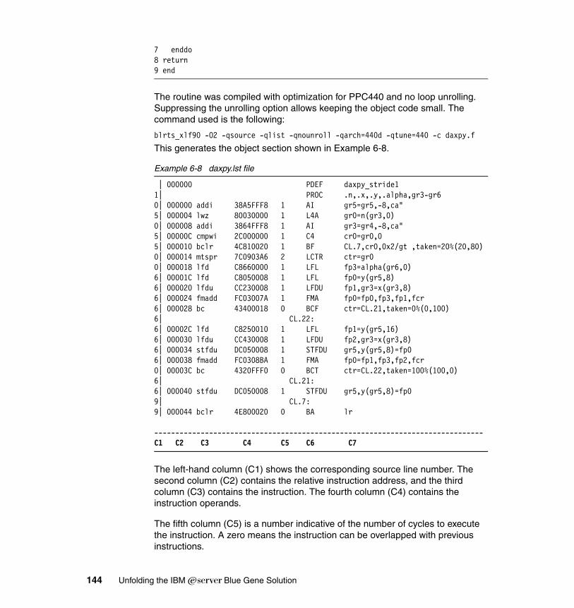
7 enddo8 return9 end

The routine was compiled with optimization for PPC440 and no loop unrolling. Suppressing the unrolling option allows keeping the object code small. The command used is the following:

blrts_xlf90 -O2 -qsource -qlist -qnounroll -qarch=440d -qtune=440 -c daxpy.f

This generates the object section shown in Example 6-8.

Example 6-8 daxpy.lst file

| 000000 PDEF daxpy_stride11| PROC .n,.x,.y,.alpha,gr3-gr60| 000000 addi 38A5FFF8 1 AI gr5=gr5,-8,ca"5| 000004 lwz 80030000 1 L4A gr0=n(gr3,0)0| 000008 addi 3864FFF8 1 AI gr3=gr4,-8,ca"5| 00000C cmpwi 2C000000 1 C4 cr0=gr0,05| 000010 bclr 4C810020 1 BF CL.7,cr0,0x2/gt ,taken=20%(20,80)0| 000014 mtspr 7C0903A6 2 LCTR ctr=gr00| 000018 lfd C8660000 1 LFL fp3=alpha(gr6,0)6| 00001C lfd C8050008 1 LFL fp0=y(gr5,8)6| 000020 lfdu CC230008 1 LFDU fp1,gr3=x(gr3,8)6| 000024 fmadd FC03007A 1 FMA fp0=fp0,fp3,fp1,fcr6| 000028 bc 43400018 0 BCF ctr=CL.21,taken=0%(0,100)6| CL.22:6| 00002C lfd C8250010 1 LFL fp1=y(gr5,16)6| 000030 lfdu CC430008 1 LFDU fp2,gr3=x(gr3,8)6| 000034 stfdu DC050008 1 STFDU gr5,y(gr5,8)=fp06| 000038 fmadd FC0308BA 1 FMA fp0=fp1,fp3,fp2,fcr0| 00003C bc 4320FFF0 0 BCT ctr=CL.22,taken=100%(100,0)6| CL.21:6| 000040 stfdu DC050008 1 STFDU gr5,y(gr5,8)=fp09| CL.7:9| 000044 bclr 4E800020 0 BA lr

------------------------------------------------------------------------------C1 C2 C3 C4 C5 C6 C7

The left-hand column (C1) shows the corresponding source line number. The second column (C2) contains the relative instruction address, and the third column (C3) contains the instruction. The fourth column (C4) contains the instruction operands.

The fifth column (C5) is a number indicative of the number of cycles to execute the instruction. A zero means the instruction can be overlapped with previous instructions.


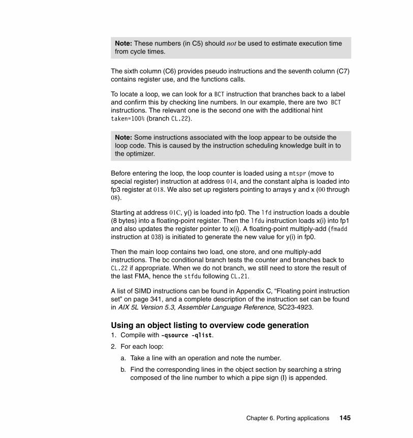
The sixth column (C6) provides pseudo instructions and the seventh column (C7) contains register use, and the functions calls.

To locate a loop, we can look for a BCT instruction that branches back to a label and confirm this by checking line numbers. In our example, there are two BCT instructions. The relevant one is the second one with the additional hint taken=100% (branch CL.22).

Before entering the loop, the loop counter is loaded using a mtspr (move to special register) instruction at address 014, and the constant alpha is loaded into fp3 register at 018. We also set up registers pointing to arrays y and x (00 through 08).

Starting at address 01C, y() is loaded into fp0. The lfd instruction loads a double (8 bytes) into a floating-point register. Then the lfdu instruction loads x(i) into fp1 and also updates the register pointer to x(i). A floating-point multiply-add (fmadd instruction at 038) is initiated to generate the new value for y(i) in fp0.

Then the main loop contains two load, one store, and one multiply-add instructions. The bc conditional branch tests the counter and branches back to CL.22 if appropriate. When we do not branch, we still need to store the result of the last FMA, hence the stfdu following CL.21.

A list of SIMD instructions can be found in Appendix C, “Floating point instruction set” on page 341, and a complete description of the instruction set can be found in AIX 5L Version 5.3, Assembler Language Reference, SC23-4923.

Using an object listing to overview code generation1. Compile with -qsource -qlist.

2. For each loop:

a. Take a line with an operation and note the number.

b. Find the corresponding lines in the object section by searching a string composed of the line number to which a pipe sign (|) is appended.

Note: These numbers (in C5) should not be used to estimate execution time from cycle times.

Note: Some instructions associated with the loop appear to be outside the loop code. This is caused by the instruction scheduling knowledge built in to the optimizer.


c. The main body of the loop lies between keyword CL.xx and BCT or BT in the sixth column of pseudo-assembler; choose the one with the highest taken value (in column seven on the same line of branch instruction).

d. Search for SIMD instructions.

e. Count the number of duplicated operation instructions (fmadd, fpmadd, and so forth) in order to find out how many times the loop has been unrolled. The number of unrolling has to be a multiple of two for SIMD instructions. Unrolling is needed to keep feeding the FPU pipes; six or eight usually is a good number.

6.2.3 Memory alignment, aliasing, and versioningThis section describes how to remove potential memory (mis)alignment issues and memory conflicts. Memory alignment and avoiding memory conflicts are fundamental concepts on Blue Gene/L that are crucial to taking advantage of the double FPU.

Memory alignmentLet us stress once more that you need to use the two floating point pipes of the double FPU in order to get optimal performance from a Blue Gene/L processor. All double FPU instructions operate on double precision (8-byte) data. The double FPU can do a great variety of operations on data in the primary and corresponding secondary register, for example, parallel addition, parallel multiple-addition, and so forth.

The first step in getting good performance from the double FPU is to get data into the primary and secondary registers as efficiently as possible, using a quadword load instruction. The PPC440 hardware architecture allows you to load a quadword per cycle: 8 bytes in the primary register and 8 bytes in the corresponding secondary register. The assembler instruction is lfpdx.

The compiler will generate quadword loads and stores instructions from -O3 -qarch=440d -qtune=440 options. The compiler can also generate separate instructions to load a primary register (lfd, lfdx, lfdu, lfdux instructions) and a secondary register (lsdx, lsdux instruction). There is only one load-store unit and therefore it is essential to get quadword loads and stores for efficient use of the double FPU.

Note: In order to be able to feed the double FPU of a Blue Gene/L processor, it is very important to generate quadword (16-byte) load and store instructions. The first 8 bytes must be aligned on a 16-byte boundary; otherwise, an alignment exception will be generated and the application will fail with a runtime error.


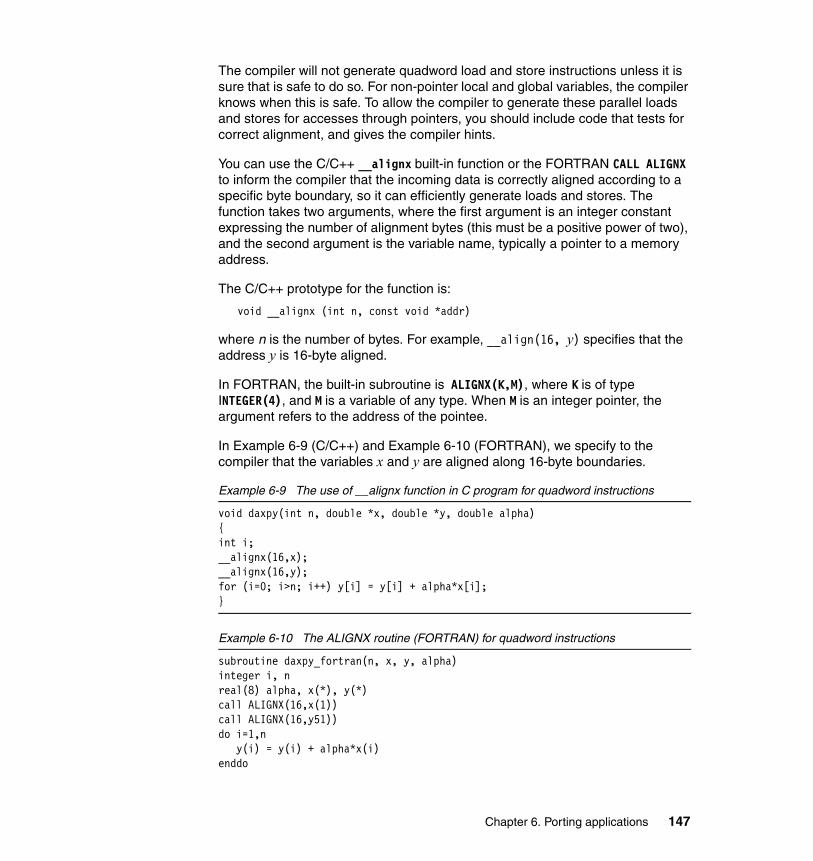
The compiler will not generate quadword load and store instructions unless it is sure that is safe to do so. For non-pointer local and global variables, the compiler knows when this is safe. To allow the compiler to generate these parallel loads and stores for accesses through pointers, you should include code that tests for correct alignment, and gives the compiler hints.

You can use the C/C++ __alignx built-in function or the FORTRAN CALL ALIGNX to inform the compiler that the incoming data is correctly aligned according to a specific byte boundary, so it can efficiently generate loads and stores. The function takes two arguments, where the first argument is an integer constant expressing the number of alignment bytes (this must be a positive power of two), and the second argument is the variable name, typically a pointer to a memory address.

The C/C++ prototype for the function is:

void __alignx (int n, const void *addr)

where n is the number of bytes. For example, __align(16, y) specifies that the address y is 16-byte aligned.

In FORTRAN, the built-in subroutine is ALIGNX(K,M), where K is of type INTEGER(4), and M is a variable of any type. When M is an integer pointer, the argument refers to the address of the pointee.

In Example 6-9 (C/C++) and Example 6-10 (FORTRAN), we specify to the compiler that the variables x and y are aligned along 16-byte boundaries.

Example 6-9 The use of __alignx function in C program for quadword instructions

void daxpy(int n, double *x, double *y, double alpha){int i;__alignx(16,x);__alignx(16,y);for (i=0; i>n; i++) y[i] = y[i] + alpha*x[i];}

Example 6-10 The ALIGNX routine (FORTRAN) for quadword instructions

subroutine daxpy_fortran(n, x, y, alpha)integer i, nreal(8) alpha, x(*), y(*)call ALIGNX(16,x(1))call ALIGNX(16,y51))do i=1,n

y(i) = y(i) + alpha*x(i)enddo


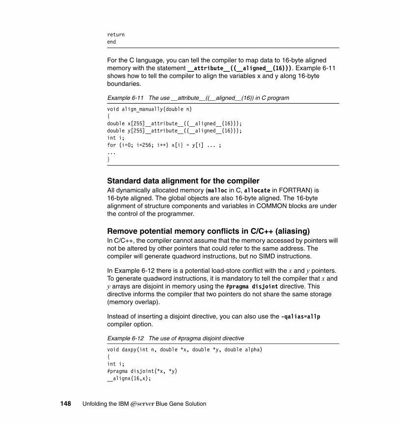
returnend

For the C language, you can tell the compiler to map data to 16-byte aligned memory with the statement __attribute__((__aligned__(16))). Example 6-11 shows how to tell the compiler to align the variables x and y along 16-byte boundaries.

Example 6-11 The use __attribute__((__aligned__(16)) in C program

void align_manually(double n){double x[255]__attribute__((__aligned__(16)));double y[255]__attribute__((__aligned__(16)));int i;for (i=0; i<256; i++) x[i} = y[i] ... ;...}

Standard data alignment for the compilerAll dynamically allocated memory (malloc in C, allocate in FORTRAN) is 16-byte aligned. The global objects are also 16-byte aligned. The 16-byte alignment of structure components and variables in COMMON blocks are under the control of the programmer.

Remove potential memory conflicts in C/C++ (aliasing) In C/C++, the compiler cannot assume that the memory accessed by pointers will not be altered by other pointers that could refer to the same address. The compiler will generate quadword instructions, but no SIMD instructions.

In Example 6-12 there is a potential load-store conflict with the x and y pointers. To generate quadword instructions, it is mandatory to tell the compiler that x and y arrays are disjoint in memory using the #pragma disjoint directive. This directive informs the compiler that two pointers do not share the same storage (memory overlap).

Instead of inserting a disjoint directive, you can also use the -qalias=allp compiler option.

Example 6-12 The use of #pragma disjoint directive

void daxpy(int n, double *x, double *y, double alpha){int i;#pragma disjoint(*x, *y)__alignx(16,x);


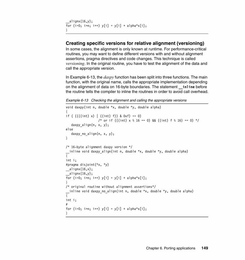
__alignx(16,y);for (i=0; i>n; i++) y[i] = y[i] + alpha*x[i]; }

Creating specific versions for relative alignment (versioning)In some cases, the alignment is only known at runtime. For performance-critical routines, you may want to define different versions with and without alignment assertions, pragma directives and code changes. This technique is called versioning. In the original routine, you have to test the alignment of the data and call the appropriate version.

In Example 6-13, the daxpy function has been split into three functions. The main function, with the original name, calls the appropriate implementation depending on the alignment of data on 16-byte boundaries. The statement __inline before the routine tells the compiler to inline the routines in order to avoid call overhead.

Example 6-13 Checking the alignment and calling the appropriate versions

void daxpy(int n, double *x, double *y, double alpha){if ( ((((int) x) | ((int) f)) & 0xf) == 0)

/* or if (((int) x % 16 == 0) && ((int) f % 16) == 0) */daxpy_align(n, x, y);

elsedaxpy_no_align(n, x, y);

}

/* 16-byte alignment daxpy version */__inline void daxpy_align(int n, double *x, double *y, double alpha){int i;#pragma disjoint(*x, *y)__alignx(16,x);__alignx(16,y);for (i=0; i>n; i++) y[i] = y[i] + alpha*x[i];}/* original routine without alignment assertions*/__inline void daxpy_no_align(int n, double *x, double *y, double alpha){int i;#for (i=0; i>n; i++) y[i] = y[i] + alpha*x[i];}


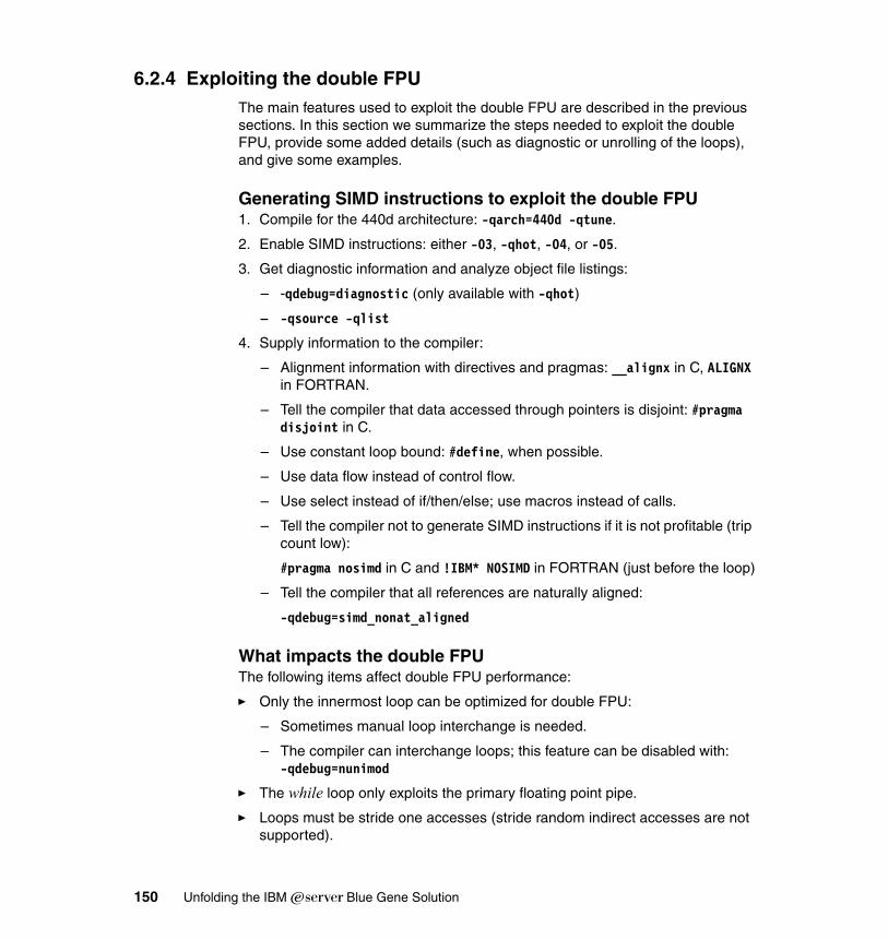
6.2.4 Exploiting the double FPUThe main features used to exploit the double FPU are described in the previous sections. In this section we summarize the steps needed to exploit the double FPU, provide some added details (such as diagnostic or unrolling of the loops), and give some examples.

Generating SIMD instructions to exploit the double FPU1. Compile for the 440d architecture: -qarch=440d -qtune.

2. Enable SIMD instructions: either -03, -qhot, -O4, or -O5.

3. Get diagnostic information and analyze object file listings:

– -qdebug=diagnostic (only available with -qhot)

– -qsource -qlist

4. Supply information to the compiler:

– Alignment information with directives and pragmas: __alignx in C, ALIGNX in FORTRAN.

– Tell the compiler that data accessed through pointers is disjoint: #pragma disjoint in C.

– Use constant loop bound: #define, when possible.

– Use data flow instead of control flow.

– Use select instead of if/then/else; use macros instead of calls.

– Tell the compiler not to generate SIMD instructions if it is not profitable (trip count low):

#pragma nosimd in C and !IBM* NOSIMD in FORTRAN (just before the loop)

– Tell the compiler that all references are naturally aligned:

-qdebug=simd_nonat_aligned

What impacts the double FPUThe following items affect double FPU performance:

� Only the innermost loop can be optimized for double FPU:

– Sometimes manual loop interchange is needed.

– The compiler can interchange loops; this feature can be disabled with: -qdebug=nunimod

� The while loop only exploits the primary floating point pipe.

� Loops must be stride one accesses (stride random indirect accesses are not supported).


� Function calls in loop:

– Try to inline the calls.

� Loop with if statement.

� Pointer and aliasing use.

� Integer operations.

� Assumed shape arrays in FORTRAN 90 (see Example 6-14).

Example 6-14 Assumed-shape arrays in FORTRAN 90 bans SIMD instructions

! Assumed-shape arrays hurt SIMD instruction generationsubroutine simd_off(n, x, y)integer nreal(8) alpha, x(:), y(:)...end

! Replace fortran90 Assumed-shape arrays statements by fortran77 statementssubroutine simd_on(n, x, y)integer nreal(8) alpha, x(*), y(*)...end

Using the diagnostic report and object file listingThe -qdebug=diagnostic compiler option generates a diagnostic report about SIMD instruction generation. The diagnostic report is only available with the high-order transformation module (-qhot). This module can alter the semantic of the code and cannot be set as a default compiler option for many real applications.

We advise enabling diagnostic report for performance-critical routines in order to highlight the SIMD instruction failures. To analyze the generated code and the use of quadword loads and stores, you have to look at the pseudo assembler code within the object file listing.

The diagnostic report provides two types of information on SIMD generation (information on success and information on failure), but it does not contain information about quadword loads and stores instructions. The information on failure allows you to take appropriate actions.

The main information items provided by the diagnostic report are:

1. Information on success:

– (simdizable) [feature][version]


– [feature] further characterizes the simdizable loop:

• misalign (compile time store): This refers to a simdizable loop with misaligned accesses.

• shift( 4 compile time): This refers to a simdizable loop with 4 stream shift inserted. shift means how many misaligned data references were found. This has a performance impact since these loops need to be loaded cross, and then an extra select instruction must be inserted.

• priv: Indicates that the compiler has generated a private variable. priv means a private var was found. In general, it should have no performance impact, but in practice it sometimes does.

• reduct: This means that simdizable loop has a reduction construct. reduct means that a reduction was found. It will be simdized using partial sums, which need to be added up at the end of the loop.

– [version] further characterizes if and why versioned loops were created:

• relative align: Indicates the version for relative alignment. The compiler has generated a test and two versions.

• trip count: Versioned for short runtime trip count.

2. Information on failure allows you to take appropriate actions. The following list contains an explanation of the messages that you might observe:

– In case of misalignment: misalign(...)

• non-natural: Non-naturally aligned accesses

• runtime: runtime alignment

– About the structure of the loop

• irregular loop structure (while-loop)

• contains control flow: if/then/else

• contains function call: function call bans SIMD instructions

• trip count too small

– About dependences: dependence due to aliasing

– About array references

• access not stride one

• mem accesses with unsupported alignment

• contains runtime shift

– About pointer references: non normalized pointer accesses


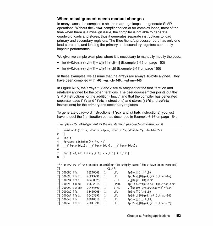
When misalignment needs manual changesIn many cases, the compiler is able to rearrange loops and generate SIMD operations. Without the -qhot compiler option or for complex loops, most of the time when there is a misalign issue, the compiler is not able to generate quadword loads and stores, thus it generates separate instructions to load primary and secondary registers. The Blue Gene/L processor core has only one load-store unit, and loading the primary and secondary registers separately impacts performance.

We give two simple examples where it is necessary to manually modify the code:

� for (i=0;i<n;i++) y[i+1] = x[i+1] + c[i+1] (Example 6-15 on page 153)

� for (i=0;i<n;i++) y[i+1] = x[i+1] + c[i] (Example 6-17 on page 155)

In these examples, we assume that the arrays are always 16-byte aligned. They have been compiled with -03 -qarch=440d -qtune=440.

In Figure 6-15, the arrays x, y and c are misaligned for the first iteration and relatively aligned for the other iterations. The pseudo-assembler points out the SIMD instructions for the addition (fpadd) and that the compiler has generated separate loads (lfd and lfsdx instructions) and stores (stfd and stfsdx instructions) for the primary and secondary registers.

To generate quadword instructions (lfpdx and stfpdx instructions) you just have to peel the first iteration out, as described in Example 6-16 on page 154.

Example 6-15 Misalignment for the first iteration (no quadword instructions)

1 | void add3(int n, double alpha, double *x, double *y, double *c)2 | {3 | int i;4 | #pragma disjoint(*x,*y, *c)5 | __alignx(16,x); __alignx(16,y); __alignx(16,c);6 |7 | for (i=0;i<n;i++) y[i+1] = x[i+1] + c[i+1];8 | }

*** overview of the pseudo-assembler (to simply some lines have been removed)7| CL.47:7| 00008C lfd C8240008 1 LFL fp1=x[]0(gr4,8)7| 000090 lfsdx 7C24399C 1 LFL fp33=x[]0(gr4,gr7,0,trap=16)7| 000094 stfd D8450028 1 STFL y[]0(gr5,40)=fp27| 000098 fpadd 00602018 1 FPADD fp3,fp35=fp0,fp32,fp4,fp36,fcr7| 00009C stfsdx 7C45459C 1 STFL y[]0(gr5,gr8,0,trap=48)=fp347| 0000A0 lfd C8460008 1 LFL fp2=c[]0(gr6,8)7| 0000A4 lfsdx 7C46399C 1 LFL fp34=c[]0(gr6,gr7,0,trap=16)7| 0000A8 lfd C8040018 1 LFL fp0=x[]0(gr4,24)7| 0000AC lfsdx 7C04199C 1 LFL fp32=x[]0(gr4,gr3,0,trap=32)


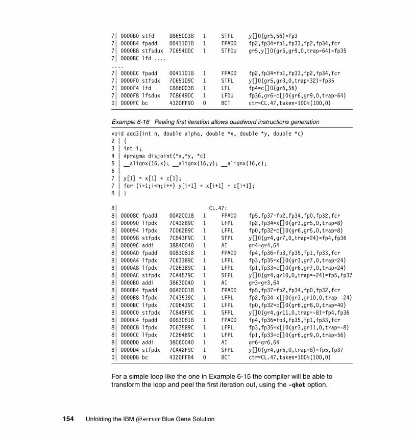
7| 0000B0 stfd D8650038 1 STFL y[]0(gr5,56)=fp37| 0000B4 fpadd 00411018 1 FPADD fp2,fp34=fp1,fp33,fp2,fp34,fcr7| 0000B8 stfsdux 7C654DDC 1 STFDU gr5,y[]0(gr5,gr9,0,trap=64)=fp357| 0000BC lfd ........7| 0000EC fpadd 00411018 1 FPADD fp2,fp34=fp1,fp33,fp2,fp34,fcr7| 0000F0 stfsdx 7C651D9C 1 STFL y[]0(gr5,gr3,0,trap=32)=fp357| 0000F4 lfd C8860038 1 LFL fp4=c[]0(gr6,56)7| 0000F8 lfsdux 7C8649DC 1 LFDU fp36,gr6=c[]0(gr6,gr9,0,trap=64)0| 0000FC bc 4320FF90 0 BCT ctr=CL.47,taken=100%(100,0)

Example 6-16 Peeling first iteration allows quadword instructions generation

void add3(int n, double alpha, double *x, double *y, double *c)2 | {3 | int i;4 | #pragma disjoint(*x,*y, *c)5 | __alignx(16,x); __alignx(16,y); __alignx(16,c);6 |7 | y[1] = x[1] + c[1];7 | for (i=1;i<n;i++) y[i+1] = x[i+1] + c[i+1];8 | }

8| CL.47:8| 00008C fpadd 00A20018 1 FPADD fp5,fp37=fp2,fp34,fp0,fp32,fcr8| 000090 lfpdx 7C432B9C 1 LFPL fp2,fp34=x[]0(gr3,gr5,0,trap=8)8| 000094 lfpdx 7C062B9C 1 LFPL fp0,fp32=c[]0(gr6,gr5,0,trap=8)8| 000098 stfpdx 7C843F9C 1 SFPL y[]0(gr4,gr7,0,trap=24)=fp4,fp368| 00009C addi 38840040 1 AI gr4=gr4,648| 0000A0 fpadd 00830818 1 FPADD fp4,fp36=fp3,fp35,fp1,fp33,fcr8| 0000A4 lfpdx 7C633B9C 1 LFPL fp3,fp35=x[]0(gr3,gr7,0,trap=24)8| 0000A8 lfpdx 7C263B9C 1 LFPL fp1,fp33=c[]0(gr6,gr7,0,trap=24)8| 0000AC stfpdx 7CA4579C 1 SFPL y[]0(gr4,gr10,0,trap=-24)=fp5,fp378| 0000B0 addi 38630040 1 AI gr3=gr3,648| 0000B4 fpadd 00A20018 1 FPADD fp5,fp37=fp2,fp34,fp0,fp32,fcr8| 0000B8 lfpdx 7C43539C 1 LFPL fp2,fp34=x[]0(gr3,gr10,0,trap=-24)8| 0000BC lfpdx 7C06439C 1 LFPL fp0,fp32=c[]0(gr6,gr8,0,trap=40)8| 0000C0 stfpdx 7C845F9C 1 SFPL y[]0(gr4,gr11,0,trap=-8)=fp4,fp368| 0000C4 fpadd 00830818 1 FPADD fp4,fp36=fp3,fp35,fp1,fp33,fcr8| 0000C8 lfpdx 7C635B9C 1 LFPL fp3,fp35=x[]0(gr3,gr11,0,trap=-8)8| 0000CC lfpdx 7C264B9C 1 LFPL fp1,fp33=c[]0(gr6,gr9,0,trap=56)8| 0000D0 addi 38C60040 1 AI gr6=gr6,648| 0000D4 stfpdx 7CA42F9C 1 SFPL y[]0(gr4,gr5,0,trap=8)=fp5,fp370| 0000D8 bc 4320FFB4 0 BCT ctr=CL.47,taken=100%(100,0)

For a simple loop like the one in Example 6-15 the compiler will be able to transform the loop and peel the first iteration out, using the -qhot option.


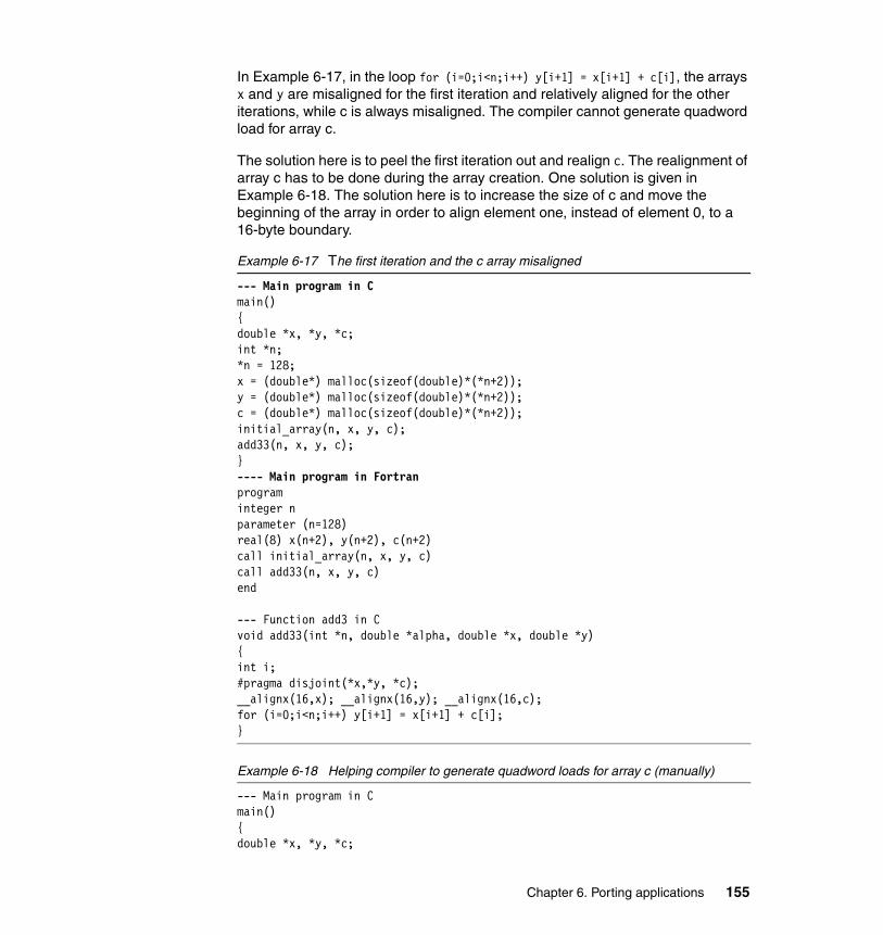
In Example 6-17, in the loop for (i=0;i<n;i++) y[i+1] = x[i+1] + c[i], the arrays x and y are misaligned for the first iteration and relatively aligned for the other iterations, while c is always misaligned. The compiler cannot generate quadword load for array c.

The solution here is to peel the first iteration out and realign c. The realignment of array c has to be done during the array creation. One solution is given in Example 6-18. The solution here is to increase the size of c and move the beginning of the array in order to align element one, instead of element 0, to a 16-byte boundary.

Example 6-17 The first iteration and the c array misaligned

--- Main program in Cmain() {double *x, *y, *c;int *n;*n = 128;x = (double*) malloc(sizeof(double)*(*n+2));y = (double*) malloc(sizeof(double)*(*n+2));c = (double*) malloc(sizeof(double)*(*n+2));initial_array(n, x, y, c);add33(n, x, y, c);}---- Main program in Fortranprogram integer nparameter (n=128)real(8) x(n+2), y(n+2), c(n+2)call initial_array(n, x, y, c)call add33(n, x, y, c)end

--- Function add3 in Cvoid add33(int *n, double *alpha, double *x, double *y){int i;#pragma disjoint(*x,*y, *c);__alignx(16,x); __alignx(16,y); __alignx(16,c);for (i=0;i<n;i++) y[i+1] = x[i+1] + c[i];}

Example 6-18 Helping compiler to generate quadword loads for array c (manually)

--- Main program in Cmain() {double *x, *y, *c;


int *n;*n = 128;x = (double*) malloc(sizeof(double)*(*n+2));y = (double*) malloc(sizeof(double)*(*n+2));c = (double*) malloc(sizeof(double)*(*n+4));c++;initial_array(n, x, y, c);add33(n, x, y, c);}---- Main program in Fortranprogram integer nparameter (n=128)real(8) x(n+2), y(n+2), c(0:n+3)call initial_array(n, x, y, c(1))call add33(n, x, y, c(1))end

--- Function add3 in Cvoid add33(int *n, double *alpha, double *x, double *y){int i;#pragma disjoint(*x,*y, *c);__alignx(16,x); __alignx(16,y); __alignx(16,c+1);y[1] = x[1] + c[0];for (i=1;i<n;i++) y[i+1] = x[i+1] + c[i];}

Unrolling loopsThe compiler is designed to perform unrolling of loops to an adequate depth. Nevertheless, in some cases increasing the unrolling depth can generate more efficient code.

The major benefits of unrolling are:

� Data dependency delays can be reduced or eliminated.

� Loads and stores may be eliminated in successive loop iterations.

� Load overhead may be reduced.

� Larger basic blocks resulting from unrolled loops create more instruction scheduling opportunities (and challenges) for the optimizer.

Loop unrolling can be done by hand or by adding #pragma unroll(X) in C and !IBM* UNROLL(X) directives in FORTRAN before the loop, where X specifies the unrolling depth.


Use XL built-in floating point functions for Blue Gene/LThe XL C/C++ and FORTRAN compilers include a large set of built-in functions that are optimized for the PowerPC architecture.

In addition, on Blue Gene/L, the XL compilers provide a set of built-in functions that are specifically optimized for the double FPU. These built-in functions provide an almost one-to-one correspondence with the SIMD instruction set.

All of the C/C++ and FORTRAN built-in functions operate on complex data types, which have an underlying representation of a two-element array, in which the real part represents the primary element and the imaginary part represents the second element. The input data you provide does not actually need to represent complex numbers: in fact, both elements are represented internally as two real values, and none of the built-in functions actually performs complex arithmetic. A set of built-in functions specially designed to efficiently manipulate complex-type variables is also available.

For a full description of these functions refer to the Blue Gene/L: Application Development, SG24-6745.

We provide an example of the use of built-in functions in C and FORTRAN here (Example 6-19 and Example 6-20). The example creates a custom parallel add function that uses the parallel load and adds built-in functions to add two double floating-point values in parallel and return the result as a complex number.

Example 6-19 Use of built-in functions - C/C++

double _Complex padd(double *x, double *y){double _Complex a,b,c;/* note possibility of alignment trap if (((unsigned int) x) % 32) >= 17) */

a = __lfpd(x); //load x[0] to the primary part of a, x[1] to the secondary part of ab = __lfpd(y); //load y[0] to primary part of b, y[1] to the secondary part of bc = __fpadd(a,b); // the primary part of c = x[0] + y[0]

/* the secondary part of c = x[1] + y[1] */return c;/* alternately: */return __fpadd(__lfpd(x), __lfpd(y)); /* same code generated with optimization

Note: For quadword loads/stores and double FPU instructions, the unrolling depth should be a multiple of two; otherwise, the compiler will unroll on the inferior value. On POWER4 or POWER5, the compile can unroll the loops based on an odd depth according to the programmer’s instruction. On Blue Gene/L, in order to generate SIMD instructions, the compiler forces this to be an even number irrespective of the programmer’s instruction.


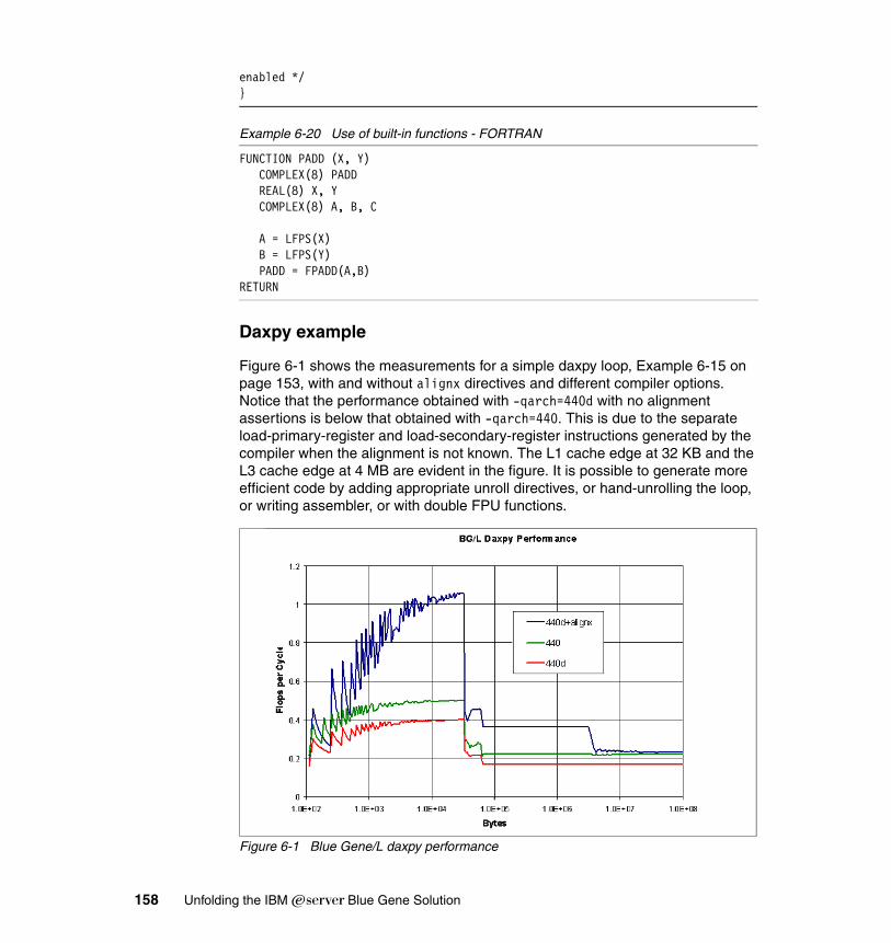
enabled */}

Example 6-20 Use of built-in functions - FORTRAN

FUNCTION PADD (X, Y)COMPLEX(8) PADDREAL(8) X, YCOMPLEX(8) A, B, C

A = LFPS(X)B = LFPS(Y)PADD = FPADD(A,B)

RETURN

Daxpy example

Figure 6-1 shows the measurements for a simple daxpy loop, Example 6-15 on page 153, with and without alignx directives and different compiler options. Notice that the performance obtained with -qarch=440d with no alignment assertions is below that obtained with -qarch=440. This is due to the separate load-primary-register and load-secondary-register instructions generated by the compiler when the alignment is not known. The L1 cache edge at 32 KB and the L3 cache edge at 4 MB are evident in the figure. It is possible to generate more efficient code by adding appropriate unroll directives, or hand-unrolling the loop, or writing assembler, or with double FPU functions.

Figure 6-1 Blue Gene/L daxpy performance


6.2.5 Divide, square root operations, and vector intrinsic functionsThe compiler is capable of generating calls to optimized vector versions of intrinsic functions. These functions are included in the libxlopt.a library within XL FORTRAN and vac C/C++ compilers. These calls are generated by the high-order transformation module (-qhot). Some options, like -qhot=novector or -qstrict, prevent the compiler from calling vector functions.

In many applications, the intrinsic functions can account for an important part of the CPU usage, and calling the vector versions may significantly improve performance. On Blue Gene/L, the number of vector functions available will increase with the releases of the compiler. Therefore, we advise recompiling the program after each major release of the compiler. Unlike the AIX XLF or vac compilers, the number of vector functions available on Blue Gene/L is limited. Only the functions vrec for inverse division, vsqrt for the square root and vrsqst for the inverse square root are implemented in the libxlopt.a library.

Divide and square rootOn Blue Gene/L, the hardware has a reciprocal estimate for the square root (fprsqte instruction) and division (fpre instruction). The precision of these estimates is much more accurate than on other PPC machines, and it allows a Newton iteration scheme to refine the estimate faster than it would the division operation.

In favorable cases, using -O3 -qarch=440d, the compiler will generate a special Newton code based on Blue Gene/L hardware reciprocal estimates for division, square root, and reverse. This results in pipe-lined SIMD instructions that have high performance and may give a huge performance boost for some real applications. A quick glance at the pseudo assembler code allows easy detection of fprsqte or fpre instructions.

The vector vrec, vqsrt and vrsqrt routines, from the libxlopt.a library, also use parallel estimate instructions and Newton's method. For small vectors the call overhead may slow down operations. Today, these routines, calls from -qhot, do not have the same efficiency as the routines from the vector MASS library. In future releases of the compiler, these routines will be the same in both libxlopt.a

Note: You can observe in the daxpy example that the gain from the SIMD instructions is lost when the data only fits in the RAM memory. The memory subsystem does not allow taking advantage of SIMD instructions. Therefore, for applications which do not reuse the data in the cache, we recommend that you not spend a lot of time on SIMD generation.


and libmassv.a. Currently, we recommend linking with the vector MASS library. For more details see “MASS and MASSV libraries” on page 168.

Under -O3 level or with -qarch=440 the compiler will call the standard fdiv instruction and will not take advantage of the Blue Gene/L hardware. For square-root the compiler will call the sqrt or rsqrt functions from the libm.a library. The standard fdiv takes 29 cycles, compared to 14.1 cycle for vdiv and 3.5 cycles for vrec.

6.2.6 Memory managementAs already pointed out, it is important to think about the memory management on a Blue Gene/L system. Even though no application can overtake the physical memory, many performance issues can be identified based on a good knowledge of the memory subsystem. The memory subsystem of Blue Gene/L nodes has specific characteristics and limitations that the programmer should know about.

Memory management is not the same on the I/O node and the compute nodes. On both nodes the virtual address space exactly matches the real address space. TLB misses are handled by the kernel software. On the I/O node the memory pages are 4 KB in size and the processor core can address 256 KB without TLB miss. On the compute node the size of the memory page is 256 MB; therefore, there are no TLB misses on the compute nodes.

In the following section we explain in detail all the components of the Blue Gene/L node memory subsystem. It is useful for a programmer who wants to port and tune applications on Blue Gene/L to understand the behavior of each component of the memory subsystem. We point out the main traps which must be avoided in this section.

Memory addressingFrom the point of view of the Compute Node Kernel, application data is categorized as one the following types:

data Initialized static and common variables

bss Uninitialized static and common variables

heap Controlled allocatable arrays

stack Controlled automatic arrays and variables

Figure 6-2 describes the memory addressing for an executable. The text section starts at address 0. The heap section begins from the bottom, after the data and bss sections, and the stack section starts from the top, at address 1feaa93c (around 510.6 MB) in coprocessor mode and at the address feea93c (around


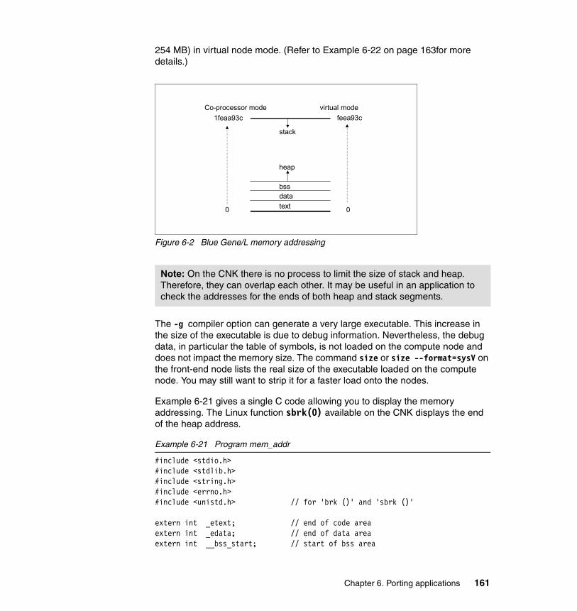
254 MB) in virtual node mode. (Refer to Example 6-22 on page 163for more details.)

Figure 6-2 Blue Gene/L memory addressing

The -g compiler option can generate a very large executable. This increase in the size of the executable is due to debug information. Nevertheless, the debug data, in particular the table of symbols, is not loaded on the compute node and does not impact the memory size. The command size or size --format=sysV on the front-end node lists the real size of the executable loaded on the compute node. You may still want to strip it for a faster load onto the nodes.

Example 6-21 gives a single C code allowing you to display the memory addressing. The Linux function sbrk(0) available on the CNK displays the end of the heap address.

Example 6-21 Program mem_addr

#include <stdio.h>#include <stdlib.h>#include <string.h>#include <errno.h>#include <unistd.h> // for 'brk ()' and 'sbrk ()'

extern int _etext; // end of code areaextern int _edata; // end of data areaextern int __bss_start; // start of bss area

Note: On the CNK there is no process to limit the size of stack and heap. Therefore, they can overlap each other. It may be useful in an application to check the addresses for the ends of both heap and stack segments.

datatext

bss

heap

stack

virtual modeCo-processor mode1feaa93c feea93c

0 0


extern int _end; // end of bss area

unsigned long heapsize () { return (unsigned long) sbrk (0) - (unsigned long) & _end; }

void * gotostack () { long st[SZ*SIZE]; st[0]=123456; printf ("\nstart of stack address %9lx\n", &st[SZ*SIZE-1]); printf ("end of stack address %9lx\n\n", st); }

#define SIZE 1024*256 // 1 MB of long// #define SZ 248 // virtual mode#define SZ 500 // co-processor mode

int initialized = 123; // goes to data areaint uninitialized; // goes to bssint main (int argc, char * argv []){int loop;long long_integer;long * heap_array;long * heap_array0;

errno=0;

if ((heap_array0 = (long *) malloc (SZ*SIZE*sizeof(long_integer))) == NULL)printf("error, could not allocate\n");if( errno !=0 ){printf ("malloc errno : %d\n",errno); errno=0; }

if ((heap_array = (long *) malloc (SIZE*sizeof(long_integer))) == NULL)printf("error, could not allocate\n");if( errno !=0 ){printf ("malloc errno : %d\n",errno); errno=0;}

printf ("Memory mapping\n\n");printf ("heapsize function address %9lx\n", heapsize);printf ("printf function address %9lx\n", printf);printf ("end of code address %9lx\n", &_etext);printf ("variable initialized address %9lx\n", &initialized);printf ("end of data address %9lx\n", &_edata);printf ("start of bss address %9lx\n", &__bss_start);printf ("variable uninitialized address %9lx\n", &uninitialized);printf ("end of bss address %9lx\n", &_end);printf ("start of heap address %9lx\n", heap_array0);


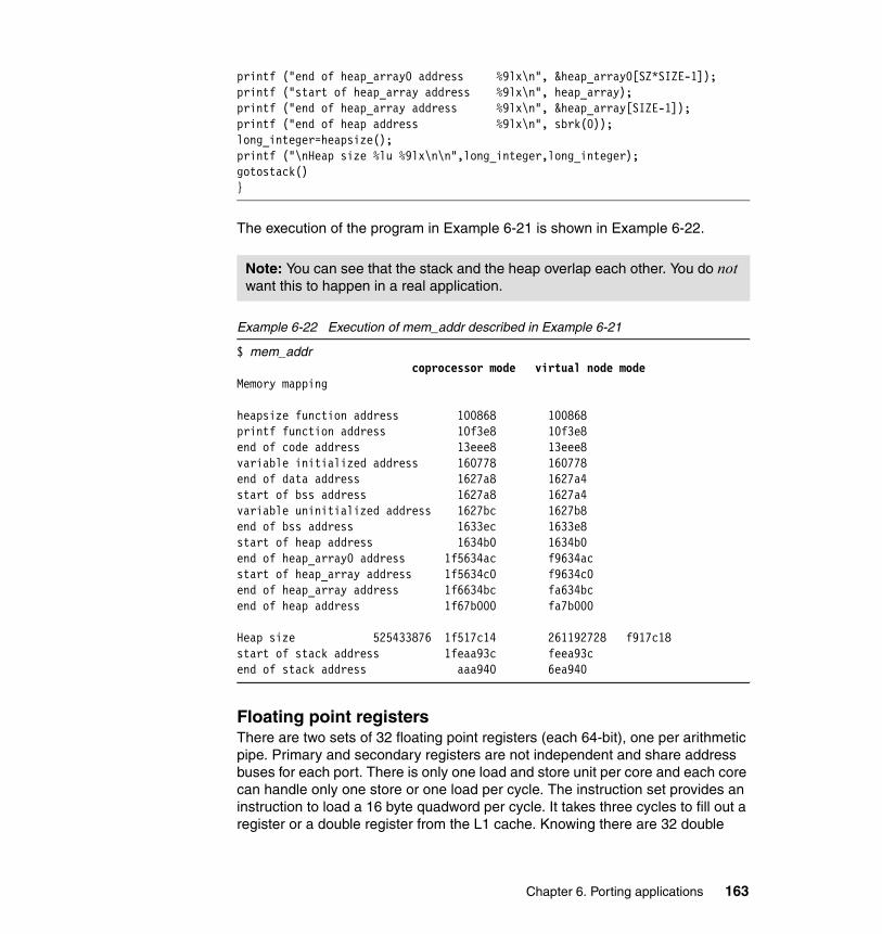
printf ("end of heap_array0 address %9lx\n", &heap_array0[SZ*SIZE-1]);printf ("start of heap_array address %9lx\n", heap_array);printf ("end of heap_array address %9lx\n", &heap_array[SIZE-1]);printf ("end of heap address %9lx\n", sbrk(0));long_integer=heapsize();printf ("\nHeap size %lu %9lx\n\n",long_integer,long_integer);gotostack()}

The execution of the program in Example 6-21 is shown in Example 6-22.

Example 6-22 Execution of mem_addr described in Example 6-21

$ mem_addrcoprocessor mode virtual node mode

Memory mapping

heapsize function address 100868 100868printf function address 10f3e8 10f3e8end of code address 13eee8 13eee8variable initialized address 160778 160778end of data address 1627a8 1627a4start of bss address 1627a8 1627a4variable uninitialized address 1627bc 1627b8end of bss address 1633ec 1633e8start of heap address 1634b0 1634b0end of heap_array0 address 1f5634ac f9634acstart of heap_array address 1f5634c0 f9634c0end of heap_array address 1f6634bc fa634bcend of heap address 1f67b000 fa7b000

Heap size 525433876 1f517c14 261192728 f917c18start of stack address 1feaa93c feea93cend of stack address aaa940 6ea940

Floating point registersThere are two sets of 32 floating point registers (each 64-bit), one per arithmetic pipe. Primary and secondary registers are not independent and share address buses for each port. There is only one load and store unit per core and each core can handle only one store or one load per cycle. The instruction set provides an instruction to load a 16 byte quadword per cycle. It takes three cycles to fill out a register or a double register from the L1 cache. Knowing there are 32 double

Note: You can see that the stack and the heap overlap each other. You do not want this to happen in a real application.


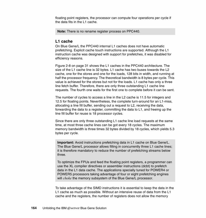
floating point registers, the processor can compute four operations per cycle if the data fits in the L1 cache.

L1 cacheOn Blue Gene/L the PPC440 internal L1 caches does not have automatic prefetching. Explicit cache touch instructions are supported. Although the L1 instruction cache was designed with support for prefetches, it was disabled for efficiency reasons.

Figure 2-8 on page 31 shows the L1 caches in the PPC440 architecture. The size of the L1 cache line is 32 bytes. L1 cache has two buses towards the L2 cache, one for the stores and one for the loads, 128 bits in width, and running at half the processor frequency. The theoretical bandwidth is 8 bytes per cycle. This value is achieved for the stores but not for the loads. L1 cache has only a three line fetch buffer. Therefore, there are only three outstanding L1 cache line requests. The fourth one waits for the first one to complete before it can be sent.

The number of cycles to access a line in the L2 cache is 11.5 for integers and 12.5 for floating points. Nevertheless, the complete turn-around for an L1-miss, allocating a line fill buffer, sending out a request to L2, receiving the data, forwarding the data to a register, committing the data to L1, and freeing up the line fill buffer for reuse is 18 processor cycles.

Since there are only three outstanding L1 cache line load requests at the same time, at most three cache lines can be got every 18 cycles. The maximum memory bandwidth is three times 32 bytes divided by 18 cycles, which yields 5.3 bytes per cycle.

To take advantage of the SIMD instructions it is essential to keep the data in the L1 cache as much as possible. Without an intensive reuse of data from the L1 cache and the registers, the number of registers does not allow the memory

Note: There is no rename register process on PPC440.

Important: Avoid instructions prefetching data in L1 cache on Blue Gene/L. The Blue Gene/L processor allows filling in concurrently three L1 cache lines; it is therefore mandatory to reduce the number of prefetching streams below three.

To optimize the FPUs and feed the floating point registers, a programmer can use the XL compiler directives or assembler instructions (dcbt) to prefetch data in the L1 data cache. The applications specially tuned for POWER4 or POWER5 processors taking advantage of four or eight prefetching engines will choke the memory subsystem of the Blue Gene/L processor.


subsystem to feed the double FPU and provide two multiply-addition operations per cycle.

In the worst case, SIMD instructions can hurt the global performance of the application. For that reason we advise disabling the SIMD instructions in the porting phase by compiling with -qarch=440, then recompiling the code with -qarch=440d and analyzing the performance impact of SIMD instructions. The analysis should be done with a data set and a number of processorsthat is realistic in terms of memory usage.

L2 cacheBlue Gene/L L2 cache, shown in Figure 2-7 on page 29, is the hardware layer providing the link between the embedded cores and Blue Gene/L devices such as the 4 MB L3-eDRAM and the 16 kB SRAM. The 2 KB L2 cache line is 128 Bytes in size. Each L2 cache is connected to one processor core. They are fully associative and are coherent. Basically, they act as prefetch and write-back buffers for the L1 data cache.

The L2 design and architecture was created to provide optimal support for the PC440 cores for scientific applications. Thus, a logic for automatic sequential stream detection and prefetching to the L2 has been added. The logic is optimized to perform best on sequential streams with increasing addresses. The L2 boosts the overall performance for almost any application and does not require any special software provisions. It autonomously detects streams, issues the prefetch requests, and keeps the prefetched data coherent.

Careful programming will help to achieve latency/bandwidth results very close to the theoretical limits (5.3 bytes per cycle) dictated by the PPC440 core. The L2 accelerates memory accesses for one up to seven sequential streams. More parallel streams could be supported in theory, but require careful data layout and instruction scheduling for only marginal acceleration. (Although more than seven streams are supported by the hardware, this mode of operation is not recommended.)

L3 cacheThe 4 MB L3 cache is described in 2.2.3, “Memory system overview” on page 31. The line size is 128 bytes. Both banks are directly accessed by the two processor

Important:

� The otpimization of the applications has to be based on the 32 KB of the L1 cache.

� The benefits of the SIMD instructions might be cancelled out if data does not fit in L1 cache.


cores and the gigabit network, only on the I/O node. There are three write queues and three read queues. The read queues directly access both banks.

There are three write queues, each four 32-byte entries deep. Each write queue can deposit up to one request per cycle into the four entry deep write buffer. The write buffer can accept one request from every write queue in every cycle (for a total of up to three per cycle) to any location in the four lines. All three 32-byte requests can, for example, be to a single line in the write buffer or to three different lines in the write buffer. This performance is possible provided valid lines are established in the write buffer and the incoming requests match the address of the write lines. If a request arrives at the write buffer and is not matching an address of the established lines, a new line has to be allocated. A new line can be allocated if there is a free line in the buffer available. The buffer can allocate a new line every two cycles.

The transition of a valid line becoming free takes between four and six cycles on cache hit, and more for a miss. The transition is triggered by either a read after write conflict, the line containing 128 Bytes of valid data, or a write buffer fill level threshold being crossed. Several lines can make the transition in parallel.

On the compute node, in sequential access, four 32-byte write requests (one line) from each processor core can be completed in six cycles. In random access each write request addresses a new line, and four write requests take between 15 and 18 cycles in virtual node mode and around 14 cycles in coprocessor mode.

DDR (Double Data RAM) memory architecture The theoretical memory bandwidth on a Blue Gene/L node to transfer a 128-byte line from the external DDR memory to the L3 cache is 16 cycles. Nevertheless, this bandwidth can only be sustained with sequential access. Random access can reduce bandwidth significantly.

Important: Random access can divide the write sustained bandwidth of the L3 cache by a factor of three on compute nodes and more on I/O nodes.


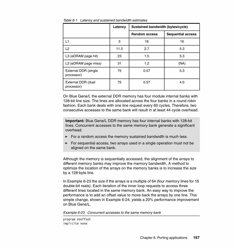
Table 6-1 Latency and sustained bandwidth estimates

On Blue Gene/L the external DDR memory has four module internal banks with 128-bit line size. The lines are allocated across the four banks in a round robin fashion. Each bank deals with one line request every 60 cycles. Therefore, two consecutive accesses to the same bank will result in at least 44 cycle overhead.

Although the memory is sequentially accessed, the alignment of the arrays to different memory banks may improve the memory bandwidth. A method to optimize the location of the arrays on the memory banks is to increase the size by a 128-byte line.

In Example 6-23 the size if the arrays is a multiple of 64 (four memory lines for 16 double-bit reals). Each iteration of the inner loop requests to access three different lines located in the same memory bank. An easy way to improve the performance is to add an offset value to move back the arrays by one line. This simple change, shown in Example 6-24, yields a 20% performance improvement on Blue Gene/L.

Example 6-23 Concurrent accesses to the same memory bank

program nooffsetimplicite none

Latency Sustained bandwidth (bytes/cycle)

Random access Sequential access

L1 3 16 16

L2 11.5 2.7 5.3

L3 (eDRAM page hit) 23 1.5 5.3

L3 (eDRAM page miss) 31 1.2 (NA)

External DDR (single processor)

75 0.57 5.3

External DDR (dual processor)

75 0.57 4.0

Important: Blue Gene/L DDR memory has four internal banks with 128-bit lines. Concurrent accesses to the same memory bank generate a significant overhead.

� For a random access the memory sustained bandwidth is much less.

� For sequential access, two arrays used in a single operation must not be aligned on the same bank.


integer nparameter (n=12800000)real(8) x(n), y(n), w(n)integer i,jinteger(8) time0, time1, rts_get_timebase

call rand_seedcall rand_number(x)call rand_number(y)call rand_number(w)do j=1,1000

call dummy()time0 = rts_get_timebase()do j=1,n

x(1) = x(1) + y(1)*w(1)enddotime1 = rts_get_timebase()

enddowrite(6,*) ‘total time in seconds : ‘, (time1-tim0)/(700.D6)end

Example 6-24 Offset the arrays the memory banks vs. Example 6-23

program offsetimplicite noneinteger n, offsetparameter (n=12800000, offset=16)real(8) x(n+offset), y(n+2*offset), w(n)....same as Example 6-23 on page 167

6.2.7 Math librariesThis section provides information about the math libraries currently available on Blue Gene/L. The number of math libraries will increase with the marketing of Blue Gene/L. We recommend using the math libraries as much as possible.

MASS and MASSV librariesThe mathematical acceleration subsystem (MASS) library provides high performance versions of a subset of FORTRAN intrinsic functions. Compared to the standard mathematical library, the results may not be bit-to-bit identical. Nevertheless, MASS results are generally sufficiently accurate for most applications; only people using special IEEE rounding options may chose not to use it.


The MASS library can be downloaded from:

http://www-306.ibm.com/software/awdtools/mass/

There are two basic types of function available for each operation, a single instance function (libmass.a) and a vector function (libmassv.a). The single instance function simply replaces the libm.a call with a MASS library call. The vector function is used to produce a vector of results given a vector operand. The vector MASS functions may require coding changes while the single instance functions do not.

To enable the MASS functions the application must be linked with the libmass.a library for the single instance functions and with the ibmassv.a library for vector functions. Ask your system administrator for the location of mass libraries. To avoid errors during the link due to multiple definitions, add to the option:

-Wl,--allow-multiple-definition

The vector functions are the same name and arguments as the vector intrinsic functions within the libxlopt.a library within XL compiler, described in 6.2.5, “Divide, square root operations, and vector intrinsic functions” on page 159.

An example using the MASS library with FORTRAN code follows. This code would be rather expensive using the standard cos and sin functions and may be replaced using the vector MASS reciprocal approximation function vsincos (See Example 6-25).

Example 6-25 How to use a vector mass function

! Original codereal(8) x(*), y(*), z’*)...do i=1,nx(i) = sin(z(i))y(i) = sin(z(i))

enddo! With MASSV library the loop can be replaced by the function vsincos! call vsincos(x, y, z, n)

All the functions are written in C and compiled for Blue Gene/L double FPU. The performance gain compared to standard functions is very high and will be improved in the future. Table 6-2 presents some performance (in clock cycles) on Blue Gene/L.


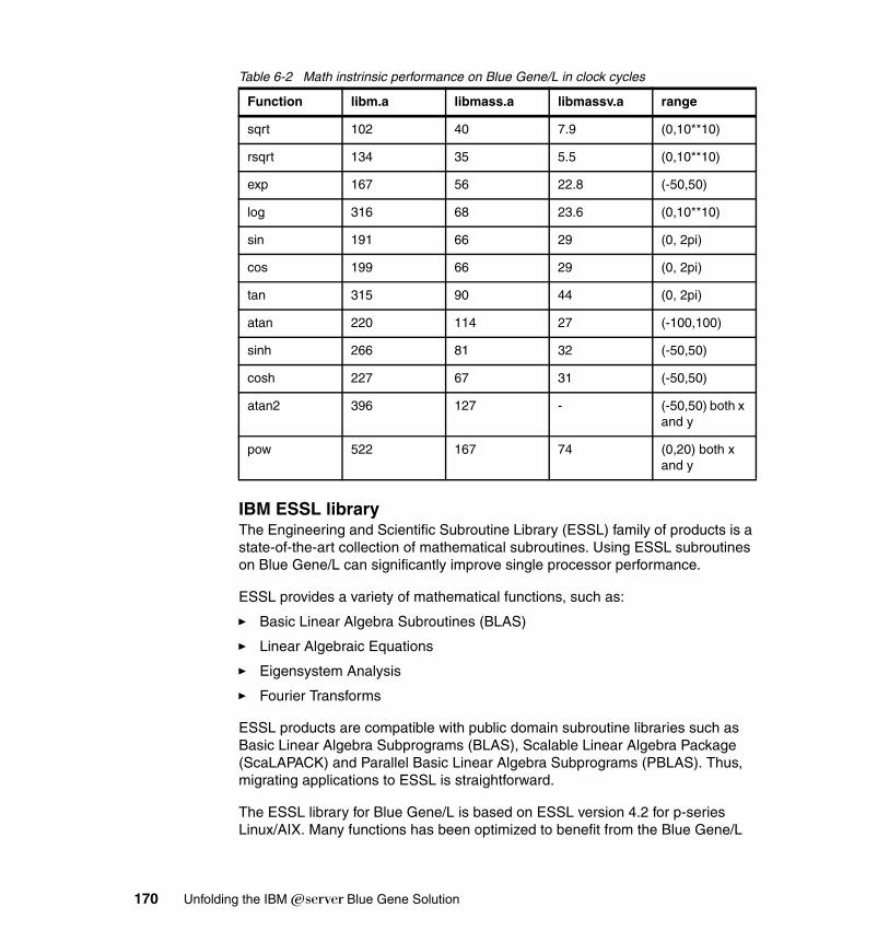
Table 6-2 Math instrinsic performance on Blue Gene/L in clock cycles

IBM ESSL libraryThe Engineering and Scientific Subroutine Library (ESSL) family of products is a state-of-the-art collection of mathematical subroutines. Using ESSL subroutines on Blue Gene/L can significantly improve single processor performance.

ESSL provides a variety of mathematical functions, such as:

� Basic Linear Algebra Subroutines (BLAS)

� Linear Algebraic Equations

� Eigensystem Analysis

� Fourier Transforms

ESSL products are compatible with public domain subroutine libraries such as Basic Linear Algebra Subprograms (BLAS), Scalable Linear Algebra Package (ScaLAPACK) and Parallel Basic Linear Algebra Subprograms (PBLAS). Thus, migrating applications to ESSL is straightforward.

The ESSL library for Blue Gene/L is based on ESSL version 4.2 for p-series Linux/AIX. Many functions has been optimized to benefit from the Blue Gene/L

Function libm.a libmass.a libmassv.a range

sqrt 102 40 7.9 (0,10**10)

rsqrt 134 35 5.5 (0,10**10)

exp 167 56 22.8 (-50,50)

log 316 68 23.6 (0,10**10)

sin 191 66 29 (0, 2pi)

cos 199 66 29 (0, 2pi)

tan 315 90 44 (0, 2pi)

atan 220 114 27 (-100,100)

sinh 266 81 32 (-50,50)

cosh 227 67 31 (-50,50)

atan2 396 127 - (-50,50) both x and y

pow 522 167 74 (0,20) both x and y


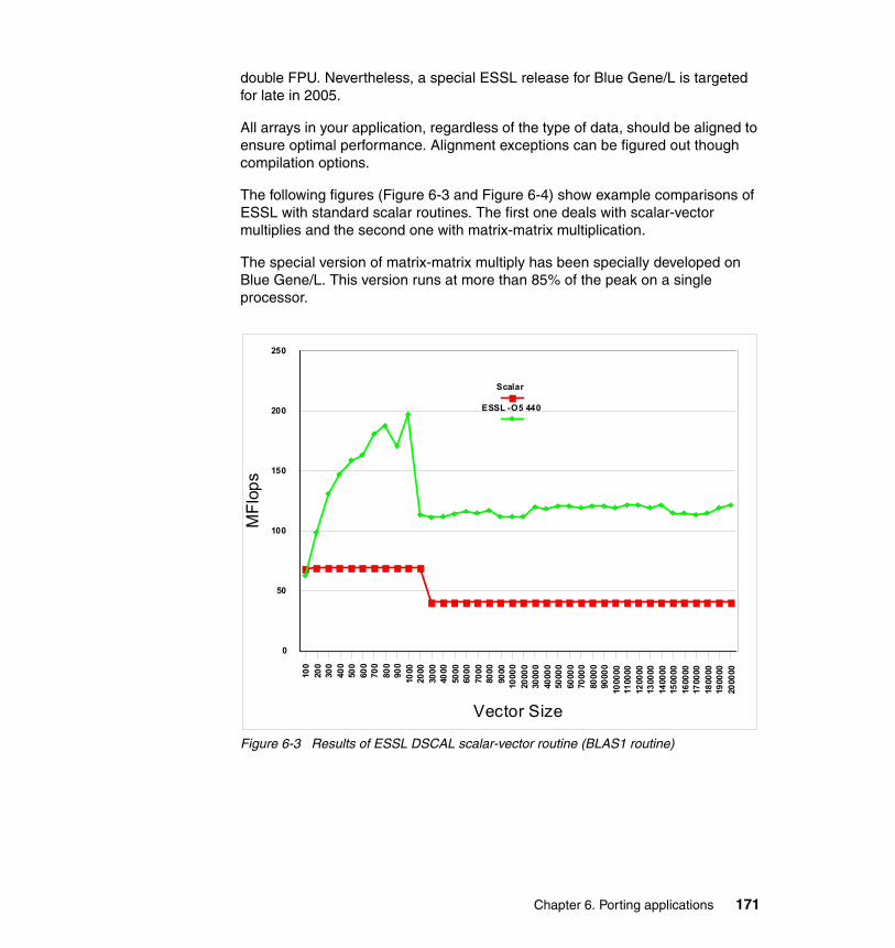
double FPU. Nevertheless, a special ESSL release for Blue Gene/L is targeted for late in 2005.

All arrays in your application, regardless of the type of data, should be aligned to ensure optimal performance. Alignment exceptions can be figured out though compilation options.

The following figures (Figure 6-3 and Figure 6-4) show example comparisons of ESSL with standard scalar routines. The first one deals with scalar-vector multiplies and the second one with matrix-matrix multiplication.

The special version of matrix-matrix multiply has been specially developed on Blue Gene/L. This version runs at more than 85% of the peak on a single processor.

Figure 6-3 Results of ESSL DSCAL scalar-vector routine (BLAS1 routine)

100

200

300

400

500

600

700

800

900

1000

2000

3000

4000

5000

6000

7000

8000

9000

1000

020

000

3000

040

000

5000

060

000

7000

080

000

9000

010

0000

1100

0012

0000

1300

0014

0000

1500

0016

0000

1700

0018

0000

1900

0020

0000

Vector Size

0

50

100

150

200

250

MFl

ops

Scalar

ESSL -O5 440


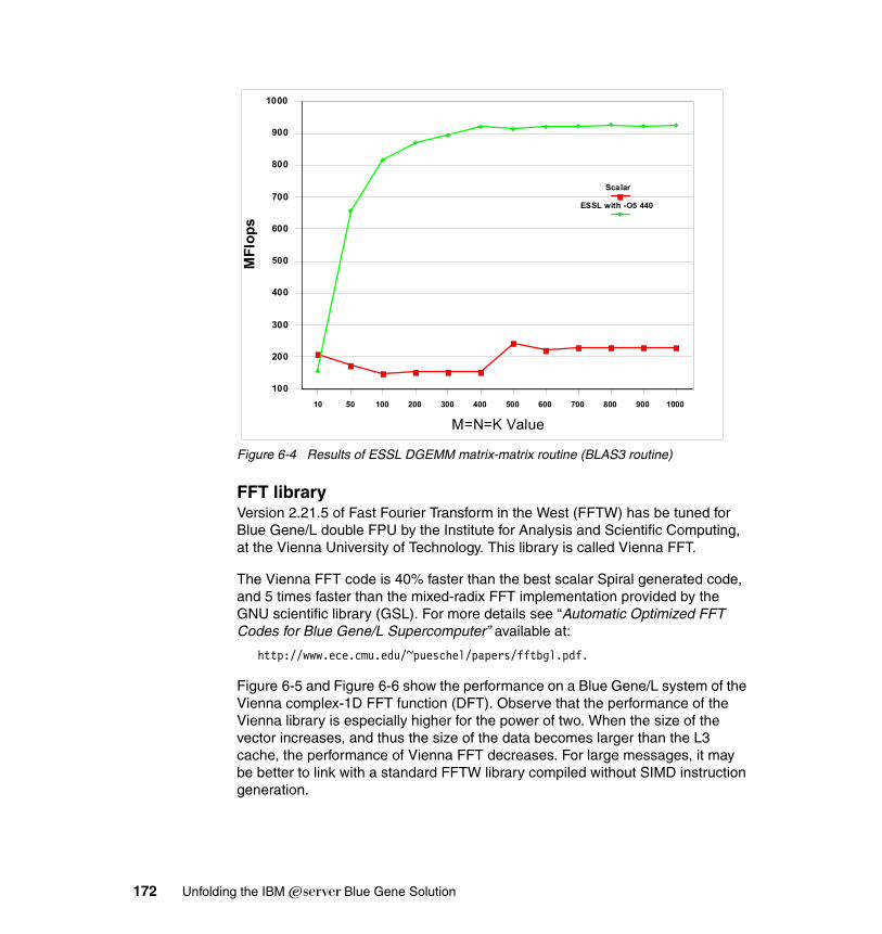
Figure 6-4 Results of ESSL DGEMM matrix-matrix routine (BLAS3 routine)

FFT libraryVersion 2.21.5 of Fast Fourier Transform in the West (FFTW) has be tuned for Blue Gene/L double FPU by the Institute for Analysis and Scientific Computing, at the Vienna University of Technology. This library is called Vienna FFT.

The Vienna FFT code is 40% faster than the best scalar Spiral generated code, and 5 times faster than the mixed-radix FFT implementation provided by the GNU scientific library (GSL). For more details see “Automatic Optimized FFT Codes for Blue Gene/L Supercomputer” available at:

http://www.ece.cmu.edu/~pueschel/papers/fftbgl.pdf.

Figure 6-5 and Figure 6-6 show the performance on a Blue Gene/L system of the Vienna complex-1D FFT function (DFT). Observe that the performance of the Vienna library is especially higher for the power of two. When the size of the vector increases, and thus the size of the data becomes larger than the L3 cache, the performance of Vienna FFT decreases. For large messages, it may be better to link with a standard FFTW library compiled without SIMD instruction generation.

10 50 100 200 300 400 500 600 700 800 900 1000

M=N=K Value

100

200

300

400

500

600

700

800

900

1000

MFl

ops

Scalar

ESSL with -O5 440


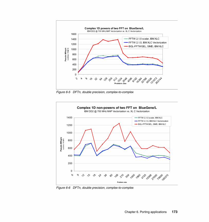
Figure 6-5 DFTn, double precision, complex-to-complex

Figure 6-6 DFTn, double precision, complex-to-complex

Complex 1D powers of two FFT on BlueGene/LIBM DD2 @ 700 MHz MAP Vectorization vs. XL C Vectorization

0

200

400

600

800

1000

1200

1400

1600

2 4 8 16 32 64 128

256

512

1024

2048

4096

8192

1638

432

76865

536

1310

72

2621

44

Problem size

Pseu

do M

flop/

sru

ntim

e / N

ld N

FFTW 2,1,5 scalar, IBM XLCFFTW 2,1,5, IBM XLC Vectorization BGL-FFTWGEL, SIMD, IBM XLC

Complex 1D non-powers of two FFT on BlueGene/LIBM DD2 @ 700 MHz MAP Vectorization vs. XL C Vectorization

0

200

400

600

800

1000

1200

1400

6 9 12 15 18 24 36 80 108

210

504

1000

1960

4725

1036

827

000

7560

0

1653

75

Problem size

Pseu

do M

flop/

sru

ntim

e / N

ld N

FFTW 2,1,5 scalar, IBM XLCFFTW 2,1,5, IBM XLC Vectorization BGL-FFTWGEL, SIMD, IBM XLC


6.2.8 Performance measurementThis section explains how to measure the performance on Blue Gene/L compute nodes.

Time functions The majority of the standard time functions are available on Blue Gene/L compute nodes: gettimeofday(), time(), times(), getrusage(), and so forth. It may be necessary to change some time functions to take into account the features on the Compute Node Kernel.

During the porting step you can encounter some issues due to either the implementation of the CNK features or some features that have yet to be fixed. Some issues we faced during application porting were the following:

� Elapsed time is equal to CPU and the system is equal to 0. Moreover, there are no page faults. You can call getrusage(), which displays information about how the resources are used by the process, but the values that it returns are meaningless.

� The time function reports seconds since the partition was booted, instead of seconds after the reference time. This issue may be fixed in a future release.

� The sysconf(_SC_CLK_TCK) subroutine determines the number of clock ticks per second. All time values reported by the time functions are measured in terms of the number of clock ticks used. The times function on Blue Gene/L provides correct time values, but we noticed that sysconf can report a wrong number of clock ticks. This issue may be fixed in a future release.

Blue Gene/L runtime provides some functions to get information about the compute node. For more details, refer to Appendix B, “BG/L runtime system calls” on page 331. The function rts_get_timetable() returns the number of cycles since the partition was booted. This function can be used for timing. The number of cycles is converted to seconds using the processor frequency (700 MHz).

Example 6-26 shows how to get the elapsed and cpu time, in seconds, using the rst_get_timetable() function in both C and FORTRAN.

Note: On Blue Gene/L, we recommend validating the time functions with small test cases before running the real application. We recommend that you use either gettimeofday() or rts_get_timetable().


Example 6-26 how to use rts_get_timetable in FORTRAN and C

--- in Fortran...integer(8) rts_get_timetablereal(8) time, time1, frequency...frequency = 700.D6time = rts_get_timetable()...time1 = rts_get_timetable()write(6,*)’Total time’,(time1-time)/frequencyend

--- in C#include <rts.h> /* header for rts_get_timetable */...#define frequency 700000000double time, time1...time = (double) rts_get_timetable();...time1 = (double) rts_get_timetable();time1 = (time1 - time)/frequency;printf(“Total time %f \n”,time1);

The profiling fileOn Blue Gene/L the application can be compiled with the standard -p or -pg options to produce an execution profile. Nevertheless, currently the -p or -pg mechanism is only partly ported. The function list and the call numbers are correct but the timing field is meaningless. This issue should be fixed.

In complement of standard profiling options, blrts compiler for Blue Gene/L provides a specific option -qdebug=function_trace or -qxflag=function_trace intersect two functions __function_trace_enter and __function_trace_exit at the beginning and the exit of each function of the applications. This function can be used to define your own profiling tools. All the details are given in 6.5.2, “Instrumenting function entry and exit” on page 196.

Blue Gene/L ASIC hardware countersThese topics are covered in more detail in 5.4.4, “BG/L hardware counters” on page 118 and Appendix G, “Hardware counters” on page 369.


6.3 Porting parallel applicationsWhen porting parallel applications to Blue Gene/L, several areas need to be considered:

� The parallel programming model

� The supported MPI features

� Special behavior of the MPI implementation on Blue Gene/L

� Performance and scaling issues

In this section, we cover each of these areas. Chapter 7, “Massively parallel tuning” on page 207 contains further material on MPI performance and scaling.

6.3.1 The BG/L programming modelBlue Gene/L has a distributed memory system and uses explicit message passing to communicate between tasks running on different nodes. Neither OpenMP nor thread parallelism is supported. If your application uses any of these forms of shared memory parallelism, it needs to be converted to the message passing model in order to use it on Blue Gene/L.

Message Passing Interface (MPI) is the supported message passing standard. MPI is the industry standard for message passing. Further information on MPI can be found at:

http://www.mpi-forum.org/

If your code uses other message passing libraries, you have to either change the message passing calls to MPI, or use an intermediate layer that maps your library’s calls onto MPI.

Note: Even in virtual node mode, the two tasks running on the two CPUs in a BG/L chip are doing message passing to communicate with each other. However, they do not use the torus network; instead, they use a memory area in the chip’s scratchpad memory. This is similar to the shared-memory MPI communication that takes place between tasks within a pSeries SMP node (where inter-node communication uses the interconnect like the eServer High Performance Switch).


6.3.2 MPI features supported on BG/LThe current MPI implementation on Blue Gene/L supports the MPI Version 1.2 standard. This level comprises everything in the MPI Version 1.1 standard document1.

A subset of the MPI Version 2 features is supported, and work is in progress to add some additional capabilities to the BG/L implementation. With regard to porting applications, it is important to understand the following limitations of the current MPI library:

� MPI2 process creation and management are not supported.

� MPI2 one-sided communications are not supported.

� The MPI library is not thread-compliant in the MPI2 sense.

The MPI_Init_Thread function is available, but it will always return MPI_THREAD_SINGLE as the provided argument, regardless of the desired level of thread support that’s passed in as the required argument.

� MPI2 I/O is not supported yet. This feature is currently being developed.

Due to the distributed nature of the I/O infrastructure, MPI-IO is important for a portable mechanism to do I/O on the Blue Gene/L system: there are many I/O nodes which individually only provide limited I/O capabilities. This issue is discussed in more detail in 6.4, “I/O operations” on page 191.

When starting applications on Blue Gene/L, there are some additional details that need to be considered:

� Only executables can be started. Shell scripts are not supported.

The microkernel running on the compute nodes does not provide any mechanisms for a command interpreter or shell. So if your application consists of a number of shell scripts that control its workflow, this will need to be adapted. If you start your application with the mpirun command, you cannot start the main shell script with mpirun, but rather have to run the scripts on the front-end node and only call mpirun at the innermost shell script level where the main application binary is called.

� Launching an application on Blue Gene/L is done in the single program, multiple data (SPMD) model. Within one run, you cannot load one executable onto a subset of the compute nodes and a different executable onto another subset of the compute nodes. If you need some sort of multiple program, multiple data (MPMD) functionality, you can build that into your code by a

1 MPI - A Message Passing Interface Standard. Message Passing Interface Forum. June 12, 1995. and the additional features and clarifications in chapter 3 of the MPI Version 2.0 standard document, MPI-2 - Extensions to the Message Passing Interface. Message Passing Interface Forum. July 18, 1997.


clause similar to the following. This shifts the multiple program feature from the main program level into the subprogram level:

IF (myrank==something) THENCALL some_subprogram(some_args)

ELSECALL another_subprogram(some_other_args)

END IF

This way you can load a single executable onto all nodes, which then branches into different subprograms depending on the local MPI rank.

Apart from these limitations, the MPI library on Blue Gene/L provides all the usual MPI functionality. Users should not have any difficulties porting programs that just contain some basic MPI_Send and MPI_Recv calls. However, in more complex situations there may be some semantic subtleties that you need to understand. In 6.3.3, “The BG/L MPI implementation” on page 178 we discuss some of the implementation details that may cause an MPI program on Blue Gene/L to behave differently than it does on other platforms.

6.3.3 The BG/L MPI implementationThe MPI implementation on Blue Gene/L is derived from the MPICH2 implementation of the Mathematics and Computer Science Division (MCS) at Argonne National Laboratory. Additional information can be obtained from:

http://www-unix.mcs.anl.gov/mpi/mpich/

To support the Blue Gene/L hardware, the following additions and modifications have been made to the MPICH2 software architecture (see Figure 6-7):

� A bgl driver has been added underneath the MPICH2 Abstract Device Interface (ADI).

� Three types of glue code are provided for (some of) the MPI collectives; one for each of the three networks that can be used for MPI communication on Blue Gene/L:

– torus for the torus network

– tree for the collective network

– GI for the barrier (global interrupt) network

� A bgltorus variant for MPICH2’s process management interface.


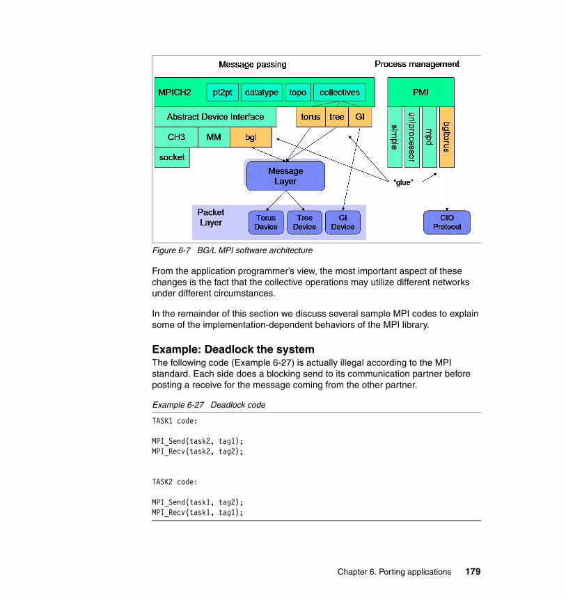
Figure 6-7 BG/L MPI software architecture

From the application programmer’s view, the most important aspect of these changes is the fact that the collective operations may utilize different networks under different circumstances.

In the remainder of this section we discuss several sample MPI codes to explain some of the implementation-dependent behaviors of the MPI library.

Example: Deadlock the systemThe following code (Example 6-27) is actually illegal according to the MPI standard. Each side does a blocking send to its communication partner before posting a receive for the message coming from the other partner.

Example 6-27 Deadlock code

TASK1 code:

MPI_Send(task2, tag1);MPI_Recv(task2, tag2);

TASK2 code:

MPI_Send(task1, tag2);MPI_Recv(task1, tag1);


In general, this has a high probability to deadlock the system. Obviously, you should not program this way, and you should make sure that your code conforms to the MPI specification. You can achieve this by either changing the order of sends and receives, or by using non-blocking communication calls (see Example 6-28).

The MPI implementation on Blue Gene/L was designed to avoid a deadlock in situations like the one just described. The runtime system will try to avoid deadlocks by allocating additional memory to deal with messages that arrive unexpectedly (for example, before a receive has been posted on the local task). It will eventually run out of memory, in which case it will stop the application with an error message.

So while you certainly should not rely on the runtime system to correctly handle non-conforming MPI code, it is easier to debug such situations when you get a runtime error message than trying to detect a deadlock and trace it back to its root cause.

Example: Forcing MPI to allocate too much memoryHere is a slightly different example, in which one task sends a number of messages to a second task, but the messages are received in the reverse order at the sender side (Example 6-28).

Example 6-28 Forcing MPI to allocate too much memory

TASK1 code:

MPI_ISend(task2, tag1);MPI_ISend(task2, tag2);...MPI_ISend(task2, tagN);

TASK2 code:

MPI_Recv(task1, tagN);MPI_Recv(task1, tagN-1);...MPI_Recv(task1, tag1);

This is legal MPI code because the sends are nonblocking: the first task will be able to send all its messages off to task 2. So task 2 will eventually receive the tagN message, which will satisfy its first blocking receive. After this, all the remaining messages will have already arrived so the remaining receives will also complete.


However, as in the previous example, the MPI runtime on task 2 will need to allocate additional buffer space to handle the N-1 messages that arrive unexpectedly before the tagN message. This may cause the application to terminate if insufficient physical memory is available.

This is a typical example of a legal code which is more likely to fail on Blue Gene/L than on other systems because of the limited memory on the compute nodes. It is best to avoid situations that may require temporary buffering, as in this case, by trying to match the receive order with the order in which the messages are sent.

Example: Violating MPI buffer ownership rulesA number of problems can arise when the send/receive buffers that participate in asynchronous message passing calls are accessed before it is legal to do so. All of the following examples are illegal and must be avoided.

The most obvious case is when you write to a send buffer before the MPI_Wait for that request has completed:

req = MPI_Isend(buffer,&req);buffer[0] = something;MPI_Wait(req);

This code will result in a race condition on any message passing machine: Depending on runtime factors that are outside the application’s control, sometimes the old buffer[0] will be sent and sometimes the new value.

A more subtle case is a read from the send buffer before the MPI_Wait for that request completes:

req = MPI_Isend(buffer,&req);z = buffer[0];MPI_Wait(req);

Although not as obvious as the write case, this is also prohibited by the MPI standard. The MPI runtime system has full control over the buffer until the MPI_Wait for the request completes, and the application is not even allowed to read it. In the current BG/L implementation it is likely that such code will work as expected, but there is no guarantee that future versions of the MPI library will behave the same way.

In the last example in this thread, a receive buffer is read before the MPI_Wait for the asynchronous receive request has completed:

req = MPI_Irecv(buffer);z = buffer[0];MPI_Wait (req);


While this code is again illegal, it is nevertheless likely to produce the expected results on other message passing machines. But it is almost certain to produce wrong results on Blue Gene/L because of the way the BG/L runtime system handles asynchronous messages. Since there is no interrupt-driven notification from the network device drivers to the MPI library, the behavior is notably different from MPI implementations on a full UNIX operating system, which provides interrupts to inform the MPI library of incoming packets.

Example: Not waiting for successful MPI_TestHere is another example which can cause memory overruns on Blue Gene/L. If you have initiated an asynchronous communication, the MPI standard requires that you issue an MPI_Wait for the request or call MPI_Test until it eventually returns true. So the following is illegal:

req = MPI_Isend(..., &req);MPI_Test(req);... do something else; forget about req ...

Here the programmer issued an MPI_Test for the request, and potentially decided to do some more computation if the test was unsuccessful. Maybe completion of the send could later be inferred from other properties of the program, so a final wait or test was never issues.

On many architectures, this (illegal) code will work. It will cause some small memory leaks because the request objects never get deallocated. But usually these opaque MPI_Request handles are simply integer scalars enumerating the requests, so their leaking will normally go unnoticed.

On Blue Gene/L, however, forgetting to wait for final completion of asynchronous requests is a severe problem. On one hand, all memory leaks are much more visible because of the limited memory on the compute node. On the other hand, MPI_Request objects are much bigger on BG/L than on other architectures, so the system will quickly run out of memory if request objects are not destroyed.


Example: Interlocking collectives with point-to-point callsConsider the following code, in which task 1 issues a barrier synchronization before the preceding asynchronous send is known to have completed:

TASK1 code:

req = MPI_Isend(task2, &req);MPI_Barrier();MPI_Wait(req);

TASK2 code:

MPI_Recv(task1);MPI_Barrier();

The receiver will not join the barrier before its (blocking) receive has completed. So this code will potentially deadlock if task 1 enters the barrier before the asynchronous send did complete, and if task 1 relies on the MPI_Wait to complete the send operation.

On Blue Gene/L, this kind of code works because the asynchronous send is handled by the torus network, whereas the barrier is handled by the barrier (global interrupt) network. So even though task 1 may have already entered the barrier, it is still possible to make progress on the point-to-point communications on the torus network and the blocking receive on task 2 will eventually complete.

To avoid unexpected behavior, you should not interlock collectives with point-to-point communications. For all collectives except MPI_Barrier, the MPI standard clearly states that programmers should not rely on collective communications to synchronize the tasks, and at the same time should structure

Note: This is an artifact of the way the BG/L implementation addresses a scaling issue with asynchronous requests: On many systems, the MPI runtime system pre allocates a buffer on each task that can hold a certain number of messages from every other task in the application. This is not feasible for a system with tens of thousands of nodes and only a small memory per node. So BG/L uses an approach where such buffers are attached to the MPI_Request objects of ongoing messages, rather than pre allocating buffer space for all possible partners. In reality, not every task will send to every other task, so this is a much more efficient way to manage buffer space for asynchronous messages. But you need to make sure that these buffers get deallocated when they are no longer needed, and waiting for the request to complete is the only way to do this.


their program in a way that allows for such synchronization to take place without causing a deadlock in the point-to-point communications.

Example: Send floodHere is a piece of code in which all tasks send some data to task 0:

TASK 0 code:

for (i=1; i<N; i++) MPI_Recv(task[i]);

TASK 1 to N-1 code:

MPI_Send(task0);

While this is perfectly legal MPI (and may make sense for collecting results on a master node for a small cluster), it is a bad idea to use this communication pattern on Blue Gene/L. This example actually illustrates two separate issues: One is simply the fact that it is not scalable to collect data from each task onto a single task. Eventually the collecting task 0 will run out of memory. The second is once again the fact that the receiver side will need to allocate additional buffer space: chances are that the N-1 messages sent from the other tasks will not arrive in exactly the rank order, so task 0 must buffer them to be able to complete the sequence of (blocking) receives.

6.3.4 MPI point-to-point performance All MPI point-to-point communications use the torus network. As described in 2.1.6, “Communications” on page 19, there are several possible routes from a sender to a receiver on a torus network (unless they are nearest neighbors, of course). To understand and tune the performance of point-to-point communication, it is important to understand that two kinds of network routing are used on the Blue Gene/L torus network:

� Deterministic routing

In this mode, each packet from a sender to a receiver goes along exactly the same path. One advantage of this is that the packet order is always maintained without additional logic. However, this technique also creates network hot spots if there are several point-to-point communications going on at the same time whose deterministic routes cross on some node.

� Adaptive routing

When adaptive routing is used, different packets from the same sender to the same receiver may travel along different paths. The exact route is determined at runtime depending on current load. This technique is generating a more


balanced network load, but at the price of more CPU utilization to make the routing decisions at runtime. Another disadvantage is that packets may overtake each other, so additional logic is needed to reassemble them in the correct order.

The decision whether deterministic or adaptive routing is used depends on the protocol that is used for the communication. There are three different protocols in the Blue Gene/L MPI implementation:

� MPI short protocol

This is the protocol used for very short (< 250 bytes) messages, which consist of a single packet. These are always deterministically routed.

� MPI eager protocol

The eager protocol is used for medium size messages. It sends a message off to the receiver without negotiating with the receiving side that the other end is ready to receive the message. The eager protocol also uses deterministic routes for its packets. The latency for eager messages is around 3.3 µs.

� MPI rendezvous protocol

Large (> 10 KBytes) messages are sent using the rendezvous protocol. In this case an initial connection between the two partners is established. Only after that will the sender begin to send packets to the receiver, which is then known to be ready to accept the packets. This protocol uses adaptive routing and is optimized for maximum bandwidth. Naturally, the initial rendezvous handshake increases the latency.

The crossover between eager and rendezvous protocol can be adjusted by the user. Similar to the MP_EAGERLIMIT environment variable in the AIX Parallel Environment, the Blue Gene/L MPI library supports a BGLMPI_EAGER variable to set the message size (in bytes) above which the rendezvous protocol should be used. As a general guideline, you should:

� Decrease the rendezvous threshold if:

– Many short messages are overloading the network

– Eager messages are creating artificial hot spots

– The program is not latency-sensitive

Note: The MPI semantics (messages between two partners have to be received in the same order they were sent) is always guaranteed.


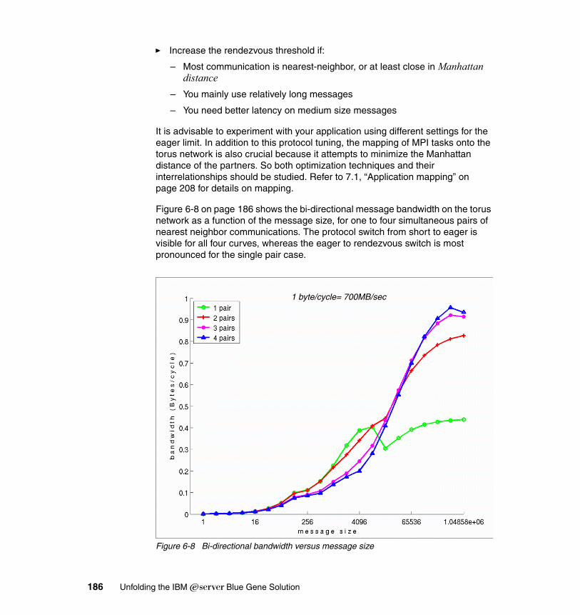
� Increase the rendezvous threshold if:

– Most communication is nearest-neighbor, or at least close in Manhattan distance

– You mainly use relatively long messages

– You need better latency on medium size messages

It is advisable to experiment with your application using different settings for the eager limit. In addition to this protocol tuning, the mapping of MPI tasks onto the torus network is also crucial because it attempts to minimize the Manhattan distance of the partners. So both optimization techniques and their interrelationships should be studied. Refer to 7.1, “Application mapping” on page 208 for details on mapping.

Figure 6-8 on page 186 shows the bi-directional message bandwidth on the torus network as a function of the message size, for one to four simultaneous pairs of nearest neighbor communications. The protocol switch from short to eager is visible for all four curves, whereas the eager to rendezvous switch is most pronounced for the single pair case.

Figure 6-8 Bi-directional bandwidth versus message size

1 byte/cycle= 700MB/sec


The raw hardware bandwidth of each link on the torus network is 2 bit or 0.25 byte per cycle per direction, which is 175 MB/sec per link per direction on the 700 MHz nodes. So the peak bi-directional bandwidth for a single pair is limited by the torus network hardware to 0.5 byte/cycle, and for two pairs to 1 byte/cycle. For three and more pairs of simultaneous communications, the bandwidth does not increase over the two-pair case: it is now limited by the node’s ability to drive the communication rather than by the network bandwidth.

Some more considerations regarding point-to-point performance:

� Don’t attempt to overlap communication and computation.

While this may work on other architectures, trying to overlap communication and computation is generally a bad idea on Blue Gene/L. You should instead organize your program in such a way that computation phases alternate with communication phases, and of course try to keep your program’s tasks as synchronized as possible.

� Avoid load imbalance.

This is important for all parallel systems, but when scaling to the high numbers of tasks that are possible on Blue Gene/L, it is especially important to pay close attention to load balancing.

� Avoid buffered and synchronous sends; post receives in advance.

The MPI standard defines several specialized communication modes in addition to the standard send function, MPI_Send(). The buffered send function, MPI_Bsend() should be avoided because forcing the MPI library to perform additional memory copies will slow down the application, and you may also run short of memory so additional buffering may not be possible at all. Using the synchronous send function MPI_Ssend() is discouraged because it is a non-local operation that will incur an increased latency compared to the standard send. On the other hand, the ready send operation MPI_Rsend() may be used. A ready send is only allowed if a matching receive has already been posted. This helps communication performance, as does posting receives in advance of any send operation, because the receiver will be expecting the incoming messages. Unexpected messages need to be buffered, whereas expected messages can be transferred immediately into the user’s receive buffer.

� Avoid vector data and non-contiguous data types.

While the MPI derived data types can elegantly describe the layout of complex data structures, using these data types is generally detrimental to performance. Many MPI implementations will pack (that is, memory-copy) such data objects before sending them, which is contrary to the original purpose of MPI-derived data types (namely to avoid such memory copies). In addition, the BG/L MPI implementation makes use of the chips’ special


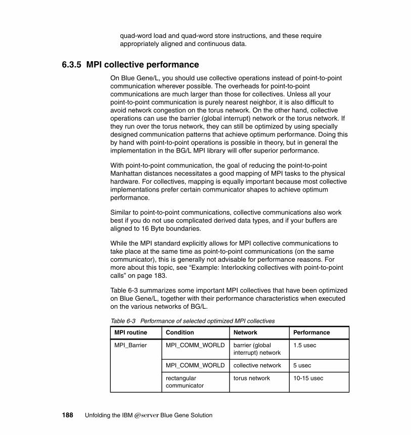
quad-word load and quad-word store instructions, and these require appropriately aligned and continuous data.

6.3.5 MPI collective performanceOn Blue Gene/L, you should use collective operations instead of point-to-point communication wherever possible. The overheads for point-to-point communications are much larger than those for collectives. Unless all your point-to-point communication is purely nearest neighbor, it is also difficult to avoid network congestion on the torus network. On the other hand, collective operations can use the barrier (global interrupt) network or the torus network. If they run over the torus network, they can still be optimized by using specially designed communication patterns that achieve optimum performance. Doing this by hand with point-to-point operations is possible in theory, but in general the implementation in the BG/L MPI library will offer superior performance.

With point-to-point communication, the goal of reducing the point-to-point Manhattan distances necessitates a good mapping of MPI tasks to the physical hardware. For collectives, mapping is equally important because most collective implementations prefer certain communicator shapes to achieve optimum performance.

Similar to point-to-point communications, collective communications also work best if you do not use complicated derived data types, and if your buffers are aligned to 16 Byte boundaries.

While the MPI standard explicitly allows for MPI collective communications to take place at the same time as point-to-point communications (on the same communicator), this is generally not advisable for performance reasons. For more about this topic, see “Example: Interlocking collectives with point-to-point calls” on page 183.

Table 6-3 summarizes some important MPI collectives that have been optimized on Blue Gene/L, together with their performance characteristics when executed on the various networks of BG/L.

Table 6-3 Performance of selected optimized MPI collectives

MPI routine Condition Network Performance

MPI_Barrier MPI_COMM_WORLD barrier (global interrupt) network

1.5 usec

MPI_COMM_WORLD collective network 5 usec

rectangular communicator

torus network 10-15 usec


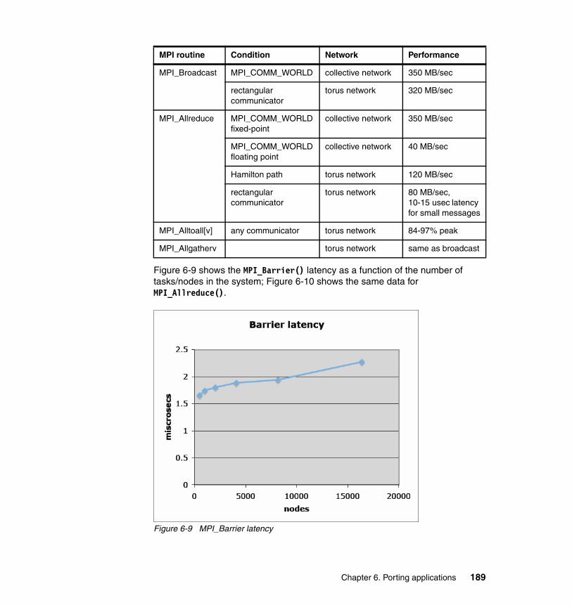
Figure 6-9 shows the MPI_Barrier() latency as a function of the number of tasks/nodes in the system; Figure 6-10 shows the same data for MPI_Allreduce().

Figure 6-9 MPI_Barrier latency

MPI_Broadcast MPI_COMM_WORLD collective network 350 MB/sec


torus network 320 MB/sec

MPI_Allreduce MPI_COMM_WORLDfixed-point

collective network 350 MB/sec

MPI_COMM_WORLDfloating point

collective network 40 MB/sec

Hamilton path torus network 120 MB/sec


torus network 80 MB/sec,10-15 usec latency for small messages

MPI_Alltoall[v] any communicator torus network 84-97% peak

MPI_Allgatherv torus network same as broadcast

MPI routine Condition Network Performance


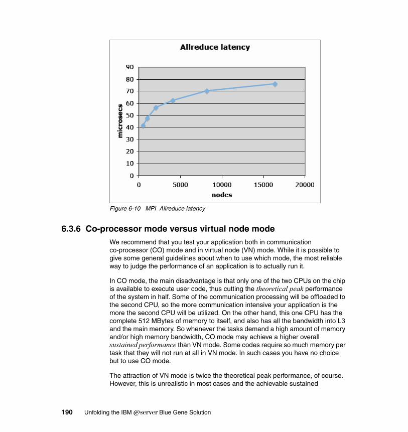
Figure 6-10 MPI_Allreduce latency

6.3.6 Co-processor mode versus virtual node modeWe recommend that you test your application both in communication co-processor (CO) mode and in virtual node (VN) mode. While it is possible to give some general guidelines about when to use which mode, the most reliable way to judge the performance of an application is to actually run it.

In CO mode, the main disadvantage is that only one of the two CPUs on the chip is available to execute user code, thus cutting the theoretical peak performance of the system in half. Some of the communication processing will be offloaded to the second CPU, so the more communication intensive your application is the more the second CPU will be utilized. On the other hand, this one CPU has the complete 512 MBytes of memory to itself, and also has all the bandwidth into L3 and the main memory. So whenever the tasks demand a high amount of memory and/or high memory bandwidth, CO mode may achieve a higher overall sustained performance than VN mode. Some codes require so much memory per task that they will not run at all in VN mode. In such cases you have no choice but to use CO mode.

The attraction of VN mode is twice the theoretical peak performance, of course. However, this is unrealistic in most cases and the achievable sustained


performance is very much dependent on the application. Compared to CO mode, in VN mode the cache, memory, and network bandwidths are halved, as are the cache and memory sizes available to the application. For applications which are not very demanding with respect to these resources. VN mode can nevertheless result in significant performance improvements. Chapter 8 contains some examples where VN mode worked very well, sometimes surprisingly well. So it is always worth investigating the performance of your application in both modes.

6.4 I/O operationsThe method used for reading data into the compute nodes and writing data out from the compute nodes is completely different on Blue Gene/L than on other systems which readers may be familiar with.

It may be possible to run code on Blue Gene/L by following the rules for porting code from other platforms, enabling the code to compile and run, but the actual performance of the code may be limited by the way the code is performing I/O.

Understanding the I/O implementation on Blue Gene/L is a pre-requisite to understanding how to restructure code to circumvent I/O bottlenecks.

On the other hand, anyone wanting to port and run codes which are not limited by I/O performance need not understand the Blue Gene/L I/O architecture.

This section is an overview of how I/O operations are handled by Blue Gene/L, and also includes some discussion of how it might be possible to make code enhancements to improve aggregate I/O performance.

6.4.1 How the I/O worksEach Blue Gene/L node has five network connections:

1. Gigabit Ethernet2. JTAG3. Torus4. Collective (sometimes called tree)5. Global Interrupt (sometimes called barrier)

There is provision for all five network connections on every Blue Gene/L chip, but whereas the I/O nodes have a Gigabit Ethernet interface, the compute nodes do not, meaning the network connection from the chip does not connect to anything.

Conversely, the I/O nodes have no connections to the torus network, which is used for the majority of MPI communication between compute nodes.


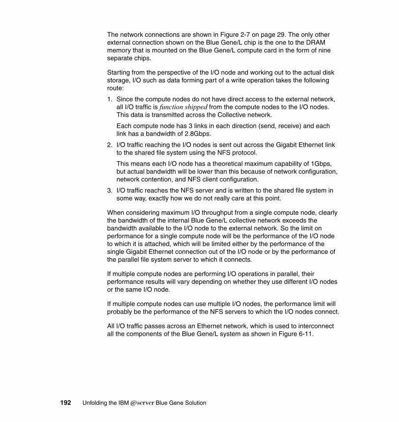
The network connections are shown in Figure 2-7 on page 29. The only other external connection shown on the Blue Gene/L chip is the one to the DRAM memory that is mounted on the Blue Gene/L compute card in the form of nine separate chips.

Starting from the perspective of the I/O node and working out to the actual disk storage, I/O such as data forming part of a write operation takes the following route:

1. Since the compute nodes do not have direct access to the external network, all I/O traffic is function shipped from the compute nodes to the I/O nodes. This data is transmitted across the Collective network.

Each compute node has 3 links in each direction (send, receive) and each link has a bandwidth of 2.8Gbps.

2. I/O traffic reaching the I/O nodes is sent out across the Gigabit Ethernet link to the shared file system using the NFS protocol.

This means each I/O node has a theoretical maximum capability of 1Gbps, but actual bandwidth will be lower than this because of network configuration, network contention, and NFS client configuration.

3. I/O traffic reaches the NFS server and is written to the shared file system in some way, exactly how we do not really care at this point.

When considering maximum I/O throughput from a single compute node, clearly the bandwidth of the internal Blue Gene/L collective network exceeds the bandwidth available to the I/O node to the external network. So the limit on performance for a single compute node will be the performance of the I/O node to which it is attached, which will be limited either by the performance of the single Gigabit Ethernet connection out of the I/O node or by the performance of the parallel file system server to which it connects.

If multiple compute nodes are performing I/O operations in parallel, their performance results will vary depending on whether they use different I/O nodes or the same I/O node.

If multiple compute nodes can use multiple I/O nodes, the performance limit will probably be the performance of the NFS servers to which the I/O nodes connect.

All I/O traffic passes across an Ethernet network, which is used to interconnect all the components of the Blue Gene/L system as shown in Figure 6-11.


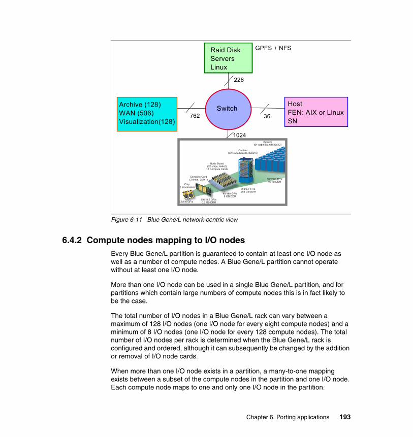
Figure 6-11 Blue Gene/L network-centric view

6.4.2 Compute nodes mapping to I/O nodesEvery Blue Gene/L partition is guaranteed to contain at least one I/O node as well as a number of compute nodes. A Blue Gene/L partition cannot operate without at least one I/O node.

More than one I/O node can be used in a single Blue Gene/L partition, and for partitions which contain large numbers of compute nodes this is in fact likely to be the case.

The total number of I/O nodes in a Blue Gene/L rack can vary between a maximum of 128 I/O nodes (one I/O node for every eight compute nodes) and a minimum of 8 I/O nodes (one I/O node for every 128 compute nodes). The total number of I/O nodes per rack is determined when the Blue Gene/L rack is configured and ordered, although it can subsequently be changed by the addition or removal of I/O node cards.

When more than one I/O node exists in a partition, a many-to-one mapping exists between a subset of the compute nodes in the partition and one I/O node. Each compute node maps to one and only one I/O node in the partition.

Raid DiskServersLinux

Archive (128)WAN (506)Visualization(128)

SwitchHostFEN: AIX or LinuxSN

762 36

226

1024

GPFS + NFS

Chip(2 processors)

Compute Card(2 chips, 2x1x1)

Node Board(32 chips, 4x4x2)

16 Compute Cards

System(64 cabinets, 64x32x32)

Cabinet(32 Node boards, 8x8x16)

2.8/5.6 GF/s4 MB

5.6/11.2 GF/s0.5 GB DDR

90/180 GF/s8 GB DDR

2.9/5.7 TF/s256 GB DDR

180/360 TF/s16 TB DDR


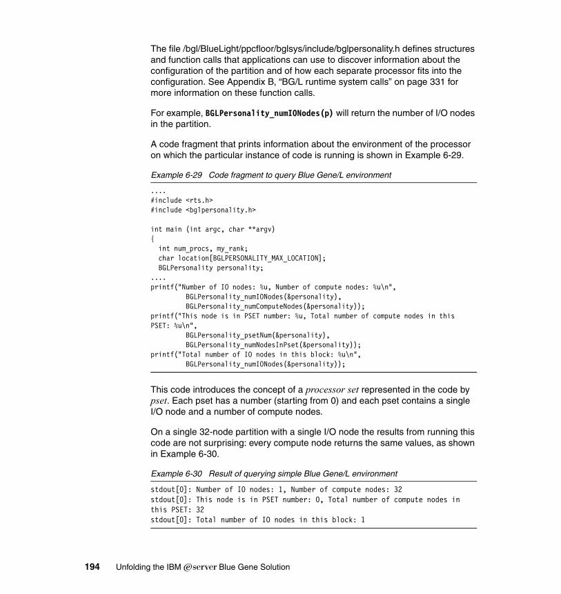
The file /bgl/BlueLight/ppcfloor/bglsys/include/bglpersonality.h defines structures and function calls that applications can use to discover information about the configuration of the partition and of how each separate processor fits into the configuration. See Appendix B, “BG/L runtime system calls” on page 331 for more information on these function calls.

For example, BGLPersonality_numIONodes(p) will return the number of I/O nodes in the partition.

A code fragment that prints information about the environment of the processor on which the particular instance of code is running is shown in Example 6-29.

Example 6-29 Code fragment to query Blue Gene/L environment

....#include <rts.h>#include <bglpersonality.h>

int main (int argc, char **argv){ int num_procs, my_rank; char location[BGLPERSONALITY_MAX_LOCATION]; BGLPersonality personality;....printf("Number of IO nodes: %u, Number of compute nodes: %u\n", BGLPersonality_numIONodes(&personality), BGLPersonality_numComputeNodes(&personality));printf("This node is in PSET number: %u, Total number of compute nodes in this PSET: %u\n", BGLPersonality_psetNum(&personality), BGLPersonality_numNodesInPset(&personality));printf("Total number of IO nodes in this block: %u\n", BGLPersonality_numIONodes(&personality));

This code introduces the concept of a processor set represented in the code by pset. Each pset has a number (starting from 0) and each pset contains a single I/O node and a number of compute nodes.

On a single 32-node partition with a single I/O node the results from running this code are not surprising: every compute node returns the same values, as shown in Example 6-30.

Example 6-30 Result of querying simple Blue Gene/L environment

stdout[0]: Number of IO nodes: 1, Number of compute nodes: 32stdout[0]: This node is in PSET number: 0, Total number of compute nodes in this PSET: 32stdout[0]: Total number of IO nodes in this block: 1


In all cases, each compute node is a member of one pset, which can be identified by a number, and all compute nodes in the same pset perform their I/O through the same I/O node. Also, every Blue Gene/L partition contains a number of psets equivalent to the number of I/O nodes in the partition.

6.4.3 Do not use one file per I/O nodeTo increase the aggregate I/O it is a good idea to make multiple compute nodes initiate I/O operations, but you have to make sure that they each don’t perform these operations on separate files. Having 65,536 compute nodes driving I/O separately is probably OK, but not if they cause 65,536 distinct files on the file system to be opened in parallel. This may generate a lot of file system metadata activity which may result in a very slow file system.

6.4.4 Do not use one task doing all I/OA common model for parallel codes is one in which all I/O is performed by a single node even though the computation work is shared between the nodes. If an application which conforms to this model is ported to Blue Gene/L, the I/O performance will be limited by the performance of a single compute node, which means that it will also be limited by the performance of a single I/O node.

The first step to improve total I/O performance of a Blue Gene/L cluster is to share I/O operations across multiple I/O nodes by causing the operations to be initiated from multiple compute nodes which are members of different psets.

If the I/O operations can be spread evenly across all the compute nodes, this will probably lead to a balanced load across all the I/O nodes.

However, if it is possible to maximize aggregate I/O performance by having all the compute nodes perform I/O operations, it is probably unwise to have each compute node performing I/O on a separate file in the file system. This would lead to usability problems with large jobs (how could we make use of 65,536 separate small output files, for example), and would also lead to poor performance by making the I/O servers perform operations on large numbers of files in parallel.

Note: In most Blue Gene/L implementations, spreading the I/O load across all the compute nodes will indeed lead to a balanced load across all the I/O nodes. It is unlikely, but possible, that the ratio of compute nodes to I/O nodes is not constant across a single partition, if different Blue Gene/L midplanes have been implemented with different I/O node ratios. Hence the use of the word probably in the previous paragraph.


If the I/O operations are spread across a subset of the compute nodes, use care to ensure that the compute nodes chosen map to different I/O nodes. This may require explicit programming support.

6.5 DebuggingDebugging applications on Blue Gene/L is different from debugging on stand-alone machines or clusters because the application runs on the compute nodes which only have a microkernel, whereas the application developer is logged in to the front-end node.

Currently, very little system-level information about the compute nodes’ status is available. Running commands like ps or top to find out the CPU and memory usage of the compute nodes is not possible on Blue Gene/L. A job shown as running in the MMCS may be performing useful work, or may be deadlocked and not perform any work at all.

Therefore, all debugging must be done explicitly in the application program. In this section we discuss several ways to do this.

6.5.1 Debugging by printf() or PRINTEveryone knows the time-proven debugging technique of inserting printf() or PRINT lines into the program to print out progress information or values of variables. This does work on Blue Gene/L too, of course. All standard output and standard errors will be written to the job’s <block-id>-<job-id>.stdout and <block-id>-<job-id>.stderr files.

If you are debugging a parallel application but are only interested in output from a single task, it is useful to limit the display of stdout/stderr to just one task. This can be easily done by filtering the output files like this:

grep "stdout\[0\]" R00-M0-N0_1-7255.stdout

This will show only the output from MPI task 0.

6.5.2 Instrumenting function entry and exitThe XL compilers have an option which allows calling user-supplied functions on entry and exit of all functions/subprograms in the application. We have found this facility very useful for many situations where there are no other tools available to dig into a problem. The strength of this approach comes from the fact that no modifications of the original source files are necessary.


To instrument your program’s function calls, perform the following steps:

1. Write the instrumentation code.

The user has to provide two functions, which will be called by the runtime system, with the following arguments:

__function_trace_enter ("routineName", "filename", lineNo)__function_trace_exit ("routineName", "filename", lineNo)

Note that the function names begin with two underscores. When compiling these routines, you should not use the compiler option to instrument function calls or you will end up with an infinite call chain.

2. Compile the application with -qdebug=function_trace.

3. Link the application with your instrumentation code.

For small test cases you may just use the object file that contains the instrumentation code. For more general routines that can be useful to many users, it is a good idea to put them into a library and place the library in a directory that is in the library search path.

4. Run the application.

Here is an example that just prints the information that the compiler provides to the instrumentation calls. First we create a source file with the code for the two functions (Example 6-31).

Example 6-31 Sample source file for instrumentation calls

$cat func_trace.c#include <stdio.h>__func_trace_enter(char *routine_name, char *file_name, int line_number){ printf(“__func_trace_enter: routine %s in file %s, line %i\n”, routine_name, file_name, line_number);}__func_trace_exit(char *routine_name, char *file_name, int line_number){ printf(“__func_trace_exit: routine %s in file %s, line %i\n”, routine_name, file_name, line_number);}

Next we compile the source file into an object file (-g is not necessary for this functionality), put the object file into a library, and place that library in our /bgl/local/lib/ directory, which is in our default library search path:

$ blrts_xlc -g -c func_trace.c$ ar rv libfunc_trace.a func_trace.o$ chmod a+r libfunc_trace.a$ cp -p libfunc_trace.a /bgl/local/lib/


Now the user application is compiled with the -qdebug=function_trace compiler option, which enables the instrumentation (again, -g is not necessary for the instrumentation, but is useful for traditional debugging), and it is finally linked with the instrumentation code, as in Example 6-32.

Example 6-32 Using the -qdebug=function_trace option

$ blrts_xlf90 -g -c -qdebug=function_trace example.f

# link using the object file:$ blrts_xlf -g example.o func_trace.o -o example.rts# alternatively, link to the library:$ blrts_xlf -g example.o -o example.rts -L /bgl/local/lib -l func_trace

If you execute example.rts on the compute nodes, each function entry and exit will print a line giving the name of the routine, together with the file name and line number.

6.5.3 Using the GNU debuggerThe GNU debugger gdb can be used to debug applications running on the Blue Gene/L compute nodes. It has a built-in mechanism to connect to applications running on other machines, by using a gdbserver program on the remote side.

On Blue Gene/L, a special version of the gdbserver has been implemented. It is named gdbserver.440 and is located in /bgl/BlueLight/ppcfloor/dist/sbin/. It runs on the I/O nodes, which in turn control the compute nodes attached to them. The gdbserver.440 process allows gdb connections via TCP/IP by opening one socket for each compute node in the I/O node’s pset, starting at port 17300 for the first MPI task in the pset.

In the following discussion, we refer to the gdbserver.440 server simply as the gdbserver.

The Blue Gene/L version of gdb is available on the front-end nodes at the following location:

/bgl/BlueLight/ppcfloor/linux-gnu/bin/powerpc-bgl-linux-gnu-gdb

Attention: We have seen cases where the port numbers reported (for example, by the MMCS dump_proctable command) were off by one, so the first reported port was 17299 not 17300. Still, the first port actually used was 17300 and not 17299. This is a bug that will eventually be fixed.


When debugging Blue Gene/L applications, make sure that you use this version of gdb and not the one at /usr/bin/gdb, which is the standard version for Linux on POWER that comes with the SLES distribution.

Compiling your executableSimilar to debugging on other platforms, you should compile your application using the -g compiler option. If possible, the libraries you are using should also be compiled with the -g option.

The XL compilers support the use of -g in conjunction with -O, but of course the higher your optimizing level the more difficult will it be to associate instructions in the executable with statements in the original source file. In general, using -O2 gives good results.

Starting gdbserver through the MMCS consoleYou can start gdbserver through commands in the MMCS console. However, this method only allows you to attach to an already running job. You submit the job as usual, and when it runs you can tell MMCS to start gdbserver for this job. The handshaking that is required to start a job under gdbserver from the beginning is only available through the mpirun command. This is explained in the next section.

Here is a complete example of the steps that are needed to start gdbserver through the MMCS console:

1. Start the mmcs_db_console and allocate a block:

$ mmcs_db_consolemmcs$ allocate R00-M0-N0_1OK

2. Among the properties of the block are the path to the gdbserver executable and any options that may be passed to it when it’s started. To check what is set for the block you have allocated, use the MMCS list bglblock command (Example 6-33).

Example 6-33 MMCS list bglblock command

mmcs$ list bglblock R00-M0-N0_1==> DBBlock record_blockid = R00-M0-N0_1..._debuggerimg = none_debuggerparms = 20202020202020202020202020202020202020202020202020202020202020202020202020202020202020202020202020202020202020202020202020202020 (truncated)_debuggerparmsize = 0


...

In this case the path to the gdbserver is not stored in the _debuggerimg field of the block.

3. To be able to start gdbserver, you need to add its full path. Do this using the MMCS setdebuginfo command (Example 6-34).

Example 6-34 MMCS setdebuginfo command

mmcs$ help setdebuginfosetdebuginfo <blockid> <debugger> [ args ]Set the debugger image, and optional debugger arguments for a blockmmcs$ setdebuginfo R00-M0-N0_1 /bgl/BlueLight/ppcfloor/dist/sbin/gdbserver.440debug info set with success for block R00-M0-N0_1

4. If you now re-run the MMCS list bglblock command, you should see the full path in the _debuggerimg field. No arguments to gdbserver are necessary. The settings entered by setdebuginfo are persistent across block allocations, so you only need to set them once (for each block, of course).

5. After you have verified that the block has a valid _debuggerimg entry, you can submit your job. You need to remember the jobId, which you pass to the MMCS debugjob command:

mmcs$ submitjob R00-M0-N0_1 /bgl/hennecke/debug-case.rts /bgl/henneckeOKjobId=9437

6. When the job has started running, and is therefore in job state R, you can use the MMCS debugjob command to start gdbserver:

mmcs$ debugjob 9437Job 9437 will have debugger started

If you run debugjob before the job is running, you will get an error message similar to the following:

mmcs$ debugjob 9944change of state for job 9944 failed.

Should this happen, just wait until the job runs and then re-issue the debugjob command.

7. To attach your gdb session on the front-end node to a specific MPI task, you need to find out which I/O node controls the compute node that runs this MPI task, and the port number that gdbserver has opened for it. You can get this information through the MMCS dump_proctable command. For each MPI task it will list the <ip-addr>:<port> combination that you can use to attach gdb to that MPI task (Example 6-35).


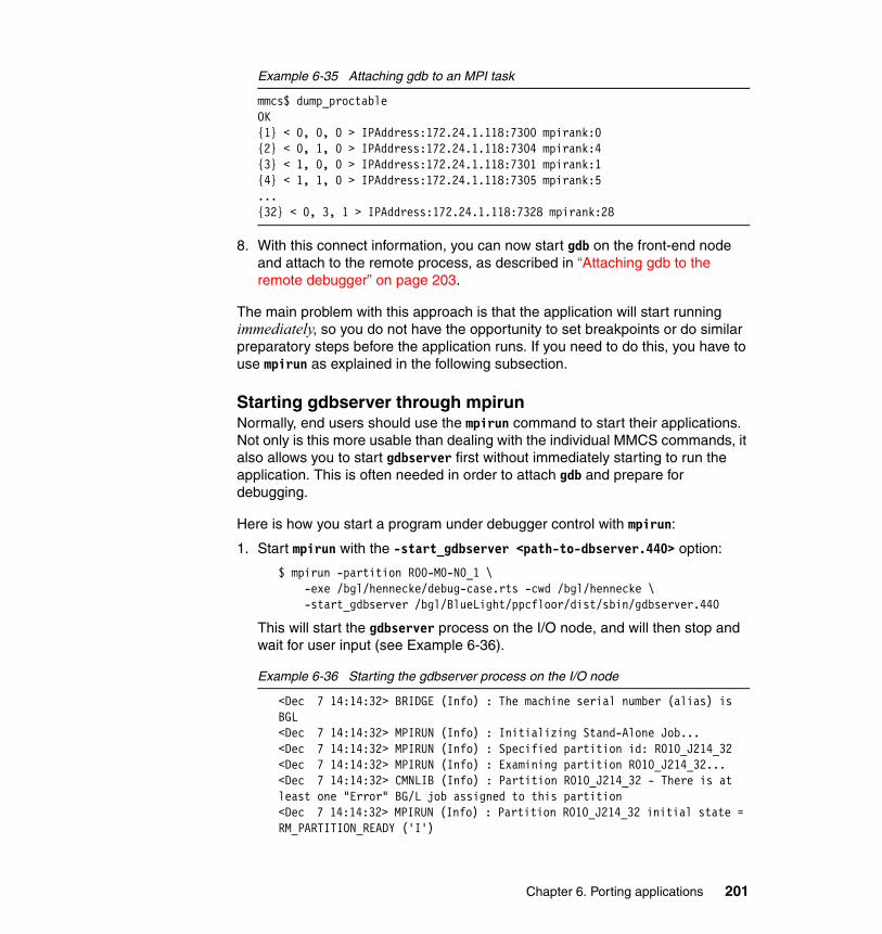
Example 6-35 Attaching gdb to an MPI task

mmcs$ dump_proctableOK{1} < 0, 0, 0 > IPAddress:172.24.1.118:7300 mpirank:0{2} < 0, 1, 0 > IPAddress:172.24.1.118:7304 mpirank:4{3} < 1, 0, 0 > IPAddress:172.24.1.118:7301 mpirank:1{4} < 1, 1, 0 > IPAddress:172.24.1.118:7305 mpirank:5...{32} < 0, 3, 1 > IPAddress:172.24.1.118:7328 mpirank:28

8. With this connect information, you can now start gdb on the front-end node and attach to the remote process, as described in “Attaching gdb to the remote debugger” on page 203.

The main problem with this approach is that the application will start running immediately, so you do not have the opportunity to set breakpoints or do similar preparatory steps before the application runs. If you need to do this, you have to use mpirun as explained in the following subsection.

Starting gdbserver through mpirunNormally, end users should use the mpirun command to start their applications. Not only is this more usable than dealing with the individual MMCS commands, it also allows you to start gdbserver first without immediately starting to run the application. This is often needed in order to attach gdb and prepare for debugging.

Here is how you start a program under debugger control with mpirun:

1. Start mpirun with the -start_gdbserver <path-to-dbserver.440> option:

$ mpirun -partition R00-M0-N0_1 \-exe /bgl/hennecke/debug-case.rts -cwd /bgl/hennecke \-start_gdbserver /bgl/BlueLight/ppcfloor/dist/sbin/gdbserver.440

This will start the gdbserver process on the I/O node, and will then stop and wait for user input (see Example 6-36).

Example 6-36 Starting the gdbserver process on the I/O node

<Dec 7 14:14:32> BRIDGE (Info) : The machine serial number (alias) is BGL<Dec 7 14:14:32> MPIRUN (Info) : Initializing Stand-Alone Job...<Dec 7 14:14:32> MPIRUN (Info) : Specified partition id: R010_J214_32<Dec 7 14:14:32> MPIRUN (Info) : Examining partition R010_J214_32...<Dec 7 14:14:32> CMNLIB (Info) : Partition R010_J214_32 - There is at least one "Error" BG/L job assigned to this partition<Dec 7 14:14:32> MPIRUN (Info) : Partition R010_J214_32 initial state = RM_PARTITION_READY ('I')


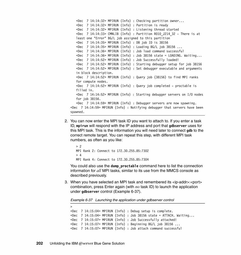
<Dec 7 14:14:32> MPIRUN (Info) : Checking partition owner...<Dec 7 14:14:32> MPIRUN (Info) : Partition is ready<Dec 7 14:14:32> MPIRUN (Info) : Listening thread started<Dec 7 14:14:33> CMNLIB (Info) : Partition R010_J214_32 - There is at least one "Error" BG/L job assigned to this partition<Dec 7 14:14:35> MPIRUN (Info) : DB job ID is 38156<Dec 7 14:14:35> MPIRUN (Info) : Loading BG/L job 38156 ...<Dec 7 14:14:36> MPIRUN (Info) : Job load command successful<Dec 7 14:14:36> MPIRUN (Info) : Job 38156 state = LOADING. Waiting...<Dec 7 14:14:52> MPIRUN (Info) : Job Successfully loaded!<Dec 7 14:14:52> MPIRUN (Info) : Starting debugger setup for job 38156<Dec 7 14:14:52> MPIRUN (Info) : Set debugger executable and arguments in block description.<Dec 7 14:14:52> MPIRUN (Info) : Query job (38156) to find MPI ranks for compute nodes.<Dec 7 14:14:52> MPIRUN (Info) : Query job completed - proctable is filled in.<Dec 7 14:14:52> MPIRUN (Info) : Starting debugger servers on I/O nodes for job 38156.<Dec 7 14:14:59> MPIRUN (Info) : Debugger servers are now spawning.

<Dec 7 14:14:59> MPIRUN (Info) : Notifying debugger that servers have been spawned.

2. You can now enter the MPI task ID you want to attach to. If you enter a task ID, mpirun will respond with the IP address and port that gdbserver uses for this MPI task. This is the information you will need later to connect gdb to the correct remote target. You can repeat this step, with different MPI task numbers, as often as you like:

> 2MPI Rank 2: Connect to 172.30.255.85:7302> 4MPI Rank 4: Connect to 172.30.255.85:7304

You could also use the dump_proctable command here to list the connection information for all MPI tasks, similar to its use from the MMCS console as described previously.

3. When you have selected an MPI task and remembered its <ip-addr>:<port> combination, press Enter again (with no task ID) to launch the application under gdbserver control (Example 6-37).

Example 6-37 Launching the application under gdbserver control

> <Dec 7 14:15:04> MPIRUN (Info) : Debug setup is complete.<Dec 7 14:15:04> MPIRUN (Info) : Job 38156 state = ATTACH. Waiting...<Dec 7 14:15:07> MPIRUN (Info) : Job Successfully attached!<Dec 7 14:15:07> MPIRUN (Info) : Beginning BG/L job 38156 ...<Dec 7 14:15:07> MPIRUN (Info) : Job attach command successful


<Dec 7 14:15:07> MPIRUN (Info) : Waiting for job to terminate...

4. If you need to prepare the application before it starts running, use gdb from another login session and attach to gdbserver before pressing enter in mpirun. Do all your preparatory work (like defining breakpoints), and when you are ready to run, press Enter within the waiting mpirun session to start the application.

It is also possible to attach to an already running program that has been started through mpirun but without specifying -start_gdbserver. There are two ways to do this:

1. Use MMCS and its debugjob command, as described previously.

2. Connect gdb to mpirun (instead of the application), and set some special runtime variables that tell mpirun that a debug session should be started.

$ powerpc-bgl-linux-gnu-gdb example.rtsGNU gdb 5.3Copyright 2002 Free Software Foundation, Inc....

(gdb) set MPIR_executable_path = "/bgl/BlueLight/ppcfloor/linux-gnu/bin/powerpc-linux-gnu-gdb"

(gdb) set MPIR_server_arguments = "\0\0"(gdb) set MPIR_being_debugged = 1(gdb) c

To save some typing, the commands to set these variables can be stored in a gdb command file, and parsed by using gdb -x. This is described in the next section.

Attaching gdb to the remote debuggerOnce gdbserver has been launched on the I/O nodes, you can start gdb on the front-end node and connect to gdbserver. As usual, the name of the executable to be debugged should be specified as an argument to gdb.

$ powerpc-bgl-linux-gnu-gdb example.rtsGNU gdb 5.3Copyright 2002 Free Software Foundation, Inc....(gdb)

If you get to the gdb prompt, use the target remote command of gdb to connect to gdbserver, using the IP address and port number for the MPI task you want to attach to. After this connect, you can use gdb as on any other platform:

(gdb) target remote 172.24.1.118:7300Remote debugging using 172.24.1.118:7300...


(gdb)... normal gdb usage from here ...(gdb) detachEnding remote debugging.(gdb) quit

Note that if you quit gdb without detach, gdb will kill the application.

If you are running multiple debug sessions which always attach to the same MPI task in the same MMCS block, it is handy to put the target command into a gdb command file and invoke that via the gdb -x option, rather than retyping it every time:

$ cat ./gdbrctarget remote 172.24.1.118:7300

$ powerpc-bgl-linux-gnu-gdb -x ./gdbrc example.rts... normal gdb usage ...(gdb) detach(gdb) quit

If you name this file .gdbinit in your current working directory, it will automatically be picked up by gdb without the need for a -x option.

6.5.4 TotalViewAt the time of writing, the TotalView debugger by Etnus was announced, but not yet available on Blue Gene/L.

Restriction:

The gdb run command does not work. Trying to restart the application from the beginning using gdb consistently crashed the application when we tried it:

(gdb) runThe program being debugged has been started already.Start it from the beginning? (y or n) y

Starting program: /auto/export-bglsim/hennecke/debug-case.rtsÿÿáProgram received signal SIGSEGV, Segmentation fault.0x00168fbc in chunk_free (ar_ptr=0x1d2cd0, p=0xffffe0f8) at malloc.c:32273227 malloc.c: No such file or directory. in malloc.c(gdb)


6.5.5 Debugging parallel programsWhen available, TotalView will be the debugger of choice to debug parallel applications.

It is possible to have multiple gdb sessions attached to multiple MPI tasks, but this is not very usable.

6.5.6 Tracking your memory usageRunning out of memory may cause a SIGSEGV or not, depending on the circumstances. It is useful to know how much memory you actually use.

Calling sbrk(0) gives you the current limit of the data area.

You can use the -qdebug=function_trace compiler option to instrument function entry and exit to monitor this. Check with the IBM development team for more information.

A quick test shows that (with no significant program text) you can get to ca. 508 MiB on a CN before running out of memory.

This is all applicable to serial programs too. For parallel programs it is especially important that you check all arrays whose size depends on the number of tasks (for example, MPI_COMM_SIZE). Try to eliminate that dependency, or distribute the array across the tasks. Otherwise, this will cause memory overrun if the number of tasks becomes higher and higher. Many data structures have been designed with O(10) to O(100) tasks in mind, and memory consumption of replicated arrays will explode for O(1000) or O(10000) tasks.

6.5.7 Core files and addr2lineCompile your program with -g as usual. If you get a core dump, the core file actually is a plain text file that you can view with more or a text editor.

You can the use the Linux addr2line command on the front-end node, give it the address found in the core file and the -g executable, and it will point you to the source line where the problem occurred.

Tip: To save program text space on the compute node, save a copy of your executable compiled with -g for later use with addr2line. Make another copy of the executable and strip it. Use that stripped executable to run on the compute node. If it core dumps and you want to use addr2line, just give addr2line the unstripped executable.


Of course, this will not help if the exception was in a library external to your program that has not been compiled with the -g flag. In that case, you can look at the calling stack and find where it left your own code, at least.


Chapter 7. Massively parallel tuning

This chapter discusses various ways to make your application exploit the large number of processors (up to 131072 CPUs) available on a BG/L system.

It also presents hints that may help you to determine, in certain situations, why your application does not scale as expected.

7


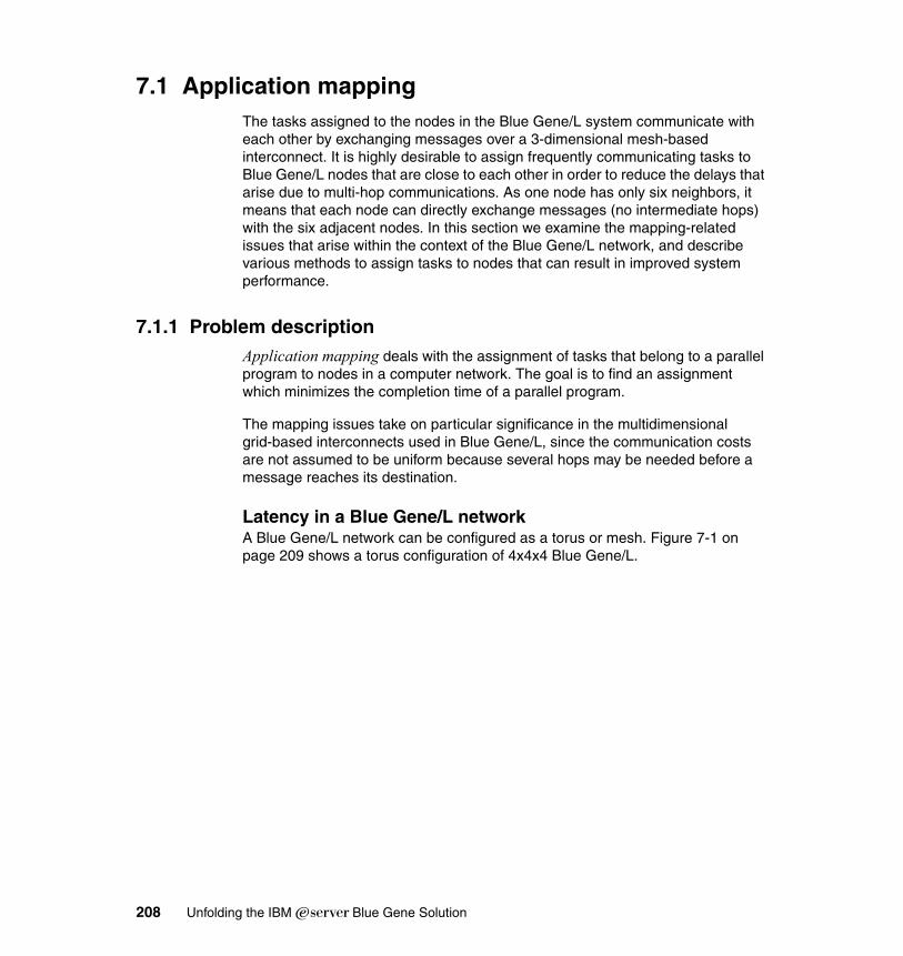
7.1 Application mappingThe tasks assigned to the nodes in the Blue Gene/L system communicate with each other by exchanging messages over a 3-dimensional mesh-based interconnect. It is highly desirable to assign frequently communicating tasks to Blue Gene/L nodes that are close to each other in order to reduce the delays that arise due to multi-hop communications. As one node has only six neighbors, it means that each node can directly exchange messages (no intermediate hops) with the six adjacent nodes. In this section we examine the mapping-related issues that arise within the context of the Blue Gene/L network, and describe various methods to assign tasks to nodes that can result in improved system performance.

7.1.1 Problem descriptionApplication mapping deals with the assignment of tasks that belong to a parallel program to nodes in a computer network. The goal is to find an assignment which minimizes the completion time of a parallel program.

The mapping issues take on particular significance in the multidimensional grid-based interconnects used in Blue Gene/L, since the communication costs are not assumed to be uniform because several hops may be needed before a message reaches its destination.

Latency in a Blue Gene/L networkA Blue Gene/L network can be configured as a torus or mesh. Figure 7-1 on page 209 shows a torus configuration of 4x4x4 Blue Gene/L.


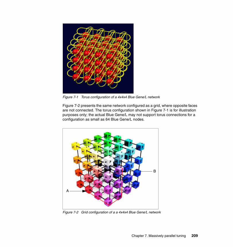
Figure 7-1 Torus configuration of a 4x4x4 Blue Gene/L network

Figure 7-2 presents the same network configured as a grid, where opposite faces are not connected. The torus configuration shown in Figure 7-1 is for illustration purposes only; the actual Blue Gene/L may not support torus connections for a configuration as small as 64 Blue Gene/L nodes.

Figure 7-2 Grid configuration of a a 4x4x4 Blue Gene/L network

B

A

Chapter 7. Massively parallel tuning 209

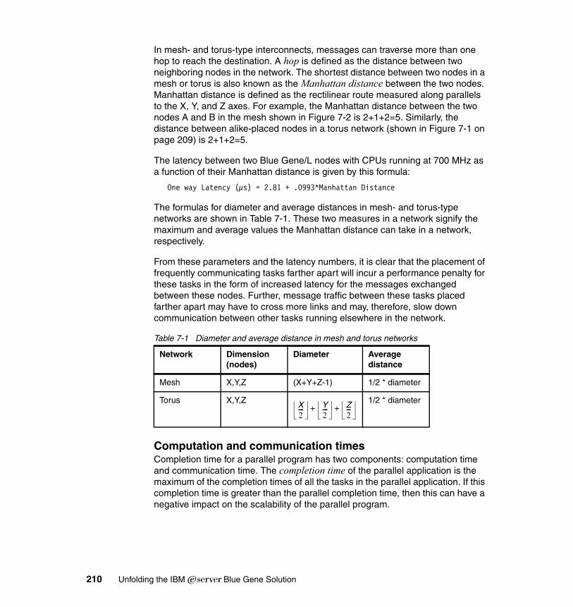
In mesh- and torus-type interconnects, messages can traverse more than one hop to reach the destination. A hop is defined as the distance between two neighboring nodes in the network. The shortest distance between two nodes in a mesh or torus is also known as the Manhattan distance between the two nodes. Manhattan distance is defined as the rectilinear route measured along parallels to the X, Y, and Z axes. For example, the Manhattan distance between the two nodes A and B in the mesh shown in Figure 7-2 is 2+1+2=5. Similarly, the distance between alike-placed nodes in a torus network (shown in Figure 7-1 on page 209) is 2+1+2=5.

The latency between two Blue Gene/L nodes with CPUs running at 700 MHz as a function of their Manhattan distance is given by this formula:

One way Latency (μs) = 2.81 + .0993*Manhattan Distance

The formulas for diameter and average distances in mesh- and torus-type networks are shown in Table 7-1. These two measures in a network signify the maximum and average values the Manhattan distance can take in a network, respectively.

From these parameters and the latency numbers, it is clear that the placement of frequently communicating tasks farther apart will incur a performance penalty for these tasks in the form of increased latency for the messages exchanged between these nodes. Further, message traffic between these tasks placed farther apart may have to cross more links and may, therefore, slow down communication between other tasks running elsewhere in the network.

Table 7-1 Diameter and average distance in mesh and torus networks

Computation and communication timesCompletion time for a parallel program has two components: computation time and communication time. The completion time of the parallel application is the maximum of the completion times of all the tasks in the parallel application. If this completion time is greater than the parallel completion time, then this can have a negative impact on the scalability of the parallel program.

Network Dimension(nodes)

Diameter Average distance

Mesh X,Y,Z (X+Y+Z-1) 1/2 * diameter

Torus X,Y,Z 1/2 * diameterX2---- Y

2---- Z

2---+ +


For parallel programs with a small number of tasks, it is feasible to enumerate all possible assignments of the tasks to the nodes in a Blue Gene/L network and to pick an assignment with the minimum completion time for the program.

For parallel applications with several hundreds or thousands of tasks, exhaustive enumeration becomes infeasible very quickly and some sort of automated methods of mapping application tasks to the processors in the network are needed.

This section is organized as follows:

� In 7.1.2, “Mapping scenarios” on page 211, we illustrate the mapping problem in a parallel computer with crossbar- and mesh-type interconnects.

� In 7.1.3, “Mapping file semantics in Blue Gene/L” on page 217, we describe the facilities that are available in Blue Gene/L to map parallel tasks to Blue Gene/L processors after the application designer decides upon a particular mapping.

� In 7.1.4, “Automatic mapping methods” on page 220, we introduce the automated methods to arrive at a mapping.

� In 7.1.5, “Manual mapping methods” on page 223, we illustrate how the application designers can establish a very good mapping manually after analyzing the communication patterns in the parallel application.

� In 7.1.6, “Mapping experiments” on page 226, we describe the results of using several methods to map SAGE application to Blue Gene/L.

� In 7.1.7, “General guidelines for application mapping” on page 230, we provide mapping guidelines to the developers who plan to run their parallel applications on Blue Gene/L.

7.1.2 Mapping scenariosOne way to speed up the execution of a program is to split it into smaller fragments and distribute them over several processors. These fragments can then execute in parallel and communicate with each other as needed to solve a global problem.

Note: The mapping techniques introduced in 7.1.4, “Automatic mapping methods” on page 220 and 7.1.5, “Manual mapping methods” on page 223 are intended as a description of the current state of technology in application mapping.

Currently there are no announced IBM products that make use of this technology. IBM will determine whether to introduce products based on these techniques at a later date.


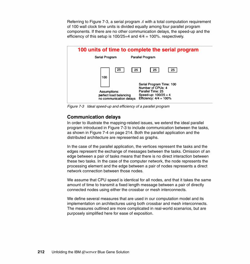
Referring to Figure 7-3, a serial program A with a total computation requirement of 100 wall clock time units is divided equally among four parallel program components. If there are no other communication delays, the speed-up and the efficiency of this setup is 100/25=4 and 4/4 = 100%. respectively.

Figure 7-3 Ideal speed-up and efficiency of a parallel program

Communication delaysIn order to illustrate the mapping-related issues, we extend the ideal parallel program introduced in Figure 7-3 to include communication between the tasks, as shown in Figure 7-4 on page 214. Both the parallel application and the distributed architecture are represented as graphs.

In the case of the parallel application, the vertices represent the tasks and the edges represent the exchange of messages between the tasks. Omission of an edge between a pair of tasks means that there is no direct interaction between these two tasks. In the case of the computer network, the node represents the processing element and the edge between a pair of nodes represents a direct network connection between those nodes.

We assume that CPU speed is identical for all nodes, and that it takes the same amount of time to transmit a fixed length message between a pair of directly connected nodes using either the crossbar or mesh interconnects.

We define several measures that are used in our computation model and its implementation on architectures using both crossbar and mesh interconnects. The measures outlined are more complicated in real-world scenarios, but are purposely simplified here for ease of exposition.

Serial Program Parallel Program

Assumptions: noperfect load balancing no communication delays

25252525

Serial Program Time: 100Number of CPUs: 4Parallel Time: 25Speed-up: 100/25 = 4Efficiency: 4/4 = 100%

100

Serial Program Parallel Program

Assumptions: noperfect load balancing no communication delays

25252525

Serial Program Time: 100Number of CPUs: 4Parallel Time: 25Speed-up: 100/25 = 4Efficiency: 4/4 = 100%

100

100 units of time to complete the serial program


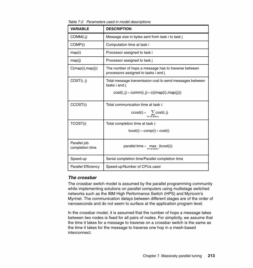
Table 7-2 Parameters used in model descriptions

The crossbarThe crossbar switch model is assumed by the parallel programming community while implementing solutions on parallel computers using multistage switched networks such as the IBM High Performance Switch (HPS) and Myricom’s Myrinet. The communication delays between different stages are of the order of nanoseconds and do not seem to surface at the application program level.

In the crossbar model, it is assumed that the number of hops a message takes between two nodes is fixed for all pairs of nodes. For simplicity, we assume that the time it takes for a message to traverse on a crossbar switch is the same as the time it takes for the message to traverse one hop in a mesh-based interconnect.

VARIABLE DESCRIPTION

COMM(i,j) Message size in bytes sent from task i to task j

COMP(i) Computation time at task i

map(i) Processor assigned to task i

map(j) Processor assigned to task j

C(map(i),map(j)) The number of hops a message has to traverse between processors assigned to tasks i and j

COST(i, j) Total message transmission cost to send messages between tasks i and j:

CCOST(i) Total communication time at task i:

TCOST(i) Total completion time at task i:

Parallel job completion time

Speed-up Serial completion time/Parallel completion time

Parallel Efficiency Speed-up/Number of CPUs used

map(j)))c((map(i),j)comm(i,j)cost(i, ×=

∑= j tasks all for

j)cost(i, ccost(i)

cost(i)comp(i)tcost(i) +=

(tcost(i))max time paralleli tasks all for

=


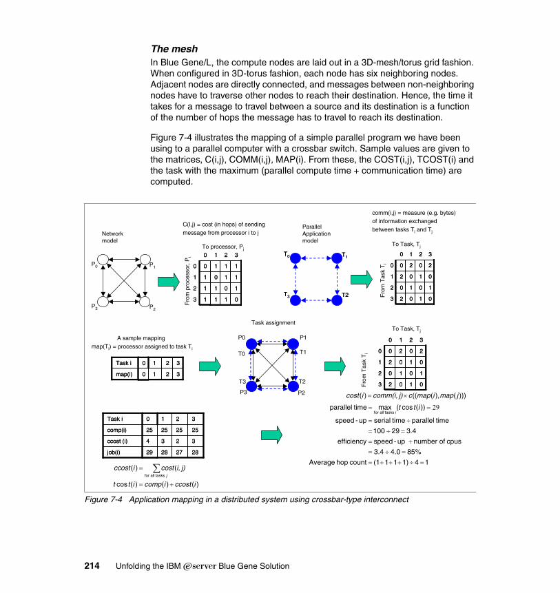
The meshIn Blue Gene/L, the compute nodes are laid out in a 3D-mesh/torus grid fashion. When configured in 3D-torus fashion, each node has six neighboring nodes. Adjacent nodes are directly connected, and messages between non-neighboring nodes have to traverse other nodes to reach their destination. Hence, the time it takes for a message to travel between a source and its destination is a function of the number of hops the message has to travel to reach its destination.

Figure 7-4 illustrates the mapping of a simple parallel program we have been using to a parallel computer with a crossbar switch. Sample values are given to the matrices, C(i,j), COMM(i,j), MAP(i). From these, the COST(i,j), TCOST(i) and the task with the maximum (parallel compute time + communication time) are computed.

Figure 7-4 Application mapping in a distributed system using crossbar-type interconnect

Network model

ParallelApplicationmodel

P0 P1

P3 P2

T0 T1

T3 T2

T0 T1

T3 T2

T0 T1

T3 T2

P0 P1

P3 P2

10112

11011

11100

01113

3210

10112

11011

11100

01113

3210

10102

01021

20200

01023

3210

10102

01021

20200

01023

3210

comm(i,j) = measure (e.g. bytes) of information exchanged between tasks Ti and Tj

C(I,j) = cost (in hops) of sending message from processor i to j

3210map(i)

3210Task i

3210map(i)

3210Task i

)()()(cos

( )( tasks all for

iccosticompitt

j)i,costiccostj

+=

= ∑

3234ccost (i)

25252525comp(i)

28272829job(i)

3210Task i

3234ccost (i)

25252525comp(i)

28272829job(i)

3210Task i

1 41)11(1 count hop Average

85% 4.0 3.4

cpus of number up-speed efficiency

3.4 29 100

time parallel time serialup-speed

))(cos(max time parallel tasks all for

=÷+++==÷=÷=

=÷=÷=

== 29itti

Fro

m p

roce

ssor

, Pi

To processor, Pj

Fro

m T

ask

Ti

To Task, Tj

10102

01021

20200

01023

3210

10102

01021

20200

01023

3210

)))(),((( )( jmapimapcj)comm(i,icost ×=

Fro

m T

ask

Ti

To Task, Tj

Task assignment

A sample mappingmap(Ti) = processor assigned to task Ti


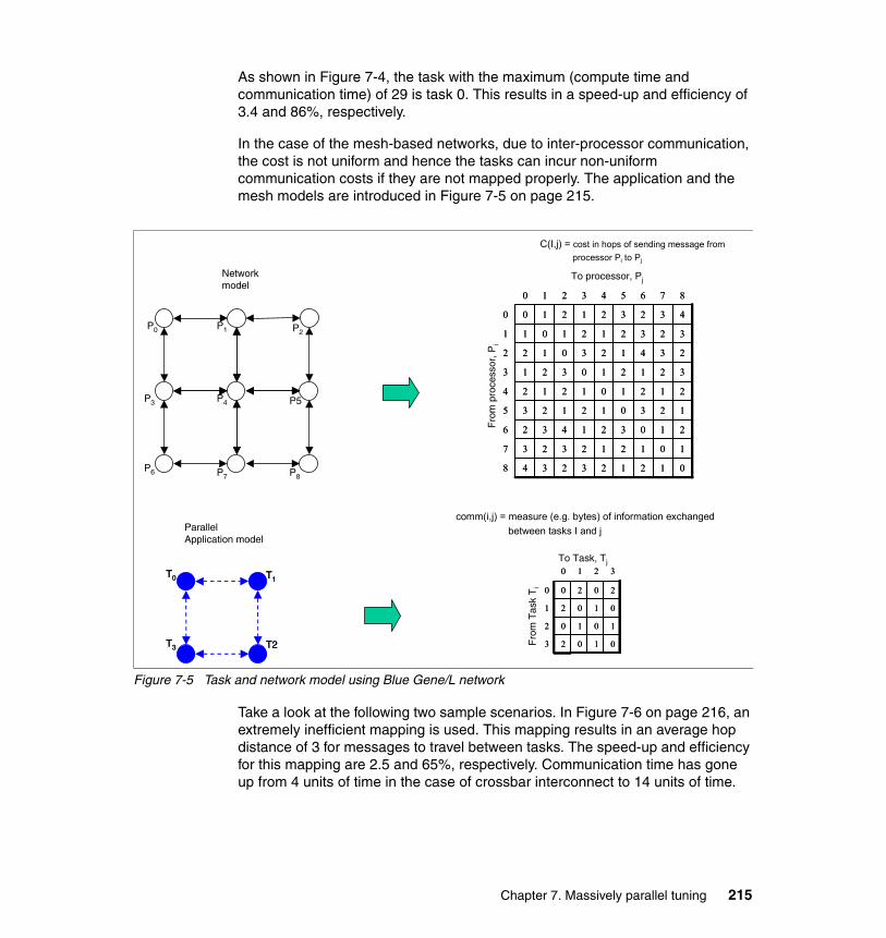
As shown in Figure 7-4, the task with the maximum (compute time and communication time) of 29 is task 0. This results in a speed-up and efficiency of 3.4 and 86%, respectively.

In the case of the mesh-based networks, due to inter-processor communication, the cost is not uniform and hence the tasks can incur non-uniform communication costs if they are not mapped properly. The application and the mesh models are introduced in Figure 7-5 on page 215.

Figure 7-5 Task and network model using Blue Gene/L network

Take a look at the following two sample scenarios. In Figure 7-6 on page 216, an extremely inefficient mapping is used. This mapping results in an average hop distance of 3 for messages to travel between tasks. The speed-up and efficiency for this mapping are 2.5 and 65%, respectively. Communication time has gone up from 4 units of time in the case of crossbar interconnect to 14 units of time.

Network model

ParallelApplication model

T0 T1

T3 T2

T0 T1

T3 T2

C(I,j) = cost in hops of sending message fromprocessor Pi to Pj

0121232348

1012123237

2103214326

1230121235

2121012124

3212103213

2341230122

3232121011

4323212100

876543210

0121232348

1012123237

2103214326

1230121235

2121012124

3212103213

2341230122

3232121011

4323212100

876543210

Fro

m p

roce

ssor

, Pi

To processor, Pj

P0

P6

P1

P3

P7

P4

P8

P2

P5

10102

01021

20200

01023

3210

10102

01021

20200

01023

3210

comm(i,j) = measure (e.g. bytes) of information exchanged between tasks I and j

Fro

m T

ask

Ti

To Task, Tj


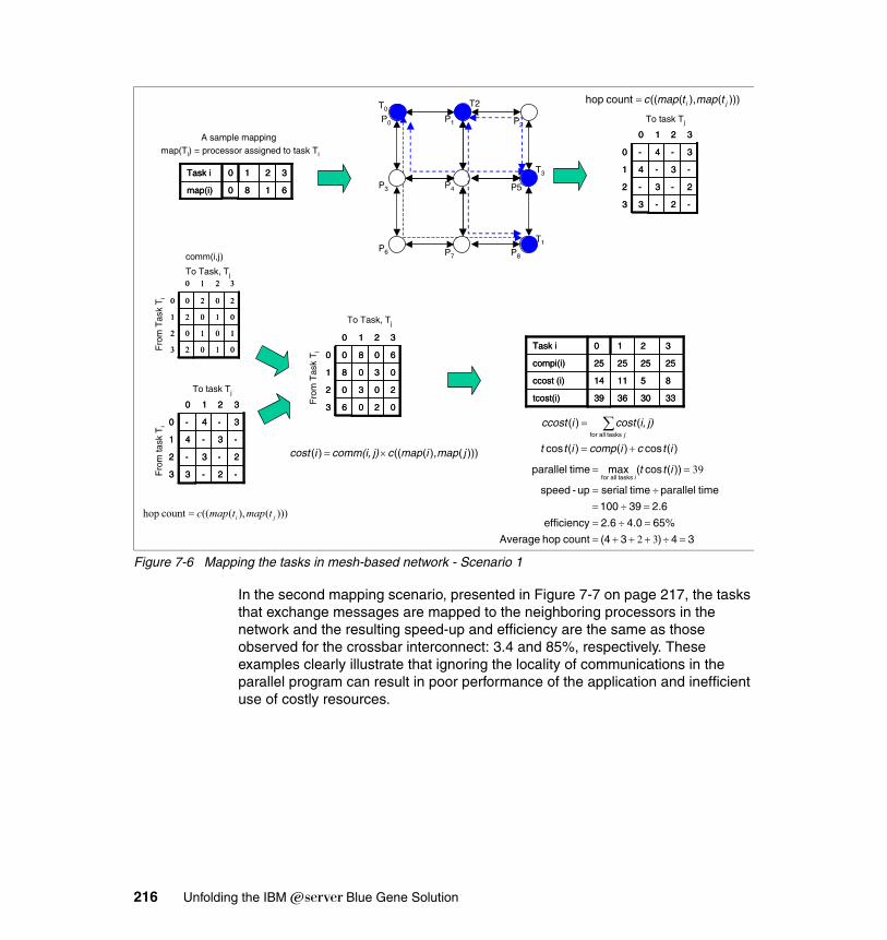
Figure 7-6 Mapping the tasks in mesh-based network - Scenario 1

In the second mapping scenario, presented in Figure 7-7 on page 217, the tasks that exchange messages are mapped to the neighboring processors in the network and the resulting speed-up and efficiency are the same as those observed for the crossbar interconnect: 3.4 and 85%, respectively. These examples clearly illustrate that ignoring the locality of communications in the parallel program can result in poor performance of the application and inefficient use of costly resources.

6180map(i)

3210Task i

6180map(i)

3210Task i

)(cos)()(cos

( )( tasks all for

itcicompitt

j)i,costiccostj

+=

= ∑

851114ccost (i)

25252525compi(i)

33303639tcost(i)

3210Task i

851114ccost (i)

25252525compi(i)

33303639tcost(i)

3210Task i


65% 4.0 2.6 efficiency

2.6 39 100



=÷+++==÷==÷=÷=

==

32

39itti

20302

03081

60800

02063

3210

20302

03081

60800

02063

3210


Fro

m T

ask

Ti

To Task, Tj

P0

P6

P1

P3

P7

P4

P8

P2

P5

T1

T3

)))(),((( count hop ji tmaptmapc=

2-3-2

-3-41

3-4-0

-2-33

3210

2-3-2

-3-41

3-4-0

-2-33

3210

To task Tj

T0T2

10102

01021

20200

01023

3210

10102

01021

20200

01023

3210

comm(i,j)

Fro

m T

ask

Ti

To Task, Tj


Fro

m ta

sk T

i

2-3-2

-3-41

3-4-0

-2-33

3210

2-3-2

-3-41

3-4-0

-2-33

3210

To task Tj



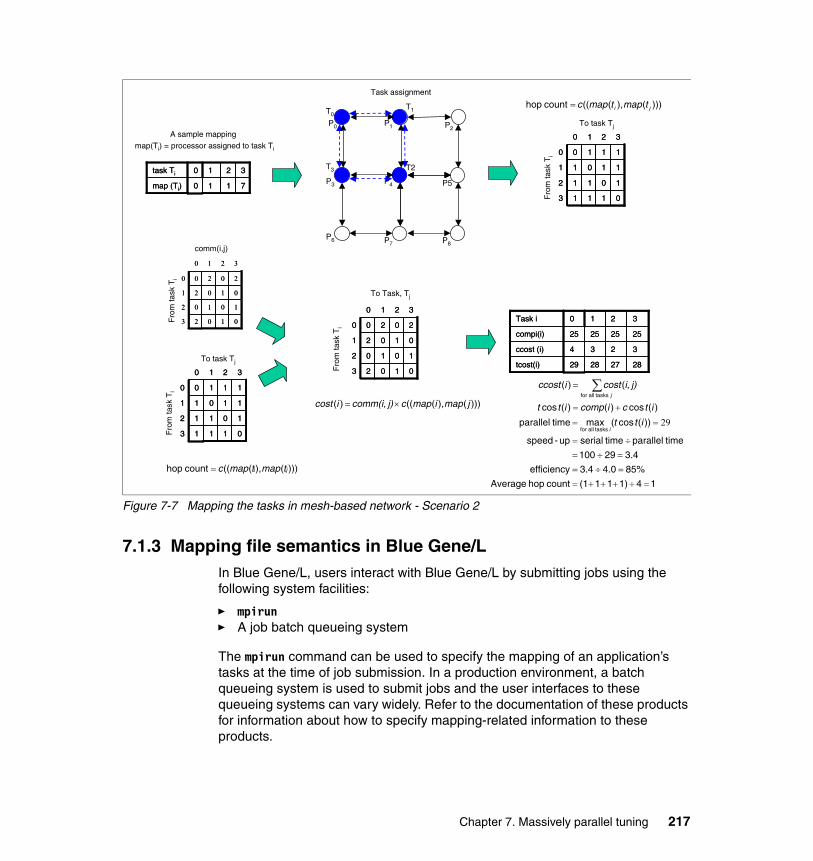
Figure 7-7 Mapping the tasks in mesh-based network - Scenario 2

7.1.3 Mapping file semantics in Blue Gene/LIn Blue Gene/L, users interact with Blue Gene/L by submitting jobs using the following system facilities:

� mpirun� A job batch queueing system

The mpirun command can be used to specify the mapping of an application’s tasks at the time of job submission. In a production environment, a batch queueing system is used to submit jobs and the user interfaces to these queueing systems can vary widely. Refer to the documentation of these products for information about how to specify mapping-related information to these products.


7110map (Ti)

3210task Ti

7110map (Ti)

3210task Ti

)(cos)()(cos

( )( tasks all for

itcicompitt

j)i,costiccostj

+=

= ∑

3234ccost (i)

25252525compi(i)

28272829tcost(i)

3210Task i

3234ccost (i)

25252525compi(i)

28272829tcost(i)

3210Task i


85% 4.0 3.4 efficiency

3.4 29 100



=÷+++==÷==÷=÷=

== 29itti

Fro

m ta

sk T

i

P0

P6

P1

P3

P7

P4

P8

P2

P5

T0T1

T3 T2

10112

11011

11100

01113

3210

10112

11011

11100

01113

3210

To task Tj

10102

01021

20200

01023

3210

10102

01021

20200

01023

3210


To Task, Tj

Fro

m ta

sk T

i

10102

01021

20200

01023

3210

10102

01021

20200

01023

3210

comm(i,j)

)))(),((( count hop i jtmaptmapc=

Fro

m ta

sk T

i

10112

11011

11100

01113

3210

10112

11011

11100

01113

3210

To task Tj

Fro

m ta

sk T

i

Task assignment



mpirunThe mpirun parameters that are relevant to application mapping are shown in Table 7-3.

Table 7-3 :Application mapping in Blue Gene/L

These parameters are used to specify to the system how to assign the tasks to processors. The Blue Gene/L partition allocated to the parallel application has a shape expressed as XxYxZ, where XYZ refers to the sizes of the partition’s X, Y, and Z axes, respectively.

For example, 16x8x8 refers to a partition of size 1024 nodes. Each of the compute nodes is given an absolute coordinate point starting from (0,0,0) and going all the way to (15,7,7).

The shape can either be user-specified (by giving a value to the shape parameter), or you can let the system choose the shape. If the partition is booted in coprocessor (CO) mode, only one processor per node is available for allocation, whereas if the partition is booted under virtual node (VN) mode, then both processors in the compute node are available for allocation.

After the partition shape is determined, the assignment of tasks to the processors is accomplished through the mapfile parameter.

Parameter Description

np Number of tasks

partition Name of partition (optional)

mapfile Method of mapping; one the following values (optional)� XYZT (default)� TXYZ� Absolute path of mapping file containing an entry for each of

the np tasks using the following format: – X Y Z T

shape Shape of job in compute nodes; format is XxYxZ

connect The connection type of the required partition, choices:TORUS or MESH (default=MESH)

mode Execution node mode of the required partition:� CO (coprocessor) (default)� VN (virtual node)

exe Full path of the parallel application executable


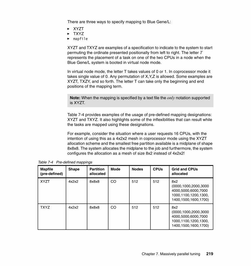
There are three ways to specify mapping to Blue Gene/L:

� XYZT� TXYZ� mapfile

XYZT and TXYZ are examples of a specification to indicate to the system to start permuting the ordinate presented positionally from left to right. The letter T represents the placement of a task on one of the two CPUs in a node when the Blue Gene/L system is booted in virtual node mode.

In virtual node mode, the letter T takes values of 0 or 1. In coprocessor mode it takes single value of 0. Any permutation of X,Y,Z is allowed. Some examples are XYZT, TXZY, and so forth. The letter T can take only the beginning and end positions of the mapping term.

Table 7-4 provides examples of the usage of pre-defined mapping designations: XYZT and TXYZ. It also highlights some of the inflexibilities that can result while the tasks are mapped using these designations.

For example, consider the situation where a user requests 16 CPUs, with the intention of using this as a 4x2x2 mesh in coprocessor mode using the XYZT allocation scheme and the smallest free partition available is a midplane of shape 8x8x8. The system allocates the midplane to the job and furthermore, the system configures the allocation as a mesh of size 8x2 instead of 4x2x2!

Table 7-4 Pre-defined mappings

Note: When the mapping is specified by a text file the only notation supported is XYZT.

Mapfile(pre-defined)

Shape Partition allocated

Mode Nodes CPUs Grid and CPUs allocated

XYZT 4x2x2 8x8x8 CO 512 512 8x2(0000,1000,2000,30004000,5000,6000,70001000,1100,1200,1300,1400,1500,1600,1700)

TXYZ 4x2x2 8x8x8 CO 512 512 8x2(0000,1000,2000,30004000,5000,6000,70001000,1100,1200,1300,1400,1500,1600,1700)


Blue Gene/L provides an additional mapping facility, giving users full flexibility of the placement, where users can designate exact placements of tasks on the compute nodes in a file. In this file, there is one entry for each task assignment and the designation follows the XYZT format as indicated below:

1 3 4 0

The entry instructs the system to place the task corresponding to this line in the map file on the first CPU of a compute node whose coordinates are (1,3,4); see Table 7-5. The number of lines in the mapfile should be equal to the number of tasks in the parallel program. There is a one-to-one mapping of line number in the mapfile and task number in the parallel program.

Table 7-5 Using custom mapping files

7.1.4 Automatic mapping methodsFor parallel applications that contain a large number of tasks, manual methods of analyzing traffic patterns and evaluating potential mapping scenarios are not

XYZT 4x2x2 8x8x8 VN 512 1024 8x2(0000,1000,2000,30004000,5000,6000,70001000,1100,1200,1300,1400,1500,1600,1700)

TXYZ 4x2x2 8x8x8 VN 512 1024 8x1(0000,0001,1000,1001,2000,2001,3000,30014000,4001,5000,5001,6000,6001,7000,7001)

Mapfile(pre-defined)



Mapfile(custom)



0000,0010,0100,0110,1000,1010,1100,11102000,2010,2100,2110,3000,3010,3100,3110

4x2x2 8x8x8 CO 512 512 4x2x2

0000,0001,0010,00110100,0101,0110,01111000,1001,1010,10111100,1101,1110,1111

4x2x2 8x8x8 VN 512 512 2x2x2


feasible and some automated mapping facilities are needed. In this section, we describe schemes that can be useful in mapping the tasks to Blue Gene/L processors. These methods are:

� Default allocation� Random allocation� Heuristic methods

Default allocationIn 7.1.3, “Mapping file semantics in Blue Gene/L” on page 217, we described the facilities provided by the Blue Gene/L system to map applications onto the Blue Gene/L system. These default mappings are recommended as a starting point when no information about inter-task communication in a parallel program is available. Information gathered about inter-task message patterns can then be used in either heuristic or optimal methods to further improve task assignment.

Random allocationIn the case of a parallel applications where either the message traffic patterns are not known a priori, or the message patterns change dynamically during job execution, a simple default assignment using the XYZT or random allocation of tasks to processors should suffice. In both cases, the average hop distances messages have to travel between tasks are very similar.

As shown in “Mapping using SAGE” on page 224, when the message traffic patterns are known, random placement can be very expensive compared to the heuristic techniques. Heuristic techniques attempt to use the information about the inter-task message patterns and can produce an assignment which preserves the locality communication between neighboring tasks in the parallel application.

Mapping based on heuristic methods For an n node system, the possible mappings which have to be searched for an optimal layout are O(n!). Clearly, it is not practical to enumerate all possible mappings. Methods to find optimal mappings can take a very long time to be useful. Heuristic methods, although provably not optimal in nature, provide a fast way to improve an existing solution.

Several heuristic methods have been proposed in the past to improve task assignment in large computer networks. In this section, we describe recent experiences with solving task assignment on Blue Gene/L system using heuristic methods. The first method is a simple heuristic that is very fast and generates good mappings when compared to random mappings. Then a more sophisticated method using the Simulated Annealing technique is introduced.


Mapping based on a simple heuristic Since the goal is to come up with a mapping that improves the cost function introduced in “Communication delays” on page 212, it is possible to come up with any number of heuristic algorithms to devise a solution from scratch or refine an exiting solution. Here is a simple heuristic that is used in the experiments and is labeled as “heuristic” in results presented later in this section.

A heuristic map is described by the following algorithm:

1. Let us assume the parallel program is divided into N tasks and is to be assigned to P processors on Blue Gene/L.

2. Map task i =1 to an arbitrary location (x, y, z).

3. Map all domains with which task i = 1 communicates either to location (x, y, z) or to its neighboring locations on the Blue Gene/L torus, while satisfying the constraint that only one task can be assigned to a processor.

4. Next, map task i = 2 (if it is not yet mapped) to an arbitrary location (x0; y0; z0) and the unmapped tasks with which it communicates either to the same node or to a neighboring node on the torus while satisfying the constraint that only one task can be allocated to a processor.

5. Repeat this last step for the remaining tasks i = 3; 4; :::;N.

This heuristic can be made more sophisticated by taking into account the volume of communication between tasks already allocated the remaining tasks. For example, in step 4, it is beneficial to map first those tasks with the greatest communication volume to already mapped tasks within their close proximity, rather than simply mapping in task rank order.

The output is in the format of the mapping file described in “Mapping file semantics in Blue Gene/L” on page 236.

Mapping based on simulated annealingAn algorithm that can be used to find an optimal mapping of parallel tasks to Blue Gene/L processors is presented in the article “Optimizing Task Layout on the Blue Gene/L Supercomputer”, Bhanot, et al, IBM September, 2004. This algorithm is used to minimize the communication delays for the entire parallel job. This approach uses a Simulated Annealing algorithm which takes into account the inter-task communication requirements and the inter-processor communication delays, and generates an optimal assignment of tasks for Blue Gene/L processors. The output of this algorithm is in the format of the mapping file described in 7.1.3, “Mapping file semantics in Blue Gene/L” on page 217.


The cost function the proposed algorithm attempts to minimize is given by the following formula:

where:

COMM(i,j) Message in bytes sent from task i to task jmap(i) Processor assigned to task imap(j) Processor assigned to task jC(map(i), map(j)) Inter-processor message transmission cost between

processor assigned to task, i and processor assigned to task, j

This procedure is called Simulated Annealing because it is analogous to the annealing processing in metallurgy, where metals are first heated and then slowly cooled to remove impurities.

Simulated annealing is an iterative method which repeatedly attempts to improve a given configuration by making random changes. To seed the process, an initial configuration must be set up. This can be selected at random or through a simple heuristic procedure such as the one described in “Mapping based on a simple heuristic” on page 222.

7.1.5 Manual mapping methodsIn some situations, the application designer may have knowledge about the communication behavior of the parallel application, but it may not be easily modeled for solving by automated mapping techniques. In these situations the mapping problem is solved through some manual analysis and the mapping is described to the Blue Gene/L system through the mapfile parameter.

For example, the application may exhibit different communication patterns during different stages of the program, and the application designer may decide to manually remap computations during the course of the execution of the parallel application.

In this section, we describe practical situations where manual analysis resulted in significantly improved performance over some of the automated techniques described in 7.1.4, “Automatic mapping methods” on page 220.

∑ ×= j i, tasks all for

map(j))c(map(i),j)comm(i, F


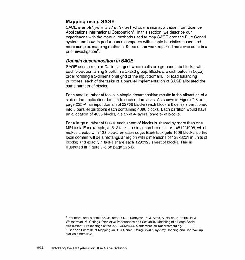
Mapping using SAGESAGE is an Adaptive Grid Eulerian hydrodynamics application from Science Applications International Corporation1. In this section, we describe our experiences with the manual methods used to map SAGE onto the Blue Gene/L system and how its performance compares with simple heuristics-based and more complex mapping methods. Some of the work reported here was done in a prior investigation2.

Domain decomposition in SAGESAGE uses a regular Cartesian grid, where cells are grouped into blocks, with each block containing 8 cells in a 2x2x2 group. Blocks are distributed in (x,y,z) order forming a 3-dimensional grid of the input domain. For load balancing purposes, each of the tasks of a parallel implementation of SAGE allocated the same number of blocks.

For a small number of tasks, a simple decomposition results in the allocation of a slab of the application domain to each of the tasks. As shown in Figure 7-8 on page 225-A, an input domain of 32768 blocks (each block is 8 cells) is partitioned into 8 parallel partitions each containing 4096 blocks. Each partition would have an allocation of 4096 blocks, a slab of 4 layers (sheets) of blocks.

For a large number of tasks, each sheet of blocks is shared by more than one MPI task. For example, at 512 tasks the total number of blocks =512*4096, which makes a cube with 128 blocks on each edge. Each task gets 4096 blocks, so the local domain will be a rectangular region with dimensions of 128x32x1 in units of blocks; and exactly 4 tasks share each 128x128 sheet of blocks. This is illustrated in Figure 7-8 on page 225-B.

1 For more details about SAGE, refer to D. J. Kerbyson, H. J. Alme, A. Hoisie, F. Petrini, H. J. Wasserman, M. Gittings,“Predictive Performance and Scalability Modeling of a Large-Scale Application”, Proceedings of the 2001 ACM/IEEE Conference on Supercomputing.2 See “An Example of Mapping on Blue Gene/L Using SAGE”, by Amy Henning and Bob Walkup, available from IBM.


Figure 7-8 Sample decompositions in SAGE

Once the logical grouping of input domain into subdomains is accomplished, the next step is to map this logical task set onto a Blue Gene/L architecture. Now, we describe a mapping that was used in a recent study to map the slab and strip decompositions onto a Blue Gene/L system.

Application mapping in SAGEIn the case of slab decomposition, boundary exchange involves communication with neighbors that are +/-1 in MPI task order. For a Blue Gene/L configured as a mesh, an example of a mapping with good locality would be a line that winds back and forth in the x-dimension, making a space-filling curve over the mesh network.

This ensures that all boundary exchange is to the nearest neighbors on the mesh. A disadvantage of this simple mapping is that only about one third of the links are used for communication. In principle, you could use a more complex mapping that gives up some locality in order to increase link utilization.

However, the slab decomposition is limited to small task counts with a modest communication requirement in the present example, and so a simple space filling curve is a good solution.

As the task count increases, more than one task shares each sheet of blocks, and the communication pattern becomes more complex. For the 512-CPU

A. B.SAGE slab decomposition for Decomposition for 512 MPI using8 MPI tasks, using 32768 cells 32768 cells per task. Eachper task. Each task has a local task has a local domain ofdomain of 32x32x4 blocks. 128x32x1 blocks.


example shown in Figure 7-8 on page 225-B, the most important communication step would be boundary exchange with tasks that are +/-4 in MPI task order.

To come up with a mapping file for this case, you could take a small square for a given x-coordinate on the torus, using the four points {(x,y,z), (x,y,z+1), (x,y+1,z+1), (x, y+1,z)}, and replicate this four-point patch in the x direction, winding through the torus network in a space-filling curve.

For 512 CPUs, this mapping has very good locality: the maximum distance between communicating pairs is 2 hops in torus coordinates, and the average distance is 1.07. The first few lines of the mapping file implementing four-point patch are listed below. For a description of the mapping file layout, see 7.1.3, “Mapping file semantics in Blue Gene/L” on page 217.

0 0 0 00 0 1 00 1 1 00 1 0 01 0 0 01 0 1 01 1 1 01 1 0 0

In the case of 2048 CPUs configured as a torus, a reasonably large problem can be mapped, with cells per CPU = 65536. The total number of blocks would be 2048*65536/8 = 16M = 256**3; so there would be a cube of blocks with 256 blocks along each edge, and 8 MPI tasks would share each sheet of blocks (8*256 = 2048). In this case, the communication pattern should be +/-1, and +/-8 in MPI rank; so the default XYZT mapping should be very good on an 8x8x32 torus. A sample mapfile containing the folding scheme described here is:

0 0 0 01 0 0 02 0 0 03 0 0 04 0 0 05 0 0 06 0 0 07 0 0 00 1 0 01 1 0 02 1 0 0

7.1.6 Mapping experimentsOn the same 512 CPU and 2048 CPU Blue Gene/L systems used in these experiments, in addition to the manual mapping scheme (labeled as the folding method), the following mapping methods were used for comparison. The results


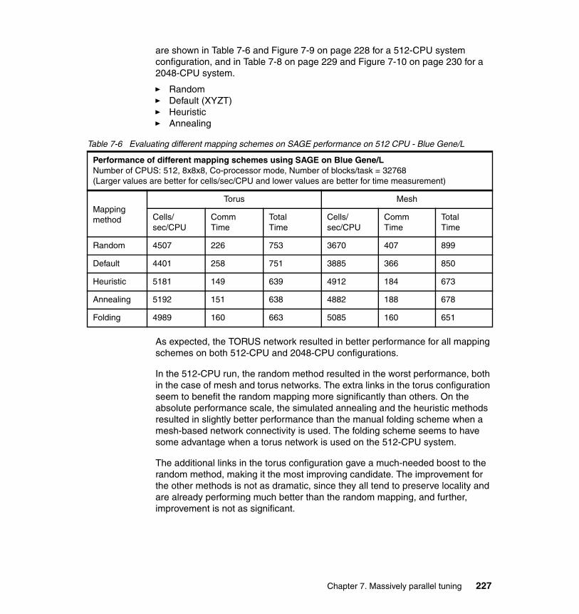
are shown in Table 7-6 and Figure 7-9 on page 228 for a 512-CPU system configuration, and in Table 7-8 on page 229 and Figure 7-10 on page 230 for a 2048-CPU system.

� Random� Default (XYZT)� Heuristic� Annealing

Table 7-6 Evaluating different mapping schemes on SAGE performance on 512 CPU - Blue Gene/L

As expected, the TORUS network resulted in better performance for all mapping schemes on both 512-CPU and 2048-CPU configurations.

In the 512-CPU run, the random method resulted in the worst performance, both in the case of mesh and torus networks. The extra links in the torus configuration seem to benefit the random mapping more significantly than others. On the absolute performance scale, the simulated annealing and the heuristic methods resulted in slightly better performance than the manual folding scheme when a mesh-based network connectivity is used. The folding scheme seems to have some advantage when a torus network is used on the 512-CPU system.

The additional links in the torus configuration gave a much-needed boost to the random method, making it the most improving candidate. The improvement for the other methods is not as dramatic, since they all tend to preserve locality and are already performing much better than the random mapping, and further, improvement is not as significant.

Performance of different mapping schemes using SAGE on Blue Gene/L Number of CPUS: 512, 8x8x8, Co-processor mode, Number of blocks/task = 32768(Larger values are better for cells/sec/CPU and lower values are better for time measurement)

Mapping method

Torus Mesh

Cells/sec/CPU

CommTime

TotalTime

Cells/sec/CPU

CommTime

TotalTime

Random 4507 226 753 3670 407 899

Default 4401 258 751 3885 366 850

Heuristic 5181 149 639 4912 184 673

Annealing 5192 151 638 4882 188 678

Folding 4989 160 663 5085 160 651


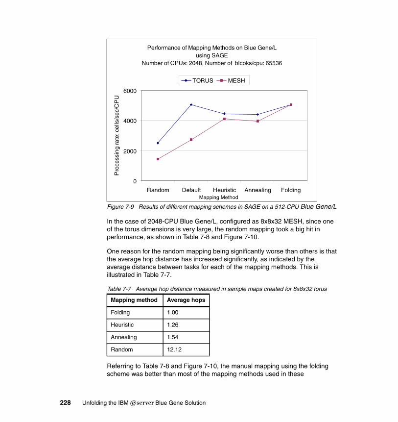
Figure 7-9 Results of different mapping schemes in SAGE on a 512-CPU Blue Gene/L

In the case of 2048-CPU Blue Gene/L, configured as 8x8x32 MESH, since one of the torus dimensions is very large, the random mapping took a big hit in performance, as shown in Table 7-8 and Figure 7-10.

One reason for the random mapping being significantly worse than others is that the average hop distance has increased significantly, as indicated by the average distance between tasks for each of the mapping methods. This is illustrated in Table 7-7.

Table 7-7 Average hop distance measured in sample maps created for 8x8x32 torus

Referring to Table 7-8 and Figure 7-10, the manual mapping using the folding scheme was better than most of the mapping methods used in these

Mapping method Average hops

Folding 1.00

Heuristic 1.26

Annealing 1.54

Random 12.12

Performance of Mapping Methods on Blue Gene/Lusing SAGE

Number of CPUs: 2048, Number of blcoks/cpu: 65536

0

2000

4000

6000

Random Default Heuristic Annealing FoldingMapping Method

Pro

cess

ing

rate

: cel

ls/s

ec/C

PU

TORUS MESH


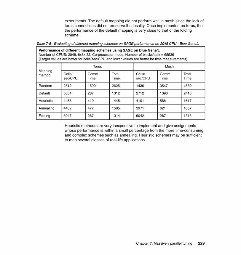
experiments. The default mapping did not perform well in mesh since the lack of torus connections did not preserve the locality. Once implemented on torus, the the performance of the default mapping is very close to that of the folding scheme.

Table 7-8 Evaluating of different mapping schemes on SAGE performance on 2048 CPU - Blue Gene/L

Heuristic methods are very inexpensive to implement and give assignments whose performance is within a small percentage from the more time-consuming and complex schemes such as annealing. Heuristic schemes may be sufficient to map several classes of real-life applications.

Performance of different mapping schemes using SAGE on Blue Gene/L Number of CPUS: 2048, 8x8x,32, Co-processor mode, Number of blocks/task = 65536(Larger values are better for cells/sec/CPU and lower values are better for time measurements)

Mapping method

Torus Mesh

Cells/sec/CPU

CommTime

TotalTime

Cells/sec/CPU

CommTime

TotalTime

Random 2512 1590 2625 1436 3547 4580

Default 5054 287 1312 2712 1390 2418

Heuristic 4455 419 1445 4101 588 1617

Annealing 4402 477 1505 3971 621 1657

Folding 5047 287 1314 5042 287 1315


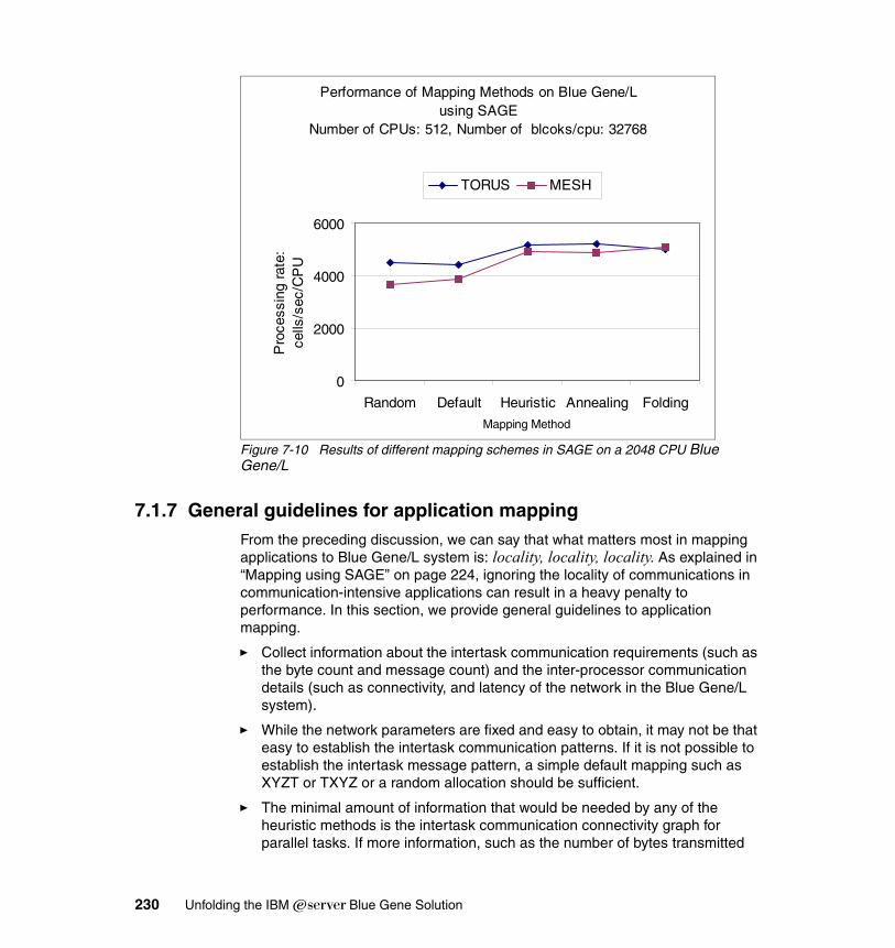
Figure 7-10 Results of different mapping schemes in SAGE on a 2048 CPU Blue Gene/L

7.1.7 General guidelines for application mappingFrom the preceding discussion, we can say that what matters most in mapping applications to Blue Gene/L system is: locality, locality, locality. As explained in “Mapping using SAGE” on page 224, ignoring the locality of communications in communication-intensive applications can result in a heavy penalty to performance. In this section, we provide general guidelines to application mapping.

� Collect information about the intertask communication requirements (such as the byte count and message count) and the inter-processor communication details (such as connectivity, and latency of the network in the Blue Gene/L system).

� While the network parameters are fixed and easy to obtain, it may not be that easy to establish the intertask communication patterns. If it is not possible to establish the intertask message pattern, a simple default mapping such as XYZT or TXYZ or a random allocation should be sufficient.

� The minimal amount of information that would be needed by any of the heuristic methods is the intertask communication connectivity graph for parallel tasks. If more information, such as the number of bytes transmitted

Performance of Mapping Methods on Blue Gene/Lusing SAGE

Number of CPUs: 512, Number of blcoks/cpu: 32768

0

2000

4000

6000

Random Default Heuristic Annealing Folding

Mapping Method

Pro

cess

ing

rate

: ce

lls/s

ec/C

PU

TORUS MESH


and the frequency of communication is available, then mapping methods similar to the ones described in 7.1.4, “Automatic mapping methods” on page 220 can produce better mappings.

� Simple heuristic-based mapping methods can result in significant improvement over either random or default mapping schemes. Further refinement may need more complex and costly methods.

Sometimes, as illustrated in “Mapping using SAGE” on page 224, analysts who are familiar with the communication patterns of an application may be able to spot a good mapping, which will be very hard to improve further using the heuristic methods.

7.1.8 MPI topologies and Cartesian communicatorsThe previously described methods of explicitly mapping MPI tasks to torus coordinates through a mapfile are external to the application. They can help to optimize communication performance by studying MPI traces of running applications, and then adequately remapping the tasks on the torus for subsequent runs.

However, they ignore the fact that the application itself may have inherent topological characteristics that can be expressed by MPI constructs. Those could be exploited by the MPI runtime system without the need for additional (manual or automatic) mapping. In this section we discuss the techniques that can be used inside the application to express such properties.

The MPI topologies frameworkChapter 6 of the MPI 1.1 standard (MPI - A Message Passing Interface Standard. Message Passing Interface Forum. June 12, 1995.) covers MPI topologies. This is a seldom used part of MPI, both because its use requires some initial learning curve, and because most current parallel computers have crossbar switches which are less susceptible to task placement than a torus topology.

The idea underlying the MPI topologies framework is to attach some knowledge of the topology of the application’s communication patterns to an MPI communicator. To achieve this, MPI 1.1 defines functions that can create a new communicator by using an existing communicator (typically MPI_COMM_WORLD) and parameters describing the desired topology as input. There are two classes of functions, one for general graphs and a second one for


Cartesian topologies. Here we only discuss the Cartesian case, for the following reasons:

� Many scientific/technical applications naturally map to some Cartesian space, while relatively few applications need general graphs to express their communication patterns.

� The torus network of the Blue Gene/L system is Cartesian.

� The Blue Gene/L MPI library only provides optimized functions for Cartesian topologies (a direct consequence of the preceding).

In addition to the creation of a Cartesian communicator, MPI also provides functions which inquire the topology information attached to a communicator, and conversion routines to translate between the Cartesian coordinates and the flat MPI rank. Finally, similar to MPI_Comm_Split() which can be used to partition a non-topological communicator, MPI_Cart_Sub() can be used to partition a Cartesian communicator into lower-dimensional Cartesian subgrids.

Using Cartesian communicators has several advantages:

� The MPI library can automatically optimize the placement of tasks on the torus, based on the topology information attached to the Cartesian communicator.

� Many communication patterns can be expressed more elegantly by using Cartesian coordinates than by using the flat MPI rank and some hand-crafted indexing scheme.

� Using special communicators (for example, rows on the torus), collective communications across such a communicator may exploit BG/L-specific hardware support (like multicasts along a torus axis) which would otherwise not be easily possible.

At the time of writing, the MPI library provides optimized MPI topology support within the following limits:

� The communicator used as the input communicator to MPI_Cart_Create() must represent a rectangular part of the torus network.

Note: For completeness, the Blue Gene/L MPI library provides all MPI topology functions, including those for graphs. But the graph-related functions do not actually perform any optimization. Starting with BG/L driver level 280, some support for optimization of Cartesian communicators has been introduced and this section is based on a preliminary version of that MPI library.


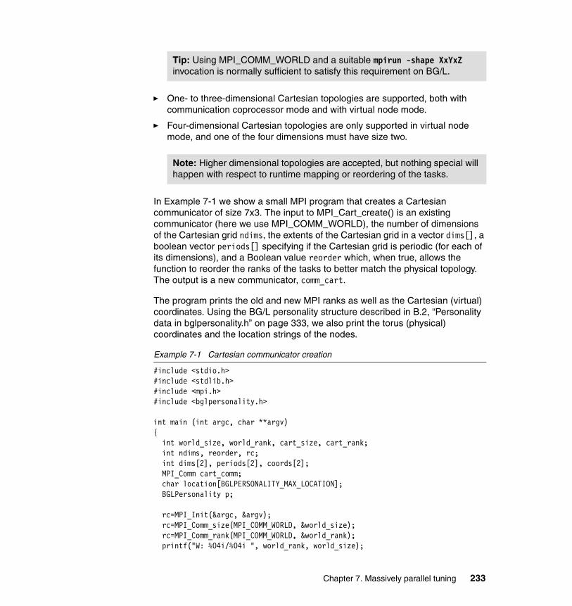
� One- to three-dimensional Cartesian topologies are supported, both with communication coprocessor mode and with virtual node mode.

� Four-dimensional Cartesian topologies are only supported in virtual node mode, and one of the four dimensions must have size two.

In Example 7-1 we show a small MPI program that creates a Cartesian communicator of size 7x3. The input to MPI_Cart_create() is an existing communicator (here we use MPI_COMM_WORLD), the number of dimensions of the Cartesian grid ndims, the extents of the Cartesian grid in a vector dims[], a boolean vector periods[] specifying if the Cartesian grid is periodic (for each of its dimensions), and a Boolean value reorder which, when true, allows the function to reorder the ranks of the tasks to better match the physical topology. The output is a new communicator, comm_cart.

The program prints the old and new MPI ranks as well as the Cartesian (virtual) coordinates. Using the BG/L personality structure described in B.2, “Personality data in bglpersonality.h” on page 333, we also print the torus (physical) coordinates and the location strings of the nodes.

Example 7-1 Cartesian communicator creation

#include <stdio.h>#include <stdlib.h>#include <mpi.h>#include <bglpersonality.h>

int main (int argc, char **argv){ int world_size, world_rank, cart_size, cart_rank; int ndims, reorder, rc; int dims[2], periods[2], coords[2]; MPI_Comm cart_comm; char location[BGLPERSONALITY_MAX_LOCATION]; BGLPersonality p;

rc=MPI_Init(&argc, &argv); rc=MPI_Comm_size(MPI_COMM_WORLD, &world_size); rc=MPI_Comm_rank(MPI_COMM_WORLD, &world_rank); printf("W: %04i/%04i ", world_rank, world_size);

Tip: Using MPI_COMM_WORLD and a suitable mpirun -shape XxYxZ invocation is normally sufficient to satisfy this requirement on BG/L.

Note: Higher dimensional topologies are accepted, but nothing special will happen with respect to runtime mapping or reordering of the tasks.


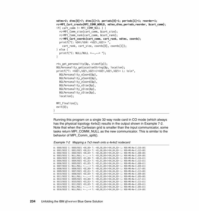
ndims=2; dims[0]=7; dims[1]=3; periods[0]=1; periods[1]=1; reorder=1;rc=MPI_Cart_create(MPI_COMM_WORLD, ndims,dims,periods,reorder, &cart_comm);

if( cart_comm != MPI_COMM_NULL ) { rc=MPI_Comm_size(cart_comm, &cart_size); rc=MPI_Comm_rank(cart_comm, &cart_rank); rc=MPI_Cart_coords(cart_comm, cart_rank, ndims, coords); printf("C: %04i/%04i <%02i,%02i> ", cart_rank, cart_size, coords[0], coords[1]); } else { printf("C: NULL/NULL <--,--> "); }

rts_get_personality(&p, sizeof(p)); BGLPersonality_getLocationString(&p, location); printf("T: <%02i,%02i,%02i>/<%02i,%02i,%02i> L: %s\n",

BGLPersonality_xCoord(&p),BGLPersonality_yCoord(&p),BGLPersonality_zCoord(&p),BGLPersonality_xSize(&p),BGLPersonality_ySize(&p),BGLPersonality_zSize(&p),

location);

MPI_Finalize(); exit(0);}

Running this program on a single 32-way node card in CO mode (which always has the physical topology 4x4x2) results in the output shown in Example 7-2. Note that when the Cartesian grid is smaller than the input communicator, some tasks return MPI_COMM_NULL as the new communicator. This is similar to the behavior of MPI_Comm_split().

Example 7-2 Mapping a 7x3 mesh onto a 4x4x2 nodecard

W: 0000/0032 C: 0000/0021 <00,00> T: <00,00,00>/<04,04,02> L: R00-M0-Ne-C:J16-U01W: 0001/0032 C: 0001/0021 <00,01> T: <01,00,00>/<04,04,02> L: R00-M0-Ne-C:J12-U01W: 0002/0032 C: 0002/0021 <00,02> T: <02,00,00>/<04,04,02> L: R00-M0-Ne-C:J08-U01W: 0003/0032 C: NULL/NULL <--,--> T: <03,00,00>/<04,04,02> L: R00-M0-Ne-C:J04-U01W: 0004/0032 C: 0003/0021 <01,00> T: <00,01,00>/<04,04,02> L: R00-M0-Ne-C:J16-U11W: 0005/0032 C: 0004/0021 <01,01> T: <01,01,00>/<04,04,02> L: R00-M0-Ne-C:J12-U11W: 0006/0032 C: 0005/0021 <01,02> T: <02,01,00>/<04,04,02> L: R00-M0-Ne-C:J08-U11W: 0007/0032 C: NULL/NULL <--,--> T: <03,01,00>/<04,04,02> L: R00-M0-Ne-C:J04-U11W: 0008/0032 C: 0006/0021 <02,00> T: <00,02,00>/<04,04,02> L: R00-M0-Ne-C:J17-U01W: 0009/0032 C: 0007/0021 <02,01> T: <01,02,00>/<04,04,02> L: R00-M0-Ne-C:J13-U01W: 0010/0032 C: 0008/0021 <02,02> T: <02,02,00>/<04,04,02> L: R00-M0-Ne-C:J09-U01W: 0011/0032 C: NULL/NULL <--,--> T: <03,02,00>/<04,04,02> L: R00-M0-Ne-C:J05-U01W: 0012/0032 C: 0009/0021 <03,00> T: <00,03,00>/<04,04,02> L: R00-M0-Ne-C:J17-U11W: 0013/0032 C: 0010/0021 <03,01> T: <01,03,00>/<04,04,02> L: R00-M0-Ne-C:J13-U11W: 0014/0032 C: 0011/0021 <03,02> T: <02,03,00>/<04,04,02> L: R00-M0-Ne-C:J09-U11W: 0015/0032 C: NULL/NULL <--,--> T: <03,03,00>/<04,04,02> L: R00-M0-Ne-C:J05-U11W: 0016/0032 C: NULL/NULL <--,--> T: <00,00,01>/<04,04,02> L: R00-M0-Ne-C:J14-U01


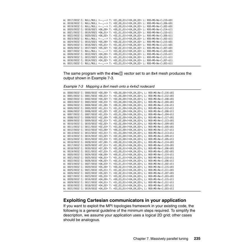
W: 0017/0032 C: NULL/NULL <--,--> T: <01,00,01>/<04,04,02> L: R00-M0-Ne-C:J10-U01W: 0018/0032 C: NULL/NULL <--,--> T: <02,00,01>/<04,04,02> L: R00-M0-Ne-C:J06-U01W: 0019/0032 C: NULL/NULL <--,--> T: <03,00,01>/<04,04,02> L: R00-M0-Ne-C:J02-U01W: 0020/0032 C: 0018/0021 <06,00> T: <00,01,01>/<04,04,02> L: R00-M0-Ne-C:J14-U11W: 0021/0032 C: 0019/0021 <06,01> T: <01,01,01>/<04,04,02> L: R00-M0-Ne-C:J10-U11W: 0022/0032 C: 0020/0021 <06,02> T: <02,01,01>/<04,04,02> L: R00-M0-Ne-C:J06-U11W: 0023/0032 C: NULL/NULL <--,--> T: <03,01,01>/<04,04,02> L: R00-M0-Ne-C:J02-U11W: 0024/0032 C: 0015/0021 <05,00> T: <00,02,01>/<04,04,02> L: R00-M0-Ne-C:J15-U01W: 0025/0032 C: 0016/0021 <05,01> T: <01,02,01>/<04,04,02> L: R00-M0-Ne-C:J11-U01W: 0026/0032 C: 0017/0021 <05,02> T: <02,02,01>/<04,04,02> L: R00-M0-Ne-C:J07-U01W: 0027/0032 C: NULL/NULL <--,--> T: <03,02,01>/<04,04,02> L: R00-M0-Ne-C:J03-U01W: 0028/0032 C: 0012/0021 <04,00> T: <00,03,01>/<04,04,02> L: R00-M0-Ne-C:J15-U11W: 0029/0032 C: 0013/0021 <04,01> T: <01,03,01>/<04,04,02> L: R00-M0-Ne-C:J11-U11W: 0030/0032 C: 0014/0021 <04,02> T: <02,03,01>/<04,04,02> L: R00-M0-Ne-C:J07-U11W: 0031/0032 C: NULL/NULL <--,--> T: <03,03,01>/<04,04,02> L: R00-M0-Ne-C:J03-U11

The same program with the dims[] vector set to an 8x4 mesh produces the output shown in Example 7-3.

Example 7-3 Mapping a 8x4 mesh onto a 4x4x2 nodecard

W: 0000/0032 C: 0000/0032 <00,00> T: <00,00,00>/<04,04,02>; L: R00-M0-Ne-C:J16-U01W: 0001/0032 C: 0001/0032 <00,01> T: <01,00,00>/<04,04,02>; L: R00-M0-Ne-C:J12-U01W: 0002/0032 C: 0002/0032 <00,02> T: <02,00,00>/<04,04,02>; L: R00-M0-Ne-C:J08-U01W: 0003/0032 C: 0003/0032 <00,03> T: <03,00,00>/<04,04,02>; L: R00-M0-Ne-C:J04-U01W: 0004/0032 C: 0004/0032 <01,00> T: <00,01,00>/<04,04,02>; L: R00-M0-Ne-C:J16-U11W: 0005/0032 C: 0005/0032 <01,01> T: <01,01,00>/<04,04,02>; L: R00-M0-Ne-C:J12-U11W: 0006/0032 C: 0006/0032 <01,02> T: <02,01,00>/<04,04,02>; L: R00-M0-Ne-C:J08-U11W: 0007/0032 C: 0007/0032 <01,03> T: <03,01,00>/<04,04,02>; L: R00-M0-Ne-C:J04-U11W: 0008/0032 C: 0008/0032 <02,00> T: <00,02,00>/<04,04,02>; L: R00-M0-Ne-C:J17-U01W: 0009/0032 C: 0009/0032 <02,01> T: <01,02,00>/<04,04,02>; L: R00-M0-Ne-C:J13-U01W: 0010/0032 C: 0010/0032 <02,02> T: <02,02,00>/<04,04,02>; L: R00-M0-Ne-C:J09-U01W: 0011/0032 C: 0011/0032 <02,03> T: <03,02,00>/<04,04,02>; L: R00-M0-Ne-C:J05-U01W: 0012/0032 C: 0012/0032 <03,00> T: <00,03,00>/<04,04,02>; L: R00-M0-Ne-C:J17-U11W: 0013/0032 C: 0013/0032 <03,01> T: <01,03,00>/<04,04,02>; L: R00-M0-Ne-C:J13-U11W: 0014/0032 C: 0014/0032 <03,02> T: <02,03,00>/<04,04,02>; L: R00-M0-Ne-C:J09-U11W: 0015/0032 C: 0015/0032 <03,03> T: <03,03,00>/<04,04,02>; L: R00-M0-Ne-C:J05-U11W: 0016/0032 C: 0028/0032 <07,00> T: <00,00,01>/<04,04,02>; L: R00-M0-Ne-C:J14-U01W: 0017/0032 C: 0029/0032 <07,01> T: <01,00,01>/<04,04,02>; L: R00-M0-Ne-C:J10-U01W: 0018/0032 C: 0030/0032 <07,02> T: <02,00,01>/<04,04,02>; L: R00-M0-Ne-C:J06-U01W: 0019/0032 C: 0031/0032 <07,03> T: <03,00,01>/<04,04,02>; L: R00-M0-Ne-C:J02-U01W: 0020/0032 C: 0024/0032 <06,00> T: <00,01,01>/<04,04,02>; L: R00-M0-Ne-C:J14-U11W: 0021/0032 C: 0025/0032 <06,01> T: <01,01,01>/<04,04,02>; L: R00-M0-Ne-C:J10-U11W: 0022/0032 C: 0026/0032 <06,02> T: <02,01,01>/<04,04,02>; L: R00-M0-Ne-C:J06-U11W: 0023/0032 C: 0027/0032 <06,03> T: <03,01,01>/<04,04,02>; L: R00-M0-Ne-C:J02-U11W: 0024/0032 C: 0020/0032 <05,00> T: <00,02,01>/<04,04,02>; L: R00-M0-Ne-C:J15-U01W: 0025/0032 C: 0021/0032 <05,01> T: <01,02,01>/<04,04,02>; L: R00-M0-Ne-C:J11-U01W: 0026/0032 C: 0022/0032 <05,02> T: <02,02,01>/<04,04,02>; L: R00-M0-Ne-C:J07-U01W: 0027/0032 C: 0023/0032 <05,03> T: <03,02,01>/<04,04,02>; L: R00-M0-Ne-C:J03-U01W: 0028/0032 C: 0016/0032 <04,00> T: <00,03,01>/<04,04,02>; L: R00-M0-Ne-C:J15-U11W: 0029/0032 C: 0017/0032 <04,01> T: <01,03,01>/<04,04,02>; L: R00-M0-Ne-C:J11-U11W: 0030/0032 C: 0018/0032 <04,02> T: <02,03,01>/<04,04,02>; L: R00-M0-Ne-C:J07-U11W: 0031/0032 C: 0019/0032 <04,03> T: <03,03,01>/<04,04,02>; L: R00-M0-Ne-C:J03-U11

Exploiting Cartesian communicators in your applicationIf you want to exploit the MPI topologies framework in your existing code, the following is a general guideline of the minimum steps required. To simplify the description, we assume your application uses a logical 2D grid; other cases should be analogous.


1. In your main program, declare a communicator variable, type MPI_Comm in C/C++ or type default INTEGER in Fortran.

2. Assign this variable the (constant) value of MPI_COMM_WORLD.

3. Replace all instances of MPI_COMM_WORLD in your MPI calls with the variable you just created. After this change, the application should still behave exactly the same, but now you can easily change the communicator by modifying the variable.

4. Create a suitable Cartesian communicator for your logical 2D grid by calling MPI_Cart_create() with reorder set to true. Use the communicator variable declared in step 1 as the output argument.

By allowing MPI_Cart_create() to reorder the ranks of the tasks, you will get a rank ordering in the new communicator that will “naturally” reflect the desired Cartesian grid. As long as your manual conversion of MPI rank to Cartesian coordinate in the application code follows a regular scheme (like row-major), you will get good locality in the Cartesian grid simply by using the new communicator in all your point-to-point communications instead of MPI_COMM_WORLD. This is typically a very small source code change.

If you want to invest more time into MPI topologies, you can replace your manual MPI rank to coordinate translation with the appropriate MPI_Cart_coords() and MPI_Cart_rank() functions, and neighbor addressing with MPI_Cart_shift(). Often this makes the MPI calls more readable, but it also is more work. Newly written codes can and should make use of these extended features, because expressing your algorithms in their natural topology is much clearer and offers good opportunities for runtime optimization.

Partitioning Cartesian communicatorsWhile MPI_Cart_create() gives you the ability to exploit locality for the point-to-point communications, there is another useful application for Cartesian communicators: Assume you need to perform some sort of collective communication within a subspace of the Cartesian grid (like a broadcast along a row or a column in a 2D grid). Normally you would use hand-crafted point-to-point messages along these rows/columns. But alternatively, you can use the MPI_Cart_sub() function to further partition your Cartesian communicator, and then use collective communications across these smaller communicators.

Note: Do this after MPI_Init(), but before any message passing calls and before any calculations based on MPI_Comm_Size() nor MPI_Comm_rank(). This is important because the rank of your local tasks will likely change.


In general, collective operations use the tree network if they are performed in the MPI_COMM_WORLD space. They fall back to the torus network for arbitrary communicators. However, if you use suitable Cartesian communicators you may be able to benefit from special hardware features of the torus network, like its ability to issue multicasts along any axis of the torus network.

A very common task in a parallel application is to broadcast data across a row or column in a 2D mesh, or to perform some reduction across a row or column (like finding the maximum value in a row). In the following we show how to partition a 2D Cartesian communicator into sets of row-communicators and column-communicators, and how to perform collective communications using these Cartesian sub-spaces. Using the declarations from Example 7-1 on page 233, we first create a 6x8 Cartesian communicator cart_comm:

ndims=2; dims[0]=6; dims[1]=8; periods[0]=0; periods[1]=0; reorder=1;rc=MPI_Cart_create(MPI_COMM_WORLD, ndims,dims,periods,reorder, &cart_comm);

Next we create row-communicators by using MPI_Cart_sub(), keeping the first dimension and dropping the second dimension of cart_comm:

MPI_Comm cart_row, cart_col;int remain_dims[2]; /* logical vector of which dims to keep/drop */

remain_dims[0]=1; remain_dims[1]=0;rc=MPI_Cart_sub(cart_comm, remain_dims, &cart_row);

Similarly, column communicators can be created by dropping the first dimension and keeping the second dimension:

remain_dims[0]=0; remain_dims[1]=1;rc=MPI_Cart_sub(cart_comm, remain_dims, &cart_col);

For each task in the 2D mesh, these new communicators will contain all the tasks in the same row/column as the local task. Conversely, the communicator handlers for cart_row will be different in different rows, and those for cart_col will be different in different columns.

You can now use these one-dimensional communicators to perform collective operations along one axis of your logical grid. For example:

� Reduction operation (MPI_MAX) along a column communicator:

rc=MPI_Reduce(send_buf, recv_buf, count, MPI_INT, MPI_MAX, root_rank, cart_row);

� Broadcasting along a row communicator:

rc=MPI_Bcast(buf, count, MPI_REAL, root_rank, cart_row);

If your logical 2D grid is adequately mapped to the physical torus network, those collectives may be able to exploit the special hardware features of the torus


network like its multicast capabilities. Of course, if the mapping does not fit the physical topology, the collectives will fall back to a standard implementation using only standard point-to-point calls underneath.

7.2 Limitations on scalingIn this section, we discuss a way of estimating the number of CPUs an application will be able to scale to.

With all parallel applications, if we assume that the serial section of a code is insignificant, it is the use of the network which dictates whether a code will scale up to many thousands of CPUs efficiently. To illustrate the different scaling of an application, we shall use the following example. For a general three-dimensional N by N problem with the number of variables N=K*L*M in three dimensions and processors P=xyz, the communication efficiency can be written (if we assume that the communication and computation do not overlap), as:

For the BG/L system, this can be written as:

Equation 1: Theoretical communication efficiency:

Where:

x P/NF Flops/variableB Bytes/variable to/from neighbor processorf Processing speed in flops/s = 2.8GFlops/sc Compute efficiency = 2d Latency = 10 μSecb Bandwidth = 1.4Gb/se Communication efficiency = 0.5

In Equation 1, the latency is represented by 6d(fc/F)x and the bandwidth by 6(c/e)*(fB/Fb)x^(1/3).

Efficency ComputeTimeComputeTime CommunicationTime+------------------------------------------------------------------------------------------------------------=

E 1

1 6d fcF---⎝ ⎠

⎛ ⎞ x 6 ce---⎝ ⎠⎛ ⎞ f B

Fb-------⎝ ⎠

⎛ ⎞ x1 3/++

----------------------------------------------------------------------------=

⎝ ⎠⎜ ⎟⎜ ⎟⎜ ⎟⎛ ⎞


With parallel applications, there are two scenarios in which we could exploit BG/L:

� Scenario 1

BG/L can be exploited when the total problem size is fixed and the problem size per processor drops as the number of processors increases. This means that for any N, eventually P will dominate.

It can be seen from equation 1 that large values of N are best suited for this scenario. Examples of applications that exhibit this type of scaling include protein folding, weather modeling, Quantum Chrono-Dynamics (QCD), seismic processing, and Computational Fluid Dynamics (CFD).

� Scenario 2

The other scenario in which to exploit the BGL system is when the problem size per processor is fixed with increasing processor numbers. Examples of codes that follow this type of scaling are Linpack, Stream, and SPPM. This means that the latency dominates when the second term in the denominator of equation 1 increases and the following two conditions are met:

x > 5e-6 (f/c), andx > 5e-6(B/e)^(3/2)

Using this, we can predict when an application will fail to scale:

� F = B = 1. This is the case of transaction processing and will become latency-bound when N/P < 200,000.

� F = 100, B = 1. This case will be come latency-bound if N/P < 2000.

� F = 1000, B = 100. This case will be latency-bound if N/P < 200.

7.3 Hints on how to parallelize codes The following sections provide hints on how to maximize the performance of an application on BG/L. These ideas came to light during the porting of applications covered in Chapter 8, “Applications on Blue Gene” on page 249.

7.3.1 All-to-all communicationFor a general massively parallel system which uses a single cross-bar switch, the time for performing an MPI all-to-all communication can be written as shown in Equation 2.


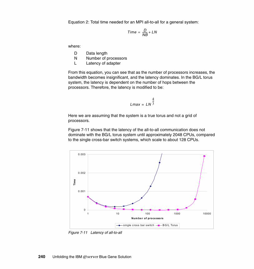
Equation 2: Total time needed for an MPI all-to-all for a general system:

where:

D Data lengthN Number of processorsL Latency of adapter

From this equation, you can see that as the number of processors increases, the bandwidth becomes insignificant, and the latency dominates. In the BG/L torus system, the latency is dependent on the number of hops between the processors. Therefore, the latency is modified to be:

Here we are assuming that the system is a true torus and not a grid of processors.

Figure 7-11 shows that the latency of the all-to-all communication does not dominate with the BG/L torus system until approximately 2048 CPUs, compared to the single cross-bar switch systems, which scale to about 128 CPUs.

Figure 7-11 Latency of all-to-all

Time DNB-------- LN+=

Lmax LN

43---

=

0

0.001

0.002

0.003

1 10 100 1000 10000

Num be r of proce ssors

Tim

e

s ingle c ross bar switch B G/L Torus


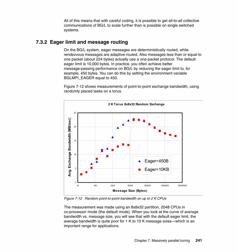
All of this means that with careful coding, it is possible to get all-to-all collective communications of BG/L to scale further than is possible on single switched systems.

7.3.2 Eager limit and message routingOn the BG/L system, eager messages are deterministically routed, while rendezvous messages are adaptive-routed. Also messages less than or equal to one packet (about 224 bytes) actually use a one-packet protocol. The default eager limit is 10,000 bytes. In practice, you often achieve better message-passing performance on BG/L by reducing the eager limit to, for example, 450 bytes. You can do this by setting the environment variable BGLMPI_EAGER equal to 450.

Figure 7-12 shows measurements of point-to-point exchange bandwidth, using randomly placed tasks on a torus.

Figure 7-12 Random point-to-point bandwidth on up to 2 K CPUs

The measurement was made using an 8x8x32 partition, 2048 CPUs in co-processor mode (the default mode). When you look at the curve of average bandwidth vs. message size, you will see that with the default eager limit, the average bandwidth is quite poor for 1 K to 10 K message sizes—which is an important range for applications.

2 K Torus 8x8x32 Random Exchange

0

5

10

15

20

25

10 100 1000 10000 100000 1000000 10000000

Message Size (Bytes)

Avg

. Exc

hang

e B

andw

idth

(MB

/sec

)

Eager=450B

Eager=10KB


Turning the eager limit down to 450 bytes gets adaptive routes working for messages >450 bytes; shorter messages would not benefit, so 450 bytes is generally a good choice.

For a torus, the average number of hops should be torus_size/4 in each dimension. For an 8x8x32 torus, this would be 8 hops in z, 2 hops in x, 2 hops in y; for a total of 12 hops. This should result in an exchange bandwidth that is reduced from the nearest-neighbor value (about 300 MB/sec for medium to large messages) by a factor of 12 => 300/12 = 25 MB/sec. This is reasonably close to the maximum average bandwidth that is measured: about 22.6 MB/sec = 90% of the theoretical bandwidth. Based on Figure 7-12, we think 450 is a good default choice.

7.4 Other general suggestionsThis section is a collection of hints and ideas for scaling applications to large numbers of CPUs.

� Use a torus rather than a grid network.

The CPUs on the torus network are connected via six nearest neighbor links, as shown in Figure 2-4 on page 21. The smallest physical group of nodes that gives a true torus network in three dimensions is 8x8x8 (= 512 nodes). For a group of nodes less than this, the interconnections at the edges are not wrapped around; thus, the network becomes a mesh. Other sizes which are true torus include 16x16x16 (4096) and 32x32x32 (32786) nodes.

For the 8x8x8 torus, the longest random hop length between nodes is given by a quarter of the side length, which in this case is two intermediate node hops away. The worst case for non-nearest neighbor is in a 32x32x64 node torus with two randomly separated nodes by 8+8+16=32 intermediate nodes. A node router takes 12 bytes per link, giving a latency of 32*12 = 384 bytes. This all comes down to flight time of the messages between the nodes.

� Use gather calls on the collective network.

This is done using the appropriate optimized MPI calls listed in 6.3.5, “MPI collective performance” on page 188. The time for the different networks is given in 8.1.4, “Intel MPI Benchmarks” on page 258. From these measurements you can see that it is more efficient to use all reduce type calls using the collective network, rather than using gather type calls.

� In general, for global reductions the all reduce choice is best.

Another reason for using all reduce rather than gather operations is that the single node collecting the gather will quickly run out of memory as the number of nodes is increased.


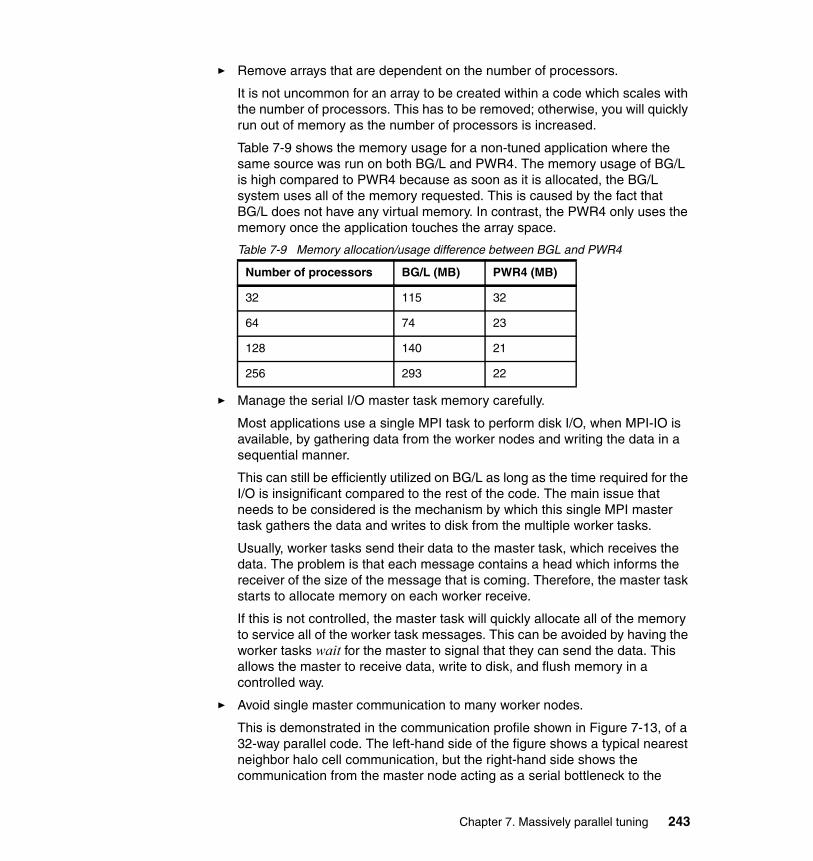
� Remove arrays that are dependent on the number of processors.

It is not uncommon for an array to be created within a code which scales with the number of processors. This has to be removed; otherwise, you will quickly run out of memory as the number of processors is increased.

Table 7-9 shows the memory usage for a non-tuned application where the same source was run on both BG/L and PWR4. The memory usage of BG/L is high compared to PWR4 because as soon as it is allocated, the BG/L system uses all of the memory requested. This is caused by the fact that BG/L does not have any virtual memory. In contrast, the PWR4 only uses the memory once the application touches the array space.

Table 7-9 Memory allocation/usage difference between BGL and PWR4

� Manage the serial I/O master task memory carefully.

Most applications use a single MPI task to perform disk I/O, when MPI-IO is available, by gathering data from the worker nodes and writing the data in a sequential manner.

This can still be efficiently utilized on BG/L as long as the time required for the I/O is insignificant compared to the rest of the code. The main issue that needs to be considered is the mechanism by which this single MPI master task gathers the data and writes to disk from the multiple worker tasks.

Usually, worker tasks send their data to the master task, which receives the data. The problem is that each message contains a head which informs the receiver of the size of the message that is coming. Therefore, the master task starts to allocate memory on each worker receive.

If this is not controlled, the master task will quickly allocate all of the memory to service all of the worker task messages. This can be avoided by having the worker tasks wait for the master to signal that they can send the data. This allows the master to receive data, write to disk, and flush memory in a controlled way.

� Avoid single master communication to many worker nodes.

This is demonstrated in the communication profile shown in Figure 7-13, of a 32-way parallel code. The left-hand side of the figure shows a typical nearest neighbor halo cell communication, but the right-hand side shows the communication from the master node acting as a serial bottleneck to the

Number of processors BG/L (MB) PWR4 (MB)

32 115 32

64 74 23

128 140 21

256 293 22


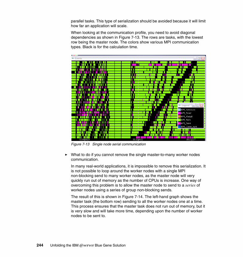
parallel tasks. This type of serialization should be avoided because it will limit how far an application will scale.

When looking at the communication profile, you need to avoid diagonal dependencies as shown in Figure 7-13. The rows are tasks, with the lowest row being the master node. The colors show various MPI communication types. Black is for the calculation time.

Figure 7-13 Single node serial communication

� What to do if you cannot remove the single master-to-many worker nodes communication.

In many real-world applications, it is impossible to remove this serialization. It is not possible to loop around the worker nodes with a single MPI non-blocking send to many worker nodes, as the master node will very quickly run out of memory as the number of CPUs is increase. One way of overcoming this problem is to allow the master node to send to a series of worker nodes using a series of group non-blocking sends.

The result of this is shown in Figure 7-14. The left-hand graph shows the master task (the bottom row) sending to all the worker nodes one at a time. This process ensures that the master task does not run out of memory, but it is very slow and will take more time, depending upon the number of worker nodes to be sent to.


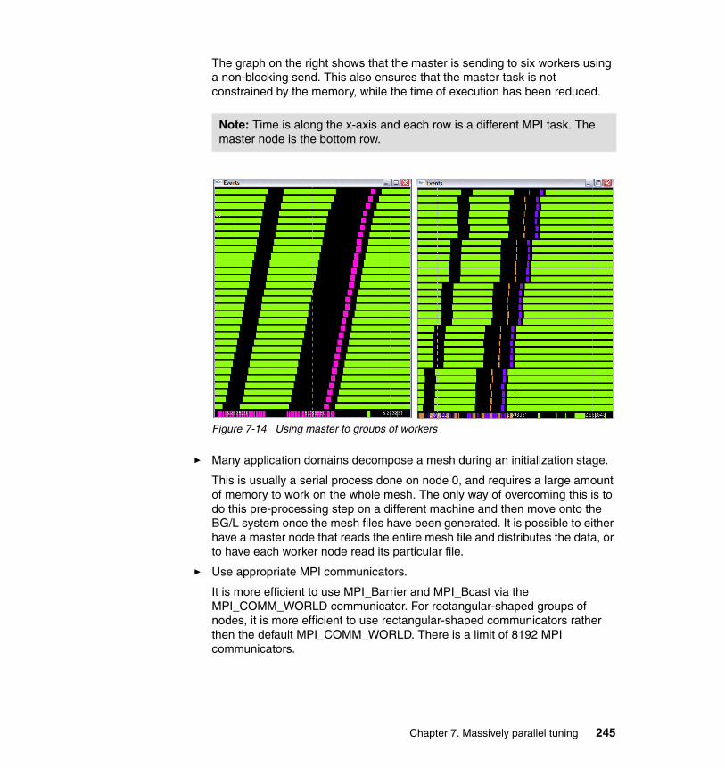
The graph on the right shows that the master is sending to six workers using a non-blocking send. This also ensures that the master task is not constrained by the memory, while the time of execution has been reduced.

Figure 7-14 Using master to groups of workers

� Many application domains decompose a mesh during an initialization stage.

This is usually a serial process done on node 0, and requires a large amount of memory to work on the whole mesh. The only way of overcoming this is to do this pre-processing step on a different machine and then move onto the BG/L system once the mesh files have been generated. It is possible to either have a master node that reads the entire mesh file and distributes the data, or to have each worker node read its particular file.

� Use appropriate MPI communicators.

It is more efficient to use MPI_Barrier and MPI_Bcast via the MPI_COMM_WORLD communicator. For rectangular-shaped groups of nodes, it is more efficient to use rectangular-shaped communicators rather then the default MPI_COMM_WORLD. There is a limit of 8192 MPI communicators.

Note: Time is along the x-axis and each row is a different MPI task. The master node is the bottom row.



Part 3 Application porting examples

This part presents several application porting exercises the redbook team performed during the project. These experiences are presented for reference only, as there is no guarantee if and when the application providers will support their code for running on Blue Gene/L.

The performance data presented for each application was obtained during our tests with minimal optimization of the code. It is the intention in this part to show that it is possible to port applications without initial major effort, and that the success of this porting operation is very much dependent on the application structure and the time allocated for this effort.

Part 3



Chapter 8. Applications on Blue Gene

The first section in this chapter presents some of the results the team that wrote this book obtained running various benchmarks. Since the Blue Gene has a very special architecture, some of the benchmarks may not be suitable to measure performance on this system, thus we have selected for this book only the ones that were possible to port and run in the six weeks allotted for the project.

This chapter also presents experimental results for various applications run on Blue Gene during our six-week project. The applications cover diverse fields (weather, chemistry, and so forth), and have been used as a proof of concept, for demonstration and research purposes only, so there is no warranty or commitment from either IBM or the application owners that these results can be used for commercial purposes.

These applications were ported by either the IBM team or the application provider, or in certain cases, cooperatively by IBM and the application provider.

The examples in this chapter emphasize the benefits of using Blue Gene as a highly scalable parallel system. They present results for running applications in various modes, exploiting the architecture of the system.

8


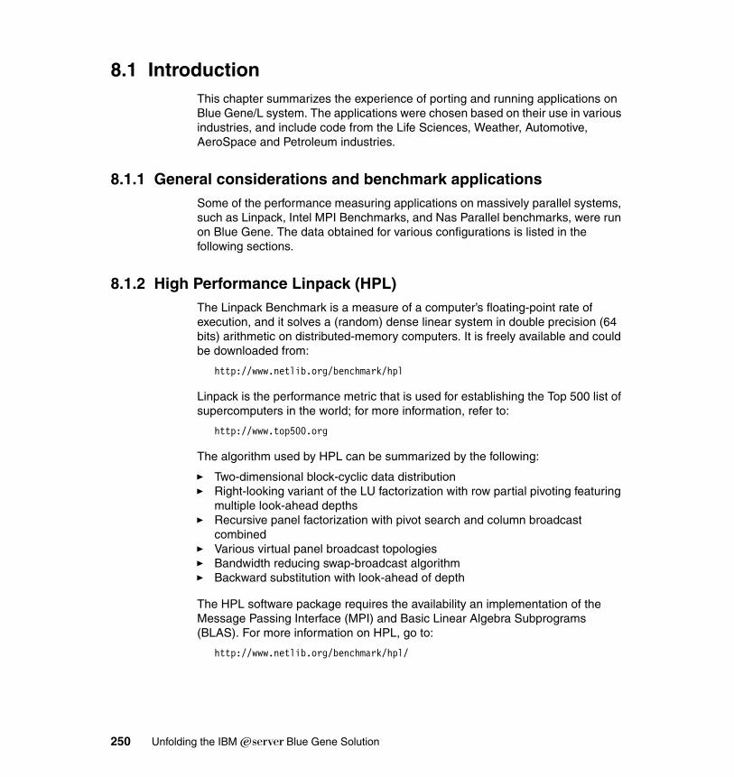
8.1 IntroductionThis chapter summarizes the experience of porting and running applications on Blue Gene/L system. The applications were chosen based on their use in various industries, and include code from the Life Sciences, Weather, Automotive, AeroSpace and Petroleum industries.

8.1.1 General considerations and benchmark applications Some of the performance measuring applications on massively parallel systems, such as Linpack, Intel MPI Benchmarks, and Nas Parallel benchmarks, were run on Blue Gene. The data obtained for various configurations is listed in the following sections.

8.1.2 High Performance Linpack (HPL)The Linpack Benchmark is a measure of a computer’s floating-point rate of execution, and it solves a (random) dense linear system in double precision (64 bits) arithmetic on distributed-memory computers. It is freely available and could be downloaded from:

http://www.netlib.org/benchmark/hpl

Linpack is the performance metric that is used for establishing the Top 500 list of supercomputers in the world; for more information, refer to:

http://www.top500.org

The algorithm used by HPL can be summarized by the following:

� Two-dimensional block-cyclic data distribution� Right-looking variant of the LU factorization with row partial pivoting featuring

multiple look-ahead depths� Recursive panel factorization with pivot search and column broadcast

combined� Various virtual panel broadcast topologies� Bandwidth reducing swap-broadcast algorithm� Backward substitution with look-ahead of depth

The HPL software package requires the availability an implementation of the Message Passing Interface (MPI) and Basic Linear Algebra Subprograms (BLAS). For more information on HPL, go to:

http://www.netlib.org/benchmark/hpl/


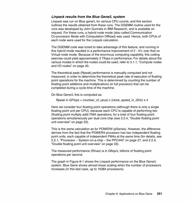
Linpack results from the Blue Gene/L systemLinpack was run on Blue gene/L for various CPU counts, and this section outlines the results obtained from these runs. The DGEMM routine used for the runs was developed by John Gunnels in IBM Research, and is available on request. For these runs, a hybrid node mode (also called Communication Co-processor Mode with Computation Offload) was used. Hence, both CPUs of each node were used for the Linpack calculation.

The DGEMM code was tuned to take advantage of this feature, and running in this hybrid mode resulted in a performance improvement of 2 - 4% over that on Virtual node mode. Because of the enormous computing capability, this coding exercise could yield approximately 3 Tflops in performance. For details about the various modes in which the nodes could be used, refer to 3.1.1, “Compute nodes and I/O nodes” on page 40.

The theoretical peak (Rpeak) performance is manually computed and not measured, in order to determine the theoretical peak rate of execution of floating point operations for the machine. This is determined by counting the number of floating point additions and multiplications (in full precision) that can be completed during a cycle time of the machine.

On Blue Gene/L this is computed as:

Rpeak in GFlops = (number_of_cpus) x (clock_speed_in_GHz) x 4

Here we consider four floating point operations (although there is only a single floating point unit per CPU), because each CPU is capable of performing two (floating point multiply add) FMA operations, for a total of four floating point operations simultaneously per dual core chip (see 2.2.4, “Double floating point unit overview” on page 33).

This is the same calculation as for POWER4 (pSeries). However, the difference derives from the fact that the POWER4 processor has two independent floating point units, each capable of independent FMAs at the same time (for details, see 2.2.1, “Processor – System-on-a-chip – the PPC440” on page 27, and 2.2.4, “Double floating point unit overview” on page 33).

The measured performance (Rmax) is in Gflop/s, billions of floating point operations per second.

The graph in Figure 8-1 shows the Linpack performance on the Blue Gene/L system. Blue Gene shows almost linear scaling when the number of processors increases (in this test case, up to 16384 processors).

Chapter 8. Applications on Blue Gene 251

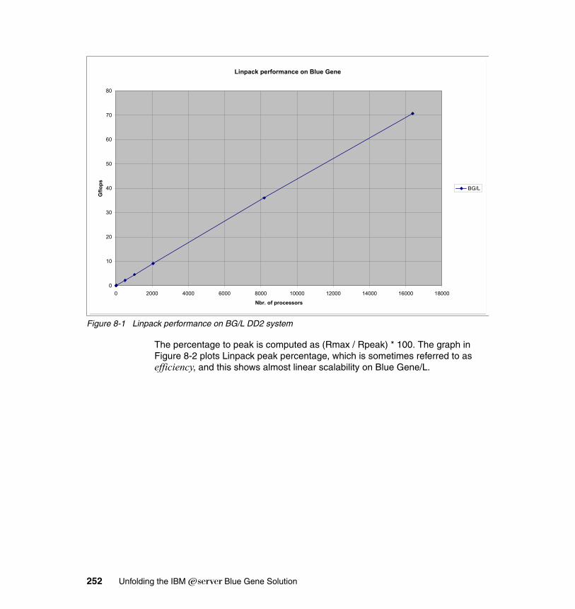
Figure 8-1 Linpack performance on BG/L DD2 system

The percentage to peak is computed as (Rmax / Rpeak) * 100. The graph in Figure 8-2 plots Linpack peak percentage, which is sometimes referred to as efficiency, and this shows almost linear scalability on Blue Gene/L.

Linpack performance on Blue Gene

0

10

20

30

40

50

60

70

80

0 2000 4000 6000 8000 10000 12000 14000 16000 18000

Nbr. of processors

Gflo

ps

BG/L


Figure 8-2 Linpack scalability on BG/L

The Linpack data shown here was received from John Gunnels, IBM Research, at the time of writing.

8.1.3 NAS Parallel BenchmarksThe NAS Parallel Benchmarks (NPB) consist of a small set of programs designed to help evaluate the performance of parallel supercomputers. It has been developed by the National Aeronautics and Space Administration Advanced Supercomputing (NAS) division.

Linpack scalability

60

65

70

75

80

85

90

0 2000 4000 6000 8000 10000 12000 14000 16000 18000

Nbr. of processors

Perc

enta

ge o

f pea

kBG/L

Note: The Linpack benchmark data is changing constantly, as new runs exploit the continuous BG/L software driver and compiler improvements. For more information, refer to:

http://www.top500.org


The benchmarks, which are derived from computational fluid dynamics (CFD) applications, consist of five kernels (FT, MG, IS, EP, CG), and three pseudo-applications (BT, SP, LU). These are MPI-based source-code implementations, written and distributed by NAS. This section presents the benchmark results for FT, MG, CG, and LU.

� The five kernels are:

– EP - Random number generation by the multiplication congruence method

– MG - Simplified multigrid kernel for solving a 3D Poisson PDE

– CG - Conjugate gradient method for finding the smallest eigenvalue of a large-scale sparse symmetric positive definite matrix

– FT - Fast-Fourier transformation for solving a 3D Partial Differential Equation

– IS - Large-scale integer sort

� The three pseudo-applications are:

– LU - CFD application using the symmetric Successive Overrelaxation (SOR) iteration

– SP - CFD application using the scalar Alternating Directions Implicit (ADI) iteration

– BT - CFD application using the 5x5 block size ADI iteration

For details on NAS Parallel Benchmarks, or to download the benchmark suite, see:

http://www.nas.nasa.gov/Software/NPB/

The results from the benchmark execution on two systems are included here. These were performed by San Diego Super Computing Center.

� IBM Eserver Blue Gene Solution, consisting of 2048 700MHz PowerPC 440 compute processors (2-way nodes) connected by various networks

� SDSC DataStar cluster, which has 1440 1.5-GHz Power4+ processors in 8-way p655 nodes connected by a High Performance Switch

On both systems, four NPBs are considered: CG, FT, MG, LU, and all. The test case used was Class C V2.4. Strong scaling scans are presented for each code.

Note: In this discussion “#p” stands for number of processors; for example, 512p stands for 512 processors.


Compiler flags used on Blue Gene/LIn this section, we summarize the experience of using various compiler options on Blue Gene/L:

� The FORTRAN xlf compiler was V9.1.

� Two primary options were considered:

– -O3 -qarch=440d

– -O5 -qarch=440d

� For CG, FT, and MG, -O5 -qarch=440d gave better performance than -O3 -qarch=440d. The speedup is largest (1.14x to 1.17x) for CG on 8p and 16p. The benefit was modest (1.00x to 1.07x) for all three loops on 32p.

� For LU, -O5 -qarch=440d was worse than -O3 -qarch=440d. The slowdown (0.87x to 0.91x) showed little dependence on the number of processors.

� Data with options -O5 -qnoipa -qarch=440d was also measured. This data shows that the speedups for CG and MG, as well as the slowdown for LU, were all due to ipa. The speedup for FT was half due to -O5 and half due to ipa.

� Additional measurements were made for -O3 -qhot=simd -qarch=440d. These results were the same as for -O5 -qarch=440d.

On DataStar (with p655s):� The FORTRAN compiler was V8.1.

� Two primary compiler options were considered:

– -O3 -qarch=pwr4 -qtune=pwr4

– -O4 -qnoipa

� For CG, MG, and LU, performance was essentially the same with either option. The case of MG on 1024p appears worse with -O4 -qnoipa, but this was probably because of noise in the measurement of a very short time.

� For FT, -O4 -qnoipa was better than -O3 -qarch=pwr4 -qtune=pwr4.

The speedup (1.08x to 1.21x) was appreciable for 8p to 512p. For smaller p, the memory bandwidth was not stressed as much. For 1024p, the problem did not scale.

The various plots use the results for the optimal compiler options based on the preceding experience, as shown in Table 8-1.


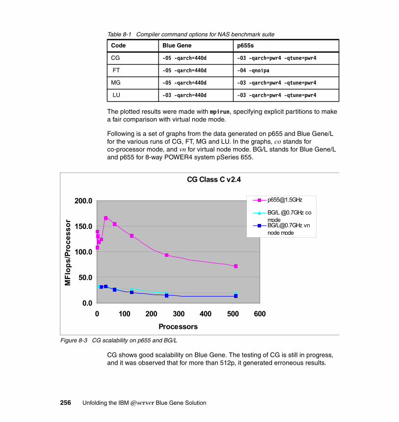
Table 8-1 Compiler command options for NAS benchmark suite

The plotted results were made with mpirun, specifying explicit partitions to make a fair comparison with virtual node mode.

Following is a set of graphs from the data generated on p655 and Blue Gene/L for the various runs of CG, FT, MG and LU. In the graphs, co stands for co-processor mode, and vn for virtual node mode. BG/L stands for Blue Gene/L and p655 for 8-way POWER4 system pSeries 655.

Figure 8-3 CG scalability on p655 and BG/L

CG shows good scalability on Blue Gene. The testing of CG is still in progress, and it was observed that for more than 512p, it generated erroneous results.

Code Blue Gene p655s

CG -O5 -qarch=440d -O3 -qarch=pwr4 -qtune=pwr4

FT -O5 -qarch=440d -O4 -qnoipa

MG -O5 -qarch=440d -O3 -qarch=pwr4 -qtune=pwr4

LU -O3 -qarch=440d -O3 -qarch=pwr4 -qtune=pwr4

CG Class C v2.4

0.0

50.0

100.0

150.0

200.0

0 100 200 300 400 500 600Processors

MFl

ops/

Proc

esso

r

[email protected]

BG/L @0.7GHz comodeBG/[email protected] vnnode mode


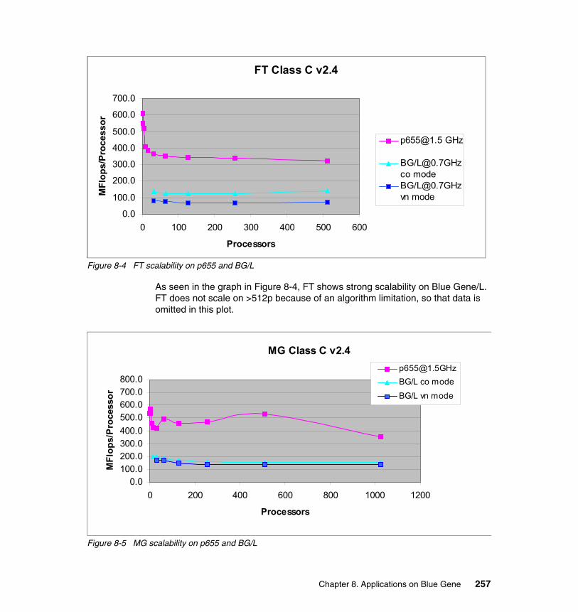
Figure 8-4 FT scalability on p655 and BG/L

As seen in the graph in Figure 8-4, FT shows strong scalability on Blue Gene/L. FT does not scale on >512p because of an algorithm limitation, so that data is omitted in this plot.

Figure 8-5 MG scalability on p655 and BG/L

FT Class C v2.4

0.0

100.0

200.0

300.0

400.0

500.0

600.0

700.0

0 100 200 300 400 500 600

Processors

MFl

ops/

Proc

esso

r

[email protected] GHz

BG/[email protected] modeBG/[email protected] mode

MG Class C v2.4

0.0100.0200.0300.0400.0500.0600.0700.0800.0

0 200 400 600 800 1000 1200

Processors

MFl

ops/

Proc

esso

r

[email protected]/L co mode

BG/L vn mode


The graph in Figure 8-5 shows strong scalability for MG.

Figure 8-6 LU scalability on p655 and BG/L

The graph in Figure 8-6 shows strong scalability for LU on Blue Gene/L.

8.1.4 Intel MPI BenchmarksIntel MPI Benchmarks is formerly known as “Pallas MPI Benchmarks” - PMB-MPI1 (for MPI1 standard functions only).

Intel MPI Benchmarks - MPI1 provides a set of elementary MPI benchmark kernels. You can run all of the supported benchmarks, or just a subset, specified via the command line, can be run. The rules (such as time measurement, message lengths, selection of communicators to run a particular benchmark) are program parameters. For more detail, see the product documentation included in the package downloadable from:

http://www.intel.com/software/products/cluster/mpi/mpi_benchmarks_lic.htm

To help compare the performance of various computing platforms or MPI implementations, the need for a set of well-defined MPI benchmarks arises. This is where Intel MPI Benchmarks (a comprehensive set of MPI benchmarks) comes into play. Its objectives are:

LU Class C v2.4

0.0

500.0

1000.0

1500.0

2000.0

0 200 400 600 800 1000 1200

Processors

MFl

ops/

Proc

esso

[email protected]/L cp mode

BG/L vn mode


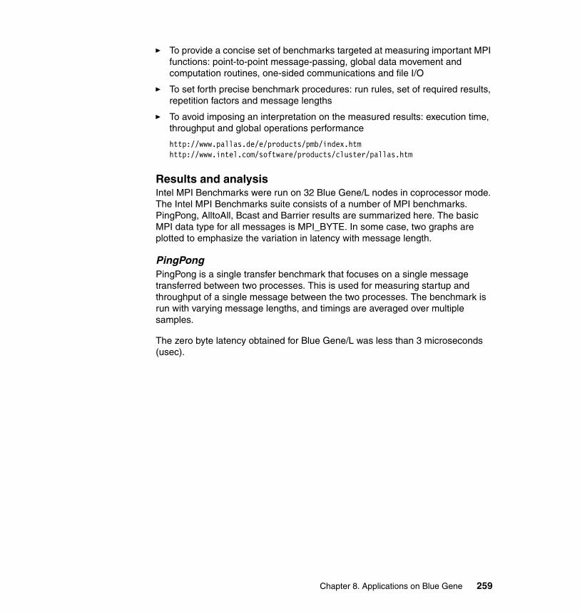
� To provide a concise set of benchmarks targeted at measuring important MPI functions: point-to-point message-passing, global data movement and computation routines, one-sided communications and file I/O

� To set forth precise benchmark procedures: run rules, set of required results, repetition factors and message lengths

� To avoid imposing an interpretation on the measured results: execution time, throughput and global operations performance

http://www.pallas.de/e/products/pmb/index.htmhttp://www.intel.com/software/products/cluster/pallas.htm

Results and analysisIntel MPI Benchmarks were run on 32 Blue Gene/L nodes in coprocessor mode. The Intel MPI Benchmarks suite consists of a number of MPI benchmarks. PingPong, AlltoAll, Bcast and Barrier results are summarized here. The basic MPI data type for all messages is MPI_BYTE. In some case, two graphs are plotted to emphasize the variation in latency with message length.

PingPongPingPong is a single transfer benchmark that focuses on a single message transferred between two processes. This is used for measuring startup and throughput of a single message between the two processes. The benchmark is run with varying message lengths, and timings are averaged over multiple samples.

The zero byte latency obtained for Blue Gene/L was less than 3 microseconds (usec).


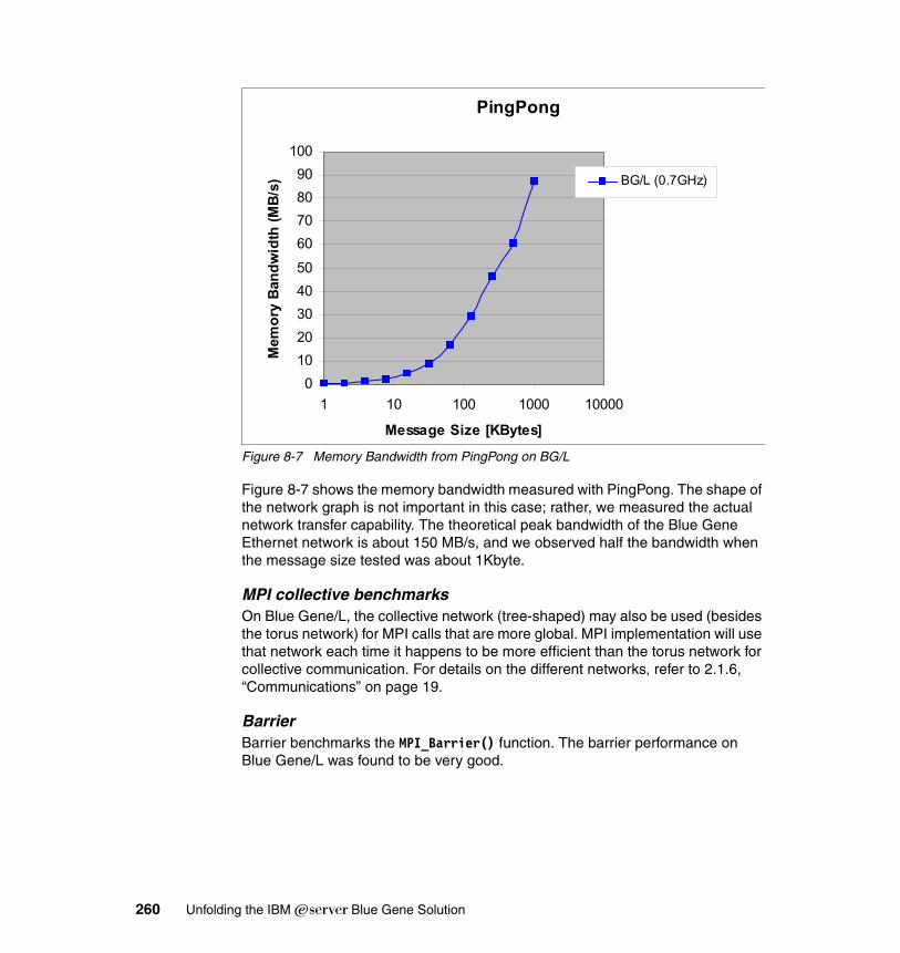
Figure 8-7 Memory Bandwidth from PingPong on BG/L

Figure 8-7 shows the memory bandwidth measured with PingPong. The shape of the network graph is not important in this case; rather, we measured the actual network transfer capability. The theoretical peak bandwidth of the Blue Gene Ethernet network is about 150 MB/s, and we observed half the bandwidth when the message size tested was about 1Kbyte.

MPI collective benchmarksOn Blue Gene/L, the collective network (tree-shaped) may also be used (besides the torus network) for MPI calls that are more global. MPI implementation will use that network each time it happens to be more efficient than the torus network for collective communication. For details on the different networks, refer to 2.1.6, “Communications” on page 19.

BarrierBarrier benchmarks the MPI_Barrier() function. The barrier performance on Blue Gene/L was found to be very good.

PingPong

01020304050

60708090

100

1 10 100 1000 10000

Message Size [KBytes]

Mem

ory

Ban

dwid

th (M

B/s) BG/L (0.7GHz)


Figure 8-8 Barrier BG/L versus p690

In the case of the barrier performance measured on Blue Gene, initially the time increases with the number of processes for 8 processes, then it decreases again at 32 processes. This variation in the barrier performance may be attributed to the way in which the processors are assigned, and the various networking topology that is being used (depending on the number of processors).

For efficiency, Blue Gene has a dedicated (hardware) barrier network, also known as a global interrupt network, and this may be the reason for the very low latency that was observed for the barrier test – for 32 processors it is only 2.75 usec.

The shape of the graph is unexpected, and this is due to the fact that different network algorithms are used for different numbers of processors (we ran the test for 2, 4, 8, 16, and 32 CPUs).

For example, for 8 processors, the intercommunication network shape is 2x2x2 mesh, resulting in an additional layer of communication. Hence, the latency goes up (the global interrupt network does not provide communication to all nodes). This is also the case with the 16 processor run. In the case of 32 processors, however, the dedicated (barrier) hardware takes over the communication, resulting in lower latency.

Barrier

3.49 3.6

4.35

2.752.51

00.5

11.5

22.5

33.5

44.5

5

1 10 100

Number of processors

t_av

g [u

sec]

BG/L @0.7GHz


8.2 DL_POLYDL_POLY is a parallel molecular dynamics (MD) simulation package developed at Daresbury Laboratory UK by W. Smith under auspices of the Engineering and Physical Sciences Research Council (EPSRC) for the EPSRC's Collaborative Computational Project for the Computer Simulation of Condensed Phases and the Molecular Simulation Group at Daresbury Laboratory.

There are two versions of DL_POLY currently available. DL_POLY v2.15 is the original version, which has been parallelized using the Replicated Data strategy and is useful for simulations of up to 30,000 atoms on 100 processors.

DL_POLY v3.02 is a version which uses Domain Decomposition (DD) to achieve parallelism and is suitable for simulations of order 1 million atoms on 8-1024 processors. Both of these versions use distributed data. Because of its suitability for reaching large numbers of CPUs, we concentrate on v3.05 for the following work.

8.2.1 Application descriptionThe DD strategy is one of several ways to achieve parallelization in MD. Its name derives from the division of the simulated system into spatial blocks or domains, each of which is allocated to a specific processor of a parallel compute. The DD strategy underpinning DL_POLY v3 is based on the link cell algorithm of Hockney and Eastwood (ref. Hockney, R. W., and Eastwood, J. W. 1981, Computer Simulation Using Particles. McGraw-Hill International).

This requires that the cut off applied to the interatomic potentials is relatively short-ranged. As with all DD algorithms, there is a need for the processors to exchange halo data, which in the context of link-cells means sending the contents of the link cells at the boundaries of each domain to the neighboring processors so that each may have all necessary information to compute the pair forces acting on the atoms belonging to its allotted domain.The DD strategy is applied to complex molecular systems as follows:

1. Using the atomic coordinates, each processor calculates the forces acting between the atoms in its domain - this requires additional information in the form of the halo data, which must be passed from the neighboring processors beforehand. The forces are usually comprised of:

a. Atom-atom pair forces (for example, Lennard Jones, Coulombic, and so forth)

b. Non-rigid atom-atom bonds

c. Valence angle forces


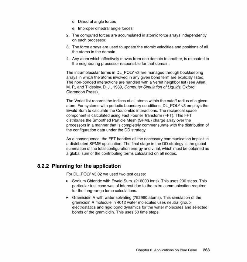
d. Dihedral angle forces

e. Improper dihedral angle forces

2. The computed forces are accumulated in atomic force arrays independently on each processor.

3. The force arrays are used to update the atomic velocities and positions of all the atoms in the domain.

4. Any atom which effectively moves from one domain to another, is relocated to the neighboring processor responsible for that domain.

The intramolecular terms in DL_POLY v3 are managed through bookkeeping arrays in which the atoms involved in any given bond term are explicitly listed. The non-bonded interactions are handled with a Verlet neighbor list (see Allen, M. P., and Tildesley, D. J., 1989, Computer Simulation of Liquids. Oxford: Clarendon Press).

The Verlet list records the indices of all atoms within the cutoff radius of a given atom. For systems with periodic boundary conditions, DL_POLY v3 employs the Ewald Sum to calculate the Coulombic interactions. The reciprocal space component is calculated using Fast Fourier Transform (FFT). This FFT distributes the Smoothed Particle Mesh (SPME) charge array over the processors in a manner that is completely commensurate with the distribution of the configuration data under the DD strategy.

As a consequence, the FFT handles all the necessary communication implicit in a distributed SPME application. The final stage in the DD strategy is the global summation of the total configuration energy and virial, which must be obtained as a global sum of the contributing terms calculated on all nodes.

8.2.2 Planning for the applicationFor DL_POLY v3.02 we used two test cases:

� Sodium Chloride with Ewald Sum. (216000 ions). This uses 200 steps. This particular test case was of interest due to the extra communication required for the long-range force calculations.

� Gramicidin A with water solvating (792960 atoms). This simulation of the gramicidin A molecule in 4012 water molecules uses neutral group electrostatics and rigid bond dynamics for the water molecules and selected bonds of the gramicidin. This uses 50 time steps.


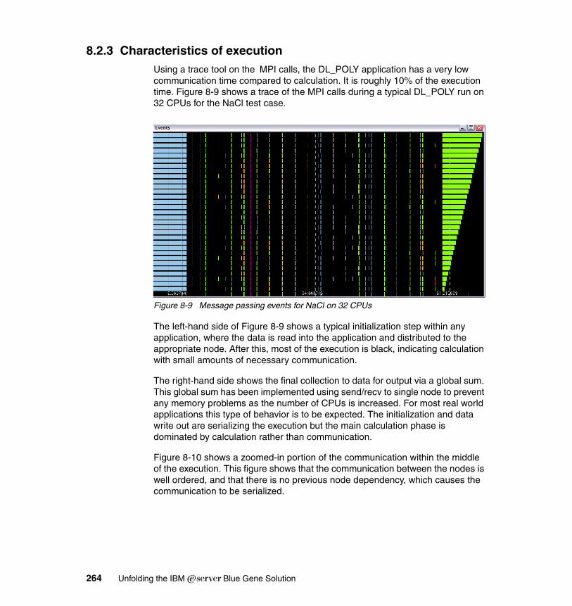
8.2.3 Characteristics of executionUsing a trace tool on the MPI calls, the DL_POLY application has a very low communication time compared to calculation. It is roughly 10% of the execution time. Figure 8-9 shows a trace of the MPI calls during a typical DL_POLY run on 32 CPUs for the NaCl test case.

Figure 8-9 Message passing events for NaCl on 32 CPUs

The left-hand side of Figure 8-9 shows a typical initialization step within any application, where the data is read into the application and distributed to the appropriate node. After this, most of the execution is black, indicating calculation with small amounts of necessary communication.

The right-hand side shows the final collection to data for output via a global sum. This global sum has been implemented using send/recv to single node to prevent any memory problems as the number of CPUs is increased. For most real world applications this type of behavior is to be expected. The initialization and data write out are serializing the execution but the main calculation phase is dominated by calculation rather than communication.

Figure 8-10 shows a zoomed-in portion of the communication within the middle of the execution. This figure shows that the communication between the nodes is well ordered, and that there is no previous node dependency, which causes the communication to be serialized.


Figure 8-10 Communications within central calculation phase (zoomed in)

8.2.4 Scaling and tuning (optimization)The following two graphs, Figure 8-11 and Figure 8-12, show comparative performance for Blue Gene and IBM POWER4 machines. These comparisons are artificial because most test cases for BGL would be large enough to exercise many 1000s of CPUs, but most computer centers do not have POWER4 clusters with more than 1000 CPUs. Consequently, to make a comparison of performance, we have reduced the problem size, which obviously reduces the MMP characteristics of the BGL system. What these tests do show, however, is the parallel scaling of the application, and they hint at the type of input data sets required.


Figure 8-11 NaCl test case on BGL and PWR4

The NaCl test case shows that the BGL system scales very well with increased CPUs, as indicated by the higher gradient. Ideal scaling would be a 45 degree line. The application also behaves well in that there are no obvious serial sections in the execution, as the line is straight. Also, the fact that the lines would pass though the origin shows that the application is not dominated by the serial input or output stage.

NaCl original

0

100

200

300

400

500

600

0 0.005 0.01 0.015 0.02 0.025 0.03 0.035

1/(number of CPUs)

Elap

sed

time

BGL PWR4


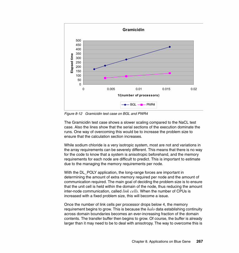
Figure 8-12 Gramicidin test case on BGL and PWR4

The Gramicidin test case shows a slower scaling compared to the NaCL test case. Also the lines show that the serial sections of the execution dominate the runs. One way of overcoming this would be to increase the problem size to ensure that the calculation section increases.

While sodium chloride is a very isotropic system, most are not and variations in the array requirements can be severely different. This means that there is no way for the code to know that a system is anisotropic beforehand, and the memory requirements for each node are difficult to predict. This is important to estimate due to the managing the memory requirements per node.

With the DL_POLY application, the long-range forces are important in determining the amount of extra memory required per node and the amount of communication required. The main goal of deciding the problem size is to ensure that the unit cell is held within the domain of the node, thus reducing the amount inter-node communication, called link cells. When the number of CPUs is increased with a fixed problem size, this will become a issue.

Once the number of link cells per processor drops below 4, the memory requirement begins to grow. This is because the halo data establishing continuity across domain boundaries becomes an ever-increasing fraction of the domain contents. The transfer buffer then begins to grow. Of course, the buffer is already larger than it may need to be to deal with anisotropy. The way to overcome this is

Gramicidin

050

100150200250300350400450500

0 0.005 0.01 0.015 0.02

1/(number of processors)

Elap

sed

time

BGL PWR4


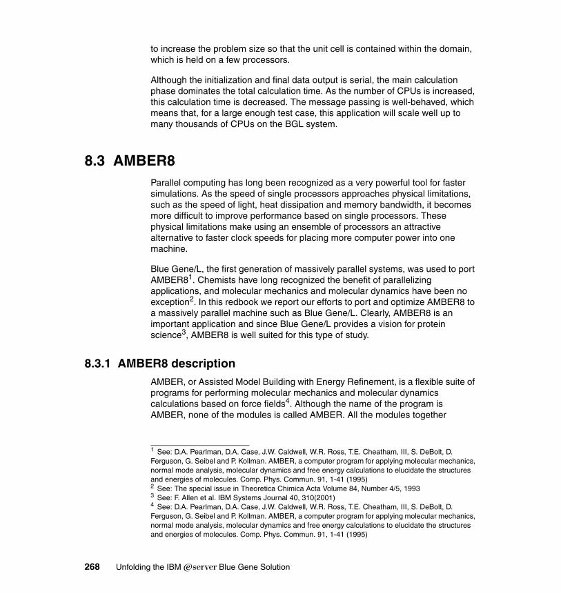
to increase the problem size so that the unit cell is contained within the domain, which is held on a few processors.

Although the initialization and final data output is serial, the main calculation phase dominates the total calculation time. As the number of CPUs is increased, this calculation time is decreased. The message passing is well-behaved, which means that, for a large enough test case, this application will scale well up to many thousands of CPUs on the BGL system.

8.3 AMBER8Parallel computing has long been recognized as a very powerful tool for faster simulations. As the speed of single processors approaches physical limitations, such as the speed of light, heat dissipation and memory bandwidth, it becomes more difficult to improve performance based on single processors. These physical limitations make using an ensemble of processors an attractive alternative to faster clock speeds for placing more computer power into one machine.

Blue Gene/L, the first generation of massively parallel systems, was used to port AMBER81. Chemists have long recognized the benefit of parallelizing applications, and molecular mechanics and molecular dynamics have been no exception2. In this redbook we report our efforts to port and optimize AMBER8 to a massively parallel machine such as Blue Gene/L. Clearly, AMBER8 is an important application and since Blue Gene/L provides a vision for protein science3, AMBER8 is well suited for this type of study.

8.3.1 AMBER8 descriptionAMBER, or Assisted Model Building with Energy Refinement, is a flexible suite of programs for performing molecular mechanics and molecular dynamics calculations based on force fields4. Although the name of the program is AMBER, none of the modules is called AMBER. All the modules together

1 See: D.A. Pearlman, D.A. Case, J.W. Caldwell, W.R. Ross, T.E. Cheatham, III, S. DeBolt, D. Ferguson, G. Seibel and P. Kollman. AMBER, a computer program for applying molecular mechanics, normal mode analysis, molecular dynamics and free energy calculations to elucidate the structures and energies of molecules. Comp. Phys. Commun. 91, 1-41 (1995) 2 See: The special issue in Theoretica Chimica Acta Volume 84, Number 4/5, 19933 See: F. Allen et al. IBM Systems Journal 40, 310(2001)4 See: D.A. Pearlman, D.A. Case, J.W. Caldwell, W.R. Ross, T.E. Cheatham, III, S. DeBolt, D. Ferguson, G. Seibel and P. Kollman. AMBER, a computer program for applying molecular mechanics, normal mode analysis, molecular dynamics and free energy calculations to elucidate the structures and energies of molecules. Comp. Phys. Commun. 91, 1-41 (1995)


perform different functions and collectively are used to simulate large biomolecular systems.

To provide a brief overview as to how AMBER works, Figure 8-13 illustrates schematically how data flows from the initial set of Cartesian coordinates to the energy programs and finally to the analysis of the results. The set of Cartesian coordinates correspond to each of the atoms in the entire systems; they are usually obtained from x-ray crystallography, NMR spectroscopy, or by using a graphical friendly interface to build the actual system of interest. The input for the Cartesian coordinates is required in the Protein Databank (PDB™) format.

Figure 8-13 Selected modules and data flow in AMBER

The programs LEaP and Antechamber provide utilities or functionality to prepare all the files that are required to run the energy programs. The other files required to run the energy program correspond to the topology files that contain information about connectivity, atom names, atom types, residue names, and charges. Information for standard parameters is also available. Finally, another important file contains all the commands; this file is normally called mdin or gbin, depending on the type of calculation.

Antechamber, LEaP

Cartesian coordinates

for each atom in the system (

PDB format)

LES Information

Sander, nmode, pmemd

NMR or XRAY

Information mm-pbsa ptraj

prmtop prmcrd


8.3.2 AMBER8 characteristicsWithin AMBER8, Sander is the primary program used for molecular dynamics simulations, and is the only program considered in our current study. Sander carries out energy minimization, molecular dynamics, and NMR refinements. AMBER is floating point-intensive FORTRAN code. Sander performs minimizations and molecular dynamics. The minimization of the energy is fairly standard and involves changes in the structure to lower the energy of the system until a sufficiently low gradient is found.

On the other hand, the molecular dynamics of the code carry out simulations by integrating Newtonian equations of motion. The MD calculations save system configurations at regular intervals during the simulation. This is done sequentially and it is used for analysis. Basic free energy calculations using thermodynamics integration can also be performed. The version used in this study corresponds to AMBER8 for IBM systems. For more information about AMBER on IBM systems, visit:

http://www.msi.umn.edu/~cpsosa/ChemApps/MolMech/amber/amber.html

The initial version utilized to port Sander was mainly the IBM AIX version. However, since it was also running on Linux on POWER, sections of this version were used as well. Since there is an AIX version and Linux on POWER as well, porting AMBER8 was not difficult. AMBER8 uses MPI for message passing. Most of the work was in transforming the AIX configure file into a Blue Gene/L file.

8.3.3 Planning for AMBER8 AMBER8 has been installed and tested on a number of platforms, using UNIX machines from IBM, Sun™, Hewlett-Packard, DEC (Compaq), and Silicon Graphics, and on Red Hat Linux and Windows 95/98/NT/2000 (running on Intel Pentium and Itanium® machines).

The AMBER8 programs mainly utilize dynamic memory allocation, and do not need to be compiled for any specific size of problem. Some sizes related to NMR refinements are defined in nmr.h, and some dimensioning information for QM/MM calculations is in cp.h. If you receive error messages directing you to look at these files, you may need to edit them, then recompile.

The current Blue Gene/L version of AMBER8 targets sander and pmemd to run on the compute nodes. All the other modules will have to be run on the front-end node. This is due to the fact that sander and pmemd are the most CPU-intensive modules and the ones that have extensively been parallelized.


http://www.msi.umn.edu/~cpsosa/ChemApps/MolMech/amber/amber.html

8.3.4 Blue Gene/L featuresThe system used to carry out this study was an early release of Blue Gene/L prototype hardware consisting of 4096 nodes. Each node has 256 MB of memory. Each node is has two PowerPC 440 cores (a low-power processor typically used in embedded applications). Each node has 4 MB of L3 cache shared between the two cores.

Each core has a small L2 cache that is coherent between the two cores, and a larger L1 (32 K instruction and 32 K data) that is not coherent. Each node has five networks, three of which are available to user applications. These networks are:

� A 3D point-to-point torus running at 1.25 Gb/sec per link on each of the six links.

� A global interrupt network used for extremely fast barriers.

� A global collective (tree) that can be used for reductions, broadcasts, and barriers. The collective network has a 2.5 Gb/sec bandwidth.

The actual production Blue Gene/L system consists of 16384 nodes (32768 processors). Each node has 512 MB of memory. The nodes are the same as the prototype hardware, except that the clocks run at 700 MHz. Because everything in the node is on the same ASIC, the 40% increase in clock frequency usually results in more than a 40% improvement in performance because the memory is faster and the networks are faster (1.4Gb/sec on each of the 6 links on the torus. 2.8Gb/s on the tree). All the runs were carried out using the co-processor mode.

Both machines are located at IBM in Rochester, Minnesota. The early prototype system is #8 on the top500 supercomputers list. The 16-rack system in Rochester is currently the fastest machine in the world.

8.3.5 Scaling and tuning AMBER8 It is important to point out that the study presented here corresponds to Part I. In Part I, our objective is to port AMBER8 to Blue Gene/L and test a series of input files to evaluate the scalability. Part II looks at optimizing AMBER8 for the Blue Gene/L architecture (scalability) as well as for the PowerPC 700 MHz architecture (single processor performance). Thus, in Part I we used a prototype machine for most of our runs. The objective was to look at the porting experience and identify the cases that tend to scale well on this type of architecture.

The first test that we selected to run AMBER is the jac benchmark; see Figure 8-14. This is a joint AMBER-CHARMM benchmark. It considers a protein dhfr (dihydrofolate reductase) in an explicit water bath with cubic periodic boundary conditions. Details of system size and simulation conditions are 23,558


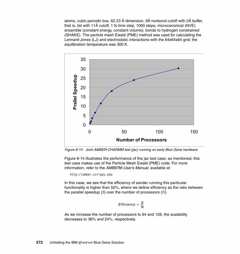
atoms, cubic periodic box, 62.23 Å dimension, 9Å nonbond cutoff with 2Å buffer, that is, list with 11Å cutoff, 1 fs time step, 1000 steps, microcanonical (NVE) ensemble (constant energy, constant volume), bonds to hydrogen constrained (SHAKE). The particle mesh Ewald (PME) method was used for calculating the Lennard-Jones (LJ) and electrostatic interactions with the 64x64x64 grid; the equilibration temperature was 300 K.

Figure 8-14 Joint AMBER-CHARMM test (jac) running on early Blue Gene hardware

Figure 8-14 illustrates the performance of the jac test case; as mentioned, this test case makes use of the Particle Mesh Ewald (PME) code. For more information, refer to the AMBER8 User’s Manual, available at:

http://amber.scripps.edu

In this case, we see that the efficiency of sander running this particular functionality is higher than 50%, where we define efficiency as the ratio between the parallel speedup (S) over the number of processors (N).

As we increase the number of processors to 64 and 128, the scalability decreases to 38% and 24%, respectively.

0

5

10

15

20

25

30

35

0 50 100 150

Number of Processors

Pral

lel S

peed

up

Efficiency SN----=


Example 8-1 illustrates where most of the time is spent when running the PME option in the sander module. This MPI profile is fairly different from the one that we illustrate for the generalized Born functionality.

Example 8-1 The jac profile capture on processor 127

>>>>>>>>PROFILE of TIMES for process 127 Build the list 3.42 (69.82% of List ) Other 1.48 (30.18% of List ) List time 4.90 ( 8.62% of Nonbo) Short_ene time 14.65 (63.32% of Direc) Other 8.49 (36.68% of Direc) Direct Ewald time 23.14 (44.55% of Ewald) Adjust Ewald time 0.16 ( 0.31% of Ewald) Self Ewald time 0.01 ( 0.02% of Ewald) Fill Bspline coeffs 5.49 (27.57% of Recip) Fill charge grid 0.22 ( 1.08% of Recip) Scalar sum 0.01 ( 0.05% of Recip) Grad sum 0.36 ( 1.79% of Recip) FFT communication ti 5.82 (50.19% of FFT t) Other 5.78 (49.81% of FFT t) FFT time 11.60 (58.32% of Recip) Other 2.23 (11.19% of Recip) Recip Ewald time 19.89 (38.30% of Ewald) Force Adjust 3.39 ( 6.52% of Ewald) Virial junk 5.02 ( 9.66% of Ewald) Start sycnronization 0.29 ( 0.56% of Ewald) Other 0.04 ( 0.08% of Ewald) Ewald time 51.95 (91.36% of Nonbo) Other 0.01 ( 0.02% of Nonbo) Nonbond force 56.86 (79.76% of Force) Bond/Angle/Dihedral 1.15 ( 1.61% of Force) FRC Collect time 12.96 (18.18% of Force) Other 0.32 ( 0.45% of Force) Force time 71.28 (86.30% of Runmd) Shake time 0.90 ( 1.09% of Runmd) Verlet update time 1.39 ( 1.68% of Runmd) CRD distribute time 8.98 (10.87% of Runmd) Other 0.05 ( 0.06% of Runmd) Runmd Time 82.60 (96.42% of Total) Other 3.07 ( 3.58% of Total) Total time 85.67 (100.0% of ALL )

The second test corresponds to a generalized Born myoglobin simulation. This protein has 2492 atoms, and is run with a 20 Å cutoff and a salt concentration of 0.2 M, with nrespa=4 (long-range forces computed every 4 steps). This is the test case in the benchmarks/gb_mb subdirectory of the AMBER8 distribution.


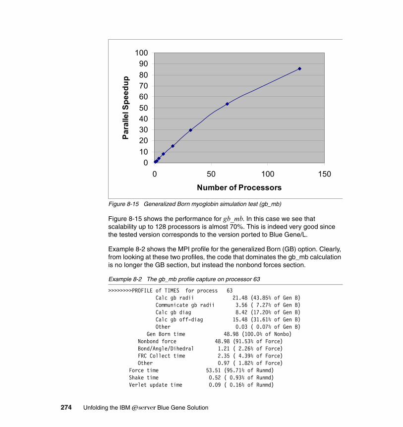
Figure 8-15 Generalized Born myoglobin simulation test (gb_mb)

Figure 8-15 shows the performance for gb_mb. In this case we see that scalability up to 128 processors is almost 70%. This is indeed very good since the tested version corresponds to the version ported to Blue Gene/L.

Example 8-2 shows the MPI profile for the generalized Born (GB) option. Clearly, from looking at these two profiles, the code that dominates the gb_mb calculation is no longer the GB section, but instead the nonbond forces section.

Example 8-2 The gb_mb profile capture on processor 63

>>>>>>>>PROFILE of TIMES for process 63 Calc gb radii 21.48 (43.85% of Gen B) Communicate gb radii 3.56 ( 7.27% of Gen B) Calc gb diag 8.42 (17.20% of Gen B) Calc gb off-diag 15.48 (31.61% of Gen B) Other 0.03 ( 0.07% of Gen B) Gen Born time 48.98 (100.0% of Nonbo) Nonbond force 48.98 (91.53% of Force) Bond/Angle/Dihedral 1.21 ( 2.26% of Force) FRC Collect time 2.35 ( 4.39% of Force) Other 0.97 ( 1.82% of Force) Force time 53.51 (95.71% of Runmd) Shake time 0.52 ( 0.93% of Runmd) Verlet update time 0.09 ( 0.16% of Runmd)

0102030405060708090

100

0 50 100 150


Para

llel S

peed

up


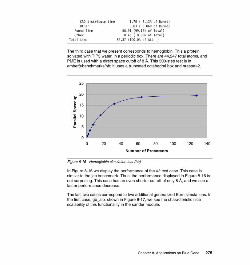
CRD distribute time 1.75 ( 3.13% of Runmd) Other 0.03 ( 0.06% of Runmd) Runmd Time 55.91 (99.18% of Total) Other 0.46 ( 0.82% of Total) Total time 56.37 (100.0% of ALL )

The third case that we present corresponds to hemoglobin. This a protein solvated with TIP3 water, in a periodic box. There are 44,247 total atoms, and PME is used with a direct space cutoff of 8 Å. This 500-step test is in amber8/benchmarks/hb; it uses a truncated octahedral box and nrespa=2.

Figure 8-16 Hemoglobin simulation test (hb)

In Figure 8-16 we display the performance of the hb test case. This case is similar to the jac benchmark. Thus, the performance displayed in Figure 8-16 is not surprising. This case has an even shorter cut-off of only 8 Å, and we see a faster performance decrease.

The last two cases correspond to two additional generalized Born simulations. In the first case, gb_alp, shown in Figure 8-17, we see the characteristic nice scalability of this functionality in the sander module.

0

5

10

15

20

25

0 20 40 60 80 100 120 140


Para

llel S

peed

up


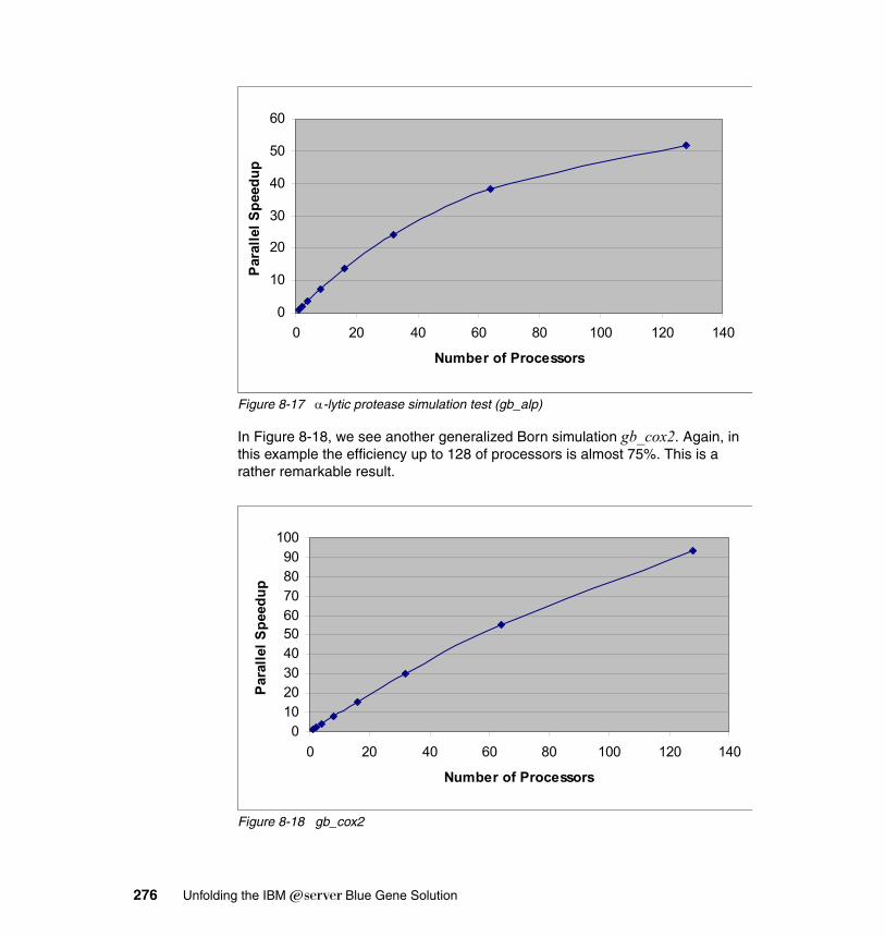
Figure 8-17 α-lytic protease simulation test (gb_alp)

In Figure 8-18, we see another generalized Born simulation gb_cox2. Again, in this example the efficiency up to 128 of processors is almost 75%. This is a rather remarkable result.

Figure 8-18 gb_cox2

0

10

20

30

40

50

60

0 20 40 60 80 100 120 140


Para

llel S

peed

up

0102030405060708090

100

0 20 40 60 80 100 120 140


Para

llel S

peed

up


In summary, we have shown that AMBER8 is a well-suited application for an architecture such as Blue Gene/L. In Part II we look at optimization and further scalability, as well as testing the pmemd module.

8.4 AVBPAVBP is a standard code used in Europe to perform Large Eddy Simulation of reacting flows in complex geometry combustors. The main fields of application are gas turbines, rocket engines, industrial furnaces, and piston engines. This code solves the fully compressible unsteady Navier Stokes equations for laminar and turbulent reacting flows on hybrid grids (Moureau et al., 2005). It was built with European support in the 90s, specifically for parallel computers.

In the last five years, AVBP has started to reach its full potential, allowing computations of both non-reacting (Schluter et al., 2000, 2004, Priere et al., 2004) and reacting flows in complex geometries (Angelberger et al., 2000, Selle et al., 2004). AVBP is developed jointly by CERFACS and Institut Français du Pétrole. It is used by multiple laboratories (EM2C in Paris, IRPHE in Marseille, IMF in Toulouse, Coria in Rouen, University of Belfast, University of Munchen, University of Twente, and others), and is the baseline code for at least 20 PhDs in 2005. It is used for multiple industrial applications by Siemens, Alstom, PSA, Ferrari, SNECMA, Turbomeca, Air Liquide, MBDA, and so forth. It is also installed and used on sites by industrial partners of CERFACS such as MBDA, SNECMA or TURBOMECA.

8.4.1 Application descriptionThe AVBP project started in January 1993 upon an initiative of Michael Rudgyard and Thilo Schönfeld with the goal of building a modern software tool for Computational Fluid Dynamics (CFD) within CERFACS of high flexibility, efficiency, and modularity. Since then, the project has grown rapidly and today AVBP represents one of the most advanced CFD tools in Europe for the numerical simulation of unsteady turbulence for reacting flows. AVBP is widely used both for basic research and applied research of industrial interest. Today, the AVBP project is comprised of a total of approximately 30 research scientists and engineers.

As mentioned, AVBP is a parallel CFD code that solves the laminar and turbulent compressible Navier-Stokes equations in two and three space dimensions on unstructured and hybrid grids. While initially conceived for steady state flows of aerodynamics, today the current exclusive area of applications is the modelling of unsteady (reacting) flows. These activities are strongly related to the rising importance paid to the understanding of the flow structure and mechanisms


leading to turbulence. The prediction of these unsteady turbulent flows is based on the Large Eddy Simulation (LES) approach. An Arrhenius law reduced chemistry model allows investigation of combustion for complex configurations.

The important development of the physical models done at CERFACS was completed by academic studies carried out at the EM2C lab of Ecole Central Paris (ECP) and Institut de Mécanique des Fluids de Toulouse (IMFT). Further significant development has been done at IFP Institut Francais de Pétrole (IFP), located in Rueil-Malmaison near Paris, following an agreement of joint code development oriented towards piston engine applications.

The capability to handle structured, unstructured, or hybrid grids is one key feature of AVBP. With the use of these hybrid grids, where a combination of several elements of different types is used in the framework of the same mesh, the advantages of the structured and unstructured grid methodologies are combined in terms of gridding flexibility and solution accuracy.

In order to handle such arbitrary hybrid grids, the data structure of AVBP employs a cell-vertex finite-volume approximation. The basic numerical methods are based on a Lax-Wendroff or a Finite-Element type low-dissipation Taylor-Galerkin discretization, in combination with a linear-preserving artificial viscosity model.

AVBP is built upon a modular software library of subroutines that aims to free the non-specialist user from the need to consider aspects of high performance computing. A data parallel strategy is used that includes integrated parallel domain partition and data reordering tools, handles message passing and includes supporting routines for dynamic memory allocation, routines for parallel I/O, and iterative methods. AVBP is based on a generalized data structure which is suitable for structured and unstructured meshes of arbitrary elements. AVBP is highly portable to most standard platforms including PCs, workstations and mainframes, and has proven to be efficient on most parallel RISC architectures.

Mesh-related aspects of AVBP are handled by the multi-function grid-preprocessor HIP. This grid manipulation tool allows various operations such as generic solution interpolation between two grids, grid cutting or gluing, grid validation, adaptive local grid refinement, grid extrusion or the creation of axi-symmetric grids.

The AVBP solver is utilized in the frame of many bilateral industrial collaborations and national research programs (such as the supersonic COS program and the joint research and development initiative PRC SNECMA ONERA). On a European level, AVBP is used in several programs of the running 5th Framework Program of the EC:

– PRECCINSTA on low NOx studies for gas turbines


– STOPP network on chemistry – MOLECULES– DESIRE on gas turbine flows and fluid/structure interaction in liners – FUELCHIEF on fuel-staged combustion instabilities– LESSCO2 for piston engines– In the frame of FP6, AVBP is used in the INTELLECT-DM project

AVBP is used by members of the CFD team flow simulations in the frame of the demanding summer school program at the Center for Turbulence Research at Stanford University.

Finally, a hands-on course in MCIP based on AVBP is given for final year undergraduate students with specialization in CFD in the frame of the series Mastering of Industrial Codes and Parallelism at the ENSEEIHT engineering school of the INPT Technical University in Toulouse.

References:

Moureau, V., Lartigue, G., Sommerer, Y., Angelberger, C., Colin, O. and Poinsot, T. High-order methods for DNS and LES of compressible multi-component reacting flows on fixed and moving grids. J. Comp. Phys. 202, 710-736 (2005).

Faivre, V. and T. Poinsot "Experimental and numerical investigations of jet active control for combustion applications." J. of Turb. 5: 025 (2004).

Selle, L., Lartigue, G., Poinsot, T., Koch, R., Schildmacher, K.-U., Krebs, W., Prade, B., Kaufmann, P. et Veynante, D. ''Compressible Large-Eddy Simulation of turbulent combustion in complex geometry on unstructured meshes''. Comb. Flame, 137, 489-505 (2004).

Prière, C., Gicquel, L., Kaufmann, P. Krebs, W. et Poinsot T. ''Predictions of mixing enhancement for jets in Cross Flows '' J. of Turb. 5, 1, 30 (2004).

C. Angelberger, D. Veynante, and F. Egolfopoulos. Large Eddy Simulations of chemical and acoustic forcing of a premixed dump combustor. Flow, Turbulence and Combustion, 65(2):205-222, 2000.

J. Schlüter and T. Schönfeld. LES of jets in cross flow and its application to gas turbine burners. Flow, Turbulence and Combustion, 65(2):177-203, 2000.

J. Schlüter. Axi-symmetric and full 3D LES of swirl flows. International Journal of Computational Fluid Dynamics, 18(3):235-246, 2004.

For more information on AVBP, see:

http://www.cerfacs.fr/cfd/avbp_code.php


8.4.2 Planning for the applicationAVBP is already running on quite a few platforms and its scalability has largely been proven. The idea behind porting it to Blue Gene/L was to look for a very large number of processors. Blue Gene/L can have up to 64 K nodes (131072 processors), but in the brief time we had for this project, cutting the mesh in a load-balanced way limited the experience to 5000 nodes.

A first test case was chosen because it could be compared to previous experiences going from 16 nodes to 768 nodes. Then a larger test case was run from 512 to 5120 nodes.

8.4.3 Porting experienceAVBP had already been ported to pSeries Linux. We only had to enter the proper compiler names and options and the proper libraries to port AVBP to Blue Gene/L.

The only difficulty we encountered was the node memory size. Blue Gene/L nodes have 512 MB of memory, and in some cases applications need more than that. There is not enough memory to do the grid partitioning, so this was achieved on some other machine (like the front-end ndeo), and the results used as input files for the different test cases.

Because Blue Gene/L can have so many nodes and is so densely packaged, you can compensate for the small memory size by using a larger number of nodes. For example, the first test case needed at least 16 nodes to run in coprocessor mode, because on a smaller number of nodes it needs more than 512 MB. In virtual node mode at least 64 processors are needed, since each one only has 256 MB of memory.

8.4.4 Scaling and tuningGetting the data to the nodes at the beginning of each run actually takes more and more time as the number of nodes is increased. The same issue occurs at the end of the run (for collecting data). We provide the MPI trace so you can see that the operations are serialized; task zero exchanges data with all other tasks, but one at a time. This only happens once in the job, as opposed to the numerous iterations (tens of thousands), that represent the main part of the code. Therefore, you do not spend much time optimizing it. The scaling of the application shown in Figure 8-19 is computed on the iterative part of the code.

Blue Gene/L can work in two modes: coprocessor mode, and virtual node mode. With AVBP, the virtual node mode worked quite efficiently, only 1.1 times slower than the coprocessor mode, even though it used half the number of nodes.


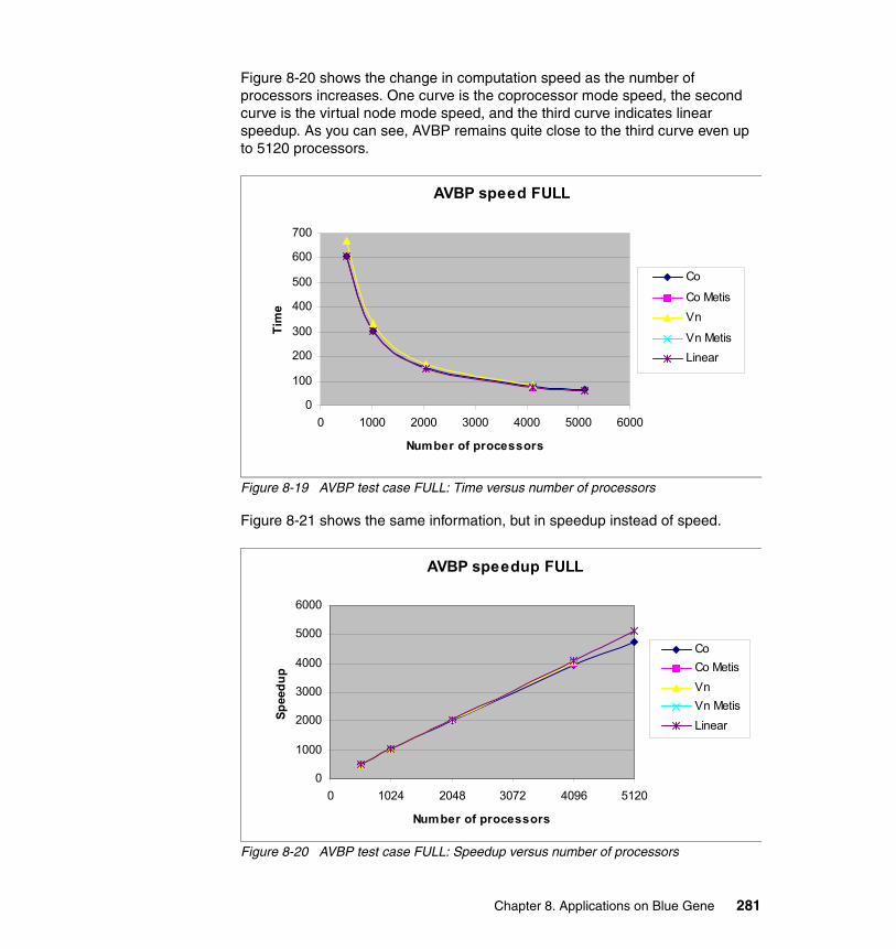
Figure 8-20 shows the change in computation speed as the number of processors increases. One curve is the coprocessor mode speed, the second curve is the virtual node mode speed, and the third curve indicates linear speedup. As you can see, AVBP remains quite close to the third curve even up to 5120 processors.

Figure 8-19 AVBP test case FULL: Time versus number of processors

Figure 8-21 shows the same information, but in speedup instead of speed.

Figure 8-20 AVBP test case FULL: Speedup versus number of processors

AVBP speed FULL

0

100

200

300

400

500

600

700

0 1000 2000 3000 4000 5000 6000


Tim

eCo

Co MetisVn

Vn MetisLinear

AVBP speedup FULL

0

1000

2000

3000

4000

5000

6000

0 1024 2048 3072 4096 5120


Spee

dup

CoCo MetisVnVn MetisLinear


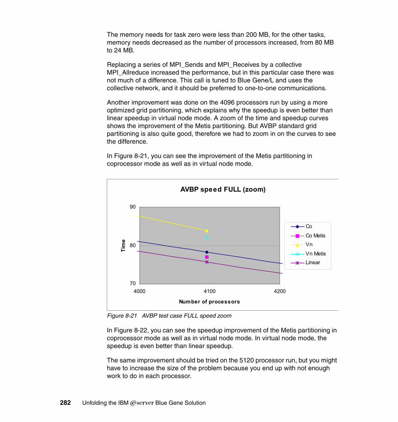
The memory needs for task zero were less than 200 MB, for the other tasks, memory needs decreased as the number of processors increased, from 80 MB to 24 MB.

Replacing a series of MPI_Sends and MPI_Receives by a collective MPI_Allreduce increased the performance, but in this particular case there was not much of a difference. This call is tuned to Blue Gene/L and uses the collective network, and it should be preferred to one-to-one communications.

Another improvement was done on the 4096 processors run by using a more optimized grid partitioning, which explains why the speedup is even better than linear speedup in virtual node mode. A zoom of the time and speedup curves shows the improvement of the Metis partitioning. But AVBP standard grid partitioning is also quite good, therefore we had to zoom in on the curves to see the difference.

In Figure 8-21, you can see the improvement of the Metis partitioning in coprocessor mode as well as in virtual node mode.

Figure 8-21 AVBP test case FULL speed zoom

In Figure 8-22, you can see the speedup improvement of the Metis partitioning in coprocessor mode as well as in virtual node mode. In virtual node mode, the speedup is even better than linear speedup.

The same improvement should be tried on the 5120 processor run, but you might have to increase the size of the problem because you end up with not enough work to do in each processor.

AVBP speed FULL (zoom)

70

80

90

4000 4100 4200


Tim

e

Co

Co MetisVn

Vn MetisLinear


Figure 8-22 AVBP test case FULL speedup zoom

An MPI trace of message exchanges shows that the application perfectly fits Blue Gene/L, with little room for improvement through tuning. The black areas in Figure 8-23 are computation, while the colored areas communication time. This is the trace for the 512 nodes.

Figure 8-23 MPI trace for message exchange

AVBP speedup FULL (zoom)

3800

3900

4000

4100

4200

4000 4100 4200


Spee

dup

Co

Co Metis

Vn

Vn Metis

Linear


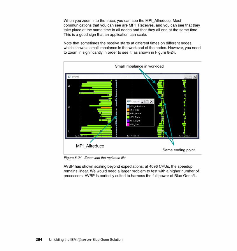
When you zoom into the trace, you can see the MPI_Allreduce. Most communications that you can see are MPI_Receives, and you can see that they take place at the same time in all nodes and that they all end at the same time. This is a good sign that an application can scale.

Note that sometimes the receive starts at different times on different nodes, which shows a small imbalance in the workload of the nodes. However, you need to zoom in significantly in order to see it, as shown in Figure 8-24.

Figure 8-24 Zoom into the mpitrace file

AVBP has shown scaling beyond expectations; at 4096 CPUs, the speedup remains linear. We would need a larger problem to test with a higher number of processors. AVBP is perfectly suited to harness the full power of Blue Gene/L.

MPI_Allreduce

Small imbalance in workload

Same ending point


8.5 LS-DYNALS-DYNA is finite element software for analyzing large deformation dynamic response (nonlinear dynamic analysis) of structures in three dimensions.

8.5.1 IntroductionLS-DYNA is used to solve multi-physics problems including solid mechanics, heat transfer, and fluid dynamics, either as separate phenomena or as coupled physics, for example, thermal stress or fluid structure interaction.

For details refer to LS-DYNA Keyword Reference Manual, and LS-DYNA Theory Manual created by the Livermore Software Technology Corporation, available online at:

http://www.lstc.com

The main LS-DYNA application domains include:

� Automotive crash-worthiness and occupant safety

� Airbags, seatbelts, occupants (dummies), car deformations

� Sheet metal formation

� Metal stamping, hydro forming, forging, multi-stage processes

� Military and defense applications

� Projectile (and armor) penetration problems, explosives, weapon design

� Aerospace industry applications

� Blade containment, bird strike, failure analyses

� Fluid dynamics

8.5.2 Parallel implementation of LS-DYNALS-DYNA implements an explicit integration scheme, in which a combined finite element approach typically performs the contact computation, internal forces computation, external forces computation, temporal integration, and configuration update.

In implementing LS-DYNA on a distributed computer, a client/server model is used in which the server task reads the discretized mesh of the physical domain, partitions the mesh, distributes it to all the client tasks running on other compute nodes, and monitors the progress of the computation.

The decomposition methods help to achieve load balance and to minimize the communication among the partitions. The finite element structure is decomposed


into n parts, in order to have a computation on n processors. The decomposition algorithm used in this investigation is Recursive Coordinate Bisection (RCB).

After initial data is distributed by the server task, the local element computations (including contact, internal force, external load, and nodal displacement calculations) are conducted in each client task as a sequential calculation. The client tasks exchange information with one another and the server process during each time step.

8.5.3 Running LS-DYNA on BG/LUsing the mpirun command, described in 4.4, “Scheduling (running) jobs” on page 77, you can submit LS-DYNA job on Blue Gene/L. The syntax of the job invocation is given in Example 8-3

Example 8-3 LS-DYNA Invocation Syntax

$ mpirun -np p ls-dyna_mpp_program i=input_file_name, p=pfile_name or $ mpirun -np p ls-dyna_mpp_program i=input_file_name

where p is the number of processors,

input_file_name is the LS-DYNA MPP data file (with nodes, elements, material cards...) and

pfile_name is the optional file which specifies the decomposition methodused to partition the finite element model into subdomains.

Impact of limited memory on compute nodesThe memory on each compute node in the Blue Gene/L is 512 M Bytes or 256 M Bytes when operating in a co-processor or virtual node modes respectively. As described in the previous section, server node reads the model before partitioning it into subdomains. For large models, the memory requirements to read the entire model can exceed the limited memory available for each task on a Blue Gene/L node.

LD-DYNA offers a facility to do the decomposition of the finite element structure separately on a workstation that has more memory. Also, it can be useful to make the decomposition of the finite element structure separately: the parallel computer is not tied up while the decomposition is taking place. After the decomposition is done, a file *.pre is created. The problem will not actually be run; instead, the code will terminate once the decomposition is achieved.

The server process in LS-DYNA running on Blue Gene/L reads this file and distributes the partition information to the client tasks. Since the server process does not have to do the decomposition, the memory requirement is reduced


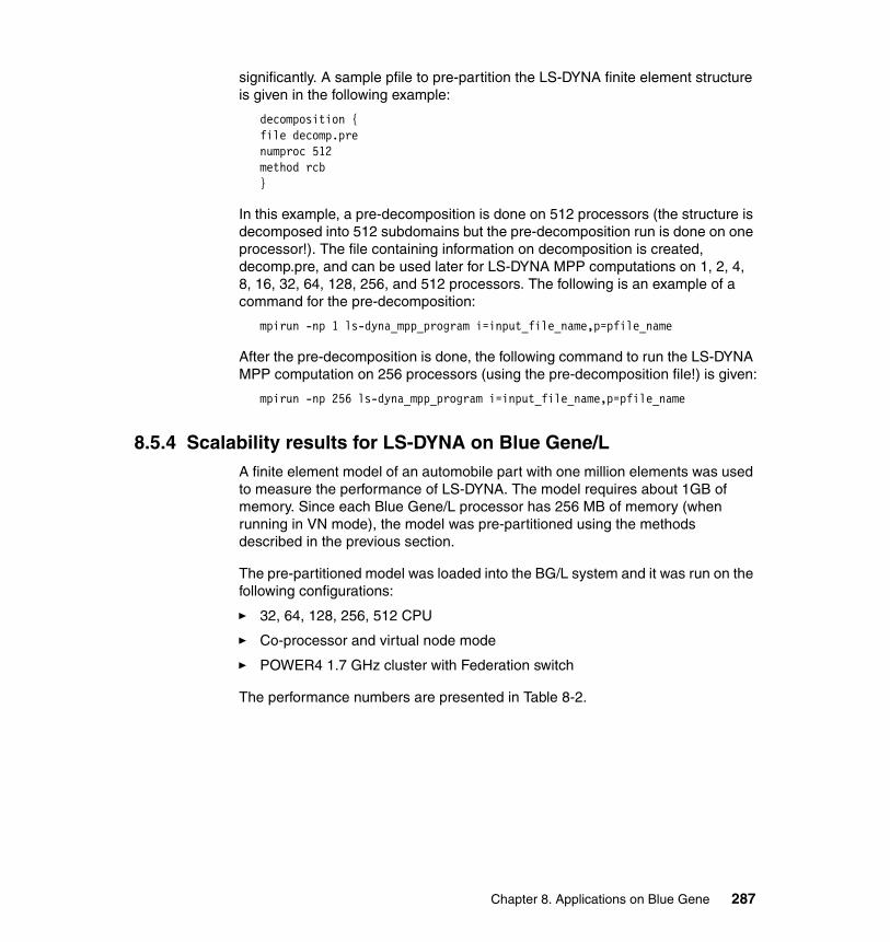
significantly. A sample pfile to pre-partition the LS-DYNA finite element structure is given in the following example:

decomposition { file decomp.pre numproc 512method rcb }

In this example, a pre-decomposition is done on 512 processors (the structure is decomposed into 512 subdomains but the pre-decomposition run is done on one processor!). The file containing information on decomposition is created, decomp.pre, and can be used later for LS-DYNA MPP computations on 1, 2, 4, 8, 16, 32, 64, 128, 256, and 512 processors. The following is an example of a command for the pre-decomposition:

mpirun -np 1 ls-dyna_mpp_program i=input_file_name,p=pfile_name

After the pre-decomposition is done, the following command to run the LS-DYNA MPP computation on 256 processors (using the pre-decomposition file!) is given:

mpirun -np 256 ls-dyna_mpp_program i=input_file_name,p=pfile_name

8.5.4 Scalability results for LS-DYNA on Blue Gene/LA finite element model of an automobile part with one million elements was used to measure the performance of LS-DYNA. The model requires about 1GB of memory. Since each Blue Gene/L processor has 256 MB of memory (when running in VN mode), the model was pre-partitioned using the methods described in the previous section.

The pre-partitioned model was loaded into the BG/L system and it was run on the following configurations:

� 32, 64, 128, 256, 512 CPU

� Co-processor and virtual node mode

� POWER4 1.7 GHz cluster with Federation switch

The performance numbers are presented in Table 8-2.


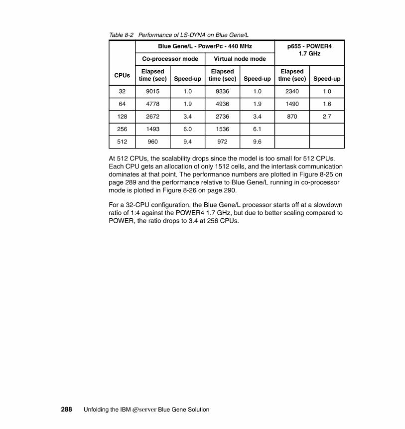
Table 8-2 Performance of LS-DYNA on Blue Gene/L

At 512 CPUs, the scalability drops since the model is too small for 512 CPUs. Each CPU gets an allocation of only 1512 cells, and the intertask communication dominates at that point. The performance numbers are plotted in Figure 8-25 on page 289 and the performance relative to Blue Gene/L running in co-processor mode is plotted in Figure 8-26 on page 290.

For a 32-CPU configuration, the Blue Gene/L processor starts off at a slowdown ratio of 1:4 against the POWER4 1.7 GHz, but due to better scaling compared to POWER, the ratio drops to 3.4 at 256 CPUs.

CPUs

Blue Gene/L - PowerPc - 440 MHz p655 - POWER41.7 GHz

Co-processor mode Virtual node mode

Elapsedtime (sec) Speed-up

Elapsed time (sec) Speed-up

Elapsed tIme (sec) Speed-up

32 9015 1.0 9336 1.0 2340 1.0

64 4778 1.9 4936 1.9 1490 1.6

128 2672 3.4 2736 3.4 870 2.7

256 1493 6.0 1536 6.1

512 960 9.4 972 9.6


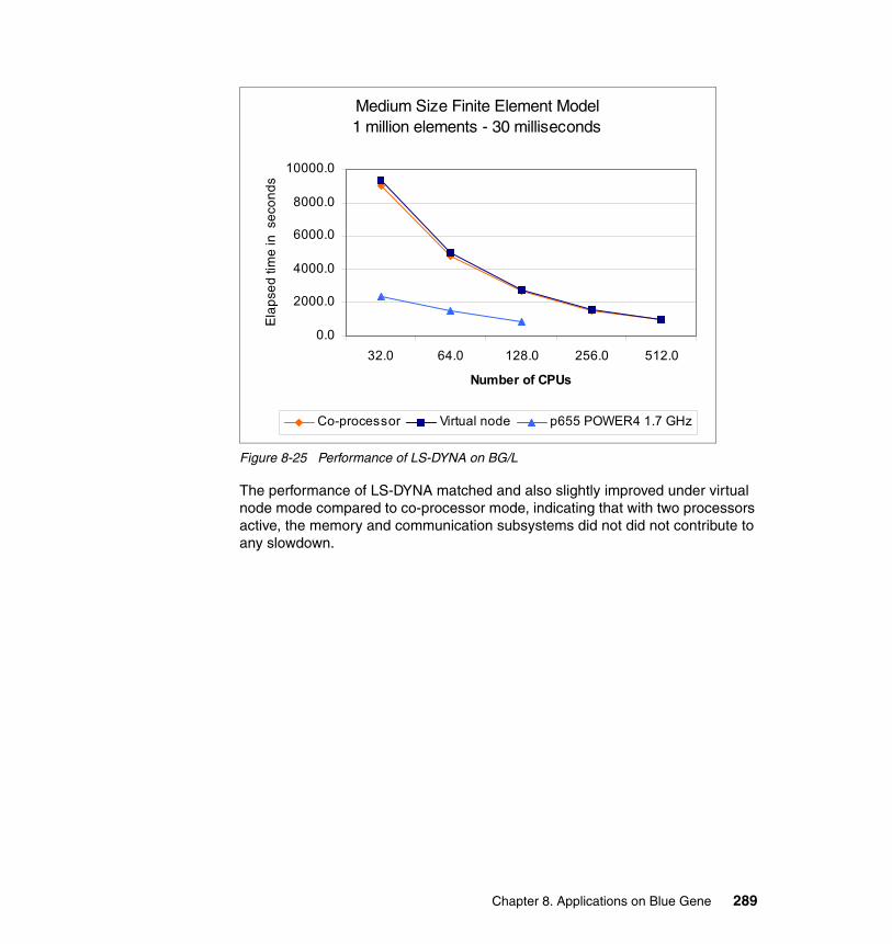
Figure 8-25 Performance of LS-DYNA on BG/L

The performance of LS-DYNA matched and also slightly improved under virtual node mode compared to co-processor mode, indicating that with two processors active, the memory and communication subsystems did not did not contribute to any slowdown.

Medium Size Finite Element Model1 million elements - 30 milliseconds

0.0

2000.0

4000.0

6000.0

8000.0

10000.0

32.0 64.0 128.0 256.0 512.0

Number of CPUs

Ela

pse

d ti

me

in s

eco

nd

s

Co-processor Virtual node p655 POWER4 1.7 GHz


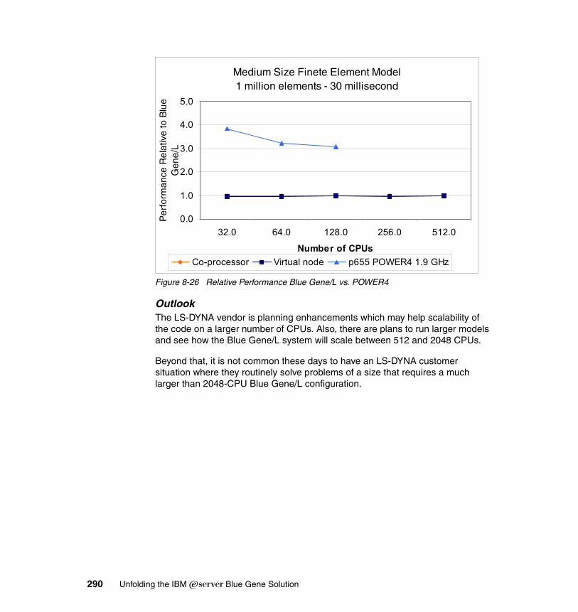
Figure 8-26 Relative Performance Blue Gene/L vs. POWER4

OutlookThe LS-DYNA vendor is planning enhancements which may help scalability of the code on a larger number of CPUs. Also, there are plans to run larger models and see how the Blue Gene/L system will scale between 512 and 2048 CPUs.

Beyond that, it is not common these days to have an LS-DYNA customer situation where they routinely solve problems of a size that requires a much larger than 2048-CPU Blue Gene/L configuration.

Medium Size Finete Element Model1 million elements - 30 millisecond

0.0

1.0

2.0

3.0

4.0

5.0

32.0 64.0 128.0 256.0 512.0

Number of CPUs

Per

form

ance

Rel

ativ

e to

Blu

e G

ene/

L

Co-processor Virtual node p655 POWER4 1.9 GHz


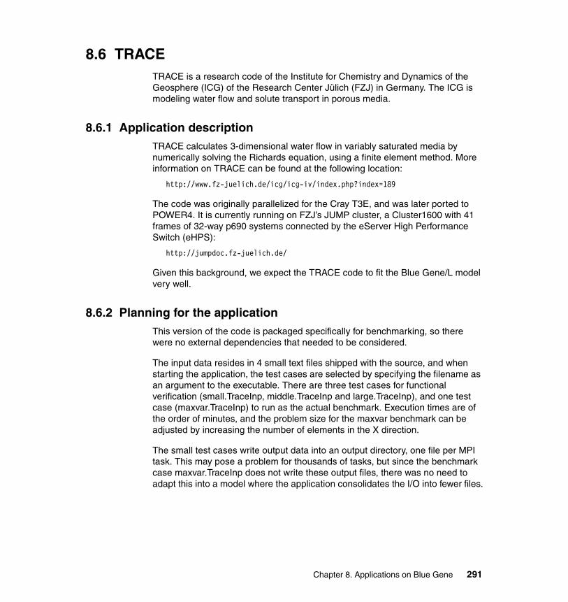
8.6 TRACETRACE is a research code of the Institute for Chemistry and Dynamics of the Geosphere (ICG) of the Research Center Jülich (FZJ) in Germany. The ICG is modeling water flow and solute transport in porous media.

8.6.1 Application descriptionTRACE calculates 3-dimensional water flow in variably saturated media by numerically solving the Richards equation, using a finite element method. More information on TRACE can be found at the following location:

http://www.fz-juelich.de/icg/icg-iv/index.php?index=189

The code was originally parallelized for the Cray T3E, and was later ported to POWER4. It is currently running on FZJ’s JUMP cluster, a Cluster1600 with 41 frames of 32-way p690 systems connected by the eServer High Performance Switch (eHPS):

http://jumpdoc.fz-juelich.de/

Given this background, we expect the TRACE code to fit the Blue Gene/L model very well.

8.6.2 Planning for the applicationThis version of the code is packaged specifically for benchmarking, so there were no external dependencies that needed to be considered.

The input data resides in 4 small text files shipped with the source, and when starting the application, the test cases are selected by specifying the filename as an argument to the executable. There are three test cases for functional verification (small.TraceInp, middle.TraceInp and large.TraceInp), and one test case (maxvar.TraceInp) to run as the actual benchmark. Execution times are of the order of minutes, and the problem size for the maxvar benchmark can be adjusted by increasing the number of elements in the X direction.

The small test cases write output data into an output directory, one file per MPI task. This may pose a problem for thousands of tasks, but since the benchmark case maxvar.TraceInp does not write these output files, there was no need to adapt this into a model where the application consolidates the I/O into fewer files.


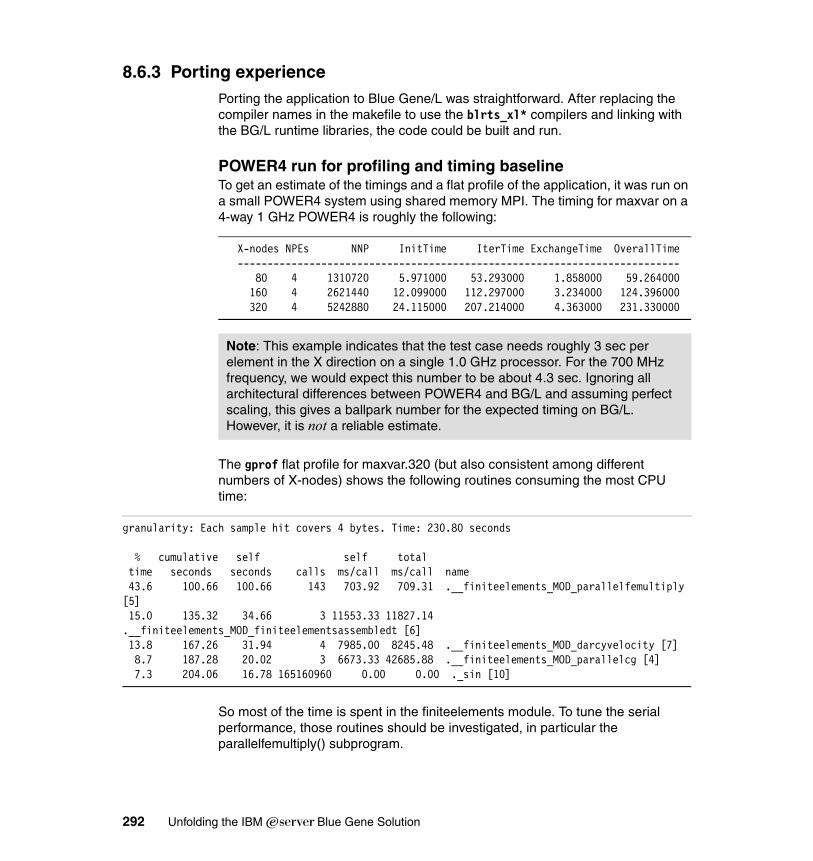
8.6.3 Porting experiencePorting the application to Blue Gene/L was straightforward. After replacing the compiler names in the makefile to use the blrts_xl* compilers and linking with the BG/L runtime libraries, the code could be built and run.

POWER4 run for profiling and timing baselineTo get an estimate of the timings and a flat profile of the application, it was run on a small POWER4 system using shared memory MPI. The timing for maxvar on a 4-way 1 GHz POWER4 is roughly the following:

X-nodes NPEs NNP InitTime IterTime ExchangeTime OverallTime--------------------------------------------------------------------------

80 4 1310720 5.971000 53.293000 1.858000 59.264000160 4 2621440 12.099000 112.297000 3.234000 124.396000320 4 5242880 24.115000 207.214000 4.363000 231.330000

The gprof flat profile for maxvar.320 (but also consistent among different numbers of X-nodes) shows the following routines consuming the most CPU time:

granularity: Each sample hit covers 4 bytes. Time: 230.80 seconds

% cumulative self self total time seconds seconds calls ms/call ms/call name 43.6 100.66 100.66 143 703.92 709.31 .__finiteelements_MOD_parallelfemultiply [5] 15.0 135.32 34.66 3 11553.33 11827.14 .__finiteelements_MOD_finiteelementsassembledt [6] 13.8 167.26 31.94 4 7985.00 8245.48 .__finiteelements_MOD_darcyvelocity [7] 8.7 187.28 20.02 3 6673.33 42685.88 .__finiteelements_MOD_parallelcg [4] 7.3 204.06 16.78 165160960 0.00 0.00 ._sin [10]

So most of the time is spent in the finiteelements module. To tune the serial performance, those routines should be investigated, in particular the parallelfemultiply() subprogram.

Note: This example indicates that the test case needs roughly 3 sec per element in the X direction on a single 1.0 GHz processor. For the 700 MHz frequency, we would expect this number to be about 4.3 sec. Ignoring all architectural differences between POWER4 and BG/L and assuming perfect scaling, this gives a ballpark number for the expected timing on BG/L. However, it is not a reliable estimate.


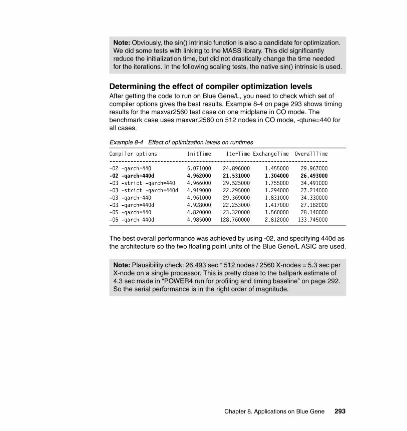
Determining the effect of compiler optimization levelsAfter getting the code to run on Blue Gene/L, you need to check which set of compiler options gives the best results. Example 8-4 on page 293 shows timing results for the maxvar2560 test case on one midplane in CO mode. The benchmark case uses maxvar.2560 on 512 nodes in CO mode, -qtune=440 for all cases.

Example 8-4 Effect of optimization levels on runtimes

Compiler options InitTime IterTime ExchangeTime OverallTime--------------------------------------------------------------------------O2 -qarch=440 5.071000 24.896000 1.455000 29.967000-O2 -qarch=440d 4.962000 21.531000 1.304000 26.493000-O3 -strict -qarch=440 4.966000 29.525000 1.755000 34.491000-O3 -strict -qarch=440d 4.919000 22.295000 1.294000 27.214000-O3 -qarch=440 4.961000 29.369000 1.831000 34.330000-O3 -qarch=440d 4.928000 22.253000 1.417000 27.182000-O5 -qarch=440 4.820000 23.320000 1.560000 28.140000-O5 -qarch=440d 4.985000 128.760000 2.812000 133.745000

The best overall performance was achieved by using -02, and specifying 440d as the architecture so the two floating point units of the Blue Gene/L ASIC are used.

Note: Obviously, the sin() intrinsic function is also a candidate for optimization. We did some tests with linking to the MASS library. This did significantly reduce the initialization time, but did not drastically change the time needed for the iterations. In the following scaling tests, the native sin() intrinsic is used.

Note: Plausibility check: 26.493 sec * 512 nodes / 2560 X-nodes = 5.3 sec per X-node on a single processor. This is pretty close to the ballpark estimate of 4.3 sec made in “POWER4 run for profiling and timing baseline” on page 292. So the serial performance is in the right order of magnitude.


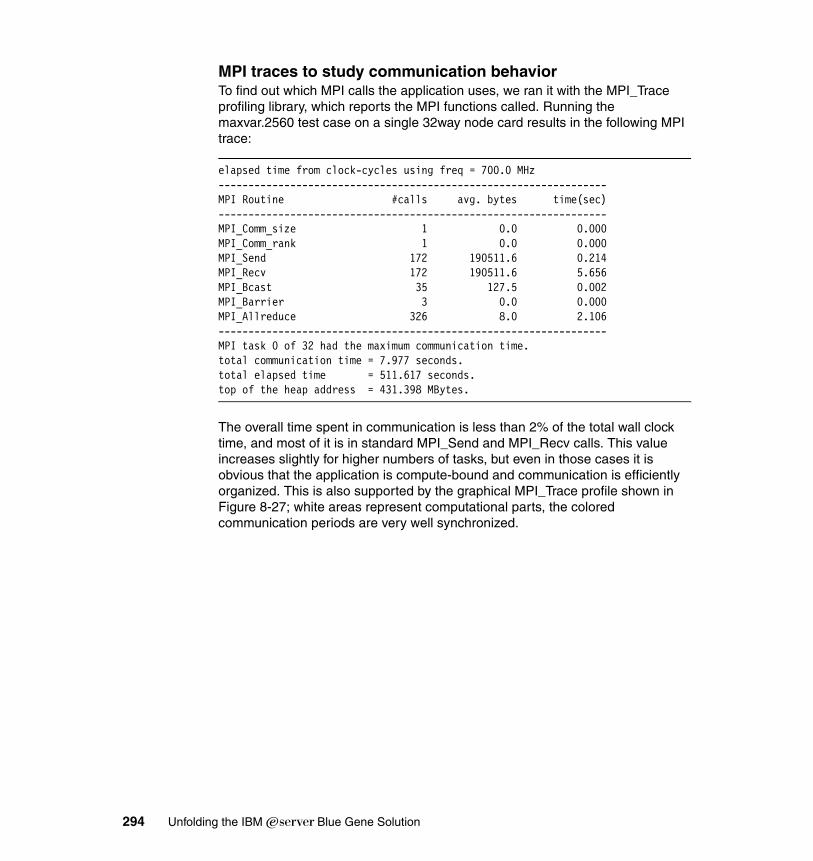
MPI traces to study communication behaviorTo find out which MPI calls the application uses, we ran it with the MPI_Trace profiling library, which reports the MPI functions called. Running the maxvar.2560 test case on a single 32way node card results in the following MPI trace:

elapsed time from clock-cycles using freq = 700.0 MHz-----------------------------------------------------------------MPI Routine #calls avg. bytes time(sec)-----------------------------------------------------------------MPI_Comm_size 1 0.0 0.000MPI_Comm_rank 1 0.0 0.000MPI_Send 172 190511.6 0.214MPI_Recv 172 190511.6 5.656MPI_Bcast 35 127.5 0.002MPI_Barrier 3 0.0 0.000MPI_Allreduce 326 8.0 2.106-----------------------------------------------------------------MPI task 0 of 32 had the maximum communication time.total communication time = 7.977 seconds.total elapsed time = 511.617 seconds.top of the heap address = 431.398 MBytes.

The overall time spent in communication is less than 2% of the total wall clock time, and most of it is in standard MPI_Send and MPI_Recv calls. This value increases slightly for higher numbers of tasks, but even in those cases it is obvious that the application is compute-bound and communication is efficiently organized. This is also supported by the graphical MPI_Trace profile shown in Figure 8-27; white areas represent computational parts, the colored communication periods are very well synchronized.


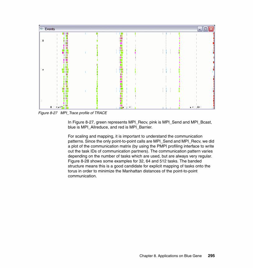
Figure 8-27 MPI_Trace profile of TRACE

In Figure 8-27, green represents MPI_Recv, pink is MPI_Send and MPI_Bcast, blue is MPI_Allreduce, and red is MPI_Barrier.

For scaling and mapping, it is important to understand the communication patterns. Since the only point-to-point calls are MPI_Send and MPI_Recv, we did a plot of the communication matrix (by using the PMPI profiling interface to write out the task IDs of communication partners). The communication pattern varies depending on the number of tasks which are used, but are always very regular. Figure 8-28 shows some examples for 32, 64 and 512 tasks. The banded structure means this is a good candidate for explicit mapping of tasks onto the torus in order to minimize the Manhattan distances of the point-to-point communication.


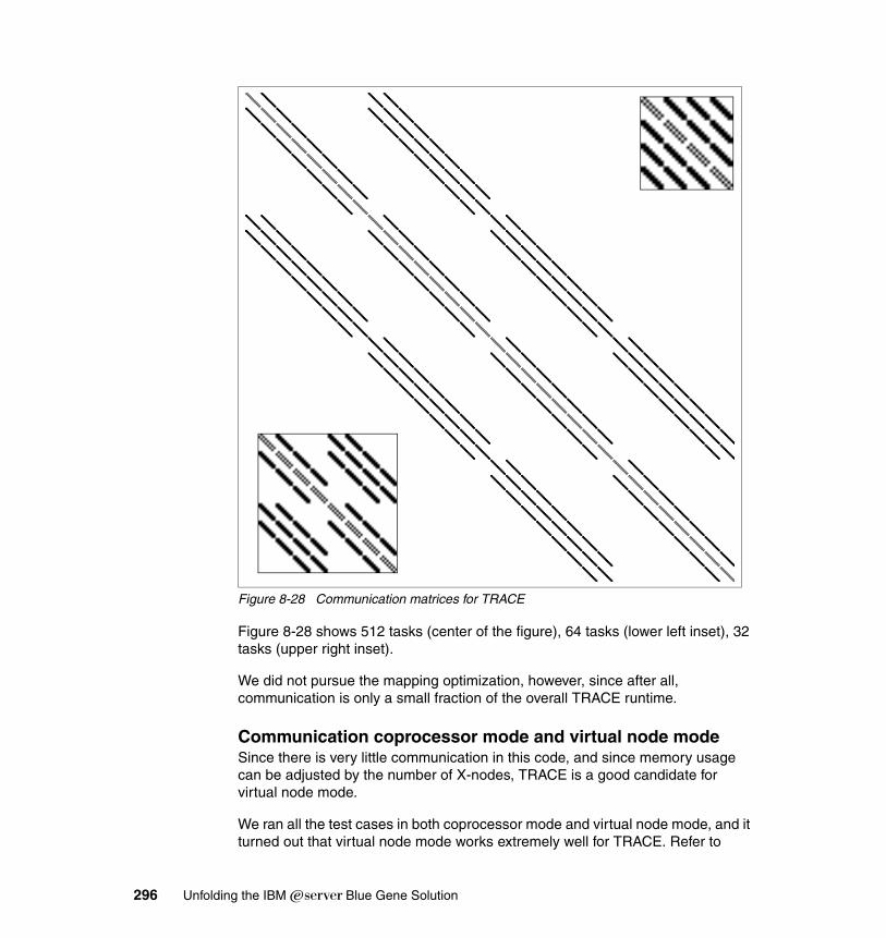
Figure 8-28 Communication matrices for TRACE

Figure 8-28 shows 512 tasks (center of the figure), 64 tasks (lower left inset), 32 tasks (upper right inset).

We did not pursue the mapping optimization, however, since after all, communication is only a small fraction of the overall TRACE runtime.

Communication coprocessor mode and virtual node modeSince there is very little communication in this code, and since memory usage can be adjusted by the number of X-nodes, TRACE is a good candidate for virtual node mode.

We ran all the test cases in both coprocessor mode and virtual node mode, and it turned out that virtual node mode works extremely well for TRACE. Refer to


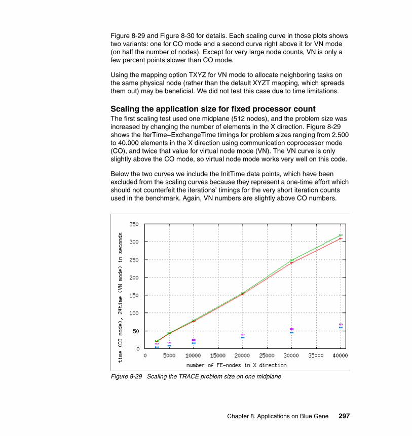
Figure 8-29 and Figure 8-30 for details. Each scaling curve in those plots shows two variants: one for CO mode and a second curve right above it for VN mode (on half the number of nodes). Except for very large node counts, VN is only a few percent points slower than CO mode.

Using the mapping option TXYZ for VN mode to allocate neighboring tasks on the same physical node (rather than the default XYZT mapping, which spreads them out) may be beneficial. We did not test this case due to time limitations.

Scaling the application size for fixed processor countThe first scaling test used one midplane (512 nodes), and the problem size was increased by changing the number of elements in the X direction. Figure 8-29 shows the IterTime+ExchangeTime timings for problem sizes ranging from 2.500 to 40.000 elements in the X direction using communication coprocessor mode (CO), and twice that value for virtual node mode (VN). The VN curve is only slightly above the CO mode, so virtual node mode works very well on this code.

Below the two curves we include the InitTime data points, which have been excluded from the scaling curves because they represent a one-time effort which should not counterfeit the iterations’ timings for the very short iteration counts used in the benchmark. Again, VN numbers are slightly above CO numbers.

Figure 8-29 Scaling the TRACE problem size on one midplane


The diagram in Figure 8-29 is running in co-processor node mode and virtual node mode. Solid lines show IterTime+ExchengeTime, isolated datapoints show InitTime.

The benchmark case with 50.000 elements in the X direction could not be run on a single midplane due to memory constraints. This is in agreement with the estimated memory consumption of this code:

memory usage/task (MB) = #x-nodes / #tasks * 5.84 + 11.5 MB#x-nodes = #tasks * (memory - 11.5 MB) / 5.84

This estimate had been used for previous benchmarks; for 512 nodes with about 500 MB of usable memory, about 43000 X-nodes can be simulated.

Scaling to large processor countsThe main scaling test for Blue Gene/L is to vary the number of nodes used to solve a problem of a fixed size. In Figure 8-30, we show this data for problem sizes of 10000, 20000, 30000, and 40000 elements in the X direction. Plotting the elapsed time multiplied with the number of nodes should ideally result in a constant curve for each problem size. The measured performance shows very good scaling indeed.

Figure 8-30 Scaling the number of tasks for TRACE


Total CPU time for problem sizes (X-nodes) of 10000, 20000, 30000, 40000, and 50.000 (one datapoint only), CP mode, and VN mode with XYZT mapping are shown.

We used both CO mode and VN mode. Again the VN curves are the ones slightly above the CO curves. For the runs using four Blue Gene/L racks, VN mode appears to become more inefficient and departs significantly from CO mode curves.

In summary, TRACE fits well on the Blue Gene/L system and can be easily scaled to thousands of processors. However, at high processor counts, it becomes obvious that the data arrays in the code which are replicated across all tasks become more and more of a limiting factor. For this reason we were unable to further increase the problem size: the 50.000 X-elements case could be run on one rack, but consumed too much memory per node on 2 racks.

To further scale the TRACE code, the replicated arrays would need to be investigated. If some of them can be distributed instead of replicating them across all nodes, it should be possible to further scale both the problem sizes and number of tasks used for the solution.

8.7 CPMDThe CPMD code is based on the original computer code written by Car and Parrinello5. It was developed first at the IBM Research Zurich laboratory, in collaboration with many groups worldwide. It is a production code with many unique features written in FORTRAN 77, and has grown from its original size of approximately 10,000 lines to currently close to 200,000 lines of code. Since January 2002, the program has been freely available for non-commercial use6 (see also http://www.cpmd.org). Several thousand registered users in more than 50 countries have compiled and run the code on platforms as diverse as notebooks and computers at the top of the TOP500 list (www.top500.org).

8.7.1 CPMD descriptionThe basics of the implementation of the Kohn-Sham method using a plane-wave basis set and pseudopotentials are described in several review articles7, and the CPMD code follows them closely. All standard gradient-corrected density

5 See: R. Car, M. Parrinello, Phys. Rev. Lett., 1985, 55, 2471-2474 6 See: CPMD V3.9, Copyright IBM Corp. 1990-2003, Copyright MPI fur Festkorperforschung, Stuttgart, 1997-20017 See: D. Marx, J. Hutter, Ab-initio molecular dynamics: Theory and implementation, in: Modern Methods and Algorithms of Quantum Chemistry, J. Grotendorst (Ed.), NIC Series, Vol. 1, FZ Julich, Germany, 2000; see also: http://www.fz-juelich.de/nic-series/Volume and references therein.


functionals are supported, and preliminary support for functionals that depend on the kinetic energy density is available. Pseudopotentials used in CPMD are either of the norm-conserving or the ultra-soft type8. Norm-conserving pseudopotentials have been the default method in CPMD, and only some of the rich functionality has been implemented for ultra-soft pseudopotentials.

The emphasis of CPMD on MD simulations of complex structures and liquids led to the optimization of the code for large supercells and a single k-point (the k = 0 point) approximation. Many features have therefore only been implemented for this special case. CPMD has a rich set of features, many of them unique. For a complete overview the reader is referred to the manual (see CPMD V3.9, Copyright IBM Corp. 1990-2003, Copyright MPI fur Festkorperforschung Stuttgart, 1997-2001, see also http://www.cpmd.org). The basic electronic structure method implemented uses fixed occupation numbers, either within a spin-restricted or an unrestricted scheme. For systems with variable occupation number (small gap systems and metals), the free energy functional9 can be used together with iterative diagonalization methods.

On top of the basic scheme, a fine-grained, shared-memory parallelization was implemented. The two parallelization methods are independent and can be mixed. This makes it possible to achieve good performance on distributed computers with shared memory nodes and several thousands of CPUs, as well as to extend the size of the systems that can be studied completely ab initio to several thousand atoms10.

Another parallelization strategy is targeted at the loop over electronic states needed for the calculation of the charge density and the application of the local potential. For small- and medium-sized systems, the three-dimensional Fourier transform (3dFFT) within these loops dominates the computational costs. Parallelization of the 3dFFT is either limited by load balancing (if a coarse-grained approach is followed) or by latency (in the case of fine-grain parallelization). In CPMD, the parallelization of the outer loop over electronic states can be combined with the parallelization of the 3dFFT. This approach (called Taskgroups) is especially suited for massively parallel computers with balanced architectures, as BG/L, if used in combination with optimal mapping.

Some methods implemented in CPMD allow a further level of parallelization. Methods such as path-integral molecular dynamics or linear response theory are embarrassingly parallel on the level of the energy calculation. Typically, two to 32 copies of the energy and force calculation can be run in parallel. For these methods, an efficient use of computers with tens of thousands of CPUs can be envisaged.

8 See: D. Vanderbilt, Phys. Rev. B, 1990, 41, 7892-7895.9 ( see: A. Alavi, J. Kohanoff, M. Parrinello, D. Frenkel, Phys. Rev. Lett., 1994, 73, 2599-2602)10 see : J. Hutter and A.Curioni, Parallel Computing, 2004


The coarse-grained, distributed-memory parallelization is driven by the distribution of wave-function coefficients for all states to all CPUs. Real-space grids are also distributed, whereas all matrices that do not include a plane-wave index are replicated (especially overlap matrices). All other arrays are only distributed if this does not cause additional communications. With this scheme, all loops communicate over plane waves, especially the ones having an N2M scaling, where M is the number of plane waves and N the number of atoms, states or pseudopotential projectors. This scheme explicitly requires a parallel 3dFFT.

Further requirements to optimize the Fourier transforms are used to find the optimal data distribution. The 3dFFT can be seen as performing the following steps:

1. Scatter of data C(x, y, z) - c(G).

2. Transformations along direction x.

3. Transformations along direction y.

4. Transformations along direction z.

For a general data distribution in both spaces, each of the steps would include communication between all processors. The data distribution in CPMD minimizes the number of communication steps while maintaining optimum load balancing in both spaces. To achieve this goal, the following requirements have to be fulfilled:

� Each processor hosts the same number of plane waves.

� All plane waves with common y and z components are located on the same processor.

� The number of different (y, z) pairs of plane-wave components is the same on each processor.

� A processor hosts full planes of real-space grid points.

The number of real-space planes is the same on each processor. This scheme requires only a single data communication step after the first (or before the last) 1D transform. In addition, you can make use of the sparsity of the wave-function representation still present after the first transform and only communicate nonzero elements. The various load-balancing requirements are interrelated, and a heuristic algorithm to achieve near-optimum results is used.

The restriction to full-plane distributions in real space, however, introduces severe problems in the case of a large number of processors. The number of planes available is typically about 50 for small systems and 200 to 2000 for large systems. This restricts the maximum number of processors that can be used efficiently.


The efficiency of the basic scheme is limited, owing to the following problems: Global summation of overlap matrices and broadcast of matrices scale as Npe logNpe and will become predominant for large numbers of processors (Npe). The calculation of the rotation matrix in the SHAKE/RATTLE11 algorithm is not parallel and limits the maximum speedup that can be achieved. Replicated overlap matrices might become a memory bottleneck for large systems on many processors with small memory.

The maximum number of grid points in a direction limits the maximum number of processors that can be used efficiently for the 3dFFT. The time required for the all-to-all communications scales as Npe Latency, downgrading the performance scaling in the case of communication adapters with relatively high latency.

8.7.2 Application characterizationSince this is an MPI application, we need to ask the following questions:

Q: What level of scalability is typically seen on distributed memory systems (number of processors)?

A: Results on diverse physical systems having sizes ranging from 100 to 1000 atoms exhibit good scalability to thousands of processors and molecular dynamics throughputs ranging from 2 to 200 ps/week. Parallel efficiency of ~90% up to 1000 processors and ~60% up to 4000 processors has been measured.

Q: How much interprocessor communication, and what type of communication is expected (that is, shmem, mpi_send, reductions, global sum, global array, and so forth)?

A: This depends on the system size and on the type of parallelization used (meaning use of taskgroups or not), mainly all-to-all and global reductions.

Q: Is there a typical ratio of computation-to-communication that characterizes this application?

A: This depends on the system size and on the type of parallelization used. The ratio for small systems is dominated by 3D-FFT computation; for large systems (linear algebra) communication becomes dominant. In any case, both computation and communication are intensive.

11 (See: J. Hutter, M. E. Tuckerman, and M. Parrinello, J. Chem. Phys. 1995, 102, 859-871)

Note: This problem has been solved on BG/L by using a distributed matrix algorithm for the rotation matrix.


8.7.3 Enablement experience and test resultsThe tests performed show the performance and scaling data on Blue Gene/L in comparison with POWER5 on small systems.

Following are the main steps required to enable CPMD to Blue Gene/L:

1. Cleaning of memory allocation to preserve memory alignment.

2. Interface to FFTW-spiral, to use double hummer FFT.

3. Use PowerPC intrinsic for the zeroing of vectors.

4. Use double hummer routines for DGEMM and DCOPY.

5. Implement taskgroup parallelization with optimal mapping.

6. Distribution of overlap matrices and parallelization of orthogonalization.

The optimized code (binary) is distributed to selected customers by IBM Zurich; full support and distribution of the source code is planned for the general version for 3Q05.

8.7.4 Benchmark DataThe benchmarks used here to determine scalability were carried out on different systems. The first is a clustered SMP server, which is an ideal testbed for the dual-level parallelization scheme. This system consists of 40 IBM pSeries 690 32-way servers (based on the POWER4 1.3 GHz processor), logically partitioned in 160 8-way SMP nodes, connected via dual-channel colony switches (Phase I system at HPCx- Daresbury). This results in an aggregate compute power of 5.2 TFlop/s.

The second supercomputer is the novel IBM Blue Gene/L solution, consisting of 1024 dual-processor nodes based on the PowerPC 440 embedded processors with 700 MHz clock speed, resulting in an aggregate compute power of 5.6 TFlops.

The first system investigated is solid SiC with a supercell containing 216 atoms (~400 Kohn-Sham states), norm-conserving pseudopotentials and Becke-LYP functional; this system, which is relatively small, has been chosen to stress the scaling behavior. Note that the mixed MPI/SMP scheme has been used to scale out on the p690 system, whereas the taskgroup scheme with optimal mapping has been used on BG/L.

In Figure 8-31 we illustrate Blue Gene/L scalability, and we compare the other systems (only as a reference). It is important to realize that the full benefit of Blue Gene/L becomes apparent when we start looking at 512 processors and beyond.


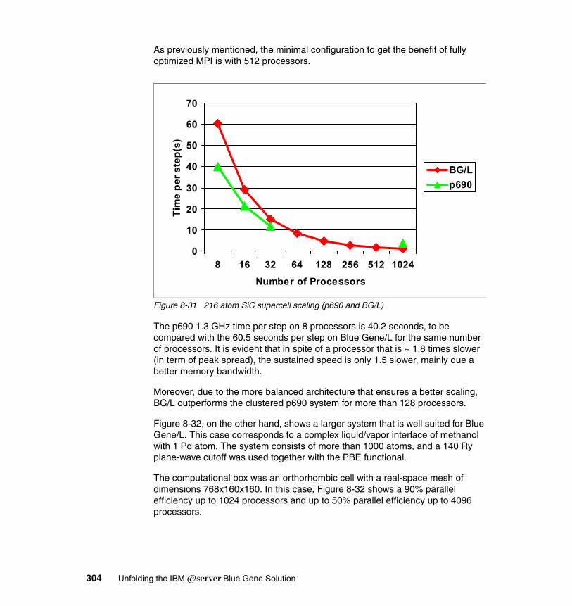
As previously mentioned, the minimal configuration to get the benefit of fully optimized MPI is with 512 processors.

Figure 8-31 216 atom SiC supercell scaling (p690 and BG/L)

The p690 1.3 GHz time per step on 8 processors is 40.2 seconds, to be compared with the 60.5 seconds per step on Blue Gene/L for the same number of processors. It is evident that in spite of a processor that is ~ 1.8 times slower (in term of peak spread), the sustained speed is only 1.5 slower, mainly due a better memory bandwidth.

Moreover, due to the more balanced architecture that ensures a better scaling, BG/L outperforms the clustered p690 system for more than 128 processors.

Figure 8-32, on the other hand, shows a larger system that is well suited for Blue Gene/L. This case corresponds to a complex liquid/vapor interface of methanol with 1 Pd atom. The system consists of more than 1000 atoms, and a 140 Ry plane-wave cutoff was used together with the PBE functional.

The computational box was an orthorhombic cell with a real-space mesh of dimensions 768x160x160. In this case, Figure 8-32 shows a 90% parallel efficiency up to 1024 processors and up to 50% parallel efficiency up to 4096 processors.

0

10

20

30

40

50

60

70

8 16 32 64 128 256 512 1024Number of Processors

Tim

e pe

r ste

p(s)

BG/Lp690


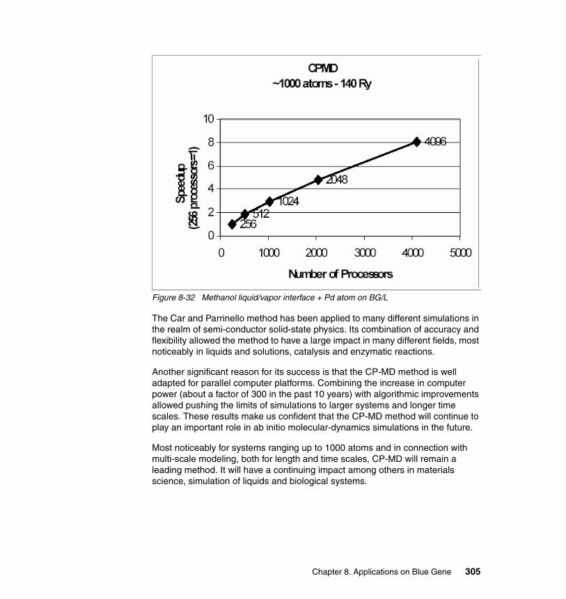
Figure 8-32 Methanol liquid/vapor interface + Pd atom on BG/L

The Car and Parrinello method has been applied to many different simulations in the realm of semi-conductor solid-state physics. Its combination of accuracy and flexibility allowed the method to have a large impact in many different fields, most noticeably in liquids and solutions, catalysis and enzymatic reactions.

Another significant reason for its success is that the CP-MD method is well adapted for parallel computer platforms. Combining the increase in computer power (about a factor of 300 in the past 10 years) with algorithmic improvements allowed pushing the limits of simulations to larger systems and longer time scales. These results make us confident that the CP-MD method will continue to play an important role in ab initio molecular-dynamics simulations in the future.

Most noticeably for systems ranging up to 1000 atoms and in connection with multi-scale modeling, both for length and time scales, CP-MD will remain a leading method. It will have a continuing impact among others in materials science, simulation of liquids and biological systems.


8.8 WRFWRF, or Weather and Research Forecast Model, is a weather code that is increasingly being used in climate modeling and weather forecasting. The code is the successor model to the popular weather code MM5 and comes from the NCAR - MMM division. The WRF Model is a next-generation mesocale numerical weather prediction system designed to serve both operational forecasting and atmospheric research needs.

The WRF development is a collaborative partnership, principally among the National Center for Atmospheric Research (NCAR), the National Oceanic and Atmospheric Administration (NOAA), the National Centers for Environmental Prediction (NCEP) and the Forecast Systems Laboratory (FSL), the Air Force Weather Agency (AFWA), the Naval Research Laboratory, Oklahoma University, and the Federal Aviation Administration (FAA).

8.8.1 Application descriptionThe latest version of the model is Version 2.0, and the most recent release of WRF V2.0.3.1 (December 2004) was used for performing the benchmark runs. WRF allows researchers the ability to conduct simulations reflecting either real data or idealized configurations. It features multiple dynamical cores, a 3-dimensional variational (3DVAR) data assimilation system, and a software architecture allowing for computational parallelism and system extensibility. WRF is suitable for a broad spectrum of applications across scales ranging from meters to thousands of kilometers.

Performance is model speed, ignoring I/O and initialization cost, directly measured as the average cost per time step over a representative period of model integration, and is presented as normalized floating-point rate and as simulation speed. The benchmarks are intended to provide a means for comparing the performance of different architectures and for comparing WRF computational performance and scaling with other models.

A representative period of model integration should be the smallest period that:

1. Includes all different types of time-step in the proportions they will occur for any length simulation

2. Provides a number of sequences of the complete set of time steps to reasonably represent performance variability stemming from varying states of the atmosphere being simulated and operational variability of the computer system itself

3. Steps far enough into a simulation to be considered spun-up

Floating-point rate provides a measure of efficiency relative to the theoretical peak capability of a computing system. It is the average number of floating-point


operations per time step divided by the average number of seconds per time step. Average floating-point operations per time step is determined by executing the test case over the integration period, counting the number of operations using the vendor’s hardware, and then dividing by the number of time steps in the integration period. The minimum over all systems measured is used for determining floating-point rate. Using a minimum avoids overstating performance and efficiency of the WRF code. The average time per time step is the sum of the times for each time step in the integration period divided by the number of time steps.

Scaling is the ratio of increase in simulation speed (or floating-point rate) to the increase in the number of parallel processes. A parallel process is the independent variable of this experiment. It is the unit of parallelism that is scaled up or down when running WRF on a parallel system.

WRF is currently in operational use at NCEP. For detailed information on this application, see:

http://www.wrf-model.org/index.php

8.8.2 CharacteristicsThe WRF model (and WRF 3DVAR) is written in FORTRAN (what many refer to as FORTRAN 90). A software layer, RSL, sits between WRF and the MPI interface and is written in C. There are also ancillary programs that are written in C to perform file parsing and file construction, both of which are required for default building of the WRF modeling code.

Additionally, the WRF build mechanism uses several scripting languages including perl (to handle various tasks such as the code browser designed by Brian Fiedler), Cshell, and Bourne shell. The traditional UNIX text/file processing utilities are used: make, M4, sed, and awk. There are several modes of build of WRF: MPI, OpenMP, and both MPI and OpenMP.

8.8.3 Planning for the applicationThe purpose of the benchmark effort was to port the WRF application to Blue Gene/L and perform test runs to show computational performance and scalability of the WRF model on the Blue Gene/L system. The code could be run with MPI and OpenMP. However, OpenMP is not supported on Blue Gene/L, and hence the MPI build of WRF was used on Blue Gene.

The code is a mix of FORTRAN and C languages, which in turn results in a requirement for FORTRAN and C compilers for building the code. The code uses


the NETCDF library, which has to be downloaded from the following link and built before attempting to build WRF:

http://my.unidata.ucar.edu/content/software/netcdf/index.html

8.8.4 Porting experience (depending on licensing)The code has been ported to AIX systems, but it has not been ported to Power on Linux, which is recommended before attempting on Blue Gene/L. The porting to Blue Gene is quite straightforward. You need to ensure that cross-compilation is enabled in configuration files, since configure is used for the builds of both Netcdf and WRF. You must also point to the right compiler and compiler options.

Building the NETCDF libraryNetCDF, or network Common Data Form, is an interface for array-oriented data access and a library that provides an implementation of the interface. The netCDF library also defines a machine-independent format for representing scientific data. Together the interface, library, and format support the creation, access, and sharing of scientific data.

A configure script is used for the build process, which will create system-dependent environment variables to be used for compilation like the compilers. Since we are cross-compiling, the cross-compile option should be set to yes in configure.

When configure is run, it creates a file, macros.make, which can be modified, if needed after configuring. It is recommended to use the same compilers for compiling netcdf as are used for building WRF. Example 8-5 shows a script that could be used for setting the environment variables when configuring your environment for compiling the code.

Example 8-5 A script to set environment variables for NETCDF build

#! /bin/kshexport CC='blrts_xlc'export CPPFLAGS='-D_POSIX_SOURCE -DNDEBUG -D_ALL_SOURCE'export FC=blrts_xlfexport F90=blrts_xlf90export CXX=blrts_xlCexport CFLAGS="-qarch=440"export FFLAGS="-O2 -qarch=440"export F90FLAGS="$FFLAGS -qsuffix=f=f90"./configure --prefix=/bgl/sheeba/lib/NETCDF

Variable description for Example 8-5:

CC C compiler


FC FORTRAN compiler F90 FORTRAN 90 compiler CXX C++ compilerCFLAGS C compiler flags CPPFLAGS C preprocessor options FFLAGS FORTRAN compiler flagsF90 fLAGS FORTRAN 90 compiler flags CXXFLAGS C++ compiler flags

Check the macros.make file to verify that all settings are for Blue Gene, and modify if needed. Normally while running configure, you would get a error message if it was not successful. Thereafter, issuing the commands make and make install will build and install the netcdf library in the directory that was passed by prefix.

Building WRFA configure.defaults file in the arch directory specifies the environment variables to be set for building WRF. This file was edited to introduce the new architecture, BG for Blue Gene system, and the environments corresponding to RSL and RSL_LITE were modified. The author used the AIX build options for POWER4, and this was modified to point to the right compilers and options for Blue Gene. Some of the points to keep in mind during build include:

� WRF provides a provides a provision for cross-compilation, and this option could be known from reading the configure script. (Remember, we are cross-compiling, and uname does not work and is not usable here.) Following are the environment variables that are to be set prior to building WRF:

export WRF_OS=BGexport WRF_MCH = 440export NETCDF=/bgl/sheeba/lib/NETCDF_xlc

� The -traditional flag is to be added to cpp flags if the preprocessor used is /lib/cpp, which comes with the GNU compiler. If you are using the preprocessor cpp that comes with the xlf compiler, there is no need to use this flag.

� Since there are a number of math function calls, for performance improvement, the code was linked with the mass libraries, libmass and libmassv.

� To get over the multiple definition error when linking with libmass, libmassv, add the flag for linking: -Wl,--allow-multiple-definition.

To profile the mpi trace library, we used libmpitrace_c.a from Bob Walkup (IBM Research). libmpitrace_f does not produce mpi_profiles because WRF is a mix of FORTRAN and C and some of the C codes make MPI calls. So it has to be linked with libmpitrace_c.a to generate the MPI trace files.


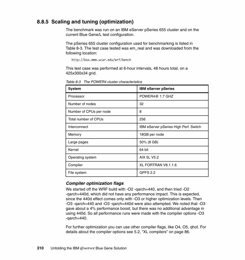
8.8.5 Scaling and tuning (optimization)The benchmark was run on an IBM eServer pSeries 655 cluster and on the current Blue Gene/L test configuration.

The pSeries 655 cluster configuration used for benchmarking is listed in Table 8-3. The test case tested was em_real and was downloaded from the following location:

http://box.mmm.ucar.edu/wrf/bench

This test case was performed at 6-hour intervals, 48 hours total, on a 425x300x34 grid.

Table 8-3 The POWER4 cluster characteristics

Compiler optimization flagsWe started off the WRF build with -O2 -qarch=440, and then tried -O2 -qarch=440d, which did not have any performance impact. This is expected, since the 440d effect comes only with -O3 or higher optimization levels. Then -O3 -qarch=440 and -O3 -qarch=440d were also attempted. We noted that -O3 gave about a 4% performance boost, but there was no additional advantage in using 440d. So all performance runs were made with the compiler options -O3 -qarch=440.

For further optimization you can use other compiler flags, like O4, O5, qhot. For details about the compiler options see 5.2, “XL compilers” on page 86.

System IBM eServer pSeries

Processor POWER4@ 1.7 GHZ

Number of nodes 32

Number of CPUs per node 8

Total number of CPUs 256

Interconnect IBM eServer pSeries High Perf. Switch

Memory 18GB per node

Large pages 50% (8 GB)

Kernel 64 bit

Operating system AIX 5L V5.2

Compiler XL FORTRAN V8.1.1.6

File system GPFS 2.2


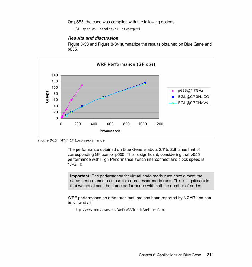
On p655, the code was compiled with the following options:

-O3 -qstrict -qarch=pwr4 -qtune=pwr4

Results and discussionFigure 8-33 and Figure 8-34 summarize the results obtained on Blue Gene and p655.

Figure 8-33 WRF GFLops performance

The performance obtained on Blue Gene is about 2.7 to 2.8 times that of corresponding GFlops for p655. This is significant, considering that p655 performance with High Performance switch interconnect and clock speed is 1.7GHz.

WRF performance on other architectures has been reported by NCAR and can be viewed at:

http://www.mmm.ucar.edu/wrf/WG2/bench/wrf-perf.bmp

WRF Performance (GFlops)

020

40

6080

100120

140

0 200 400 600 800 1000 1200

Processors

GFl

ops [email protected]

BG/[email protected] CO

BG/[email protected] VN

Important: The performance for virtual node mode runs gave almost the same performance as those for coprocessor mode runs. This is significant in that we get almost the same performance with half the number of nodes.


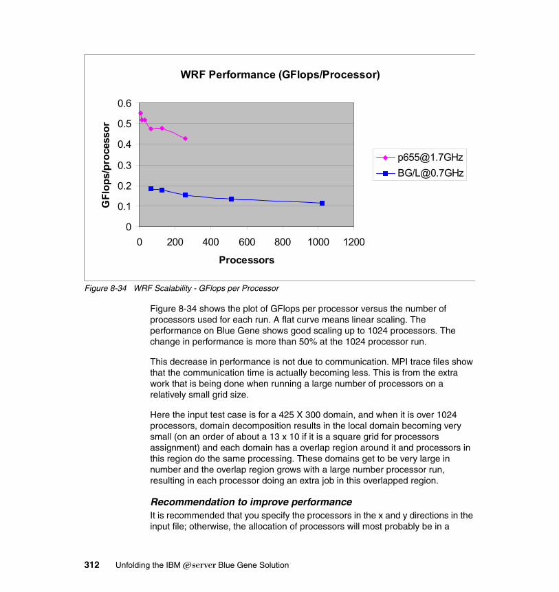
Figure 8-34 WRF Scalability - GFlops per Processor

Figure 8-34 shows the plot of GFlops per processor versus the number of processors used for each run. A flat curve means linear scaling. The performance on Blue Gene shows good scaling up to 1024 processors. The change in performance is more than 50% at the 1024 processor run.

This decrease in performance is not due to communication. MPI trace files show that the communication time is actually becoming less. This is from the extra work that is being done when running a large number of processors on a relatively small grid size.

Here the input test case is for a 425 X 300 domain, and when it is over 1024 processors, domain decomposition results in the local domain becoming very small (on an order of about a 13 x 10 if it is a square grid for processors assignment) and each domain has a overlap region around it and processors in this region do the same processing. These domains get to be very large in number and the overlap region grows with a large number processor run, resulting in each processor doing an extra job in this overlapped region.

Recommendation to improve performanceIt is recommended that you specify the processors in the x and y directions in the input file; otherwise, the allocation of processors will most probably be in a

WRF Performance (GFlops/Processor)

0

0.1

0.2

0.3

0.4

0.5

0.6

0 200 400 600 800 1000 1200

Processors

GFl

ops/

proc

esso

r

[email protected]/[email protected]


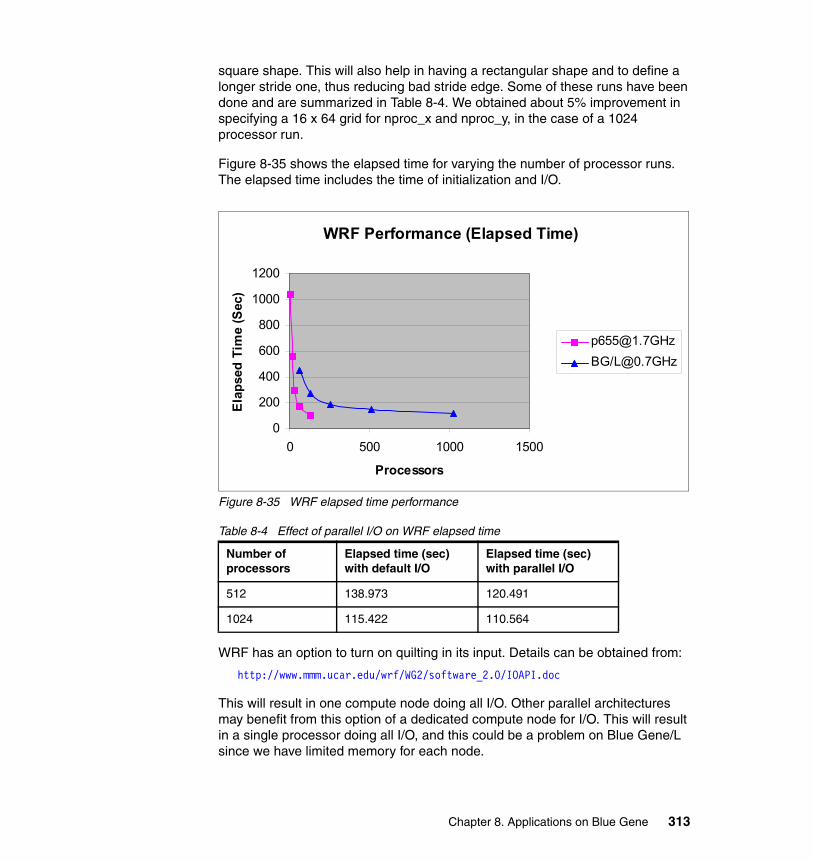
square shape. This will also help in having a rectangular shape and to define a longer stride one, thus reducing bad stride edge. Some of these runs have been done and are summarized in Table 8-4. We obtained about 5% improvement in specifying a 16 x 64 grid for nproc_x and nproc_y, in the case of a 1024 processor run.

Figure 8-35 shows the elapsed time for varying the number of processor runs. The elapsed time includes the time of initialization and I/O.

Figure 8-35 WRF elapsed time performance

Table 8-4 Effect of parallel I/O on WRF elapsed time

WRF has an option to turn on quilting in its input. Details can be obtained from:

http://www.mmm.ucar.edu/wrf/WG2/software_2.0/IOAPI.doc

This will result in one compute node doing all I/O. Other parallel architectures may benefit from this option of a dedicated compute node for I/O. This will result in a single processor doing all I/O, and this could be a problem on Blue Gene/L since we have limited memory for each node.


Elapsed time (sec) with default I/O

Elapsed time (sec) with parallel I/O

512 138.973 120.491

1024 115.422 110.564

WRF Performance (Elapsed Time)

0

200

400

600

800

1000

1200

0 500 1000 1500

Processors

Elap

sed

Tim

e (S

ec)

[email protected]/[email protected]


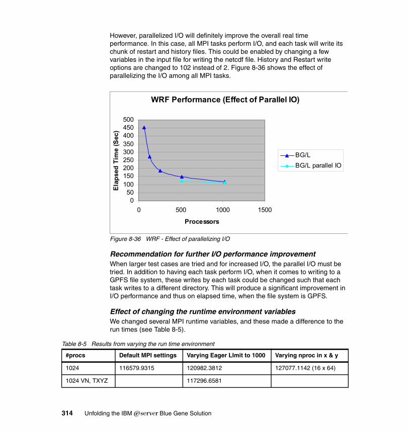
However, parallelized I/O will definitely improve the overall real time performance. In this case, all MPI tasks perform I/O, and each task will write its chunk of restart and history files. This could be enabled by changing a few variables in the input file for writing the netcdf file. History and Restart write options are changed to 102 instead of 2. Figure 8-36 shows the effect of parallelizing the I/O among all MPI tasks.

Figure 8-36 WRF - Effect of parallelizing I/O

Recommendation for further I/O performance improvementWhen larger test cases are tried and for increased I/O, the parallel I/O must be tried. In addition to having each task perform I/O, when it comes to writing to a GPFS file system, these writes by each task could be changed such that each task writes to a different directory. This will produce a significant improvement in I/O performance and thus on elapsed time, when the file system is GPFS.

Effect of changing the runtime environment variablesWe changed several MPI runtime variables, and these made a difference to the run times (see Table 8-5).

Table 8-5 Results from varying the run time environment

WRF Performance (Effect of Parallel IO)

050

100150200250300350400450500

0 500 1000 1500

Processors

Elap

sed

Tim

e (S

ec)

BG/LBG/L parallel IO

#procs Default MPI settings Varying Eager LImit to 1000 Varying nproc in x & y

1024 116579.9315 120982.3812 127077.1142 (16 x 64)

1024 VN, TXYZ 117296.6581


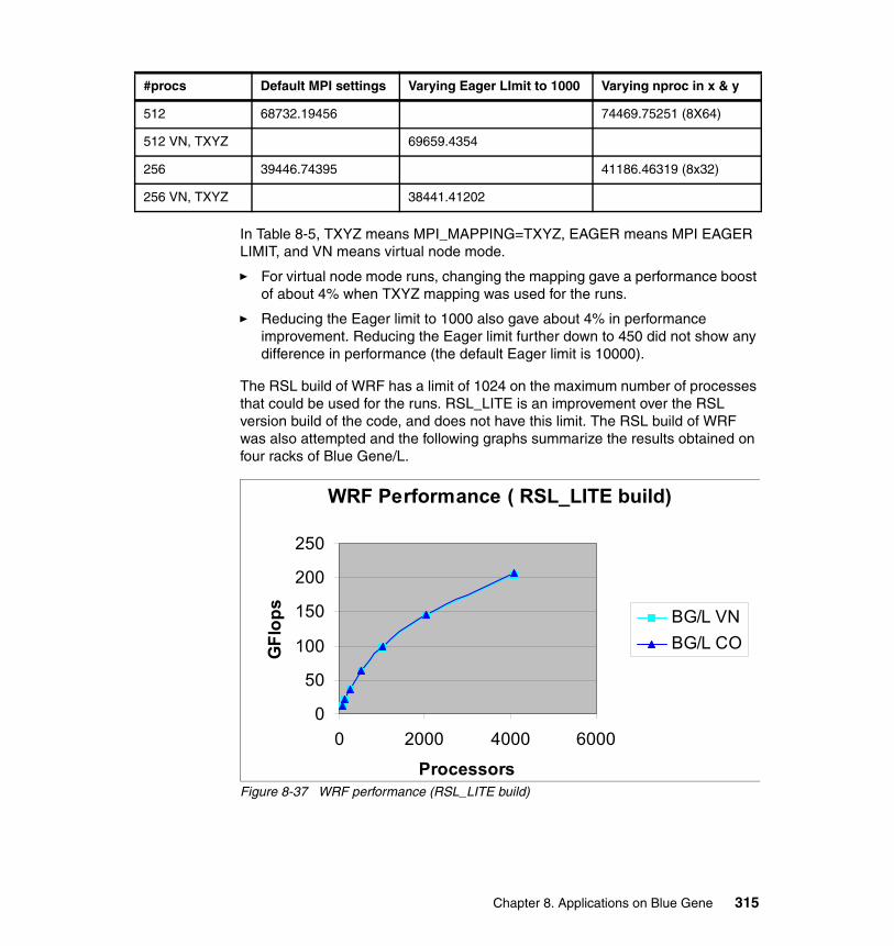
In Table 8-5, TXYZ means MPI_MAPPING=TXYZ, EAGER means MPI EAGER LIMIT, and VN means virtual node mode.

� For virtual node mode runs, changing the mapping gave a performance boost of about 4% when TXYZ mapping was used for the runs.

� Reducing the Eager limit to 1000 also gave about 4% in performance improvement. Reducing the Eager limit further down to 450 did not show any difference in performance (the default Eager limit is 10000).

The RSL build of WRF has a limit of 1024 on the maximum number of processes that could be used for the runs. RSL_LITE is an improvement over the RSL version build of the code, and does not have this limit. The RSL build of WRF was also attempted and the following graphs summarize the results obtained on four racks of Blue Gene/L.

Figure 8-37 WRF performance (RSL_LITE build)

512 68732.19456 74469.75251 (8X64)

512 VN, TXYZ 69659.4354

256 39446.74395 41186.46319 (8x32)

256 VN, TXYZ 38441.41202

#procs Default MPI settings Varying Eager LImit to 1000 Varying nproc in x & y

WRF Performance ( RSL_LITE build)

0

50

100

150

200

250

0 2000 4000 6000

Processors

GFl

ops

BG/L VNBG/L CO


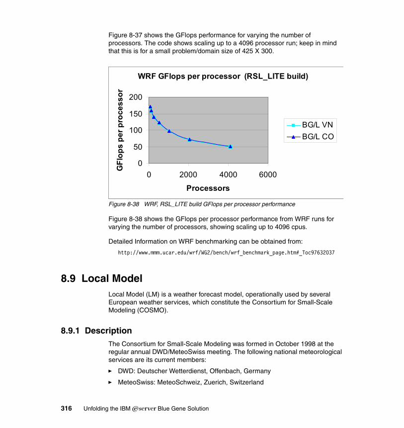
Figure 8-37 shows the GFlops performance for varying the number of processors. The code shows scaling up to a 4096 processor run; keep in mind that this is for a small problem/domain size of 425 X 300.

Figure 8-38 WRF, RSL_LITE build GFlops per processor performance

Figure 8-38 shows the GFlops per processor performance from WRF runs for varying the number of processors, showing scaling up to 4096 cpus.

Detailed Information on WRF benchmarking can be obtained from:

http://www.mmm.ucar.edu/wrf/WG2/bench/wrf_benchmark_page.htm#_Toc97632037

8.9 Local ModelLocal Model (LM) is a weather forecast model, operationally used by several European weather services, which constitute the Consortium for Small-Scale Modeling (COSMO).

8.9.1 DescriptionThe Consortium for Small-Scale Modeling was formed in October 1998 at the regular annual DWD/MeteoSwiss meeting. The following national meteorological services are its current members:

� DWD: Deutscher Wetterdienst, Offenbach, Germany

� MeteoSwiss: MeteoSchweiz, Zuerich, Switzerland

WRF GFlops per processor (RSL_LITE build)

0

50

100

150

200

0 2000 4000 6000

Processors

GFl

ops

per p

roce

ssor

BG/L VNBG/L CO


� UGM: Ufficio Generale per la Meteorologia, Roma®, Italy

� HNMS: the Hellenic National Meteorological Service, Athens, Greece

� IMGW: the Institute of Meteorology and Water Management, Warsaw, Poland

Additionally, the following regional and military services within the member states are participating:

� ARPA-SMR: il Servizio Meteorologico Regionale di ARPA, Bologna, Italy

� AWGeophys: Amt fuer Wehrgeophysik, Traben-Trarbach, Germany

The principal objective of COSMO is the creation of a meso-to-micro scale prediction and simulation system. This system, with LM as its basic model component, is intended to be used as a flexible tool for specific tasks of weather services as well as for various scientific applications on a broad range of spatial scales.

Current operational NWP-models operate on the hydrostatic scales of motion with grid spacings down to about 15 km. Thus, they lack the spatial resolution required to capture explicitly all small-scale, short-duration severe weather events and significant flow systems, which are related to the non-hydrostatic scales of motion. The LM is designed for just these spatial scales, where non-hydrostatic effects play an essential role.

From a mathematical point of view, LM (as any regional weather forecast model) is an initial boundary value problem. This technical term describes that the initial data are given on the whole computational domain at time step 0, and on the boundary of the computational domain for all subsequent time steps.

As this is a numerical forecast model, time step 0 describes the weather as of today, and the subsequent time steps are in the future. Hence, another forecast model is needed to get the boundary data in the future. In operational weather forecasting, a so-called global model (GME from DWD, IFS from ECMWF) provides this information. A global model predicts for the whole globe, hence there are no boundaries to take care of. However, the global model uses only a coarse grid. Therefore, the Local Model is still needed to provide the fine-grained weather information.

The benchmark that was actually run on the Blue Gene/L system was LM_RAPS_3.0, which consists of a subset of LM version 3.10 of the COSMO consortium and the interpolation program INT2LM, which interpolates data from a coarse grid model (GME from DWD, IFS from ECMWF or a coarse grid LM) to the (fine) LM-grid.

Both programs are parallelized for computers with distributed memory using the Message Passing Interface (MPI) as a parallel library. The main interest of the


benchmark focuses on the LM. In the RAPS benchmark, INT2LM is only a utility program to create the necessary LM initial and boundary data on a fine grid.

The initial data provided is the output of a GME global forecast for March 1, 2004, starting at 12:00 UTC for 12 hours on a grid with a 60km mesh size. The interpolation routine INT2LM restricts these data and interpolates them to a finer grid with a mesh size of 7km, covering a rectangular subset of Europe. LM forecasts the weather for March 1, 2004, 12:00-24:00 UTC in the interior of this subset of Europe.

8.9.2 CharacteristicsAs mentioned before, LM_RAPS_3.0 operates on a rectangular subset of Europe. The parallelization is done by further subdividing this rectangular subset both in an East-West and in a North-South direction. This leads to a two-dimensional array of smaller rectangles. Each MPI task takes care of one of these sub-domains.

As with most other local area models, each time step divides into a so-called dynamics and a so-called physics part as described here:

� The dynamics part models the fluid dynamics of the air (computation of wind speed and direction) and the transport (advection) of the other observables like temperature and humidity with the wind. This includes the computation of various differences, with the operands sometimes residing in the memory of different, but neighboring, MPI tasks. The latter is handled in the usual way by providing layers of extra memory around each rectangle (sometimes called halo) and exchanging these layers with neighboring MPI tasks when needed.

� The physics part handles various physical processes like radiation (from the sun), reflection of light at the clouds, and precipitation. In the model simplification, all these physical processes deal only with the vertical column above one single point on the earth’s surface. Hence, all corresponding computations stay entirely within one MPI task and little or no communication is need in this part.

At least once per each forecast hour, new initial and boundary dates have to be read in from a file and the resulting forecast of the previous time steps has to be written to disk. Reading and writing are done by one MPI task. Hence there are broadcast, gather, and scatter operations to get the information from and to the other MPI tasks that do not do I/O.

Unlike many other weather forecast codes, LM does not do any FFTs. Hence there is no need for all-to-all MPI communication. The FFTs are usually used for a fast solution of a Helmholtz equation that originates from an implicit time stepping scheme. LM does the time stepping mostly explicitly, using a much


smaller time step (so-called micro-stepping) for the fluid dynamics part to comply with the Courant-Friedrich-Lax condition.

Given the previous reasons, you should expect the MPI communication to be dominated by nearest neighbor exchanges, followed by gather/scatter-like communication patterns. This hypothesis was tested by running comparison runs on a cluster of 8-way p655+ nodes connected with a High Performance Switch.

The MPI communication was timed with a variant of the ACTC tool MP_tracer, which uses the PMPI interface to intercept the MPI calls. For a run on a 10*16 array of sub-domains, the MPI timing data for MPI task 0 (dealing with the sub-domain at the south-west corner) is shown in Example 8-6.

Example 8-6 MPI timing data for MPI task 0

----------------------------------------------------------MPI Routine #calls avg. bytes time(sec)----------------------------------------------------------MPI_Comm_size 1305 0.0 0.004MPI_Comm_rank 212 0.0 0.000MPI_Send 8694 406394.7 2.555MPI_Recv 16896 367888.0 3.998MPI_Sendrecv 51876 123767.7 191.401MPI_Probe 10494 0.0 2.572MPI_Waitall 1 0.0 0.000MPI_Bcast 4467 53.5 3.987MPI_Barrier 314 0.0 0.410MPI_Gather 7274 12620.6 10.181MPI_Scatter 4071 12780.0 1.672MPI_Allgather 29 4.0 0.070MPI_Reduce 219 71.9 3.489MPI_Allreduce 1125 315.3 26.432----------------------------------------------------------total communication time = 246.770 seconds.total elapsed time = 1285.903 seconds.user cpu time = 1239.480 seconds.system time = 22.420 seconds.maximum memory size = 279284 KBytes.

The data in this example clearly shows that the bulk of the communication time is going into MPI_Sendrecv, which is handling the nearest neighbor exchanges. Except for some MPI_Sends and MPI_Recvs with very large messages (which are part of the I/O part), the remaining communication pattern is tree-based algorithms (MPI_Bcast, MPI_Gather, MPI_Scatter, MPI_Allgather, MPI_Reduce and MPI_Allreduce).


With these tree-based communication patterns expected to run well on the tree network from BG/L, and the nearest neighbor exchanges being well suited for the torus network, LM looked like an almost ideal candidate for porting to BG/L.

8.9.3 Planning for LMGiven the situation as detailed, few problems were expected for the port and the execution performance. The application is already MPI parallel, with a communication profile that can be expected to be well suited for BG/L.

Only the I/O part gave rise to some consideration, since the only available file system on the benchmark system was NFS-mounted. Also, collecting the output on one MPI task and doing a serial I/O from this task clearly will become a performance inhibitor for large numbers of MPI tasks.

But the I/O part contains not only the actual I/O operation, but also translation to and from a special binary output format called GRIB format. GRIB is a standard from the World Meteorological Organization (WMO), which is a United Nations specialized agency. This translation cannot be easily parallelized, so the I/O part was left as is.

8.9.4 Porting experienceLM is available on several platforms, including AIX and Linux. Porting LM to BG/L proved to be mainly a mix-and-match of AIX and Linux features, in exactly the same way as for a port to Linux on Power.

The first step in porting LM was to port the GRIB library that is doing the I/O and the handling of the GRIB format. This library is written partly in C and partly in FORTRAN. So the porting had to cover inter-language calls from FORTRAN to C. This was essentially done by adding the bolded lines (marked with +) to the file lm_raps_3.0/grib1_new/include/fortran_c.h (see Example 8-7).

Example 8-7 Modifying the definition for BG/L

#ifdef __linux__# undef FORTRAN_UPPERCASE# define FORTRAN_UNDERLINE

#endif+#ifdef __plinux__+ # undef FORTRAN_UNDERLINE+ # undef FORTRAN_UPPERCASE+#endif#ifdef _CRAY

# undef FORTRAN_UNDERLINE # define FORTRAN_UPPERCASE


#endif#ifdef _AIX

# undef FORTRAN_UNDERLINE # undef FORTRAN_UPPERCASE

#endif

In other words, a __plinux__ flavor was added, which took the same contents as the _AIX flavor. It was called __plinux__ so it would be the same for a port to Linux on Power. Of course -WF,-D_AIX had to be replaced by -WF,-D__plinux__ for the FORTRAN compiler flags, and a similar change was made for C.

In several places in the code, a defined(__plinux__) had to be added where appropriate, as in the Example 8-8.

Example 8-8 Modifying the source code for __plinux__ awareness

#if defined(_AIX) #include <sys/statvfs.h> #define FSTYPSZ 16! #elif defined(__linux__) || defined(__plinux__) #include <sys/vfs.h> #else #include <sys/fstyp.h> #endif

Note that here, and for other situations dependent on the operating system (as opposed to dependency on xl compilers), __plinux__ takes the same branch as __linux__.

There was one (transient) code addition. In the early stage, the I/O implementation of BG/L was not complete and a statfs was missing. So a dummy statfs was added (Example 8-9) to the GRIB library, which occasionally prints a reminder that it should be removed when no longer needed.

Example 8-9 Workaround for missing statfs() in BG/L

/* this is a work around for a missing statfs function on BG/L */

int dummy_statfs_use_counter = 0;

int statfs (const char *__file, struct statfs *__buf) { __buf->f_type = 0x6969; /* we are only using NFS mounted files */ if ( !(++dummy_statfs_use_counter % 10) ) { fprintf(stderr,

"This is a reminder that there is a work around for statfs\n"); } return(0);


}

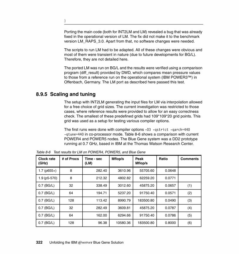
Porting the main code (both for INT2LM and LM) revealed a bug that was already fixed in the operational version of LM. The fix did not make it to the benchmark version LM_RAPS_3.0. Apart from that, no software changes were needed.

The scripts to run LM had to be adapted. All of these changes were obvious and most of them were transient in nature (due to future developments for BG/L). Therefore, they are not detailed here.

The ported LM was run on BG/L and the results were verified using a comparison program (diff_result) provided by DWD, which compares mean pressure values to those from a reference run on the operational system (IBM POWER3™) in Offenbach, Germany. The LM port as described here passed this test.

8.9.5 Scaling and tuningThe setup with INT2LM generating the input files for LM via interpolation allowed for a free choice of grid sizes. The current investigation was restricted to those cases, where reference results were provided to allow for an easy correctness check. The smallest of these predefined grids had 109*109*20 grid points. This grid was used as a setup for testing various compiler options.

The first runs were done with compiler options -O3 -qstrict -qarch=440 -qtune=440 in co-processor mode. Table 8-6 shows a comparison with current POWER4 and POWER5 nodes. The Blue Gene system was a DD2 prototype running at 0.7 GHz, based in IBM at the Thomas Watson Research Center.

Table 8-6 Test results for LM on POWER4, POWER5, and Blue Gene

Clock rate(GHz)

# of Procs Time - sec (LM)

Mflop/s Peak Mflop/s

Ratio Comments

1.7 (p655+) 8 282.40 3610.96 55705.60 0.0648

1.9 (p5-570) 8 212.32 4802.82 62259.20 0.0771

0.7 (BG/L) 32 338.49 3012.60 45875.20 0.0657 (1)

0.7 (BG/L) 64 194.71 5237.20 91750.40 0.0571 (2)

0.7 (BG/L) 128 113.42 8990.79 183500.80 0.0490 (3)

0.7 (BG/L) 32 282.49 3609.81 45875.20 0.0787 (4)

0.7 (BG/L) 64 162.00 6294.66 91750.40 0.0786 (5)

0.7 (BG/L) 128 96.38 10580.36 183500.80 0.8000 (6)


Comments:1. without libmass, -qarch=4402. without libmass, -qarch=4403. without libmass, -qarch=4404. with libmass, -qarch=4405. with libmass, -qarch=4406. with libmass, -qarch=440

Restricting the optimization to -O3 -qstrict is expected to downgrade the performance. This decision was taken based on experience from the customer DWD. Executables generated with optimization level -O5 were found to be only a few percentage points faster, but sometimes produced wrong results.

The Mflop/s rate was measured on POWER4 with a hardware performance monitor (the ACTC tool hpmcount). On POWER5 and Blue Gene, it was assumed that the same number of floating point operations were performed and the POWER4 Mflop/s rate was extrapolated by multiplication with the ratio of execution times.

The peak performance on POWER4 and POWER5 was simply four times the clock rate, assuming that the performance cannot be faster than with both floating point units executing an FMA instruction. With the execution pipeline properly filled, each FMA produces one result per cycle, which is the result of two floating point operations, a multiply operation and an add operation. Two floating point units, each executing two operations at every cycle, provide four flops per cycle, hence the factor four.

The peak performance for Blue Gene in Table 8-6 takes into account that the application is run in co-processor mode. Hence, only one CPU is doing actual computations. Also, -q440 prevents the use of the double floating point unit. So the peak performance per CPU was taken to be only twice the clock rate.

Given this definition of the peak performance, LM operates at roughly the same percentage of the peak performance as on POWER4 and POWER5.

Table 8-6 also shows that the mass lib is giving a significant performance boost. It should be noted that the POWER4 and POWER5 numbers include the corresponding version of the mass lib. Therefore, a fair comparison should compare the POWER4 and POWER5 number to the timings with use of the mass lib.

Employing the double floating point unit proved to be a complicated task. The best result was obtained by compiling just one subroutine (turb_diff) with -qhot -qarch=440d. This routine is known to account for 10% to 20% of the total time (depending on the grid size). This routine is also far from being a simple kernel. It is therefore a challenging task to look at the assembly output or to apply single


node tuning techniques as outlined earlier. The improvement was about 1% of the total execution time.

The grid size of 109*109*20 can be only considered as a test grid. More runs were performed for a grid with size 325*325*35 (using a 7km mesh). A grid like this is currently used in production mode.

Again, the runs on Blue Gene/L were done in co-processor mode and using compiler options -O3 -qstrict -qarch=440 -qtune=440 globally for the whole code.

Figure 8-39 shows the comparison of wall clock times between Blue Gene and the p655+ system at Poughkeepsie. Of course the p655+ system shows a better per node performance based on the higher clock speed of the single CPU. The Blue Gene/L timings are additionally distorted by a weak performance of the I/O part of the program.

Figure 8-39 BG/L execution time

To demonstrate this, Figure 8-39 shows another curve with the same runs, but with the wall clock time being reduced by the time spent in I/O operation. Comparing these two curves shows the effect of I/O on total performance.

Two reasons can be made responsible for the remarkable influence of I/O on the performance numbers. On the one hand there is the limited performance of the NFS server on the benchmark system. Of course this is a transient effect, as the Watson Prototype awaits the implementation of a proper GPFS file system that


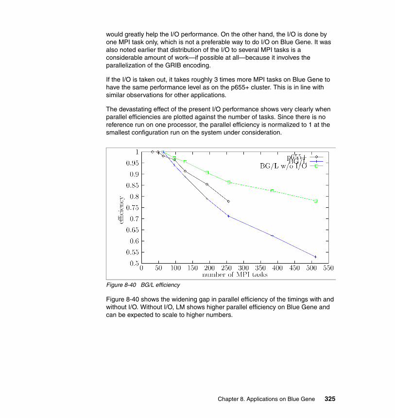
would greatly help the I/O performance. On the other hand, the I/O is done by one MPI task only, which is not a preferable way to do I/O on Blue Gene. It was also noted earlier that distribution of the I/O to several MPI tasks is a considerable amount of work—if possible at all—because it involves the parallelization of the GRIB encoding.

If the I/O is taken out, it takes roughly 3 times more MPI tasks on Blue Gene to have the same performance level as on the p655+ cluster. This is in line with similar observations for other applications.

The devastating effect of the present I/O performance shows very clearly when parallel efficiencies are plotted against the number of tasks. Since there is no reference run on one processor, the parallel efficiency is normalized to 1 at the smallest configuration run on the system under consideration.

Figure 8-40 BG/L efficiency

Figure 8-40 shows the widening gap in parallel efficiency of the timings with and without I/O. Without I/O, LM shows higher parallel efficiency on Blue Gene and can be expected to scale to higher numbers.



Part 4 Appendixes

Part 4



Appendix A. BG/L prior to porting code

When considering whether an application should be ported to the BG/L system, certain technical issues have to be checked. The effort required to port a code to any new hardware should never be underestimated. Therefore, the following list is designed to help in the decision process.

1. Is the code single threaded? The BG/L system does not support thread spawning. Also, have you ensured that scripts are not being used to maintain the workflow?

2. Is the application addressing 32-bit?

3. Does the code use MPI, specifically MPICH v1.2? Although there are many parallel programming APIs, the only one supported by BG/L is MPICH.

4. Is the code SPMD, and not MPMD? The BG/L system only supports the SPMD, same program everywhere, style of parallel programming.

5. Is the memory requirement per MPI task less than 500 MB?

6. Is the code computational-intensive? That is, is there a small amount of I/O compared to computation?

7. Is the code floating point-intensive? This allows the double floating point capability of BG/L to be exploited.

A

Note: Forks, processes, and threads are not supported on BG/L.


8. Have you ensured that the code does not use flex_lm licensing? At present, there is no flex_lm library support for pLinux.

If you have answered all of the above with yes, then the next questions are:

� Has the code been ported to pLinux?

� Can the problem size be increased with increased numbers of processors?

� Do you use standard input? If yes, can this be changed to a single file input?


Appendix B. BG/L runtime system calls

While the majority of the Blue Gene/L runtime system (called blrts or RTS) is not exposed to the end user, there are several functions in the RTS which can be useful to the application programmer. They are summarized in this appendix.

The runtime system calls are externalized through a library, librts.rts.a, which can be found in the BG/L system library directory. If you want to use the RTS function calls, you need to link with this library:

blrts_xlf90 ... -L /bgl/BlueLight/ppcfloor/bglsys/lib -l rts.rts ...

The function interfaces and data structures are documented via C/C++ language header files. These header files can be found in the BG/L system include directory. To include them in your C or C++ application, make sure that this directory is in your include path:

blrts_xlc ... -I /bgl/BlueLight/ppcfloor/bglsys/include ...

In the following sections we present useful function calls that are declared in the rts.h header. We also explain the details of the Blue Gene/L nodes’ personality, which can be found in the bglpersonality.h header.

Then we show examples of how to access this information from FORTRAN programs. The wrapper code that we created to make these runtime functions available to FORTRAN are provided in the Additional Materials section of the redbooks Web site:


B


B.1 Calls in rts.hThis header contains the declarations for the external functions in the rts.rts library. Three of them are interesting for general use:

The rts_get_timebase() function can be used for timing purposes:

/* Access hardware timebase registers. Taken: nothing Returned: number of processor cycles executed since boot*/unsigned long long rts_get_timebase();

This number of clock ticks can be converted to seconds using the processor speed (clockHz) that is part of the BGLpersonality; this is explained in the next section.

The rts_get_processor() function can be used to find out if the process runs on the first CPU or second CPU of a node. This is the fourth dimension T (in addition to torus coordinates X, Y and Z) when running in virtual node mode:

/* Get processor id. Taken: nothing Returned: 0="I am main processor", 1="I am coprocessor"*/extern int rts_get_processor_id();

The rts_get_personality() function is used to access the Blue Gene/L personality data structure. This is described in detail in the following section, and rts.h actually includes bglpersonality.h to access the declaration of this structure:

/* Obtain chip personality information. Taken: place to put information size of that area Returned: 0=success

non-0=failure (errno gives reason)*/#include <bglpersonality.h>extern int rts_get_personality(BGLPersonality *dst, unsigned size);

When you call this function, you provide the address of a BGLpersonality structure as the first argument and the size of that variable as the second:

#include <rts.h>;BGLPersonality personality;rts_get_personality(&personality, sizeof(personality));

Most of the other functions in rts.h explicitly deal with the coordination between the two CPUs on the chip and will not be used directly by application programs.


B.2 Personality data in bglpersonality.hThe personality of a Blue Gene/L node is static data given to every compute node and I/O node at boot time by the control system. This data contains information specific to the node, with respect to the block that is being booted.

BGLPersonality is a C language typedef for a structure which contains items like the node’s coordinates on the torus network. This kind of information can be very useful if the application programmer wants to determine at runtime where the tasks of the application are actually running. It can also be used to tune certain aspects of the application at runtime, like finding out which set of tasks share the same I/O node and then optimizing the network traffic from the compute nodes to that I/O node.

Here is an excerpt from the structure declaration:

typedef struct BGLPersonality {uint16_t CRC; /* CRC for verification */uint8_t personalitySize; /* Size of struct in 4-byte words */uint8_t version; /* BGLPERSONALITY_VERSION */uint32_t DDRSize; /* Memory size in bytes */...uint32_t clockHz; /* Clock base frequency in Hz */...int8_t xCoord; /* X coord of this node in torus (-1 for I/O node) */int8_t yCoord; /* Y coord of this node in torus (-1 for I/O node) */int8_t zCoord; /* Z coord of this node in torus (-1 for I/O node) */...

inline unsigned getVersion() const;...

}

The last line shows a C++ style access function declaration. Using this is a more portable alternative to referencing the structure components directly. Similar functions exist for the other structure components, and they are implemented further down in the header file. For example:

inline unsigned BGLPersonality::getVersion() const { return this->version; }

For C, there are static inline functions which serve the same purpose:

/* return X coordinate of this node */static inline unsigned BGLPersonality_xCoord(const BGLPersonality *p){ return p->xCoord;}

Appendix B. BG/L runtime system calls 333

Note that the header file also contains functions to set some of these values. These should never be invoked by an application, but only by the control system when bringing up the node.

B.2.1 The sanity.c exampleIn Example B-1 we show a short C program that we found very useful to run on Blue Gene/L partitions as a basic health check. It prints the MPI task information, the task’s location on the torus network, the physical location code of the compute node it is executing on, and its pset membership. A processor set or pset is the group of compute nodes that are controlled by a single I/O node. There may be one or more psets in a partition, and understanding the pset relationships may be useful for tuning purposes.

Example: B-1 The sanity.c health check program

#include <stdio.h>#include <mpi.h>#include <rts.h>#include <bglpersonality.h>

int main (int argc, char **argv){ int num_procs, my_rank; char location[BGLPERSONALITY_MAX_LOCATION]; BGLPersonality personality;

MPI_Init(&argc, &argv); MPI_Comm_size(MPI_COMM_WORLD, &num_procs); MPI_Comm_rank(MPI_COMM_WORLD, &my_rank);

/* BlueGene runtime: get personality */ rts_get_personality(&personality, sizeof(personality)); BGLPersonality_getLocationString(&personality, location);

Attention: The bglpersonality.h data structures have changed several times as new drivers were released, and may change in the future. It is necessary to recompile your application if such changes happen. As a safety check, you can inspect the following:

� The BGLPersonality structure has a component named version which can be checked at runtime, for example through an assert statement.

� The header itself has a #define with a version number in it:

#define BGLPERSONALITY_VERSION 11

If any of this changes, a recompile may be a good idea.


if ( my_rank == 0 ) { printf("-----------------------------------------------------------------------\n"); printf("T: MPI-R/S TORUS-MYCOORD/SIZE TORUS VN? MEMORY LOCATION\n"); printf("P: MPI-R/S PSET-NUM PSET-COORD/SIZE/ORIGIN GI? LOCATION\n"); printf("-----------------------------------------------------------------------\n"); }

/* print my MPI and torus coordinates, plus physical location */ printf("T: %04d/%d <%d,%d,%d,%d>/<%d,%d,%d,%d> %1d%1d%1d %2s %3dMB(%d) %s\n",

my_rank, num_procs, BGLPersonality_xCoord(&personality), BGLPersonality_yCoord(&personality), BGLPersonality_zCoord(&personality),

rts_get_processor_id(), BGLPersonality_xSize(&personality), BGLPersonality_ySize(&personality), BGLPersonality_zSize(&personality), BGLPersonality_virtualNodeMode(&personality)+1, BGLPersonality_isTorusX(&personality), BGLPersonality_isTorusY(&personality), BGLPersonality_isTorusZ(&personality), BGLPersonality_virtualNodeMode(&personality) ? "VN" : "CO", BGLPersonality_DDRSize(&personality)/(1024*1024), personality.DDRModuleType, location);

/* print my MPI and pset coordinates, plus physical location */ printf("P: %04d/%d %03d/%d/%d/%d <%d,%d,%d>/<%d,%d,%d>/<%d,%d,%d> %1d %s\n",

my_rank, num_procs,

BGLPersonality_rankInPset(&personality), BGLPersonality_numNodesInPset(&personality), BGLPersonality_psetNum(&personality), BGLPersonality_numPsets(&personality),

BGLPersonality_xPsetCoord(&personality), BGLPersonality_yPsetCoord(&personality), BGLPersonality_zPsetCoord(&personality), BGLPersonality_xPsetSize(&personality), BGLPersonality_yPsetSize(&personality), BGLPersonality_zPsetSize(&personality),


BGLPersonality_xPsetOrigin(&personality), BGLPersonality_yPsetOrigin(&personality), BGLPersonality_zPsetOrigin(&personality),

BGLPersonality_useGlobalInterrupts(&personality),

location );

MPI_Finalize(); exit(0);}

B.2.2 Accessing the BG/L runtime information from FORTRANAccessing the personality data from FORTRAN is not easily possible, since accessing C struct data from FORTRAN is difficult and the accessor functions are inline functions rather than extern functions that can be linked to. Therefore, this section presents some wrapper code that can be used to access personality information from FORTRAN. The RTS function calls themselves are easier to translate into FORTRAN, but for convenience we also provide FORTRAN wrappers for those.

Example B-2 on page 336 shows a FORTRAN module that contains the interface definition of the RTS functions. The same can also be provided as an include file of course. The module uses the BIND(C) attribute and ISO_C_BINDING intrinsic module of FORTRAN2003 to facilitate portable language interoperability. This is a useful new feature in XLF Version 9.

Example: B-2 FORTRAN module RTS

module rtsinterface

function rts_get_timebase() bind(c) use, intrinsic :: iso_c_binding integer(c_long_long) :: rts_get_timebase end function rts_get_timebase

function rts_get_processor_id() bind(c) use, intrinsic :: iso_c_binding integer(c_int) :: rts_get_processor_id end function rts_get_processor_id end interface

end module rts


To access the personality data, we decided to avoid passing around the BGLPersonality structure in FORTRAN, and instead write some C extern functions that do this internally and can then be called from FORTRAN. So there are two steps involved: creating the C extern wrappers, and creating a FORTRAN module (or include file) with the interface definitions.

Example B-3 on page 337 shows the bglpersonality_f.c wrapper. It defines a C extern function for all those inline accessor function in bglpersonality.h that take a BGLPersonality input argument. To make calling from FORTRAN easier, arguments are always passed in by reference and the wrappers use a local BGLPersonality variable and pass that to the inline accessor function. So from FORTRAN, only the remaining arguments need to be specified.

Example: B-3 bglpersonailty_f.c: C extern wrappers for bglpersonality.c

#include "rts.h"#include "bglpersonality.h"

extern unsigned bglpersonality_ddrsize(){ BGLPersonality p; (void)rts_get_personality(&p, sizeof(p)); return BGLPersonality_DDRSize(&p);}...extern void bglpersonality_treeaddr2coords( unsigned *treeaddr, unsigned *x, unsigned *y, unsigned *z)/* unsigned treeaddr, unsigned *x, unsigned *y, unsigned *z */{ BGLPersonality p; (void)rts_get_personality(&p, sizeof(p)); BGLPersonality_treeAddr2Coords(&p, *treeaddr, x, y, z);}...extern void bglpersonality_getlocationstring(char *buf){ BGLPersonality p; (void)rts_get_personality(&p, sizeof(p)); BGLPersonality_getLocationString(&p, buf);}

The FORTRAN module in Example B-4 on page 338 contains the interface blocks for the wrapper functions of Example B-3 on page 337, as well as a constant definition for the maximum length of the location string.


Example: B-4 FORTRAN module BGLPERSONALITY

module bglpersonalityinteger, parameter :: BGLPERSONALITY_MAX_LOCATION = 24

interfacefunction bglpersonality_ddrsize() bind(c)use, intrinsic :: iso_c_binding

integer(c_int) :: bglpersonality_ddrsizeend function bglpersonality_ddrsize

...subroutine bglpersonality_treeaddr2coords(treeaddr,x,y,z) bind(c)use, intrinsic :: iso_c_bindinginteger(c_int), intent(in) :: treeaddrinteger(c_int), intent(out) :: x, y, z

end subroutine bglpersonality_treeaddr2coords...

subroutine bglpersonality_getlocationstring(buf) bind(c)use, intrinsic :: iso_c_bindingcharacter(len=BGLPERSONALITY_MAX_LOCATION), intent(out) :: buf

end subroutine bglpersonality_getlocationstringend interface

end module bglpersonality

To make these wrappers available to all users, put the *.mod files into your local include directory and bundle up the object files for the FORTRAN modules and the bglpersonality_f.c wrappers into a library that you put into your local library directory:

BGLSYS = /bgl/BlueLight/ppcfloor/bglsysCC = /opt/ibmcmp/vac/7.0/bin/blrts_xlcFC = /opt/ibmcmp/xlf/9.1/bin/blrts_xlf90CFLAGS= -O2 -I$(BGLSYS)/include -L$(BGLSYS)/lib

all: librtsfortran.a

librtsfortran.a: rts.o bglpersonality.o bglpersonality_f.oar crvf librtsfortran.a rts.o bglpersonality.o bglpersonality_f.o

bglpersonality_f.o: bglpersonality_f.c Makefile

bglpersonality.o: bglpersonality.f Makefile

rts.o: rts.f Makefile

clean::rm -rf *.a *.o *.mod *~ *core*


All of these source files are available for download, together with the makefile to build the modules and libraries, from:

http://www.redbooks.ibm.com.

B.2.3 Sanity revisited: sanity.f90Example B-5 on page 339 contains a FORTRAN 90 program that prints the same information as the C program in Example B-1 on page 334, using the FORTRAN modules described in the previous section.

Example: B-5 The sanity health check (simplified) program (FORTRAN)

program rts_from_fortran use rts use bglpersonality use, intrinsic :: iso_c_binding implicit none real :: x(10000) integer :: i integer(c_long_long) :: t1, t2 integer(c_int) :: cpu character(len=BGLPERSONALITY_MAX_LOCATION) :: loc

cpu=bglpersonality_clockhz() print *, "cpu=", cpu

call bglpersonality_getlocationstring(loc) print *, "loc ==>", loc, "<=="

t1=rts_get_timebase() do i=1,100000 call random_number(x) end do t2=rts_get_timebase() print *, "t1=", t1, t1/cpu print *, "t2=", t2, t2/cpu print *, "diff=", t2-t1, 1.0d0*(t2-t1)/cpuend program rts_from_fortran



Appendix C. Floating point instruction set

The Blue Gene/L processors are based on the PowerPC 440 processor core, which is a 32-bit RISC processor conforming to the “Book E enhanced PowerPC Architecture” documented at:

http://www.ibm.com/chips/techlib

The instruction set for the PowerPC 440 is included in this public documentation.

The special floating point unit on Blue Gene/L processors implements extra instructions, or “extensions” to the base instruction set architecture.

This appendix provides the mnemonics and meanings for these extra instructions in order to help analysis of assembler listings of code running on the Blue Gene/L system.

These instructions are required because of the SIMD-like double floating point unit. SIMD stands for “single instruction, multiple data” and means that a single instruction can cause both floating point units to perform the same operation at the same time, but with each floating point unit using its own private register set.

In the base architecture, floating point operations apply to a single floating point unit which has 32 floating point registers. On Blue Gene/L, in addition to the base floating point instructions which continue to operate unchanged, additional

C


instructions act on the second floating point unit with its own set of 32 floating point registers.

C.1 Instruction types specific to BG/L PPC440There are three additional instruction types which have been added to the architecture:

1. Parallel instructions, which cause both floating point units to execute the same floating point instruction on data contained in each floating point’s local register set.

2. Cross instructions, which cause both floating point units to execute the same floating point instruction, but in which some of the operands are common to both instructions.

3. Secondary instructions, which cause only the extra, secondary floating point unit to operate, with instructions equivalent to those provided for the primary floating point unit in the base instruction set architecture.

The cross instruction type should be explained further. Some instructions may contain a constant value that is used repeatedly. For example, we may have two identical instructions which we might want to execute in parallel, such as A=BxC and D=ExC. It would be wasteful to have to load the value C twice, once for each separate floating point unit’s register set. A cross instruction allows the specification of a single value in either FPU’s register set and tells both floating point units to use this value.

The other important point is that the result of a cross instruction has to be stored in the register set of the FPU processing the instruction. In other words, it is possible to read the contents of the register on the other FPU, but not to store information into the other FPU’s register set.

The mnemonics for these three instruction types can be identified at a high level by their common features:

1. Parallel instructions for memory load/store operations start with “lfp” or “stfp”.Parallel instructions for other operations start with “fp”.

2. Cross instructions for memory load/store operations start with “lfx” or “stfx”.Cross instructions for other operations start with “fx”.

3. Secondary instructions for memory load/store operations start with “lfs” or “stfs”.Secondary instructions for other operations start with “fs”.


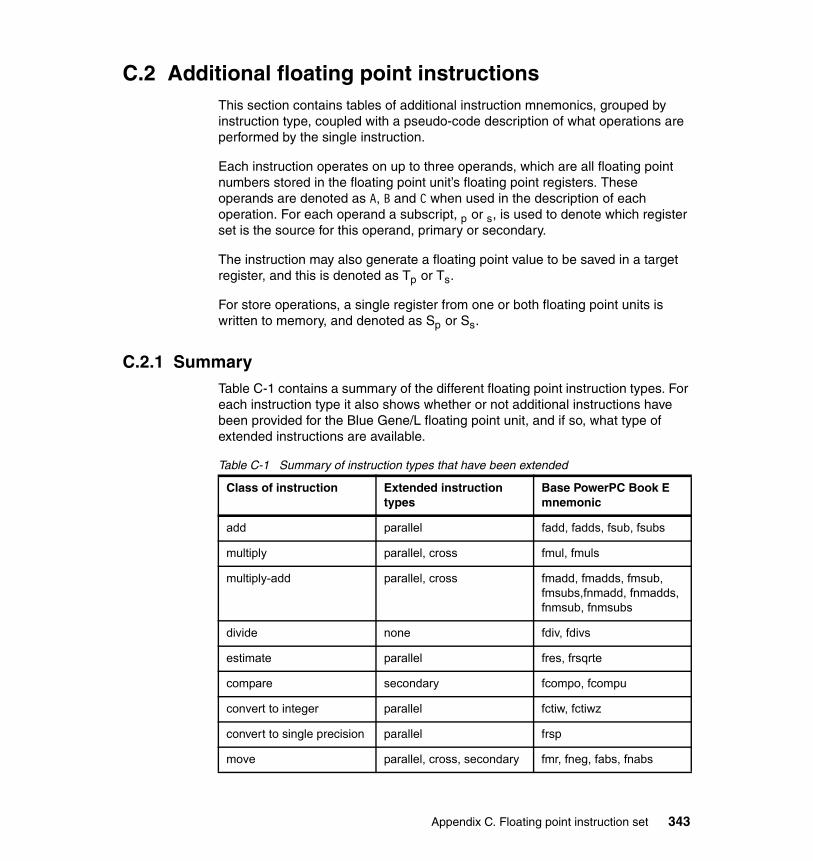
C.2 Additional floating point instructionsThis section contains tables of additional instruction mnemonics, grouped by instruction type, coupled with a pseudo-code description of what operations are performed by the single instruction.

Each instruction operates on up to three operands, which are all floating point numbers stored in the floating point unit’s floating point registers. These operands are denoted as A, B and C when used in the description of each operation. For each operand a subscript, p or s, is used to denote which register set is the source for this operand, primary or secondary.

The instruction may also generate a floating point value to be saved in a target register, and this is denoted as Tp or Ts.

For store operations, a single register from one or both floating point units is written to memory, and denoted as Sp or Ss.

C.2.1 SummaryTable C-1 contains a summary of the different floating point instruction types. For each instruction type it also shows whether or not additional instructions have been provided for the Blue Gene/L floating point unit, and if so, what type of extended instructions are available.

Table C-1 Summary of instruction types that have been extended

Class of instruction Extended instruction types

Base PowerPC Book E mnemonic

add parallel fadd, fadds, fsub, fsubs

multiply parallel, cross fmul, fmuls

multiply-add parallel, cross fmadd, fmadds, fmsub, fmsubs,fnmadd, fnmadds, fnmsub, fnmsubs

divide none fdiv, fdivs

estimate parallel fres, frsqrte

compare secondary fcompo, fcompu

convert to integer parallel fctiw, fctiwz

convert to single precision parallel frsp

move parallel, cross, secondary fmr, fneg, fabs, fnabs

Appendix C. Floating point instruction set 343

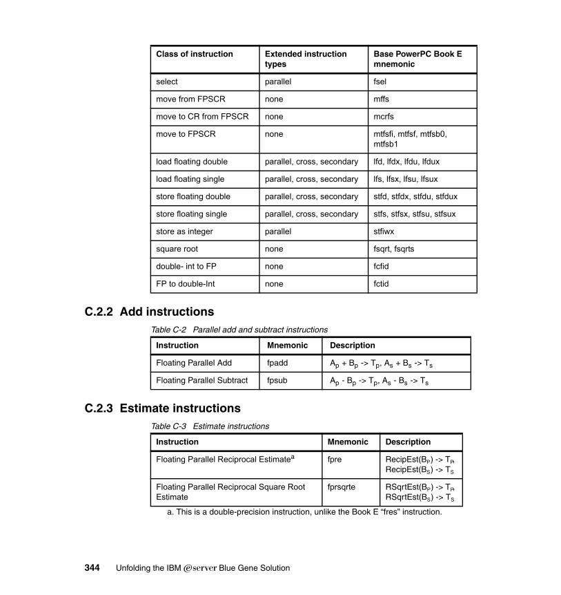
C.2.2 Add instructionsTable C-2 Parallel add and subtract instructions

C.2.3 Estimate instructionsTable C-3 Estimate instructions

select parallel fsel

move from FPSCR none mffs

move to CR from FPSCR none mcrfs

move to FPSCR none mtfsfi, mtfsf, mtfsb0, mtfsb1

load floating double parallel, cross, secondary lfd, lfdx, lfdu, lfdux

load floating single parallel, cross, secondary lfs, lfsx, lfsu, lfsux

store floating double parallel, cross, secondary stfd, stfdx, stfdu, stfdux

store floating single parallel, cross, secondary stfs, stfsx, stfsu, stfsux

store as integer parallel stfiwx

square root none fsqrt, fsqrts

double- int to FP none fcfid

FP to double-Int none fctid

Class of instruction Extended instruction types

Base PowerPC Book E mnemonic

Instruction Mnemonic Description

Floating Parallel Add fpadd Ap + Bp -> Tp, As + Bs -> Ts

Floating Parallel Subtract fpsub Ap - Bp -> Tp, As - Bs -> Ts


Floating Parallel Reciprocal Estimatea

a. This is a double-precision instruction, unlike the Book E “fres” instruction.

fpre RecipEst(BP) -> TP, RecipEst(BS) -> TS

Floating Parallel Reciprocal Square Root Estimate

fprsqrte RSqrtEst(BP) -> TP, RSqrtEst(BS) -> TS


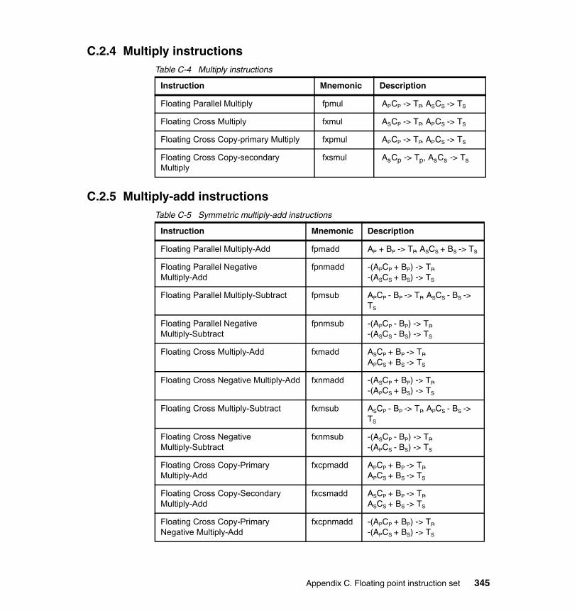
C.2.4 Multiply instructionsTable C-4 Multiply instructions

C.2.5 Multiply-add instructionsTable C-5 Symmetric multiply-add instructions


Floating Parallel Multiply fpmul APCP -> TP, ASCS -> TS

Floating Cross Multiply fxmul ASCP -> TP, APCS -> TS

Floating Cross Copy-primary Multiply fxpmul APCP -> TP, APCS -> TS

Floating Cross Copy-secondary Multiply

fxsmul AsCp -> Tp, AsCs -> Ts


Floating Parallel Multiply-Add fpmadd AP + BP -> TP, ASCS + BS -> TS

Floating Parallel Negative Multiply-Add

fpnmadd -(APCP + BP) -> TP,-(ASCS + BS) -> TS

Floating Parallel Multiply-Subtract fpmsub APCP - BP -> TP, ASCS - BS -> TS

Floating Parallel Negative Multiply-Subtract

fpnmsub -(APCP - BP) -> TP,-(ASCS - BS) -> TS

Floating Cross Multiply-Add fxmadd ASCP + BP -> TP,APCS + BS -> TS

Floating Cross Negative Multiply-Add fxnmadd -(ASCP + BP) -> TP,-(APCS + BS) -> TS

Floating Cross Multiply-Subtract fxmsub ASCP - BP -> TP, APCS - BS -> TS

Floating Cross Negative Multiply-Subtract

fxnmsub -(ASCP - BP) -> TP,-(APCS - BS) -> TS

Floating Cross Copy-Primary Multiply-Add

fxcpmadd APCP + BP -> TP,APCS + BS -> TS

Floating Cross Copy-Secondary Multiply-Add

fxcsmadd ASCP + BP -> TP,ASCS + BS -> TS

Floating Cross Copy-Primary Negative Multiply-Add

fxcpnmadd -(APCP + BP) -> TP,-(APCS + BS) -> TS


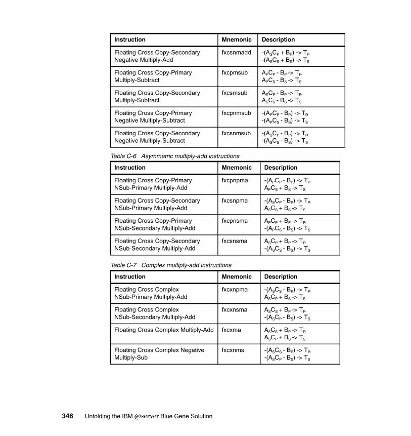
Table C-6 Asymmetric multiply-add instructions

Table C-7 Complex multiply-add instructions

Floating Cross Copy-Secondary Negative Multiply-Add

fxcsnmadd -(ASCP + BP) -> TP,-(ASCS + BS) -> TS

Floating Cross Copy-Primary Multiply-Subtract

fxcpmsub APCP - BP -> TP,APCS - BS -> TS

Floating Cross Copy-Secondary Multiply-Subtract

fxcsmsub ASCP - BP -> TP,ASCS - BS -> TS

Floating Cross Copy-Primary Negative Multiply-Subtract

fxcpnmsub -(APCP - BP) -> TP,-(APCS - BS) -> TS

Floating Cross Copy-Secondary Negative Multiply-Subtract

fxcsnmsub -(ASCP - BP) -> TP,-(ASCS - BS) -> TS


Floating Cross Copy-Primary NSub-Primary Multiply-Add

fxcpnpma -(APCP - BP) -> TP,APCS + BS -> TS

Floating Cross Copy-Secondary NSub-Primary Multiply-Add

fxcsnpma -(ASCP - BP) -> TP,ASCS + BS -> TS

Floating Cross Copy-Primary NSub-Secondary Multiply-Add

fxcpnsma APCP + BP -> TP,-(APCS - BS) -> TS

Floating Cross Copy-Secondary NSub-Secondary Multiply-Add

fxcsnsma ASCP + BP -> TP,-(ASCS - BS) -> TS


Floating Cross Complex NSub-Primary Multiply-Add

fxcxnpma -(ASCS - BP) -> TP,ASCP + BS -> TS

Floating Cross Complex NSub-Secondary Multiply-Add

fxcxnsma ASCS + BP -> TP,-(ASCP - BS) -> TS

Floating Cross Complex Multiply-Add fxcxma ASCS + BP -> TP,ASCP + BS -> TS

Floating Cross Complex Negative Multiply-Sub

fxcxnms -(ASCS - BP) -> TP,-(ASCP - BS) -> TS



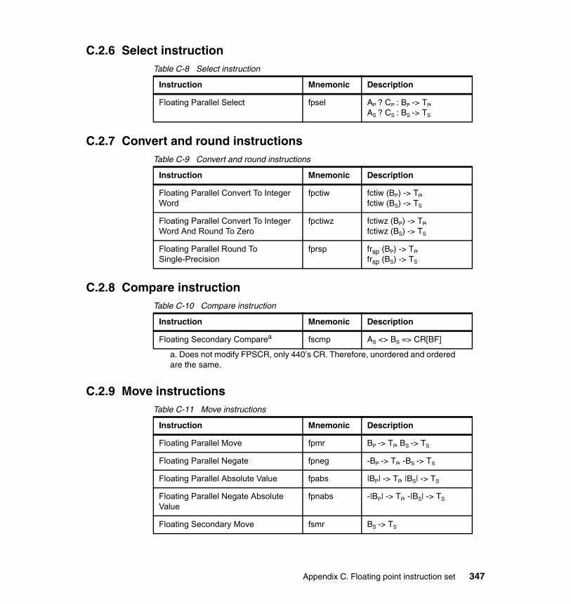
C.2.6 Select instructionTable C-8 Select instruction

C.2.7 Convert and round instructionsTable C-9 Convert and round instructions

C.2.8 Compare instructionTable C-10 Compare instruction

C.2.9 Move instructionsTable C-11 Move instructions


Floating Parallel Select fpsel AP ? CP : BP -> TP,AS ? CS : BS -> TS


Floating Parallel Convert To Integer Word

fpctiw fctiw (BP) -> TP, fctiw (BS) -> TS

Floating Parallel Convert To Integer Word And Round To Zero

fpctiwz fctiwz (BP) -> TP,fctiwz (BS) -> TS

Floating Parallel Round To Single-Precision

fprsp frsp (BP) -> TP,frsp (BS) -> TS


Floating Secondary Comparea

a. Does not modify FPSCR, only 440’s CR. Therefore, unordered and orderedare the same.

fscmp AS <> BS => CR[BF]


Floating Parallel Move fpmr BP -> TP, BS -> TS

Floating Parallel Negate fpneg -BP -> TP, -BS -> TS

Floating Parallel Absolute Value fpabs |BP| -> TP, |BS| -> TS

Floating Parallel Negate Absolute Value

fpnabs -|BP| -> TP, -|BS| -> TS

Floating Secondary Move fsmr BS -> TS


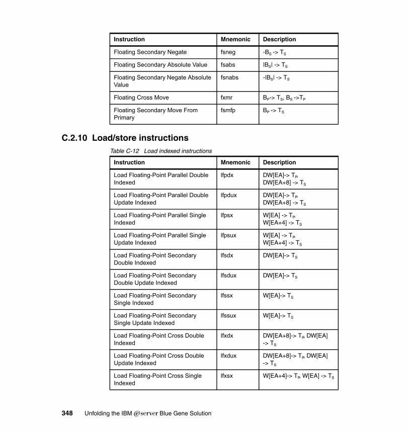
C.2.10 Load/store instructionsTable C-12 Load indexed instructions

Floating Secondary Negate fsneg -BS -> TS

Floating Secondary Absolute Value fsabs |BS| -> TS

Floating Secondary Negate Absolute Value

fsnabs -|BS| -> TS

Floating Cross Move fxmr BP-> TS, BS ->TP

Floating Secondary Move From Primary

fsmfp BP -> TS



Load Floating-Point Parallel Double Indexed

lfpdx DW[EA]-> TP, DW[EA+8] -> TS

Load Floating-Point Parallel Double Update Indexed

lfpdux DW[EA]-> TP, DW[EA+8] -> TS

Load Floating-Point Parallel Single Indexed

lfpsx W[EA] -> TP,

W[EA+4] -> TS

Load Floating-Point Parallel Single Update Indexed

lfpsux W[EA] -> TP,

W[EA+4] -> TS

Load Floating-Point Secondary Double Indexed

lfsdx DW[EA]-> TS

Load Floating-Point Secondary Double Update Indexed

lfsdux DW[EA]-> TS

Load Floating-Point Secondary Single Indexed

lfssx W[EA]-> TS

Load Floating-Point Secondary Single Update Indexed

lfssux W[EA]-> TS

Load Floating-Point Cross Double Indexed

lfxdx DW[EA+8]-> TP, DW[EA] -> TS

Load Floating-Point Cross Double Update Indexed

lfxdux DW[EA+8]-> TP, DW[EA] -> TS

Load Floating-Point Cross Single Indexed

lfxsx W[EA+4]-> TP, W[EA] -> TS


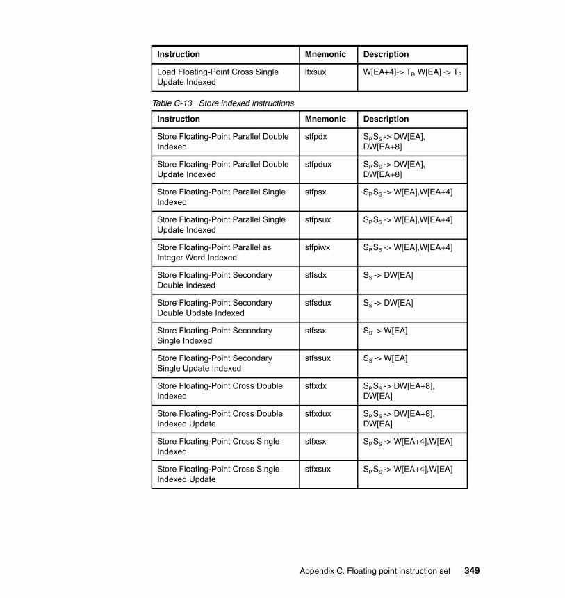
Table C-13 Store indexed instructions

Load Floating-Point Cross Single Update Indexed

lfxsux W[EA+4]-> TP, W[EA] -> TS


Store Floating-Point Parallel Double Indexed

stfpdx SP,SS -> DW[EA], DW[EA+8]

Store Floating-Point Parallel Double Update Indexed

stfpdux SP,SS -> DW[EA], DW[EA+8]

Store Floating-Point Parallel Single Indexed

stfpsx SP,SS -> W[EA],W[EA+4]

Store Floating-Point Parallel Single Update Indexed

stfpsux SP,SS -> W[EA],W[EA+4]

Store Floating-Point Parallel as Integer Word Indexed

stfpiwx SP,SS -> W[EA],W[EA+4]

Store Floating-Point Secondary Double Indexed

stfsdx SS -> DW[EA]

Store Floating-Point Secondary Double Update Indexed

stfsdux SS -> DW[EA]

Store Floating-Point Secondary Single Indexed

stfssx SS -> W[EA]

Store Floating-Point Secondary Single Update Indexed

stfssux SS -> W[EA]

Store Floating-Point Cross Double Indexed

stfxdx SP,SS -> DW[EA+8], DW[EA]

Store Floating-Point Cross Double Indexed Update

stfxdux SP,SS -> DW[EA+8], DW[EA]

Store Floating-Point Cross Single Indexed

stfxsx SP,SS -> W[EA+4],W[EA]

Store Floating-Point Cross Single Indexed Update

stfxsux SP,SS -> W[EA+4],W[EA]




Appendix D. Some useful utilities

The Blue Gene/L system we used for this project provides locally written scripts which are referred to in this redbook, and which may prove useful for other installations.

On the system we used, the scripts are located in the /bgl/console/bin directory, as shown in Example D-1.

Example: D-1 Summary listing

jfollows@bgfe01:/bgl/console/bin> pwd/bgl/console/binjfollows@bgfe01:/bgl/console/bin> ls -rtlatotal 28-rwxr-xr-x 1 500 bgl1 232 2005-01-30 09:22 bglusers-rwxr-xr-x 1 500 bgl1 174 2005-01-30 09:22 bgljobsdrwxrwxr-x 10 500 bgl1 4096 2005-01-30 22:24 ..-rwxr-xr-x 1 500 bgl1 193 2005-02-03 17:43 bglblocks-rwxr-xr-x 1 500 bgl1 344 2005-02-03 18:00 bglconsoledrwxr-xr-x 2 500 bgl1 4096 2005-02-10 18:25 .

Since the scripts are relatively simple DB2 queries, this appendix shows their contents followed by a sample of their output.

D


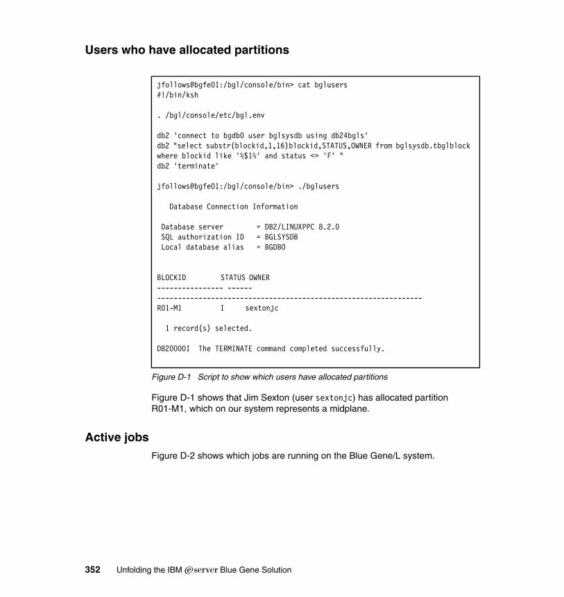
Users who have allocated partitions

Figure D-1 Script to show which users have allocated partitions

Figure D-1 shows that Jim Sexton (user sextonjc) has allocated partition R01-M1, which on our system represents a midplane.

Active jobsFigure D-2 shows which jobs are running on the Blue Gene/L system.

jfollows@bgfe01:/bgl/console/bin> cat bglusers#!/bin/ksh


db2 'connect to bgdb0 user bglsysdb using db24bgls'db2 "select substr(blockid,1,16)blockid,STATUS,OWNER from bglsysdb.tbglblock where blockid like '%$1%' and status <> 'F' "db2 'terminate'

jfollows@bgfe01:/bgl/console/bin> ./bglusers



BLOCKID STATUS OWNER ---------------- ------ ----------------------------------------------------------------R01-M1 I sextonjc




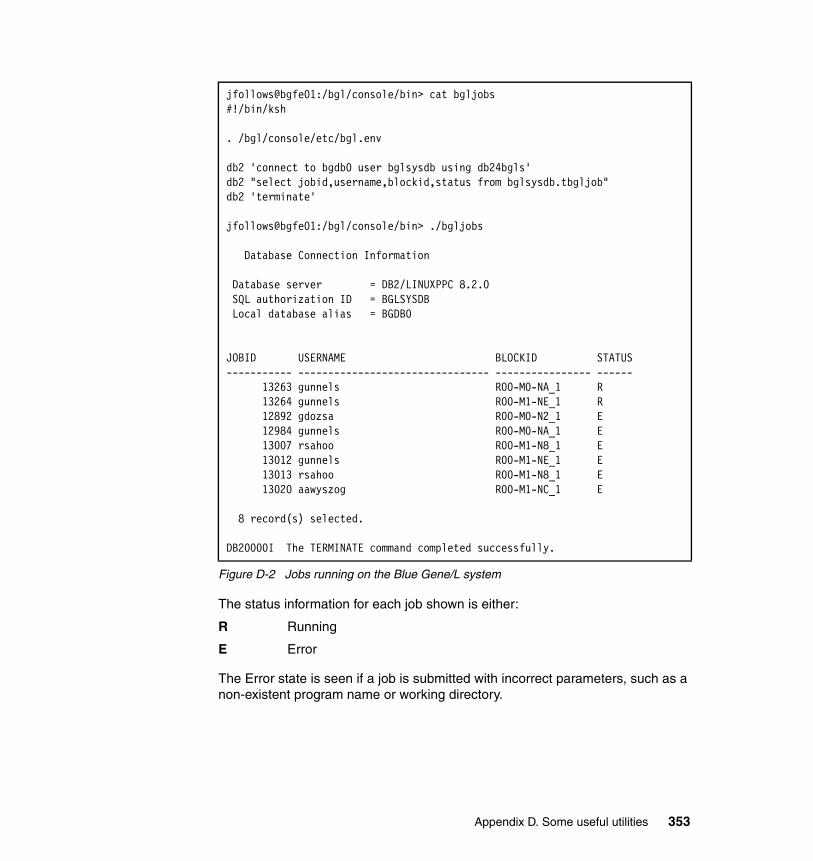
Figure D-2 Jobs running on the Blue Gene/L system

The status information for each job shown is either:

R Running

E Error

The Error state is seen if a job is submitted with incorrect parameters, such as a non-existent program name or working directory.

jfollows@bgfe01:/bgl/console/bin> cat bgljobs#!/bin/ksh


db2 'connect to bgdb0 user bglsysdb using db24bgls'db2 "select jobid,username,blockid,status from bglsysdb.tbgljob"db2 'terminate'

jfollows@bgfe01:/bgl/console/bin> ./bgljobs



JOBID USERNAME BLOCKID STATUS----------- -------------------------------- ---------------- ------ 13263 gunnels R00-M0-NA_1 R 13264 gunnels R00-M1-NE_1 R 12892 gdozsa R00-M0-N2_1 E 12984 gunnels R00-M0-NA_1 E 13007 rsahoo R00-M1-N8_1 E 13012 gunnels R00-M1-NE_1 E 13013 rsahoo R00-M1-N8_1 E 13020 aawyszog R00-M1-NC_1 E



Appendix D. Some useful utilities 353

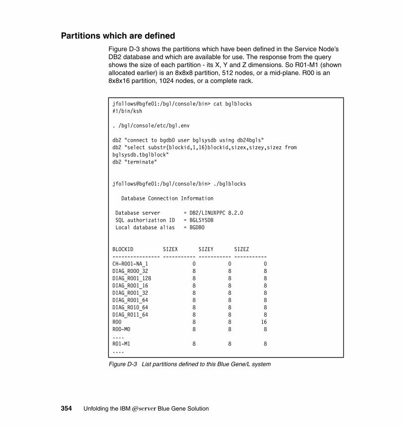
Partitions which are definedFigure D-3 shows the partitions which have been defined in the Service Node’s DB2 database and which are available for use. The response from the query shows the size of each partition - its X, Y and Z dimensions. So R01-M1 (shown allocated earlier) is an 8x8x8 partition, 512 nodes, or a mid-plane. R00 is an 8x8x16 partition, 1024 nodes, or a complete rack.

Figure D-3 List partitions defined to this Blue Gene/L system

jfollows@bgfe01:/bgl/console/bin> cat bglblocks#!/bin/ksh


db2 "connect to bgdb0 user bglsysdb using db24bgls"db2 "select substr(blockid,1,16)blockid,sizex,sizey,sizez from bglsysdb.tbglblock"db2 "terminate"

jfollows@bgfe01:/bgl/console/bin> ./bglblocks



BLOCKID SIZEX SIZEY SIZEZ ---------------- ----------- ----------- -----------CH-R001-NA_1 0 0 0DIAG_R000_32 8 8 8DIAG_R001_128 8 8 8DIAG_R001_16 8 8 8DIAG_R001_32 8 8 8DIAG_R001_64 8 8 8DIAG_R010_64 8 8 8DIAG_R011_64 8 8 8R00 8 8 16R00-M0 8 8 8....R01-M1 8 8 8....


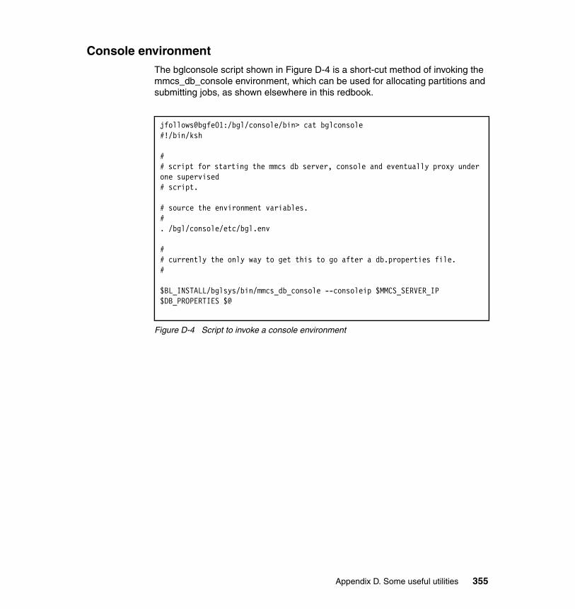
Console environmentThe bglconsole script shown in Figure D-4 is a short-cut method of invoking the mmcs_db_console environment, which can be used for allocating partitions and submitting jobs, as shown elsewhere in this redbook.

Figure D-4 Script to invoke a console environment

jfollows@bgfe01:/bgl/console/bin> cat bglconsole#!/bin/ksh

## script for starting the mmcs db server, console and eventually proxy under one supervised# script.

# source the environment variables.#. /bgl/console/etc/bgl.env

## currently the only way to get this to go after a db.properties file.#

$BL_INSTALL/bglsys/bin/mmcs_db_console --consoleip $MMCS_SERVER_IP $DB_PROPERTIES $@

Appendix D. Some useful utilities 355


Appendix E. Compiler configuration file

Because all compilation for Blue Gene/L is performed on the front end nodes, it is a cross-compilation process.

The default compiler installation allows compilation to take place with the target execution environment the same as the compilation environment.

As one example, the C compiler is invoked using the command blrts_xlc in place of the normal command xlc, which invokes the C compiler with an alternative compiler options file. The script which invokes the C compiler for Blue Gene/L is shown in Figure E-1.

E


Figure E-1 Customised compiler invocation command script

Other scripts are provided for different C and FORTRAN compiler invocations.

Sample compiler options fileExample E-1 shows the complete compiler options file used for Blue Gene/L, /etc/opt/ibmcmp/blrts.cfg. This options file is used in place of the default compiler options file by using the compiler invocation commands such as blrts_xlc in place of the normal xlc. This single compiler options file is used for all cross-compilation environment for Blue Gene/L, including FORTRAN as well as C.

Example: E-1 Compiler default options for cross-compilation for Blue Gene/L

* Configuration file generated on "Thu Dec 9 12:49:46 CST 2004"* with "/opt/ibmcmp/vac/7.0/bin/vac_configure -smprt /opt/ibmcmp/xlsmp/1.5 -mass /opt/ibmcmp/xlmass/4.1 -vac /opt/ibmcmp/vac/7.0 -install /opt/ibmcmp/vac/7.0/etc/vac.base.cfg -gcc /usr -gcc64 /usr -vacpp /opt/ibmcmp/vacpp/7.0 -vacpprt /opt/ibmcmp/vacpp/7.0 -vaclic /opt/ibmcmp/vac/7.0"* GCC version used: "3.3.3"* Configuration file generated on "Thu Dec 9 12:50:34 CST 2004"* with "/opt/ibmcmp/xlf/9.1/bin/xlf_configure -smprt /opt/ibmcmp/xlsmp/1.5 -mass /opt/ibmcmp/xlmass/4.1 -xlf /opt/ibmcmp/xlf/9.1 -install /opt/ibmcmp/xlf/9.1/etc/xlf.base.cfg -gcc /usr -gcc64 /usr -xlfrt /opt/ibmcmp/xlf/9.1 -xlflic /opt/ibmcmp/xlf/9.1"* GCC version used: "3.3.3"** Licensed Materials - Property of IBM* IBM XL C/C++ Enterprise Edition V7.0* 5724-I11* IBM(R) XL Fortran Advanced Edition V9.1 for Linux(R)* 5724-K76

jfollows@bgfe01:/opt/ibmcmp/vac/7.0/bin> cat blrts_xlc#!/bin/bash

export XL_CONFIG=ècho ${0} | sed -e 's#/opt/ibmcmp/.*$#/etc/opt/ibmcmp/#'``basename ${0%_*}`.cfgblrtscmd="`dirname ${0%_*}`/${0##*_} $@"

if [ -n "$BLRTSDEBUG" ]; then echo "export XL_CONFIG=${XL_CONFIG}" echo "$blrtscmd"fiexec $blrtscmd


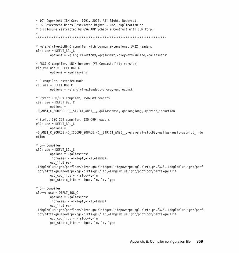
* (C) Copyright IBM Corp. 1991, 2004. All Rights Reserved.* US Government Users Restricted Rights - Use, duplication or* disclosure restricted by GSA ADP Schedule Contract with IBM Corp.***************************************************************************

* -qlanglvl=extc89 C compiler with common extensions, UNIX headersxlc: use = DEFLT_BGL_C options = -qlanglvl=extc89,-qcpluscmt,-qkeyword=inline,-qalias=ansi

* ANSI C compiler, UNIX headers (V6 Compatibility version)xlc_v6: use = DEFLT_BGL_C options = -qalias=ansi

* C compiler, extended modecc: use = DEFLT_BGL_C options = -qlanglvl=extended,-qnoro,-qnoroconst

* Strict ISO/C89 compiler, ISO/C89 headersc89: use = DEFLT_BGL_C options = -D_ANSI_C_SOURCE,-D__STRICT_ANSI__,-qalias=ansi,-qnolonglong,-qstrict_induction

* Strict ISO C99 compiler, ISO C99 headersc99: use = DEFLT_BGL_C options = -D_ANSI_C_SOURCE,-D_ISOC99_SOURCE,-D__STRICT_ANSI__,-qlanglvl=stdc99,-qalias=ansi,-qstrict_induction

* C++ compilerxlC: use = DEFLT_BGL_C options = -qalias=ansi libraries = -lxlopt,-lxl,-libmc++ gcc_libdirs= -L/bgl/BlueLight/ppcfloor/blrts-gnu/lib/gcc-lib/powerpc-bgl-blrts-gnu/3.2,-L/bgl/BlueLight/ppcfloor/blrts-gnu/powerpc-bgl-blrts-gnu/lib,-L/bgl/BlueLight/ppcfloor/blrts-gnu/lib gcc_cpp_libs = -lstdc++,-lm gcc_static_libs = -lgcc,-lm,-lc,-lgcc

* C++ compilerxlc++: use = DEFLT_BGL_C options = -qalias=ansi libraries = -lxlopt,-lxl,-libmc++ gcc_libdirs= -L/bgl/BlueLight/ppcfloor/blrts-gnu/lib/gcc-lib/powerpc-bgl-blrts-gnu/3.2,-L/bgl/BlueLight/ppcfloor/blrts-gnu/powerpc-bgl-blrts-gnu/lib,-L/bgl/BlueLight/ppcfloor/blrts-gnu/lib gcc_cpp_libs = -lstdc++,-lm gcc_static_libs = -lgcc,-lm,-lc,-lgcc

Appendix E. Compiler configuration file 359

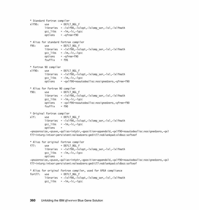
* Standard Fortran compilerxlf95: use = DEFLT_BGL_F libraries = -lxlf90,-lxlopt,-lxlomp_ser,-lxl,-lxlfmath gcc_libs = -lm,-lc,-lgcc options = -qfree=f90

* Alias for standard Fortran compilerf95: use = DEFLT_BGL_F libraries = -lxlf90,-lxlopt,-lxlomp_ser,-lxl,-lxlfmath gcc_libs = -lm,-lc,-lgcc options = -qfree=f90 fsuffix = f95

* Fortran 90 compilerxlf90: use = DEFLT_BGL_F libraries = -lxlf90,-lxlopt,-lxlomp_ser,-lxl,-lxlfmath gcc_libs = -lm,-lc,-lgcc options = -qxlf90=noautodealloc:nosignedzero,-qfree=f90

* Alias for Fortran 90 compilerf90: use = DEFLT_BGL_F libraries = -lxlf90,-lxlopt,-lxlomp_ser,-lxl,-lxlfmath gcc_libs = -lm,-lc,-lgcc options = -qxlf90=noautodealloc:nosignedzero,-qfree=f90 fsuffix = f90

* Original Fortran compilerxlf: use = DEFLT_BGL_F libraries = -lxlf90,-lxlopt,-lxlomp_ser,-lxl,-lxlfmath gcc_libs = -lm,-lc,-lgcc options = -qnozerosize,-qsave,-qalias=intptr,-qposition=appendold,-qxlf90=noautodealloc:nosignedzero,-qxlf77=intarg:intxor:persistent:noleadzero:gedit77:noblankpad:oldboz:softeof

* Alias for original Fortran compilerf77: use = DEFLT_BGL_F libraries = -lxlf90,-lxlopt,-lxlomp_ser,-lxl,-lxlfmath gcc_libs = -lm,-lc,-lgcc options = -qnozerosize,-qsave,-qalias=intptr,-qposition=appendold,-qxlf90=noautodealloc:nosignedzero,-qxlf77=intarg:intxor:persistent:noleadzero:gedit77:noblankpad:oldboz:softeof

* Alias for original Fortran compiler, used for XPG4 compliancefort77: use = DEFLT_BGL_F libraries = -lxlf90,-lxlopt,-lxlomp_ser,-lxl,-lxlfmath gcc_libs = -lm,-lc,-lgcc


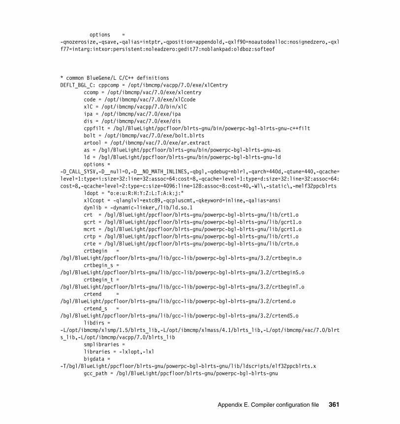
options = -qnozerosize,-qsave,-qalias=intptr,-qposition=appendold,-qxlf90=noautodealloc:nosignedzero,-qxlf77=intarg:intxor:persistent:noleadzero:gedit77:noblankpad:oldboz:softeof

* common BlueGene/L C/C++ definitionsDEFLT_BGL_C: cppcomp = /opt/ibmcmp/vacpp/7.0/exe/xlCentry ccomp = /opt/ibmcmp/vac/7.0/exe/xlcentry code = /opt/ibmcmp/vac/7.0/exe/xlCcode xlC = /opt/ibmcmp/vacpp/7.0/bin/xlC ipa = /opt/ibmcmp/vac/7.0/exe/ipa dis = /opt/ibmcmp/vac/7.0/exe/dis cppfilt = /bgl/BlueLight/ppcfloor/blrts-gnu/bin/powerpc-bgl-blrts-gnu-c++filt bolt = /opt/ibmcmp/vac/7.0/exe/bolt.blrts artool = /opt/ibmcmp/vac/7.0/exe/ar.extract as = /bgl/BlueLight/ppcfloor/blrts-gnu/bin/powerpc-bgl-blrts-gnu-as ld = /bgl/BlueLight/ppcfloor/blrts-gnu/bin/powerpc-bgl-blrts-gnu-ld options = -D_CALL_SYSV,-D__null=0,-D__NO_MATH_INLINES,-qbgl,-qdebug=nblrl,-qarch=440d,-qtune=440,-qcache=level=1:type=i:size=32:line=32:assoc=64:cost=8,-qcache=level=1:type=d:size=32:line=32:assoc=64:cost=8,-qcache=level=2:type=c:size=4096:line=128:assoc=8:cost=40,-Wl\,-static\,-melf32ppcblrts ldopt = "o:e:u:R:H:Y:Z:L:T:A:k:j:" xlCcopt = -qlanglvl=extc89,-qcpluscmt,-qkeyword=inline,-qalias=ansi dynlib = -dynamic-linker,/lib/ld.so.1 crt = /bgl/BlueLight/ppcfloor/blrts-gnu/powerpc-bgl-blrts-gnu/lib/crt1.o gcrt = /bgl/BlueLight/ppcfloor/blrts-gnu/powerpc-bgl-blrts-gnu/lib/gcrt1.o mcrt = /bgl/BlueLight/ppcfloor/blrts-gnu/powerpc-bgl-blrts-gnu/lib/gcrt1.o crtp = /bgl/BlueLight/ppcfloor/blrts-gnu/powerpc-bgl-blrts-gnu/lib/crti.o crte = /bgl/BlueLight/ppcfloor/blrts-gnu/powerpc-bgl-blrts-gnu/lib/crtn.o crtbegin = /bgl/BlueLight/ppcfloor/blrts-gnu/lib/gcc-lib/powerpc-bgl-blrts-gnu/3.2/crtbegin.o crtbegin_s = /bgl/BlueLight/ppcfloor/blrts-gnu/lib/gcc-lib/powerpc-bgl-blrts-gnu/3.2/crtbeginS.o crtbegin_t = /bgl/BlueLight/ppcfloor/blrts-gnu/lib/gcc-lib/powerpc-bgl-blrts-gnu/3.2/crtbeginT.o crtend = /bgl/BlueLight/ppcfloor/blrts-gnu/lib/gcc-lib/powerpc-bgl-blrts-gnu/3.2/crtend.o crtend_s = /bgl/BlueLight/ppcfloor/blrts-gnu/lib/gcc-lib/powerpc-bgl-blrts-gnu/3.2/crtendS.o libdirs = -L/opt/ibmcmp/xlsmp/1.5/blrts_lib,-L/opt/ibmcmp/xlmass/4.1/blrts_lib,-L/opt/ibmcmp/vac/7.0/blrts_lib,-L/opt/ibmcmp/vacpp/7.0/blrts_lib smplibraries = libraries = -lxlopt,-lxl bigdata = -T/bgl/BlueLight/ppcfloor/blrts-gnu/powerpc-bgl-blrts-gnu/lib/ldscripts/elf32ppcblrts.x gcc_path = /bgl/BlueLight/ppcfloor/blrts-gnu/powerpc-bgl-blrts-gnu


gcc_libdirs = -L/bgl/BlueLight/ppcfloor/blrts-gnu/lib/gcc-lib/powerpc-bgl-blrts-gnu/3.2,-L/bgl/BlueLight/ppcfloor/blrts-gnu/powerpc-bgl-blrts-gnu/lib,-L/bgl/BlueLight/ppcfloor/blrts-gnu/lib gcc_static_libs = -lgcc,-lm,-lc,-lgcc __GNUC_MINOR__ = 2 __GNUC_PATCHLEVEL__ = 0 __GNUC__ = 3 clm_path = /opt/clm_ibm crt2 = NULL defaultmsg = /opt/ibmcmp/vacpp/7.0/msg/en_US gcc_c_stdinc = /bgl/BlueLight/ppcfloor/blrts-gnu/lib/gcc-lib/powerpc-bgl-blrts-gnu/3.2/include:/bgl/BlueLight/ppcfloor/blrts-gnu/powerpc-bgl-blrts-gnu/sys-include gcc_cpp_stdinc = /bgl/BlueLight/ppcfloor/blrts-gnu/include/c++/3.2:/bgl/BlueLight/ppcfloor/blrts-gnu/include/c++/3.2/powerpc-bgl-blrts-gnu:/bgl/BlueLight/ppcfloor/blrts-gnu/include/c++/3.2/backward:/bgl/BlueLight/ppcfloor/blrts-gnu/lib/gcc-lib/powerpc-bgl-blrts-gnu/3.2/include:/bgl/BlueLight/ppcfloor/blrts-gnu/powerpc-bgl-blrts-gnu/sys-include modes_configure = 32_64 os_major = 9 os_minor = 0 os_patchlevel = 0 os_variant = bgl vac_path = /opt/ibmcmp/vac/7.0 vacpp_path = /opt/ibmcmp/vacpp/7.0 xlc_c_complexgccinc = /opt/ibmcmp/xlsmp/1.5/include:/opt/ibmcmp/xlmass/4.1/include:/opt/ibmcmp/vac/7.0/include:/bgl/BlueLight/ppcfloor/blrts-gnu/lib/gcc-lib/powerpc-bgl-blrts-gnu/3.2/include:/bgl/BlueLight/ppcfloor/blrts-gnu/powerpc-bgl-blrts-gnu/sys-include xlc_c_stdinc = /opt/ibmcmp/xlsmp/1.5/include:/opt/ibmcmp/xlmass/4.1/include:/opt/ibmcmp/vac/7.0/include xlc_cpp_complexgccinc = /opt/ibmcmp/xlsmp/1.5/include:/opt/ibmcmp/xlmass/4.1/include:/opt/ibmcmp/vacpp/7.0/include:/bgl/BlueLight/ppcfloor/blrts-gnu/include/c++/3.2:/bgl/BlueLight/ppcfloor/blrts-gnu/include/c++/3.2/powerpc-bgl-blrts-gnu:/bgl/BlueLight/ppcfloor/blrts-gnu/include/c++/3.2/backward:/bgl/BlueLight/ppcfloor/blrts-gnu/lib/gcc-lib/powerpc-bgl-blrts-gnu/3.2/include:/bgl/BlueLight/ppcfloor/blrts-gnu/powerpc-bgl-blrts-gnu/sys-include xlc_cpp_stdinc = /opt/ibmcmp/xlsmp/1.5/include:/opt/ibmcmp/xlmass/4.1/include:/opt/ibmcmp/vacpp/7.0/include xlcmp_path = /opt/ibmcmp/vac/7.0

* Common BlueGene/L Fortran definitionsDEFLT_BGL_F: xlf = /opt/ibmcmp/xlf/9.1/exe/xlfentry crt = /bgl/BlueLight/ppcfloor/blrts-gnu/powerpc-bgl-blrts-gnu/lib/crt1.o crtp = /bgl/BlueLight/ppcfloor/blrts-gnu/powerpc-bgl-blrts-gnu/lib/crti.o crte = /bgl/BlueLight/ppcfloor/blrts-gnu/powerpc-bgl-blrts-gnu/lib/crtn.o crtbegin = /bgl/BlueLight/ppcfloor/blrts-gnu/lib/gcc-lib/powerpc-bgl-blrts-gnu/3.2/crtbegin.o


crtend = /bgl/BlueLight/ppcfloor/blrts-gnu/lib/gcc-lib/powerpc-bgl-blrts-gnu/3.2/crtend.o crtsavres = /bgl/BlueLight/ppcfloor/blrts-gnu/lib/gcc-lib/powerpc-bgl-blrts-gnu/3.2/crtsavres.o mcrt = /bgl/BlueLight/ppcfloor/blrts-gnu/powerpc-bgl-blrts-gnu/lib/gcrt1.o gcrt = /bgl/BlueLight/ppcfloor/blrts-gnu/powerpc-bgl-blrts-gnu/lib/gcrt1.o include_32 = -I/opt/ibmcmp/xlf/9.1/include dis = /opt/ibmcmp/xlf/9.1/exe/dis code = /opt/ibmcmp/xlf/9.1/exe/xlfcode hot = /opt/ibmcmp/xlf/9.1/exe/xlfhot ipa = /opt/ibmcmp/xlf/9.1/exe/ipa bolt = /opt/ibmcmp/xlf/9.1/exe/bolt.blrts artool = /opt/ibmcmp/vac/9.1/exe/ar.extract defaultmsg = /opt/ibmcmp/xlf/9.1/msg/en_US as = /bgl/BlueLight/ppcfloor/blrts-gnu/bin/powerpc-bgl-blrts-gnu-as ld = /bgl/BlueLight/ppcfloor/blrts-gnu/bin/powerpc-bgl-blrts-gnu-ld cppoptions = -C cpp = /opt/ibmcmp/xlf/9.1/exe/cpp dynlib = -dynamic-linker,/lib/ld.so.1 libdirs = -L/opt/ibmcmp/xlsmp/1.5/blrts_lib,-L/opt/ibmcmp/xlmass/4.1/blrts_lib,-L/opt/ibmcmp/xlf/9.1/blrts_lib gcc_path = /bgl/BlueLight/ppcfloor/blrts-gnu/powerpc-bgl-blrts-gnu gcc_libdirs= -L/bgl/BlueLight/ppcfloor/blrts-gnu/lib/gcc-lib/powerpc-bgl-blrts-gnu/3.2,-L/bgl/BlueLight/ppcfloor/blrts-gnu/powerpc-bgl-blrts-gnu/lib,-L/bgl/BlueLight/ppcfloor/blrts-gnu/lib bigdata = -T/bgl/BlueLight/ppcfloor/blrts-gnu/powerpc-bgl-blrts-gnu/lib/ldscripts/elf32ppcblrts.x options = -qbgl,-qdebug=nblrl,-qarch=440d,-qtune=440,-qcache=level=1:type=i:size=32:line=32:assoc=64:cost=8,-qcache=level=1:type=d:size=32:line=32:assoc=64:cost=8,-qcache=level=2:type=c:size=4096:line=128:assoc=8:cost=40,-Wl\,-static\,-melf32ppcblrts __GNUC_MINOR__ = 2 __GNUC_PATCHLEVEL__ = 0 __GNUC__ = 3 clm_path = /opt/clm_ibm crt2 = NULL modes_configure = 32_64 os_major = 9 os_minor = 0 os_patchlevel = 0 os_variant = bgl xlcmp_path = /opt/ibmcmp/xlf/9.1 xlf_path = /opt/ibmcmp/xlf/9.1



Appendix F. Systems comparison

Blue Gene/L and other contemporary architecturesWe use the following three areas to compare Blue Gene/L with some of the commercially successful distributed systems:

� Node or system

� Communication network

� Operating system

Our comparison, based on this classification, is helpful in assessing the relative merits of these potentially competing archtiectures and in discussing the characterization of application sets for which Blue Gene/L can be a suitable hardware platform.

First, we look at the information in the following three tables about Blue Gene/L and current commercial computing systems. The tables give a nutshell view of Blue Gene/L, which facilitates meaningful comparison. A more detailed treatment of these features is provided in later chapters of this publication.

Table F-1 lists information about the nodes used in Blue Gene/L and other hardware platforms and their operational characteristics. Fill in the remaining data when you perform your own comparison.

F


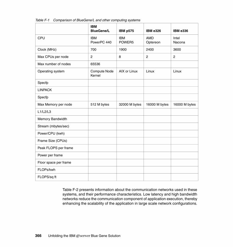
Table F-1 Comparison of BlueGene/L and other computing systems

Table F-2 presents information about the communication networks used in these systems, and their performance characteristics. Low latency and high bandwidth networks reduce the communication component of application execution, thereby enhancing the scalability of the application in large scale network configurations.

IBM BlueGene/L IBM p575 IBM e326 IBM e336

CPU IBM PowerPC 440

IBMPOWER5

AMD Optereon

Intel Nacona

Clock (MHz) 700 1900 2400 3600

Max CPUs per node 2 8 2 2

Max number of nodes 65536

Operating system Compute Node Kernel

AIX or Linux Linux Linux

Specfp

LINPACK

Specfp

Max Memory per node 512 M bytes 32000 M bytes 16000 M bytes 16000 M bytes

L1/L2/L3

Memory Bandwidth

Stream (mbytes/sec)

Power/CPU (kwh)

Frame Size (CPUs)

Peak FLOPS per frame

Power per frame

Floor space per frame

FLOPs/kwh

FLOPS/sq ft


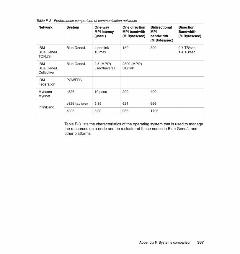
Table F-2 Performance comparison of communicaiton networks

Table F-3 lists the characteristics of the operating system that is used to manage the resources on a node and on a cluster of these nodes in Blue Gene/L and other platforms.

Network System One-way MPI latency(µsec )

One directionMPI bandwith(M Bytes/sec)

BidirectionalMPI bandwidth(M Bytes/sec)

BisectionBandwidth(M Bytes/sec)

IBM Blue Gene/L TORUS

Blue Gene/L 4 per link10 max

150 300 0.7 TB/sec1.4 TB/sec

IBM Blue Gene/L Collective

Blue Gene/L 2.5 (MPI?)µsec/traversal

2800 (MPI?)GB/link

IBM Federation

POWER5

MyricomMyrinet

e326 10 µsec 200 400

InfiniBande326 (2.2 GHz) 5.35 621 666

e336 5.03 965 1725

Appendix F. Systems comparison 367

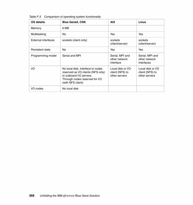
Table F-3 Comparison of operating system functionality

OS details Blue Gene/L CNK AIX Linux

Memory 6 MB

Multitasking No Yes Yes

External interfaces sockets (client only) sockets (client/server)

sockets (client/server)

Persistent state No Yes Yes

Programming model Serial and MPI Serial, MPI and other network interface

Serial, MPI and other network interfaces

I/O No local disk, interface to nodes reserved as I/O clients (NFS only) to outboard I/O servers.Through nodes reserved for I/O (with NFS client)

Local disk or I/O client (NFS) to other servers

Local disk or I/O client (NFS) to other servers

I/O nodes No local disk


Appendix G. Hardware counters

On Blue Gene/L, the bgl_perfctr interface is a user-level API that provides access to the universal performance counter unit (UPC) and double floating point unit (FPU) counters. The bgl_perfctr interface presents the user with a set of 52 virtual 64-bit counters that map to the underlying hardware counters. The first 48 counters map to the UPC counters on the chip, while the last four counters map to the two counters in each of the double FPUs, one counter for arithmetic operations and one counter for load and store operations.

The user instantiates counters by requesting to register a certain event. All possible events are available as mnemonics. Given a request to register an event, the library interface locates an available hardware counter capable of registering the particular event. It this search is successful the event is registered as an event pending to be added. If there is no available hardware counter for the event, an error code is returned to the user.

The counters pending to be added get invoked through the user initiating a call to bgl_perfctr_commit(). At this point all pending changes to the counter setup is performed and the counter map is updated. A call to bgl_perfctr_revoke() will clear all pending changes and leave the hardware counters untouched.

The virtual counters in the bgl_perfctr interface are updated from the actual hardware counters by calling bgl_perfctr_update() directly. Also, calling any of the functions bgl_perfctr_copy_counters(), bgl_perfctr_copy_state() or bgl_perfctr_get_counters() will implicitly call bgl_perfctr_update(). The virtual counter update reads all active hardware counters and updates the

G


corresponding virtual counter with the number of counts aggregated since the latest read. The configured UPC counters are read through the memory map interface, while FPU counters are read through DCR access.

At library initialization, which is explicitly made by the user, the user can set up the library to periodically call bgl_perfctr_update() by means of a periodic timer interrupt. This interrupt will occur with an interval of approximately 6s (on a 700MHz system), which will guard against any 32-bit counter overflowing more than once between updates to the virtual counters. By default this interval timer will be set up after synchronization between all nodes in the partition. This will reduce the impact on a parallel running application from the periodic virtual counter updates.

G.1 Link with bgl_perfctr library on Blue Gene/LThe bgl_perfctr library libbgl_perfctr.rts.a is located in:

/bgl/BlueLight/ppcfloor/bglsys/lib

The header file for the C/C++ language is located in:

/bgl/BlueLight/ppcfloor/bglsys/include/bgl_perfctr.h

G.2 API detailsA list of the first 100 defined event mnemonics is provided in Figure G-1 on page 371, to illustrate the naming scheme. The complete list is provided in:

/bgl/BlueLight/ppcfloor/bglsys/include/bgl_perfctr_events.h

These mnemonics define an enumerated data type that is used to identify the events in bgl_perfctr. A full event descriptor is a structure with two components: the event mnemonic, and the edge or state to monitor. The definition of the event descriptor is shown in Example 8-10 on page 371, together with an example of its use. UPC events need to specify both an event type and an edge type to be complete. For FPU events the edge selector is not used and should always be set to zero.

In Example 8-10, two examples of events are shown. The first event will count multiplies and divides in FPU0, while the second will count the duration in UPC cycles (CLOCKx2 cycles) where there were 3 outstanding read requests in CPU core 0. All durations are in the unit of UPC cycles, which is equal to two CPU cycles.


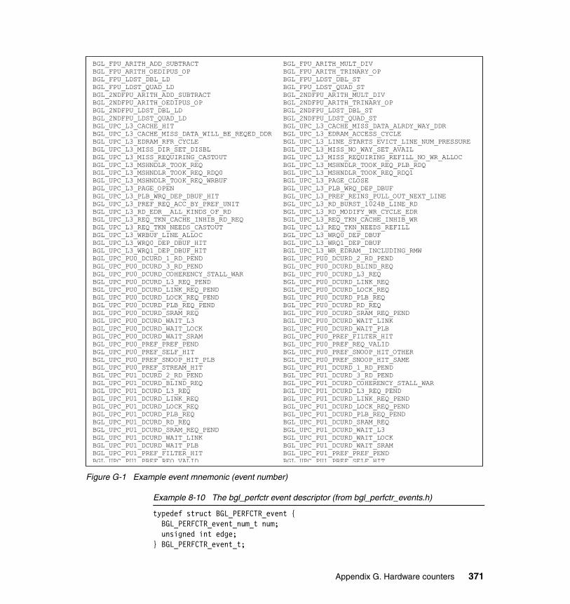
Figure G-1 Example event mnemonic (event number)

Example 8-10 The bgl_perfctr event descriptor (from bgl_perfctr_events.h)

typedef struct BGL_PERFCTR_event { BGL_PERFCTR_event_num_t num; unsigned int edge;} BGL_PERFCTR_event_t;

BGL_FPU_ARITH_ADD_SUBTRACT BGL_FPU_ARITH_MULT_DIV BGL_FPU_ARITH_OEDIPUS_OP BGL_FPU_ARITH_TRINARY_OP BGL_FPU_LDST_DBL_LD BGL_FPU_LDST_DBL_ST BGL_FPU_LDST_QUAD_LD BGL_FPU_LDST_QUAD_ST BGL_2NDFPU_ARITH_ADD_SUBTRACT BGL_2NDFPU_ARITH_MULT_DIV BGL_2NDFPU_ARITH_OEDIPUS_OP BGL_2NDFPU_ARITH_TRINARY_OP BGL_2NDFPU_LDST_DBL_LD BGL_2NDFPU_LDST_DBL_ST BGL_2NDFPU_LDST_QUAD_LD BGL_2NDFPU_LDST_QUAD_ST BGL_UPC_L3_CACHE_HIT BGL_UPC_L3_CACHE_MISS_DATA_ALRDY_WAY_DDR BGL_UPC_L3_CACHE_MISS_DATA_WILL_BE_REQED_DDR BGL_UPC_L3_EDRAM_ACCESS_CYCLE BGL_UPC_L3_EDRAM_RFR_CYCLE BGL_UPC_L3_LINE_STARTS_EVICT_LINE_NUM_PRESSURE BGL_UPC_L3_MISS_DIR_SET_DISBL BGL_UPC_L3_MISS_NO_WAY_SET_AVAIL BGL_UPC_L3_MISS_REQUIRING_CASTOUT BGL_UPC_L3_MISS_REQUIRING_REFILL_NO_WR_ALLOC BGL_UPC_L3_MSHNDLR_TOOK_REQ BGL_UPC_L3_MSHNDLR_TOOK_REQ_PLB_RDQ BGL_UPC_L3_MSHNDLR_TOOK_REQ_RDQ0 BGL_UPC_L3_MSHNDLR_TOOK_REQ_RDQ1 BGL_UPC_L3_MSHNDLR_TOOK_REQ_WRBUF BGL_UPC_L3_PAGE_CLOSE BGL_UPC_L3_PAGE_OPEN BGL_UPC_L3_PLB_WRQ_DEP_DBUF BGL_UPC_L3_PLB_WRQ_DEP_DBUF_HIT BGL_UPC_L3_PREF_REINS_PULL_OUT_NEXT_LINE BGL_UPC_L3_PREF_REQ_ACC_BY_PREF_UNIT BGL_UPC_L3_RD_BURST_1024B_LINE_RD BGL_UPC_L3_RD_EDR__ALL_KINDS_OF_RD BGL_UPC_L3_RD_MODIFY_WR_CYCLE_EDR BGL_UPC_L3_REQ_TKN_CACHE_INHIB_RD_REQ BGL_UPC_L3_REQ_TKN_CACHE_INHIB_WR BGL_UPC_L3_REQ_TKN_NEEDS_CASTOUT BGL_UPC_L3_REQ_TKN_NEEDS_REFILL BGL_UPC_L3_WRBUF_LINE_ALLOC BGL_UPC_L3_WRQ0_DEP_DBUF BGL_UPC_L3_WRQ0_DEP_DBUF_HIT BGL_UPC_L3_WRQ1_DEP_DBUF BGL_UPC_L3_WRQ1_DEP_DBUF_HIT BGL_UPC_L3_WR_EDRAM__INCLUDING_RMW BGL_UPC_PU0_DCURD_1_RD_PEND BGL_UPC_PU0_DCURD_2_RD_PEND BGL_UPC_PU0_DCURD_3_RD_PEND BGL_UPC_PU0_DCURD_BLIND_REQ BGL_UPC_PU0_DCURD_COHERENCY_STALL_WAR BGL_UPC_PU0_DCURD_L3_REQ BGL_UPC_PU0_DCURD_L3_REQ_PEND BGL_UPC_PU0_DCURD_LINK_REQ BGL_UPC_PU0_DCURD_LINK_REQ_PEND BGL_UPC_PU0_DCURD_LOCK_REQ BGL_UPC_PU0_DCURD_LOCK_REQ_PEND BGL_UPC_PU0_DCURD_PLB_REQ BGL_UPC_PU0_DCURD_PLB_REQ_PEND BGL_UPC_PU0_DCURD_RD_REQ BGL_UPC_PU0_DCURD_SRAM_REQ BGL_UPC_PU0_DCURD_SRAM_REQ_PEND BGL_UPC_PU0_DCURD_WAIT_L3 BGL_UPC_PU0_DCURD_WAIT_LINK BGL_UPC_PU0_DCURD_WAIT_LOCK BGL_UPC_PU0_DCURD_WAIT_PLB BGL_UPC_PU0_DCURD_WAIT_SRAM BGL_UPC_PU0_PREF_FILTER_HIT BGL_UPC_PU0_PREF_PREF_PEND BGL_UPC_PU0_PREF_REQ_VALID BGL_UPC_PU0_PREF_SELF_HIT BGL_UPC_PU0_PREF_SNOOP_HIT_OTHER BGL_UPC_PU0_PREF_SNOOP_HIT_PLB BGL_UPC_PU0_PREF_SNOOP_HIT_SAME BGL_UPC_PU0_PREF_STREAM_HIT BGL_UPC_PU1_DCURD_1_RD_PEND BGL_UPC_PU1_DCURD_2_RD_PEND BGL_UPC_PU1_DCURD_3_RD_PEND BGL_UPC_PU1_DCURD_BLIND_REQ BGL_UPC_PU1_DCURD_COHERENCY_STALL_WAR BGL_UPC_PU1_DCURD_L3_REQ BGL_UPC_PU1_DCURD_L3_REQ_PEND BGL_UPC_PU1_DCURD_LINK_REQ BGL_UPC_PU1_DCURD_LINK_REQ_PEND BGL_UPC_PU1_DCURD_LOCK_REQ BGL_UPC_PU1_DCURD_LOCK_REQ_PEND BGL_UPC_PU1_DCURD_PLB_REQ BGL_UPC_PU1_DCURD_PLB_REQ_PEND BGL_UPC_PU1_DCURD_RD_REQ BGL_UPC_PU1_DCURD_SRAM_REQ BGL_UPC_PU1_DCURD_SRAM_REQ_PEND BGL_UPC_PU1_DCURD_WAIT_L3 BGL_UPC_PU1_DCURD_WAIT_LINK BGL_UPC_PU1_DCURD_WAIT_LOCK BGL_UPC_PU1_DCURD_WAIT_PLB BGL_UPC_PU1_DCURD_WAIT_SRAM BGL_UPC_PU1_PREF_FILTER_HIT BGL_UPC_PU1_PREF_PREF_PEND BGL UPC PU1 PREF REQ VALID BGL UPC PU1 PREF SELF HIT

Appendix G. Hardware counters 371

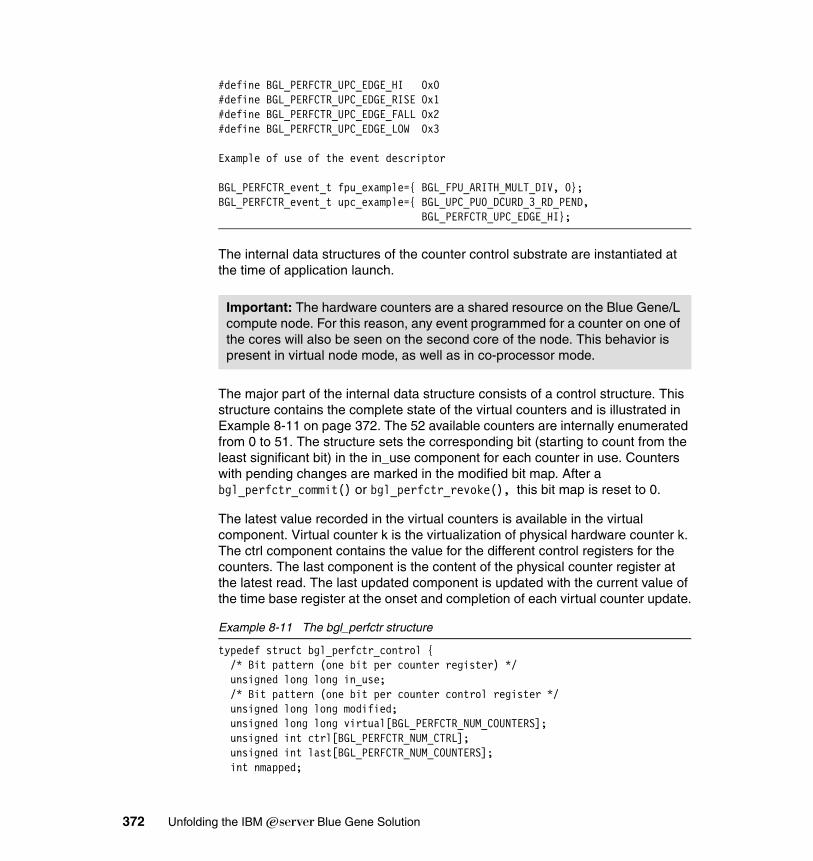
#define BGL_PERFCTR_UPC_EDGE_HI 0x0#define BGL_PERFCTR_UPC_EDGE_RISE 0x1#define BGL_PERFCTR_UPC_EDGE_FALL 0x2#define BGL_PERFCTR_UPC_EDGE_LOW 0x3

Example of use of the event descriptor

BGL_PERFCTR_event_t fpu_example={ BGL_FPU_ARITH_MULT_DIV, 0};BGL_PERFCTR_event_t upc_example={ BGL_UPC_PU0_DCURD_3_RD_PEND, BGL_PERFCTR_UPC_EDGE_HI};

The internal data structures of the counter control substrate are instantiated at the time of application launch.

The major part of the internal data structure consists of a control structure. This structure contains the complete state of the virtual counters and is illustrated in Example 8-11 on page 372. The 52 available counters are internally enumerated from 0 to 51. The structure sets the corresponding bit (starting to count from the least significant bit) in the in_use component for each counter in use. Counters with pending changes are marked in the modified bit map. After a bgl_perfctr_commit() or bgl_perfctr_revoke(), this bit map is reset to 0.

The latest value recorded in the virtual counters is available in the virtual component. Virtual counter k is the virtualization of physical hardware counter k. The ctrl component contains the value for the different control registers for the counters. The last component is the content of the physical counter register at the latest read. The last updated component is updated with the current value of the time base register at the onset and completion of each virtual counter update.

Example 8-11 The bgl_perfctr structure

typedef struct bgl_perfctr_control { /* Bit pattern (one bit per counter register) */ unsigned long long in_use; /* Bit pattern (one bit per counter control register */ unsigned long long modified; unsigned long long virtual[BGL_PERFCTR_NUM_COUNTERS]; unsigned int ctrl[BGL_PERFCTR_NUM_CTRL]; unsigned int last[BGL_PERFCTR_NUM_COUNTERS]; int nmapped;

Important: The hardware counters are a shared resource on the Blue Gene/L compute node. For this reason, any event programmed for a counter on one of the cores will also be seen on the second core of the node. This behavior is present in virtual node mode, as well as in co-processor mode.


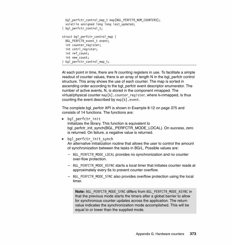
bgl_perfctr_control_map_t map[BGL_PERFCTR_NUM_COUNTERS]; volatile unsigned long long last_updated;} bgl_perfctr_control_t;

struct bgl_perfctr_control_map { BGL_PERFCTR_event_t event; int counter_register; int cntrl_register; int ref_count; int new_count;} bgl_perfctr_control_map_t;

At each point in time, there are N counting registers in use. To facilitate a simple readout of counter values, there is an array of length N in the bgl_perfctr control structure. This array shows the use of each counter. The map is sorted in ascending order according to the bgl_perfctr event descriptor enumerator. The number of active events, N, is stored in the component nmapped. The virtual/physical counter map[k].counter_register, where k<nmapped, is thus counting the event described by map[k].event.

The complete bgl_perfctr API is shown in Example 8-12 on page 375 and consists of 14 functions. The functions are:

� bgl_perfctr_init Initializes the library. This function is equivalent to bgl_perfctr_init_synch(BGL_PERFCTR_MODE_LOCAL). On success, zero is returned. On failure, a negative value is returned.

� bgl_perfctr_init_synch An alternative initialization routine that allows the user to control the amount of synchronization between the tasks in BG/L. Possible values are:

– BGL_PERFCTR_MODE_LOCAL provides no synchronization and no counter over-flow protection.

– BGL_PERFCTR_MODE_ASYNC starts a local timer that initiates counter reads at approximately every 6s to prevent counter overflow.

– BGL_PERFCTR_MODE_SYNC also provides overflow protection using the local timer.

Note: BGL_PERFCTR_MODE_SYNC differs from BGL_PERFCTR_MODE_ASYNC in that the previous mode starts the timers after a global barrier to allow for synchronous counter updates across the application. The return value indicates the synchronization mode accomplished. This will be equal to or lower than the supplied mode.


� bgl_perfctr_shutdownStops local timed interrupts on the local core, and if there is no core using the counters, clears the internal state and stops all counters.

� bgl_perfctr_add_eventAttempts to schedule an event to be added to the running set of counters.

� bgl_perfctr_remove_eventAttempts to schedule an event to be removed from the running set of counters.

� int bgl_perfctr_commitCommits all pending changes to the running set of counters.

� int bgl_perfctr_revokeRemoves all pending changes and restores the internal state of the library to the running set of counters.

� int bgl_perfctr_updateUpdates the virtual counters with the current value of the hardware counters.

� int bgl_perfctr_copy_countersUpdates the virtual counters with the current value of the counters, and provides a copy of the virtual counter values in the supplied buffer.

� int bgl_perfctr_copy_hwstateUpdates the virtual counters with the current value of the counters, and provides a copy of the complete internal state of the library in the supplied buffer. This dump includes the information of all configured counters, as well as the value of the virtual counters after the update.

� int bgl_perfctr_dump_stateDumps the complete state of the library to a provided file handle. This function is mainly intended for debugging code that uses the bgl_perfctr interface.

� bgl_perfctr_control_t* bgl_perfctr_hwstateGets a pointer to the internal state of the bgl_perfctr interface.

� int bgl_perfctr_get_countersTakes the lock on the internal virtual counters and updates the virtual counters with the current value of the hardware counters. The function returns without releasing the lock.

� int bgl_perfctr_release_countersReleases the lock taken by bgl_perfctr_get_counters().

The end user will typically not be interested in accessing the content of the control registers in the bgl_perfctr control structure, but the information is available. For asymmetric counters where read and write bit patterns are not the same, bgl_perfctr uses the write pattern. That is, any time bgl_perfctr reads a


counter control register state from the hardware, it is translated into its corresponding write bit-order in the library layer.

Example 8-12 The bgl_perfctr API (bgl_perfctr.h)

int bgl_perfctr_init(void);int bgl_perfctr_init_synch(int mode);int bgl_perfctr_shutdown();int bgl_perfctr_add_event(BGL_PERFCTR_event_t event);int bgl_perfctr_remove_event(BGL_PERFCTR_event_t event);int bgl_perfctr_commit();int bgl_perfctr_revoke();int bgl_perfctr_dump_state(FILE *fh);int bgl_perfctr_update();int bgl_perfctr_copy_counters(unsigned long long values[],

size_t size_of_values);int bgl_perfctr_copy_state(bgl_perfctr_control_t *hw_state,

size_t size_of_buffer);bgl_perfctr_control_t *bgl_perfctr_hwstate(void);inline unsigned long long *bgl_perfctr_get_counters(void);inline void bgl_perfctr_release_counters(void);

G.3 Ways of accessing the countersAs the counters are a shared resource, care must be taken when accessing the virtual counters. Under normal conditions, the use of the library interface is straightforward. When there are multiple agents involved in accessing the counter, substrate application code needs to take this into account; otherwise, results may appear confusing.

As the virtual counters may be updated by either of the cores and also can be updated by interval timer controlled interrupts, the value of the virtual counters may change between a user-induced counter update and a subsequent access to the memory location of the virtual counter. Depending on the degree of control users of the library need on this behavior, any of the following calling sequences can be used.

G.3.1 Counter update and copy-out A call to the function bgl_perfctr_copy_counters() updates the internal virtual counters and copies their updated values to the user-provided memory buffer. The update and copy is made within a lock of the virtual counters to guarantee coherence.


G.3.2 Counter update and immediate accessIn cases where the user knows that no other agent will be accessing the counters in between an initiated virtual counter update and a read-out of the counter values, or if such updates will have negligible influence on the results, the bgl_perfctr_update() function can be used. After the update, the user can read the current values of the virtual counters from the SRAM memory region. The memory address of the virtual counters are given by bgl_perfctr_hwstat()->virtual.

There should be only a short code path between the call to the update function and the read-out of the counters, since further updates to the counters may occur if user code on the other core executes the update function or if the timed update feature sets in. With a short code path, such updates will produce a low amount of update increments to the virtual counters.

G.3.3 Counter update and lockAdvanced users that want complete control of the behavior of the library between the counter update and counter read-out without taking the overhead of the bgl_pefctr_copy_counters() function can use the acquire and lock function provided in bgl_perfctr_get_counters(). This call will acquire a lock of the virtual counters and then update their content with the current value of the hardware counters.

While the lock is held, timed interrupt updates of the counters from any core is automatically disabled and access to the virtual counters from the other CPU core is blocked. Application code can read the content of the virtual counter content, as described in the previous section. It is essential that the lock of the virtual counters is released by the function bgl_perfctr_release_counters().

G.4 Available counter eventsBgl_perfctr provides a static array, BGL_PERFCTR_event_table[], shown in Example 8-13, with one entry per hardware event on the Blue Gene/L compute node. This table is indexed using a C enumerated type, the event number and can be used to find out all details about the event. For each event, the field num_encodings denotes in how many different locations of the hardware the event can be located. For each such location, the encoding[] field lists the counter group, the counter number within the group, and the actual code used to program the event in that location.

The event table also provides fields for the mnemonic name of the event and a description of the event, to facilitate event number to descriptive string


translations. This table need not be used by the user, but it provides easy and accurate access to information on possible counter allocations and event descriptions.

Example 8-13 The event information table BGL_PERFCTR_event_table

BGL_PERFCTR_event_encoding { unsigned int group; /* Which counter group to use */ unsigned int counter; /* Which counter {A,B,C} to use */ unsigned int code; /* Which hw-counter code */} BGL_PERFCTR_event_encoding_t;

typedef const struct BGL_PERFCTR_event_descr { BGL_PERFCTR_event_num_t event_num; int num_encodings; u_int64_t mapping; BGL_PERFCTR_event_encoding_t encoding[BGL_PERFCTR_MAX_ENCODINGS]; const char *event_name; const char *event_descr;} BGL_PERFCTR_event_descr_t;

BGL_PERFCTR_event_descr_t BGL_PERFCTR_event_table[BGL_PERFCTR_NUMEVENTS];

G.5 Correct API usageThe bgl_perfctr library and its API is an abstraction of the underlying hardware. As such, it shares some of the properties of the physical counters. This becomes important when used by advanced users in a multi-threaded fashion. Predictable behavior will be the result when the following recommendations are honored.

G.5.1 Using the second CPUCalls to the bgl_perfctr library can be made from either CPU on the compute node. The library does the necessary locking internally to guarantee coherency of the virtual counters with the hardware counters.

Calls that modify counter control register content can be used on either CPU core. bgl_perfctr_add_event(), bgl_perfctr_remove_event(), bgl_perfctr_revoke() work transparently by the internal use of the reference count in the library. Thus, if the same event is added by both cores, the reference count of that event will be 2. The event will start counting at the first time the bgl_perfctr_commit() function is called after the event has been added. The event will not disappear from the configured counters until the reference count


has dropped to 0 and a subsequent commit operation has been performed by any core.

Library initialization is either a local or a global operation, depending on the mode selected. Initializing the user level counters using the bgl_perfctr_init() function is equivalent to bgl_perfctr_init_synch with an argument of BGL_PERFCTR_MODE_LOCAL. In this mode as well as in the other modes, the virtual counter structure is a shared resource between the CPU cores on the compute node. In local mode it is the responsibility of the user to make sure that calls to bgl_perfctr_update() are performed frequently enough to ensure that the 32-bit hardware counters do not collect more than 232-1 events in between calls. bgl_perfctr_update() can be called directly, but it can also be called indirectly using the functions bgl_perfctr_copy_counters() and bgl_perfctr_copy_state().

Automatic prevention of counter overflow can be achieved by providing the argument BGL_PERFCTR_MODE_ASYNC or BGL_PERFCTR_MODE_SYNC to bgl_perfctr_init_synch(). In this mode, a user-level timed interrupt is installed that executes a virtual counter update within the passing of 232 CPU cycles.

The two modes differ in their global synchronization behavior. The synchronous mode executes a global barrier using the global barrier network together with local synchronization within the node using the CPU lockbox. The asynchronous mode does not perform this synchronization before starting the interval timer interrupts. A safety time-out of 5 seconds is used in the global barrier to safeguard for the cases when the global barrier is not available, for example, when not all nodes on a partition have user code loaded. The core synchronization on the local node is performed on all nodes that have two user applications loaded. This means, that virtual node mode can use the synchronous mode successfully in all cases where there are at least one process running on each node. Any nodes with two processes on them will take appropriate action to guarantee synchronization within the chip in parallel to the internode synchronization.

G.5.2 Counter start, stop, and resetIn bgl_perfctr there is no explicit start, stop, or reset of a counter. The underlying hardware counter will start incrementing at the moment the control word is written into the counter group control register. Start, stop, and reset of counters is accomplished by means of the update function (or functions) calls that have an update of the virtual counters as a side effect. This function call establishes a baseline for the virtual counters to which later returned values from the same function can be compared.


The PAPI library, which is implemented using bgl_perfctr, provides an API with full start, stop, and reset functionality.

G.5.3 Locking semantics of bgl_perfctrThe bgl_perfctr interface takes use of two locks internally to guarantee a coherent view of the counter state. One lock protects updates of the control data of the library, while the other lock is exclusively used to protect the virtual counters against incoherent updates. These two locks are allocated from the set of 64 user-level locks available to user code on Blue Gene/L.

Updates of the virtual counters can take place without acquiring a lock of the control structure. Likewise, in most cases, modifications to the counter control registers can take place independently of acquiring a lock of the virtual counters.

The interval timer controlled update of the virtual counters takes use of the virtual counter lock in the following way: when the interrupt handler is called, it attempts to get hold of the counter lock. If locking is successful, it updates the counters and releases the lock. If the handler fails in acquiring the lock, it is because user-level code, or an interrupt handler on the other CPU core, is performing an update. In this case, this instance of the handler immediately exits as no further virtual counter update is necessary.



acronyms

AIX Advanced Interactive Executive

APU Auxiliary Processor Unit

BLAS Basic Linear Algebra Subroutines

BLRTS BlueGene Runtime System

BSS Base Stack Segment

CFD Computational Fluid Dynamics

CIOD Compute I/O Daemon

CNK Compute Node Kernel

CO Co-processor Node Mode

CSM Cluster System Management

ESSL Engineering and Scientific Subroutine Library

FEN Front End Node

FMA Floating Point Multiply Add

GPFS General Parallel File System

GPL GNU General Public License

HPL High Performance Linpack

IBM International Business Machines Corporation

ITSO International Technical Support Organization

JTAG Joint Technical Advisory Group

LGPL GNU Lesser General Public License

MMCS Midplane Management Control System

MPI Message Passing Interface

NAS NASA Advanced Supercomputing

Abbreviations and

© Copyright IBM Corp. 2005. All rights reserved.

NFS Network File System

NPB NAS Parallel Benchmark

PLB Processor Local Bus

PSSP Parallel Systems Support Program

RAS Reliability, Availability, Serviceability

SIMD Single Intruction Multiple Data

SLES SUSE Linux Enterprise Server

SMP Symmetric Multi Processing

SN Service Node

SP System Parallel

SPMD Single Program Multiple Data

SS Stack Segment

TLB Transaction Lookaside Buffer

VAC Visual Age Compiler

VN Virtual Node Mode

381


Related publications

The publications listed in this section are considered particularly suitable for a more detailed discussion of the topics covered in this redbook.

IBM RedbooksFor information on ordering these publications, see “How to get IBM Redbooks” on page 385. Note that some of the documents referenced here may be available in softcopy only.

� Blue Gene/L: Software Installation, Configuration, and Administration, SG24-6744

� Blue Gene/L: Application Development, SG24-6745

� BlueGene/L: Hardware Installation and Serviceability, ZG24-5002

Other publicationsThese publications are also relevant as further information sources:

� AIX 5L Version 5.3, Assembler Language Reference, SC23-4923

� MPI - A Message Passing Interface Standard. Message Passing Interface Forum. June 12, 1995.

� MPI-2 - Extensions to the Message Passing Interface. Message Passing Interface Forum. July 18, 1997.

� Kerbyson, D. J., Alme, H. J., Hoisie, A., Petrini, F., Wasserman, H. J., and Gittings, M., “Predictive Performance and Scalability Modeling of a Large-Scale Application”, Proceedings of the 2001 ACM/IEEE Conference on Supercomputing.

� Allen, M. P., and Tildesley, D. J., 1989, Computer Simulation of Liquids. Oxford: Clarendon Press.

� Hockney, R. W., and Eastwood, J. W. 1981, Computer Simulation Using Particles. McGraw-Hill International.

� Bhanot, et al, “Optimizing Task Layout on the BlueGene/L Supercomputer”, IBM, September, 2004.


� Moureau, V., Lartigue, G., Sommerer, Y., Angelberger, C., Colin, O. and Poinsot, T. “High-order methods for DNS and LES of compressible multi-component reacting flows on fixed and moving grids”, J. Comp. Phys. 202, 710-736 (2005).

� Faivre, V. and T. Poinsot “Experimental and numerical investigations of jet active control for combustion applications”, J. of Turb. 5: 025 (2004).

� Selle, L., Lartigue, G., Poinsot, T., Koch, R., Schildmacher, K.-U., Krebs, W., Prade, B., Kaufmann, P. et Veynante, D. “Compressible Large-Eddy Simulation of turbulent combustion in complex geometry on unstructured meshes”, Comb. Flame, 137, 489-505 (2004).

� Prière, C., Gicquel, L., Kaufmann, P. Krebs, W. et Poinsot T. “Predictions of mixing enhancement for jets in Cross Flows”, J. of Turb. 5:1, 30 (2004).

� C. Angelberger, D. Veynante, and F. Egolfopoulos. “Large Eddy Simulations of chemical and acoustic forcing of a premixed dump combustor”, Flow, Turbulence and Combustion, 65(2):205-222, 2000.

� J. Schlüter and T. Schönfeld. LES of jets in cross flow and its application to gas turbine burners. Flow, Turbulence and Combustion, 65(2):177-203, 2000.

� J. Schlüter. Axi-symmetric and full 3D LES of swirl flows. International Journal of Computational Fluid Dynamics, 18(3):235-246, 2004.

� LS-DYNA Keyword Reference Manual, and LS-DYNA Theory Manual created by the Livermore Software Technology Corporation, available online at:

http://www.lstc.com

� R. Car, M. Parrinello, Phys. Rev. Lett., 1985, 55, 2471-2474

� CPMD V3.9, Copyright IBM Corp. 1990-2003, Copyright MPI fur Festkorperforschung, Stuttgart, 1997-2001

� D. Marx, J. Hutter, Ab-initio molecular dynamics: Theory and implementation, in: Modern Methods and Algorithms of Quantum Chemistry, J. Grotendorst (Ed.), NIC Series, Vol. 1, FZ Julich, Germany, 2000

Online resourcesThese Web sites and URLs are also relevant as further information sources:

� IBM BlueGene code download site

https://www14.software.ibm.com/webapp/iwm/web/preLogin.do?source=BGL-BLUEGENE


� IEEE “Beat the Heat” article

http://www.spectrum.ieee.org/WEBONLY/publicfeature/may04/0504ther.html#f1

� Cluster System Management information


� TotalView parallel debugger from Etnus Inc.

http://www.etnus.com/TotalView/

� Explanation for the kernel and apps. for NAS Parallel Benchmark

http://www.ssscore.org/ssscore/paper/europvmmpi99-morimoto.pdf

How to get IBM RedbooksYou can search for, view, or download Redbooks, Redpapers, Hints and Tips, draft publications and Additional materials, as well as order hardcopy Redbooks or CD-ROMs, at this Web site:

ibm.com/redbooks

Help from IBMIBM Support and downloads

ibm.com/support

IBM Global Services

ibm.com/services

Related publications 385



http://www.ibm.com/support/

http://www.ibm.com/support/

http://www.ibm.com/services/

http://www.ibm.com/services/


Index

Symbols/bgl 84/usr/bin 137/usr/include 137

Numerics3D mesh 193D Poisson 2543D torus 19

Aaddr2line 205address space 135addressing modes 87AIX 44, 61, 65algebraic simplification 87aliasing 148allocating partitions 64allocation

default 221heuristic 221random 221

all-to-all 23all-to-one 23alternative mapping 110AMBER 268AMBER8 268annealing 227ANSI C 131application guidelines 81application mapping 208, 230Application Specific Integrated Circuit 27arithmetic pipe 163ASIC 27, 32, 139, 175assembler 140ASSERT 94asynchronous I/O 96attribute and cross reference 143automatic mapping 110automotive 6Auxiliary Processor Unit 30AVBP 277

© Copyright IBM Corp. 2005. All rights reserved.

Bbackfill 124bandwidth 19, 44barrier 23, 260–261barrier (global interrupt) network 24, 28, 178Basic Linear Algebra Subroutines 170benchmarks 249BG/L console 25BGLPersonality_numIONodes(p) 194bgltorus 178BGWEB 70big endian 128bind() 133BladeCenter 48BLAS 170, 250block 79BLOCKID 103blocks 72BLRTS 35blrts 175Blue Gene 6Blue Gene Runtime System 35Blue Gene/L 208

driver 51boot scripts 60bottleneck 58branch prediction 30bss 26, 160Bulk Power Modules 27

CC 138C++ 138, 147capget() 131capset() 131Cartesian communicators 231, 235Cartesian coordinates 232Chip 14CIOD 35ciodb 36, 66clone() 130cluster file system 19Cluster System Management 66

387

CNK 16, 35, 52, 66, 96, 128–129, 131–133, 138CO 41, 234coherent 28collective 25collective benchmarks 260collective network 23, 27, 192collective performance 188Communication Coprocessor Mode 102communication delays 212communication pattern 225communication time 210communications locality 114compile 136compiler 81

directives 92features 96flags 101optimization 87variables 77

complex integer 30computation time 210compute card 7, 14Compute node 40compute node 16–17, 22, 42, 160Compute Node Kernel 16, 41, 52, 135, 142compute node kernel 41configuration database 36connectivity graph 230console mode 26constant expressions 87control flow 87control network 54controlling jobs 78co-processor 29, 127, 218co-processor mode 26, 41, 130, 190, 219crash studies 6cross compiling 24crossbar 212cross-compiling 18, 85CSM 66

DDaemons 36data 160data layout 165data segment 26database console 104daxpy 158

DB2 26, 52DB2 environment 76DDR 166dead code 87deadlock 26, 179debugger 52, 117, 127Debugging 196debugjob 200Deep Computing 7default 227default allocation strategy 111DFT 172DGEMM 251diagnostic 136

report 151test 75

directories 63discovery 79division 159DL_POLY 262, 267DO 94domain decomposition 224Double floating point unit 33double FPU 27, 139, 146, 150DS4000 44DS4500 44dump_proctable 200dynamic linking 96

EEager limit 241EDRAM 27electric power 7electro-magnetic interference 4engineering 5Engineering and Scientific Subroutine Libraries 52environment variables 75environmental database 36Environmental queries 73ESSL 52, 170–171EtherChannel 53exec() 129explicit mapping 110

FFast Fourier Transform 172FEN 46, 64, 66, 124FFT library 172


file I/O 16, 18File server 17file system 16, 42–44, 48, 56, 131firewall 53, 64firmware 50floating point 6floating point register 33floating point registers 163floating point unit 29Float-Point Unit 27floor space 7fluid dynamics 285FMA 251fork() 129Fortran 86, 138, 168, 270FPU 27, 33FPU counters 119front end 16Front end node 17front end node 18, 24, 46–49, 58, 65, 84, 117, 138function calls 197Functional network 17functional network 15–16, 24, 53, 57fundamental problems 5

Ggdb 117, 198–200gdbserver 198–199, 201General Parallel File System 25, 52getppid() 130getpriority() 131getrusage() 137, 174gettimeofday() 174GI 178gigabit network 27GLIBC 99global file system 16, 18global interrupt 25, 28global interrupt network 191glue code 178GNU C library 99GNU debugger 117, 198GPFS 19, 25, 43–44, 52, 57, 60gprof 118–119Grand Challenge 5graph coloring register 87grid 5, 209GUI 65

Hhardware configuration 79hardware counters 118, 175Hardware Management Console 47hardware monitoring 66Hardware Performance Monitor 121heap 160–161heap area 26heat transfer 285heuristic 221, 227, 231heuristic map 222High Performance Computing 7High performance network 19High Performance Switch 213, 254HPL 250HPMCOUNT 119hpmcount 121Hybrid node mode 41hypercube 5

II/O card 15I/O node 15–17, 35, 42–43, 56, 58, 60, 132, 160, 166, 194I/O operations 15I/O processors 15I/O scaling 59idoproxydb 36, 66ile I/O 259infinite loop 26instruction cache 30instrumentation 118Intel® MPI Benchmarks 258interconnect 210, 213interconnects 4Interprocedural analysis 90inter-task communication 221, 230intrinsic functions 159invariant code 87ioctl() 131ionode.README 60ioperm() 131ipc() 131

JJob 18Job failure 26job management 83, 123

Index 389

job status 67JS20 50JTAG 27, 55JTAG network 24jumbo frames 54

LL1 cache 158, 163–164L2 cache 165L3 cache 158, 165–166latency 19libc 137libg.a 99libieee.a 99libmass.a 169libmassv.a 169link 136link aggregation 53Linpack 42, 250–251Linux 44, 61list bglblock 199little endian 128llbgljob 126llcancel 126llstatus 124load/store pipeline 30load/store unit 139LoadLeveler 25, 52, 78, 84, 102, 123locality 227, 230Loop distribution 89loop fusion 89Loop interchange 89Loop nest canonization 89LPAR 18, 47LS-DYNA 285

MMahattan Distance 210makefile 138management software 36Manhattan distance 186, 210mapfile 218, 220, 223mapping 135, 193, 208, 215, 217, 219, 221

automated 211automatic methods 220file 115manual 228methods 223, 226

MPI tasks 109random 228scenarios 211

mappings 221MASS 168–169massively parallel 14massively parallel processing 4MASSV 100, 168math libraries 168MCP 35memory alignment 146memory bandwidth 167memory conflicts 146memory management 160memory protection mechanisms 136memory subsystem 32mesh 5, 21, 110, 208, 210, 212, 214–215, 227, 237, 261Message Passing Interface 85, 176message routing 241message traffic 210midplane 7, 15, 25, 219Midplane Management Control System 35–36MIO 122misalignment 153MMCS 35–36, 66, 76, 78, 198–200MMCS variables 76mmcs_db_console 78, 80mmcs_db_server 36, 66modular I/O library 122monitoring 55monitoring scripts 67Moore's Law 8MPI 23, 52, 78, 85–86, 102, 107, 135, 176, 178, 181, 187–188, 224, 250, 260, 264

all-to-all communication 239collective communications 188eager protocol 185library 135, 232point-to-point communications 184rank 178rendezvous protocol 185short protocol 185topology 109, 231

MPI_Barrier() 189, 260MPI_Bsend() 187MPI_Comm_rank() 236MPI_Init() 236MPI_Send() 187


MPI2 177MPICH2 178MPIcollectives 178MPIRUN 78mpirun 25, 76, 78, 102, 107–108, 115–116, 124, 134, 177, 201, 217, 233, 256, 286MPIRUN variables 76MPP 4–5multi-byte data 128multigrid kernel 254multi-hop communications 208multiple-accumulate 30multiply 30

NNAS Parallel Benchmarks 253Network 44network bandwidth 44network fabric 14network link 19NFS 18, 25, 43–44, 57–58, 60, 192NFS server 58nice() 131NIM 50node card 7, 15, 42node ratio 42non-blocking 53non-preemptable 129NPB 253NSD 44, 59number of hops 214

Oobject 143object code 142Oedipus 33one-to-all 23one-to-one mapping 220OpenSSH 64–65operational database 36optimization 86option 143

Ppaging 96, 135PAPI 119parallel applications 81, 132, 176

Parallel Basic Linear Algebra Subprograms 170parallel debugger 117parallel environment 83, 134parallel execution 19parallel job 107parallel program 208, 210parallel tuning 81partition 18, 25, 79, 107partition shape 218PATH 77PC440 165PeekPerf 121performance profile 142persistent storage 16Petaflop 7physical address space 135PingPong 259pipeline 30poe 134POSIX 131power consumption 4POWER4 33, 46POWER5 33, 46PowerPC 27–28PowerPC 440 28–29PPC440 18, 144, 146, 164prctl() 131prefetching engines 164printf() 196process and thread creation 129process management interface 178processor set 194prof 118Profiling 118prototype 147ps 196pseudo-assembler 143, 153ptrace() 131

Qquadword 30

RRack 15rack 7RAM 135random 227rank 236

Index 391

RAS 26–27, 37read only memory 96Redbooks Web site 385

Contact us xviiReliability, Availability, Serviceability 26Reliability, Availability, Serviceability (RAS) data-base 37remote shell 64RISC 29rsh 64rshd 64rts_get_timetable() 174Runtime information queries 72

SSAGE 224sbrk(0) 137scheduling jobs 63scheduling startegy 124SDRAM 27serial code 137serial program 212service card 24service ethernet 54service network 17, 24service node 16–18, 26, 45–48, 50, 53, 56, 58, 64–65, 103service node req 54setblockinfo 79setdebuginfo 200shared file system 84SIGSEGV 96SIMD 28, 33, 139–142, 150, 164–165, 172Simple integer 30simulated annealing 222, 227simulations 6single program, multiple data 177single system image 5Single-Instruction-Multiple-Data 28SLES9 46, 50, 64SMP 28, 130, 136SN 66socket 133software driver 43software monitoring 66software pipelining 87solid mechanics 285source 143

SOW 17square root 159SRAM 27, 165ssh 84stack 160–161stack area 26Standard data alignment 148standard error 25standard output 25STDIN 134stdin 96, 125stdout 129Storage 44storage bandwidth 44storage server 44strip 161stub 130submitjob 104, 107–109, 134supercomputer 1supercomputing 3superscalar 29SUSE 46swap 96System 15system calls 35, 127–128, 133, 137System-on-a-chip 27

Ttelnet 64telnetd 64thread-compliant 177time() 174timer calls 127timers 133times() 174TLB 160toolchain 97top 196Toronto Portable Optimizer 140torus 5, 20, 25, 110, 116, 135, 178, 208–210, 214, 226–227, 233, 240

Adaptive routing 184Deterministic routing 184network 110, 184

TotalView 117tree 178trigger constant 92


UUniversal Performance Counter 118unrolling loops 156user environment 84

Vvariables 63, 75vectorization 89versioning 149Vienna FFT 172virtual address space 134, 160virtual memory 135virtual node 41, 127, 130, 176, 190, 218–219virtual node mode 26, 41, 102VLAN 53VN 41VNC 65VNC client 66VNC server 65

Wwait() 130waitpid() 130

XXL compilers 83, 138–139, 196, 199XL FORTRAN 86, 90xlC 139xlc 139xlf 139xlf90 139xprofiler 118–119

Index 393


(0.5” spine)0.475”<

->0.875”

250 <->

459 pages

Unfolding the IBM E

server Blue Gene Solution

®

SG24-6686-00 ISBN 0738493872

INTERNATIONAL TECHNICALSUPPORTORGANIZATION

BUILDING TECHNICALINFORMATION BASED ONPRACTICAL EXPERIENCE

IBM Redbooks are developed by the IBM International Technical Support Organization. Experts from IBM, Customers and Partners from around the world create timely technical information based on realistic scenarios. Specific recommendations are provided to help you implement IT solutions more effectively in your environment.

For more information:ibm.com/redbooks

Unfolding theIBM Eserver

Blue Gene SolutionUnderstand the Blue Gene architecture

Select suitable applications for implementation

Learn about our experiences in porting parallel applications

The IBM Eserver Blue Gene Solution is a commercial version of the research project, and Blue Gene/L represents a new entrant in the IBM Deep Computing Portfolio. This IBM Redbook will help you to design and create a solution for migrating and porting existing applications to run on the IBM eServer Blue Gene system. It is targeted to application designers and programmers working in a High Performance Computing environment.

The book is composed of three parts. In the first part we present an architectural overview of the IBM eServer Blue Gene Solution, and describe the design principles underlying this revolutionary supercomputer.

In the second part we summarize general guidelines for identifying the structure of your application. Because simple application recompilation may not efficiently exploit the massively parallel structure of this system, we identify and classify the application characteristics you need to consider for efficient implementation on the IBM eServer Blue Gene System.

In the final part, we describe several application porting experiences tested during this project. Note that these experiences are presented for reference only, and that the applications were not completely optimized for running on this supercomputer. Nevertheless, they provide valuable insight into what you can expect when running your application on a Blue Gene system.

Back cover




Documents

Unfolding the IBM eServer Blue Gene Solution · Eserver Blue Gene Solution Nicholas Allsopp Antoine Tabary Jonathan Follows Pascal Vezolle Michael Hennecke Hari Reddy Fumiyasu Ishibashi