Submitted 9/99 to Int. J. Adaptive Control and Signal Processing; revised 1 August 2000.

Unfalsified Direct Adaptive Control of a Two-LinkRobot Arm∗

Tung-Ching Tsao† Michael G. Safonov‡

Hughes Space and Communication Co. Electrical Engineering—SystemsBldg. E1, MS#D112 University of Southern California

2000 E. El Segundo Blvd. Los Angeles, CA 90089–2563 USAEl Segundo, CA 90245 USA

Abstract

This paper describes an application of unfalsified control theory to the design ofa switching adaptive controller for a nonlinear robot manipulator. In the unfalsifiedcontrol approach, candidate controllers are eliminated and discarded when their abilityto meet performance goals is falsified by evolving experimental data. Switching occurswhen the currently active control law is among those falsified. In this design study, thecandidate controllers are nonlinear, and have the nonlinear ‘computed torque’ controlstructure with four switchable parameters corresponding to unknown masses, inertiasand other dynamical coefficients of a class of ideal, but imperfect robot arm models.Simulations confirm that our unfalsified switching controller yields significantly moreprecise and rapid parameter adjustments than a conventional adaptation law havingcontinuous parameter update rules, especially when the manipulator arm is subject tosudden random changes in mass or load properties.

Key Words: Unfalsified control, switching control, computed-torque, controller identification.

1 Introduction

Unfalsified control theory provides a sharp data-driven formulation of the problems of adap-tive and learning control.1, 2, 3 When applied, it inherently leads to switching. Candidatefeedback controllers are switched out of the feedback loop and replaced whenever their abil-ity to meet performance goals is falsified by new experimental evidence. A key feature of

∗This work was supported in part by the U.S. Air Force Office of Scientific Research under grant F49620-98-1-0026 and in part by a grant from NSC Taiwan, ROC.

†T. C. Tsao was with the Department of Electrical Engineering, Chinese Naval Academy, Kaohsiung,Taiwan, ROC.

‡Phone 1-213-740-4455. FAX 1-213-740-4449. Email msafonov@usc.edu.

the theory is that candidate controllers can be falsified using data acquired while anothercontroller was in the feedback loop, so that bad controllers can often be eliminated beforeswitching them into the feedback control loop.

Essentially, unfalsified control theory is a plant-representation-free approach to controlleridentification, though it can benefit from plant models if available. Theoretically, unfalsifiedcontrol theory provides a precise characterization of the increment in control-relevant knowl-edge in each new measurement, allowing robust adaptive control of both linear and nonlinearsystems. The theory permits goal-relevant information in the experimental data to be fullyutilized in real-time, ensuring that adaptation can theoretically be both optimally swift andoptimally reliable. But design experience with the unfalsified control is as yet somewhatlimited, and there is a need for design studies both to illustrate the use of the theory and,more importantly, to more clearly identify implementation issues that may prove to be ofengineering importance.

Like the control-oriented identification methods of References 4, 5, 6, 7, unfalsified con-trol involves the testing of classes of candidate models, performance goals, and open-loopmeasurement data for mutual consistency. Identification is regarded as a winnowing processin which one discards so-called ‘falsified’ models that fail this consistency test. The distin-guishing feature of unfalsified control is that the ‘models’ being tested are actually models ofcontrol laws and the performance goals are closed-loop control performance criteria. Safonovand Cabral8 have shown that even this distinction fades when control-oriented identificationand unfalsified control are viewed from behavioral system perspective of Willems.9

This paper takes a robot manipulator as an example to demonstrate how a priori math-ematical knowledge (nonlinear plant models and uncertainty bounds) can be integrated intothe essentially empirical unfalsified control theory to form a procedure that takes into con-sideration both prior and posterior information. The paper is organized as follows. Section 2briefly reviews some mathematical results about robot manipulators and their control. Sec-tion 3 summarizes the key results of unfalsified control theory taken from Reference 2. Sec-tion 4 describes how a priori mathematical knowledge can be merged with data in unfalsifiedcontrol theory to design a robust adaptive controller. Computer simulations are provided inSection 5. Finally, discussion and conclusions are in Section 6.

2 Background: Mathematical Knowledge about Ma-nipulators

The dynamics of an ideal rigid-link manipulator can be described by the following equation,

H(θ, q)q + C(θ, q, q)q + g(θ, q) = ua, (1)

in which q is a real n-vector representing the rotational angles of the n links of the manip-ulator arm; H(θ, q) is the inertia matrix; C(θ, q, q)q accounts for the joint friction, couplingCoriolis and centripetal forces; g(θ, q) is the torque caused by gravity; and ua is a real n-vectorwhose elements are joint torques consisting of actuator outputs and external disturbances.Physical considerations ensure that the H(θ, q) is always a positive definite matrix.

2

Planar Two-Link Manipulator Example10 The rigid-body dynamics of the planar, two-link manipulator shown in Figure 1 can be written in form of equation (1) with

H(θ, q) = HT (θ, q) =[

H11 H12H21 H22

]

C(θ, q, q) =[

−hq2 −h(q1 + q2)hq1 0

]

where

H11(θ) = θ1 + 2θ3 cos q2 + 2θ4 sin q2

H12(θ) = H21(θ) = θ2 + θ3 cos q2 + θ4 sin q2

H22(θ) = θ2

h(θ) = θ3 sin q2 − θ4 cos q2

θ = [θ1, θ2, θ3, θ4]T

and

q = [q1, q2]T , ua = [ua1, ua2]T

θ1 = I1 + m1l2c1 + Ie + mel2ce + mel21θ2 = Ie + mel2ce

θ3 = mel1lce cos δe

θ4 = mel1lce sin δe.

Here parameters with subscript 1 are related to link 1 and parameters with subscript e arerelated to the combination of link 2 and end effector; for example, I1 is the inertia of link1, m1 is the mass of link 1, and lc1 indicates location of link 1 mass center, et cetera (cf.Reference 10). For simplicity, we shall assume that the gravity term is zero, correspondingto the case in which the manipulator arm moves only in the horizontal plane.

In view of the foregoing relations, the dynamic equation (1) for the manipulator in Figure1, can be rewritten as

Y (q, q, q)θ + g(θ, q) = ua (2)

in which θ 4= [θ1, θ2, θ3, θ4]T and Y (·) is a 2× 4 matrix with elements

Y11 = q1, Y12 = q2, Y21 = 0, Y22 = q1 + q2

Y13 = (2q1 + q2) cos q2 − (2q2q1 + q22) sin q2

Y14 = (2q1 + q2) sin q2 + (2q2q1 + q22) cos q2

Y23 = q1 cos q2 + q21 sin q2

Y24 = q1 sin q2 − q21 cos q2.

Thus, the dynamical equations are seen to be linear in the controller parameter vector θ forthe above two-link example. (Indeed, it can be shown that a similar linear parameterizationis possible for a general n-link manipulator.10)

For manipulator trajectory control, the “computed torque” control method (e.g. Ref-erence 11) is commonly used to deal with the nonlinearity of the dynamic equation. Thefollowing is an example of a computed torque control law (see Figure 2):

u = H(θ, q)[¨q + 2λ ˙q + λ2q] + H(θ, q)q + C(θ, q, q)q + g(θ, q) (3)

= u + Y (q, q, q)θ + g(θ, q) (4)

where

u = H(θ, q)[¨q + 2λ ˙q + λ2q] (5)

q = qd − q (6)

3

Notice that this computed torque control law does actually not require the acceleration measurement q;indeed, the control law (3)-(6) may be simplified and rewritten as

u = H(θ, q)[qd − 2λ ˙q − λ2q] + C(θ, q, q)q + g(θ, q). (7)

In the foregoing, qd denotes the desired trajectory and q is tracking error. The actual jointtorque ua is related to the control signal u by

ua = Ga(s)u + d

where Ga(s) represents uncertain actuator dynamics and d is an uncertain disturbance.The real variable λ > 0 is a design parameter which determines the speed at which the

tracking error converges to zero. If there are no disturbances (i.e., d(t) = 0), no actuatordynamics (i.e., Ga(s) = 1), and no other modeling errors, then u = ua and the applicationof control law (3) to the idealized robotic manipulator system described by (1) gives

H(θ, q(t))[¨q(t) + 2λ ˙q(t) + λ2q(t)] = 0. (8)

Because the inertia matrix H(θ, q) is strictly positive definite for all q, the above equalityimplies that tracking error q decreases to zero as fast as e−λt. If an external disturbance isintroduced (i.e., d(t) 6= 0), then (8) becomes

H(θ, q(t))[¨q(t) + 2 ˙q(t) + λ2q(t)] = −d(t). (9)

The above implies that the robot manipulator tracking error will eventually fall into a regionof size proportional to the magnitude of d(t); and, the control law (3) is stabilizing. Butthis may be guaranteed only for the idealized situation in which the parameters are exactlyknown, the actuators have no dynamics, there is no friction, and the links are completelyrigid. Evidently, good performance may still be possible when these idealized assumptionsdo not hold, at least for some values of the assumed parameter vector θ. Unfalsified controltheory provides a rapid and precise means for determining which, if any, of values of θ remainsuitable for control of the actual non-idealized physical system, based on a real-time analysisof evolving real-time plant data.

3 Background: Unfalsified Control

The theory of unfalsified control is described in Reference 2. It is essentially a data-drivenadaptive control theory that permits learning by a process of elimination, as in the candidateelimination algorithm of Mitchell12, 13. The theory concerns the general feedback controlconfiguration in Figure 3. As always in control theory, the goal is to determine a controllaw K for the plant P such that the closed-loop system response, say T, satisfies certaingiven specifications. Unfalsified control theory is concerned with the case in which the plantis either unknown or is only partially known and one wishes to fully utilize informationfrom measurements in selecting the control law K. In the theory of unfalsified control,learning takes place when new information in measurement data enables one to eliminatefrom consideration one or more candidate controllers.

The three elements that define the unfalsified control problem are (1) plant measurementdata, (2) a class of candidate controllers, and (3) a performance specification, say Tspec,consisting of a set of admissible 3-tuples of signals (r, y, u) ∈ R×Y ×U , where R, Y and U

4

are given spaces of signals; typically, each of these is simply the space of IRn-valued signals.The central concept in unfalsified control is the following. the following.

Definition2 A controller K is said to be falsified by measurement information if this in-formation is sufficient to deduce that the performance specification (r, y, u) ∈ Tspec ∀r ∈ Rwould be violated if that controller were in the feedback loop. Otherwise, the control law K issaid to be unfalsified. 2

To put plant models, data and controller models on an equal footing with performancespecifications, these like Tspec are regarded as sets of 3-tuples of signals (r, y, u) — that is,they are regarded as relations in R×Y×U . For example, if P : U → Y and K : R×Y → Uthen

P =

(r, y, u) y = Pu

K =

(r, y, u) u = K[

ry

]

.

And, if J(r, y, u) is a given loss-function that we wish to be non-positive, then the perfor-mance specification Tspec would be simply the set

Tspec =

(r, y, u) J(r, y, u) ≤ 0

. (10)

On the other hand, experimental information from a plant corresponds to partial knowledgeof the plant P. Loosely, data may be regarded as providing a sort of an “interpolationconstraint” on the graph of P — i.e., a ‘point’ or set of ‘points’ through which the infinite-dimensional graph of dynamical operator P must pass.

Typically, the available measurement information will depend on the current time, sayτ . For example, if we have complete data on (u, y) from time 0 up to time τ > 0, then themeasurement information is characterized by the set2

Pdata4=

(r, y, u) ∈ R× U × Y Pτ

[

(u− udata)(y − ydata)

]

= 0

(11)

where Pτ is the familiar time-truncation operator of input-output stability theory (cf.Sandberg14 and Zames15), viz.,

[Pτx](t) 4=

x(t), if 0 ≤ t ≤ τ0, otherwise.

The main result of unfalsified control theory is the following theorem which gives neces-sary and sufficient conditions for past plant data Pdata to falsify the hypothesis that controllerK can satisfy the performance specification Tspec.

Unfalsified Control Theorem2 A control law K is unfalsified by measurement informa-tion Pdata if, and only if, for each triple (r0, y0, u0) ∈ Pdata ∩ K, there exists at least one pair(u0, y0) such that (r0, y0, u0) ∈ Pdata ∩ K ∩ Tspec. 2

5

Each r0 satisfying the relation (r0, y0, u0) ∈ Pdata ∩ K is called a fictitious reference signal. Itis a hypothetical signal that would have exactly reproduced the observed data (udata, ydata)if it had been applied to the r-input of the system in Figure 3 at the time of the originalexperiment and if hypothetically the candidate controller K had been in the place duringthe entire experiment. But, when the data is collected while some other controller is in thefeedback loop during all or part of the experiment, then the fictitious reference signal doesnot in general correspond directly to the actual reference signal applied to the plant. Theunfalsified control theorem tells us that candidate controllers can be falsified even withoutever inserting them into the feedback loop using plant data acquired while other controllerswere in the loop.

The unfalsified control theorem says simply that controller falsification can be tested bycomputing an intersection of certain sets of signals determined by the data, the controllerand the performance goal — but without the need of a plant model. It turns out that forthe robot manipulator example considered in this paper, this involves a linear programmingcomputation, as the is shown in the next section. A noteworthy feature of the unfalsifiedcontrol theory is that a controller need not be in the loop to be falsified. Broad classesof controllers can be falsified with open-loop plant data or even data acquired while othercontrollers were in the loop. Adaptive control is achieved within the this framework by usingthe unfalsification process as the key element of a supervisory controller. The supervisorswitches an unfalsified controller into the feedback loop whenever the current controller inthe loop is amongst those falsified by observed plant data.

Convergence and stability are key issues for all adaptive control systems:

(1) Does the adaptive loop converge in the sense that either switching ceases or, at least,controller parameters converge asymptotically as time goes to infinity?

(2) Is the closed-loop system stable?

From a practical standpoint, the key fact here is that with unfalsified adaptive control, theacquisition of an unfalsified controller is not asymptotic, it is immediate. That is, the con-troller in the loop at each time is an unfalsified controller. This is significant because in sometraditional adaptive control theories one only obtains unfalsified control gains asymptotically,e.g., model reference adaptive control (MRAC) (see Reference 16).

The convergence situation is somewhat better for unfalsified adaptive control than it isfor most traditional adaptive control methods. Under the very mildest of assumptions thesequence of unfalsified controllers always converges to a stabilizing one, even for plants withhigh relative degree, time-delays or non-minimum phase zeros, and nolinearities. Basically,the inherent robustness of unfalsified adaptive control is due to the following two facts:

(a) the set of unfalsified controllers is monotone decreasing and bounded below by theempty set, and

(b) an unfalsified controller that is not stabilizing is unlikely to remain unfalsified for long.

For example, suppose that there exists at least one candidate controller that meets the per-formance goals for all admissible inputs signals r ∈ R. If the number of candidate controllersis finite, say N , then (a) ensures convergence of the sequence of unfalsified controllers afterat most N − 1 switches. Regarding (b), it suffices to note that, under rather mild assump-tions on the cost Tspec, inserting a controller in the loop that thereafter remains unfalsified

6

would cause the specification (r, y, u) ∈ Tspec to be asymptotically satisfied. For most anyreasonable choice of the performance specification Tspec this would also imply stability ofthe system’s observed response (u, y). With the addition of standard stabilizability anddetectability assumptions on the plant and the assumption of ‘persistently exciting’ distur-bances to ensure that any unstable modes are observed in (u, y), one may conclude stabilityof the closed-loop unfalsified control system.

4 Unfalsified Robot Manipulator Control

We now consider the two-link manipulator trajectory control problem as an application ofunfalsified control theory. We shall demonstrate how the a priori mathematical knowledgeand the a posteriori data can be combined in the context of unfalsified control theory toproduce a robust adaptive controller. In the unlikely event that the manipulator conformsexactly to the theoretical ideal so that its dynamics are exactly described by (1) with knownparameters, and joint torque is exactly as commanded (i.e., joint actuator transfer functionGa(s) = 1), then the application of the control law (3) will yield satisfactory performance.However a real physical manipulator will have many other factors that cannot be character-ized by (1) such as link flexibility and the effects of actuator dynamics, saturation, friction,mechanical backlash and so forth. A mathematical model is never able to describe everydetail of a physical system, so there is always a gap between the model and reality. Sucha gap may sometimes be fortuitously bridged when the aforementioned factors are “negligi-ble,” but unfalsified control theory provides a more robust methodology that ensures thatthis gap will be overcome whenever possible. We shall show below how the theory directlyuses real-time data to quickly and accurately assess the appropriateness of various controllaws of the form (3) on a given physical manipulator.

Now, assume the scenario:

C1. Prior Knowledge: Our mathematical knowledge about manipulators in general andprior observation of our particular manipulator’s characteristics have caused us to be-lieve that the use of a control law of the general form (3) could result in the performancedescribed by (9), and that (1) and (2) should hold.

C2. Uncertainty: Parameters such as inertia, location of mass center and so forth cannotbe correctly known in advance, due to possible changes of operating conditions or loadmass, or due to other causes. Also, there may be other sources of non-parametricuncertainty, such as time-delays, link bending modes, noise/disturbances, actuatordynamics and so forth.

C3. Data: The actuator input commands (u1, u2) and the manipulator’s output angles(q1, q2), velocities (q1, q2), and accelerations (q1, q2) are directly measurable.

For this scenario, the unfalsified control method2 can be applied by taking the referencesignal r, measurement signal y and control input signal u to be

r = qd

y = [q1, q2, q1, q2, q1, q2]T

u = [u1, u2]T

7

and, at each time τ , the measurement data is

udata = Pτu

ydata = Pτy.

Control Law and Unfalsified Controller Parameter Set

Based on Condition C1 above, the set of admissible control laws and performance specifica-tion are selected as follows:

K =

K(θ) θ ∈ IRm

(12)

with K(θ) =

(r, y, u) u = Kθ(r, y)

Tspec(θ) =

(r, y, u) Jθ(r(t), y(t), u(t)) ≤ 0 ∀t ≤ τ

(13)

where

Kθ(r, y)4= u = H(θ, q)[qd − 2λ ˙q − λ2q] + C(θ, q, q)q + g(θ, q) (14)

Jθ(r(t), y(t), u(t))4= abs(u)− d (15)

where, in (15), d(t) ≥ 0 is a given time-function and, in (14), u = u(θ, q, q, qd, qd, qd),u = u(θ, q, q, ˙q, ¨q) and q = qd − q are given by (3)-(7). In (13), Jθ(r(t), y(t), u(t)) ≤ 0 meanseach entry of Jθ(r(t), y(t), u(t)), a vector, is less than or equal to zero and abs([x1, . . . , xn]T )denotes [|x1|, . . . , |xn|]T . Based on condition C3, the measured data udata, ydata consists ofpast values of commanded joint control torques u and sensor output signals q, q, q, respec-tively. In this case, the measurement information set Pdata is given in terms of the data(udata, ydata) by

Pdata4=

(r, y, u) ∈ U × Y × U Pτu = udata, Pτy = ydata

(16)

Let the notation Θ(τ) denote the set of unfalsified values θ at time τ . Based on the unfalsifiedcontrol theory, each element θ ∈ Θ(τ) corresponds to a control law K(θ) given by (14).

Notice that the specification Tspec(θ) is θ-dependent. It is through this dependence thatprior knowledge of the manipulator model influences the adaptation process. In this example,the performance goal is to make u(θ, q, q, ˙q, ¨q) small. Not only does this ensure that thecontrol signal u will not be appreciably larger than need be, but it also ensures that theθ-dependent idealized rigid-body manipulator model will be a reasonably good fit to theobserved data. The unfalsified control process simultaneously identifies both the plant modeland the controller when it identifies θ.

The following describes how the unfalsified controller parameter set Θ(t) can be obtainedthrough set intersections. A control law Kθ having parameter vector θ results in the controlsignal u given by the computed torque control law (14). Hence, the set Pdata ∩ K(θ) consistsof those points (r, y, u) satisfying for all t ≤ τ

r(t) = qd(θ)(t)

y(t) = ydata(t)

u(t) = udata(t)

where, for each θ, qd(θ) is a solution to udata = Kθ(qd(θ), ydata), viz.,

¨qd(θ) + 2λ ˙qd(θ) + λ2qd(θ) (17)

= [H(θ, q)]−1 (

u + H(θ, q)(2λq + λ2q)− C(θ, q, q)q − g(θ, q))

.

8

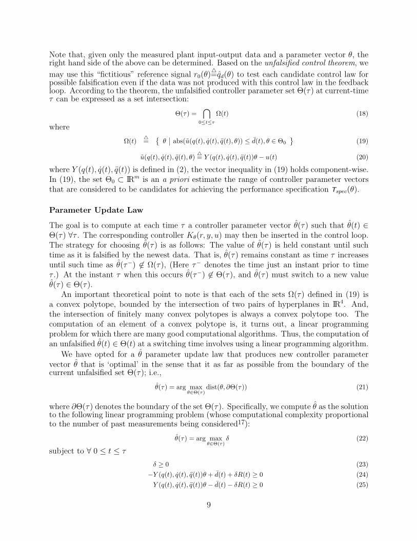
Note that, given only the measured plant input-output data and a parameter vector θ, theright hand side of the above can be determined. Based on the unfalsified control theorem, wemay use this “fictitious” reference signal r0(θ)

4=qd(θ) to test each candidate control law forpossible falsification even if the data was not produced with this control law in the feedbackloop. According to the theorem, the unfalsified controller parameter set Θ(τ) at current-timeτ can be expressed as a set intersection:

Θ(τ) =⋂

0≤t≤τ

Ω(t) (18)

where

Ω(t)4=

θ abs(u(q(t), q(t), q(t), θ)) ≤ d(t), θ ∈ Θ0

(19)

u(q(t), q(t), q(t), θ)4= Y (q(t), q(t), q(t))θ − u(t) (20)

where Y (q(t), q(t), q(t)) is defined in (2), the vector inequality in (19) holds component-wise.In (19), the set Θ0 ⊂ IRm is an a priori estimate the range of controller parameter vectorsthat are considered to be candidates for achieving the performance specification Tspec(θ).

Parameter Update Law

The goal is to compute at each time τ a controller parameter vector θ(τ) such that θ(t) ∈Θ(τ) ∀τ . The corresponding controller Kθ(r, y, u) may then be inserted in the control loop.The strategy for choosing θ(τ) is as follows: The value of θ(τ) is held constant until suchtime as it is falsified by the newest data. That is, θ(τ) remains constant as time τ increasesuntil such time as θ(τ−) 6∈ Ω(τ), (Here τ− denotes the time just an instant prior to timeτ .) At the instant τ when this occurs θ(τ−) 6∈ Θ(τ), and θ(τ) must switch to a new valueθ(τ) ∈ Θ(τ).

An important theoretical point to note is that each of the sets Ω(τ) defined in (19) isa convex polytope, bounded by the intersection of two pairs of hyperplanes in IR4. And,the intersection of finitely many convex polytopes is always a convex polytope too. Thecomputation of an element of a convex polytope is, it turns out, a linear programmingproblem for which there are many good computational algorithms. Thus, the computation ofan unfalsified θ(t) ∈ Θ(t) at a switching time involves using a linear programming algorithm.

We have opted for a θ parameter update law that produces new controller parametervector θ that is ‘optimal’ in the sense that it as far as possible from the boundary of thecurrent unfalsified set Θ(τ); i.e.,

θ(τ) = arg maxθ∈Θ(τ)

dist(θ, ∂Θ(τ)) (21)

where ∂Θ(τ) denotes the boundary of the set Θ(τ). Specifically, we compute θ as the solutionto the following linear programming problem (whose computational complexity proportionalto the number of past measurements being considered17):

θ(τ) = arg maxθ∈Θ(τ)

δ (22)

subject to ∀ 0 ≤ t ≤ τ

δ ≥ 0 (23)

−Y (q(t), q(t), q(t))θ + d(t) + δR(t) ≥ 0 (24)

Y (q(t), q(t), q(t))θ − d(t)− δR(t) ≥ 0 (25)

9

where R(t) ∈ IR2 is given by

R(t)4=

[

‖Y1(q(t), q(t), q(t))‖‖Y2(q(t), q(t), q(t))‖

]

(26)

where Yi(·), (i = 1, 2) denotes i-th row of the matrix Y (·) defined by (2). Here the maximalδ, say δ, is the radius of the largest ball that fits inside the convex polytope Θ(τ) and θ is itscenter. That is, θ is a point in Θ(τ) that is as far as possible from ∂Θ(τ) and δ the distanceof θ from ∂Θ(τ).

Besides the batch-type approach linear programming (22), a recursive algorithm for (22)is also possible because the unfalsified controller parameter set Θ(τ) is the intersection ofdegenerate ellipsoids (regions between “parallel” hyper planes), the recursive algorithm ofminimal-volume outer approximation by Fogel and Huang18 can be useful for the calculationof the intersections.

5 Computer SimulationSimulations are performed to demonstrate the performance of the unfalsified control method.The two-link manipulator example of Slotine et al. described in Section 2 is used in thesimulations; furthermore, in order to test the robustness capability of the unfalsified controlmethod, first order transfer functions of different bandwidth are used to simulate the actuatordynamics, viz.,

Ga(s) =1

τs + 1

where 1/(2πτ) is the actuator bandwidth in hertz; the values τ = 0, τ = 1/(10π) andτ = 1/(40π) were used in the simulations and displayed in the plots. In the simulation, thefollowing robot manipulator parameters are used

m1 = 1, l1 = 1, me = 2, δe = 30,

I1 = .12, lc1 = .5, Ie = 0.25, lce = 0.6

so that the exact parameter vector (in the absence of actuator) is θ∗ 4= [θ1, θ2, θ3, θ4]T =[3.34, 0.97, 1.0392, 0.6]T . The scenario of the simulation is that the end effector mass mechanges back and forth between 2 and 20 periodically with period 0.5 sec, so does its inertia Iebetween 0.25 and 2.5, so that the parameter vector changes between [3.34, 0.97, 1.0392, 0.6]Tand [30.07, 9.7, 10.3923, 6] periodically with period 0.5 sec accordingly. The magnitudes ofparameter vectors are unknown to the controller. The desired trajectory used is

qd1(t) = 30(1− cos 2πt), qd2(t) = 45(1− cos 2πt) .

The external torque disturbance acting on the two joints are sin 20πt and 2 sin 13πt, respec-tively. At time t = 0, the system is initially at rest with joint angles q1(0) = q2(0) = 0.4 rad.

For comparison, two control methods are examined. One is the unfalsified control method.The other is the adaptive control method by Slotine et al.19. The Slotine et al. controller is

u = Yslotθ + KD ˙q + Λq (27)

where θ is the estimated parameter vector of θ, KD is positive definite, and Λ is a positivedefinite matrix. Similar to (2), Yslot satisfies

H(θ, q)qr + C(θ, q, q)qr + g(θ, q) = Yslot(q, q, qr, qr)θ,

10

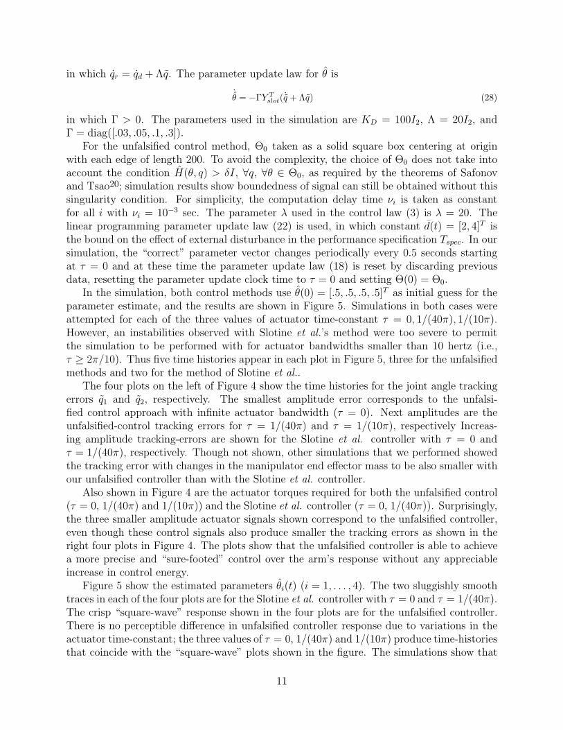
in which qr = qd + Λq. The parameter update law for θ is

˙θ = −ΓY Tslot( ˙q + Λq) (28)

in which Γ > 0. The parameters used in the simulation are KD = 100I2, Λ = 20I2, andΓ = diag([.03, .05, .1, .3]).

For the unfalsified control method, Θ0 taken as a solid square box centering at originwith each edge of length 200. To avoid the complexity, the choice of Θ0 does not take intoaccount the condition H(θ, q) > δI, ∀q, ∀θ ∈ Θ0, as required by the theorems of Safonovand Tsao20; simulation results show boundedness of signal can still be obtained without thissingularity condition. For simplicity, the computation delay time νi is taken as constantfor all i with νi = 10−3 sec. The parameter λ used in the control law (3) is λ = 20. Thelinear programming parameter update law (22) is used, in which constant d(t) = [2, 4]T isthe bound on the effect of external disturbance in the performance specification Tspec. In oursimulation, the “correct” parameter vector changes periodically every 0.5 seconds startingat τ = 0 and at these time the parameter update law (18) is reset by discarding previousdata, resetting the parameter update clock time to τ = 0 and setting Θ(0) = Θ0.

In the simulation, both control methods use θ(0) = [.5, .5, .5, .5]T as initial guess for theparameter estimate, and the results are shown in Figure 5. Simulations in both cases wereattempted for each of the three values of actuator time-constant τ = 0, 1/(40π), 1/(10π).However, an instabilities observed with Slotine et al.’s method were too severe to permitthe simulation to be performed with for actuator bandwidths smaller than 10 hertz (i.e.,τ ≥ 2π/10). Thus five time histories appear in each plot in Figure 5, three for the unfalsifiedmethods and two for the method of Slotine et al..

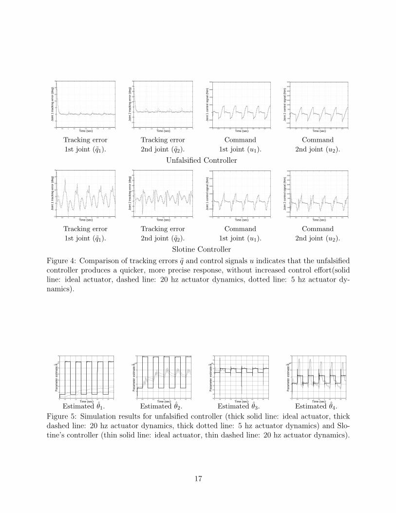
The four plots on the left of Figure 4 show the time histories for the joint angle trackingerrors q1 and q2, respectively. The smallest amplitude error corresponds to the unfalsi-fied control approach with infinite actuator bandwidth (τ = 0). Next amplitudes are theunfalsified-control tracking errors for τ = 1/(40π) and τ = 1/(10π), respectively Increas-ing amplitude tracking-errors are shown for the Slotine et al. controller with τ = 0 andτ = 1/(40π), respectively. Though not shown, other simulations that we performed showedthe tracking error with changes in the manipulator end effector mass to be also smaller withour unfalsified controller than with the Slotine et al. controller.

Also shown in Figure 4 are the actuator torques required for both the unfalsified control(τ = 0, 1/(40π) and 1/(10π)) and the Slotine et al. controller (τ = 0, 1/(40π)). Surprisingly,the three smaller amplitude actuator signals shown correspond to the unfalsified controller,even though these control signals also produce smaller the tracking errors as shown in theright four plots in Figure 4. The plots show that the unfalsified controller is able to achievea more precise and “sure-footed” control over the arm’s response without any appreciableincrease in control energy.

Figure 5 show the estimated parameters θi(t) (i = 1, . . . , 4). The two sluggishly smoothtraces in each of the four plots are for the Slotine et al. controller with τ = 0 and τ = 1/(40π).The crisp “square-wave” response shown in the four plots are for the unfalsified controller.There is no perceptible difference in unfalsified controller response due to variations in theactuator time-constant; the three values of τ = 0, 1/(40π) and 1/(10π) produce time-historiesthat coincide with the “square-wave” plots shown in the figure. The simulations show that

11

the Slotine et al. controller cannot accurately track the “correct” parameters. Attempts byus to improve this situation by adjusting Slotine’s parameter Γ proved unsuccessful.

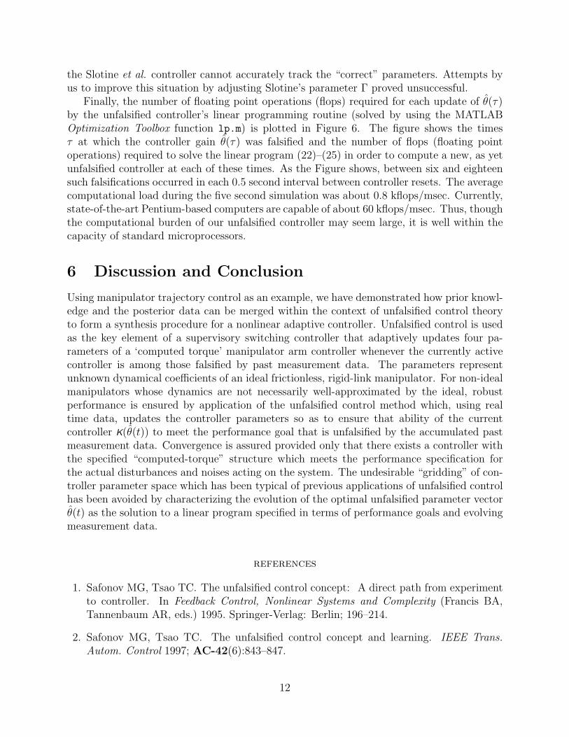
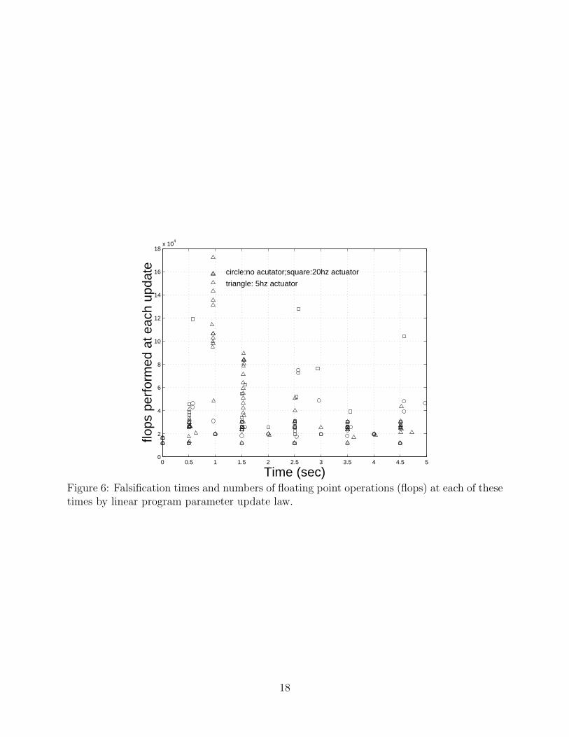
Finally, the number of floating point operations (flops) required for each update of θ(τ)by the unfalsified controller’s linear programming routine (solved by using the MATLABOptimization Toolbox function lp.m) is plotted in Figure 6. The figure shows the timesτ at which the controller gain θ(τ) was falsified and the number of flops (floating pointoperations) required to solve the linear program (22)–(25) in order to compute a new, as yetunfalsified controller at each of these times. As the Figure shows, between six and eighteensuch falsifications occurred in each 0.5 second interval between controller resets. The averagecomputational load during the five second simulation was about 0.8 kflops/msec. Currently,state-of-the-art Pentium-based computers are capable of about 60 kflops/msec. Thus, thoughthe computational burden of our unfalsified controller may seem large, it is well within thecapacity of standard microprocessors.

6 Discussion and Conclusion

Using manipulator trajectory control as an example, we have demonstrated how prior knowl-edge and the posterior data can be merged within the context of unfalsified control theoryto form a synthesis procedure for a nonlinear adaptive controller. Unfalsified control is usedas the key element of a supervisory switching controller that adaptively updates four pa-rameters of a ‘computed torque’ manipulator arm controller whenever the currently activecontroller is among those falsified by past measurement data. The parameters representunknown dynamical coefficients of an ideal frictionless, rigid-link manipulator. For non-idealmanipulators whose dynamics are not necessarily well-approximated by the ideal, robustperformance is ensured by application of the unfalsified control method which, using realtime data, updates the controller parameters so as to ensure that ability of the currentcontroller K(θ(t)) to meet the performance goal that is unfalsified by the accumulated pastmeasurement data. Convergence is assured provided only that there exists a controller withthe specified “computed-torque” structure which meets the performance specification forthe actual disturbances and noises acting on the system. The undesirable “gridding” of con-troller parameter space which has been typical of previous applications of unfalsified controlhas been avoided by characterizing the evolution of the optimal unfalsified parameter vectorθ(t) as the solution to a linear program specified in terms of performance goals and evolvingmeasurement data.

references

1. Safonov MG, Tsao TC. The unfalsified control concept: A direct path from experimentto controller. In Feedback Control, Nonlinear Systems and Complexity (Francis BA,Tannenbaum AR, eds.) 1995. Springer-Verlag: Berlin; 196–214.

2. Safonov MG, Tsao TC. The unfalsified control concept and learning. IEEE Trans.Autom. Control 1997; AC-42(6):843–847.

12

3. Brozenec TF, Safonov MG. Controller identification. In Proc. American ControlConf.,Albuquerque, NM, June 4–6, 1997; 2093–2097.

4. Kosut RL. Adaptive uncertainty modeling: On-line robust control design. In Proc.American Control Conf., Minneapolis, MN, June 1987; 245–250.

5. Kosut RL, Lau MK, Boyd SP. Set-membership identification of systems with parametricand nonparametric uncertainty. IEEE Trans. Autom. Control 1992; AC-37(7):929–941.

6. Krause JM. Stability margins with real parameter uncertainty: Test data implications.In Proc. American Control Conf., Pittsburgh, PA, June 21-23, 1989; 1441–1445.

7. Poolla K, Khargonekar P, Krause J, Tikku A, Nagpal K. A time-domain approach tomodel validation. IEEE Trans. Autom. Control 1994; AC-39(5):951–959.

8. Cabral FB, Safonov MG. Robustness oriented controller identification. In Proc. IFACSymp. on Robust Control Design, ROCOND ’97, Budapest, Hungary, June 25-27, 1997;113–118.

9. Willems JC. Paradigms and puzzles in the theory of dynamical systems. IEEE Trans.Autom. Control 1991, AC-36(3):259–294.

10. Slotine JJE., Li W. Applied Nonlinear Control 1991. Prentice-Hall: Englewood-Cliffs,NJ.

11. Luh JYS, Walker MW, Paul RPC. Resolved-acceleration control of mechanical manip-ulators. IEEE Trans. Autom. Control 1980; AC-25(3):468–474.

12. Mitchell T. Version spaces: A candidate elimination approach to rule learning. In Proc.Fifth Int. Joint Conf. on AI 1977. MIT Press: Cambridge, MA; 305–310.

13. Mitchell T. Machine Learning. McGraw-Hill: New York, 1997.

14. Sandberg IW. On the L2-boundedness of solutions of nonlinear functional equations.Bell System Technical Journal 1964, 43(4):1581–1599.

15. Zames G. On the input–output stability of time-varying nonlinear feedback systems —Part I: Conditions derived using concepts of loop gain, conicity and positivity. IEEETrans. Autom. Control 1966, AC-11(2):228–238.

16. Cabral FB, Safonov MG. A falsification perspective on model reference adaptive control.In Proc. IEEE Conf. on Decision and Control, Kobe, Japan, December 11–13, 1996;2982–2985.

17. Vicino A, Milanese M. Optimal inner bounds of feasible parameter set in linear estima-tion with bounded noise. IEEE Trans. Autom. Control 1991; AC-36(6):759–763.

18. Fogel E, Huang YF. On the value of information in system identification–bounded noisecase. Automatica 1982; 18(2):229–238.

13

19. Slotine JJE, Li W. Adaptive manipulator control: A case study. IEEE Trans. Autom.Control 1988; AC-33(11):995–1003.

20. Tsao TC, Safonov MG. Adaptive robust manipulator trajectory control — An applica-tion of unfalsified control method. In Proc. Fourth International Conference on Control,Automation, Robotics and Vision, Singapore, December 3–6, 1996.

14

List of Figures

1 A two-link robot manipulator with joint angles q1(t) and q2(t). . . . . . . . . 162 Computed torque manipulator control configuration. . . . . . . . . . . . . . 163 Feedback control system. . . . . . . . . . . . . . . . . . . . . . . . . . . . . . 164 Comparison of tracking errors q and control signals u indicates that the unfal-

sified controller produces a quicker, more precise response, without increasedcontrol effort(solid line: ideal actuator, dashed line: 20 hz actuator dynamics,dotted line: 5 hz actuator dynamics). . . . . . . . . . . . . . . . . . . . . . . 17

5 Simulation results for unfalsified controller (thick solid line: ideal actuator,thick dashed line: 20 hz actuator dynamics, thick dotted line: 5 hz actuatordynamics) and Slotine’s controller (thin solid line: ideal actuator, thin dashedline: 20 hz actuator dynamics). . . . . . . . . . . . . . . . . . . . . . . . . . 17

6 Falsification times and numbers of floating point operations (flops) at each ofthese times by linear program parameter update law. . . . . . . . . . . . . . 18

15

abc

q1

q2

Figure 1: A two-link robot manipulator with joint angles q1(t) and q2(t).

!

#"$&%(')+*-,."'0/123"*4/ , $&5 67980:<;

=?> "@)A' >CB#$A)AD*E) > '5F :@GHJI3KL:HJKLG MON

P PEQHRPF

S

TF F

S

U 8WVCX P ; FF RYY 7 YMT

Z[, 5\)AD4'^]*4"$&%_5`F H H F M

aHH

U 8bVCX P ;-cP HJde8WVCX P XfP ;fP Hhg8WVCX P ;

Figure 2: Computed torque manipulator control configuration.

Figure 3: Feedback control system.

16

0 0.5 1 1.5 2 2.5 3 3.5 4 4.5 5−10

−5

0

5

10

15

20

25

Time (sec)

Join

t 1 tr

acki

ng e

rror

(de

g)

0 0.5 1 1.5 2 2.5 3 3.5 4 4.5 5−15

−10

−5

0

5

10

15

20

25

30

Time (sec)Jo

int 2

trac

king

err

or (

deg)

0 0.5 1 1.5 2 2.5 3 3.5 4 4.5 5−4000

−2000

0

2000

4000

6000

8000

Time (sec)

Join

t 1 c

ontr

ol s

igna

l (N

m)

0 0.5 1 1.5 2 2.5 3 3.5 4 4.5 5−1500

−1000

−500

0

500

1000

1500

2000

2500

3000

3500

Time (sec)

Join

t 2 c

ontr

ol s

igna

l (N

m)

Tracking error Tracking error Command Command1st joint (q1). 2nd joint (q2). 1st joint (u1). 2nd joint (u2).

Unfalsified Controller

0 0.5 1 1.5 2 2.5 3 3.5 4 4.5 5−10

−5

0

5

10

15

20

25

Time (sec)

Join

t 1 tr

acki

ng e

rror

(de

g)

0 0.5 1 1.5 2 2.5 3 3.5 4 4.5 5−15

−10

−5

0

5

10

15

20

25

30

Time (sec)

Join

t 2 tr

acki

ng e

rror

(de

g)

0 0.5 1 1.5 2 2.5 3 3.5 4 4.5 5−4000

−2000

0

2000

4000

6000

8000

Time (sec)

Join

t 1 c

ontr

ol s

igna

l (N

m)

0 0.5 1 1.5 2 2.5 3 3.5 4 4.5 5−1500

−1000

−500

0

500

1000

1500

2000

2500

3000

3500

Time (sec)

Join

t 2 c

ontr

ol s

igna

l (N

m)

Tracking error Tracking error Command Command1st joint (q1). 2nd joint (q2). 1st joint (u1). 2nd joint (u2).

Slotine ControllerFigure 4: Comparison of tracking errors q and control signals u indicates that the unfalsifiedcontroller produces a quicker, more precise response, without increased control effort(solidline: ideal actuator, dashed line: 20 hz actuator dynamics, dotted line: 5 hz actuator dy-namics).

0 0.5 1 1.5 2 2.5 3 3.5 4 4.5 50

5

10

15

20

25

30

35

Time (sec)

Par

amet

er e

stim

ate

θ^1

0 0.5 1 1.5 2 2.5 3 3.5 4 4.5 5−2

0

2

4

6

8

10

Time (sec)

Par

amet

er e

stim

ate

θ^2

0 0.5 1 1.5 2 2.5 3 3.5 4 4.5 5−60

−50

−40

−30

−20

−10

0

10

20

30

40

Time (sec)

Par

amet

er e

stim

ate

θ^3

0 0.5 1 1.5 2 2.5 3 3.5 4 4.5 5−10

−5

0

5

10

15

20

Time (sec)

Par

amet

er e

stim

ate

θ^4

Estimated θ1. Estimated θ2. Estimated θ3. Estimated θ4.Figure 5: Simulation results for unfalsified controller (thick solid line: ideal actuator, thickdashed line: 20 hz actuator dynamics, thick dotted line: 5 hz actuator dynamics) and Slo-tine’s controller (thin solid line: ideal actuator, thin dashed line: 20 hz actuator dynamics).

17

0 0.5 1 1.5 2 2.5 3 3.5 4 4.5 50

2

4

6

8

10

12

14

16

18x 10

4

Time (sec)

flops

per

form

ed a

t eac

h up

date circle:no acutator;square:20hz actuator

triangle: 5hz actuator

Figure 6: Falsification times and numbers of floating point operations (flops) at each of thesetimes by linear program parameter update law.

18