Slides 11

Debraj Ray

Columbia, Fall 2013

Introduction

The salience of ethnic conflict

Inequality and polarization

Conflict and distribution: theory

Conflict and distribution: empirics

Future directions

0-0

Uneven Growth and the Social Backlash

Roots

Divergence (increasing returns, imperfect credit markets)

Sectoral change (agriculture/industry, domestic/exports)

Globalization (sectors with comparative advantage)

Reactions

Occupational choice (slow, imprecise, intergenerational)

Cross-sector percolation (demand patterns, inflation)

Political economy (person-based votes, wealth-based lobbying )

Conflict (Hirschman’s Tunnel)

0-1

The Ubiquity of Ethnic Conflict

WWII ! 22 inter-state conflicts.

9 killed more than 1000. Battle deaths 3–8m.

240 civil conflicts, 30 ongoing in 2010.

Half killed more than 1000. Battle deaths 5–10m.

Mass assassination of up to 25m civilians, 40 m displaced.

Does not count displacement and disease (est. 4x violent deaths).

0-2

0

10

20

30

40

50

1946 1951 1956 1961 1966 1971 1976 1981 1986 1991 1996 2001 2006

Intrastate

Internationalized Intrastate

Interstate

Colonial

Num

ber o

f Con

flict

s

0-3

Majority of these conflicts are ethnic Doyle-Sambanis (2000)

1945–1998, 100 of 700 known ethnic groups participated inrebellion Fearon (2006)

“In much of Asia and Africa, it is only modest hyperbole toassert that the Marxian prophecy has had an ethnic fulfillment.”Horowitz (1985)

Brubaker and Laitin (1998) on “eclipse of the left-right ideo-logical axis”

Fearon (2006), 1945–1998, approx. 700 ethnic groups known,over 100 of which participated in rebellions against the state.

0-4

The Salience Question

Uneven growth �! conflict, but along what lines?

Religion, ethnicity, geography, occupation, class?

The Marxian answer:

class

example: Maoist violence in rural India

But the argument is problematic.

Conflict is usually over directly contested resources.

0-5

Directly Contested Resources

Labor markets

Ethnic or racial divisions, immigrant vs native

Agrarian land

Rwanda, Darfur, Chattisgarh

Real estate

Gujarat, Bengal

Business resources

Kyrgystan, Ivory Coast, Malaysia . . .

0-6

Contestation ) conflict between economically similar groups

Some counterarguments:

bauxite/land in Maoist violence

agrarian/industrial land in Singur and Nandigram.

) class violence, but exception rather than the rule.

The implications of direct contestation:

Ethnic markers.

Instrumentalism as opposed to primordialism (Huntington, Lewis)

0-7

Do Ethnic Divisions Matter?

Two ways to approach this question.

Historical study of conflicts, one by one.

Bit of a wood-for-the-trees problem.

Horowitz (1985) summarizes some of the complexity:

“In dispersed systems, group loyalties are parochial, and ethnic con-flict is localized . . . A centrally focused system [with few groupings]possesses fewer cleavages than a dispersed system, but those itpossesses run through the whole society and are of greater magni-tude. When conflict occurs, the center has little latitude to placatesome groups without antagonizing others.”

0-8

Statistical approach

(Collier-Hoe✏er, Fearon-Laitin, Miguel-Satyanath-Sergenti)

Typical variables for conflict: demonstrations, processions, strikes,riots, casualties and on to civil war.

Explanatory variables:

Economic. per-capita income, inequality, resource holdings . . .

Geographic. mountains, separation from capital city . . .

Political. “democracy”, prior war . . .

And, of course, Ethnic. But how measured?

0-9

Information on ethnolinguistic diversity from:

World Christian Encyclopedia

Encyclopedia Britannica

Atlas Narodov Mira

CIA FactBook

Or religious diversity from:

L’Etat des Religions dans le Monde

World Christian Encyclopedia

The Statesman’s Yearbook

0-10

Fractionalization

Fractionalization index widely used:

F =mX

j=1

nj(1� nj)

where nj is population share of group j.

Special case of the Gini coe�cient

G =mX

j=1

MX

k=1

njnk�ik

where �ik is a notion of distance across groups.

0-11

Fractionalization used in many di↵erent contexts:

growth, governance, public goods provision.

But it shows no correlation with conflict.

See Collier and Hoe✏er (2002), Fearon and Laitin (2003),Miguel-Satyanath-Sergenti (2004).

Fearon and Laitin (APSR 2003)

“The estimates for the e↵ect of ethnic and religious fractionaliza-

tion are substantively and statistically insignificant . . . The empir-ical pattern is thus inconsistent with . . . the common expectationthat ethnic diversity is a major and direct cause of civil violence.”

0-12

And yet . . . fractionalization does not seem to capture theHorowitz quote:

“In dispersed systems, group loyalties are parochial, and ethnicconflict is localized . . . A centrally focused system [with few group-ings] possesses fewer cleavages than a dispersed system, but thoseit possesses run through the whole society and are of greater mag-nitude.”

Motivates the use of polarization measures by Montalvo andReynal-Querol (2005).

Based on a measure of polarization introduced by Esteban andRay (1994) and Duclos, Esteban and Ray (2003)

0-13

The Identity-Alienation Framework

Society is divided into “groups” (economic, social, religious,spatial...)

Identity. There is “homogeneity” within each group.

Alienation. There is “heterogeneity” across groups.

Esteban and Ray (1994) presumed that such a situation isconflictual:

“We begin with the obvious question: why are we interested inpolarization? It is our contention that the phenomenon of po-larization is closely linked to the generation of tensions, to thepossibilities of articulated rebellion and revolt, and to the existenceof social unrest in general . . . ”

0-14

Measuring Polarization

(adapted from Duclos, Esteban and Ray, 2003)

Space of densities (cdfs) on income, political opinion, etc.

Each individual located at “income” x feels

Identification with people of “similar” income (the height ofdensity n(x) at point x.)

Alienation from people with “dissimilar” income (the incomedistance |y� x| of y from x.)

E↵ective Antagonism of x towards y depends on x’s alienationfrom y and on x’s sense of identification.

T (i, a)

where i = n(x) and a = |x� y|.

0-15

View polarization as the “sum” of all such antagonisms

P (f ) =Z Z

T (n(x), |x� y|)n(x)n(y)dxdy

Not very useful as it stands. Axioms to narrow down P .

Based on special distributions, built from uniform kernels.

Income or Wealth

0-16

Axiom 1. If a distribution is just a single uniform density, a“global compression” cannot increase polarization.

Income or Wealth

0-17

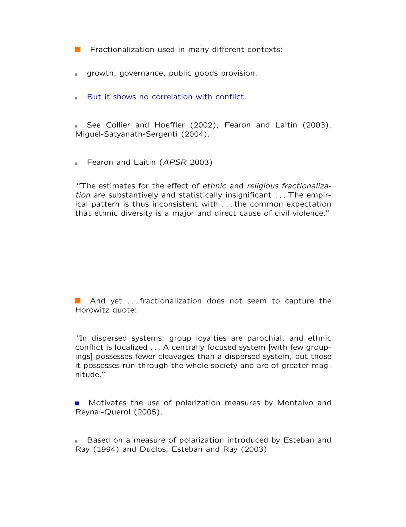
Axiom 2. If a symmetric distribution is composed of threeuniform kernels, then a compression of the side kernels cannotreduce polarization.

Income or Wealth

0-18

Axiom 3. If a symmetric distribution is composed of four uni-form kernels, then a symmetric slide of the two middle kernels awayfrom each other must increase polarization.

Income or Wealth

0-19

Axiom 4. [Population Neutrality.] Polarization comparisons areunchanged if both populations are scaled up or down by the samepercentage.

Theorem. A polarization measure satisfies Axioms 1–4 if andonly if it is proportional to

Z Zn(x)1+↵n(y)|y� x|dydx,

where ↵ lies between 0.25 and 1.

Compare with the Gini coe�cient / fractionalization index:

Gini =Z Z

n(x)n(y)|y� x|dydx,

It’s ↵ that makes all the di↵erence.

0-20

Some Properties

1. Not Inequality. See Axiom 2.

2. Bimodal. Polarization maximal for bimodal distributions,but defined of course over all distributions.

0-21

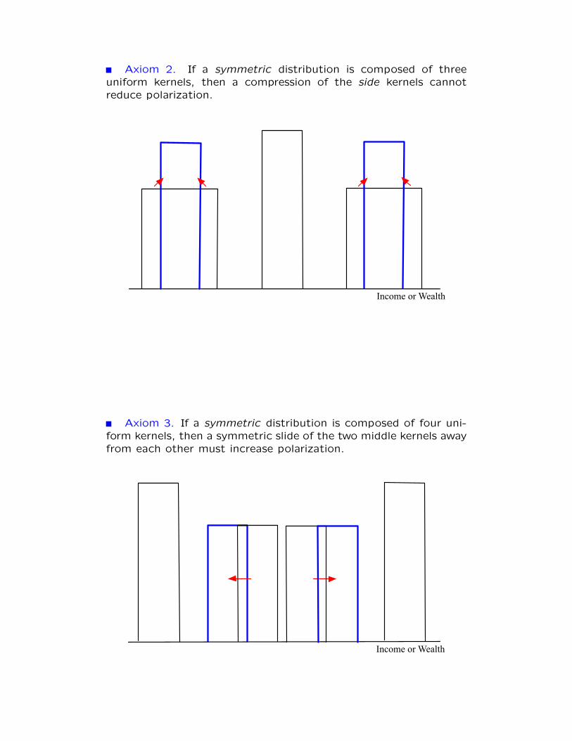
3. Global. The local “merger” of two groups has e↵ects thatdepend on the shape of the distribution elsewhere.

Income

Density

0-22

3. Global, contd. Compare previous merger with this one.

Income

Density

0-23

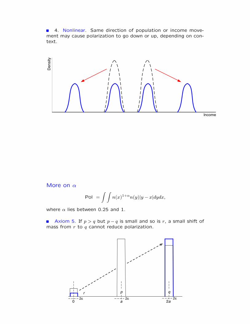
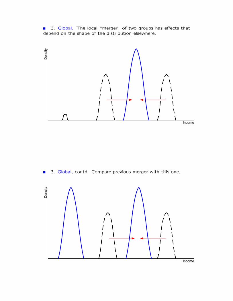
4. Nonlinear. Same direction of population or income move-ment may cause polarization to go down or up, depending on con-text.

Income

Density

0-24

More on ↵

Pol =Z Z

n(x)1+↵n(y)|y� x|dydx,

where ↵ lies between 0.25 and 1.

Axiom 5. If p > q but p� q is small and so is r, a small shift ofmass from r to q cannot reduce polarization.

r p q

0 a 2a2ε 2ε 2ε

0-25

Theorem. Under the additional Axiom 5, it must be that ↵ = 1,so the unique polarization measure that satisfies the five axioms isproportional to Z Z

n(x)2n(y)|y� x|dydx.

Easily applicable to ethnolinguistic or religious groupings.

Say m “social groups”, nj is population proportion in group j.

If all inter-group distances are binary, then

Pol =MX

j=1

MX

k=1

n2jnk =

MX

j=1

n2j (1� nj).

Compare with F =MX

j=1

nj(1� nj).

0-26

Polarization and Conflict: Behavior

Axiomatics suggest (but cannot establish) a link between po-larization and conflict.

Two approaches:

Theoretical. Write down a “natural” theory which links conflictwith these measures.

Empirical.Take the measures to the data and see they are re-lated to conflict.

We discuss the theory first (based on Esteban and Ray, 2011).

0-27

A Model of Conflict

m groups engaged in conflict.

Ni in group i,Pm

i=1 Ni = N .

Ri is total contribution of resources by group i.

R =mX

i=1

Ri.

R/N is a measure of overall conflict.

Probability that group i wins the conflict is given by

pi =Ri

R

Cost c(ri): quadratic spec (1/2)r2i , more generally (1/✓)r✓i .

0-28

Win and lose payo↵s: public and private components.

Public prize:

(religious dominance, political control, hatreds, public goods)

weight �, uij is payo↵ matrix.

Private prize

(oil, diamonds, scarce land)

weight 1� �, per-capita (1� �)/n

Net expected payo↵ per-capita to person k in group i is

Yi(k) =mX

j=1

pj�uij + pi(1� �)

ni� c (ri) .

pub priv cost

0-29

How do Individuals Make Contributions?

One extreme: individuals maximize own payo↵.

Another extreme: there is full intra-group cohesion and individ-ual contributions maximize group payo↵s.

Intermediate situations: define person k’s extended utility by

Ui(k) ⌘ (1� ↵)Yi(k) + ↵X

`2i

Yi(`),

where ↵ lies between 0 and 1. (Sen 1964)

Interpretations for ↵: (i) intragroup concern or altruism (ii)group cohesion.

0-30

Equilibrium

A collection {ri(k)} of individual contributions where for everygroup i and member k, ri(k) maximizes

(1� ↵)Yi(k) + ↵X

`2i

Yi(`)

which is the same as maximizing

[(1� ↵) + ↵Ni]

2

4�mX

j=1

pjuij + pi1� �

ni

3

5� c(ri(k)).

given the contributions of everyone else.

Theorem. An equilibrium always exists and it is unique.

0-31

Simplify above maximization problem. Define:

�i ⌘ (1� ↵) + ↵Ni

�ij ⌘ uii � uij distances

Dii ⌘ 0, and Dij ⌘ ��ij + (1� �)/ni for all j 6= i.

So maximize

��i

mX

j=1

pjDij � c(ri(k))

First-order condition with respect to ri(k):

�i

R

mX

j=1

pjDij = c0(ri(k))

for all k, which means that ri(k) = ri for all i, so that:

�i

R

mX

j=1

pjDij = c0(ri).

0-32

The solution to this is hard to find in closed form.

Example: quadratic cost c(r) = (1/2)r2; then

1� ↵

N+ ↵ni

� mX

j=1

pjDij = ri⇢

where ⇢ ⌘ R/N is per-capita conflict.

Multiply both sides by ni and take N ! 1 to set up the system:

mX

j=1

pjn2i Dij = pi⇢

2

Let W be m⇥m matrix with n2i Dij as element. Then

Wp = ⇢2p.

⇢2 is the unique positive eigenvalue of W

p is the associated eigenvector on unit simplex.

0-33

Return to general case. Manipulate FOC to get:

1

N

mX

j=1

pipj�iDij = ⇢pic0(ri)

Define correction factors �i ⌘ pi/ni. Rewrite some more:

1

N

mX

j=1

�i�jninj�iDij = ⇢pic0(�i⇢)

Multiply both sides by c0(⇢)/c0(�i⇢), sum over all i:

mX

i=1

mX

j=1

�(�i, �j , ⇢)ninj�iDij

N= ⇢

mX

i=1

pic0(⇢) = ⇢c0(⇢),

where

�(�i, �j , ⇢) ⌘c0(⇢)�i�jc0(�i⇢)

.

0-34

Ignore the � term (which is 1 when all � equal 1):

⇢c0(⇢) 'mX

i=1

mX

j=1

ninj�iDij

N

Start opening up the �i’s and the Dij’s:

⇢c0(⇢) 'mX

i=1

X

j 6=i

ninj[(1� ↵) + ↵Ni][��ij + (1� �)/ni]

N

= !1 + !2G+ ↵[�P + (1� �)F ]

where

P =mX

i=1

mX

j=1

n2inj�ij ,

F =mX

i=1

ni(1� ni),

G =mX

i=1

mX

j=1

ninj�ij .

0-35

Approximation Theorem

Theorem. Neglect joint impact of the deviation of correctionfactors from unity. Then the per-capita cost of conflict is approx-imately ⇢̂, given by

⇢̂c0(⇢̂) = !1 + !2G+ ↵[�P + (1� �)F ],

where

!1 ⌘ (1� �)(1� ↵)(m� 1)/N

!2 ⌘ �(1� ↵)/N .

and G, P and F are as defined earlier.

For large N : only P and F matter if ↵ > 0:

⇢̂c0(⇢̂) ' ↵[�P + (1� �)F ]

0-36

How Good is the Approximation?

Holds exactly when there are just two groups and all goods arepublic.

Holds exactly when all groups the same size and public goodslosses are symmetric.

Holds almost exactly for contests when conflict is high enough.

Can numerically simulate to see how good the approximationis.

0-37

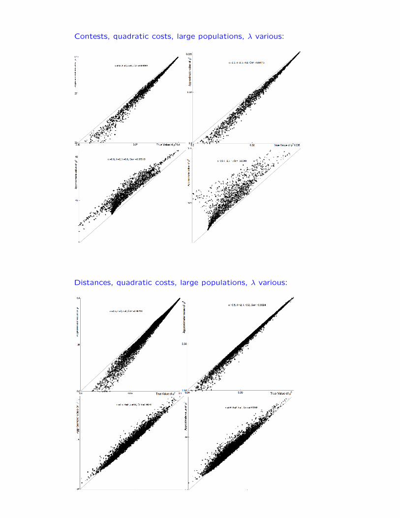
Contests, quadratic costs, large populations, � various:

0-38

Distances, quadratic costs, large populations, � various:

0-39

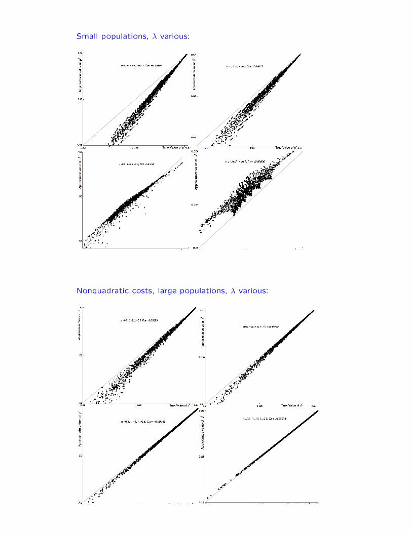
Small populations, � various:

0-40

Nonquadratic costs, large populations, � various:

0-41

Empirical Investigation

(Esteban, Mayoral and Ray AER 2012, Science 2012)

138 countries over 1960–2008 (pooled cross-section).

prio25: 25+ battle deaths in the year. [Baseline]

priocw: prio25 + total exceeding 1000 battle-related deaths.

prio1000: 1,000+ battle-related deaths in the year.

prioint: weighted combination of above.

isc: Continuous index, Banks (2008), weighted average of 8di↵erent manifestations of coflict.

0-42

Groups

Fearon database: “culturally distinct” groups in 160 countries.

based on ethnolinguistic criteria.

Ethnologue: information on linguistic groups.

Ethnologue 6,912 living languages + group sizes.

0-43

Preferences and Distances

We use linguistic distances on language trees.

E.g., all Indo-European languages in common subtree.

Spanish and Basque diverge at the first branch; Spanish andCatalan share first 7 nodes. Max: 15 steps of branching.

Similarity sij = common branchesmaximal branches down that subtree.

Distance ij = 1� s�ij, for some � 2 (0, 1].

Baseline � = 0.05 as in Desmet et al (2009).

0-44

Additional Variables and Controls

Among the controls:

Population

GDP per capita

Dependence on oil

Mountainous terrain

Democracy

Governance, civil rights

Also:

Indices of publicness and privateness of the prize

Estimates of group concern from World Values Survey

0-45

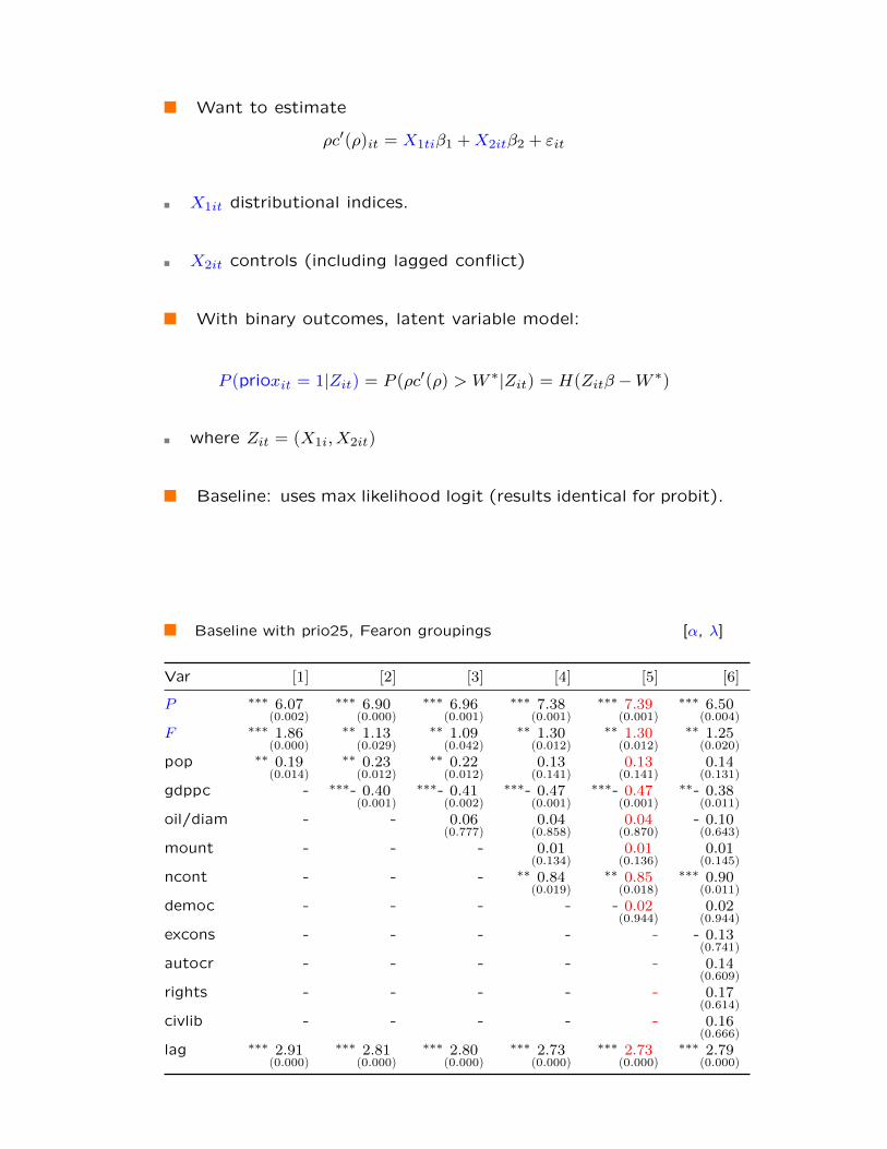
Want to estimate

⇢c0(⇢)it = X1ti�1 +X2it�2 + "it

X1it distributional indices.

X2it controls (including lagged conflict)

With binary outcomes, latent variable model:

P (prioxit = 1|Zit) = P (⇢c0(⇢) > W ⇤|Zit) = H(Zit� �W ⇤)

where Zit = (X1i,X2it)

Baseline: uses max likelihood logit (results identical for probit).

p-values use robust standard errors adjusted for clustering.

0-46

Baseline with prio25, Fearon groupings [↵, �]

Var [1] [2] [3] [4] [5] [6]

P ⇤⇤⇤ 6.07(0.002)

⇤⇤⇤ 6.90(0.000)

⇤⇤⇤ 6.96(0.001)

⇤⇤⇤ 7.38(0.001)

⇤⇤⇤ 7.39(0.001)

⇤⇤⇤ 6.50(0.004)

F ⇤⇤⇤ 1.86(0.000)

⇤⇤ 1.13(0.029)

⇤⇤ 1.09(0.042)

⇤⇤ 1.30(0.012)

⇤⇤ 1.30(0.012)

⇤⇤ 1.25(0.020)

pop ⇤⇤ 0.19(0.014)

⇤⇤ 0.23(0.012)

⇤⇤ 0.22(0.012)

0.13(0.141)

0.13(0.141)

0.14(0.131)

gdppc - ⇤⇤⇤- 0.40(0.001)

⇤⇤⇤- 0.41(0.002)

⇤⇤⇤- 0.47(0.001)

⇤⇤⇤- 0.47(0.001)

⇤⇤- 0.38(0.011)

oil/diam - - 0.06(0.777)

0.04(0.858)

0.04(0.870)

- 0.10(0.643)

mount - - - 0.01(0.134)

0.01(0.136)

0.01(0.145)

ncont - - - ⇤⇤ 0.84(0.019)

⇤⇤ 0.85(0.018)

⇤⇤⇤ 0.90(0.011)

democ - - - - - 0.02(0.944)

0.02(0.944)

excons - - - - - - 0.13(0.741)

autocr - - - - - 0.14(0.609)

rights - - - - - 0.17(0.614)

civlib - - - - - 0.16(0.666)

lag ⇤⇤⇤ 2.91(0.000)

⇤⇤⇤ 2.81(0.000)

⇤⇤⇤ 2.80(0.000)

⇤⇤⇤ 2.73(0.000)

⇤⇤⇤ 2.73(0.000)

⇤⇤⇤ 2.79(0.000)

0-47

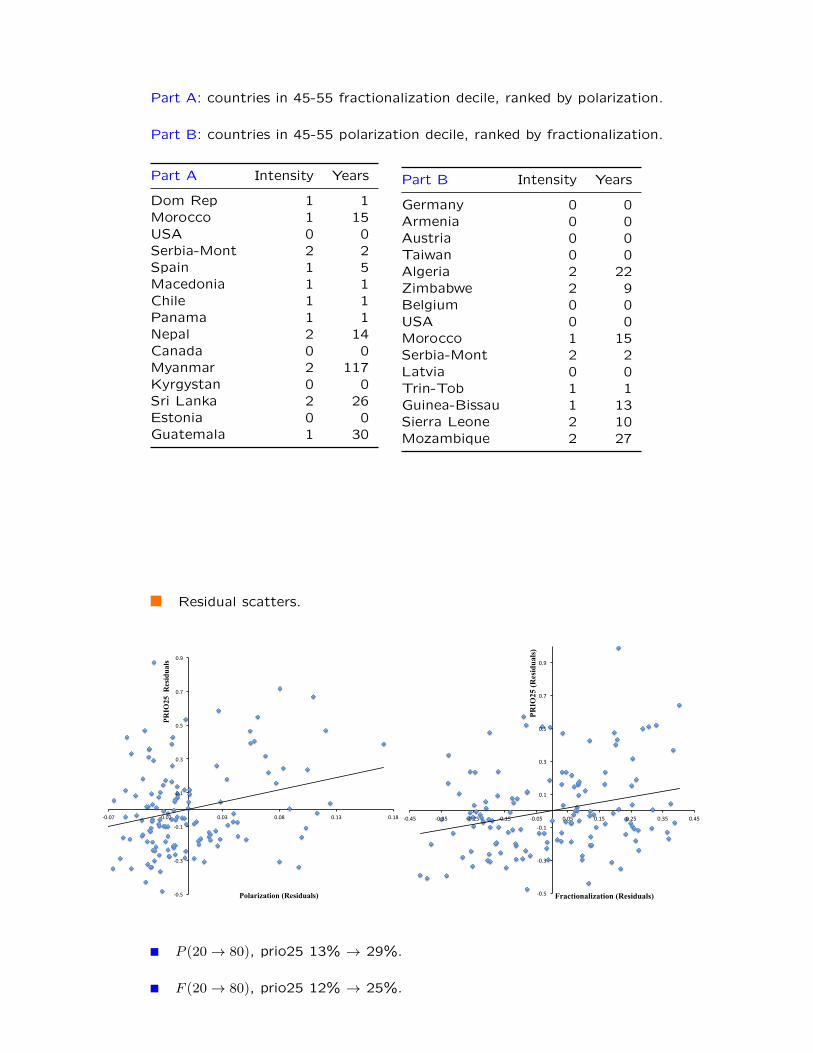
Part A: countries in 45-55 fractionalization decile, ranked by polarization.

Part B: countries in 45-55 polarization decile, ranked by fractionalization.

Part A Intensity Years

Dom Rep 1 1Morocco 1 15USA 0 0Serbia-Mont 2 2Spain 1 5Macedonia 1 1Chile 1 1Panama 1 1Nepal 2 14Canada 0 0Myanmar 2 117Kyrgystan 0 0Sri Lanka 2 26Estonia 0 0Guatemala 1 30

Part B Intensity Years

Germany 0 0Armenia 0 0Austria 0 0Taiwan 0 0Algeria 2 22Zimbabwe 2 9Belgium 0 0USA 0 0Morocco 1 15Serbia-Mont 2 2Latvia 0 0Trin-Tob 1 1Guinea-Bissau 1 13Sierra Leone 2 10Mozambique 2 27

0-48

Residual scatters.

!"#$%

!"#&%

!"#'%

"#'%

"#&%

"#$%

"#(%

"#)%

!"#"(% !"#"*% "#"&% "#"+% "#'&% "#'+%

PRIO

25 R

esid

uals

Polarization (Residuals) !"#$%

!"#&%

!"#'%

"#'%

"#&%

"#$%

"#(%

"#)%

!"#*$% !"#&$% !"#+$% !"#'$% !"#"$% "#"$% "#'$% "#+$% "#&$% "#*$%

PRIO

25 (R

esid

uals

)

Fractionalization (Residuals)

P (20 ! 80), prio25 13% ! 29%.

F (20 ! 80), prio25 12% ! 25%.

0-49

Robustness Checks

Alternative definitions of conflict

Alternative definition of groups: Ethnologue

Binary versus language-based distances

Conflict onset

Region and time e↵ects

Other ways of estimating the baseline model

0-50

Di↵erent definitions of conflict, Fearon groupings

Variable prio25 priocw prio1000 prioint isc

P ⇤⇤⇤ 7.39(0.001)

⇤⇤⇤ 6.76(0.007)

⇤⇤⇤ 10.47(0.001)

⇤⇤⇤ 6.50(0.000)

⇤⇤⇤ 25.90(0.003)

F ⇤⇤ 1.30(0.012)

⇤⇤ 1.39(0.034)

⇤ 1.11(0.086)

⇤⇤⇤ 1.30(0.006)

2.27(0.187)

gdp ⇤⇤⇤- 0.47(0.001)

⇤- 0.35(0.066)

⇤⇤⇤- 0.63(0.000)

⇤⇤⇤- 0.40(0.002)

⇤⇤⇤- 1.70(0.001)

pop 0.13(0.141)

⇤ 0.19(0.056)

0.13(0.215)

0.10(0.166)

⇤⇤⇤ 1.11(0.000)

oil/diam 0.04(0.870)

0.06(0.825)

- 0.03(0.927)

- 0.04(0.816)

- 0.57(0.463)

mount 0.01(0.136)

⇤⇤ 0.01(0.034)

0.01(0.323)

0.00(0.282)

⇤⇤ 0.04(0.022)

ncont ⇤⇤ 0.85(0.018)

0.62(0.128)

⇤ 0.78(0.052)

⇤ 0.55(0.069)

⇤⇤⇤ 4.38(0.004)

democ - 0.02(0.944)

- 0.09(0.790)

- 0.41(0.230)

- 0.03(0.909)

0.06(0.944)

lag ⇤⇤⇤ 2.73(0.000)

⇤⇤⇤ 3.74(0.000)

⇤⇤⇤ 2.78(0.000)

⇤⇤⇤ 2.00(0.000)

⇤⇤⇤ 0.50(0.000)

P (20 ! 80), prio25 13%–29%, priocw 7%–17%, prio1000 3%–10%.

F (20 ! 80), prio25 12%–25%, priocw 7%–16%, prio1000 3%–6%.

0-51

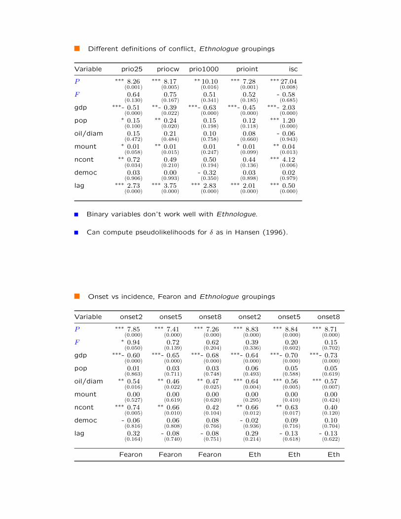
Di↵erent definitions of conflict, Ethnologue groupings

Variable prio25 priocw prio1000 prioint isc

P ⇤⇤⇤ 8.26(0.001)

⇤⇤⇤ 8.17(0.005)

⇤⇤ 10.10(0.016)

⇤⇤⇤ 7.28(0.001)

⇤⇤⇤ 27.04(0.008)

F 0.64(0.130)

0.75(0.167)

0.51(0.341)

0.52(0.185)

- 0.58(0.685)

gdp ⇤⇤⇤- 0.51(0.000)

⇤⇤- 0.39(0.022)

⇤⇤⇤- 0.63(0.000)

⇤⇤⇤- 0.45(0.000)

⇤⇤⇤- 2.03(0.000)

pop ⇤ 0.15(0.100)

⇤⇤ 0.24(0.020)

0.15(0.198)

0.12(0.118)

⇤⇤⇤ 1.20(0.000)

oil/diam 0.15(0.472)

0.21(0.484)

0.10(0.758)

0.08(0.660)

- 0.06(0.943)

mount ⇤ 0.01(0.058)

⇤⇤ 0.01(0.015)

0.01(0.247)

⇤ 0.01(0.099)

⇤⇤ 0.04(0.013)

ncont ⇤⇤ 0.72(0.034)

0.49(0.210)

0.50(0.194)

0.44(0.136)

⇤⇤⇤ 4.12(0.006)

democ 0.03(0.906)

0.00(0.993)

- 0.32(0.350)

0.03(0.898)

0.02(0.979)

lag ⇤⇤⇤ 2.73(0.000)

⇤⇤⇤ 3.75(0.000)

⇤⇤⇤ 2.83(0.000)

⇤⇤⇤ 2.01(0.000)

⇤⇤⇤ 0.50(0.000)

Binary variables don’t work well with Ethnologue.

Can compute pseudolikelihoods for � as in Hansen (1996).

0-52

Onset vs incidence, Fearon and Ethnologue groupings

Variable onset2 onset5 onset8 onset2 onset5 onset8

P ⇤⇤⇤ 7.85(0.000)

⇤⇤⇤ 7.41(0.000)

⇤⇤⇤ 7.26(0.000)

⇤⇤⇤ 8.83(0.000)

⇤⇤⇤ 8.84(0.000)

⇤⇤⇤ 8.71(0.000)

F ⇤ 0.94(0.050)

0.72(0.139)

0.62(0.204)

0.39(0.336)

0.20(0.602)

0.15(0.702)

gdp ⇤⇤⇤- 0.60(0.000)

⇤⇤⇤- 0.65(0.000)

⇤⇤⇤- 0.68(0.000)

⇤⇤⇤- 0.64(0.000)

⇤⇤⇤- 0.70(0.000)

⇤⇤⇤- 0.73(0.000)

pop 0.01(0.863)

0.03(0.711)

0.03(0.748)

0.06(0.493)

0.05(0.588)

0.05(0.619)

oil/diam ⇤⇤ 0.54(0.016)

⇤⇤ 0.46(0.022)

⇤⇤ 0.47(0.025)

⇤⇤⇤ 0.64(0.004)

⇤⇤⇤ 0.56(0.005)

⇤⇤⇤ 0.57(0.007)

mount 0.00(0.527)

0.00(0.619)

0.00(0.620)

0.00(0.295)

0.00(0.410)

0.00(0.424)

ncont ⇤⇤⇤ 0.74(0.005)

⇤⇤ 0.66(0.010)

0.42(0.104)

⇤⇤ 0.66(0.012)

⇤⇤ 0.63(0.017)

0.40(0.120)

democ - 0.06(0.816)

0.06(0.808)

0.08(0.766)

- 0.02(0.936)

0.09(0.716)

0.10(0.704)

lag 0.32(0.164)

- 0.08(0.740)

- 0.08(0.751)

0.29(0.214)

- 0.13(0.618)

- 0.13(0.622)

Fearon Fearon Fearon Eth Eth Eth

0-53

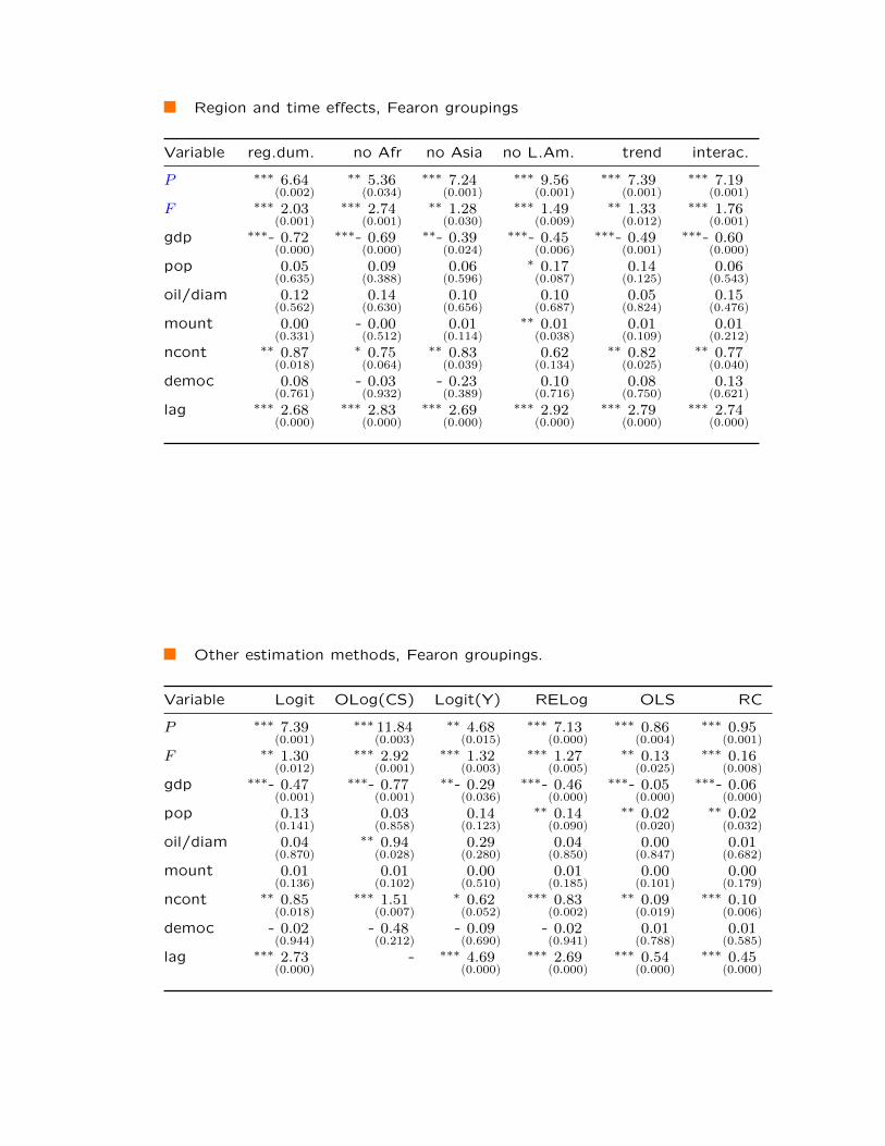
Region and time e↵ects, Fearon groupings

Variable reg.dum. no Afr no Asia no L.Am. trend interac.

P ⇤⇤⇤ 6.64(0.002)

⇤⇤ 5.36(0.034)

⇤⇤⇤ 7.24(0.001)

⇤⇤⇤ 9.56(0.001)

⇤⇤⇤ 7.39(0.001)

⇤⇤⇤ 7.19(0.001)

F ⇤⇤⇤ 2.03(0.001)

⇤⇤⇤ 2.74(0.001)

⇤⇤ 1.28(0.030)

⇤⇤⇤ 1.49(0.009)

⇤⇤ 1.33(0.012)

⇤⇤⇤ 1.76(0.001)

gdp ⇤⇤⇤- 0.72(0.000)

⇤⇤⇤- 0.69(0.000)

⇤⇤- 0.39(0.024)

⇤⇤⇤- 0.45(0.006)

⇤⇤⇤- 0.49(0.001)

⇤⇤⇤- 0.60(0.000)

pop 0.05(0.635)

0.09(0.388)

0.06(0.596)

⇤ 0.17(0.087)

0.14(0.125)

0.06(0.543)

oil/diam 0.12(0.562)

0.14(0.630)

0.10(0.656)

0.10(0.687)

0.05(0.824)

0.15(0.476)

mount 0.00(0.331)

- 0.00(0.512)

0.01(0.114)

⇤⇤ 0.01(0.038)

0.01(0.109)

0.01(0.212)

ncont ⇤⇤ 0.87(0.018)

⇤ 0.75(0.064)

⇤⇤ 0.83(0.039)

0.62(0.134)

⇤⇤ 0.82(0.025)

⇤⇤ 0.77(0.040)

democ 0.08(0.761)

- 0.03(0.932)

- 0.23(0.389)

0.10(0.716)

0.08(0.750)

0.13(0.621)

lag ⇤⇤⇤ 2.68(0.000)

⇤⇤⇤ 2.83(0.000)

⇤⇤⇤ 2.69(0.000)

⇤⇤⇤ 2.92(0.000)

⇤⇤⇤ 2.79(0.000)

⇤⇤⇤ 2.74(0.000)

0-54

Other estimation methods, Fearon groupings.

Variable Logit OLog(CS) Logit(Y) RELog OLS RC

P ⇤⇤⇤ 7.39(0.001)

⇤⇤⇤ 11.84(0.003)

⇤⇤ 4.68(0.015)

⇤⇤⇤ 7.13(0.000)

⇤⇤⇤ 0.86(0.004)

⇤⇤⇤ 0.95(0.001)

F ⇤⇤ 1.30(0.012)

⇤⇤⇤ 2.92(0.001)

⇤⇤⇤ 1.32(0.003)

⇤⇤⇤ 1.27(0.005)

⇤⇤ 0.13(0.025)

⇤⇤⇤ 0.16(0.008)

gdp ⇤⇤⇤- 0.47(0.001)

⇤⇤⇤- 0.77(0.001)

⇤⇤- 0.29(0.036)

⇤⇤⇤- 0.46(0.000)

⇤⇤⇤- 0.05(0.000)

⇤⇤⇤- 0.06(0.000)

pop 0.13(0.141)

0.03(0.858)

0.14(0.123)

⇤⇤ 0.14(0.090)

⇤⇤ 0.02(0.020)

⇤⇤ 0.02(0.032)

oil/diam 0.04(0.870)

⇤⇤ 0.94(0.028)

0.29(0.280)

0.04(0.850)

0.00(0.847)

0.01(0.682)

mount 0.01(0.136)

0.01(0.102)

0.00(0.510)

0.01(0.185)

0.00(0.101)

0.00(0.179)

ncont ⇤⇤ 0.85(0.018)

⇤⇤⇤ 1.51(0.007)

⇤ 0.62(0.052)

⇤⇤⇤ 0.83(0.002)

⇤⇤ 0.09(0.019)

⇤⇤⇤ 0.10(0.006)

democ - 0.02(0.944)

- 0.48(0.212)

- 0.09(0.690)

- 0.02(0.941)

0.01(0.788)

0.01(0.585)

lag ⇤⇤⇤ 2.73(0.000)

- ⇤⇤⇤ 4.69(0.000)

⇤⇤⇤ 2.69(0.000)

⇤⇤⇤ 0.54(0.000)

⇤⇤⇤ 0.45(0.000)

0-55

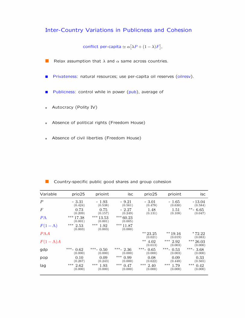
Inter-Country Variations in Publicness and Cohesion

conflict per-capita ' ↵⇥�P + (1� �)F

⇤,

Relax assumption that � and ↵ same across countries.

Privateness: natural resources; use per-capita oil reserves (oilresv).

Publicness: control while in power (pub), average of

Autocracy (Polity IV)

Absence of political rights (Freedom House)

Absence of civil liberties (Freedom House)

L ⌘ (pub*gdp)/(pub*gdp+ oilresv).

0-56

Country-specific public good shares and group cohesion

Variable prio25 prioint isc prio25 prioint isc

P - 3.31(0.424)

- 1.93(0.538)

- 9.21(0.561)

- 3.01(0.478)

- 1.65(0.630)

-13.04(0.584)

F 0.73(0.209)

0.75(0.157)

- 2.27(0.249)

1.48(0.131)

1.51(0.108)

⇤⇤- 6.65(0.047)

PL ⇤⇤⇤ 17.38(0.001)

⇤⇤⇤ 13.53(0.001)

⇤⇤⇤ 60.23(0.005)

F (1� L) ⇤⇤⇤ 2.53(0.003)

⇤⇤⇤ 1.92(0.003)

⇤⇤⇤ 11.87(0.000)

PLA ⇤⇤ 23.25(0.021)

⇤⇤ 19.16(0.019)

⇤ 72.22(0.083)

F (1� L)A ⇤⇤ 4.02(0.013)

⇤⇤⇤ 2.92(0.003)

⇤⇤⇤ 26.03(0.000)

gdp ⇤⇤⇤- 0.62(0.000)

⇤⇤⇤- 0.50(0.000)

⇤⇤⇤- 2.36(0.000)

⇤⇤⇤- 0.65(0.000)

⇤⇤⇤- 0.53(0.003)

⇤⇤⇤- 3.68(0.000)

pop 0.10(0.267)

0.09(0.243)

⇤⇤⇤ 0.99(0.000)

0.08(0.622)

0.09(0.448)

0.33(0.565)

lag ⇤⇤⇤ 2.62(0.000)

⇤⇤⇤ 1.93(0.000)

⇤⇤⇤ 0.47(0.000)

⇤⇤⇤ 2.40(0.000)

⇤⇤⇤ 1.79(0.000)

⇤⇤⇤ 0.42(0.000)

0-57

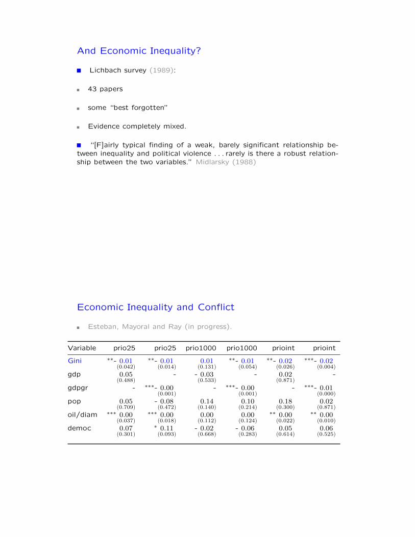
And Economic Inequality?

Lichbach survey (1989):

43 papers

some “best forgotten”

Evidence completely mixed.

“[F]airly typical finding of a weak, barely significant relationship be-tween inequality and political violence . . . rarely is there a robust relation-ship between the two variables.” Midlarsky (1988)

0-58

Economic Inequality and Conflict

Esteban, Mayoral and Ray (in progress).

Variable prio25 prio25 prio1000 prio1000 prioint prioint

Gini ⇤⇤- 0.01(0.042)

⇤⇤- 0.01(0.014)

0.01(0.131)

⇤⇤- 0.01(0.054)

⇤⇤- 0.02(0.026)

⇤⇤⇤- 0.02(0.004)

gdp 0.05(0.488)

- - 0.03(0.533)

- 0.02(0.871)

-

gdpgr - ⇤⇤⇤- 0.00(0.001)

- ⇤⇤⇤- 0.00(0.001)

- ⇤⇤⇤- 0.01(0.000)

pop 0.05(0.709)

- 0.08(0.472)

0.14(0.140)

0.10(0.214)

0.18(0.300)

0.02(0.871)

oil/diam ⇤⇤⇤ 0.00(0.037)

⇤⇤⇤ 0.00(0.018)

0.00(0.112)

0.00(0.124)

⇤⇤ 0.00(0.022)

⇤⇤ 0.00(0.010)

democ 0.07(0.301)

⇤ 0.11(0.093)

- 0.02(0.668)

- 0.06(0.283)

0.05(0.614)

0.06(0.525)

0-59

Surprising? Not Really

Two entry points:

Wealth of the rival group — related to the gains from conflict.

Wealth of the own group — related to the costs of conflict.

) No connection between intergroup inequality and conflict.

0-60

A Second Argument for Ethnic Salience

Esteban and Ray (2008, 2010)

Organized conflict is people + finance.

Within-group disparities feed the people/finance synergy.

Class conflict, by definition of class, fails on this score.

Leads to the one robust prediction for incomes and conflict:

Within-group inequality is conflictual.

Huber and Mayoral (2013)

0-61

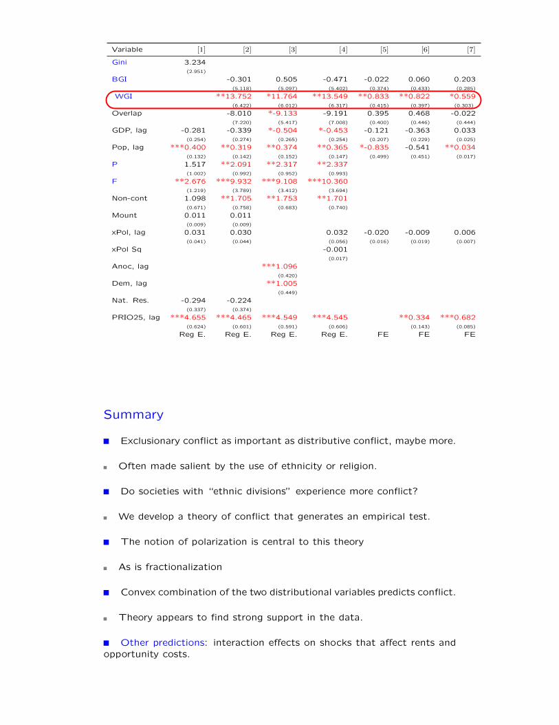
Variable [1] [2] [3] [4] [5] [6] [7]

Gini 3.234(2.951)

BGI -0.301 0.505 -0.471 -0.022 0.060 0.203(5.118) (5.097) (5.402) (0.374) (0.433) (0.285)

WGI **13.752 *11.764 **13.549 **0.833 **0.822 *0.559(6.422) (6.012) (6.317) (0.415) (0.397) (0.303)

Overlap -8.010 *-9.133 -9.191 0.395 0.468 -0.022(7.220) (5.417) (7.008) (0.400) (0.446) (0.444)

GDP, lag -0.281 -0.339 *-0.504 *-0.453 -0.121 -0.363 0.033(0.254) (0.274) (0.265) (0.254) (0.207) (0.229) (0.025)

Pop, lag ***0.400 **0.319 **0.374 **0.365 *-0.835 -0.541 **0.034(0.132) (0.142) (0.152) (0.147) (0.499) (0.451) (0.017)

P 1.517 **2.091 **2.317 **2.337(1.002) (0.992) (0.952) (0.993)

F **2.676 ***9.932 ***9.108 ***10.360(1.219) (3.789) (3.412) (3.694)

Non-cont 1.098 **1.705 **1.753 **1.701(0.671) (0.758) (0.683) (0.740)

Mount 0.011 0.011(0.009) (0.009)

xPol, lag 0.031 0.030 0.032 -0.020 -0.009 0.006(0.041) (0.044) (0.056) (0.016) (0.019) (0.007)

xPol Sq -0.001(0.017)

Anoc, lag ***1.096(0.420)

Dem, lag **1.005(0.449)

Nat. Res. -0.294 -0.224(0.337) (0.374)

PRIO25, lag ***4.655 ***4.465 ***4.549 ***4.545 **0.334 ***0.682(0.624) (0.601) (0.591) (0.606) (0.143) (0.085)

Reg E. Reg E. Reg E. Reg E. FE FE FE

0-62

Summary

Exclusionary conflict as important as distributive conflict, maybe more.

Often made salient by the use of ethnicity or religion.

Do societies with “ethnic divisions” experience more conflict?

We develop a theory of conflict that generates an empirical test.

The notion of polarization is central to this theory

As is fractionalization

Convex combination of the two distributional variables predicts conflict.

Theory appears to find strong support in the data.

Other predictions: interaction e↵ects on shocks that a↵ect rents andopportunity costs.

0-63