Slides 9

Debraj Ray

Columbia, Fall 2013

Credit Markets

Collateral

Adverse selection

Moral hazard

Enforcement

0-0

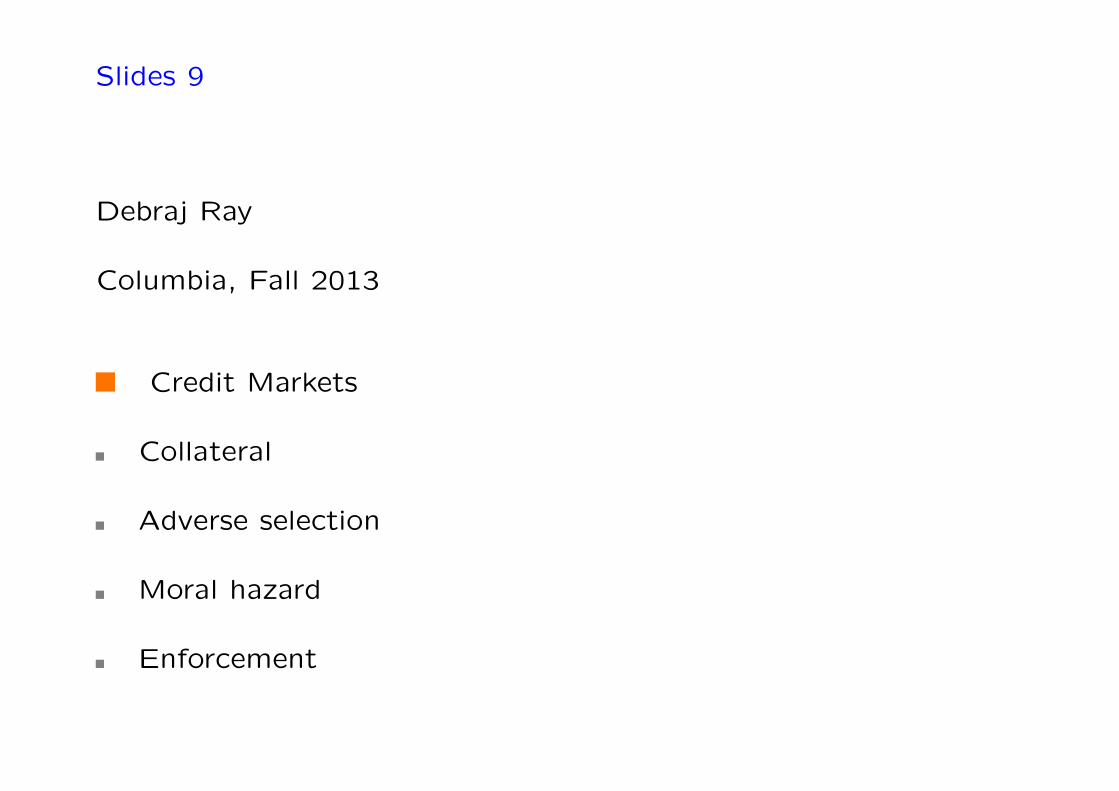
Credit Markets

Formal sector:

State or commercial banks.

Require collateral, business plan

Usually lend to registered firms or small businesses

Usually charge the lowest rates of interest

Often give directed credit to “priority sectors”:

(exports, agriculture, small business)

0-1

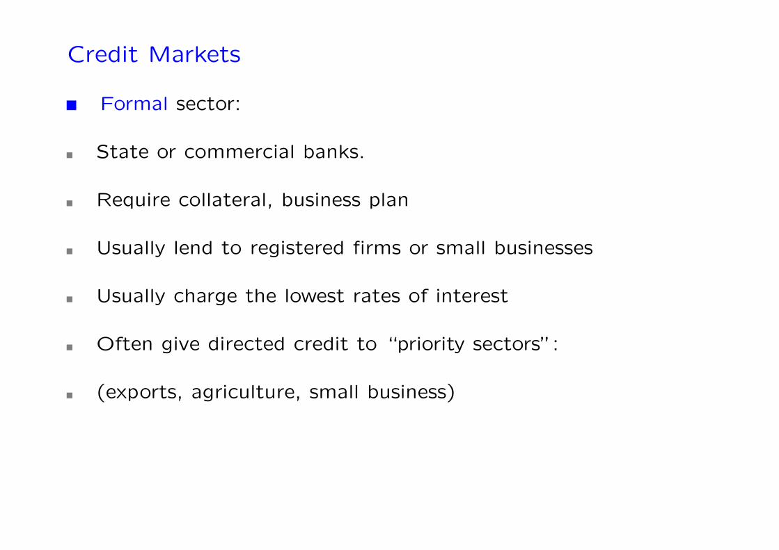
Informal sector:

Moneylender, trader, landlord, shopkeeper . . .

Better information

Better enforcement capabilities (multi-market)

Specific abilities to take certain types of collateral

Can price out distortions via multi-market contact

Quasi-formal organizations:

Grameen Bank, microfinance NGOs

Sometimes use group liability to avoid default

Rigid repayment schedules

Working capital rather than fixed capital loans

0-2

Some Stylized Facts

What follows is all interrelated, of course.

Collateral matters: the richer get better deals.

Relationship between collateral and interest rates

The form of collateral matters too:

Landlords lend to tenants and small-holders.

Traders lend to farmers producing the same crop they trade.

Occupation-based lending: Bangladeshi immigrants.

0-3

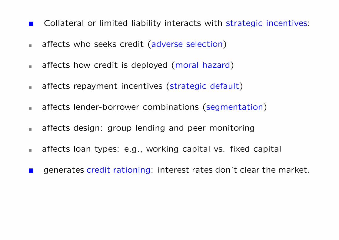
Collateral or limited liability interacts with strategic incentives:

affects who seeks credit (adverse selection)

affects how credit is deployed (moral hazard)

affects repayment incentives (strategic default)

affects lender-borrower combinations (segmentation)

affects design: group lending and peer monitoring

affects loan types: e.g., working capital vs. fixed capital

generates credit rationing: interest rates don’t clear the market.

0-4

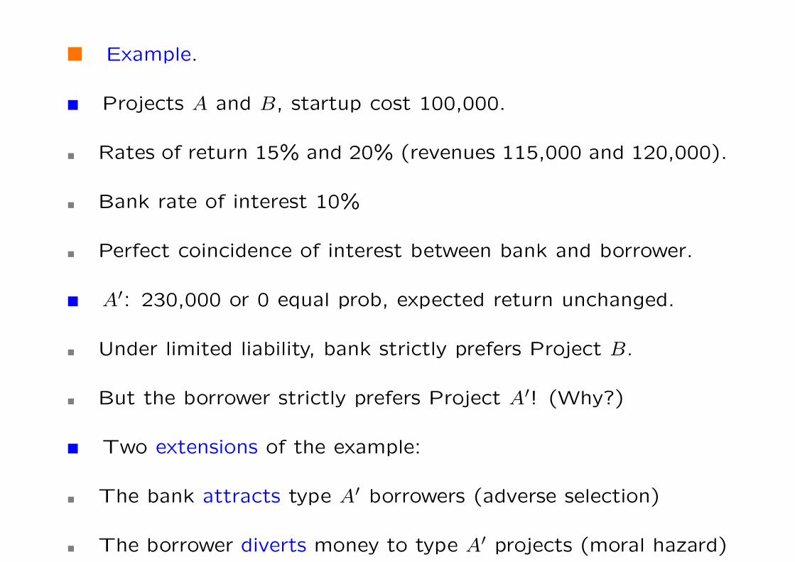
Example.

Projects A and B, startup cost 100,000.

Rates of return 15% and 20% (revenues 115,000 and 120,000).

Bank rate of interest 10%

Perfect coincidence of interest between bank and borrower.

A′: 230,000 or 0 equal prob, expected return unchanged.

Under limited liability, bank strictly prefers Project B.

But the borrower strictly prefers Project A′! (Why?)

Two extensions of the example:

The bank attracts type A′ borrowers (adverse selection)

The borrower diverts money to type A′ projects (moral hazard)

0-5

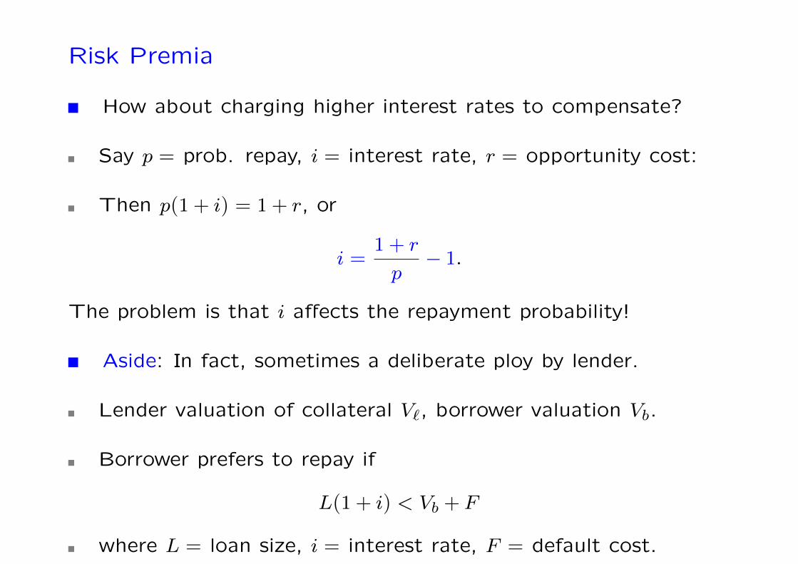
Risk Premia

How about charging higher interest rates to compensate?

Say p = prob. repay, i = interest rate, r = opportunity cost:

Then p(1+ i) = 1+ r, or

i =1+ r

p− 1.

The problem is that i affects the repayment probability!

Aside: In fact, sometimes a deliberate ploy by lender.

Lender valuation of collateral V`, borrower valuation Vb.

Borrower prefers to repay if

L(1+ i) < Vb + F

where L = loan size, i = interest rate, F = default cost.

0-6

Aside, contd.

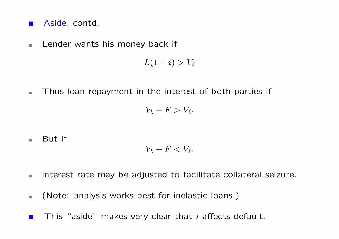
Lender wants his money back if

L(1+ i) > V`

Thus loan repayment in the interest of both parties if

Vb + F > V`.

But ifVb + F < V`.

interest rate may be adjusted to facilitate collateral seizure.

(Note: analysis works best for inelastic loans.)

This “aside” makes very clear that i affects default.

0-7

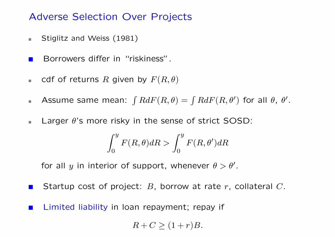
Adverse Selection Over Projects

Stiglitz and Weiss (1981)

Borrowers differ in “riskiness”.

cdf of returns R given by F (R, θ)

Assume same mean:∫RdF (R, θ) =

∫RdF (R, θ′) for all θ, θ′.

Larger θ’s more risky in the sense of strict SOSD:∫ y

0F (R, θ)dR >

∫ y

0F (R, θ′)dR

for all y in interior of support, whenever θ > θ′.

Startup cost of project: B, borrow at rate r, collateral C.

Limited liability in loan repayment; repay if

R+C ≥ (1+ r)B.

0-8

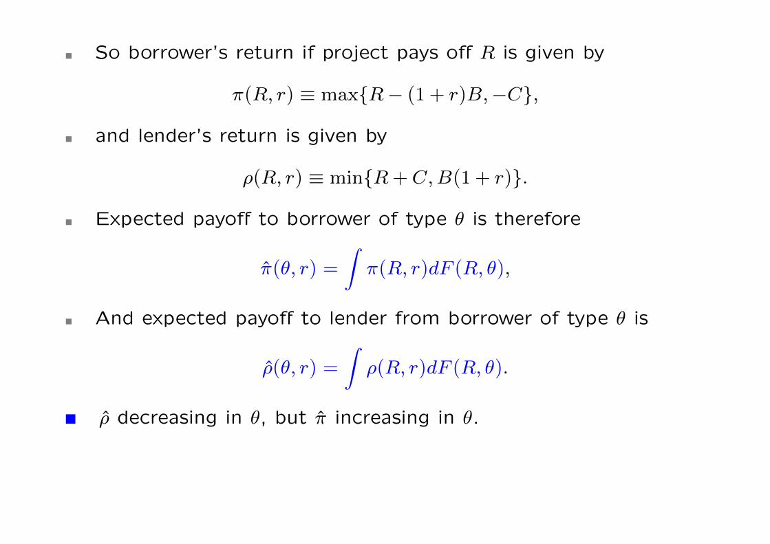
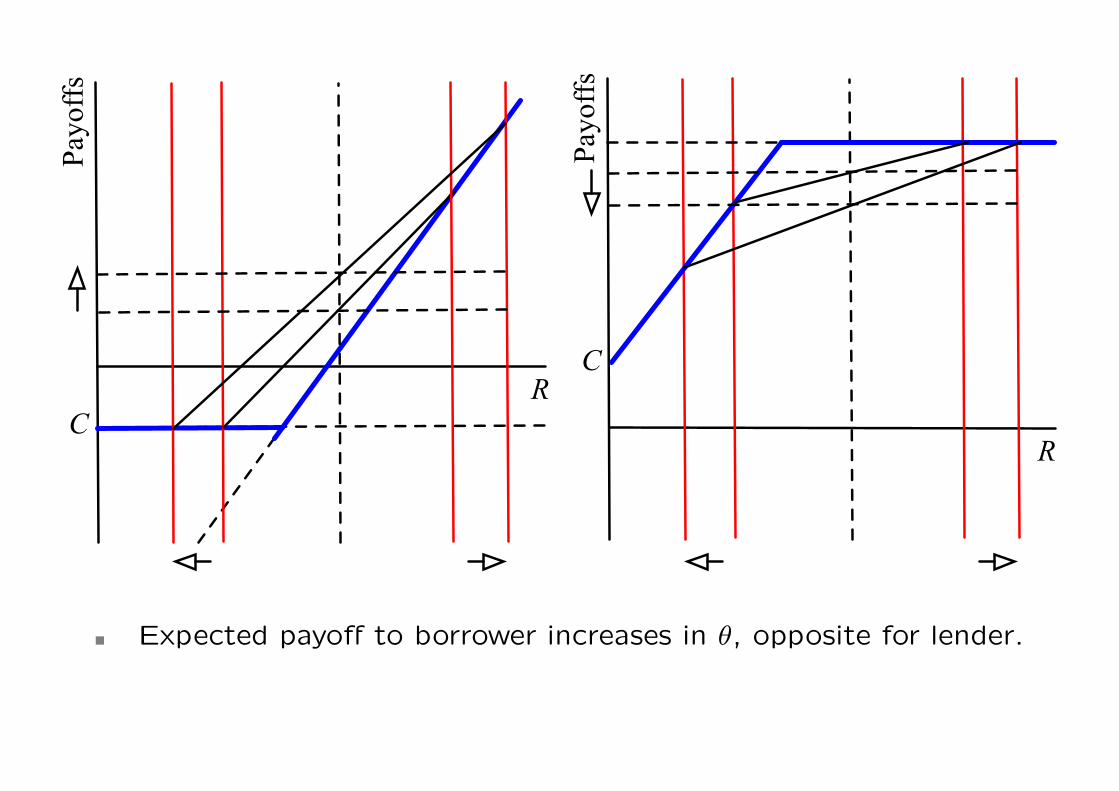
So borrower’s return if project pays off R is given by

π(R, r) ≡ max{R− (1+ r)B,−C},

and lender’s return is given by

ρ(R, r) ≡ min{R+C,B(1+ r)}.

Expected payoff to borrower of type θ is therefore

π(θ, r) =

∫π(R, r)dF (R, θ),

And expected payoff to lender from borrower of type θ is

ρ(θ, r) =

∫ρ(R, r)dF (R, θ).

ρ decreasing in θ, but π increasing in θ.

0-9

R

Payoffs

CR

Payoffs

C

Expected payoff to borrower increases in θ, opposite for lender.

0-10

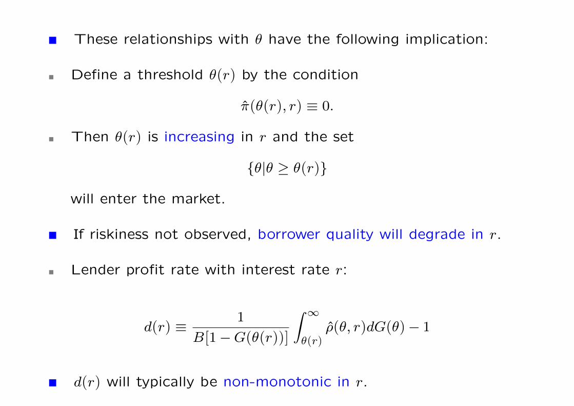
These relationships with θ have the following implication:

Define a threshold θ(r) by the condition

π(θ(r), r) ≡ 0.

Then θ(r) is increasing in r and the set

{θ|θ ≥ θ(r)}

will enter the market.

If riskiness not observed, borrower quality will degrade in r.

Lender profit rate with interest rate r:

d(r) ≡1

B[1−G(θ(r))]

∫ ∞θ(r)

ρ(θ, r)dG(θ)− 1

d(r) will typically be non-monotonic in r.

0-11

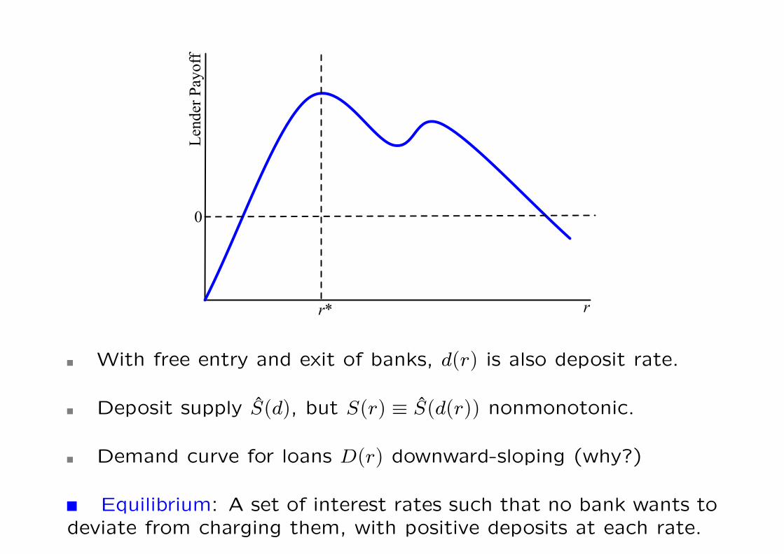
r

Lend

er P

ayof

f0

r*

With free entry and exit of banks, d(r) is also deposit rate.

Deposit supply S(d), but S(r) ≡ S(d(r)) nonmonotonic.

Demand curve for loans D(r) downward-sloping (why?)

Equilibrium: A set of interest rates such that no bank wants todeviate from charging them, with positive deposits at each rate.

0-12

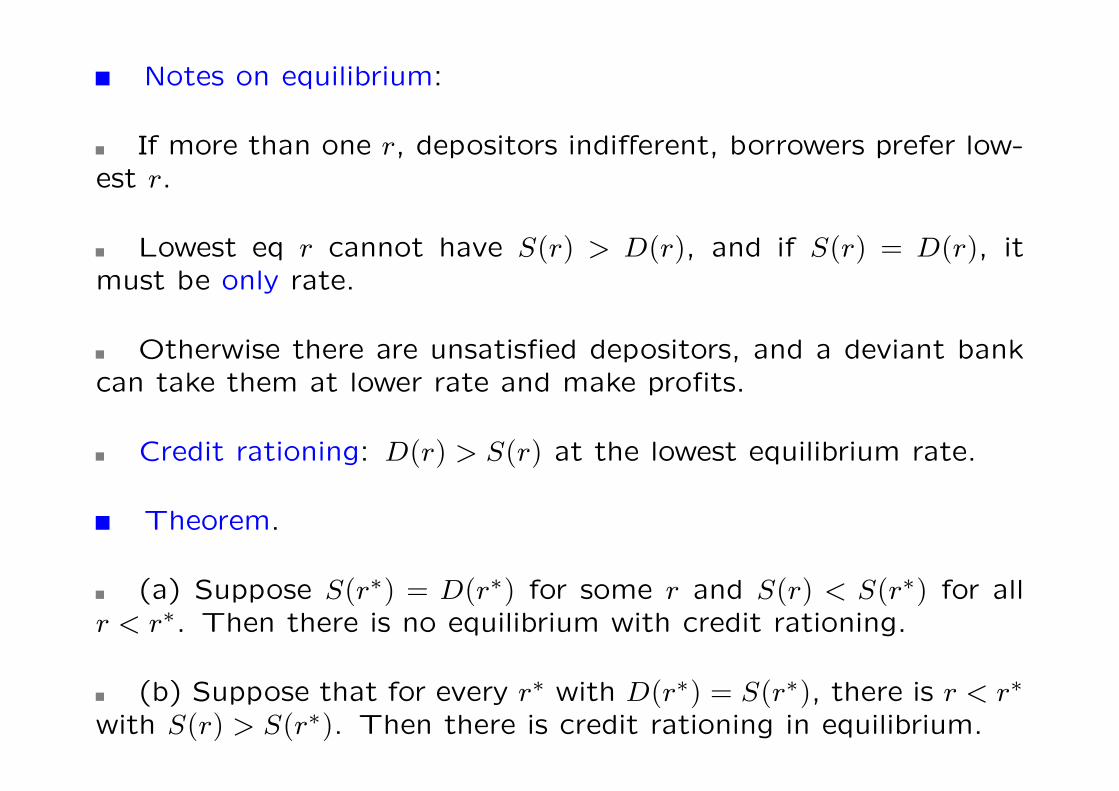
Notes on equilibrium:

If more than one r, depositors indifferent, borrowers prefer low-est r.

Lowest eq r cannot have S(r) > D(r), and if S(r) = D(r), itmust be only rate.

Otherwise there are unsatisfied depositors, and a deviant bankcan take them at lower rate and make profits.

Credit rationing: D(r) > S(r) at the lowest equilibrium rate.

Theorem.

(a) Suppose S(r∗) = D(r∗) for some r and S(r) < S(r∗) for allr < r∗. Then there is no equilibrium with credit rationing.

(b) Suppose that for every r∗ with D(r∗) = S(r∗), there is r < r∗

with S(r) > S(r∗). Then there is credit rationing in equilibrium.

0-13

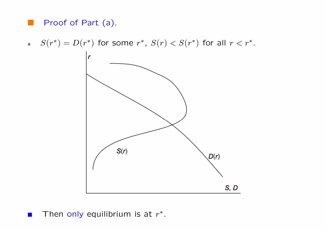
Proof of Part (a).

S(r∗) = D(r∗) for some r∗, S(r) < S(r∗) for all r < r∗.

Then only equilibrium is at r∗.

0-14

If any eq r below r∗, then every other eq r′ above r∗ to maintaindepositor indifference.

Deviant bank: offers r∗, and some d ∈ (d(r), d(r∗)), takes all therationed borrowers from r, makes positive profit.

If every eq r no less than r∗, let r1 be lowest of them.

By earlier note, D(r1) ≥ S(r1) and if r1 = r∗, then unique.

So suppose that r1 > r∗. Then S(r1) ≤ D(r1) < D(r∗) = S(r∗).

So S(r) > S(r∗) and consequently, d(r) > d(r∗).

Deviant bank charges r = r∗, offers d′ ∈ (d(r∗), d(r)), gets alldepositors and borrowers, makes positive profits.

0-15

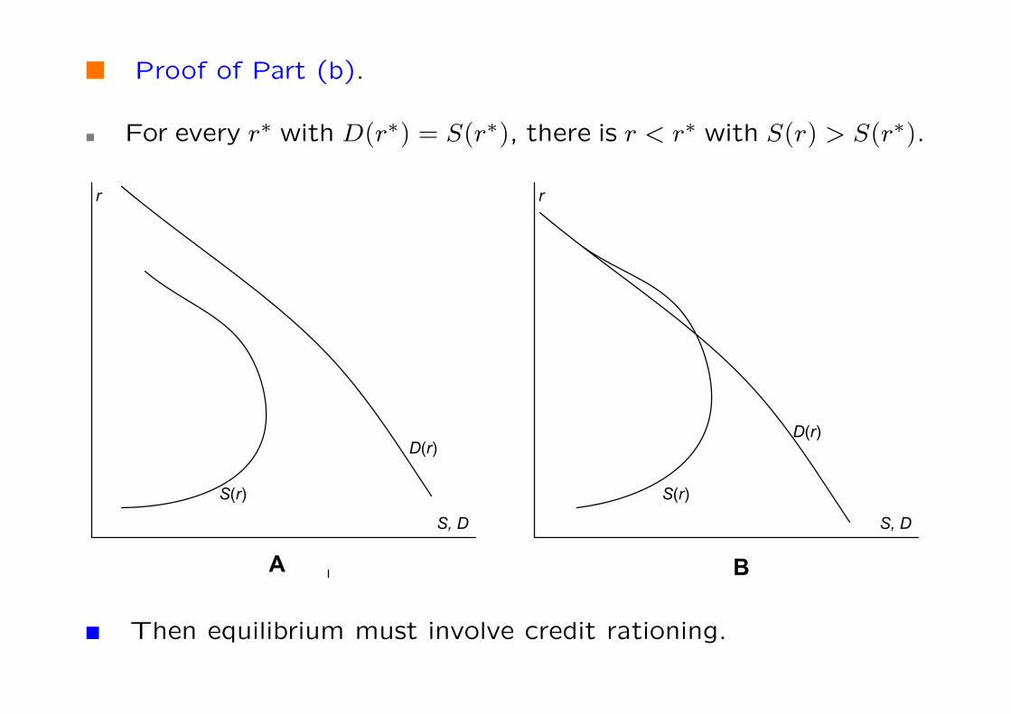
Proof of Part (b).

For every r∗ with D(r∗) = S(r∗), there is r < r∗ with S(r) > S(r∗).

D r

S r

r

S, D

D r

S r

r

S, D

D rS r

r

S, D

Then equilibrium must involve credit rationing.

0-16

Suppose not, then single-r equilibrium at r∗ with S(r∗) = D(r∗).

We know that S(r) > S(r∗) for some r < r∗.

So d(r) > d(r∗).

Deviant bank offers r and d ∈ (d(r∗), d(r)), makes profits.

Remains to demonstrate equilibrium with credit rationing.

Let r∗∗ be the smallest maximizer of d(r).

If D(r∗∗) > S(r∗∗), then done: set r = r∗∗.

Otherwise, D(r∗∗) < S(r∗∗) (equality violates part (b)).

In this case, let r∗ be Walrasian equilibrium below it.

By assumption, there is r1 < r∗ with S(r1) > S(r∗).

Choose r1 as first conditional maximizer of S(r) below r∗.

0-17

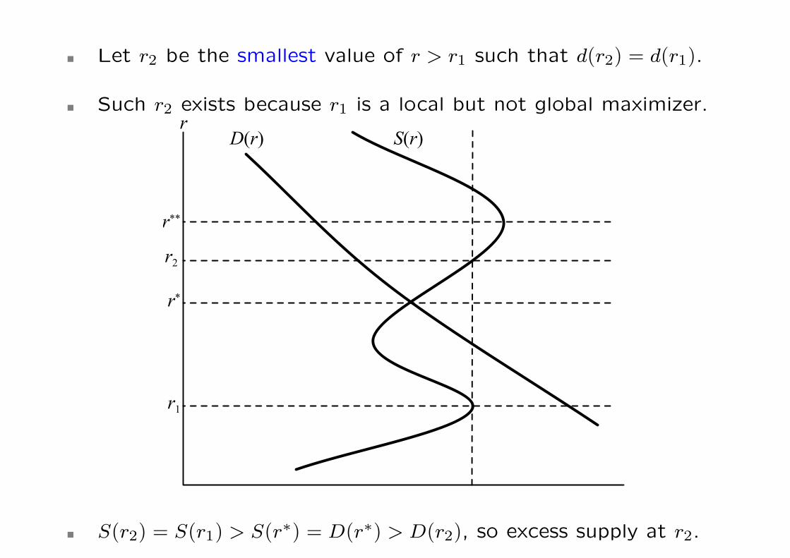
Let r2 be the smallest value of r > r1 such that d(r2) = d(r1).

Such r2 exists because r1 is a local but not global maximizer.r

r**

r*

D(r) S(r)

r1

r2

S(r2) = S(r1) > S(r∗) = D(r∗) > D(r2), so excess supply at r2.

0-18

Complete the proof:

Take the equilibrium set to be {r1, r2}.

If all funds go to r1, excess demand, if all to r2 excess supply.

Using depositor indifference, find allocation to exactly matchdemand and supply.

Check that this is an equilibrium with credit rationing.

(No one can deviate, not even to r∗∗.)

0-19

Moral Hazard in Project Choice

Now we allow borrowers to choose from different projects.

Projects indexed by θ.

Return Q(θ) with prob p(θ), 0 with prob 1− p(θ).

Arrange such that Q(θ) increasing, wlog p(θ) decreasing.

Each project requires the same loan size of B.

Borrower with collateral C, facing r, chooses θ to max

p(θ) [Q(θ)−B(1+ r)]− [1− p(θ)]C,

where Q(θ) exceeds B(1+ r), otherwise no borrowing.

Determines riskiness θ(C, r) as a function of C and r.

0-20

Proposition:

θ(C, r) is decreasing in C and increasing in r.

Collateral induces safety; interest rates induce risk.

Proof. Define Z = B(1+ r)−C. Borrower picks θ to maximize

p(θ)[Q(θ)−Z].

Let Z1 > Z2. Let θ1 and θ2 be the two maxima (assume unique):

Then p(θ1)[Q(θ1)−Z1] > p(θ2)[Q(θ2)−Z1],

while p(θ2)[Q(θ2)−Z2] > p(θ1)[Q(θ1)−Z2].

Adding these two inequalities, we can conclude that

[p(θ1)− p(θ2)] (Z1 −Z2) < 0.

Therefore p(θ) is increasing in Z.

0-21

Credit rationing:

Entirely possible that for low values of C,

maxrp(θ(C, r))(1+ r) < 1+ r

where r is opportunity cost of funds.

Collateral and interest:

Under competitive lending,

p(θ(C, r))B(1+ r) + [1− p(θ(C, r))]C = B[1+ r].

LHS as function of r. Nonmonotone, with end-point conditions.

0-22

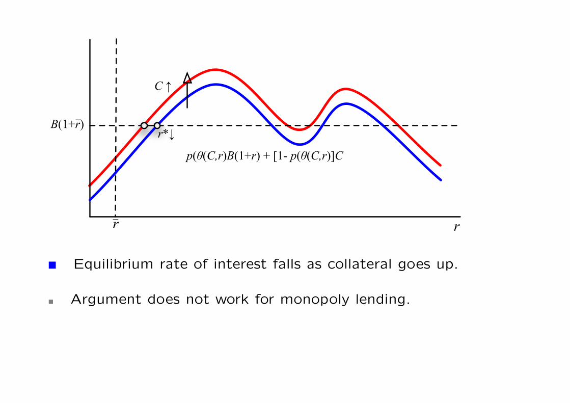
B(1+r)_

p(θ(C,r)B(1+r) + [1- p(θ(C,r)]C

rr_

C ↑

r*↓

Equilibrium rate of interest falls as collateral goes up.

Argument does not work for monopoly lending.

0-23

Moral Hazard and the Debt Overhang

Costly effort can influence success probabilities.

Project requires startup of B.

Output is either Q (good) or 0 (bad).

Probability of good output is p(e), where e = agent effort.

If agent is self-financed, choose e to maximize

p(e)Q− e−L.

Assume unique choice e∗; described by the first-order condition

p′(e∗) =1

Q

This is the efficient, or first-best level of effort.

0-24

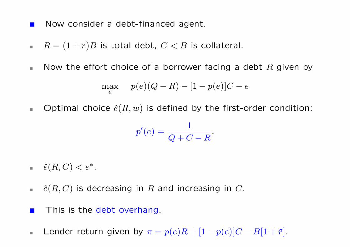
Now consider a debt-financed agent.

R = (1+ r)B is total debt, C < B is collateral.

Now the effort choice of a borrower facing a debt R given by

maxe

p(e)(Q−R)− [1− p(e)]C − e

Optimal choice e(R,w) is defined by the first-order condition:

p′(e) =1

Q+C −R.

e(R,C) < e∗.

e(R,C) is decreasing in R and increasing in C.

This is the debt overhang.

Lender return given by π = p(e)R+ [1− p(e)]C −B[1+ r].

0-25

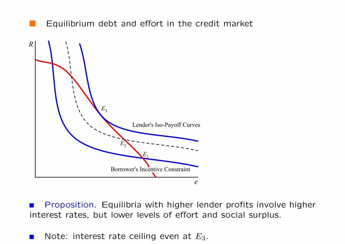
Equilibrium debt and effort in the credit market

e

R

Lender's Iso-Payoff Curves

Borrower's Incentive Constraint

E1

E2

E3

Proposition. Equilibria with higher lender profits involve higherinterest rates, but lower levels of effort and social surplus.

Note: interest rate ceiling even at E3.

0-26

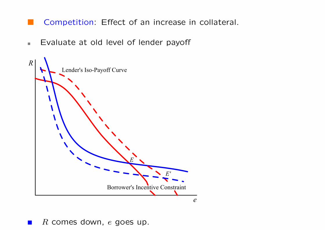
Competition: Effect of an increase in collateral.

Evaluate at old level of lender payoff

e

RLender's Iso-Payoff Curve

Borrower's Incentive Constraint

E

E'

R comes down, e goes up.

0-27

Monopoly: Effect of an increase in collateral.

Lender maximizes in each case, subject to incentive constraint.

e

R

Lender's Iso-Payoff Curve

Borrower's Incentive Constraint

E

E'

(Generally) R and e will both go up.

0-28

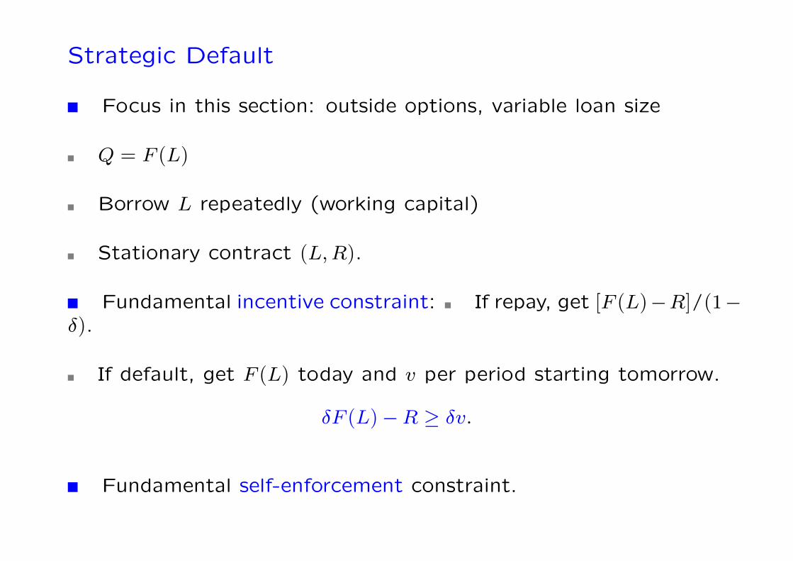
Strategic Default

Focus in this section: outside options, variable loan size

Q = F (L)

Borrow L repeatedly (working capital)

Stationary contract (L,R).

Fundamental incentive constraint: If repay, get [F (L)−R]/(1−δ).

If default, get F (L) today and v per period starting tomorrow.

δF (L)−R ≥ δv.

Fundamental self-enforcement constraint.

0-29

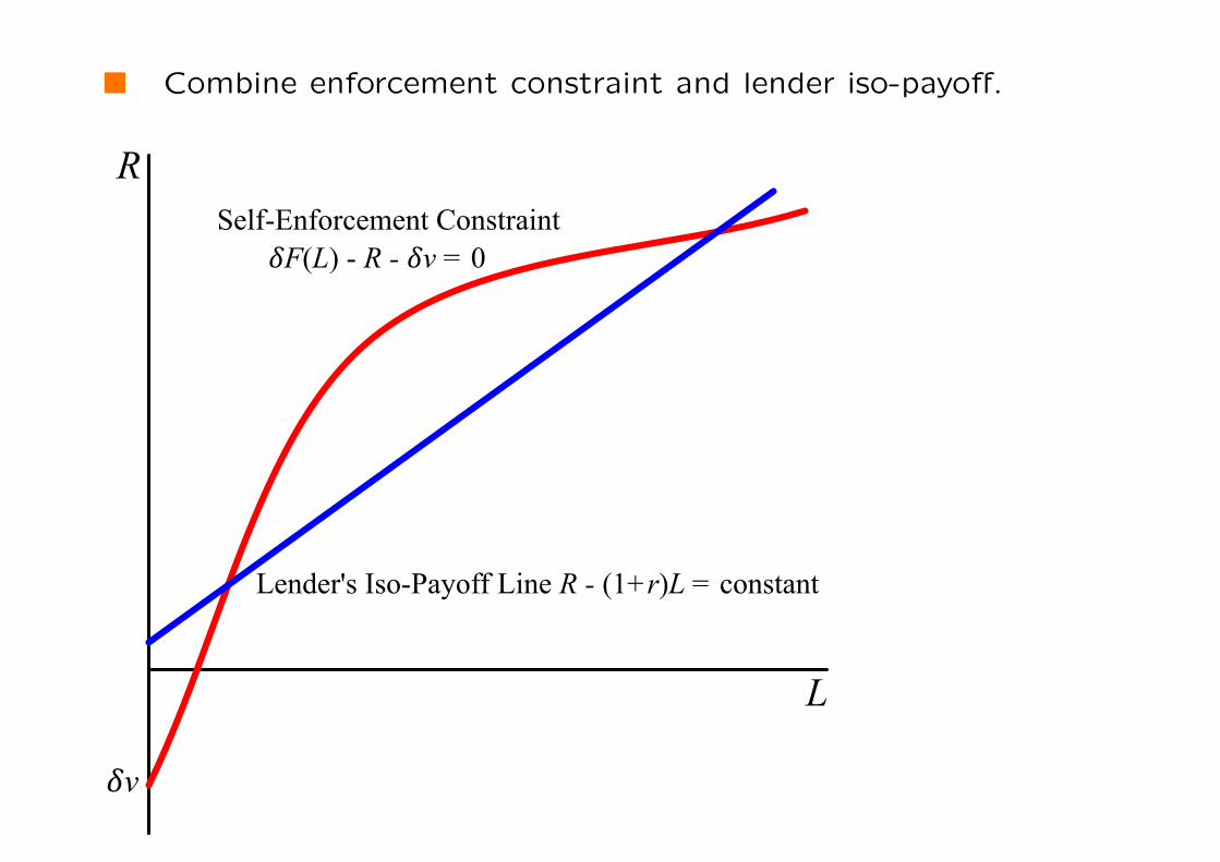
Combine enforcement constraint and lender iso-payoff.

L

R

Lender's Iso-Payoff Line R - (1+r)L = constant

Self-Enforcement Constraint

!v

!F(L) - R - !v = 0

0-30

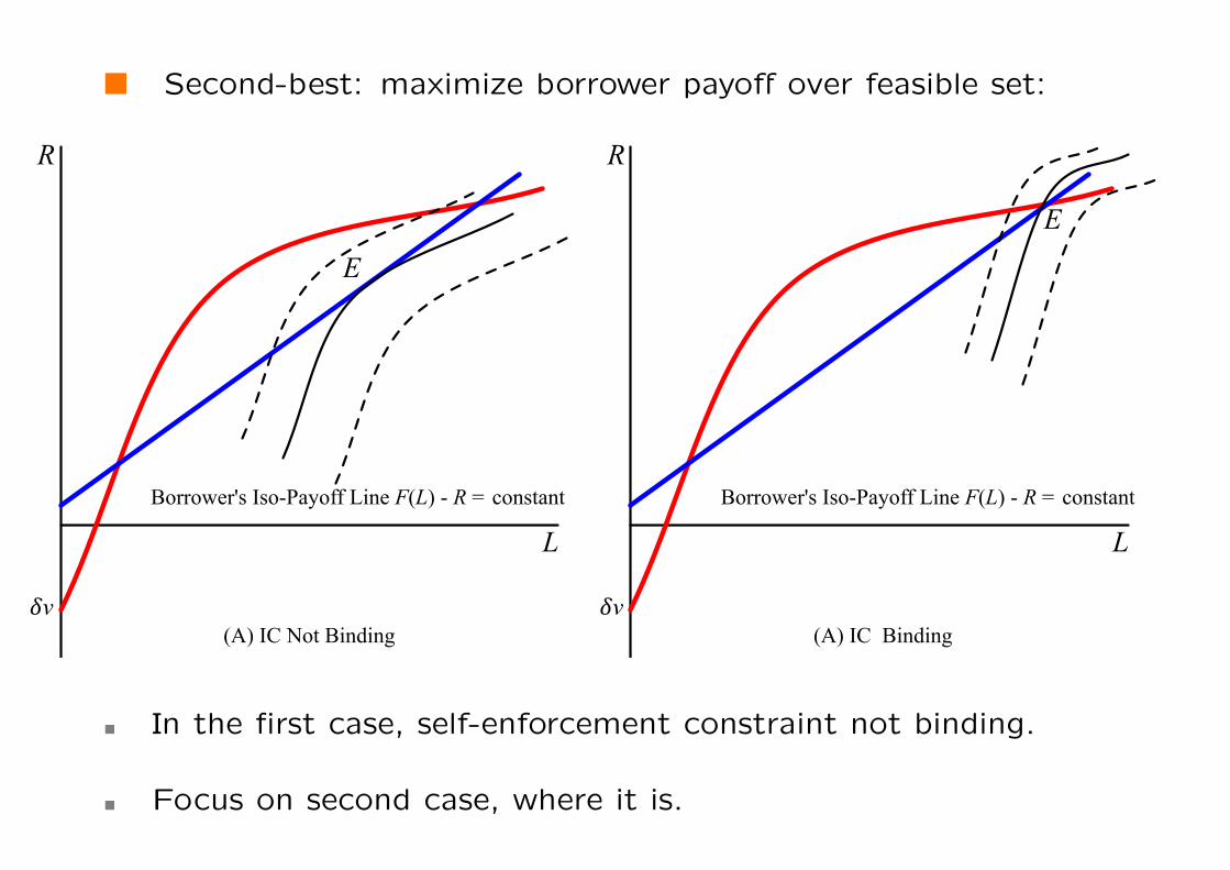
Second-best: maximize borrower payoff over feasible set:

L

R

!v

Borrower's Iso-Payoff Line F(L) - R = constant

L

R

!v

Borrower's Iso-Payoff Line F(L) - R = constant

(A) IC Not Binding (A) IC Binding

E

E

In the first case, self-enforcement constraint not binding.

Focus on second case, where it is.

0-31

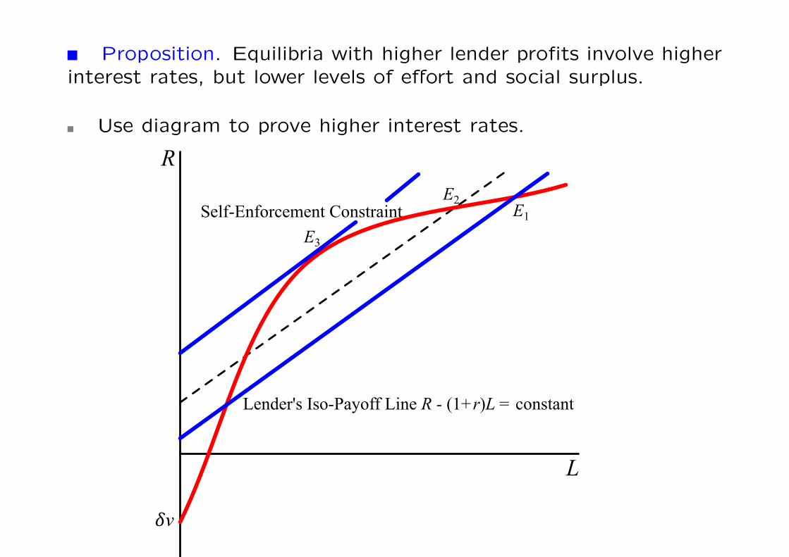
Proposition. Equilibria with higher lender profits involve higherinterest rates, but lower levels of effort and social surplus.

Use diagram to prove higher interest rates.

L

R

Lender's Iso-Payoff Line R - (1+r)L = constant

Self-Enforcement Constraint E1

E2

E3

!v

0-32

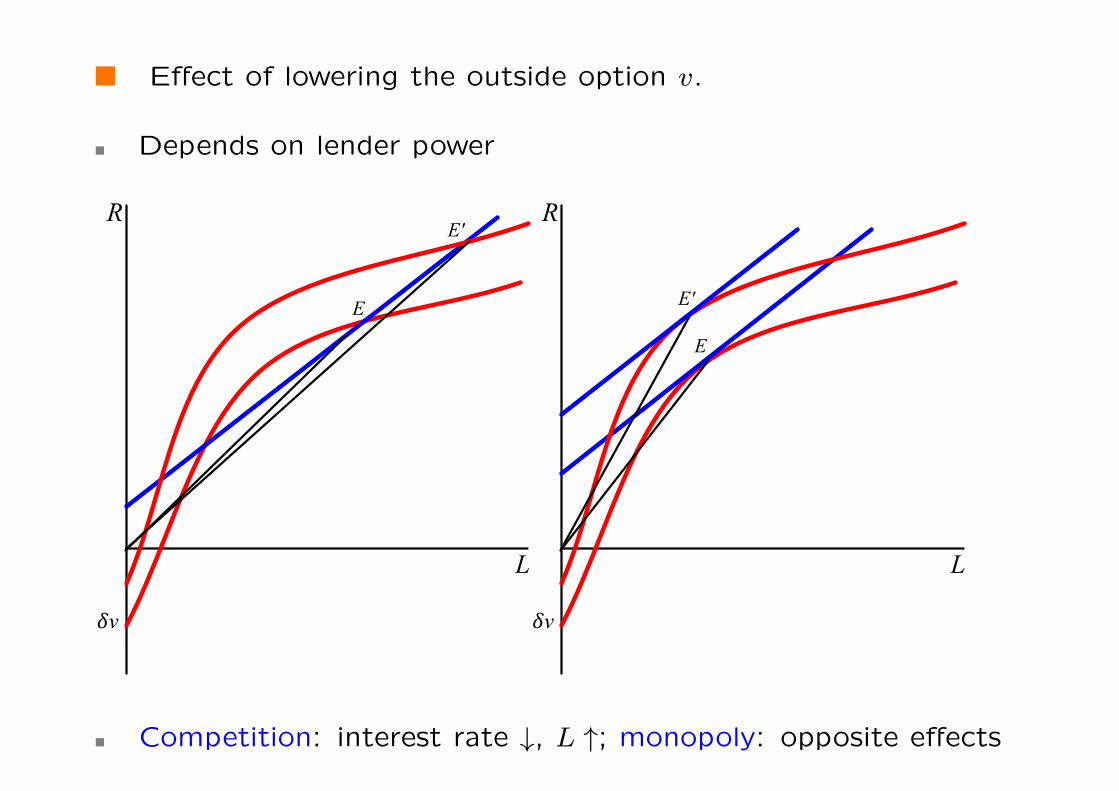
Effect of lowering the outside option v.

Depends on lender power

L

R

E

!v

E'

L

R

E

!v

E'

Competition: interest rate ↓, L ↑; monopoly: opposite effects

0-33

Information and Equilibrium in Credit Markets

Where does the outside option v come from?

Expected value conditional on termination of relationship.

The reason matters, how much is known to others.

Thus, v may also incorporate punishment following default.

Say competitive lending market. Recall, borrrowers maximize

F (L)− (1+ r)L

subject to the incentive constraint

F (L)−1+ r

δL ≥ v.

Let w(v) be the maximized value.

0-34

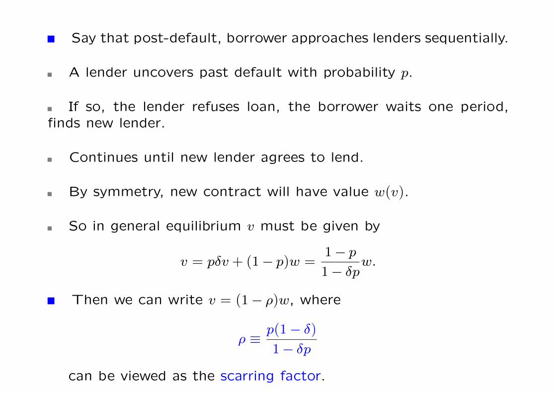
Say that post-default, borrower approaches lenders sequentially.

A lender uncovers past default with probability p.

If so, the lender refuses loan, the borrower waits one period,finds new lender.

Continues until new lender agrees to lend.

By symmetry, new contract will have value w(v).

So in general equilibrium v must be given by

v = pδv + (1− p)w =1− p1− δp

w.

Then we can write v = (1− ρ)w, where

ρ ≡p(1− δ)1− δp

can be viewed as the scarring factor.

0-35

Notes on the scarring factor:

If p is close to one, so is the scarring factor ρ.

On the other hand, ρ→ 0 as δ converges to one.

(But wait for a final verdict on the net effect of patience.)

Theorem. Define

ρ∗ ≡(1+ r)(1− δ)L/δF (L)− (1+ r)L

∈ (0, 1),

where L is the maximizer of F (L)− 1+rδL.

Then a competitive equilibrium exists if and only if ρ ≥ ρ∗.

Implications for theories of social capital.

Information and development.

0-36

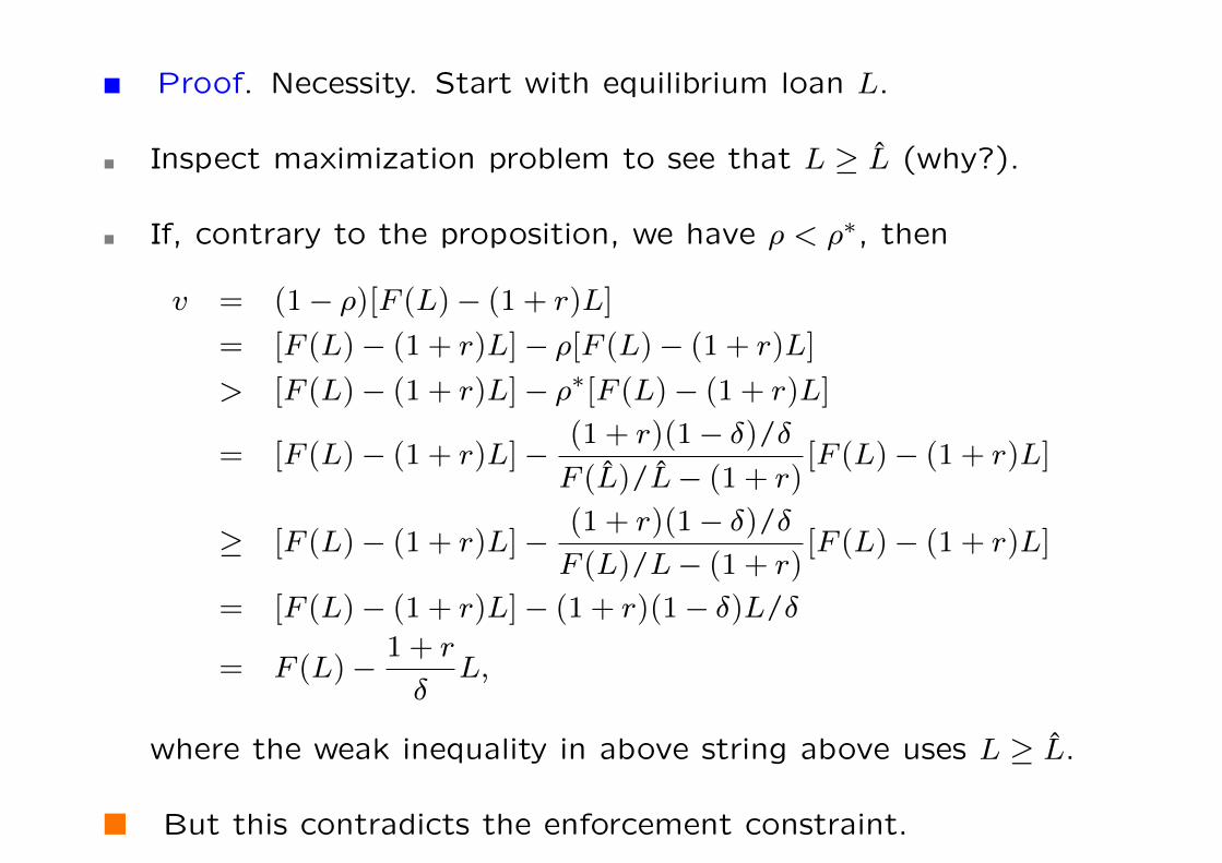
Proof. Necessity. Start with equilibrium loan L.

Inspect maximization problem to see that L ≥ L (why?).

If, contrary to the proposition, we have ρ < ρ∗, then

v = (1− ρ)[F (L)− (1+ r)L]

= [F (L)− (1+ r)L]− ρ[F (L)− (1+ r)L]

> [F (L)− (1+ r)L]− ρ∗[F (L)− (1+ r)L]

= [F (L)− (1+ r)L]−(1+ r)(1− δ)/δF (L)/L− (1+ r)

[F (L)− (1+ r)L]

≥ [F (L)− (1+ r)L]−(1+ r)(1− δ)/δF (L)/L− (1+ r)

[F (L)− (1+ r)L]

= [F (L)− (1+ r)L]− (1+ r)(1− δ)L/δ

= F (L)−1+ r

δL,

where the weak inequality in above string above uses L ≥ L.

But this contradicts the enforcement constraint.

0-37

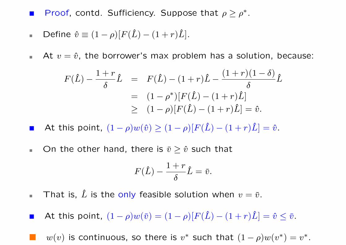
Proof, contd. Sufficiency. Suppose that ρ ≥ ρ∗.

Define v ≡ (1− ρ)[F (L)− (1+ r)L].

At v = v, the borrower’s max problem has a solution, because:

F (L)−1+ r

δL = F (L)− (1+ r)L−

(1+ r)(1− δ)δ

L

= (1− ρ∗)[F (L)− (1+ r)L]

≥ (1− ρ)[F (L)− (1+ r)L] = v.

At this point, (1− ρ)w(v) ≥ (1− ρ)[F (L)− (1+ r)L] = v.

On the other hand, there is v ≥ v such that

F (L)−1+ r

δL = v.

That is, L is the only feasible solution when v = v.

At this point, (1− ρ)w(v) = (1− ρ)[F (L)− (1+ r)L] = v ≤ v.

w(v) is continuous, so there is v∗ such that (1− ρ)w(v∗) = v∗.

0-38

Interlinked Contracts

Market segmentation:

Landlord lends to tenant, the trader to farmers, etc.

Reasons for interlinkage:

Assurance. Fixed costs need to be covered in trading. So “tieup” farmers by giving them loans in exchange for the promise ofoutput sales to him.

Enforcement. Using double-threats; e.g., remove tenancy con-tract as well as future loan contracts if default on the loan contract.

Nonmarketable Collateral. In interlinked relationships, easier toaccept non marketable collateral. (Note” doesn’t explain if thecontract per se is interlinked.)

Removal of Distortions. Multi-dimensional pricing.

0-39

Summary

Fundamental to credit markets is the problem of limited liability.

Limited liability affected by the ability to post collateral.

This has three channels of influence:

Via adverse selection: project mix becomes excessively risky

Via moral hazard: borrowers put in too little effort to repay

Via strategic default: borrowers take outside options

In all cases, lender power is correlated with inefficient outcomes.

Lender power more likely when there is segmentation.

0-40