Embed Size (px)
Citation preview

Unemployment and Capital Misallocation∗
Job Market Paper
Feng Dong†
Washington University in St. Louis
download the latest version
November 18, 2013
Abstract
The recent recession was associated not only with a marked disruption in the credit
market, but also with an outward shift in the Beveridge curve. Motivated by the joint de-
terioration of the credit and labor markets, we develop a tractable dynamic model with
heterogeneous entrepreneurs, and with credit and labor-search frictions. In this framework,
the misallocation of capital across firms has an adverse effect on search efficiency. We then
quantify the unemployment effect of this misallocation. On the one hand, the credit crunch
is a key driving force behind the recent outward shift in the Beveridge curve. On the other
hand, credit imperfections and labor search frictions contribute 46% and 54%, respectively,
to unemployment over all business cycles between 1951 and 2011.
Key Words: Credit Crunch, Capital/Labor Misallocation, Beveridge Curve, Jobless Recovery.
∗I am deeply indebted to Steve Williamson, Costas Azariadis, Yongseok Shin and Yi Wen for their constant advice and
support. I also benefited from comments by Gaetano Antinolfi, Saki Bigio, Francisco Buera, Wei Cui, Hugo Hopenhayn,
Yang Jiao, Ricardo Lagos, Rody Manuelli, Ellen McGrattan, Ben Moll, Min Ouyang, Ali Ozdagli, Vincenzo Quadrini, B.
Ravikumar, Diego Restuccia, Juan M. Sánchez, Pengfei Wang, Ping Wang, Wei Wang, Pierre-Olivier Weill, David Wiczer,
Tao Zha, Xiaodong Zhu, and participants in the Midwest Macro Meeting at UIUC, North American Summer Meeting
of Econometric Society at USC, Tsinghua Workshop in Macroeconomics, the Summer Workshop on Money, Banking,
Payments and Finance by Chicago Fed, Econ Con at Columbia University, seminars at St. Louis Fed and Washington
University, and the Midwest Macro Meeting at Minnesota. All errors are mine.†Email: [email protected]. Website: fengdongecon.weebly.com.
1

1 Introduction
The recent financial crisis was accompanied by a marked increase in unemployment and a serious dis-
ruption in credit markets. One the one hand, as the left panel of Figure (1.1) shows, not only did the
unemployment rate increase significantly over time, but the Beveridge curve also shifted outward be-
ginning in the last quarter of 2008, when Lehmann Brothers collapsed. On the other hand, the ratio of
external funding to non-financial assets, a key measure used in the literature to characterize the func-
tioning of the credit market, shrank significantly, as demonstrated in the right panel of Figure (1.1).1
Motivated by the joint deterioration of the labor and credit markets in the recent recession, this paper
models and quantifies the unemployment effect of capital misallocation due to credit imperfections.
By developing a tractable dynamic model with heterogeneous entrepreneurs, and with credit and labor
frictions, we propose a novel channel through which capital misallocation lowers aggregate matching
efficiency in the labor market. Our quantitative analysis implies that the credit crunch caused by the
recent financial crisis served as the key driving force behind the outward shift in the Beveridge curve.
Moreover, credit imperfections and labor search frictions are shown to contribute 46% and 54%, respec-
tively, to unemployment over all business cycles between 1951 and 2011.
0.04 0.06 0.08 0.10.015
0.02
0.025
0.03
0.035
0.04
0.045
Unemployment Rate
Job
Ope
ning
Rat
e
Date
Ext
erna
l Fun
ding
ove
r N
on-F
in A
sset
s
2006 2008 2010 20120.65
0.7
0.75
0.8
0.85
2008Q4
2000Q4
2008Q4
2011Q4
2008Q1
Figure 1.1: Left Panel: Beveridge Curve, Job Openings and Labor Turnover Survey (JOLTS); Right Panel:External Funding over Non-Financial Assets of Non-Financial Business, Flow of Funds Accounts
1The measure is considered in Buera and Moll (2013) and Buera, Fattal-Jaef and Shin (2013). Both non-financial cor-
porate and non-financial non-corporate business in the Flow of Funds Accounts are considered. Details are documented in
Appendix A.
2

We employ two layers of frictions to model the relationship between credit and labor markets. On
the one hand, we introduce credit frictions by using a collateral constraint, which is a powerful tool
to characterize credit crunches. On the other hand, we use competitive search to model equilibrium
unemployment. Recent empirical findings by Davis, Faberman and Haltiwanger (2013) show that job-
filling rates vary significantly across firms. However, a direct implication of random search is that
job-filling rate is independent of firm’s heterogeneous characteristics. As will be shown in our model,
the prediction of competitive search is in line with the empirical regularity.
Entrepreneurs are heterogeneous in two dimensions, net worth and productivity. The former is
endogenous and the latter is an exogenous stochastic process. There are three sources of aggregate
shocks: i) a credit shock, i.e., the tightening of collateral constraints in the credit market; ii) a matching
shock, i.e., the decrease of matching efficiency in the labor market; and iii) an aggregate productivity
shock.2 When a credit crunch occurs, the collateral constraint tightens and more capital would have to
be used by relatively unproductive entrepreneurs. The key theoretical contribution of this paper is that
capital misallocation is shown to worsen labor misallocation, even though there is no disruption in the
labor market itself.3 Therefore credit imperfections contribute to endogenous matching efficiency in
equilibrium and thus to shifts in the Beveridge curve. In addition to analytically illustrating the effect
of capital misallocation on labor misallocation, we also show that equilibrium TFP is determined by the
interaction between credit and labor frictions.4
The key transmission mechanism proceeds as follows. Although workers are homogeneous, the
marginal value of being matched with labor increases with an entrepreneur’s productivity. Therefore,
entrepreneurs with heterogeneous productivity have an incentive to post different wage offers. We use
competitive search to implement this idea. Entrepreneurs with higher productivity tend to post higher
wage positions with more workers in a queue competing for those jobs. Thus the job-filling rate will be
higher for highly productive entrepreneurs. In equilibrium, wage dispersion for homogeneous workers
emerges with an endogenous set of segmented labor markets, as in standard competitive search models.
If there is a negative shock to the credit market, i.e., the collateral constraint tightens, then capi-
tal misallocation worsens, since the interest rate decreases and thus more capital is used by relatively
unproductive entrepreneurs. As argued above, since the job-filling rate in active sub-labor markets in-
creases with an entrepreneur’s productivity, the redistribution of capital from high-productivity to low-
productivity firms decreases the total number of matched workers. In addition to the direct effect im-
2The set of active sub-labor markets is endogenous. The details are shown in Section 3.3Since our model involves capital misallocation, it belongs to the recently burgeoning literature on misallocation, which
mainly includes Hsieh and Klenow (2009), Restuccia and Rogerson (2008), Bartelsman et al. (2012), and a recent discussion
by Hopenhayn (2013), among others. Moreover, there has been extensive discussion on capital misallocation due to financial
frictions, such as Buera, Kaboski and Shin (2011), Azariadis and Kaas (2012), Moll (2012), Wang and Wen (2012), Bigio
(2013), Buera and Moll (2013), Cui (2013), Khan and Thomas (2013), and Liu and Wang (2013).4Lagos (2006) develops a model of TFP with labor search frictions. Our work contributes to this line of literature by
incorporating both credit and labor search frictions into an otherwise standard RBC model.
3

posed on unemployment, capital misallocation also generates an indirect and competing effect in general
equilibrium such that workers also move from labor markets with high productivity to those with lower
productivity. Therefore, the job-filling rates as well as equilibrium wage dispersion in all sub-labor
markets responds to credit crunches in general equilibrium. However, the concavity of the matching
function in each active sub-labor market implies that job destruction by high-productivity entrepreneurs
will outweigh job creation by low-productivity ones. Therefore those indirect general-equilibrium ef-
fects are dominated by the direct effect described above. In sum, this is how credit crunches contribute
to the outward shift in the Beveridge curve.5
In each period, the collateral constraint is not necessarily binding for all heterogeneous entrepreneurs.
An infinite-horizon model with this setup is potentially complicated. Moreover, we allow for capital ac-
cumulation with both financial frictions in the credit market and search frictions in the labor market.
Our model is highly tractable because of the linearity of individual policy functions, which is driven
by the linearity of the capital revenue in equilibrium. The analytical solution is beneficial in making
transparent the mechanism through which capital and labor misallocation interact with each other.
The unemployment effect of capital misallocation is not only of theoretical interest, but also offers
a novel channel for amplification and propagation in our quantitative analysis. A negative credit shock
not only creates capital misallocation and works at the intensive margin, but also affects the extensive
margin by lowering matching efficiency. Therefore, even in the absence of the price effect in Kiyotaki
and Moore (1997), credit frictions have an amplification effect with a new channel through which capital
misallocation worsens labor misallocation. When it comes to the unemployment effect, credit crunches
lower endogenous matching efficiency in the labor market. Additional, the novel amplification effect
of credit crunches dampens capital accumulation and thus further increases unemployment and lowers
output in the next period. This is a dynamic implication of credit crunches for aggregate variables of
interest.
We then move on to quantify the unemployment effect of credit imperfections as well as that of
labor search frictions. In particular, we explore how much credit and labor frictions contribute to un-
employment. Moreover, does the credit crunch contribute to the outward shift in the Beveridge curve
in the recent financial crisis? Four insights are gained from the quantitative exercise. First and most
importantly, the counter-factual analysis shows that the credit crunch serves as a driving force behind
the outward shift in the Beveridge curve in the recent financial crisis. We present a preview in Figure
(1.2). The left panel indicates that the Beveridge curve predicted by our model fit well with the data.
The right panel illustrates that, if there had been no credit crunch in the last quarter of 2008, the pre-
dicted unemployment would continue to rise with the negative shocks to aggregate productivity and to
5Complementary to our work, Mehrotra and Sergeyev (2012) develop a multi-sector model with labor search to char-
acterize conditions under which sector-specific shock, such as in the construction sector, can decreases aggregate matching
efficiency and generate an outward shift in the Beveridge curve.
4

the matching efficiency in the labor market. However, in the absence of the credit crunch, the predicted
Beveridge curve would not shift outward, but instead would move along with the original curve prior to
the financial crisis.
0.02 0.04 0.06 0.08 0.1 0.120.015
0.02
0.025
0.03
0.035
0.04
0.045
Unemployment Rate
Job
Ope
ning
Rat
e
Data
Predicted
0.02 0.04 0.06 0.08 0.1 0.120.015
0.02
0.025
0.03
0.035
0.04
0.045
Unemployment Rate
Job
Ope
ning
Rat
e
Data
No Credit Crunch2000Q42000Q4
2008Q4
2011Q4
2010Q4
2008Q42011Q4
2011Q4
2010Q4
Figure 1.2: Left Panel: Data and Model-Predicted for the Beveridge Curve; Right Panel: Data and Model-Predicted without the Credit Crunch in 2008
The second finding of our quantitative exercise shows that the shocks to the credit or labor markets
generate a co-movement on output and unemployment. This prediction is in line with the data prior to
the recent three recessions. In contrast, the shock to aggregate productivity generates a gap between out-
put and unemployment recovery. This is what happened in the past three recessions. This phenomenon
is called a jobless or sluggish recovery and has spawned much literature; see Berger (2012), among
others. Most of the literature assumes a frictionless labor market and only addresses the recovery gap
between output and employment numbers. Therefore previous studies cannot explain the persistently
high unemployment rates of the past recessions.6 Finally, we also find that the shock to the credit market
and the shock to the labor market increases and decreases respectively the power of credit imperfections
in explaining unemployment. Since both credit and labor shocks are procyclical, the contribution of
credit imperfections to unemployment could be ambiguous in theory. Confronting the model with data
after a calibration to the US economy indicates that the explanatory power of credit imperfections is
procyclical. That is, the labor market itself receives a relatively larger negative shock in recessions. The
6Jaimovich and Siu (2013) are an exception. They investigate the empirical relationship between jobless recoveries and
job polarization, and then set up a labor search model with equilibrium unemployment.
5

decomposition exercise suggests credit imperfections account for around 46% of unemployment over
all cycles.
In addition to investigating the aggregate implications of three shocks of interest, tractability also
offers a transparent discussion on the different micro-level implications of these shocks. We test the
predictions of different shocks with micro-level empirical findings. Credit shocks are seemingly most
essential in explaining the widening productivity dispersion as well as the disproportional employment
loss of firms with different sizes. We generalize the transmission mechanism through which capital
misallocation worsens labor misallocation. We begin by introducing a general tax scheme upon capital
revenue, which treats the baseline as a special case. We then put an additional constraint on working
capital to our model, which generates a non-trivial labor wedge in equilibrium. Finally, we show that
endogenizing firm’s search effort amplifies the transmission channel in the baseline.
The recent financial crisis has spawned a large volume of research on the role financial shocks
play in output fluctuation, following the works of Williamson (1987), Bernanke and Gertler (1989),
Kiyotaki and Moore (1997), Carlstrom and Fuerst (1997), and Bernanke, Gertler and Gilchrist (1999).
Jermann and Quadrini (2012) and Khan and Thomas (2013) are two such recent studies. However, very
few papers connect financial frictions and unemployment.7 Wasmer and Weil (2004) adopt matching
functions with random search to model frictions in both credit and labor markets.8 They then use the
general-equilibrium interaction between these two markets to illustrate the workings of a financial ac-
celerator. Monacelli, Quadrini and Trigari (2011) discuss the role of credit frictions in unemployment
by introducing the strategic use of debt by firms with limited enforcement.9 They build the model to
explain why firms lower labor demand after a credit contraction even though there is no shortage of
funds for hiring. Miao, Wang and Xu (2013) integrate an endogenous credit constraint into a model
with random search. They show that the collapse of the bubble, one of the self-fulfilling equilibria,
tightens the credit constraint, and in turn decreases labor demand. Liu, Miao and Zha (2013) incorpo-
rate the housing market and the labor market in a DSGE model with credit and search frictions. They
then make a structural analysis of the dynamic relationship between land prices and unemployment. All
of the aforementioned papers focus on the connection between firm-side credit imperfections and unem-
ployment, while Bethune, Rocheteau and Rupert (2013) emphasize the relationship between household
credit and unemployment.
Our paper complements the work of Buera, Fattal-Jaef and Shin (2013). Both papers quantify the
7Merz (1995) and Andolfatto (1996) were among the first to introduce labor search frictions in the RBC framework,
which admits capital accumulation but is subject to no financial frictions. See Shimer (2010) for a survey on the recent
development of quantitative analysis for labor search.8A quantitative extension is done by Petrosky-Nadeau and Wasmer (2013), among others. Meanwhile, see Carrillo-
Tudela, Graber, and Waelde (2013) for a recent related theoretical model.9Garin (2013) and Blanco and Navarro (2013) extend the work of Monacelli, Quadrini and Trigari (2011) by allowing
for capital accumulation and by introducing flexible number of employees and equilibrium default, respectively.
6

effect of a credit crunch on unemployment in a heterogeneous-entrepreneurs model with credit frictions
and employment frictions. However, our papers differ in several important dimensions. First, their
analysis is largely quantitative while the linear property of our model generates tractability and makes
transparent the novel channel contributed by our paper. Secondly, we use different modeling strategies
for equilibrium unemployment. They specify a Walrasian labor market with a unique and publicly
displayed price. To sustain equilibrium unemployment, they assume some unemployed workers have
access to the labor market. We instead use competitive search by following Shimer (1996) and Moen
(1997). Finally, they focus on the recent credit crunch while we take into account the cycles as well as
the recent recession.
The rest of the paper is organized as follows. Sections 2 describes the model setup. Section 3
characterizes general equilibrium. Section 4 presents a quantitative analysis. Section 5 addresses the
disaggregate implications of our model with recent micro-level empirical findings. Section 6 concludes.
Appendix A provides the data definition, description and calculation. Appendix B offers a simplified
and static model. Appendix C considers model extension. Appendix D includes all omitted proofs.
2 Model
This section describes the model setup by introducing agents and specifying frictions in credit and labor
markets.
2.1 Demography and Timing
Time is discrete and goes from zero to infinity. There is no information asymmetry. The economy is
populated by three kinds of infinitely lived players: workers, entrepreneurs and financial intermediary.10
Workers. There is a representative household with measure L of homogeneous household members.
Each worker has one unit of indivisible labor. We assume the household has access to neither production
skills nor credit market. If a worker is unemployed, she has no revenue.11 If a worker is matched with
an entrepreneur, she receives labor revenues after production.12 The household distributes consumption
equally to each member by pooling labor revenue at the end of each period. All workers make a hand-
10Our paper does not consider occupational choice. See Wiczer (2012) and Buera, Fattal-Jaef and Shin (2013), among
others, for a quantitative discussion on unemployment with occupational choice.11That is, we assume the replacement ratio is zero throughout this paper. As shown soon, we assume a fixed labor supply
and focus on the demand side for labor. Thus this assumption of no unemployment compensation does not affect the key
channel of our paper. However, as pointed out in the quantitative analysis by Hobijn and Sahin (2012) and Hagedorn,
Karahan, Manovskii and Mitman (2013) with a different context of modeling, the extension of unemployment insurance
benefits could be quantitatively important in explaining the worsening labor market in the past recession.12There is no constraint on working capital in the baseline model. Appendix C considers the case in which entrepreneurs
need to pay part of wage bill before production.
7
to-mouth consumption. In this paper, the novel channel through which capital misallocation affects
unemployment is on the labor demand side. To sharpen our transmission mechanism, we assume labor
supply is inelastic.13
Entrepreneurs. There is unit measure of entrepreneurs. Only entrepreneurs have access to credit
market as well as the production skills. Entrepreneurs are heterogeneous in two dimensions, one is net
worth a while the other is productivity x. We assume x is the product of aggregate productivity z and
individual component ϕ , i.e., x = z ·ϕ . The distribution of net worth endogenously evolves over time
while that of idiosyncratic and aggregate productivity shock is exogenous. The distribution of individual
productivity is denoted as F(·) with a bounded support[ϕ,ϕ
]. In the next period, individual productivity
ϕ is preserved or is re-drawn from some fixed distribution F (·) with probability ρ and 1−ρ respectively.
When ρ = 1, it is degenerate to the case with iid productivity shock. For simplicity, we assume F (·)coincides with F (·) in the first period. Therefore the distribution of individual productivity is stationary
over time.14 The stochastic process governing z is not essential for our analysis right now. We will go
back to it in the quantitative analysis. For tractability, we assume productivity shock is independent of
net worth. Therefore the joint distribution distribution H(a,ϕ) can be rewritten as the product of F(ϕ)and G(a), the distribution of individual productivity and that of net worth. An entrepreneur’s objective
function is given by
UE = E
[∞
∑t=0
β t · log(ct)
],
where ct denotes consumption.
Financial Intermediary (FI) & Credit Market. The representative financial intermediary is risk
neutral and fully competitive. We assume all borrowing and lending between entrepreneurs is interme-
diated by FI. One of possible elements to make FI essential is to assume FI can verify entrepreneur’s
individual productivity but it is too costly for entrepreneurs themselves if they directly contact each
other. FI herself does not own, produce or use capital.15 We model credit imperfections by assuming
productive entrepreneurs cannot borrow as much as they want.
Labor Market. We use competitive search, which is also called directed search, to model equi-
librium unemployment. As standard in the literature, the production function is Leontief. Only after
one unit of capital by entrepreneur-(a,ϕ) is matched with one unit of labor can ϕ units of consumption
13Alternatively, we can explicitly specify the household’s utility function as UW = E
{∑∞
t=0 β t ·[log(Ct)−ξ · L1+ν
t1+ν
]},
where C and L denotes consumption and labor supply respectively. Since the household has a continuum of workers and
does not save, we have C = W · L, where W denotes expected labor revenue.The details of labor search and matching is
specified very soon in the part of labor market. The log-utility setup, alongside with the first order condition of the intra-
period decision on labor supply, implies a fixed labor supply by the household.14In general, we have Ft+1 (·) = ρ ·Ft (·)+(1−ρ) · F (·).15Dong and Wen (2013) address a case in which FI not only intermediates borrowing and lending, but also produces
capital goods with a linear transformation technology.
8

Workers
She posts the wage scheme( ) at sub-market . Sub-market
Entrepreneur A: Productivity of every unit of capital is .
Entrepreneur B: Productivity of every unit of capital is .
Sub-market She posts the wage scheme ( ) at sub-market .
Figure 2.1: Wage Posting by Active Entrepreneurs
goods be realized. Entrepreneur-(a,ϕ) could either borrow and produce by posting a wage contract w(ϕ)
in sub-market ϕ , or lend to other entrepreneurs in credit market.16 The opportunity cost of running cap-
ital is the endogenous interest rate r.17 Therefore not all entrepreneurs choose to produce. If a worker
goes to sub-market ϕ and gets matched, she obtains wage w(ϕ). Workers self-select into active sub-
markets ϕ ∈ ΦA ⊆ Φ. See Figure (2.1). At the end of the day, only matched workers receive revenues.
The household pools all the labor income together and distributes it equally to all members. Each house-
hold members makes hand-to-mouth-consumption. The borrower entrepreneurs receive capital revenue,
pay back to lender entrepreneurs via the financial intermediary. All entrepreneurs make a decision on
consumption and saving.
State Variables and Timing. We assume all matched relationship between firms and workers is
terminated as the end of every period. This assumption greatly simplifies our analysis. If we use a
long-term contract, then entrepreneurs would be heterogeneous in three dimensions in each period,
net worth, productivity, and numbers of employed workers. That scenario would make our analy-
sis out of control.18 Therefore we make the above assumption.19 Consequently, the idiosyncratic
state variable is two dimensional, (a,ϕ), the net worth and productivity. The aggregate state is de-
noted as X = (z,λ ,η ,H (a,ϕ)), where z is aggregate productivity shock, λ the shock to credit market,
η matching efficiency in every sub-labor market, and H (a,ϕ) the joint distribution of net worth and
productivity. Given our assumption on the productivity shock, the aggregate state can be rewritten as
16The framework of competitive search implies w(ϕ) has nothing to with productivity distribution. This in turn helps
preserve model tractability.17Since there is no entry and exit, we assume for simplicity that there is no explicit cost of wage posting.18Schaal (2012) characterizes and quantifies a search model with heterogeneity in productivity and labor use. However,
there is heterogeneity in net worth since there is no capital use and capital accumulation. As noted at the end of Schaal (2012),
it is promising and challenging to consider financial frictions after introducing capital accumulation. Complementary to his
work, our paper considers heterogeneity in productivity and capital.19However, this assumption immediately implies the ratio of job destruction to total employment is 100%. To solve this
problem, we use the net flow to measure job destruction and job creation. See more details in Section 4.
9

X = (λ ,η ,F (x) ,G(a)), where F (ϕ) and G(a) denotes the distribution of productivity and that of net
worth respectively and the product yields their joint distribution. Finally, we present the time-line in
Figure (2.2).
Competitive search:
i) E: wage posting.ii) W: labor supply.
Entrepreneur:idiosyncratic productivity shock.
Entrepreneur: {borrow, lend} Matching, production, payment, consumption, saving.
Entrepreneur:idiosyncratic productivity shock.
Figure 2.2: Time-line
2.2 Labor Market
As standard in the literature, the matching function m(v(ϕ) , l (ϕ)) in all sub-market ϕ ∈ is homogeneous
of degree one, and increases with both arguments, where v(ϕ) and l (ϕ) denotes respectively the measure
of capital and labor with market tightness θ (ϕ) ≡ l (ϕ)/v(ϕ). Then the job-filling rate and job finding
rate, q(θ (ϕ)) and p(θ (ϕ)), have the following property: q′ > 0, q′′ < 0, p′ < 0 and p′′ > 0, where
q(θ (ϕ)) ≡ m(v(ϕ) , l (ϕ))v(ϕ)
= m(1,θ (ϕ))
p(θ (ϕ)) ≡ m(v(ϕ) , l (ϕ))l (ϕ)
= m(
1
θ (ϕ),1
)=
q(θ (ϕ))θ (ϕ)
.
We assume throughout the paper that the matching function is Cobb-Douglas, i.e., m(v(ϕ) , l (ϕ)) =
η · v(ϕ)γ · l (ϕ)1−γ with γ ∈ (0,1), where η denotes matching efficiency and is exogenously given.20 Due
to search frictions and heterogeneity in capital productivity, there exists no unique wage such that labor
supply equals demand. Instead, we only have the following constraint on labor supply.
ˆΦ
l (ϕ) ·dϕ = L. (2.1)
We formulate π (ϕ,W ), the expected revenue of one unit of capital in sub market-ϕ , as below.
π (ϕ,W )≡ max{θ(ϕ,W ),w(ϕ,W )}
{q(θ (ϕ,W )) · (ϕ −w(ϕ,W ))} , (2.2)
20Motivated by recent empirical findings, Appendix C models firm’s endogenous recruiting effort, which amplifies the
transmission mechanism in the baseline.
10
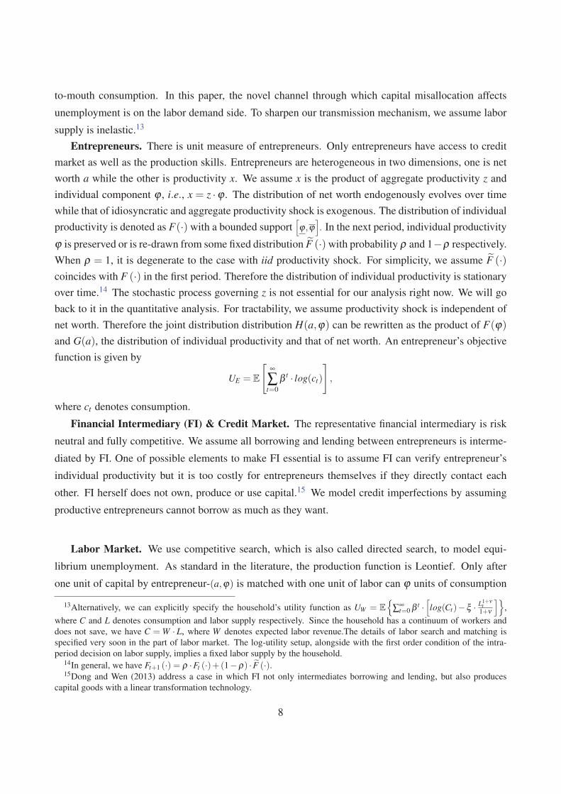
subject to
p(θ (ϕ,W )) ·w(ϕ,W ) =W, (2.3)
where W (ϕ) =W (ϕ ′)≡W denotes the expected wage revenue by going to sub-market ϕ,ϕ ′ ∈ΦA ⊆Φ,
where ΦA denotes the set of entrepreneurs active in production. We characterize ΦA in Section 2.4, and
right now treat it as given. We now characterize the endogenous wage offer in active sub markets ΦA.
Proposition 1. (Wage Scheme)
1. Given W , the market tightness in any active sub-market ϕ ∈ ΦA is determined by
q′ (θ (ϕ)) =Wϕ. (2.4)
2. The wage scheme and expected capital revenue obtained from sub-market ϕ ∈ ΦA is given by
w(ϕ ,W ) =W
p(θ (ϕ))(2.5)
π (ϕ ,W ) =[q(θ (ϕ))−θq′ (θ (ϕ))
] ·ϕ.3. Comparative statics:
∂π (ϕ,W )
∂ϕ> 0,
∂π (ϕ ,W )
∂W< 0,
∂θ (ϕ,W )
∂ϕ> 0,
∂θ (ϕ,W )
∂W< 0,
∂q(θ (ϕ,W ))
∂ϕ> 0,
∂q(θ (ϕ,W ))
∂W< 0.
The marginal value of being matched with labor increases with the productivity. Therefore the wage
scheme increases with productivity. In turn, entrepreneurs with higher productivity enjoy a higher job-
filling rate. Therefore high-productivity entrepreneurs are more efficient in both extensive and intensive
margins. This observation is the key to understanding the general-equilibrium effect of capital misal-
location on unemployment in next section. Finally, Proposition 1 shows the expected capital revenue
increases with productivity. This property, like that in Melitz (2003), delivers a cut-off point for active
entrepreneurs and greatly simplifies our analysis in Section 2.4.
2.3 Entrepreneur’s Constrained Optimization
At the beginning of each period, entrepreneurs reply on two pieces of public information to decide
whether to be active or not in production. One is the individual state variable, which includes net worth
a and productivity ϕ . The other one is the aggregate state variable X = (λ ,η ,z,F (ϕ) ,G(a)). Assume
some entrepreneur uses k units of capital for production. Then we use b ≡ k− a to denote the external
funding. That b < 0 means net lending. Since the production function is Leontief, active entrepreneurs
posts their wage scheme w(ϕ) for every unit of capital at sub market ϕ ∈ ΦA. For notational ease, we
11

replace π(ϕ,W ) with π (ϕ) in the rest of the paper. Assume the law of large numbers holds here. Then
the total capital revenue is Π(k,ϕ) = π(ϕ) · k for the entrepreneur with productivity ϕ and using k units
of capital for production. We model credit frictions with the simplest collateral constraint, i.e., k ≤ λ ·a,
where k and a denotes the total capital available and own net worth respectively, and λ the exogenous
financial shock to the credit market. If λ = 1, the credit market collapses and entrepreneurs are in
autarky. If λ = ∞, the credit market is complete since the collateral constraint would never be binding.
Finally the constrained optimization of entrepreneur-(a,ϕ) is formulated as below.
V (a,ϕ;X) = max{
log(c)+β ·E[V (a′,ϕ ′;X ′) |X]} (2.6)
subject to
r ·b+ c+ i = Π(k,ϕ) = π(ϕ) · k (2.7)
a′ = (1−δ ) ·a+ i (2.8)
b = k−a (2.9)
k ≤ λ ·a (2.10)
k ≥ 0 (2.11)
Equation (2.7) is the budget constraint with Π(k,ϕ) being the capital revenue, r ·b the debt repayment,
c the consumption and i the investment for next period. Equation (2.8) is the accounting identity on
investment, net worth and the total capital obtained for production. Equation (2.9) is the definition on
external funding b. Equation (2.10) is a collateral constraint, in which the maximum available capital
is proportional to entrepreneur’s own net worth. The collateral constraint k ≤ λ ·a implies the leverage
ratio is the same across heterogeneous entrepreneurs, and has nothing to do with interest rate. This is
purely for tractability.21 As emphasized by Moll (2012), it is the linearity of collateral constraint that
guarantees tractability. Equation (2.11) denotes a no-short-selling constraint.
We use the simplest form of collateral constraint. Unlike Kiyotaki-Moore (1997), we eliminate
the price effect. As shown in Section 3, this simplification will illustrate the unemployment effect of
capital misallocation in a transparent way. Moreover, we can anticipate that the additional consideration
of price effect would strengthen the novel channel proposed there. Secondly, credit imperfections are
characterized by the above collateral constraint in a reduced-form way. There are several alternatives
with micro-foundation to support the linear form of collateral constraint. In addition to the limited
liability proposed by Kiyotaki and Moore (1997), we can also obtain the linearity by considering costly
state verification by Williamson (1987) and Bernanke and Gertler (1989), or moral hazard by Holmstrom
and Tirole (1997). Finally, our baseline only takes into account credit frictions and labor search frictions.
This would help us focus on the unemployment effect of worsening capital misallocation in the simplest
21We also try a complicated version in which the collateral constraint is related to interest rate and productivity hetero-
geneity. The result is still tractable at both micro and aggregate levels. It is available upon request.
12

and most clear way.
2.4 Credit Market
We use this part to characterize under what conditions the collateral constraint is binding for en-
trepreneurs heterogeneous in net worth and productivity. Denote Π(k,ϕ) as the capital revenue by
entrepreneurs with productivity ϕ and using k units of capital for production. Based on Proposition 1
and assume the law of large number applies, we know the capital revenue is linear in k, and
Π(k,ϕ) = π (ϕ) · k = kq(ϕ)ϕ − kθ (ϕ)W, (2.12)
Then the constrained optimization by entrepreneur-(a,ϕ) can be simplified as below.
V (a,ϕ;X) = max{
log(c)+β ·E[V (a′,ϕ ′;X ′) |X]}subject to
c+a′ = [r+(1−δ )] ·a+max{π(ϕ)− r, 0} · kk ∈ [0, λ ·a] , λ ∈ (1,∞)
The entrepreneur-(a,ϕ) can always receive the capital revenue [r+(1−δ )] ·a by making a deposit
to the financial intermediary. Additionally, if the entrepreneur uses k units of capital for production,
then the net gain is π(ϕ)− r, where π(ϕ) and r denotes the expected revenue and the opportunity cost
of using one unit of capital for production. Therefore the option value for each unit of capital held
by entrepreneur with productivity ϕ is max{π(ϕ)− r, 0}. In turn, we follow Buera and Moll (2013) to
define the return premium as RP ≡ E [max(π (ϕ)− r, 0)]. If there is no credit friction or no productivity
heterogeneity, then the return premium is simply zero. Given the individual capital demand k (ϕ,a), the
clearing condition in the credit market is then obtained by
ˆ ˆk(ϕ,a) ·h(ϕ,a)dϕda =
ˆ ˆa ·h(ϕ,a)dϕda. (2.13)
We then use the following lemma to characterize the individual capital demand.
Lemma 1. (Capital Demand and Cash Holding) Capital demand by entrepreneur-(a,ϕ) conforms to
a corner solution, i.e.,
k(ϕ,a) =
⎧⎨⎩0 if ϕ ∈[ϕ, ϕ
]λ ·a if ϕ ∈ [ϕ,ϕ]
,
where the cut-off value ϕ is determined by
π (ϕ) = r, (2.14)
13

and the ratio of cash holding to assets is λ · [1−q(ϕ)].
Denote the aggregate net worth as K ≡ ´ a ·dG(a). The above lemma suggests the measure of capital
in sub market ϕ is
v(ϕ) =[ˆ
k (ϕ,a)dG(a)]· f (ϕ) ·1{ϕ≥ϕ} = λK f (ϕ) ·1{ϕ≥ϕ}. (2.15)
Entrepreneurs with high enough productivity produce and hit a binding collateral constraint. The
rest prefer lending in the credit market. The property of choosing corner solutions is due to the linearity
of capital gains. Besides, this lemma immediately reveals that the set of active entrepreneurs is ΦA =
{ϕ|ϕ ≥ ϕ}. It is worth noting that, although active entrepreneurs want to borrow as much as they want
with a binding collateral constraint, the equilibrium leverage ratio used for production is λ ·q(ϕ) rather
than λ in the presence of labor search frictions. Consequently cash holding emerges in equilibrium. The
ratio of cashing hold to assets decreases with productivity. This is determined by the use of capital with
labor search frictions, which is illustrated as follows.
Corollary 1. (Double Selection on Capital Use) The productivity distribution of active entrepreneurs
and that of matched entrepreneurs are
FA(ϕ) =F(ϕ)−F(ϕ)
1−F(ϕ), FM(ϕ) =
´ ϕϕ q(ϕ ′) ·dF(ϕ ′)´ ϕϕ q(ϕ ′) ·dF(ϕ ′)
,
and FM(ϕ)< FA(ϕ)< F(ϕ).
( )
( )( )
Figure 2.3: Double Selection of Capital Use
It is worth noting that the equilibrium productivity distribution is FM(ϕ) rather than FA(ϕ). The
latter is the truncated distribution in the first step. As proved in Proposition 1, the job-filling rate of
active entrepreneurs increases their individual productivity. As a result, the equilibrium productivity
distribution is obtained after the selection in the second step, which reflects in the weight q(ϕ) in the
above equation of FM(ϕ). We illustrate the relationship of these three distributions in Figure (2.3). In
the end, we obtain the policy function of entrepreneur-(a,ϕ) in partial equilibrium.
14

Corollary 2. (Individual Policy Function) Given the aggregate state variable X , the consumption and
saving by entrepreneur-(a,ϕ) is linear with her own net worth.
at+1 (at ,ϕt) = β ·Ψt (ϕ) ·at
ct (at ,ϕt) = Ψt (ϕ) ·at −at+1 (at ,ϕt) ,
where Ψt (ϕ)≡ λt ·max{πt (ϕ)− rt , 0}+[rt +(1−δ )].
The linearity of policy function admits a tractable aggregation.22 Therefore we can keep track of the
endogenous evolution of the distribution without resorting to purely numerical work like Krusell and
Smith (1998). The linear property of policy function makes it easy for us to connect with recent literature
on credit frictions. For example, Wang and Wen (2012) develop an incomplete credit market model with
heterogeneity in investment efficiency as well as with partial irreversibility such that a′ ≥ λI · (1−δ ) ·a.
Notice that λI = 0 and λI = 1 denote the cases with perfect reversibility and complete irreversibility
respectively. Based on the above corollary, the individual policy function is still tractable with the
additional constraint of partial investment irreversibility upon our framework. In this scenario, the
intertemporal decision would be adjusted as
at+1 (at ,ϕt) = max{β ·Ψt (ϕ) ,λI · (1−δ )} ·at .
3 Equilibrium
We have so far addressed the decisions of all agents in partial equilibrium. We summarize the key results
in Figure (3.1).This section is devoted to exploring general equilibrium of our model with with heterogeneous en-
trepreneurs, and with credit and labor search frictions. We characterize not only the equilibrium in each
period, but also the transition dynamics. We start with defining the recursive competitive equilibrium as
below.
Definition 1. (Recursive Competitive Equilibrium) A recursive competitive equilibrium consists of
1. labor supply l(ϕ), capital v(ϕ) and market tightness θ(ϕ) at active sub-market ϕ ∈ ΦA,
2. a set of price functions, including the interest rate r, the wage scheme w(ϕ) and the expected labor
gain from sub-market W (ϕ) in active sub-market ϕ ∈ ΦA ,
3. a set of individual policy functions, including consumption c, debt b, and net worth for next period
a′,22In the presence of partial irreversibility, the policy function is adjusted as at+1 (at ,ϕt) = max{β ·Ψt (ϕ) , λI,t · (1−δ )} ·
at . Thus the linearity property is preserved.
15

Entrepreneur A: productivity ;wage posting ( ) at sub-market .
Entrepreneur B: productivity ;wage posting ( ) at sub-market .
Entrepreneurs are active and borrow if .
Entrepreneurs are inactiveand lend if < .
Financial intermediaryEntrepreneurs
Workers
Figure 3.1: Decision Rules of All Agents
4. the value function V (a,ϕ),
5. the law of motion for the aggregate state variable X = (z,λ ,η ,F(ϕ),G(a)), such that,
• given X and W the market tightness θ(ϕ) = l(ϕ)/v(ϕ) is determined by Equation (2.4), v(ϕ) by
Equation (2.15) and wage w(ϕ) by Equation (2.5),
• given X , the cut-off point, ϕ , the interest rate r, and the expected wage revenue W are jointly
determined by Equations (2.14), (2.13), and (2.1),
• c(a,X) and a′(a,X) is the solution to the entrepreneur’s dynamic optimization, and the value
function V (a,X) is obtained with c(a,X) and a′(a,X),
• the credit market clears as in Equation (2.13).
3.1 Equilibrium Wedges
We first address the social planner’s problem. More specially, there is only labor search friction in the
benchmark. Then the problem is formulated as below.
Y ∗ = max{v(ϕ),l(ϕ)}
ˆΦ
z ·ϕ ·m(v(ϕ), l(ϕ))dϕ
16

subject to
ˆΦ
v(ϕ)dϕ ≤ K ≡ˆ ˆ
a ·h(ϕ,a)dϕdaˆ
Φl(ϕ)dϕ ≤ L
v(ϕ), l(ϕ) ≥ 0,
where v(ϕ) and l (ϕ) denotes the measure of capital and labor in sub-labor market ϕ . We summarize
the key results as below.
Lemma 2. (Benchmark) If the matching function is constant return to scale, the most efficient alloca-
tion is that all capital and labor are assigned to the most productive entrepreneurs, i.e., v∗(ϕ) =K ·1{ϕ=ϕ},
l∗(ϕ) = L ·1{ϕ=ϕ}, Y ∗ = z ·ϕ ·m(K,L), N∗ = m(K,L), u = 1− NL∗, and ALP∗ ≡ Y ∗
N∗ = z ·ϕ .
First, the efficient allocation can be realized if all firms have to post a unique wage. The Bertrand
competition would then drive up the wage to z ·ϕ . Secondly, the benchmark results on allocation should
be treated with caveat. If we use the span-of-control model by Lucas (1978), then it is not necessarily
true all resources should be used by the most productive firms.
In the rest of this section, we characterize the equilibrium allocation of the decentralized economy.
To start with, we make an assumption as below.
Assumption 1. ϒ(ϕ)≡EF
(ϕ
1−γγ |ϕ∈[ϕ,ϕ]
)[EF
(ϕ
1γ |ϕ∈[ϕ,ϕ]
)]1−γ strictly increases with ϕ ∈(
ϕ,ϕ)
for γ ∈ (0,1)
This assumption is reasonable in the sense that it is held with Uniform distribution, Power distribu-
tion, and Upper Truncated Pareto distribution, all of which are frequently used in the literature.23 As
emphasized in Section 2, we assume the upper bound of productivity distribution is less than infinity. We
didn’t consider Pareto distribution in the theoretical or quantitative parts of our paper. On the one hand,
the boundedness of ϕ is of theoretical importance. When the credit market is complete, i.e., λ → ∞,
only the most productive entrepreneurs would take over the production. Models with a Pareto distribu-
tion would not be well defined in the extreme scenario, as emphasized by Moll (2012) and Wang and
Wen (2013), who addresses heterogeneity in productivity and investment efficiency respectively with
an incomplete financial market. On the other hand, our key channel through which credit imperfections
affect unemployment would heavily depend on the above assumption. However ϒ(ϕ) would be purely
23As shown in Appendix D, the above assumption is equivalent to assuming, for all ϕ ∈(
ϕ,ϕ)
, we have
EF
[(ϕϕ
) 1γ|ϕ ∈ (ϕ,ϕ)
]·{
1−(
1
γ
)·[
1−F (ϕ)ϕ · f (ϕ)
]}≤ 1.
17

constant if we adopt a Pareto distribution, and thus the transmission mechanism would be shut down
in equilibrium. Therefore we instead use a Power distribution with a normalized support [0,1] in the
coming quantitative analysis.24
Following the literature on business cycle accounting, such as Chari, Kehoe and McGrattan (2007),
we characterize allocation and wedges of the decentralized economy in general equilibrium as below.
Proposition 2. (Wedges in General Equilibrium) Given the aggregate state variable X ,
1. the cut-off point ϕ increases with λ such that limλ→1
ϕ = ϕ and limλ→∞
ϕ = ϕ .
2. the aggregate output and the total matched workers are
Y = (1− τy) ·Y ∗ = (1− τy) ·ϕ ·m(K,L)
N = (1− τn) ·N∗ = (1− τn) ·m(K,L)
where
1− τy = Λ(λ )≡ EF
[(ϕϕ
) 1γ|ϕ ∈ [ϕ,ϕ]
]γ
∈ (0,1)
1− τn = Ω(λ )≡EF
(ϕ
1−γγ |ϕ ∈ [ϕ,ϕ]
)[EF
(ϕ
1γ |ϕ ∈ [ϕ,ϕ]
)]1−γ ∈ (0,1) .
both of which increases with λ , and limλ→∞
τy = limλ→∞
τn = 0.
3. the average labor productivity, ALP ≡ YN , and unemployment, u ≡ 1− N
L , is25
ALP =(1− τal p
) ·ALP∗ = EFM (ϕ)
u ≡ (1+ τu) ·u∗ = u∗+ τn · (1−u∗) (3.1)
where
1− τal p =1− τy
1− τn= ϒ(λ )≡
EFi
[ϕ
1γ
i |ϕi ∈ [ϕi,ϕ i]
]EFi
[(ϕ iϕi
)·ϕ
1γ
i |ϕi ∈ [ϕi,ϕ i]
] ∈ (0,1)
1+ τu = 1+ τn ·(
1−u∗
u∗
)∈ (1,∞) .
24Uniform distribution is a special case of Power distribution. We use uniform distribution as an example in our theoretical
analysis since it is a perfect candidate to exercise mean preserving spread. We then calibrate the parameters of Power
distribution in the quantitative part. We also tried the Upper Truncated Pareto distribution.25We use λ = ∞ as the limit case for our theoretical analysis. If we use some λ < ∞ instead as the limit scenario, then the
formula between u and u∗ is adjusted as u = u+[
1− Ω(λ )Ω(λ)
]· (1−u), where u ≡ 1−Ω
(λ)·m(K
L ,1).
18

4. the wedge to the expected labor revenue is zero, i.e., W = ∂Y∂L while the wedge to the interest rate
is
r = (1− τr) ·(
∂Y∂K
)
where 1− τr ≡ 1
EFi
[(ϕi/ϕi)
1γ |ϕi∈[ϕi,ϕ i]
] , which increases with λ , and limλ→∞
τr = 0.
5. the equilibrium labor supply and the corresponding wage offer in sub market ϕ is
l (ϕ)L
=
[ϕ
Λ(λ )
] 1γ·[
v(ϕ)K f (ϕ)
]w(ϕ) = (1− γ) ·ϕ ·1{ϕ≥ϕ(λ )},
and the cumulative distribution is Fw (ω)≡ Pr{w ≤ ω}= FM
(ω
1−γ
), where FM (·) denotes the equi-
librium productivity distribution of the capital they are matched with labor.
First, both ALP and N increase with λ . Therefore credit imperfections affects the output only
through lowering capital misallocation, i.e., the decrease of ALP, but also by alleviating labor misal-
location, i.e., the increase of employment. The former and latter denotes the intensive and extensive
margins respectively. Therefore our model offers a novel channel through which a credit crunch gen-
erates an amplification effect on output. We further illustrate this result in the quantitative exercise at
Section 4.
Secondly, given ϕ ≥ ϕ , both v(ϕ) and l (ϕ) increases with λ . However, as shown in the above propo-
sition, l (ϕ) does not increase as much as v(ϕ) does. Therefore the market tightness θ (ϕ) ≡ l (ϕ)/v(ϕ)
and the associated job-filling rate q(ϕ) decreases with λ in general equilibrium. That is, as more capital
is concentrated at the top end, the market tightness tends to be less favorable to firms.
Thirdly, Proposition 2 provides a micro-foundation for Cobb-Douglas aggregation. In turn, equilib-
rium TFP is defined as
T FP(λ ,η ,z)≡ YKγL1−γ = [ALP(λ ,z)] · [Ω(λ ) ·η ] , (3.2)
which is determined by aggregate productivity and frictions to credit and labor markets. Therefore
credit imperfections affect equilibrium TFP at intensive margin (capital misallocation) as well as ex-
tensive margin (employment). We can also characterize TFP wedge as T FP ≡ (1− τt f p) ·T FP∗ and thus
τt f p = τy. Moreover, following Lagos (2006), we can alternatively use the finally matched capital and
labor, i.e., LM = KM = N to measure equilibrium TFP. Then we have T FP ≡ YKγ
ML1−γM
= YN = ALP, which
is affected by both z and λ . However, it is independent of η since matching efficiency only affects
matched capital and labor.
We have characterized at the end of Section 2 the intertemporal decision of individual entrepreneurs.
We close this part by characterizing the aggregate transition dynamics.
19

Corollary 3. (Aggregate Transition Dynamics)
Kt = β · [γ ·Yt +(1−δ ) ·Kt ] .
Gt+1(a) =
ˆGt
(a
β ·Ψt (ϕ)
)·dFt(ϕ).
The evolution of aggregate capital stock behaves like a Solow model in which output is subject to a
tax rate (1− γ) and the saving rate is constant. On the one hand, Cobb-Douglas matching function in all
sub-labor markets suggests a fixed split of output between entrepreneurs and workers. Since we assume
workers cannot have access to financial market, only entrepreneurs makes intertemporal decision. On
the other hand, we use log-utility, which exactly cancels income and substitution effects and implies a
fixed saving rate.
3.2 The Unemployment Effect of Credit Imperfections
The key theoretical contribution of this paper is to show that a credit crunch, i.e., a decrease in λ ,
lowers aggregate matching efficiency. We use this part to present the details of this novel transmission
mechanism. As shown in the proof of Proposition 2, equilibrium employment can be formulated as
N = EF [q(ϕ)|ϕ ≥ ϕ] ·K, (3.3)
where K denotes the aggregate capital supply and q(ϕ) the job-filling rate in sub-labor market ϕ . In turn
we obtain the employment effect of credit imperfections as below.
∂N∂λ
=
{(∂EF [q(ϕ)|ϕ ≥ ϕ]
∂ ϕ
)·(
∂ ϕ∂λ
)+EF
[∂q(ϕ)
∂λ|ϕ ≥ ϕ
]}·K ≥ 0 (3.4)
First, the increase of λ drives up the interest rate r and thus the cut-off value ϕ . Then more capital
is redistributed from low-productivity to high-productivity entrepreneurs. As proved in Section 2.2,
the entrepreneur’s job-filling rate q(ϕ) increases with ϕ . Therefore the direct effect, which is shown
in the first item of the right hand of Equation (3.4), is that the employment increases. We call it the
selection effect. However, holding everything else unchanged, when more capital is concentrated to the
hand of high-productivity entrepreneurs, the job-filling rate of all active entrepreneurs tends to decrease.
Although labor supply responds to the increase of λ , the concavity of matching function suggests l (ϕ)
does not change as much as v(ϕ) and thus q(ϕ) decreases with λ in general equilibrium. This can be
verified from the above proposition. This indirect general equilibrium effect is labeled as congestion
effect, which is shown in the second item of right hand of Equation (3.4). As proved in the Appendix D,
the selection effect dominates the congestion effect under Assumption 1.
20
0 0.2 0.4 0.6 0.8 10.84
0.86
0.88
0.9
0.92
0.94
0.96
0.98
1
1.02
σ/μ: Mean Preserving SpreadΩ
: E
ndo
Mat
chin
g E
ffic
ienc
y
λ=1 (Autarky)λ=1.5λ=∞ (Complete credit mkt)
1 2 3 4 50.84
0.86
0.88
0.9
0.92
0.94
0.96
0.98
1
1.02
λ: Leverage Ratio
Ω:
End
o M
atch
ing
Eff
icie
ncy
σ/μ=0 (no hetero.)σ/μ=0.3σ/μ=0.9
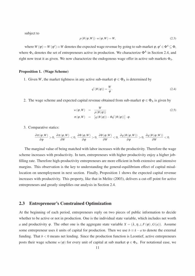
Figure 3.2: Left Panel: (Ω,λ ); Right Panel:(
Ω, σμ
); ϕ U∼ [μ −σ ,μ +σ ].
As suggested by Equation (3.1), productivity heterogeneity with an incomplete credit market does
matter for matching efficiency in the labor market. Such kind of effect cannot be obtained in a standard
framework with a representative firm and worker. For example, the seminal work by Wasmer and
Weil (2004) introduce credit frictions into an otherwise standard Diamond-Mortensen-Pissarides model.
They model credit frictions with a matching function between a representative firms and bank. When
credit frictions worsen, which could be driven by the decrease of matching efficiency between firms and
banks, affect equilibrium unemployment in steady state. However, unlike our heterogeneity model, the
Beveridge curve in their works does not move with such kind of disruption in credit market.
Finally, endogenous matching efficiency contributed by credit imperfections, Ω, is affected not only
by λ , but also by productivity distribution. Given any distribution F (·), we have shown Ω increases
with λ . We close this part by addressing the implications of an MPS (mean preserving spread) of
F (·) for Ω. The general discussion is beyond this paper. We instead use a special case to illustrate
the idea by assuming F (·) is a Uniform distribution with support [μ −σ ,μ +σ ] and σ ∈ [0,μ]. We
use uniform distribution since it is a perfect candidate to perform MPS. More specifically, given any
λ , we can check the effect of σμ on Ω. The right panel of Figure (3.2) implies an MPS increases
unemployment. Our exercise with MPS is related to the recent literature on the relationship between
adverse selection and output fluctuation, see Kurlat (2012) and Bigio (2013), among others. We all show
that an MPS depresses the output. There are mainly two key differences. First, information asymmetry
is indispensable in their works while we perform the MPS under complete information. Secondly,
they assume a frictionless labor market while we assume labor search frictions and an MPS drives up
unemployment.
21

3.3 Unemployment Decomposition
Motivated by the channel through which credit imperfections affect labor market, we make a theoretical
decomposition for unemployment in this part. In particular, we explore how much credit imperfections
and the classic labor search frictions add to unemployment respectively.
Steady State
Using Corollary 3 reaches steady-state unemployment as below.
uss = 1− [Ω(λss) ·ηss]1
1−γ ·[
γ ·ALP(λss,zss)
1/β −1+δ
] γ1−γ
, (3.5)
As indicated by Equation (3.5), the credit friction λ plays two roles in determining unemployment in
steady state. On the one hand, the increase of λ contributes to a higher TFP, which in turn suggests
a higher capital stock in steady state. Therefore unemployment tends to decrease. On the other hand,
given any level of capital stock, endogenous matching efficiency would also increase with λ and thus
lower unemployment. In the end we reach the general equilibrium effect of credit imperfections on
unemployment in the steady state as below.
(uss −u∗ss) = (uss − u)+(u−u∗ss) ,
where uss and u∗ss denotes respectively the steady state unemployment with a steady state λ and
with a “high enough” λ . The difference between uss and u∗ss is defined as unemployment contributed
by credit imperfections in the steady state. Furthermore, u is denoted as unemployment implied by a
higher λ , but the matching efficiency is controlled constant. That is, u is the steady state unemployment
with a higher capital stock implied by an improvement of capital reallocation, but the efficiency of labor
reallocation is held unchanged. We have formulated uss in Equation (3.5). In turn, u∗ss and u are given
as below.
u∗ss ≡ 1− [Ω(λ ∗) ·ηss]1
1−γ ·[
γ ·ALP(λ ∗,zss)
1/β −1+δ
] γ1−γ
u ≡ 1− [Ω(λss) ·ηss]1
1−γ ·[
γ ·ALP(λ ∗,zss)
1/β −1+δ
] γ1−γ
,
where λ ∗ denotes a “high” financial development. We have two alternative candidates for λ ∗, one is
∞ while the other one is max{λt}. The former is mainly of theoretical interest. As proved in Proposition
2, endogenous matching efficiency by credit imperfections would converge to the maximum level when
λ ∗ approaches to the infinity. The latter is instead used for the quantitative analysis to come.
22

Non Steady State
In every period we have u = 1−Ω(λ ) ·m(KL ,1). That is, the total matching efficiency is the product of
that contributed by financial friction and that by labor search frictions, i.e., η = Ω(λ ) ·η . Then we have
u = u∗∗+(
limλ→λ ∗u−u∗∗
)+
(u− lim
λ→λ ∗u)≡ u∗∗+uη +uλ ,
where u∗∗ = max{
1− KL ,0}
and limλ→λ ∗
u = 1−Ω(λ ∗) ·m(KL ,1)
denotes respectively the efficient unem-
ployment and the unemployment without credit imperfections. First, data on KL suggest u∗∗ = 0. Then
we break down unemployment into the two parts as follows, one of which is due to the classic search
friction while the other due to credit imperfections. We denote them as uη and uλ respectively. In turn,
we define the explanatory power of credit imperfections on unemployment as χ ≡ uλ
u . Given K, ag-
gregate productivity shock z does not directly affect unemployment since z has nothing to do with the
equilibrium aggregate matching efficiency. Therefore the decomposition exercise does not involve z.
However, z exerts a dynamics effect on unemployment because aggregate productivity shock plays a
role in equilibrium TFP, which in turn influences the speed of capital accumulation.
Finally, we get that ∂ χ∂λ < 0,
∂ χ∂η > 0,
∂ 2χ∂λ∂η < 0 and ∂ χ
∂λ ∗ > 0. The increase of λ suggests an amelioration
of capital misallocation, and thus the role of credit imperfections in explaining unemployment decreases.
As a duality, we have∂ (1−χ)
∂η < 0, which immediately translates into∂ χ∂η > 0. Furthermore these exists
an interaction effect. These properties turn out helpful in interpreting results, mainly Figure (4.6), in
Section 4.3. We illustrate the key results on χ in Figure (3.3).
( , )
Figure 3.3: Explanatory Power of Credit Imperfections for Unemployment
3.4 The Relationship to A Model with Only Credit Frictions
We have finished the specification and characterization of our model with credit and labor-search fric-
tions. Comparing the equilibrium of the decentralized economy with the benchmark with only search
23

frictions delivers Proposition 2. We address the wedges to productivity, employment, average labor
productivity, unemployment rate and factor prices there.
We use this part to propose an alternative benchmark in which there is no labor search friction
but just credit friction. More specifically, we compare our model with Moll (2013). We establish the
connection as below.
Proposition 3. (Comparison with A Model with Only Credit Frictions) The heterogeneous-entrepreneurs
model with both search frictions in the labor market with matching function m(l(ϕ),v(ϕ))=η ·v(ϕ)γ l(ϕ)1−γ ,
and credit frictions in the form of a collateral constraint k ≤ λ · a delivers the same output aggregation
and transition dynamics on F(ϕ), G(a) and K with the model with the following characteristics:
1. The production function by entrepreneur-(a,ϕ) is y(ϕ,a) = ϕ ·m(k(ϕ,a), l(ϕ,a)).
2. The labor market is frictionless in each period, i.e., there exists a unique and publicly displayed
wage w such that labor supply equals demand. Unemployment is then zero by definition.
3. The credit market is subject to a collateral constraint, i.e., k ≤ λ ·a.
Moreover, we can use the model with only financial friction to recover unemployment in the model with
dual frictions as u = 1− YL·EFM (ϕ) .
The key message from this proposition is that, our model with two layers of frictions behave as
if there exist only credit imperfections, and the Leontief production function is replaced by the Cobb-
Douglas. On the other hand, we can interpret the heterogeneous model with only credit frictions as a
model with both credit and labor search frictions, and the Cobb-Douglas production function is decom-
posed into a Leontief production and an associated Cobb-Douglas matching function.
3.5 Job Destruction and Firm Growth
We have assumed throughout the paper that all matched relationship between firms and workers is
terminated after production. This assumption greatly simplifies our analysis since entrepreneur are
heterogeneous in only two dimensions. The associated cost is that, the ratio of job destruction to total
employment is 100% at the end of each period. To partially fix this problem, we redefine job destruction
in terms of net flow.
Nt+1 = Nt − JDt+1 + JCt+1, (3.6)
24

where
Nt ≡ˆ ˆ
ltht(ϕ,a)dϕda = Ω(λt) ·mt(Kt ,Lt)
JDt+1 ≡ˆ ˆ
max{
lt − lt+1, 0}
ht(ϕ,a)dϕda
JCt+1 ≡ˆ ˆ
max{
lt+1 − lt , 0}
ht(ϕ,a)dϕda
and lt denotes the finally matched workers, and h(ϕ,a) the joint distribution of productivity and
net worth. Given Nt ,Nt+1 and JDt+1, we can then calculate JCt+1 from Equation (3.6). Moreover, in
each period, given the aggregate state variable Xt , we can pin down Nt . Therefore it remains for us to
characterize JDt+1. We summarize the key results as below.
Corollary 4. (Job Creation and Destruction) In each period, job destruction can be formulated as
JDt+1 =
[ˆmax(Δt,t+1 (ϕt) , 0) ·dF(ϕt)
]·Kt+1.
where
Δt,t+1 (ϕt)≡ λt ·1{ϕt≥ϕt}qt (ϕt)−λt+1βΨt (ϕt) ·[
ρ ·1{ϕt≥ϕt+1}qt+1(ϕt)+(1−ρ) ·ˆ
Φ1{ϕ≥ϕt+1}qt+1(ϕ) ·dF(ϕ)
].
Using the corollary immediately suggests that job creation and job destruction in steady state is
JD = JC =
[ˆ ϕ
ϕmax
{1−βΨ(ϕ) ·
[ρ ·q(ϕ)+(1−ρ) ·
(N
λK
)], 0
}dF(ϕ)
]·λK.
where K and N in steady state are
K =
[γ ·T FP(λ ,η ,z)1/β − (1−δ )
] 11−γ
·LN = Ω(λ ) ·m(K,L).
We close the theoretical part with a discussion on the implications of this model for firm-level
growth.
Corollary 5. (Firm Size and Growth Rate)
1. The firm size of entrepreneur-(a,ϕ), measured by capital holding k and employee numbers n, are
k(a,ϕ) = λa ·1{ϕ≥ϕ}
n(a,ϕ) = λq(ϕ)a ·1{ϕ≥ϕ}.
25

2. The growth rate of capital and employment is,
E
[kt+1
kt|(kt ,ϕt ;Xt)
]= β ·
(Ψt(ϕt)
λt
)·E{[
ρ ·1{ϕt≥ϕt+1}+(1−ρ) · (1−F (ϕt+1))]·λt+1|(ϕt ,Xt)
}E
[nt+1
nt|(nt ,ϕt ;Xt)
]= β ·Ψt(ϕt)
(λt+1
λt
)⎡⎣ρ ·(
qt+1(ϕt)
qt(ϕt)
)+(1−ρ) ·
⎛⎝´ ϕϕt+1
q(ϕt+1)dF(ϕt+1)
qt(ϕt)
⎞⎠⎤⎦ .Our model predicts that the growth rate has nothing to do with capital or employment itself. This is
purely because of the linearity of policy function of individual entrepreneurs. Moreover, the heteroge-
neous growth rate connects our paper with the empirical and theoretical works on the volatility of firm
growth rate, such as that by Wang and Wen (2013), etc.
4 Quantitative Analysis
In this section we confront the model with data by quantifying the unemployment effect of capital mis-
allocation due to credit imperfections. We calibrate the model on US economy and then back out the
realization of three pieces of aggregate shocks. Then we estimate the stochastic process of these three
shocks and do the impulse response exercise. Furthermore, we decompose unemployment into two
parts, one is due to credit imperfections and the other due to the classic labor search frictions. Unem-
ployment decomposition is considered not only for the business cycles between 1951Q4 and 2011Q4,
but also for the recent financial crisis. Finally, we discuss which shocks are most essential in terms of
their aggregate and disaggregate implications.
4.1 Calibration
Data are of quarterly frequency. Details on the criterion of data use, data description and calculation are
documented in the Appendix A. The date horizon ranges between 1951Q4 to 2011Q4.26
Calibration
Assume the individual productivity component follows a Power distribution, i.e., F (ϕ) = ϕ1ε with the
support[ϕ,ϕ
]= [0,1] and ε > 0. Notice that the lower bound is truncated at zero since productivity is non-
26The data start with 1951Q4 since it is the earliest date in the Flow of Funds Account such that the data on external
funding on non-financial assets are available. The date ends with 2011Q4 since this is the last date in which the quarterly
data on non-financial private investment is obtainable. Although the annual data on capital are available till 2012, we have
to use both the annual data on capital and the quarterly data on investment to recover the quarterly data on capital.
26
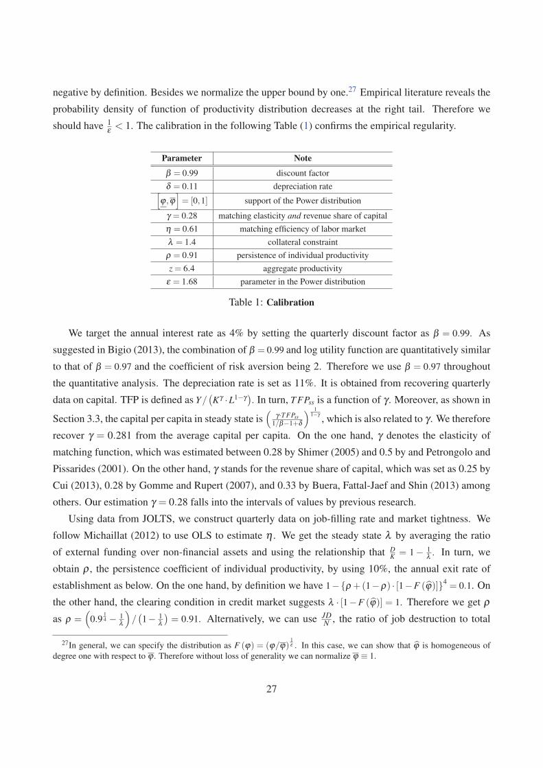
negative by definition. Besides we normalize the upper bound by one.27 Empirical literature reveals the
probability density of function of productivity distribution decreases at the right tail. Therefore we
should have 1ε < 1. The calibration in the following Table (1) confirms the empirical regularity.
Parameter Note
β = 0.99 discount factor
δ = 0.11 depreciation rate[ϕ ,ϕ
]= [0,1] support of the Power distribution
γ = 0.28 matching elasticity and revenue share of capital
η = 0.61 matching efficiency of labor market
λ = 1.4 collateral constraint
ρ = 0.91 persistence of individual productivity
z = 6.4 aggregate productivity
ε = 1.68 parameter in the Power distribution
Table 1: Calibration
We target the annual interest rate as 4% by setting the quarterly discount factor as β = 0.99. As
suggested in Bigio (2013), the combination of β = 0.99 and log utility function are quantitatively similar
to that of β = 0.97 and the coefficient of risk aversion being 2. Therefore we use β = 0.97 throughout
the quantitative analysis. The depreciation rate is set as 11%. It is obtained from recovering quarterly
data on capital. TFP is defined as Y/(Kγ ·L1−γ). In turn, T FPss is a function of γ . Moreover, as shown in
Section 3.3, the capital per capita in steady state is(
γ·T FPss1/β−1+δ
) 11−γ
, which is also related to γ . We therefore
recover γ = 0.281 from the average capital per capita. On the one hand, γ denotes the elasticity of
matching function, which was estimated between 0.28 by Shimer (2005) and 0.5 by and Petrongolo and
Pissarides (2001). On the other hand, γ stands for the revenue share of capital, which was set as 0.25 by
Cui (2013), 0.28 by Gomme and Rupert (2007), and 0.33 by Buera, Fattal-Jaef and Shin (2013) among
others. Our estimation γ = 0.28 falls into the intervals of values by previous research.
Using data from JOLTS, we construct quarterly data on job-filling rate and market tightness. We
follow Michaillat (2012) to use OLS to estimate η . We get the steady state λ by averaging the ratio
of external funding over non-financial assets and using the relationship that DK = 1− 1
λ . In turn, we
obtain ρ , the persistence coefficient of individual productivity, by using 10%, the annual exit rate of
establishment as below. On the one hand, by definition we have 1−{ρ +(1−ρ) · [1−F (ϕ)]}4= 0.1. On
the other hand, the clearing condition in credit market suggests λ · [1−F (ϕ)] = 1. Therefore we get ρas ρ =
(0.9
14 − 1
λ
)/(1− 1
λ)= 0.91. Alternatively, we can use JD
N , the ratio of job destruction to total
27In general, we can specify the distribution as F (ϕ) = (ϕ/ϕ)1ε . In this case, we can show that ϕ is homogeneous of
degree one with respect to ϕ . Therefore without loss of generality we can normalize ϕ ≡ 1.
27

employment, to pin down ρ . The data on JD and N are available at Bureau of Labor Statistics, which
suggest JDN = 1.5% on average. In turn, we have ρ = 0.99.28
When it comes to the estimation on the distribution parameter ε , we can first construct the series
of average labor productivity (ALP) by dividing the output by the employment. Additionally, using
the theoretical results in Section 3 suggests that Ω = T FP/(ALP ·η), which delivers the steady state of
matching efficiency by credit imperfections. Meanwhile notice that Ω is a function of the distribution
parameter ε and that of the steady-state λ . Thus we recover ε = 1.684, which suggests that 1/ε < 1.
Therefore the pdf decreases with productivity and thus is line with empirical regularity. Finally we reach
the steady-state value of z from T FP.
Backing Out Shocks
There are three aggregate shocks in our model, {λt ,ηt ,zt}, which are not directly observable from the
data. We back out these shocks from certain observable time series by following Michaillat (2012). On
the one hand, we have data on i) DtKt
, the external funding over non-financial assets, ii) ALPt , the average
labor productivity, and iii) T FPt . On the other hand, all these three variables of interest are functions of
{λt ,ηt ,zt} in our model, i.e.,
DK
≡´ ∞
0
´ ϕϕ max{k(ϕ,a)−a, 0}h(ϕ,a)dϕda
K=
(DK
)(z,λ ,η)
ALP ≡ YN
= ALP(z,λ ,η)
T FP ≡ YKγ L1−γ = T FP(z,λ ,η).
Furthermore, we can verify the diagonal property holds such that i) DK =
(DK
)(λ ), ii) ALP = ALP(z,λ ),
and iii) T FP = T FP(η ,z,λ ).29 Therefore in each period we can first use(D
K
)t to back out λt . Then zt
could be inferred by jointly using ALPt and the already recovered λt . Finally we use T FPt alongside with
the pairwise estimated value on (λt ,zt) to retrieve ηt . In turn, we obtain their corresponding HP filter in
Figure (4.1).
All these shocks are procyclical in general.30 First, all these three aggregate shocks were signifi-
cantly negative in the recent financial crisis, especially for λ , the shock to the credit market. Moreover,
both λ and η decreases in recessions over the cycles. Notice that we have adopted in a reduced-form
28Since the entrepreneur may lose her productivity with probability (1−ρ) and then may redraw a very low productivity,
she may stop hiring then. Consequently, JDN is a function of ρ in steady state.
29Notice that the ratio of external funding to non-financial asset can be simplified as DK = 1− 1
λ .30The correlation between output and (λ ,η ,z), after HP filtering, is 0.44, 0.64 and 0.21 respectively. Besides, after HP
filtering, corr (λ ,η) = 0.21, corr (λ ,z) =−0.16 and corr (η ,z) =−0.52.
28

HP
Dev
. of L
og( λ
)
1960 1970 1980 1990 2000 2010
-0.01
0
0.01
0.02
0.03H
P D
ev. o
f Log
( η)
1960 1970 1980 1990 2000 2010
-0.02
0
0.02
Date (Quarterly)
HP
Dev
. of L
og(z
)
1960 1970 1980 1990 2000 2010-0.02
0
0.02
Figure 4.1: HP Deviation of Three Shocks
way to model the credit and labor search frictions. On the one hand, as discussed in Section 2.3, the
decrease of λ in recessions may originate from a worsening condition in adverse selection, moral haz-
ard, costly state verification or limited enforcement. On the other hand, the negative shock to η may be
due to the decrease of aggregate matching efficiency, which is in turn caused by some sector-specific
shocks, as shown by Mehrotra and Sergeyev (2012). Alternatively, the decreases of η may stem from
the job polarization proposed by Jaimovich and Siu (2013). The results are mixed when it comes to
the cyclicality of z, aggregate productivity shock. On the one hand, the shocks to z were also negative
in the past three recessions but just opposite for the previous recessions. Our quantitative exercise are
in line with their findings. It is worth noting that, although aggregate productivity z increased in some
recessions, it is not necessarily true that equilibrium TFP also increased correspondingly. As shown in
Figure (4.2), TFP is procyclical with a correlation 0.91 with the output.31
4.2 Impulse Response Exercise and Jobless Recovery
Now we investigate the implications of the aggregate shocks for output and unemployment. We also
address their effects on unemployment decomposition.
31There is seemingly no consensus on the movement of TFP for the recent recession. Petrosky-Nadeau (2012) proposes
a model to explain why TFP increased in this recession. However, as shown in our calculation, TFP, along with the output,
suffered a significant decrease in the past financial recession. This may be due to different measurement methods.
29

Date
HP
Dev
.
1960 1970 1980 1990 2000 2010
-0.03
-0.02
-0.01
0
0.01
0.02
0.03
0.04
RecessionsOutputTFP
Figure 4.2: HP Deviation of TFP
Impulse Response without Correlation or Persistence
We assume these three shocks decrease 1% respectively, but with no persistence or correlation. We
summarize the impulse response of output and unemployment in the first row of each panel in Figure
(4.3). On the one hand, the path of output driven by different shocks shares a similar pattern. On the
other hand, the implications of the shocks are different when it comes to unemployment. The credit
and the labor market shocks exerts a large and immediate response for unemployment. On the contrary,
aggregate productivity affects unemployment one period later and generates a relatively slow recovery.
Since we mainly focus on the connection between credit and labor markets, we devote more analysis
in this line. As illustrated in Section 3.2, credit imperfections lowers aggregate matching efficiency. In
the upper panel of Figure (4.3), we compare the effect of credit crunches in two scenarios, one is with
endogenous matching efficiency while the other is with exogenous matching efficiency. As shown in the
upper panel, endogenous matching efficiency due to credit imperfections amplifies the effect of a credit
crunch for output as well as for unemployment. Moreover, the amplification is quantitatively important.
Now we address the implications of the shocks for unemployment decomposition(uλ ,uη) in the
second row of each panel in Figure (4.3).32 First, although credit and labor shocks have similarity
in their effect on output and unemployment, their predictions on χ , the explanatory power of credit
32The theory formulated in Section 3.3 proposes an unemployment decomposition, i.e., u = uη + uλ , where uη ≡lim
λ→max{λt}u and uλ denotes unemployment contributed by the labor search frictions and credit imperfections respectively.
In turn, we define the explanatory power by credit imperfections to unemployment as χ ≡ uλ/u.
30

0 2 4 6-3
-2
-1
0x 10
-3
Time
(yt-y
ss)/
y ss
endo match efficiencyexo match efficiency(*15)
0 2 4 60
0.5
1
1.5
2
2.5x 10
-3
Time
(ut-u
ss)/
u ss
endo match efficiencyexo match efficiency(*15)
0 2 4 60
1
2
3x 10
-3
Time
uλt
-uλss
uηt
-uηss
0 2 4 6-1
0
1
2
3
4
Time
χt- χ
ss
(a) λ -shock
0 2 4 6-0.01
-0.005
0
Time
(yt-y
ss)/
y ss
0 2 4 60
0.005
0.01
Time
(ut-u
ss)/
u ss
0 2 4 6-5
0
5
10x 10
-3
Time
uλt
-uλss
uηt
-uηss
0 2 4 6-6
-4
-2
0
Time
χt- χ
ss
(b) η-shock
0 2 4 6-0.01
-0.008
-0.006
-0.004
-0.002
0
Time
(yt-y
ss)/
y ss
0 2 4 60
2
4
6x 10
-4
Time
(ut-u
ss)/
u ss
0 2 4 60
1
2
3
4x 10
-4
Time
0 2 4 6-0.25
-0.2
-0.15
-0.1
-0.05
0
Time
χt- χ
ss
uλt
-uλss
uηt
-uηss
(c) z-shock
Figure 4.3: Impulse Response of Shocks (1%) without Correlation or Persistence
31

imperfections on unemployment, are just opposite. These results corroborate the theoretical predictions
in Section 3.3, i.e., ∂ χ∂λ < 0 and
∂ χ∂η > 0. On the one hand, a negative credit shock, i.e., a credit crunch,
boost the importance of credit imperfections in explaining the associated increasing unemployment. On
the other hand, a negative labor shock, i.e., the matching efficiency decreases, puts more emphasize on
the responsibility of labor market itself in worsening unemployment. Moreover, these two shocks exerts
qualitatively asymmetric effect on(uλ ,uη). The former increases both unemployment compositions
while the latter increases uη while decreases with uλ . Finally, as predicted by Section 3.4, aggregate
productivity shock does not directly affect unemployment in the current period. It works through capital
accumulation and thus affects unemployment since the next period. The decrease of capital stock in turn
attenuates the importance of credit imperfects while lends a hand for the role of labor search frictions
in explaining the rising unemployment. However, relative to the previously two shocks, aggregate
productivity shock does not affect χ significantly when it comes to the quantitative concern.
VAR Estimation and Jobless Recovery
We have so far demonstrated the effects of the shocks respectively. Using the HP deviations of these
three shocks delivers the estimation of the VAR process on (λt ,ηt ,zt). We document the estimated
coefficient and variance matrix as below,
⎛⎜⎜⎝βλλ βλη βλ z
βηλ βηη βηz
βzλ βzη βzz
⎞⎟⎟⎠=
⎛⎜⎜⎝0.894 0.147 0.054
−0.120 0.905 −0.004
−0.009 −0.003 0.865
⎞⎟⎟⎠ , Σ =
⎛⎜⎜⎝σ2
λ ρλ z ·σλ σz ρλη ·σλ ση
ρλ z ·σλ σz σ2z ρzη ·σzση
ρλη ·σλ ση ρzη ·σzση σ2η
⎞⎟⎟⎠ ,
where βi j denotes the effect of shock- j on shock-i, and
σλ = 0.0032 ση = 0.0041 σz = 0.0051
ρλ z =−0.0644 ρλη = 0.0899 ρzη =−0.4322
Based on{
βi j}
and Σ, we revisit the impulse response exercise with correlations on the shocks. In
each exercise, the level of initial shock is set as σi with i ∈ {λ ,η ,z}. Then the shocks proceed with the
VAR matrix{
βi j}
. We document the key results in Figure (4.4). As illustrated in the upper and the
middle panel, the shocks to the credit and labor markets generates co-movement of the recovery on out-
put and employment. Therefore(
yt−yssyss
,ut −uss
)is characterized with a perfectly negatively relationship
in the associated figures. In contrast, the shock to aggregate productivity produces a gap (4 quarters)
between the recovery of output and that of employment, which is demonstrated in the lower panel.
32

0 5 10 15 20-1
-0.5
0
0.5
1
1.5x 10
-3
Time
Δy/
y ss
0 5 10 15 20-1.5
-1
-0.5
0
0.5
1x 10
-3
Time
Δu
0 5 10 15 20-1.5
-1
-0.5
0
0.5
1x 10
-3
Time
Δuλ
Δuη
0 5 10 15 20-1.5
-1
-0.5
0
0.5
1
1.5
Time
Δχ
(a) IRF by λ -shock , with innovation magnitude σλ
0 5 10 15 20-5
-4
-3
-2
-1
0
1x 10
-3
Time
Δy/
y ss
0 5 10 15 20-1
0
1
2
3
4
x 10-3
Time
Δu
0 5 10 15 20
0
1
2
3
4
x 10-3
Time
Δuλ
Δuη
0 5 10 15 20-3
-2
-1
0
1
Time
Δχ
(b) IRF by η-shock , with innovation magnitude ση
0 5 10 15 20-6
-5
-4
-3
-2
-1
0x 10
-3
Time
Δy/
y ss
0 5 10 15 20-2
0
2
4
6
x 10-4
Time
Δu
0 5 10 15 20-5
0
5
10x 10
-4
Time
Δuλ
Δuη
0 5 10 15 20-1
-0.8
-0.6
-0.4
-0.2
0
Time
Δχ
(c) IRF by z-shock , with innovation magnitudeσz
Figure 4.4: Impulse Response of Shocks with Correlations
33

When it comes to recessions before 1990s, the recovery on output and employment/unemployment
was on the same pace. However, as shown in Figure (4.5), there exist gaps between output and employ-
ment/unemployment recovery in the past three recessions. It is typically labeled as jobless or sluggish
recovery in the literature. The key message from Figure (4.4) is, aggregate productivity shock is more
likely to generate recovery gaps and thus more responsible to explain the jobless or sluggish recovery
in the recent three recessions. The shocks to the credit and labor markets, on the contrary, synchronize
the recovery of output and employment/unemployment, and are in line with recessions prior to 1990s.
The intuition is, λ and η affect T FP and the equilibrium matching efficiency in the same time, which in
turn determines output and unemployment. However, z only exerts an influence on T FP, but does not
directly relate to the labor market. Consequently the recovery of z immediately improves output while
alleviates unemployment only through increasing capital in the next few periods. In turn the z-shock
produces a gap between output and employment recovery.
-4 -2 0 2 4 6 898
100
102
104
106
108
110
112
Quarters From Trough
Rea
l GD
P
-4 -2 0 2 4 6 898
100
102
104
106
108
110
112
Quarters From Trough
Non
farm
Em
ploy
men
t
Previous Recession199120012007
-4 -2 0 2 4 6 83
4
5
6
7
8
9
10
Quarters From Trough
Une
mpl
oym
ent
Rat
e
Figure 4.5: Real GDP, Non-farm Private Employment and Unemployment Rate. Data Source: Bureau ofEconomic Analysis and Bureau of Labor Statistics
In the end, taking into account the correlation between shocks still confirms the key insights obtained
from previous exercise of impulse response. That is, the shocks to the credit and labor markets increases
and decreases the importance of credit imperfections in explaining a rising unemployment. Aggregate
productivity shock exerts a lagged influence on unemployment compositions and helps emphasize the
role of labor search frictions themselves in affecting unemployment. The patterns are more non-linear
purely because of the correlations and persistence of these shocks.
34

4.3 Unemployment Decomposition over the Cycles
Now it is time for us to initiate unemployment decomposition This subsection presents an analysis over
all cycles between 1951Q4 and 2011Q4. The next part engages in a discussion for the recent financial
crisis.
Regressions
In the spirit of Fujita and Ramey (2010) and Hobijn et al. (2012), we start our analysis with regressions.
On the one hand, we have data on unemployment ut . On the other hand, we have back-outed data on
the shocks (λt ,ηt ,zt). We summarize the results in Table (2).
ut log(ut) log(
upredictedt
)log(λt) −0.213∗∗ −4.122∗∗ −5.204∗∗
log(ηt) −0.551∗∗ −11.048∗∗ −13.696∗∗
log(zt) −0.179∗∗ −3.615∗∗ −4.525∗∗
Ad justed −R2 0.901 0.875 0.886∗∗ : p < 0.05, ∗∗ : p < 0.01; constant is controlled.
Table 2: OLS Regression of Unemployment on Three Shocks
The first and second columns use u and log(u) as the dependent variables respectively. Thus the
regression results denote the semi-elasticity and the elasticity of the shocks to unemployment respec-
tively. First, both regression suggests a negative relationship between unemployment and the shocks.
For example, the 1% increase of λ decreases unemployment by 0.0021, or by 4.1%. Secondly, the coef-
ficient of η is largest since it directly relates to the matching efficiency in the labor market by definition.
The effect of λ is larger than that of z since the former directly affects the matching efficiency while the
latter does not. We return to the results in the third column after finishing the decomposition over the
cycles in the next part.
Decomposition over the Cycles
The negative correlation between u and λ in Table (2) offers us a quick glimpse of contribution by credit
imperfections to unemployment. To sharpen the analysis, we further explore the relationship between χ
and the shocks. As already shown in the impulse response, we can recover unemployment compositions{uλ
t ,uηt}
and thus obtain χt ≡ uλt /ut . In turn we reach Figure (4.6), a scatter plot immediately suggesting
a negative and positive relationship between χ and (λ ,η) respectively. Moreover, χ is negatively related
35

with z, but no that significantly as with λ . This observation is consistent with the impulse response in
the lower panels of Figures (4.3) and (4.4).
Moreover, like the regressions in Table (2), we produce Table (3) by regressing χ on these shocks.
The contribution of credit imperfections to unemployment rate does increase with η while decrease with
λ . This is true and is always statistically significant under all the robust check in the table. The findings
are in line with the theoretical predictions in Sections 3.2 and 3.3. However, the coefficient of z is not
robust, as shown in the third and the fifth columns. What is reassuring is the effect of z on χ is relatively
small, which is also consistent with the impulse response exercise in previous part.
0.25 0.3 0.35 0.4 0.450
10
20
30
40
50
60
70
80
90
100
log(λ)
Une
mp.
by
Cre
dit
Impe
rfec
tion
(%)
-0.7 -0.6 -0.5 -0.4 -0.30
10
20
30
40
50
60
70
80
90
100
log(η)
Une
mp.
by
Cre
dit
Impe
rfec
tion
(%)
1.6 1.8 2 2.20
10
20
30
40
50
60
70
80
90
100
log(z)
Une
mp.
by
Cre
dit
Impe
rfec
tion
(%)
Figure 4.6: Log-explanation of Credit Imperfections log(χ) Versus Shocks
In sum, the negative shock to the credit market increases the role of credit imperfections in ex-
plaining unemployment. It is just opposite in the presence of a negative shock to the labor market or
to aggregate productivity. Given the back-out series of (λ ,η ,z), we demonstrate uλ and χ respectively
in the left and right panels of Figure (4.7). As implied in Figure (4.1), all the shocks are procyclical,
in particular for λ and η . Consequently, it could be ambiguous whether χ is procyclical or not. We
illustrate this argument in Figure (4.7). In the upper panel, we present the data, the predicted series and
the predicted unemployment without credit imperfections. The lower panel in turn documents the series
of χ over the cycles and suggests that χ is counter-cyclical with the real data. That is, even though
credit crunches tend to increase χ , the simultaneous worsening labor market itself in recessions dampen
the competing explanatory power of credit imperfections. Finally, averaging {χt} over the cycles sug-
gests credit imperfections and the labor search frictions contribute around 46% and 54% respectively to
unemployment.
36

log(χt): log-explanation by credit imperfections for unemployment
log(λt) −22.46∗∗ −18.25∗∗ −16.27∗∗
log(ηt) 9.77∗∗ 5.24∗∗ 10.36∗∗
log(zt) −2.92∗∗ 2.59∗∗
Ad justed −R2 0.710 0.433 0.156 0.810 0.833
∗p < 0.05; ∗∗ : p < 0.01; constant is controlled
Table 3: OLS Regression of log(χt) on {log(λt) , log(ηt) , log(zt)}
Decomposition in Steady State
We have so far engaged in unemployment decomposition for each period over the cycles. We now move
on to decompose unemployment in steady state. As a recap, we list the theoretical results as below.
uss = 1− [Ω(λss) ·ηss]1
1−γ ·[
γ ·ALP(λss,zss)
1/β −1+δ
] γ1−γ
u∗ss = 1− [Ω(λ ∗) ·ηss]1
1−γ ·[
γ ·ALP(λ ∗,zss)
1/β −1+δ
] γ1−γ
Replacing λss with λ = max{λt} suggests that, the contribution of credit imperfections to unemploy-
ment,uss−u∗ss
uss, is 52%. We can further decompose the explanatory power by credit imperfections into the
extensive and intensive margins, which are 98% and 2% respectively. Notice the explanatory power in
steady state, 52%, is larger than the average explanatory power over the cycles mentioned above (46%).
This is due to the fact that we treated capital as given when calculating χt over the cycles while capital
accumulation is endogenous and is positively related with λ in the steady state. If we use ∞ rather
than max{λt} as the limit case, then the importance of credit imperfections in unemployment would be
higher.
4.4 Unemployment Decomposition in the Recent Financial Crisis
As shown in the left panel of Figure (4.9), the last quarter of 2008 experienced a significant credit
crunch. We use our model to address the consequence of the credit crunch for the labor market. More
specifically, how much does the credit crunch add to the outward shift in the Beveridge curve in the
recent financial crisis? We illustrate the controlled experiment by Figure (4.8). The solid lines in these
three panels denote the recovered shocks since the last quarter of 2008. The dashed line in the left panel
denotes the counter-factual shock to the credit market, which is held constant at the level just before the
credit crunch. Equivalently, we show the controlled shock to the credit market in the left panel of Figure
(4.9).
Then we simulate the economy with capital accumulation being endogenous, which is governed by
the transition dynamics in Section 3. We summarize the counter-factual dynamics of unemployment in
37

Une
mpl
oym
ent
Rat
e
1960 1970 1980 1990 2000 20100
0.05
0.1RecessionsDataPredictedPredicted w/o Credit Frictions
Date
Exp
lain
ed b
y C
redi
t (%
)
1960 1970 1980 1990 2000 20100
20
40
60
80
Figure 4.7: Unemployment: Data, the Model-Predicted, and that without Credit Frictions
the middle panel of Figure (4.9). The difference between the data and the counter-factual is interpreted
as unemployment contributed by the credit crunch. Taking the average yields that the credit crunch
contributes around 26.7% of unemployment in this financial crisis. Notice that the number is lower than
that over the cycles. We have shown∂ χ∂η < 0 in Section 3.3. Meanwhile, the middle panel of Figure
(4.8) reveals that in the past recession ηt also decreases, i.e., the labor market itself has also received a
negative shock. It in turn attenuates the power of negative credit shocks in explaining unemployment in
recessions.
Alternatively, we can use the results already established in unemployment decomposition over the
cycles. In particular, we focus on the decomposition since the last quarter of 2008 in Figure (4.7), which
is especially documented in the right panel of Figure (4.9). A calculation suggests that credit imperfec-
tions accounts for around 27.4% for the recent recession. Notice that the quantitative results are very
similar to each other. Therefore we claim that the credit crunch contributes to 27% (=(27.4%+26.7%)/2)
for the recent financial crisis.
Finally, we reach Figure (4.10) by combining the model-predicted unemployment with vacancy data
in JOLTS. The left panel suggests that data and the model fit well with each other. The right panel
describes the path of Beveridge curve if there was no credit crunch in the past financial recession.
Notice that unemployment in the right panel continues to rise although we unplug the negative shock to
the credit market. Unemployment in the counter-factual analysis is then purely driven by the negative
shocks to the labor market and to aggregate productivity, as indicated by the middle and right panels of
38

2009 2010 2011 20121.36
1.37
1.38
1.39
1.4
1.41
1.42
1.43
1.44
1.45
1.46
Date
λ
Backed-out DataCouterfactual
2009 2010 2011 20120.61
0.615
0.62
0.625
0.63
0.635
0.64
Date
η
2009 2010 2011 20125.3
5.35
5.4
5.45
5.5
5.55
5.6
5.65
5.7
Date
zFigure 4.8: Corresponding Shocks for the Counter-factual Analysis for the 2008 Financial Crisis
2006 2008 2010 20120.65
0.7
0.75
0.8
0.85
Date
Ext
erna
l Fun
ding
ove
r N
on-F
in A
sset
s
2006 2008 2010 20120
0.02
0.04
0.06
0.08
0.1
0.12
Date
Une
mpl
oym
ent
TotalNo Credit Crunch
2006 2008 2010 20120
0.02
0.04
0.06
0.08
0.1
0.12
Date
Une
mpl
oym
ent
Total No Credit Crunch
Figure 4.9: Counter-factual Analysis for the Recent Financial Crisis
39

Figure (4.9). The most intriguing finding is, the counter-factual Beveridge curve does not shift outward,
but instead moves alongside the original curve prior to the financial crisis. Therefore the credit crunch
seems to be mainly responsible for the outward shift in the Beveridge curve in the recent financial crisis.
0.02 0.04 0.06 0.08 0.1 0.120.015
0.02
0.025
0.03
0.035
0.04
0.045
Unemployment Rate
Job
Ope
ning
Rat
e
Data
Predicted
0.02 0.04 0.06 0.08 0.1 0.120.015
0.02
0.025
0.03
0.035
0.04
0.045
Unemployment Rate
Job
Ope
ning
Rat
e
Data
No Credit Crunch2000Q42000Q4
2008Q4
2011Q4
2010Q4
2008Q42011Q4
2011Q4
2010Q4
Figure 4.10: Left Panel: Data and Model-Predicted Beveridge Curve; Right Panel: Data and Model-Predicted Beveridge without Credit Crunch in 2008
5 Which Shocks Are Most Essential
We have so far exclusively addressed the aggregate implications of the model, especially for unemploy-
ment rate. However, the transmission mechanism works through the heterogeneous agents at the micro
level. Therefore this section is devoted to discussing the heterogeneous treatment effect of the aggregate
shocks on firms. In particular, we confront the disaggregate implications of these three shocks with
micro-level empirical findings.
Employment Distribution
Moscarini and Postel-Vinay (2012) suggest that large firms have a more significant response on employ-
ment than do small firms in recessions. In our paper, the share of employment by firms with individual
productivity no smaller than ϕω = xω/z is given as follows,
40
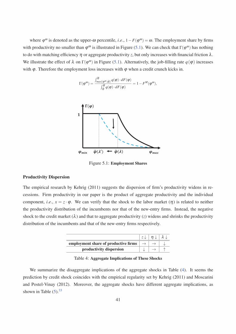
where ϕω is denoted as the upper-ω percentile, i.e., 1−F(ϕω) = ω . The employment share by firms
with productivity no smaller than ϕω is illustrated in Figure (5.1). We can check that Γ(ϕω) has nothing
to do with matching efficiency η or aggregate productivity z, but only increases with financial friction λ .
We illustrate the effect of λ on Γ(ϕω) in Figure (5.1). Alternatively, the job-filling rate q(ϕ) increases
with ϕ . Therefore the employment loss increases with ϕ when a credit crunch kicks in.
Γ(ϕω) =
´ ϕmax{ϕω ,ϕ} q(ϕ) ·dF(ϕ)´ ϕ
ϕ q(ϕ) ·dF(ϕ)= 1−FM(ϕω),
( ) ( )
( )
Figure 5.1: Employment Shares
Productivity Dispersion
The empirical research by Kehrig (2011) suggests the dispersion of firm’s productivity widens in re-
cessions. Firm productivity in our paper is the product of aggregate productivity and the individual
component, i.e., x = z ·ϕ . We can verify that the shock to the labor market (η) is related to neither
the productivity distribution of the incumbents nor that of the new-entry firms. Instead, the negative
shock to the credit market (λ ) and that to aggregate productivity (z) widens and shrinks the productivity
distribution of the incumbents and that of the new-entry firms respectively.
z ↓ η ↓ λ ↓employment share of productive firms → → ↓
productivity dispersion ↓ → ↑
Table 4: Aggregate Implications of These Shocks
We summarize the disaggregate implications of the aggregate shocks in Table (4). It seems the
prediction by credit shock coincides with the empirical regularity set by Kehrig (2011) and Moscarini
and Postel-Vinay (2012). Moreover, the aggregate shocks have different aggregate implications, as
shown in Table (5).33
41

D/K ALP T FP Y u χ RP
λ ↓ ↓ ↓ ↓ ↓ ↑ ↑ ↑z ↓ → ↓ ↓ ↓ → → ↓η ↓ → → ↓ ↓ ↑ ↓ ↑
Table 5: Aggregate Implications of These Shocks
6 Conclusion
We develop a tractable dynamic model with heterogeneous entrepreneurs to explain the interaction
between credit and labor markets. The model is used to characterize the implications of capital misallo-
cation due to credit imperfections for unemployment. The marginal value of being matched with labor
increases with an entrepreneur’s level of productivity. Therefore, high-productivity entrepreneurs offer a
higher wage in equilibrium and thus the job-filling rate increases with their productivity. A credit crunch
worsens capital misallocation by redistributing capital from high-productivity to low-productivity en-
trepreneurs. The former group of entrepreneurs is not only more productive given that capital is matched
with labor, but also they are better at being matched with labor. Consequently, a credit crunch lowers
aggregate matching efficiency in the labor market. This is the key theoretical contribution of this paper.
We then quantify the unemployment effect of credit imperfections after a calibration to the US
economy. First, the exercise on unemployment decomposition reveals that credit imperfections and the
classic labor search frictions contribute around 46% and 54%, respectively, to unemployment over the
cycles between 1951 and 2011. Secondly, we conduct a counter-factual analysis to show that the credit
crunch serves as the key driving force behind the outward shift in the Beveridge curve in the recent
recession.
Another quantitative analysis is to addresses the jobless/sluggish recovery. On the one hand, the
impulse response after VAR implies that the shock to aggregate productivity is more likely to be a cause
for the jobless or sluggish recovery in the recent three recessions. On the other hand, the shocks to the
credit and labor markets seem more responsible for the simultaneous recovery pattern between output
and unemployment in recessions prior to the 1990s. Finally, we confront the disaggregate prediction of
our model with micro-level empirical findings. Credit shocks are seemingly most essential to explain
the widening productivity distribution and the dis-proportional loss of employment in recessions.
We close with several promising directions for further research. First, as documented by Hobijn and
Sahin (2012), the outward shift in the Beveridge curve since the Great Recession occurred not only in
the US, but also in other OECD countries like Portugal, Spain, and the UK. Like Hsieh and Klenow
33As defined in Section 2, the return premium is defined as RP ≡ E [max(π (ϕ)− r, 0)]. We can rewrite it as
RP =(
τ(λ )λ
)·(
∂Y∂K
)and thus decreases with λ while increases with η and z.
42

(2007), and Restuccia, Yang and Zhu (2008), it could be interesting to initiate a cross-country analysis
for the quantitative effect of credit crunches on unemployment. Secondly, we have exclusively focused
on the effect of credit imperfections on unemployment. As shown in Section 3.4, we take a preliminary
step related to the implications of an MPS of the productivity distribution for unemployment. It may
be fruitful to combine our work with that of Bigio (2013). Thirdly, we have used a static wage contract
throughout the paper for tractability. It could be challenging but fruitful to address the same problem
with a dynamic labor contract as well as with credit imperfections and endogenous capital accumulation.
The recent progress on labor search with heterogeneity by Menzio and Shi (2010, 2011), Schaal (2012)
and Kaas and Kircher (2013) may serve as a reasonable starting point. Finally, the flexible framework of
our paper could offer a tractable tool for us to model and quantify the role of unconventional monetary
policy in curing the high rate unemployment. See the recent work by Dong and Wen (2013) for an
example.
43

References
[1] Andolfatto, David. "Business cycles and Labor-Market Search." The American Economic Review
(1996): 112-132.
[2] Azariadis, Costas, and Leo Kaas. "Capital Misallocation and Aggregate Factor Productivity."
Federal Reserve Bank of St. Louis Working Paper Series (2012).
[3] Bai, Yan, José-Víctor Ríos-Rull and Kjetil Storesletten. "Demand Shocks that Look Like Pro-
ductivity Shocks." University of Rochester, University of Minnesota and Federal Reserve Bank of
Minnesota (2012).
[4] Bethune, Zach, Guillaume Rocheteau, and Peter Rupert. "Unemployment and Household Un-
secured Debt." University of California, Santa Barbara and Irvine, mimeo (2013).
[5] Bigio, Saki. "Endogenous Liquidity and the Business Cycle." Columbia University, mimeo (2013).
[6] Berger, David. "Countercyclical Restructuring and Jobless Recoveries." Northwestern University,
mimeo (2012).
[7] Bernanke, Ben, and Mark Gertler. "Agency Costs, Net Worth, and Business Fluctuations." The
American Economic Review (1989): 14-31.
[8] Bernanke, Ben S., Mark Gertler, and Simon Gilchrist. "The Financial Accelerator in a Quanti-
tative Business Cycle Framework." Handbook of Macroeconomics 1 (1999): 1341-1393.
[9] Blanco, Julio, and Gaston Navarro. "Equilibrium Default and Slow Recoveries." NYU, mimeo
(2013).
[10] Buera, Francisco J., Joseph P. Kaboski, and Yongseok Shin. "Finance and Development: A Tale
of Two Sectors." The American Economic Review 101, no. 5 (2011): 1964-2002.
[11] Buera, Francisco J., and Benjamin Moll. "Aggregate Implications of a Credit Crunch." Princeton
and UCLA, mimeo (2013).
[12] Buera, Francisco J., Roberto Fattal-Jaef, and Yongseok Shin. "Anatomy of a Credit Crunch:
from Capital to Labor Markets." UCLA, IMF, Washington University in St. Louis and Federal
Reserve Bank of St. Louis, mimeo (2013).
[13] Carlstrom, Charles T., and Timothy S. Fuerst. "Agency costs, net worth, and business fluc-
tuations: A computable general equilibrium analysis." The American Economic Review (1997):
893-910.
44

[14] Carrillo-Tudela, Carlos, Michael Graber, and Klaus Waelde. "Unemployment and Vacancies
Dynamics with Imperfect Financial Markets." University of Essex, UCL and University of Mainz,
mimeo (2013).
[15] Chari, Varadarajan V., Patrick J. Kehoe, and Ellen R. McGrattan. "Business Cycle Account-
ing." Econometrica 75, no. 3 (2007): 781-836.
[16] Cui, Wei. "Delayed Capital Reallocation." University College London, mimeo (2013).
[17] Davis, Steven J., R. Jason Faberman, and John C. Haltiwanger. "Recruiting Intensity during
and after the Great Recession: National and Industry Evidence." No. w17782. National Bureau of
Economic Research (2012).
[18] Davis, Steven J., R. Jason Faberman, and John C. Haltiwanger. "The Establishment-Level
Behavior of Vacancies and Hiring." The Quarterly Journal of Economics 128, no. 2 (2013): 581-
622.
[19] Dong, Feng, and Yi Wen. "Unemployment under Optimal Exit Strategy." Washington University
and Federal Reserve Bank of St. Louis, work-in-progress mimeo (2013).
[20] Garin, Julio. "Borrowing Constraints, Collateral Fluctuations, and the Labor Market." University
of Georgia, mimeo (2013).
[21] Gomme, Paul, and Peter Rupert. "Theory, Measurement and Calibration of Macroeconomic
Models." Journal of Monetary Economics 54, no. 2 (2007): 460-497.
[22] Hagedorn, Marcus, Fatih Karahan, Iourii Manovskii, and Kurt Mitman. "Unemployment
benefits and unemployment in the great recession: the role of macro effects." Economics working
paper, University of Pennsylvania (2013).
[23] Hobijn, Bart, and Aysegül Sahin. "Beveridge Curve Shifts across Countries since the Great Re-
cession." Federal Bank of San Francisco Working Paper 2012-24 (2012).
[24] Holmstrom, Bengt, and Jean Tirole. "Financial intermediation, loanable funds, and the real sec-
tor." The Quarterly Journal of Economics 112, no. 3 (1997): 663-691.
[25] Hopenhayn, Hugo. "On the Measure of Distortions." UCLA, mimeo (2013).
[26] Hosios, Arthur J. "On the Efficiency of Matching and related Models of Search and Unemploy-
ment." The Review of Economic Studies 57, no. 2 (1990): 279-298.
45
[27] Hsieh, Chang-Tai, and Peter J. Klenow. "Misallocation and Manufacturing TFP in China and
India." The Quarterly Journal of Economics 124, no. 4 (2009): 1403-1448.
[28] Jaimovich, Nir, and Henry E. Siu. "The Trend is the Cycle: Job Polarization and Jobless Recov-
eries." No. w18334. National Bureau of Economic Research (2012).
[29] Jermann, Urban, and Vincenzo Quadrini. "Macroeconomic Effects of Financial Shocks." The
American Economic Review 102, no. 1 (2012): 238-271.
[30] Kaas, Leo, and Philipp Kircher. "Efficient Firm Dynamics in a Frictional Labor Market." Uni-
versity of Konstanz and University of Edinburgh, mimeo (2013).
[31] Kehrig, Matthias. "The Cyclicality of Productivity Dispersion." University of Texas at Austin,
mimeo (2011).
[32] Khan, Aubhik, and Julia K. Thomas. "Credit Shocks and Aggregate Fluctuations in an Economy
with Production Heterogeneity." Journal of Political Economy, forthcoming (2013).
[33] Kiyotaki, Nobuhiro, and John Moore. "Credit Cycles." The Journal of Political Economy 105,
no. 2 (1997): 211-248.
[34] Krusell, Per, and Anthony A. Smith, Jr. "Income and Wealth Heterogeneity in the Macroecon-
omy." Journal of Political Economy 106, no. 5 (1998): 867-896.
[35] Kurlat, Pablo. "Lemons Markets and the Transmission of Aggregate Shocks." Stanford Univer-
sity, mimeo (2012).
[36] Lagos, Ricardo. "A Model of TFP." The Review of Economic Studies 73, no. 4 (2006): 983-1007.
[37] Liu, Zheng, Jianjun Miao, and Tao Zha. "Land Prices and Unemployment." No. w19382. Na-
tional Bureau of Economic Research (2013).
[38] Liu, Zheng, and Pengfei Wang. "Credit Constraints and Self-Fulfilling Business Cycles." Ameri-
can Economic Journal: Macroeconomics, forthcoming (2011).
[39] Lucas Jr, Robert E. "On the Size Distribution of Business Firms." The Bell Journal of Economics
(1978): 508-523.
[40] Melitz, Marc J. "The Impact of Trade on Intra-Industry Reallocations and Aggregate Industry
Productivity." Econometrica 71, no. 6 (2003): 1695-1725.
[41] Menzio, Guido, and Shouyong Shi. "Block Recursive Equilibria for Stochastic Models of Search
on the Job." Journal of Economic Theory 145, no. 4 (2010): 1453-1494.
46

[42] Menzio, Guido, and Shouyong Shi. "Efficient Search on the Job and the Business Cycle." Journal
of Political Economy 119, no. 3 (2011): 468-510.
[43] Merz, Monika. "Search in the Labor Market and the Real Business Cycle." Journal of Monetary
Economics 36, no. 2 (1995): 269-300.
[44] Miao, Jianjun, Pengfei Wang, and Lifang Xu. "Stock Market Bubbles and Unemployment."
Boston University and Hong Kong University of Science and Technology, mimeo (2013).
[45] Michaillat, Pascal. "Do Matching Frictions Explain Unemployment? Not in Bad Times." The
American Economic Review 102, no. 4 (2012): 1721-1750.
[46] Moen, Espen R. "Competitive search equilibrium." Journal of Political Economy 105, no. 2
(1997): 385-411.
[47] Moll, Benjamin. "Productivity Losses from Financial Frictions: Can Self-financing Undo Capital
Misallocation?" Princeton University, mimeo (2012).
[48] Monacelli, Tommaso, Vincenzo Quadrini, and Antonella Trigari. "Financial Markets and Un-
employment." No. w17389. National Bureau of Economic Research, 2011.
[49] Moscarini, Giuseppe, and Fabien Postel-Vinay. "The Contribution of Large and Small Employ-
ers to Job Creation in Times of High and Low Unemployment." The American Economic Review
102, no. 6 (2012): 2509-2539.
[50] Mortensen, Dale T. Wage Dispersion: Why are Similar Workers Paid Differently. MIT Press
(2005).
[51] Mukoyama, Toshihiko, Christina Patterson, and Aysegül Sahin. "Job Search Behavior over the
Business Cycle." University of Virginia, Federal Reserve Board and Federal Reserve Bank of New
York, mimeo (2013).
[52] Jaimovich, Nir, and Henry E. Siu. "The Trend is the Cycle: Job Polarization and Jobless Recov-
eries." Duke and UBC, mimeo (2013).
[53] Petrongolo, Barbara, and Christopher A. Pissarides. "Looking into the Black Box: A Survey
of the Matching Function." Journal of Economic Literature 39, no. 2 (2001): 390-431.
[54] Petrosky-Nadeau, Nicolas. "TFP during a Credit Crunch." Journal of Economic Theory (2013).
[55] Petrosky-Nadeau, Nicolas, and Etienne Wasmer. "The Cyclical Volatility of Labor Markets un-
der Frictional Financial Markets." American Economic Journal: Macroeconomics 5, no. 1 (2013):
193-221.
47

[56] Pissarides, Christopher A. Equilibrium Unemployment Theory. MIT press, 2000.
[57] Restuccia, Diego, and Richard Rogerson. "Policy Distortions and Aggregate Productivity with
Heterogeneous Establishments." Review of Economic Dynamics 11, no. 4 (2008): 707-720.
[58] Restuccia, Diego, Dennis Tao Yang, and Xiaodong Zhu. "Agriculture and Aggregate Productiv-
ity: A Quantitative Cross-Country Analysis." Journal of Monetary Economics 55, no. 2 (2008):
234-250.
[59] Schaal, Edouard. "Uncertainty, Productivity and Unemployment in the Great Recession." Federal
Reserve Bank of Minneapolis, mimeo (2012).
[60] Shimer, Robert. "Contracts in a Frictional Labor Market. " MIT, mimeo (1996).
[61] Shimer, Robert. "Labor Markets and Business Cycles." Princeton University Press (2010).
[62] Wasmer, Etienne, and Philippe Weil. "The Macroeconomics of Labor and Credit Market Imper-
fections." The American Economic Review (2004): 944-963.
[63] Wang, Pengfei, and Yi Wen. "Hayashi meets Kiyotaki and Moore: A Theory of Capital Adjust-
ment Costs." Review of Economic Dynamics 15, no. 2 (2012): 207-225.
[64] Wang, Pengfei, and Yi Wen. "Financial Development and Long-Run Volatility Trends." Hong
Kong University of Science and Technology and Federal Reserve Bank of St. Louis, mimeo (2013).
[65] Wiczer, David. "Long-term Unemployment: Attached and Mismatched?." University of Min-
nesota, mimeo (2012).
[66] Williamson, Stephen D. "Financial Intermediary, Business Failures, and Real Business Cycles."
The Journal of Political Economy 95, no. 6 (1987): 1196-1216.
48

Appendix A - Data Sources, Definitions and Calculations
All the data throughout this paper are of quarterly frequency. There are three sources of data used in
Section 1 and Section 4. First, we use financial data from the Flow of Funds Accounts (FFA) to construct
the ratio of external funding over non-financial assets. We follow exactly Buera, Fattal-Jaef and Shin
(2013) for this measurement. On the one hand, the external funding corresponds to the credit market
instruments in FFA. It consists of the bank loans of the corporate and non-corporate sectors, and the
commercial papers, corporate bonds and municipal securities of the corporate business. On the other
hand, non-financial assets include real estate stock, equipment, software and inventories of the corporate
and non-financial non-corporate business.
Secondly, data on employment, unemployment rate and job creation/destruction come from Bureau
of Labor Statistics (BLS) while data on the Beveridge curve Job Opening and Labor Turnover (JOLTS).
We only consider employment by non-farm private sectors. We use unemployment rate and employment
to back out the total labor participation numbers in non-farm private sectors. The Beveridge curve with
job opening rate and unemployment rate started with the last of 2000 because that is the starting point
of the data in JOLTS.
Finally, National Income and Product Account (NIPA) documents quarterly data on output and
investment, and annual data on capital. Output is defined as the sum of private non-durable consumption
and private non-residential investment. We use the quarterly data on investment and the annual data on
capital to recover the quarterly data on capital.
49

Appendix B - A Static Simplified Model
We use a static and simplified model to illustrate the key mechanism through which credit misallocation
lowers aggregate matching efficiency. Aggregate productivity is simply set as z = 1. Each entrepreneur
has K units of net worth. The distribution of individual productivity is a simple Binomial, i.e., ϕ adopts
ϕH = μ +σ and ϕL = μ −σ with equal probability, where σ ∈ [0, μ]. As in the baseline, we model credit
and labor frictions by a collateral constraint and competitive search respectively. We first characterize
the case with only labor search frictions.
Y ∗ = max{ϕH ·m(vH , lH)+ϕL ·m(vL, lL)}
subject to
vH + vL ≤ K
lH + lL ≤ L
vi, li ≥ 0, i ∈ {L,H} ,
where vi and li denotes respectively the measure of capital and labor in sub-labor market i ∈ {L,H},
and m(·, ·) a matching technology. The efficient allocation consists of v∗H = K, v∗L = 0, l∗H = L, and l∗L = 0.
In turn, aggregate output is Y ∗ = ϕH · m(K,L), employment N∗ = m(K,L), average labor productivity
ALP∗ ≡ Y ∗N∗ = ϕH , and unemployment u∗ ≡ 1− N
L∗. Then we reach the equilibrium allocation as below.
Corollary 6. (Equilibrium Wedges under a Simple Binomial Distribution) Denote F as a Binomial
distribution such that ϕ adopts ϕH and ϕL with probability αH (λ ) and 1−αH (λ ) respectively, where
αH(λ )≡ min{
λ2, 1}
. Then
1. for i ∈ {L,H}, the total capital used by type-i entrepreneurs is
vH = min{
λ2,1
}·K, vL = K − vH .
2. aggregate output and employment is
Y = (1− τy) ·Y ∗, N = (1− τn) ·N∗,
where
1− τy = Λ(λ )≡[EF
(ϕ
1γ)]γ
ϕH=
[αH(λ )+(1−αH(λ )) ·
(ϕL
ϕH
) 1γ]γ
1− τn = Ω(λ )≡EF
(ϕ
1−γγ
)[EF
(ϕ
1γ)]1−γ =
αH(λ )+(1−αH(λ )) ·(
ϕLϕH
) 1−γγ
[αH(λ )+(1−αH(λ )) ·
(ϕLϕH
) 1γ]1−γ .
50

both of which increases with λ , decreases with σμ , lim
λ→∞τy = lim
λ→∞τn = 0, and lim
σμ →0
τy = limσμ →0
τn = 0.
Similar to Proposition 2, a credit crunch increases the wedge of output and employment. More-
over, an MPS of the productivity distribution, i.e., the increase of σμ , also lowers aggregate matching
efficiency. We use Figure 6.1 to illustrate those findings.
The main merit of using a Binomial distribution is a more clear intuition behind the transmission
mechanism from credit to labor markets. By definition, employment is N ≡ m(vH , lH) + m(vL, lL) =vH · qH + vL · qL, where qi denotes the job-filling rate in sub-labor market i. To make the analysis non-
trivial, we assume both sub-labor markets are active, i.e., vH > 0 and vL > 0. Then we have
∂N∂λ
= (qH −qL) · ∂vH
∂λ+
(vH · ∂qH
∂λ+ vL · ∂qL
∂λ
)≥ 0.
We already know that wH > wL, θH > θL, and qH > qL. Then as the above decomposition suggests,
on the one hand, the increase of λ transfers capital from low-productivity to high-productivity en-
trepreneurs, which directly implies an increase of employment. On the other hand, the increase of λmakes the use of capital more congested and thus the job-filling rate in the active sub-labor markets
decrease. However, the direct effect can be verified to dominate the indirect general-equilibrium effect.
0 0.2 0.4 0.6 0.8 10.82
0.84
0.86
0.88
0.9
0.92
0.94
0.96
0.98
1
1.02
σ/μ: Mean Preserving Spread
Ω:
End
o M
atch
ing
Eff
icie
ncy
λ=1 (Autarky)
λ=1.5
λ=∞ (Complete credit mkt)
1 1.2 1.4 1.6 1.8 20.82
0.84
0.86
0.88
0.9
0.92
0.94
0.96
0.98
1
1.02
λ: Leverage Ratio
Ω:
End
o M
atch
ing
Eff
icie
ncy
σ/μ=0
σ/μ=0.3
σ/μ=0.9
Figure 6.1: Left Panel:(
Ω, σμ
); Right Panel: (Ω,λ )
51

Appendix C - Model Extension
This section consists of three pieces of model extension.34 The first two extensions consider other
possible sources of capital misallocation. One is to introduce tax on capital revenue while the other is
to address the implications of working capital constraint. For space concern, we omit the discussion on
transition dynamics. Finally, motivated by recent empirical findings, we endogenize firm’s procyclical
recruiting effort, which in turn amplifies the transmission mechanism in our baseline.
Tax on Capital Revenue
Motivated by Restuccia and Rogerson (2008), we extend the model with a tax scheme on capital revenue
{τk (ϕ)}ϕ∈Φ.35 The expected capital revenue is then adjusted as π (ϕ) = [1− τk (ϕ)] ·π (ϕ). Meanwhile,
the active set is updated as ΦA = {ϕ| π (ϕ)≥ r} with its associated cumulative distribution as FA and the
lower bound as ϕ = in f {ΦA}. In the baseline, we characterize capital misallocation by the decrease of
the cut-off point ϕ . We generalize the notion of capital misallocation as follows.
Definition 2. Denote FA and FA′ as two pieces of productivity distribution of active entrepreneurs. FA′
causes a worse capital misallocation than FA if and only if FA Second-Order Stochastic Dominates
(SOSD) FA′ .
The employment in Equation (3.4) is now generalized by
N (FA) = EFA [q(ϕ,W )] ·K =
[ˆΦ
q(ϕ,W (FA))dFA
]·K (6.1)
where K denotes the aggregate capital supply, q(ϕ) the job-filling rate in sub-labor market ϕ and W
the expected labor revenue. As in the baseline, capital misallocation generates two competing effects
on employment. We illustrate the generalized version as below.
N (FA)−N (FA′)=
{[ˆΦ
q(ϕ,W (FA)) ·dFA −ˆ
Φq(ϕ,W (FA)) ·dFA′
]+
[ˆΦ
q(ϕ,W (FA)) ·dFA′ −ˆ
Φq(ϕ,W (FA′)) ·dFA′
]}·K.
To sharpen the analysis, we make an assumption as below, which delivers the generalized version of
the unemployment effect of capital misallocation.
Assumption 2. The distribution F is specified such that, if the truncated distribution FA SOSD FA′ ,
EFA
(ϕ
1−γγ
)[EFA
(ϕ
1γ)]1−γ >
EFA′
(ϕ
1−γγ
)[EFA′
(ϕ
1γ)]1−γ .
34For space concern, we remove all the proofs associated with this section. The proofs are available upon request.35For simplicity, we assume entrepreneurs with the same productivity share the same tax rate.
52

Corollary 7. (Wedges with Capital Revenue Tax) Under Assumption 2, if FA SOSD FA′ ,
1. the wedges to aggregate output and employment are
1− τy ≡{EFA
[(ϕ/ϕ)
1γ]}γ
∈ [0,1]
1− τn ≡EFA
(ϕ
1−γγ
)[EFA
(ϕ
1γ)]1−γ ∈ [0,1]
where (τy,τn) are larger with ΦA′ .
2. the wedges to ALP and unemployment are
1− τal p =1− τy
1− τn=
EFA
(ϕ
1γ)
EFA
[(ϕϕ
)·ϕ 1
γ] ∈ [0,1]
1+ τu = 1+ τn ·(
1−u∗
u∗
)∈ (1,∞) ,
3. the wedge to the expected wage revenue is zero while that to the interest rate is
1− τr =1− τk (ϕ)
EFA
[(ϕϕ
) 1γ] ∈ [0,1]
On the one hand, if τK (ϕ)≡ 0, then the active sets reduces to that in the baseline. On the other hand,
if τK (ϕ) is progressive, taking τK (ϕ) = α ·[
1−( ϕ−ϕ
ϕ−ϕ
) 1γ]
with α ∈ [0,1] for example, then we can check that
the active set is ΦA = {ϕ|ϕ ∈ [ϕ1, ϕ2]}, which is illustrated in Figure 6.2. Moreover, we can show that the
increase of α widens the active set ΦA and thus lowers the output and increases unemployment.
Figure 6.2: Wage Scheme with a Progressive Tax on Capital Revenue (an example)
53

Working Capital Constraint
Hosios condition is satisfied in the baseline with competitive search. Therefore the labor wedge is
zero in the baseline. However, the business cycle accounting by Chari, Kehoe and McGrattan (2007)
suggests the quantitative importance of labor wedge. This part imposes a working capital constraint
upon the baseline to produce a non-trivial labor wedge. As shown in Section 2, total wage payment
is k · θ(ϕ) ·W for entrepreneurs with productivity ϕ and with k units of capital for production. We
assume entrepreneurs have to pay part of the wage bill before production such that k ·θ(ϕ) ·W ≤ λw · k,
or equivalently,
θ(ϕ)≤ λw
W. (6.2)
In contrast to the baseline, the equilibrium wage scheme may be distorted in the presence of a
constraint on working capital. The following proposition characterizes the equilibrium wedges on pro-
ductivity, employment, interest rate, and wages, etc in the presence of the working capital constraint.
Corollary 8. (Equilibrium Wedges with Working Capital Constraint) In each period,
1. there exist pairwise cut-off values (ϕ, ϕ) such that
(a) only entrepreneurs with productivity ϕ ≥ ϕ are active in production,
(b) the wage scheme is w(ϕ) = (1− γ) ·min{ϕ, ϕ},
2. the solution to the pairwise cut-off values (ϕ, ϕ) exists and is unique, and
(a) ϕ increases with λ and has nothing to do with other variables,
(b) ϕ increases with λ , and λw,
3. the wedges to aggregate output and employment are
1− τy ≡ Λ(λ ,λw)≡E
{max
(1,(
ϕϕ
))· [min(ϕ, ϕ)]
1γ |ϕ ∈ [ϕ,ϕ]
}[E
{[min(ϕ, ϕ)]
1γ |ϕ ∈ [ϕ,ϕ]
}]1−γ·ϕ
∈ [0,1]
1− τn ≡ Ω(λ ,λw)≡E
{[min(ϕ, ϕ)]
1−γγ |ϕ ∈ [ϕ,ϕ]
}[E
{[min(ϕ, ϕ)]
1γ |ϕ ∈ [ϕ,ϕ]
}]1−γ ∈ [0,1]
and (τy,τn) decreases with λw.
54

4. the wedges to ALP and unemployment are
1− τal p =1− τy
1− τn=
E
{max
(1,(
ϕϕ
))· [min(ϕ, ϕ)]
1γ |ϕ ∈ [ϕ,ϕ]
}E
{[min(ϕ, ϕ)]
1−γγ |ϕ ∈ [ϕ,ϕ]
}·ϕ
∈ [0,1]
1+ τu = 1+ τn ·(
1−u∗
u∗
)∈ (1,∞) .
and(τal p,τu
)decreases with λw.
5. the wedges to the interest rate and to the wage are
1− τr = =1
E
{min((
ϕϕ
)1γ ,(
ϕϕ
) 1γ ·(
ϕϕ
))|ϕ ∈ [ϕ,ϕ]
} ∈ [0,1] .
1− τw =E
{[min(ϕ, ϕ)]
1γ |ϕ ∈ [ϕ,ϕ]
}E
{max
(1,(
ϕϕ
))· [min(ϕ, ϕ)]
1γ |ϕ ∈ [ϕ,ϕ]
} ∈ [0,1] .
and (τr,τw) decreases with λw.
If λw is high enough, then ϕ > ϕ and we are back to the baseline model. Otherwise, as indicated
in the above corollary, the optimal wage scheme becomes flattened for ϕ ∈ [ϕ, ϕ]. The wage scheme
with a binding working capital constraint provides a micro foundation for equilibrium wage rigidity,
i.e., entrepreneurs choose not to adjust their wage scheme if their productivity ϕ ∈ [ϕ, ϕ]. We illustrate
it in Figure 6.3.
( , ( ) )
( )( )
Figure 6.3: Wage Scheme with Working Capital Constraint
The possibility of non-trivial labor wedge is the main insight gained from the working capital con-
straint. The marginal value of being matched with labor increases with entrepreneur’s productivity.
Thus wage scheme and job-filling rate increase with productivity. However, due to the working capital
constraint, high-productivity entrepreneurs would have to cut down the otherwise high wage, which in
turn lowers employment and labor expenditure.
55

Endogenous Recruiting Effort
The recent empirical findings by Davis, Faberman and Haltiwanger (2012) suggest that, in addition to
posting vacancies, firm’s recruiting effort also includes “increase advertising or search intensity per va-
cancy, screen applicants more quickly, relax hiring standards, improve working conditions, and offer
more attractive compensation to prospective employees”.36 Furthermore, they show that firm’s recruit-
ing effort is procyclical. To this end, we follow Pissarides (2000) and Bai, Ríos-Rull and Storesletten
(2012) to endogenize firm’s search effort.
For simplicity, we assume firm’s search effort is made after observing the aggregate state variable,
but before the realization of their own productivity level. Entrepreneurs use worker’s labor input to
increase their own search effort s, which may include advertising and screening effort.37 More specif-
ically, σ ∈ (0,1) of capital revenue is pledgeable to workers. Matching function is m(v(ϕ)e(s) , l (ϕ)),where s denotes the average recruiting effort. Each entrepreneur treats s as given. In equilibrium, we
have s = s. Denote the modified market tightness as θ (ϕ)≡ l(ϕ)v(ϕ)e(s) . The job-filling rate and job finding
rate are modified as below.
q(θ (ϕ) ,s) =m(v(ϕ)e(s) , l (ϕ))
v(ϕ)e(s)· e(s) = m(1,θ (ϕ)) · e(s)
p(θ (ϕ) ,s) =m(v(ϕ)e(s) , l (ϕ))
l(ϕ)= m
(1
θ (ϕ),1
)=
q(θ (ϕ) ,s)θ (ϕ) · e(s) .
Corollary 9. In equilibrium s = s. Moreover, given s, aggregate output and unemployment is adjusted
as
Y = z ·Λ(λ ) ·m(e(s) ·K,L)
u = 1−Ω(λ ) ·m(
e(s) ·KL
,1
),
and the aggregate matching efficiency is η = Ω(λ ) ·η · e(s).It remains for us to characterize the choice of recruiting effort s. First, given (s,s), the decision by
active entrepreneur-(a,ϕ) is formulated as below.
π (ϕ,s)≡ maxs.t. p(θ(ϕ),s)·w(ϕ)=W
{q(θ (ϕ) ,s) · (ϕ −w(ϕ))}
The modified market tightness θ(ϕ) is pinned down by the FOC ∂m(θ(ϕ),1)∂θ(ϕ) = W
ϕ . Secondly, given s,
the individual decision rule on lending or borrowing depends on ϕ(s), where π(ϕ(s),s) = r. Therefore s
is determined by
max {(1−σ) · {λ [1−F(ϕ(s))] ·E [(π(ϕ,s)− r) |ϕ ≥ ϕ(s)]+ r}− c(s)} ,36The recent work by Mukoyama, Patterson and Sahin (2013) complements to Davis, Faberman and Haltiwanger (2012)
by focusing on the job search intensity of worker side. Our paper focuses on the endogenous search effort by the firm side.37We also tried an alternative setup to endogenize firm’s recruiting effort. It is the entrepreneurs who incur non-pecuniary
disutility for recruiting effort. The alternative extension is available upon request.
56

where λ [1−F(ϕ(s))]E [(π(ϕ,s)− r) |ϕ ≥ ϕ(s)]+ r denotes the expected capital revenue with search
effort s by workers, and σ proportion can be pledgeable to them, and c(s) denotes the effort cost. We
assume e(0) = sL > 0. That is, if none of the entrepreneurs exert positive search effort, we are back to the
baseline model. Besides, we assume e′ (s)> 0, e′′ (s)< 0, c(0) = 0, c′ (s)> 0, and c′′ (s)≥ 0. FOC upon the
above equation delivers the endogenous choice of recruiting effort. First, the equilibrium search effort s
increases with (z,η ,λ ). That is, these shocks will be amplified through the search effort. In particular,
since η = Ω(λ ) ·η · e(s(z,λ ,η)), the decrease of either λ or η lowers aggregate matching efficiency in
both direct and indirect way. We illustrate the amplification in Figure (6.4).
( ) ( )
( )
Figure 6.4: Unemployment Effect of Capital Reallocation with Endogenous Recruiting Effort
57

Appendix D - Proofs
Proof on Proposition 1
Proof. Substituting the participation constraint p(θ(ϕ))w(ϕ) =W into the objective function and using the fact
that p(θ(ϕ)) = q(θ(ϕ))θ(ϕ) yields
π(ϕ,W ) = max {q(θ(ϕ))ϕ −θ(ϕ)W} ,
and thus the FOC is q′(θ(ϕ)) = Wϕ , which pins down the market tightness θ(ϕ) in active submarket-ϕ ∈ ΦA.
Using Implicit Function Theorem and the concavity of q(·) suggests that θ(ϕ) increases with ϕ and decreases
with W . In turn, we recovery the wage scheme as w(ϕ) = Wp(θ(ϕ)) . Since p(θ(ϕ)) decreases with θ(ϕ), we know
that w(ϕ) increases with ϕ . Finally, using Envelope Theorem reveals that π(ϕ,W ) increases with ϕ and decreases
with W .
Proof on Lemma 1
Proof. The net revenue by entrepreneur-(a,ϕ) is
maxk∈[0,λ ·a]
{π(ϕ,W ) · k− r · (k−a)+(1−δ ) ·a},
where π(ϕ,W ) ·k denotes the capital revenue and b = k−a is the debt if positive and the loan if negative. The
above problem can be rewritten as maxk∈[0,λ ·a]
[π(ϕ,W )− r] ·k+[r+(1−δ )] ·a. Since the net revenue is linear k, and
k ∈ [0,λ · a], only corner solutions, i.e., k = λa or k = 0, will be considered. On the one hand, if π(ϕ,W ) > r,
the entrepreneurs not only want to engage in production, but also want to borrow as much as they can. On the
other hand, if π(ϕ,W )< r, then the entrepreneurs prefer to lending to others. Since π(ϕ,W ) increases with ϕ , if
we define the cut-off point ϕ as π(ϕ,W ) = r, then entrepreneurs choose to be active in production with a binding
borrowing constraint if and only if ϕ > ϕ .
Proof on Corollary 1
Proof. First, as shown in Lemma 1, the active set is ΦA ≡ {ϕ|ϕ ∈ [ϕ,ϕ]} = {ϕi|ϕi ∈ [ϕi,ϕ i]}. Therefore, thetruncated distribution of productivity by active entrepreneurs is
FA(ϕ) =ˆ ϕ
ϕf (ϕ|ϕ ≥ ϕ)dϕ =
F(ϕ)−F(ϕ)1−F(ϕ)
.
Secondly, according to Proposition 1 and Lemma 1, wage scheme w(ϕ) increases with ϕ and entrepreneurswith higher individual productivity, q(ϕ), is more likely to be matched with workers. Therefore, the productivitydistribution of finally matched capital is
FM(ϕ) =
´ ∞0
´ ϕϕ k(ϕ ′,a) ·q(ϕ ′) ·h(ϕ,a)dϕda´ ϕ
ϕ k(ϕ ′,a) ·q(ϕ ′) ·dF(ϕ ′)=
´ ϕϕ q(ϕ ′) ·dF(ϕ ′)´ ϕϕ q(ϕ ′) ·dF(ϕ ′)
.
58

Finally, we use the following lemma to prove FM(ϕ)< FA(ϕ)< F(ϕ).Lemma 3. Assume ε(ϕ)> 0 for ϕ ∈ [ϕ,ϕ]. Given any ϕ ∈ [ϕ,ϕ], define
F1 (ϕ) ≡´ ϕ
ϕ ε(ϕ ′)dϕ ′´ ϕ
ϕ ε(ϕ ′)dϕ ′ , F2 (ϕ)≡´ ϕ
ϕ ε(ϕ ′)ϑ(ϕ ′)dϕ ′´ ϕ
ϕ ε(ϕ ′)ϑ(ϕ ′)dϕ ′ ,
where ϑ(ϕ) increases with ϕ and is bounded by [0,1]. Then F1 (ϕ)≤ F2 (ϕ).We leave the proof of this lemma at the end of this part. Now use this lemma to prove FM (ϕ) < FA (ϕ) <
F (ϕ) . First, we can rewrite FA (ϕ) and FM (ϕ) as below.
FA (ϕ) =
´ ϕϕ f (ϕ ′)dϕ ′´ ϕ
ϕ f (ϕ ′)dϕ ′ , FM (ϕ) =
´ ϕϕ f (ϕ ′)q(ϕ ′)dϕ ′´ ϕ
ϕ f (ϕ ′)q(ϕ ′)dϕ ′ .
Therefore, if we treat ε (ϕ) as f (ϕ), and ϑ (ϕ) as q(ϕ), which has been proved to increase with ϕ in Propo-sition 1, then using the above lemma immediately suggests FM (ϕ) ≤ FA (ϕ), i.e., FM(ϕ) first-order stochasticdominates (FOSD) FA (ϕ). Moreover, we can rewrite FA (ϕ) as below.
FA (ϕ) =
´ ϕϕ f (ϕ ′) ·1{ϕ ′≥ϕ}dϕ ′´ ϕ
ϕ f (ϕ ′) ·1{ϕ ′≥ϕ}dϕ ′ .
If we treat ϑ(ϕ) as 1{ϕ≥ϕ}, which increases with ϕ and bounded by [0,1] in this scenario, then immediately
the above lemma implies FA(ϕ) ≤ F(ϕ). We close this part by proving the aforementioned lemma. DefineF3 (ϕ)≡ F2 (ϕ)−F1 (ϕ). Then we have
F ′3(ϕ) = F ′
2 (ϕ)−F ′1 (ϕ)
=ε(ϕ)ϑ(ϕ)´ ϕ
ϕ ε(ϕ ′)ϑ(ϕ ′)dϕ ′ −ε(ϕ)´ ϕ
ϕ ε(ϕ ′)dϕ ′
= ε(ϕ)
[ϑ(ϕ)
´ ϕϕ ε(ϕ ′)dϕ ′ −´ ϕ
ϕ ε(ϕ ′)ϑ(ϕ ′)dϕ ′]· ε(ϕ)[´ ϕ
ϕ ε(ϕ ′)ϑ(ϕ ′)dϕ ′]·[´ ϕ
ϕ ε(ϕ ′)dϕ ′] .
Now we define F4 (ϕ) ≡ ϑ(ϕ)´ ϕ
ϕ ε(ϕ ′)dϕ ′ − ´ ϕϕ ε(ϕ ′)ϑ(ϕ ′)dϕ ′. Then we immediately know that, since
ϑ(ϕ) is an increasing function in ϕ , so is F4 (ϕ). Moreover, notice that F4 (ϕ)< 0 and F4 (ϕ)> 0, and thus thereexists a cut-off ϕ ∈ (ϕ,ϕ)such that F4 (ϕ) < 0 when ϕ ∈ (ϕ, ϕ) and F4 (ϕ) > 0 when ϕ ∈ (ϕ,ϕ). In turn, weknow that,
F ′3 (ϕ)
⎧⎨⎩< 0 i f ϕ ∈ (ϕ, ϕ)
> 0 i f ϕ ∈ (ϕ,ϕ) .
Besides, since F3 (ϕ) = F3 (ϕ) = 0, we know that F3 (ϕ)≡ F2 (ϕ)−F1 (ϕ)≤ 0 is always satisfied.
Proof on Corollary 2
Proof. First, using the result on capital demand mentioned above, the constrained optimization by entrepreneur-
(a,ϕ) can be rewritten as
V (a,ϕ;X) = max{
log(c)+β ·E[V (a′,ϕ ′;X ′) |X]} ,subject to c+a′ =Ψ(ϕ) ·a, where Ψ(ϕ) =max{π(ϕ)− r, 0}·λ +[r+(1−δ )]. Then we substitute the capital de-
59

mand of Lemma 1 into the budget constraint and thus reach the simplified version of the constrained optimization
problem by entrepreneur-(a,ϕ).Secondly, we address the policy function. Guess the value function is linear with own net worth, i.e., V (a,ϕ)=
C(ϕ)+D · log(a), then we have
V (a,ϕ) =C(ϕ)+D · log(a) = maxa′∈(0,Ψ(ϕ)·a)
{log(Ψ(ϕ) ·a−a′)+β ·E[C(ϕ ′)+D · log(a′)|ϕ]} ,
where Ψ(ϕ) = max{π(ϕ)− r, 0} ·λ +[r+(1−δ )] . FOC suggests a′ =(
βD1+βD
)·Ψ(ϕ) ·a. In turn, the above
Bellman equation can be rewritten as
C(ϕ)+D · log(a) = log[(
1
1+βD
)·Ψ(ϕ) ·a
]+β ·
{E[C(ϕ ′)|ϕ]+D · log
[(βD
1+βD
)·Ψ(ϕ) ·a
]}.
Therefore D = 11−β , and thus a′ = β ·Ψ(ϕ) ·a. In turn, d = Ψ(ϕ) ·a−a′ = (1−β ) ·Ψ(ϕ) ·a.
Proof on Lemma 2
Proof. Denote Φ∗ as the efficient set of active capital and labor, i.e., Φ∗ = {ϕ| l(ϕ)> 0, v(ϕ)> 0}. Assume themeasure of Φ∗ contains at least two types of productivity ϕ , then for ϕi ∈ Φ∗, the FOC suggests
ϕi ·mv(v(ϕi), l(ϕi)) = μK
ϕi ·ml(v(ϕi), l(ϕi)) = μL,
where μK and μL denotes the Lagrangian multiplier of the constraints on capital and labor respectively. Thenwe have
mv(v(ϕi), l(ϕi))
ml(v(ϕi), l(ϕi))=
mv(1,θ(ϕi))
ml(1,θ(ϕi))=
μK
μL,
where the first equation uses the fact that mv and ml are homogeneous of degree one. Immediately we knowθ(ϕi) is constant for ϕi ∈ Φ∗. Then we know that
ϕi ·mv(,θ(ϕi)) = μK .
Therefore ϕi is unique and is determined by μK and μL. Thus there is only one element in Φ∗. It then goeswithout say that Φ∗ = {ϕ}. In turn,
Y ∗ =ˆ
Φϕm(v∗(ϕ), l∗(ϕ))dϕ = ϕ ·m(K,L).
Proof on Proposition 2
Proof. First, the clearing condition could be further simplified as λ · [1−F (ϕ)] = 1. Using Implicit Function
Theorem immediately suggests that ϕ increases with λ , and limλ→1
ϕ = ϕ and limλ→∞
ϕ = ϕ .
Secondly, The aggregate output is defined as Y =´ ∞
0
´ ϕϕ ϕv(ϕ,a)q(ϕ)dϕda. Since v(ϕ,a) = k(ϕ,a)h(ϕ,a) =
60

λa f (ϕ)g(a) ·1ϕ∈ΦA , the output can be rewritten as
Y =
[ˆ ϕ
ϕϕ ·q(ϕ) ·dF(ϕ)
]·λK.
When the matching function in sub-labor market ϕ is m(l(ϕ),v(ϕ)) = η · l(ϕ)1−γv(ϕ)γ , then the matching
probability by entrepreneur-ϕ is q(ϕ) = m(l(ϕ),v(ϕ))v(ϕ) = η · θ(ϕ)1−γ . In turn, the FOC is simplified as q′(ϕ) =
η · (1− γ) ·θ(ϕ)−γ = Wϕ , and thus θ(ϕ,W ) =
[η(1−γ)ϕ
W
]1γ . As a result, we have
q(ϕ,W ) = η ·[
η(1− γ)W
]1−γ
γ ·ϕ1−γ
γ
p(ϕ,W ) =W
(1− γ) ·ϕπ(ϕ,W ) = η
1γ γ(1− γ)
1γ −1W 1− 1
γ ·ϕ 1γ
and thus, for ϕ ∈ ΦA, the optimal wage scheme is as w(ϕ,W ) = Wp(ϕ,W ) = (1− γ) ·ϕ . Moreover, the labor
resource constraint can be rewritten as
λKˆ ϕ
ϕθ(ϕ ,W )dF(ϕ) =
[η(1− γ)
W
]1γ ·K ·
[λˆ ϕ
ϕϕ
1γ dF(ϕ)
]= L.
Since λ´ ϕ
ϕ ϕ1γ dF(ϕ) = λ [1−F(ϕ)] ·
( ´ ϕϕ ϕ
1γ dF(ϕ)
1−F(ϕ)
)= EF
(ϕ
1γ |ϕ ∈ [ϕ,ϕ]
), we have
[η(1− γ)
W
]1γ =
L
K ·EF
(ϕ
1γ |ϕ ∈ [ϕ,ϕ]
) .
Therefore the aggregate output can be further rewritten.
Y =
ˆ ˆ ϕmax
ϕz ·ϕv(ϕ)q(ϕ)dϕdG(a).
= zη ·[
η(1− γ)W
]1−γ
γ ·K[
λˆ ϕmax
ϕϕ
1γ dF(ϕ)
]=
{zη(EF
(ϕ
1γ |ϕ ∈ [ϕ,ϕ]
))γ}·Kγ L1−γ
= z ·(EF
(ϕ
1γ |ϕ ∈ [ϕ,ϕ]
))γ·m(K,L).
which can be immediately verified by using change of variables. Then equilibrium TFP is obtained as below.
T FP ≡ YKγ L1−γ = z ·η ·
(E
(ϕ
1γ |ϕ ∈ [ϕ,ϕ]
))γ.
Now we characterize unemployment. By definition, the total matched labor (and capital) can be formulated
as below.
N ≡ˆ ∞
0
ˆ ϕ
ϕv(ϕ,a)q(ϕ)dϕda =
[ˆ ϕ
ϕq(ϕ) ·dF(ϕ)
]·λK = N = EF [q(ϕ)|ϕ ≥ ϕ] ·K.
Moreover, we have
61

N ≡[ˆ ϕ
ϕq(ϕ) ·dF(ϕ)
]·λK =
[ηˆ ϕ
ϕ
[η(1− γ)ϕ
W
]1−γ
γ ·dF(ϕ)
]·λK
= η
(ˆ ϕ
ϕϕ
1−γγ ·dF(ϕ)
)⎡⎢⎣ L
K ·EF
(ϕ
1γ |ϕ ∈ [ϕ,ϕ]
)⎤⎥⎦
1−γ
λK = Ω(λ ) ·m(K,L),
where Ω(λ ) ≡EF
(ϕ
1−γγ |ϕ∈[ϕ ,ϕ]
)[EF
(ϕ
1γ |ϕ∈[ϕ,ϕ]
)]1−γ . Since γ ∈ (0,1), Jensen’s inequality suggests EF
(ϕ
1−γγ |ϕ ∈ [ϕ,ϕ]
)<
[EF
(ϕ
1γ |ϕ ∈ [ϕ,ϕ]
)]1−γand thus N < m(K,L) = N∗. Consequently, unemployment is
u ≡ 1− NL= 1−
⎧⎪⎪⎨⎪⎪⎩EF
(ϕ
1−γγ |ϕ ∈ [ϕ,ϕ]
)[EF
(ϕ
1γ |ϕ ∈ [ϕ,ϕ]
)]1−γ .
⎫⎪⎪⎬⎪⎪⎭ ·η ·(
KL
)γ.
Therefore, u decreases with η , but has nothing to do with z.
Now we address the factor price in labor and credit markets in turn. On the one hand,[
η(1−γ)W
]1γ = L
K·EF
(ϕ
1γ |ϕ∈[ϕ,ϕ]
) ,
we know that
W = η(1− γ)[(
KL
)·EF
(ϕ
1γ |ϕ ∈ [ϕ,ϕ]
)]γ.
On the other hand, we already prove that
Y =
{η(EF
(ϕ
1γ |ϕ ∈ [ϕ,ϕ]
))γ}·Kγ L1−γ .
Immediately we have W = ∂Y∂L . Then we need to pin down the interest rate in the credit market. Since
π(ϕ,W ) = r and
π(ϕ,W ) = q(ϕ,W )(ϕ −w(ϕ)) = η (θ(ϕ,W ))1−γ γϕ,
the market tightness can be rewritten as θ(ϕ,W ) =(
rηγϕ
) 11−γ ·(
ϕϕ
) 1γ. In turn, the labor resource constraint
can be re-formulated as
λK(
rηγϕ
) 11−γ
·ˆ ϕ
ϕ
(ϕϕ
) 1γ
dF(ϕ) = L.
Therefore, the interest rate can be rewritten as
r∂Y/∂K
=ϕ
1γ
EF
(ϕ
1γ |ϕ ∈ [ϕ,ϕ]
) =ϕ
1γ
i
EFi
(ϕ
1γ
i |ϕi ∈ [ϕi,ϕ i]
) ≡ 1− τK .
Since EF
[(ϕϕ
) 1γ |ϕ ∈ [ϕ,ϕ]
]decreases ϕ and ϕ increases with λ , we know that r
∂Y/∂K = 1
EF
[(ϕϕ
) 1γ |ϕ∈[ϕ,ϕ]
] ,
62

which increases with λ . Moreover, we have
limλ→∞
r∂Y/∂K
= limα→0
r∂Y/∂K
= 1, limϕ i→∞
r∂Y/∂K
= 1− αγ.
Finally, we show why Ω(λ ) increases with λ . It is immediately done by using Assumption 1. Furthermore,
we make further characterization on Ω(λ ). Notice that we can rewrite Ω(λ ) as Ω(λ ) =λ γ ·´ ϕ
ϕ ϕ1−γ
γ dF(ϕ)[´ ϕϕ ϕ
1γ dF(ϕ)
]1−γ . Denote
A(λ ) =´ ϕ
ϕ ϕ1−γ
γ dF(ϕ) and B(λ ) =´ ϕ
ϕ ϕ1γ dF(ϕ), then after some algebraic manipulation, we have
Ω′(λ ) =λ γ
B(λ )1−γ
{( γλ
)A(λ )+A′(λ )
[1− (1− γ)
(A(λ )B(λ )
)ϕ(λ )
]},
where
A′(λ ) =−(ϕ(λ ))1−γ
γ · f (ϕ(λ )) · ϕ ′(λ ) =−(ϕ(λ ))1−γ
γ · f (ϕ(λ )) ·[
1
λ 2· 1
f (ϕ)
]=−(ϕ(λ ))
1−γγ ·(
1
λ 2
).
Therefore, Ω′(λ )> 0 if and only if
( γλ
)A(λ )+A′(λ )
[1− (1− γ)
(A(λ )B(λ )
)ϕ(λ )
]=
(1
λ
)⎧⎪⎨⎪⎩γˆ ϕ
ϕϕ
1−γγ dF(ϕ)−
(1
λ
)(ϕ(λ ))
1−γγ
⎡⎢⎣1− (1− γ)
⎛⎜⎝´ ϕ
ϕ ϕ1−γ
γ dF(ϕ)´ ϕ
ϕ ϕ1γ dF(ϕ)
⎞⎟⎠ ϕ(λ )
⎤⎥⎦⎫⎪⎬⎪⎭> 0,
or, equivalently, Ω′(λ )> 0 if and only if
γ >
(1
λ
)·
⎡⎢⎣ (ϕ(λ ))1−γ
γ
´ ϕϕ ϕ
1−γγ dF(ϕ)
⎤⎥⎦ ·⎡⎢⎣1− (1− γ)
⎛⎜⎝´ ϕ
ϕ ϕ1−γ
γ dF(ϕ)´ ϕ
ϕ ϕ1γ dF(ϕ)
⎞⎟⎠ ϕ(λ )
⎤⎥⎦ .
Notice that(
1λ)< 1,
(ϕ(λ ))1−γ
γ
´ ϕϕ ϕ
1−γγ dF(ϕ)
< 1 while 1− (1− γ)
( ´ ϕϕ ϕ
1−γγ dF(ϕ)
´ ϕϕ ϕ
1γ dF(ϕ)
)ϕ(λ ) > γ , thus we might use some
famous inequality to make sure the product of several items of the right-hand-side is smaller than γ , if that would
be true.
(1
λ
)·
⎡⎢⎣ (ϕ(λ ))1−γ
γ
´ ϕϕ ϕ
1−γγ dF(ϕ)
⎤⎥⎦ ·⎡⎢⎣1− (1− γ)
⎛⎜⎝´ ϕ
ϕ ϕ1−γ
γ dF(ϕ)´ ϕ
ϕ ϕ1γ dF(ϕ)
⎞⎟⎠ ϕ(λ )
⎤⎥⎦ =
(1
λ
)·
⎧⎪⎨⎪⎩ (ϕ(λ ))1−γ
γ
´ ϕϕ ϕ
1−γγ dF(ϕ)
− (1− γ) · (ϕ(λ ))1γ
´ ϕϕ ϕ
1γ dF(ϕ)
⎫⎪⎬⎪⎭=
(1
λ
)·
⎧⎪⎪⎨⎪⎪⎩1
´ ϕϕ
(ϕ
ϕ(λ )
) 1−γγ
dF(ϕ)− 1− γ´ ϕ
ϕ
(ϕ
ϕ(λ )
) 1γ
dF(ϕ)
⎫⎪⎪⎬⎪⎪⎭ .
Ω′(λ )> 0, or Assumption 1 is held if and only if
EF
[(ϕϕ
) 1γ|ϕ ∈ (ϕ,ϕ)
]·{
1−(
1
γ
)·[
1−F (ϕ)ϕ · f (ϕ)
]}≤ 1.
63

Proof on Corollary 3
Proof. There are at least two ways to prove this result. On the the one hand, we can verify this claim by the follow-ing reasoning. Since we’ve proved that the optimal wage scheme in active sub-labor markets is w(ϕ) = (1− γ)ϕ ,we know that all active entrepreneurs gets γ proportion of realized output. Then by definition, the aggregateaccumulated wealth by entrepreneurs,
{´Ψ(ϕ)dF(ϕ)
} ·K, should equal to the capital stock after depreciation,(1−δ ) ·K, plus γ proportion of the aggregate output, γY . On the other hand, we can prove the result by straight-forward calculation as below. As defined in the context, Ψ(ϕ) = λ ·max{π(ϕ)− r,0}+ r+(1− δ ). Then wehave
ˆΨ(ϕ)dF(ϕ) =
ˆ[λ ·max{π(ϕ)− r,0}+ r+(1−δ )]dF(ϕ)
= λ ·ˆ
max{π(ϕ)− r,0}dF(ϕ)+ r+(1−δ )
=
{λ ·ˆ ϕ
ϕ
[(ϕϕ
) 1γ−1
]+1
}· r+(1−δ ).
Then using the clearing condition in credit market, i.e., λ = 1/ [1−F(ϕ)], then we have
{ˆΨ(ϕ)dF(ϕ)
}·K =
{λ ·ˆ ϕ
ϕ
[(ϕϕ
) 1γ−1
]+1
}· rK +(1−δ )K
=
{EF
[(ϕϕ
) 1γ−1|ϕ ∈ [ϕ,ϕ ]
]+1
}· (1− τ) ·
(∂Y∂K
·K)+(1−δ )K
= γY +(1−δ )K.
Therefore the aggregate transition dynamics is obtained as below.
Kt+1 = β ·[ˆ
ΦΨt(ϕ)dFt(ϕ)
]·Kt = β · [γYt +(1−δ )Kt ] .
Proof on Proposition 3
Proof. Given w, the active entrepreneur’s decision is
π(ϕ) · k = maxl
{ηϕkγ l1−γ −wl
}.
FOC suggests l = (ηϕ)1γ(
1−αw
) 1γ k, which in turn implies
π(ϕ) = γ (ηϕ)1γ
(1−α
w
) 1−γγ
.
Since π(ϕ) increases with ϕ , the cut-off point ϕ is determined by π(ϕ,w) = r. The capital and labor demand
64

then is obtained as below.
k(ϕ,a) =
⎧⎨⎩λ ·a i f ϕ ≥ ϕ
0 i f ϕ < ϕ
l(ϕ,a) = (ηϕ)1γ
(1−α
w
) 1γ
k(ϕ,a).
In turn, the clearing conditions in credit market,´ ∞
0
´ ϕϕ k(ϕ,a)h(ϕ,a)dϕda=K, can be simplified as λ · [1−F(ϕ)] =
1. Meanwhile, the resource constraint in the labor market,´ ∞
0
´ ϕϕ l(ϕ,a)h(ϕ,a)dϕda = L, can be rewritten as below.
[η(1−α)
w
] 1γ(
λKˆ ϕ
ϕϕ
1γ dF(ϕ)
)= L.
Since λ · [1−F(ϕ)] = 1, we have λ´ ϕ
ϕ ϕ1γ dF(ϕ)=EF
(ϕ
1γ |ϕ ∈ [ϕ,ϕ]
), and therefore
[η(1−α)
w
] 1γ= L
K·EF
(ϕ
1γ |ϕ∈[ϕ,ϕ]
) .By definition, aggregate output is
Y =
ˆ ∞
0
ˆ ϕ
ϕy(ϕ,a)h(ϕ,a)dϕda
=
ˆ ∞
0
ˆ ϕ
ϕ
(π(ϕ,w)k(ϕ,a)
γ
)h(ϕ,a)dϕda
=
[η(1−α)
w
] 1−γγ(
λKˆ ϕ
ϕϕ
1γ dF(ϕ)
)
=
{η(EF
(ϕ
1γ |ϕ ∈ [ϕ,ϕ]
))γ}·Kγ L1−γ ,
and thus T FP ≡ YKγ L1−γ = ηz
(EF
(ϕ
1γ |ϕ ∈ [ϕ,ϕ]
))γ.
Proof on Corollary 4
Proof. By definition, we have
lt − lt+1 = kt(ϕt ,at)qt(ϕt)−E [kt+1(ϕt+1,at+1) ·qt+1(ϕt+1)]
= λt at ·1{ϕt≥ϕt}qt(ϕt)−Eϕt+1
[λt+1at+1 ·1{ϕt+1≥ϕt+1}qt+1(ϕt+1)
]= λt at ·1{ϕt≥ϕt}qt(ϕt)−λt+1at+1
[ρ ·1{ϕt≥ϕt+1}qt+1(ϕt)+(1−ρ) ·
ˆΦ
1{ϕ≥ϕt+1}qt+1(ϕ) ·dF(ϕ)]
= at ·{
λt ·1{ϕt≥ϕt}qt(ϕt)−λt+1βΨ(ϕt) ·[
ρ ·1{ϕt≥ϕt}qt+1(ϕt)+(1−ρ) ·ˆ
Φ1{ϕ≥ϕt+1}qt+1(ϕ) ·dF(ϕ)
]}≡ at ·Δt,t+1(ϕ t).
Proof on Corollary 5
Proof. The first part is obvious. When it comes to growth rate, by definition and using the results of the first part,
65

we have
E
[kt+1
kt|(kt ,ϕt ;Xt)
]= β ·
(Ψt(ϕt)
λt
)·E[1{ϕ ′≥ϕ(X ′)} ·λt+1|(ϕt ,Xt)
]= β ·
(Ψt(ϕt)
λt
)·E{[
ρ ·1{ϕt≥ϕt+1}+(1−ρ) · (1−F (ϕt+1))]·λt+1|(ϕt ,Xt)
}.
Meanwhile,
E
[nt+1
nt|(nt ,ϕt ;Xt)
]=
E[kt(ϕ ′
t+1,at+1)qt+1(ϕ ′t+1)]
kt(ϕt ,at)qt(ϕt)
= β ·Ψt(ϕt)
(λt+1
λt
)⎡⎣ρ ·(
qt+1(ϕt)
qt(ϕt)
)+(1−ρ) ·
⎛⎝´ ϕϕt+1
q(ϕt+1)dF(ϕt+1)
qt(ϕt)
⎞⎠⎤⎦ .
66