Embed Size (px)
Citation preview

Economic Development and the Organization ofProduction
Nicolas Roys and Ananth Seshadri⇤
University of Wisconsin Madison
October 27, 2014
Abstract
We present a heterogeneous agent model with occupational choice and endogenous
accumulation of skills to examine the organization of production both within and across
countries. Quality and quantity of workers are imperfect substitutes. The span of con-
trol is endogenously determined by the quality of workers assigned to an entrepreneur.
We calibrate the model to match certain features of the US economy. It yields a number
of empirical implications for firm heterogeneity, occupational choice and the life cycle
dynamics of firm size and earnings. Varying the aggregate efficiency of economies, we
find that entrepreneur and worker human capital can substantially improve our under-
standing of various empirical regularities pertaining to the organization of production
across countries.
Keywords: sorting, occupational choice, human capital, development
⇤We have benefited from conversations with Ufuk Akcigit, Paco Buera, Dean Corbae, Steven Durlauf,Rasmus Lentz, Dale Mortensen, Vincenzo Quadrini, Diego Restuccia, Andrés Rodríguez-Clare, Juan Sanchez,Lones Smith and Robert Townsend.
1
1 Introduction
Economists have long been interested in the sources of per capita income differences acrosscountries. The relative importance of aggregate factor inputs and technology differences hasbeen subject of considerable scrutiny. A recent growing literature, based on the work ofLucas (1978) and Hopenhayn (1992), investigates whether the allocation of resources inputsacross firms can matter for aggregate outcomes.1 Poorer countries are characterized by largermicroeconomic gaps as documented by Banerjee and Duflo (2005), Restuccia and Rogerson(2008) and Hsieh and Klenow (2009). While there exists a body of work that analyzes theallocation of physical capital across firms as well as the importance of financial markets,2
much less is known about the allocation of human capital. A robust empirical finding isthat larger firms have persistently higher average products of labor and capital. We takethe view that a firm is persistently more productive and large partly because its workforceis composed of highly skilled employees that allow an entrepreneur to spread his skills overa large scale. How is production by individuals with heterogeneous skills organized acrossfirms within a country? Are aggregate factors affecting the organization of production?
The lack of firm growth and the large number of less productive, small firms in developingcountries are well documented.3 What is the role of human capital and skills investmentfor understanding these patterns? Human capital is not directly observable. Yet, severalpieces of evidence suggest that it matters for firms’ outcomes. In many surveys, the relativescarcity of skills is mentioned as a primary obstacle for the growth of firms. In the WorldBank Enterprises Surveys, an “inadequately educated workforce” is considered to be oneof the main obstacles to conduct business. Using these same data, Gennaioli et al. (2013)find that entrepreneurial schooling is fundamental for understanding productivity differencesacross firms and conjecture that entrepreneurial human capital may play a central role indetermining firm productivity. Bloom et al. (2013) find that management quality is stronglycorrelated with firm-level productivity and that the education of both managers and non-managers is associated with better management scores.
Motivated by the empirical evidence, we build a model of acquisition and allocation of hu-man capital across firms and we distinguish between worker human capital and entrepreneurhuman capital. In the seminal occupational choice model of Lucas (1978), the most talented
1See the survey by Hopenhayn (2014).2See for instance Quadrini (2000); Cagetti and De Nardi (2006); Buera et al. (2011); Midrigan and Xu
(2014).3See Tybout (2000); Hsieh and Klenow (2014); Hsieh and Olken (2014); Bento and Restuccia (2014).
2
individuals are managers/entrepreneurs who leverage their talent by hiring the workers. Theaggregate implications of his model are identical to the standard Neoclassical growth modelsince it features aggregation. This paper has been extended in several directions. In contrastto this body of work, our paper relaxes two important assumptions. We take seriously theview that a successful theory of firm behavior across countries should be consistent withseveral important microeconomic facts on firm heterogeneity and firm dynamics.
First, we endogenize the distribution of talent in the economy by modeling individuals’schooling and on the job training decisions. As in Ben-Porath (1967), individuals accumulatehuman capital both in school and on the job. Unlike standard human capital models, eachindividual decides to be an entrepreneur or a worker. This affects their human capitalaccumulation decisions. Precisely, workers accumulate human capital to match with largerfirms that pay higher wages. And the most skilled workers change occupations later in theirlifecycle and become entrepreneurs. Entrepreneur’s human capital allows them to increasefirm’s productivity and the quality of workers they employ. The distribution of individualtalent plays an important role in explaining economic development across countries andfirm outcomes within a country. The endogenous determination of human capital allowsus to assign a central role to entrepreneurial talent. This is consistent with several recentempirical contributions cited above. One of the contributions of our paper is to have anendogenous determination of entrepreneurial human capital and to quantify its impact oneconomic development. This also allows us to relate the model to observations on earningsgrowth and firm growth.
Second, we relax the efficiency units assumption. Most applications that emphasize en-trepreneurial ability do not consider the role of worker human capital in explaining economicdevelopment and the organization of production. In Lucas (1978), an individual gets thesame wage rate w independent of his skills when he chooses to be a worker. Rosen (1982)and Jovanovic (1994) allow for worker heterogeneity but assume the number of workersand their quality are perfect substitutes: only the efficiency units of labor matter and aworker with human capital h earns wh. In other words, a highly talented entrepreneur isindifferent between hiring two workers of some quality and a worker who is twice as produc-tive. This parsimonious formulation has the unattractive feature that it remains silent onsorting patterns across firms. These prove critical for understanding both how productionis organized within a country and for understanding differences in living standards acrosscountries. Some imperfect substituability between quantity and quality of workers leads topositive assortative matching. Precisely, we use a production function based on the work
3
of Garicano (2000) and Garicano and Rossi-Hansberg (2006). Individuals use their humancapital to solve problems. The existence of firms allows the more talented individuals of thefirms, the entrepreneurs, to spend time solving the less common, more complicated problemsand delegating the more basic and common problems to a team of workers. This particularproduction technology assigns a central role to entrepreneurial input and it has the sensi-ble implications that the span of control of entrepreneurs is constrained by worker humancapital. Indeed, entrepreneurial time is a fixed input in each firm and the ability of the en-trepreneur to delegate is constrained by the talent of its workers. More talented workers cansolve more problems and will only use the scarce entrepreneurial time for more complicatedproblems. These complementarities in production lead the quantity and the quality of itsworkers to be imperfect substitutes from entrepreneurs point of view.
Our rich framework can be parsimoniously parameterized and yet yields a number ofempirical implications. We calibrate the model to match time-series and cross-sectional fea-tures of the U.S. earnings distribution and firm distribution. Furthermore, as is clear fromour simulations, the model is consistent with various features of firm behavior at the mi-croeconomic level. The model is able to reproduce simultaneously firm size dynamics andearnings dynamics. Earnings grow over time in the model because of the accumulation ofhuman capital and because of the possibility of matching with better entrepreneurs. Thesize of firms grows over time because entrepreneurs invest in human capital and are ableto attract better workers. Our model is also consistent with the fact that larger firms aremore productive and pay higher wages. And, there is variation in firm productivity andlabor productivity at an efficient allocation.4 This comes from the imperfect substitutabilitybetween quality and quantity of workers and the resulting sorting between heterogeneousentrepreneurs and heterogeneous workers. A high productivity firm will hire high produc-tivity employees and due to the endogeneity of the span of control, a large number of them.A low productivity firm will hire a small quantity of low quality employees. Hence, thereexists dispersion in labor productivity in equilibrium. Further, the wage rate depends onthe quality of human capital so that measuring the workforce of the firm with the wage billwill not lead to a vanishing dispersion in productivity. This contrasts with an efficiency-unittechnology where dispersion in labor productivity can only be the result of frictions in theallocation of resources.
To discipline our cross-country analysis, we ask how much variation in aggregate efficiency4Firm productivity measures how much output the firm produces given its inputs. Labor productivity
measures revenue per worker.
4
we need to account for output per capita differences. Varying the aggregate efficiency acrosscountries, the model generates many cross countries patterns of firms. In particular, ourmodel endogenously reproduces the fact that firms start small and remain small in poorcountries while firms experience substantial employment growth in richer countries. As theaggregate efficiency of the economy declines, the incentives to invest in human capital byboth workers and entrepreneurs are reduced leading to lower wage growth and lower firmgrowth. Firm size is constrained by worker quality and is lower in countries where theaverage level of human capital is low. Last, the dispersion in input productivity is muchhigher in poorer countries. In our model economy, complementarities between workers andtheir entrepreneur skills combined with an occupational choice decision lead to a higherdispersion in firm productivity and labor productivity in countries with lower aggregatelevel of efficiency. This transpires because the selection into entrepreneurship is more severein richer countries where it takes a disproportionate amount of talent to be an entrepreneur.Many individuals who would be entrepreneurs in poor countries decide, optimally, to workfor others in richer countries. This lack of selection naturally leads to a higher dispersion ofproductivity in poor countries. It also implies that poorer countries are characterized by avery large fraction of small firms and a high entrepreneurship rate.
In terms of policy implications, our model suggests that the main focus should be to im-prove the distribution of skills. Dispersion in labor productivity across firms within countriesand a higher dispersion in poorer countries are both outcomes of a competitive model wherethere is no room for improvements in the allocation of human capital conditional on thedistribution of skills. This view is similar to Jovanovic (2014) who studies the role playedby a learning friction in the labor market when the friction reduces output and trainingbut where the equilibrium nevertheless maximizes the rate of growth of output per workersubject to the learning friction.
Our paper is related to a large literature on human capital, sorting and economic devel-opment. A broad area of research has examined the importance of sorting starting from thework of Becker (1973) and Sattinger (1975). Notably, some of the ideas in our paper arerelated to the important work of Kremer (1993) who proposes an O-ring production functionin which quantity cannot be substituted for quality. Two keys ingredients in our analysisare the deviation from efficiency units and occupational choice both of which are formal-ized in hierarchical models developed by Garicano (2000) and Garicano and Rossi-Hansberg(2006).5 We use this particular production technology mainly because of its tractability and
5This class of hierarchical models has proved useful in many other contexts such as Trade (Antràs et al.
5
relevance to understand the role played by human capital, sorting and occupational choicein explaining both firm level and cross-country outcomes. Among other things, we find thatthe ability of a talented individual to spread his knowledge is limited in poorer countries be-cause of the scarcity of talent. This makes it harder to delegate some of the tasks necessaryfor production. Yet, some of our results would continue to hold in other environments thatfeatures complementarities and multiple-worker firms. Eeckhout and Kircher (2012) deriveimplications of the assignment of multiple workers to firms with a very general productiontechnology. Grossman et al. (2014) extend the previous paper by introducing multiple sec-tors and study the distributional consequences of trade. While some of our results would alsohold in these settings, the focus of our work differs. This leads us to consider occupationalchoice and demonstrate that it is important for understanding how the organization of pro-duction vary across countries. We also endogenize the distribution of skills across countriesby explicitly modeling human capital acquisition. A related paper by Bhattacharya et al.(2012) also examines human capital accumulation by entrepreneurs but workers are homo-geneous and do not accumulate human capital. Hence, there is no sorting and the efficiencyunits assumption holds.
Other explanations have been proposed for the lack of firm growth and the presence ofa large number of unproductive firm in poorer countries such as selection mechanisms asin Jovanovic (1982) or the presence of inefficiencies in financial markets as in Cooley andQuadrini (2001); Cagetti and De Nardi (2006); Buera et al. (2011); Midrigan and Xu (2014).While financial development is of great importance for the modernization of an economy andfirm entry, it is less obvious that it can explain the fact that larger firms are more productivesince firm productivity is very persistent. This should allow more productive firms to growout of these financing constraints (see Midrigan and Xu, 2014). We abstract from these otherforces in order to stress the fact that skills heterogeneity and occupational choice improveour understanding of various empirical regularities reported in these papers.
The rest of the paper proceeds as follows. Section 2 presents the model. Section 3describes the model calibration and examines the implications of the model for earnings andfirm heterogeneity within a country. Section 4 presents the cross-countries analysis. Section5 concludes.(2006); Caliendo and Rossi-Hansberg (2012)) and Growth (Chatterjee and Rossi-Hansberg (2012); Garicanoand Rossi-Hansberg (2012)).
6
2 Model
We consider an economy populated by overlapping generations of people who accumulatehuman capital using time and intermediate inputs as in Ben-Porath (1967). Individuals areendowed with an initial stock of human capital and a learning ability which remains fixedthroughout their finite lifetime. Every period they choose whether to be entrepreneurs orworkers as in Lucas (1978). Each entrepreneur supervises several workers in a knowledgehierarchy as in the theory developed by Garicano (2000) and further analyzed by Garicanoand Rossi-Hansberg (2006). This section presents the environment and shows that theproduction technology leads to complementarities in production. We then derive optimaldecisions and we characterize the equilibrium.
2.1 Environment
2.1.1 Production
Production involves problem solving and occurs in firms. At any point in time, an agentproduction depends on his human capital h, his time spent producing n and his occupation.A firm consists of an entrepreneur characterized by (h
e
, n
e
) and l
s
workers characterized by(h
w
, n
w
). We take these variables as given here to focus on the description of the productionprocess. They will be determined endogenously later on.
Workers spend their unit of time in production n
w
to draw problems. Depending on theirhuman capital they are able to solve a fraction G (h
w
) of the problems they drew where G is acumulative distribution function. When a worker cannot solve a problem, he communicatesthe problem to his entrepreneur with a communication cost per problem in units of timec 2 [0, 1] incurred by his entrepreneur. Thus, each worker needs his entrepreneur attentionfor (1�G(h
w
))n
w
problems that he was not able to solve himself.The entrepreneur has n
e
unit of time for production which constrains his ability to su-pervise workers. With l
s
workers, the entrepreneur spends c (1�G(h
w
))n
w
l
s
units of timesupervising them. Using his time constraint, it follows that
l
s
=
n
e
c (1�G(h
w
))n
w
(1)
Equation 1 shows that firm size is an increasing function of workers human capital hw
. Theability of an individual to spread his human capital is constrained by the human capitalof his workers. This is different from Lucas (1978) where the size of firms is determined
7
by entrepreneurial talent and an exogenous “span of control” parameter. Here, the spanof control of entrepreneurs is endogenously determined by workers’ human capital. Firmsize depends on the entrepreneur human capital h
e
through the matching function whichassigns different workers to different entrepreneurs. Since there will be positive sorting atthe equilibrium, more skilled entrepreneurs have larger firms.
As in Lucas (1978), entrepreneur human capital determines output and productivity.The fraction of problems an entrepreneur of type h
e
can solve is G(h
e
). Therefore, the totalnumber of problems solved y by the entrepreneur and its workers is
y = G(h
e
)⇥ l
s
(2)
To illustrate the difference between this production process and the standard human capitalmodel where firm production is not modeled, consider, again, an entrepreneur with humancapital h
e
and l
s
workers with human capital hw
. If these individuals were not working inteams, output would be
G (h
e
) +G (h
w
)⇥ l
s
With the existence of firms, a talented individual has the possibility to spread his humancapital h
e
over a larger scale than if he were working for himself by employing l
s
workers.The entrepreneur has a central role in determining firm productivity: a worker is endowedwith his entrepreneur productivity rather than his own. This can be seen by comparing thetwo expressions above. When workers produce on their own, l
s
is multiplied by G(h
w
) whileit is multiplied by G(h
e
) with the existence of firms. There are indeed complementaritiesin production: a worker benefits from working for a more productive entrepreneur since thefraction of problem solved are effectively determined by his entrepreneur skills. Similarly,an entrepreneur benefits from working with better worker since they are able to solve moreproblem by themselves and use less of his limited time. In this setting, the efficiency unitsassumption does not hold. An entrepreneur is not indifferent between one worker of somequality and two workers that are half as productive. More workers allows to draw moreproblems but lead to a higher time-cost. More talented worker allows to economize on theentrepreneur time-endowment so a higher wage rate for more productive workers will ensurea well defined demand for quality.
Finally, physical capital k is not differentiated by quality. Some workers l
u
do not par-ticipate in the problem-solving activities and instead only supply their raw-labor. Physicalcapital and raw labor enter the production function in a conventional Cobb-Douglas form.
8
Firm-level production function is thus:
z (G(h
e
)l
s
)
↵✓
l
(1�↵)✓u
k
1�✓
where z is an economy-wide efficiency level, ↵ and ✓ are share parameters in [0, 1]. The sizeof the firm l is the sum of the number of workers participating to problem solving activitiesl
s
and the number of workers providing raw labor l
u
:
l = l
s
+ l
u
Note that worker time producing n
w
does not appear in firm output. This is because n
w
andthe number of workers l
s
are perfect substitutes. This anticipates a feature of the equilibrium.Sorting between workers and entrepreneurs will be based on human capital levels and noton human capital accumulation decisions.
Some evidence in favor of this production technology can be found in firm-level regressionsreported by Gennaioli et al. (2013). They find that the impact of average worker educationon firm productivity is of roughly the same magnitude as the impact of the entrepreneureducation. Given that we are comparing one individual in the firm to all its workers, itsuggests a primordial role for entrepreneurial talent.
2.1.2 Human Capital Accumulation
Individuals are born with human capital h1 distributed according to cdf F1(·) truncatedabove at an arbitrary large value. Individuals are endowed with one unit of time eachperiod. They spend a fraction n
t
of their time producing and a fraction 1�n
t
accumulatinghuman capital for the future. Producing human capital also uses market inputs x whichrepresents schooling and on-the-job training expenses. There are J types of agents whodiffer in their ability to learn s
j. The production technology is
h
t+1 = s
j
((1� n
t
)h
t
)
�1x
�2+ (1� �)h
t
, 1 < t T � 1
� is the depreciation rate of human capital. This production technology was first proposed byBen-Porath (1967). We adopt the standard interpretation of the time-period where n = 0
as the schooling period while n 2 (0, 1) corresponds to on-the-job training. To keep themodel tractable, we assume human capital is general (not specific) and labor markets arecompetitive. In such a setting, the cost of on-the-job investment will be borne by workers
9

(Becker, 1973).Let the distribution of human capital be f
tj
for individuals in period t = 1, 2, · · · , T andwith ability j = 1, . . . , J . f1j is the initial exogenous distribution of human capital. In periodt+ 1, the density evolves according to human capital accumulations decisions.
2.1.3 Demographics
We assume that each individual has ⇢ children at age B. It implies that the number ofpeople of age a at time t denoted N(a, t)
N(a, t) = ⇢N(B, t� a)
and N(T, t) = 0, t > T . It is easy to check that the stationary distribution of the population� satisfies
�(a) =
⇢
�aB
P
T
a
0=0 ⇢�a0
B
2.2 Optimal Decisions
2.2.1 Entrepreneur’s Problem
The entrepreneur’s value function in period t is V
e
it
(h
e
) where e stands for entrepreneur, tindexes age and i indexes learning ability s
i. The entrepreneur chooses his time spent inproduction n
e
, intermediate inputs xe
, workers’ human capital hw
, raw labor lu
and physicalcapital k. He solves thus,
V
e
it
(h
m
) = max
ne,xe,he,lu,k
z
✓
G(h
e
)n
e
c (1�G(h
w
))
◆
↵✓
l
(1�↵)✓u
k
1�✓ � w(h
w
)
n
e
c (1�G(h
w
))
�w
u
l
u
� p
k
(r + �
k
)k � p · xe
+�W
it+1�
s
i
((1� n
e
)h
e
)
�1x
�2e
+ (1� �)h
e
�
!
(3)
Time spent producing by workers n
w
and the number of workers are perfect substitutesleading to a wage function w̃(h
w
, n
w
) = w(h
w
)n
w
that is linear in n
w
. w
u
is the wage ratefor worker providing raw-labor. This is a small open economy with a fixed interest rate r
and without borrowing constraints. We normalize the price of the final output good to 1.p
k
is the relative price of capital and �
k
the depreciation rate of physical capital.
10
The continuation value W is the maximum of the value of being a worker or being aentrepreneur in the next period.
W
it
(h) = max {V w
it
(h), V
e
it
(h)} , 0 < t T (4)
Solving for the optimal choices of physical capital and raw labor, the entrepreneur problemsimplifies to:
V
e
it
(h
m
) = max
ne,xe,hw
A
✓
G(h
e
)n
e
c (1�G (h
w
))
◆
� w(h
w
)n
e
c (1�G (h
w
))
� p · xe
+�W
it+1�
s
i
((1� n
e
)h
e
)
�1x
�2e
+ (1� �)h
e
�
!
(5)
where A is a constant.
6 Optimal worker quality h
w
satisfies:
w
0(h
w
) = g(h
w
)
AG(h
m
)� w (h
w
)
1�G(h
w
)
(6)
The left hand side of this equation is the marginal cost of hiring a marginally better worker.The right hand side is the marginal benefit which is a combination of being able to solvemore problems and an increased ability to leverage individual talent by managing a largerteam.
In Equation 6, time spend producing, either nw
or ne
, does not appear. As a consequence,matching between worker and entrepreneur depends only on the current level of humancapital. Time spent producing does not affect the sorting patterns because from the point ofview of the entrepreneur, time spent producing and number of workers are perfect substitutes.Second, each entrepreneur will hire one type of worker. This is only made possible by thecontinuity of the distribution of human capital in the population.
The optimality conditions with respect to x
e
and n
e
are
p �s�2(1� n
e
)
�1h
�1e
x
�2�1e
W
0
it+1 (s ((1� n
e
)h
e
)
�1x
�2e
+ (1� �)h
e
)
AG(h
e
)� w (h
w
)
c (1�G(h
w
))
�s�1(1� n
e
)
�1�1h
�1e
x
�2e
W
0it+1 (s ((1� n
e
)h
e
)
�1x
�2e
+ (1� �)h
e
)
where the first equation holds with equality if x > 0 and the second equation holds with
6Precisely, A = z
1↵✓w
↵�1↵
u
(p
k
(r + �
k
))
✓�1↵✓
⇣
C
(1�↵)✓1 C
1�✓
2 � C1 � C2
⌘
with C1 =
((1� ↵)✓)
✓
(1� ✓)
1�✓
and C2 = ((1� ↵)✓)
↵�1↵
(1� ✓)
1�(1�↵)✓↵✓
.
11

equality if 0 < n
e
< 1. At an interior solution, taking the ratio of the two optimalityconditions leads to:
x
e
=
�2(1� n
e
)
�1
AG(he)�w(hw)c(1�G(hw))
p
The entrepreneur has an incentive to accumulate human capital since it allows him to solvemore problems and to be matched with better workers which increases both firm size andproductivity. The costs of accumulating human capital are forgone earnings while learningnew skills.
We substituted the time constraint of the entrepreneur that determined firm size in theobjective function so that the time spent by workers producing does not appear. To formalizethings, the entrepreneur chooses to hire workers of human capital h
w
. These workers maybe of different ages t and ability s
j. Let ltj be the number of worker of each type. Using thetime constraint of the entrepreneur, it is clear that the equation
c (1�G(h
w
))
J
X
j=1
T
X
t=1
l
tj
n
wtj
= n
e
holds. There are an infinite number of linear combinations of ltj that satisfy the constraint.We pick one such that the labor market clears (see below) and satisfies the constraint.
2.2.2 Worker’s Problem
We now turn to the worker’s problem which is a standard human capital decision problemwith two additional features. First, the wage rate w(h) is not necessarily linear in humancapital and second, the continuation value W takes into account the fact that a worker mayswitch occupations and become a entrepreneur as he gets older. Formally, the value functionof a worker of age t, ability s
i and with human capital hw
is
V
w
it
(h
w
) = max
nw,xw
n
w
w (h
w
)� p · xw
+ �W
it+1
�
s
i
((1� n
w
)h
w
)
�1x
�2w
+ (1� �)h
w
�
(7)
The optimality conditions with respect to x
w
and n
w
are
p = �s�2(1� n
w
)
�1h
�1w
x
�2�1W
0
it+1 (s ((1� n
w
)h
w
)
�1x
�2w
+ (1� �)h
w
)
w(h
w
) �s�1(1� n
w
)
�1�1h
�1w
x
�2W
0it+1 (s ((1� n
w
)h
w
)
�1x
�2w
+ (1� �)h
w
)
12
where the first equation holds with equality if x > 0 and the second equation holds withequality if n
w
2 (0, 1). At an interior solution, taking the ratio of the two FOCs leads to
x
w
=
�2(1� n
w
)
�1
w (h
w
)
p
A worker has incentives to accumulate human capital since it allows him to be matched witha better entrepreneur which will pay him a higher wage rate. His investment will depend ontime and intermediate inputs in a proportion that depends on the human capital productiontechnology parametrized by �1 and �2.
2.2.3 Occupational Choice
An agent with human capital h chooses the occupation that gives the highest utility:
W
it
(h; s) = max {V w
it
(h), V
e
it
(h)}
The technology to accumulate human capital is the same for workers and entrepreneurs.Workers and entrepreneurs cannot commit to long term contracts: they re-match everyperiod. It follows that the occupational choice is independent of age and learning ability.In other words, it is purely static. Hence, every period the individual decides to be aentrepreneur or a worker according to
max
⇢
AG(h)� w (h
w
)
c (1�G(h
w
))
, w(h)
�
where h
w
is the optimal choice of worker human capital by the entrepreneur.Most of our analysis resorts to numerical methods since relatively few theoretical results
can be established as is usual with heterogeneous agent dynamic models. Yet, conditionalon human capital accumulation decisions, Proposition 1 shows that the organization of pro-duction features positive sorting and the set of entrepreneurs and workers is connected withentrepreneurs more talented than workers. We relegate the proof to the Appendix sinceit is a simple generalization of similar results in Antràs et al. (2006) and Garicano andRossi-Hansberg (2006).
Proposition 1. If the working time-weighted distribution of human capital is absolutelycontinuous and compact-valued and if an assignment function m exists, there exists c̃ suchthat if c < c̃,
13
1. equilibrium features positive sorting: h
m
= m(h
w
) with m
0> 0.
2. the set of entrepreneurs and the set of workers is connected such that below (above) anendogenous threshold h
⇤, an individual decides to be a worker (entrepreneur).
Proof. See the Appendix.
We showed that the set of entrepreneurs and workers is connected so that there is amarginal individual with human capital h⇤ who is indifferent between the two occupations,
AG(h
⇤)� w (h
⇤w
)
c (1�G(h
⇤w
))
= w(h
⇤) (8)
where h⇤w
denotes the optimal worker quality chosen by the marginal entrepreneur.7 Workerscan either be problem-solvers or supply their raw labor. There is a threshold ˜
h above whicha worker becomes a problem-solver and below which he supplies raw-labor and perceives awage w
u
such that:
w(
˜
h) = w
u
The function m(h
w
) = h
e
depicts the allocation of workers to entrepreneurs. It is definedfrom
h
˜
h, h
⇤i
to⇥
h
⇤, h
⇤
. The lowest human capital problem-solvers (type ˜
h) are assigned tothe lowest human capital entrepreneurs h
⇤ and the highest human capital workers h
⇤ areassigned to the highest human capital entrepreneurs h.8 These are summarized by the twoboundary conditions:
m(
˜
h) = h
⇤
m (h
⇤) = h
Workers in the interval [h, ˜h] supply their raw labor and our model is silent on their assign-ment to firms since they are all equivalent from the entrepreneur point of view.
7This sharp dichotomy between workers and entrepreneurs is a feature of many models of occupationalchoice. Yet, it is likely that in practice the lowest human capital entrepreneur does not have a higher humancapital than the highest human capital worker. There are several ways to account for this feature of thedata that would not alter the main message of this paper. For instance, individuals could differ along twodimensions: human capital h and entrepreneurial talent as measured by the communication cost c (whichcould vary across individuals). McCann et al. (2014) provide a theoretical model with such a feature. Wedo not pursue it here since it is not essential to our main point.
8The highest human capital entrepreneur can be formally defined as h =
max {htj : ftj(h) > 0, t = 1, . . . , T, j = 1, . . . , J}
14
2.3 Equilibrium
An equilibrium is characterized by the individual policy functions {nwtj
, n
etj
, x
wtj
, x
etj
, l
s
, l
u
, k}and the equilibrium objects
n
f
tj
,m,w, h
⇤,
˜
h
o
. These functions and variables are determinedby the following conditions:
1. m, l
u
, k, x
etj
and n
etj
are determined by entrepreneurs’ first-order conditions.
2. x
wtj
and n
wtj
is determined by workers’ first-order conditions.
3. h
⇤ and ˜
h are determined by two indifference conditions for marginal individuals.
4. w and l
s
are determined by labor market equilibrium and entrepreneurs’ time con-straint.
5. f
tj
is determined by the human capital production technology.
The labor market is competitive and the wage function w is such that demand equals supplyin the labor market. Precisely, an entrepreneur is endowed with a fixed time input that hepartially allocates towards solving problems. Firm size is then determined by the productiontechnology that constrains labor demand by each entrepreneur. The matching function m
determines the allocation of workers to entrepreneurs given the technological constraint andthe time spent producing by each agent. The wage function sustains this allocation as anequilibrium outcome in the sense that w is such that the optimal choice of worker type,derived in Equation 6, is satisfied for each entrepreneur.
Formally, labor demand l
⌧ itj
(h
w
) of workers hw
, aged ⌧ and ability s
i, by an entrepreneursh
e
, aged t and ability s
j satisfies entrepreneurs time constraint:
c (1�G(h
w
))
J
X
i=1
T
X
⌧=1
l
⌧ itj
(h
w
)n
w⌧ i
(h
w
) = n
etj
(h
e
)
For any h
w
h
⇤, equilibrium in the labor market for worker aged ⌧ = 1, · · · , T with abilitys
i
, i = 1, . . . , J is such that:
ˆhw
h̃
f
⌧ i
(h) dh =
J
X
j=1
T
X
t=1
ˆm(hw)
h
⇤l
⌧ itj
�
m
�1(h)
�
f
tj
(h) dh
The left-hand side of the equation is the supply of workers in period ⌧ , with ability i andskill level below h
w
. The right-hand side is the demand for these workers by entrepreneurs
15
in period t with ability j. Differentiation with respect to h h
⇤ gives:
f
⌧ i
(h) = m
0(h)
J
X
j=1
T
X
t=1
l
⌧ itj
(h) f
tj
(m (h))
This gives J ⇥ T + 1 equations. But there are (J ⇥ T )
2+ 1 unknowns: l
⌧ itj and m
0 forevery h h
⇤. The multiplicity of solutions comes from the perfect substitutability betweenproducing time and number of workers. This is not an important issue since these differentsolutions lead to the same output, employment and wages. The only difference between thesesolutions is the age distribution of workers across firms of the same productivity level. Sinceour theory has little to say on these objects we make the simplest additional assumptions toobtain a unique solution. We assume that given h, entrepreneurs of different ages and skillshave the same labor demand for workers of particular age up to a factor of proportionalityequal to the time an entrepreneur spends producing n
etj
(h):
l
⌧ itj
(h) =
˜
l
⌧ i
(h)⇥ n
etj
(m(h))
We now have a system of J ⇥T +1 equations with J ⇥T +1 unknowns ˜
l
ti
, t = 1, · · · , T ; i =1 . . . , J and m
0. The labor market equilibrium condition can be rewritten:
m
0(h) = c (1�G(h))
P
J
i=1
P
T
t=1 ftj (h)nwti
(h)
P
J
j=1
P
T
t=1 netj
(m(h))f
tj
(m (h))
(9)
The derivative of the matching function at a particular human capital level is equal to theratio of the density of workers at this level divided by the density of entrepreneurs they arematched with divided by the size of the firm.
2.4 Parametrization
The initial distribution of human capital F1 is lognormal with mean µ
h
and variance �
2h
andis truncated at an arbitrarily large value. The distribution of learning ability s
j is a discreteapproximation of a log-normal distribution with mean µ
s
and variance �
2s
.9 The distributionof problems g is exponentially distributed with parameter �: g(h) = �e
��h. We modelindividual decisions from age 6 until retirement at age 65. The model period corresponds to
9We follow the procedure proposed by Kennan (2006).
16
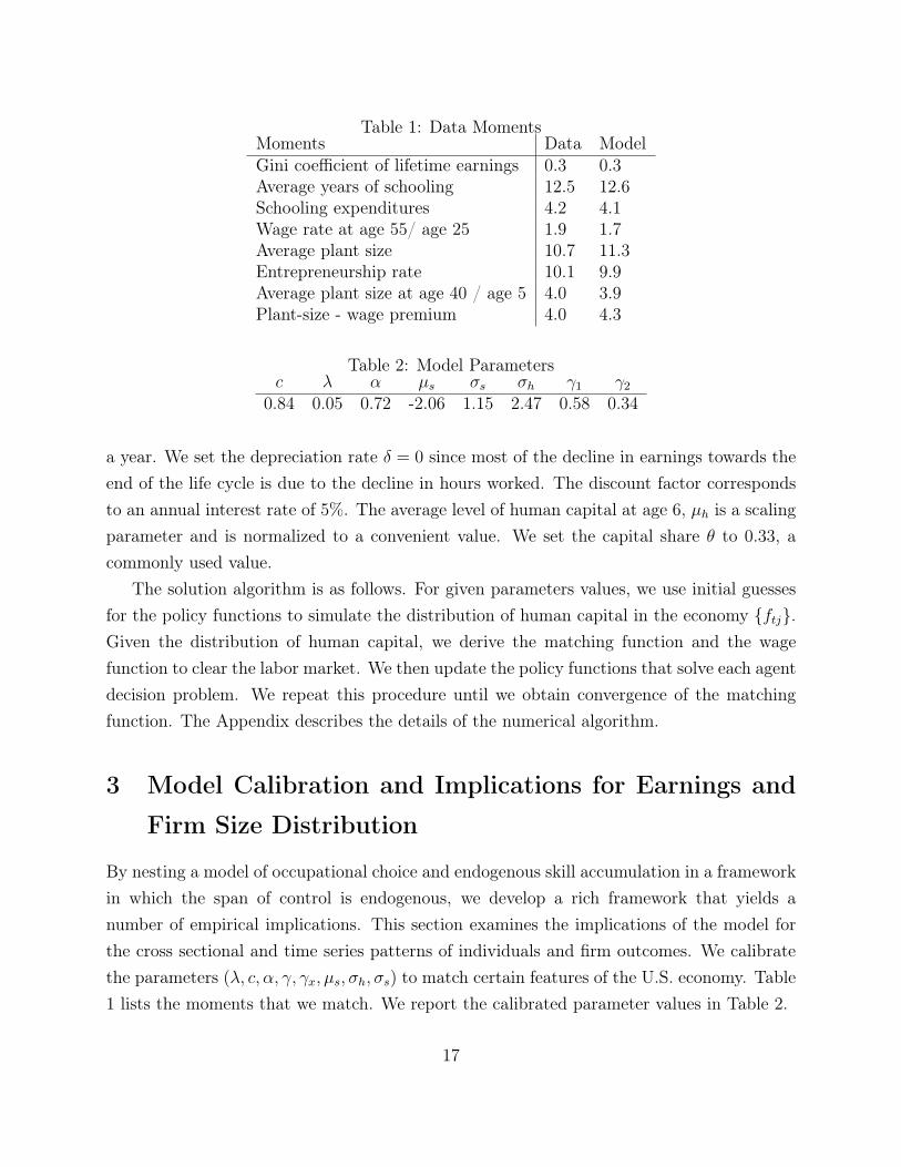
Table 1: Data MomentsMoments Data ModelGini coefficient of lifetime earnings 0.3 0.3Average years of schooling 12.5 12.6Schooling expenditures 4.2 4.1Wage rate at age 55/ age 25 1.9 1.7Average plant size 10.7 11.3Entrepreneurship rate 10.1 9.9Average plant size at age 40 / age 5 4.0 3.9Plant-size - wage premium 4.0 4.3
Table 2: Model Parametersc � ↵ µ
s
�
s
�
h
�1 �2
0.84 0.05 0.72 -2.06 1.15 2.47 0.58 0.34
a year. We set the depreciation rate � = 0 since most of the decline in earnings towards theend of the life cycle is due to the decline in hours worked. The discount factor correspondsto an annual interest rate of 5%. The average level of human capital at age 6, µ
h
is a scalingparameter and is normalized to a convenient value. We set the capital share ✓ to 0.33, acommonly used value.
The solution algorithm is as follows. For given parameters values, we use initial guessesfor the policy functions to simulate the distribution of human capital in the economy {f
tj
}.Given the distribution of human capital, we derive the matching function and the wagefunction to clear the labor market. We then update the policy functions that solve each agentdecision problem. We repeat this procedure until we obtain convergence of the matchingfunction. The Appendix describes the details of the numerical algorithm.
3 Model Calibration and Implications for Earnings and
Firm Size Distribution
By nesting a model of occupational choice and endogenous skill accumulation in a frameworkin which the span of control is endogenous, we develop a rich framework that yields anumber of empirical implications. This section examines the implications of the model forthe cross sectional and time series patterns of individuals and firm outcomes. We calibratethe parameters (�, c,↵, �, �
x
, µ
s
, �
h
, �
s
) to match certain features of the U.S. economy. Table1 lists the moments that we match. We report the calibrated parameter values in Table 2.
17

Some of the moments we target are fairly standard. We target 12.5 years of schoolingfollowing Barro and Lee (2013). The Gini coefficient of lifetime earnings is set to 0.3 whichis the typical value that has been calculated using the PSID. This provides information onindividuals heterogeneity in our model, and in particular the parameter �
s
and �
h
. Accordingto the UNESCO Institute for Statistics, schooling expenditures represents 4.2% of GDP. Itis useful to pin down the share of intermediate inputs in the human capital productiontechnology �2.
The remainder of this Section discusses how other moments help pin-down the modelparameters. Our model is parsimoniously calibrated and for this reason we chose a con-servative strategy. Some forces outside the model are likely to affect the moments we usedand we took some care reflecting these concerns in our calibration strategy. As a result, thecalibration leads to a fairly high communication cost c: the main benefit of creating firmsfor talented individuals is to allow them to deal with exceptions and spread their humancapital over a larger scale.
3.1 Firm Heterogeneity
We consider an economy where individuals skills are central determinants of firm size, pro-ductivity and wages. As in Lucas (1978), entrepreneurial talent determines firm productivityin the sense that an entrepreneur endows his workers with his own human capital. A firm’sproductivity is equal to AG(h
e
) where h
e
is the entrepreneur human capital. Hence, atan efficient allocation, there exists dispersion in productivity across firms because some en-trepreneurs are more talented than others. The existence of productivity dispersion acrossfirms in equilibrium is a feature of several economic models. What is new to our framework isthat labor productivity is not equalized across firms even though the allocation of human cap-ital is efficient. We consider a production technology where the efficiency units assumptiondoes not hold: labor quantity is an imperfect substitute for labor quality. Hence, the averageproductivity of labor is not equalized across firms. High productivity firms attract high pro-ductivity employees which keeps labor productivity high. Further because of the constrainton entrepreneur time, high productivity firms are large since the best entrepreneurs attractthe best workers which allow them to delegate a larger set of tasks and only use their limitedtime for the more difficult problems. On the other hand, low quality entrepreneurs attractlow quality workers leading to a low productivity of labor. Labor productivity dispersion isnot due to idiosyncratic distortions and is instead due to the sorting between heterogeneousentrepreneurs and heterogenous workers.
18
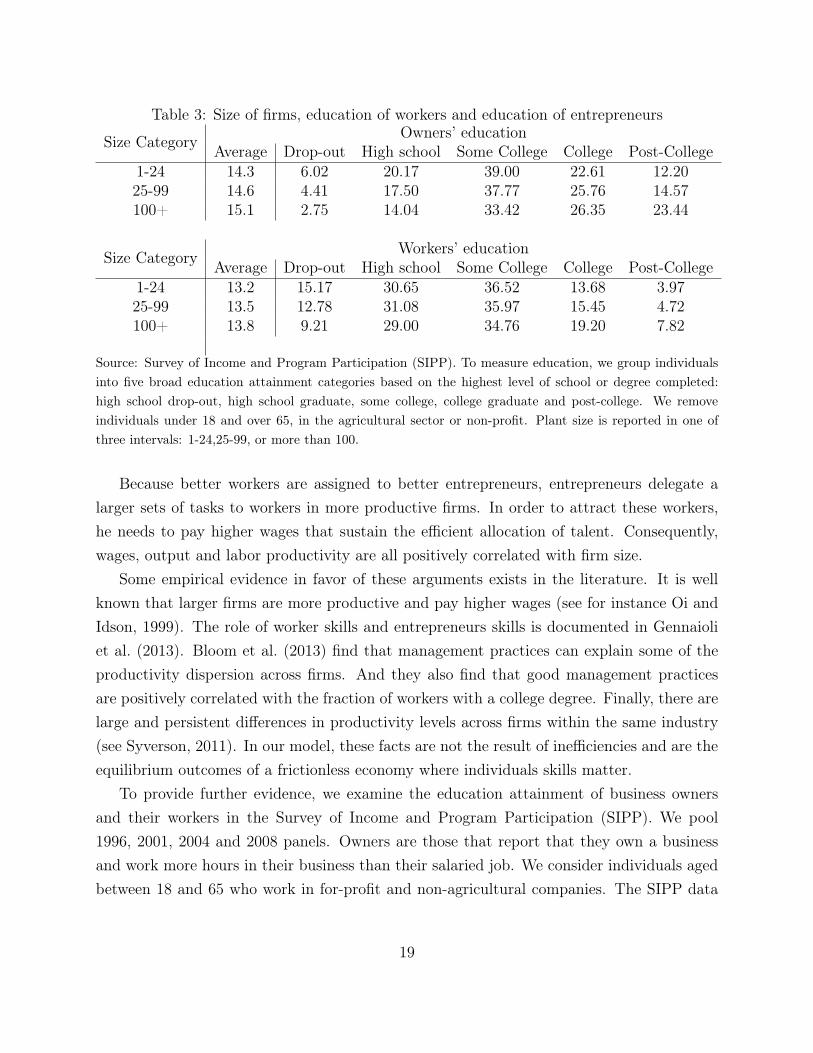
Table 3: Size of firms, education of workers and education of entrepreneurs
Size Category Owners’ educationAverage Drop-out High school Some College College Post-College
1-24 14.3 6.02 20.17 39.00 22.61 12.2025-99 14.6 4.41 17.50 37.77 25.76 14.57100+ 15.1 2.75 14.04 33.42 26.35 23.44
Size Category Workers’ educationAverage Drop-out High school Some College College Post-College
1-24 13.2 15.17 30.65 36.52 13.68 3.9725-99 13.5 12.78 31.08 35.97 15.45 4.72100+ 13.8 9.21 29.00 34.76 19.20 7.82
Source: Survey of Income and Program Participation (SIPP). To measure education, we group individualsinto five broad education attainment categories based on the highest level of school or degree completed:high school drop-out, high school graduate, some college, college graduate and post-college. We removeindividuals under 18 and over 65, in the agricultural sector or non-profit. Plant size is reported in one ofthree intervals: 1-24,25-99, or more than 100.
Because better workers are assigned to better entrepreneurs, entrepreneurs delegate alarger sets of tasks to workers in more productive firms. In order to attract these workers,he needs to pay higher wages that sustain the efficient allocation of talent. Consequently,wages, output and labor productivity are all positively correlated with firm size.
Some empirical evidence in favor of these arguments exists in the literature. It is wellknown that larger firms are more productive and pay higher wages (see for instance Oi andIdson, 1999). The role of worker skills and entrepreneurs skills is documented in Gennaioliet al. (2013). Bloom et al. (2013) find that management practices can explain some of theproductivity dispersion across firms. And they also find that good management practicesare positively correlated with the fraction of workers with a college degree. Finally, there arelarge and persistent differences in productivity levels across firms within the same industry(see Syverson, 2011). In our model, these facts are not the result of inefficiencies and are theequilibrium outcomes of a frictionless economy where individuals skills matter.
To provide further evidence, we examine the education attainment of business ownersand their workers in the Survey of Income and Program Participation (SIPP). We pool1996, 2001, 2004 and 2008 panels. Owners are those that report that they own a businessand work more hours in their business than their salaried job. We consider individuals agedbetween 18 and 65 who work in for-profit and non-agricultural companies. The SIPP data
19
report plant size in one of three intervals: 1-24, 25-99, or more than 100. For each plantsize category, Table 3 reports average years of education and the proportion of businesseswhose owners’ education falls into five broad education attainment categories measured bythe highest level of school or degree completed: high school drop-out, high school graduate,some college, college graduate and post-college. Similarly, for each size category we report theproportion of workers in each schooling category. Larger firms are owned by more educatedindividuals. More than 50% of firms with more than 100 employees are owned by workerswith at least a college degree as opposed to 35% for firms with less than 25 employees.Similarly, larger firms employ more educated workers. For instance, firms with more than100 employees have more than twice as many employees with a post-college degree relativeto firms with less than 25 employees.
We also look at the impact of plant size on worker wage. This helps separate workerssolving problems from workers supplying raw labor in our model. Because the efficiency unitsassumption holds only for the latter, a strong plant size-wage correlation is informative onthe fraction of workers for which sorting matters. The wage measure is a self-reported hourlywage. Table 4 lists the coefficient on each plant size category dummy from the regressionof log wage on plant size controlling for race, gender, age, industry and occupation. Theresults are presented with and without education dummies in, respectively, Column (1) andColumn (2). Workers receive 17% more pay in establishments of 100+ workers than in plantswith 1-24 workers and the corresponding coefficient is statistically significant. The plant-size wage gap percentage between plants with 25-99 workers and firms with 1-24 workers isalso statistically significant and below 3%. The specification with education dummies onlyslightly attenuates the coefficient on plant size. This is as expected from our theory sinceeducation is an imperfect proxy for skills. It also suggests there are other motives that leadslarger firms to pay higher wages. In our calibration, we target a premium of 4% which is inthe lower range of the estimates reported in the literature (see the survey by Oi and Idson,1999).
3.2 The Life-Cycle of Wages and Firms
The life-cycle of earnings and firm size have been documented in several papers but rarelyhave the two facts been connected. For instance, earnings of high school graduates increaseby about 50% in the first 10 years of their working life in the PSID. On the firm side, it is wellknown that conditional on survival, young firms grow more rapidly than their more maturecounterparts. Our model captures both facts simultaneously. Wages grow over time through
20
Table 4: Wage - Firm Size PremiumVariables (1) (2)
25-99 0.0272 0.0251(75.87) (72.93)
100+ 0.1741 0.1615(101.11) (91.91)
Education Dummies No YesObservations 318680 318680
R
2 0.2272 0.3254Source: Survey of Income and Program Participation (SIPP). Wage measure is self-reported hourly wagerate. OLS regression of log wage on dummies for each plant size bin controlling for age, race, gender, industryand occupations. The Table reports the number of observations and the R2. t-stats are shown in parentheses.
three channels: (1) human capital accumulation h
w
, (2) time spent in production n
w
and (3)matching with a better entrepreneur m0
(h
w
) > 0. The first two channels are standard in anyhuman capital accumulation model dating back to at least Ben-Porath (1967). Most modelsof human capital accumulation do not attribute a role to the firm in explaining earningsgrowth of workers. Yet, matched employer-employee datasets (see Abowd et al. (1999) andmore recently Card et al. (2013)) reveal the importance of firms in explaining individualearnings. This is exactly what our theory predicts: some of the earnings of an individual aredue not only to his own human capital but also to the human capital of his entrepreneur.Similarly, the size of a firm grows through three channels: (1) the accumulation of humancapital h
e
, (2) time spent in production n
e
and (3) the ability to attract better workersm
�10(h
e
) > 0.We use these two features to discipline our model parameters. For individuals, the target
value for the earnings growth is the ratio of wage rate at age 55 and wage rate at age 25 whichis 1.9 in the PSID. This number is similar to the figure reported in studies that estimatelifecycle earnings profiles from the PSID. For firms, we use the numbers reported in Hsiehand Klenow (2014). They find that in the cross-section, the average plant over the age offorty is about eight times larger than the average plant under the age of 5. Following a cohortof new establishments in 1967, they find an even larger number: average plant size increasesby a factor of 10 from birth to age 25. However, some growth in average employment of acohort can be attributed to the exit of small establishments. Survivors grow by a factor of4. Since our model is silent on entry and exit, we set the growth of firms to be equal to 4which is a conservative number.
21
3.3 Occupational Choice
According to our model, entrepreneurs are on average older than workers and have a higherlevel of human capital. This is because human capital increases over time and consequentlypeople cross the threshold after a certain age. In the calibrated model, the fraction ofentrepreneurs increases from less than 5% at age 20 to around 15% at age 40. The highlearning-ability types have a higher fraction of entrepreneurs. With 5 learning-ability types,the lowest group has fewer than 5% of entrepreneurs while the highest group has more than20% of entrepreneurs. It formalizes an insight of Lucas (1978):
people tend to move from employee to managerial status later in their careers(as opposed to immediately upon entry to the workforce, as predicted by thetheory above); those that make this transition tend to be among the most skilledemployees. These facts suggest the existence of a kind of human capital which isproductive both in managing and in working for others, and which is accumulatedmost rapidly as an employee.
These empirical implications can be found in the data. First, Table 3 showed that en-trepreneurs are on average more educated than workers. Second, we look at the AmericanCommunity Survey for 2008 to report the fraction of entrepreneurs by age. We use twodifferent measures. The first one is the closest to the model and defines entrepreneurs inthe data as being a business owner as opposed to being employed (and working for someoneelse). The fraction of business-owners in the data is 10.1% which we include as a calibrationtarget. A broader interpretation of our model, sometimes adopted in the literature using hi-erarchical models,10 is to interpret the agents at the top of organization as managers. Usingthe occupation categories defined by Autor and Dorn (2013), we consider both the narrowcategory composed of “Chief executives” and the broader category “Executives, Administra-tive and Managerial Occupations”. In 2008, the proportion of CEOs in the sample is 0.7%while the proportion of individuals in the broad Managerial category is about 10.4%.
Figure 1 reports how the fraction of the population in one these categories varies byage on a log scale. Consistent with our model, the proportion of individuals choosing theseparticular occupation categories goes up with age. While about 0.1% of the population iscategorized as CEO at age 20, this proportion rises to 1% at age 40 and remains constantuntil retirement. Similarly, the fraction of individuals classified as managers is about 2% atage 20, rises quickly to 8% at age 30 and reaches a plateau of 15% at age 40 until retirement.
10See for instance Caliendo et al. (2014).
22
510
1520
10.
50.
1Pe
rcen
tage
(log
sca
le)
20 30 40 50 60 70Age
Business Owner
CEO
Managerial Occupations
Share of Entrepreneurs by Age
Figure 1: Occupational Choice by AgeSource: American Community Survey for 2008. Occupation measure refers to prior year’s employment. Thefigure plots the percentage of the population in one of the three entrepreneurs measures by age for individualsbetween 18 and 65 years old. The y-axis is on log scale.
The fraction of business owners closely track the fraction of managers but show a steady risewith age.
A statistic closely related to occupational choice is the average plant size.11 Hence, wehence include it as a calibration target. Using the U.S. Economics Census, we find thataverage plant size is 10.7 once we take into account self-entrepreneurs (to which we assignzero employees by construction). This helps pin down the communication cost c and theparameter of the problem distribution �. We focus on the average plant size since it has aclear interpretation in our model. Our model could be extended in two directions to fit theentire firm size distribution. First, we could generalize the technology to more than two layersof production. Without additional sources of heterogeneity across firms, the equilibrium canonly sustain two connected levels of hierarchy (see Garicano and Rossi-Hansberg (2006) fora formal proof). In such a setting, it is natural to think about a firm made of a managerand several employees. To have more than two connected levels of hierarchy it is necessaryto introduce an additional source of heterogeneity. Caliendo and Rossi-Hansberg (2012)provide this extension where firms sell products of different qualities. We do not pursue it
11They are approximately the inverse of one another.
23
here since the distribution of product qualities is likely to differ across countries and it wouldnot change the qualitative predictions of the model. Second, we assume that firms have afinite horizon that corresponds to the working horizon of entrepreneurs. An extension of themodel would consider how entrepreneurs could sell or transmit their human capital to otherindividuals when they retire.
With the proposed calibration, it turns out that entrepreneurs spend less time accumu-lating human capital than workers. There are three different forces at play. First, they havea higher opportunity cost of human capital accumulation. Second, to become entrepreneursthey must have previously accumulated a sufficiently high level of human capital. Finally,there is an opposing force: entrepreneurs have on average a higher learning ability and shouldaccumulate more human capital all else equal. With the proposed calibration, the first twoeffects dominate.
4 Implications of the Model for Cross-Countries Differ-
ences
This section examines the implications of the model for cross-countries differences in theorganization of production. To discipline our quantitative exercise, we match output percapita differences by varying the aggregate efficiency level z controlling for exogenous differ-ences in demographic variables and the price of physical capital. This parameter z capturesthe various aggregate factors, such as institutions, geography, culture or luck, that impactoutput conditional on inputs.
We then examine our model ability to match firm size, firm growth, occupational choice,and firm-level productivity dispersion across countries. We find that individuals skills andhuman capital accumulation can substantially improve our understanding of these cross-countries regularities.
4.1 Cross-Countries Differences in Income
The first step to our cross-countries analysis is to vary the aggregate efficiency level z tomatch output per capita differences. We use the implied variations to evaluate the abilityof our model to quantitatively explain differences in the organization of production acrosscountries due to individuals skills and human capital accumulation decisions.
Table 5 reports GDP by deciles of output per worker from Penn World Table 8.0. There
24

Table 5: Cross-Countries Differences in GDP and aggregate efficiency.Decile GDP per capita Lifespan Fertility p
k
z
US 1 77 2.07 1.00 190-100 0.87 80 1.65 1.00 0.9380-90 0.74 79 1.87 0.97 0.8170-80 0.51 76 1.45 1.14 0.6860-70 0.35 74 1.91 1.23 0.6050-60 0.25 70 1.87 1.35 0.5240-50 0.19 71 2.41 1.10 0.4230-40 0.12 66 2.69 1.47 0.3720-30 0.08 62 3.58 1.44 0.2820-10 0.04 54 4.44 1.34 0.220-10 0.02 53 4.79 1.22 0.15
Source: Penn World Table 8.0 (PWT 8.0), World Bank and CIA World Fact-book. GDP per capita ismeasured as average Real GDP over the years 2003 and 2007 at constant 2005 national prices divided bytotal workforce. Life expectancy comes from life expectancy at birth from the World Bank. The Fertilityrate is measured at the total fertility rate adjusted for the infant mortality rate taken from the CIA WorldFactbook. The relative price of capital pk is measured as the ratio of the “price level of capital formation”relative to the “price level of household consumption” from the PWT 8.0 and averaged over the years 2003-2007.
are large variations across countries in standards of living. We choose the value of z in eachdeciles to match output per worker allowing for exogenous differences in lifespan and fertilityrate (which determines the age structure of population) and the price of capital. The lastcolumn of Table 5 reports the implied differences in aggregate efficiency normalizing z toone in the US.
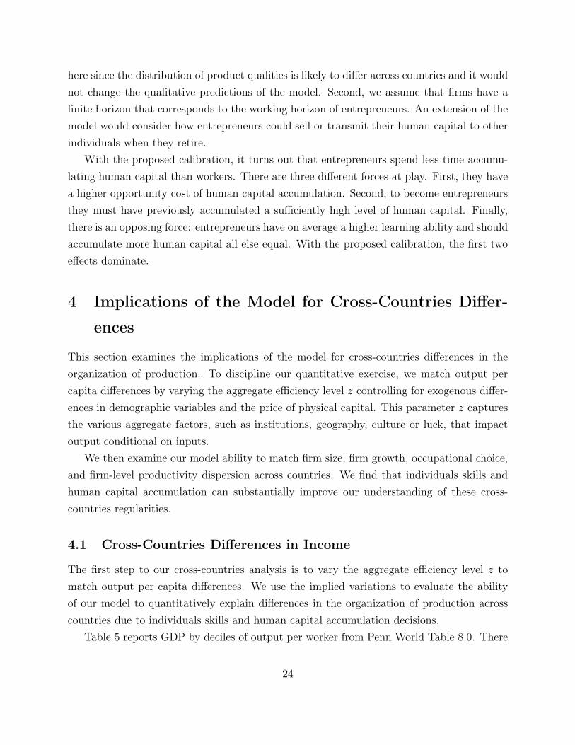
Under our calibration strategy, human capital strongly amplifies aggregate efficiencydifferences across countries: a 7-fold difference in z explains a 50-fold difference in outputper worker as is observed between the top 10 percent and bottom 10 percent of countries. Theamplification lies in between the numbers reported by Erosa et al. (2010) and Manuelli andSeshadri (2014). We borrow from these two papers the idea that producing human capitalrequires some physical inputs which are more efficiently produced in richer countries.12 Wenow turn our attention to how the human capital of workers and entrepreneurs vary acrosscountries. Figure 2 reports the evolution of the problem solving-ability of different groupsof individuals in the economy for different level of aggregate efficiency z.
Workers and entrepreneurs both have higher levels of human capital in richer countries.12We have performed the exercise of this Section using a lower share of intermediate inputs in the produc-
tion of human capital. As expected, it leads to a larger role for differences in z across countries but leavesthe qualitative implications for the organization of production unaffected.
25
0.1
.2.3
Frac
tion
of p
robl
ems
solv
ed
.2 .4 .6 .8 1Aggregate efficiency
Workers
Entrepreneurs
Population
Marginal Individual
Human capital of workers, entrepreneurs and economic development
Figure 2: Human Capital of Workers, Entrepreneurs and Economic Development
The average problem-solving ability of entrepreneurs (workers) differs by a factor of 1.5 (6)between the top and the bottom deciles. These cross country variations in the distribution ofhuman capital arise because of individual incentives to accumulate human capital that differdepending on the aggregate level of efficiency of the economy. Further, the average humancapital of entrepreneurs is higher than the average human capital of workers in every countryreflecting the fact that it is optimal for the most skilled individuals to become entrepreneursand organize production carried out by less talented individuals.
The problem-solving ability of the marginal individual helps illustrate the main mecha-nism driving the negative relationship between the share of entrepreneurs and output percapita described in the next subsection. In the poorest country, the marginal entrepreneurhas about the same talent as the average individual in the population. As aggregate effi-ciency increases, the threshold to become entrepreneur h⇤ increases, reflecting the fact that itrequires more and more talent to become an entrepreneur as the economy gets richer. Andthe average talent of workers increases in the population permitting the creation of largefirms. As the result, it requires a disproportionate amount of talent to be an entrepreneur ina richer economy where the gap between the marginal individual and the average individualis larger than in poorer countries.
Are the predictions of the model in line with estimates of human capital? While humancapital is not directly observable, these decisions can be traced back to schooling and onthe job-training statistics. In the dataset constructed by Barro and Lee (2013), averageyears of schooling are 12.5 in the US, 8.5 in the median country and 3.6 in the lowest decile
26
of income. Our model predicts, respectively, 12.6, 9.3 and 2.8. As for on-the-job trainingdecisions, one measure is the steepness of earnings-profile. Lagakos et al. (2012) documentthat experience-earnings profiles are flatter in poor countries suggesting that lifecycle humancapital accumulation is less intense in poorer countries. This is precisely what our modelpredicts.
Having disciplined our estimates of the aggregate efficiency z of different countries, we cannow examine the impact on the organization of production. We first look at the implicationsfor average plant size and occupational choice. Then, we look at firm growth and finally thedispersion of labor productivity.
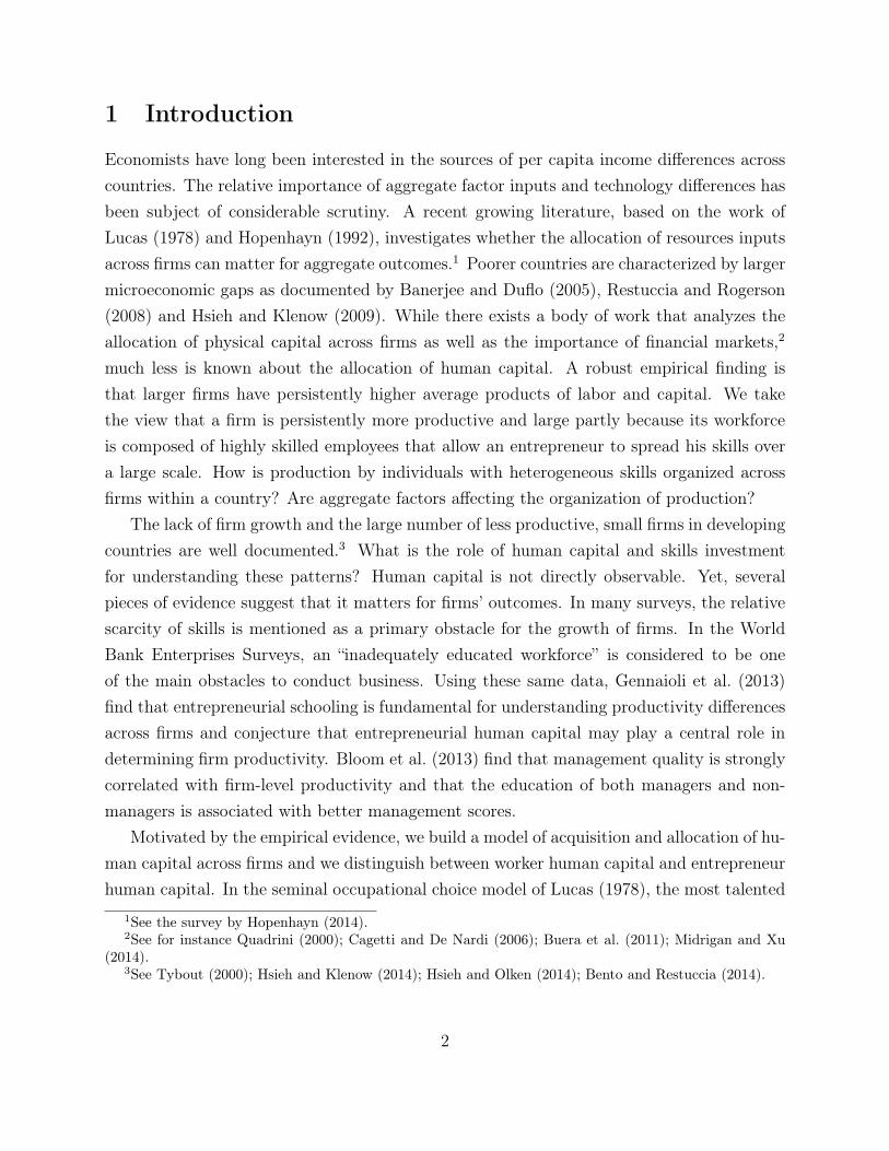
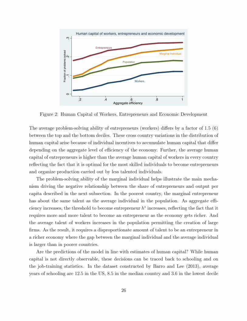
4.2 Plant Size and Occupational Choice
Comparable firm size distributions across countries are notoriously difficult to find. Yet,some broad patterns have been reported in several studies.13 Two robust facts are thepositive relationship between average plant size and GDP per capita as well as the negativerelationship between the entrepreneurial rate and GDP per capita. The prevalence of smallerfirms in poor countries has been measured using different metrics and we focus here on theaverage size of a plant since there is a clear mapping between worker quality and plant size inour model. Indeed, average plant size is lower in countries where the average level of humancapital is low. To get a sense for whether the magnitude matches up with the evidence weuse two different data-sets. First, we use the data-set constructed by Bento and Restuccia(2014) which uses census, survey and registry data from more than a hundred countries.We omit countries with a population less than half of one million and countries richer thanthe US. Second, we use the Global Entrepreneurship Monitor (GEM), collected by a not-for-profit company, Global Entrepreneurship Research Association. It conducted individuallevel interviews with representative sample of adult across a wide range of countries. Becauseit is at the individual-level, it captures all the firms, even the very small ones, both in theformal and the informal sectors. We refer the reader to Poschke (2014) which containsadditional details on the sources and the construction of the survey. Each dataset has itsown advantages. The former has a larger sample size for each country and the numbers comesfrom more reliable data sources. The latter has the advantage of being at the individual-leveland is likely to cover small and informal firms better which are prevalent in poorer countries.Figure 3 reports average plant-size by GDP per capita in the data and in the model. The
13See Tybout (2000); Gollin (2008); Ramos and Santana (2013); Poschke (2014); Hsieh and Olken (2014);Bento and Restuccia (2014).
27
01
23
4Av
erag
e Pl
ant S
ize
(in L
og)
6 7 8 9 10 11GDP per capita (in Log)
Data-set from Bento and Restuccia (2014)
01
23
4Av
erag
e Pl
ant S
ize
(in L
og)
9 9.5 10 10.5 11GDP per capita (in Log)
The Global Entrepreneurship Monitor Survey
Plant Size and GDP per capita
Figure 3: Average plant size across countriesSource: Left Panel: The Global Entrepreneurship Monitor (GEM) survey. Average plant size is pooledacross the years 1999 to 2005. Solid line is from the model economy. GDP per Capita is from PWT 8.0.Right Panel: Data from Bento and Restuccia (2014) which combine census, survey and registry data for themanufacturing sector. Each dot represents a country in the database.
magnitudes implied by our model seem in line with evidence even though our exercise doesnot directly attempt to match average plant size across countries. Our model does a betterjob at reproducing the household-level data from GEM and it tends to underestimate averageplant size in the data-set constructed by Bento and Restuccia (2014). This was expectedsince our model considers the decision of finite-lived agents and does not consider firms thathave an horizon longer than their creator.
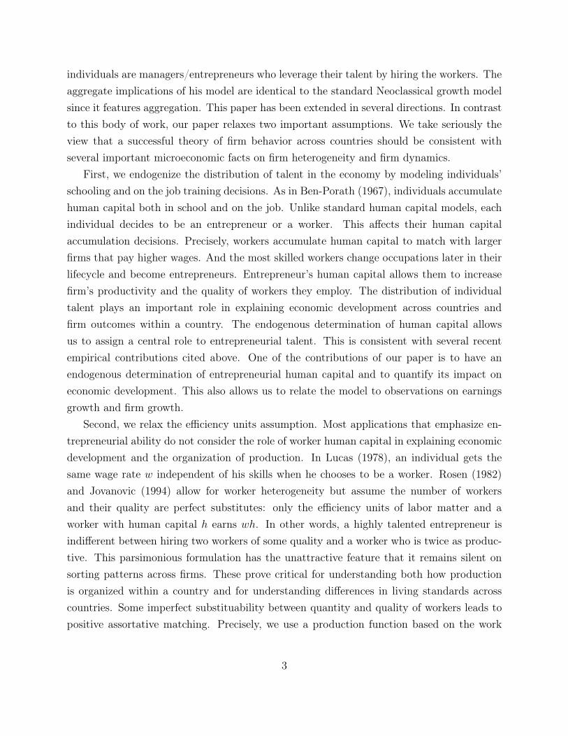
We now examine the implications of our calibrated model for occupational choice acrosscountries. We use two definitions of entrepreneur. First, we use data on the share of en-trepreneurs across different countries from the International Labor Organization (ILO). Wecalculate the proportion of employers and own-account owners in the population. We do notmake a distinction between self-entrepreneurs since what is really critical for us is that asthe economy grows a large fraction of the population decides to work for others and only themost talented individuals hire workers and endow them with their talent. Second, we usedata from IPUMS who report individuals occupations into categories that are harmonizedacross countries. We report the share of individuals in the occupation “Legislators, seniorofficials and managers”. Figure 4 reports the results and performs the same calculations inthe model. The fit is reasonably close to the data in the left panel. The model captures
28
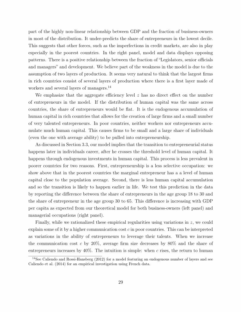
part of the highly non-linear relationship between GDP and the fraction of business-ownersin most of the distribution. It under-predicts the share of entrepreneurs in the lowest decile.This suggests that other forces, such as the imperfections in credit markets, are also in playespecially in the poorest countries. In the right panel, model and data displays opposingpatterns. There is a positive relationship between the fraction of “Legislators, senior officialsand managers” and development. We believe part of the weakness in the model is due to theassumption of two layers of production. It seems very natural to think that the largest firmsin rich countries consist of several layers of production where there is a first layer made ofworkers and several layers of managers.14
We emphasize that the aggregate efficiency level z has no direct effect on the numberof entrepreneurs in the model. If the distribution of human capital was the same acrosscountries, the share of entrepreneurs would be flat. It is the endogenous accumulation ofhuman capital in rich countries that allows for the creation of large firms and a small numberof very talented entrepreneurs. In poor countries, neither workers nor entrepreneurs accu-mulate much human capital. This causes firms to be small and a large share of individuals(even the one with average ability) to be pulled into entrepreneurship.
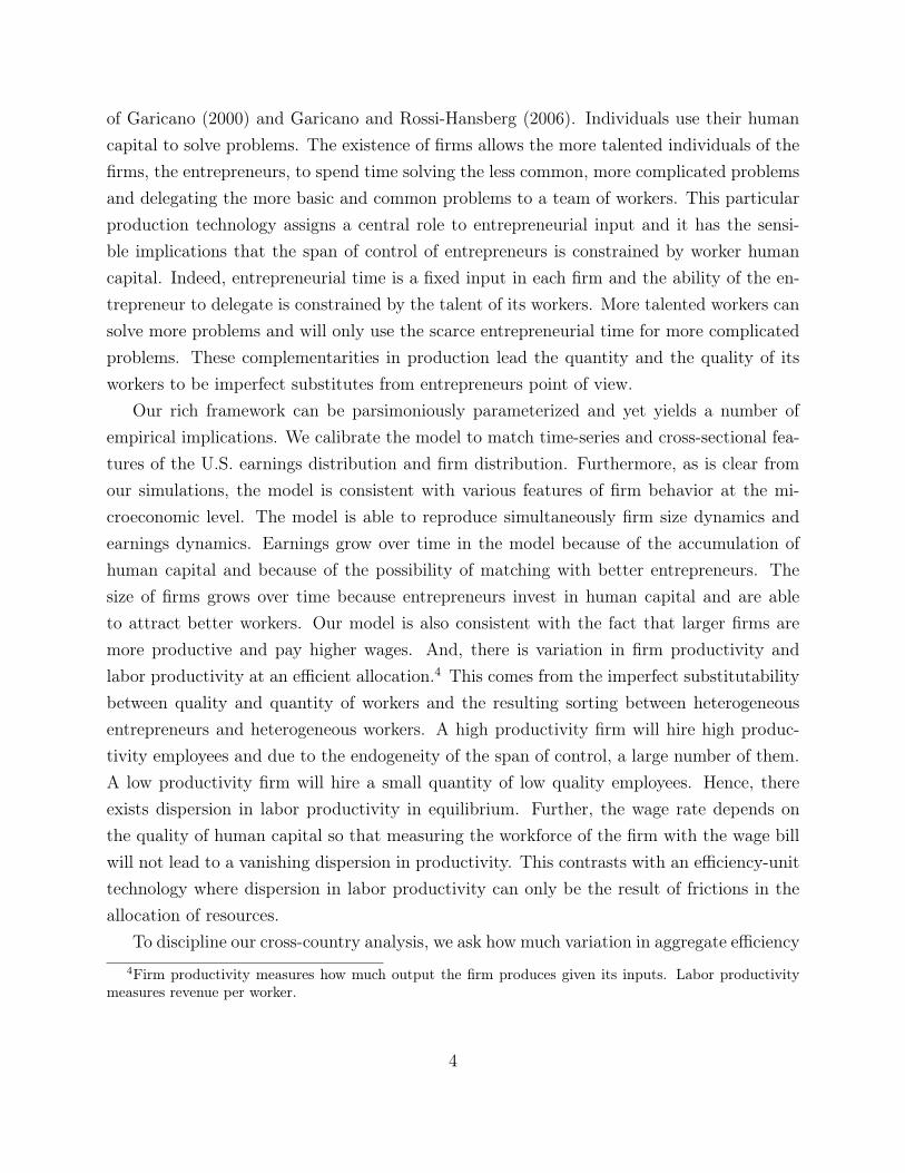
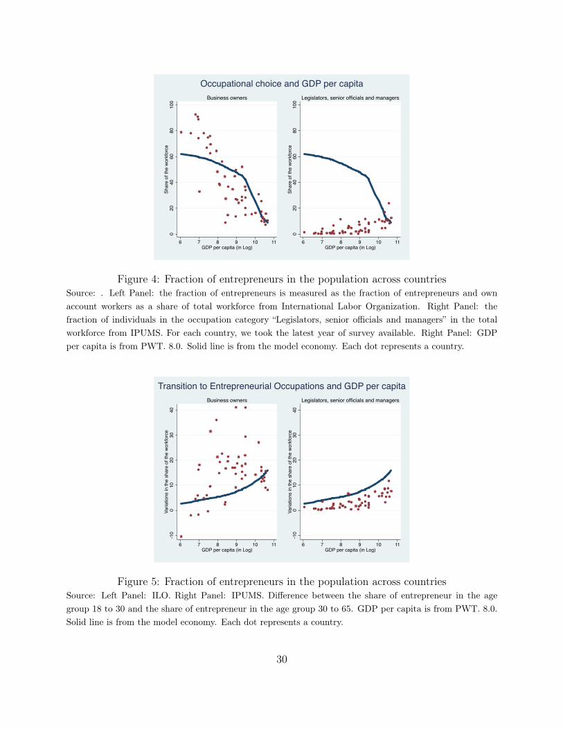
As discussed in Section 3.3, our model implies that the transition to entrepreneurial statushappens later in individuals career, after he crosses the threshold level of human capital. Ithappens through endogenous investments in human capital. This process is less prevalent inpoorer countries for two reasons. First, entrepreneurship is a less selective occupation: weshow above that in the poorest countries the marginal entrepreneur has a a level of humancapital close to the population average. Second, there is less human capital accumulationand so the transition is likely to happen earlier in life. We test this prediction in the databy reporting the difference between the share of entrepreneurs in the age group 18 to 30 andthe share of entrepreneur in the age group 30 to 65. This difference is increasing with GDPper capita as expected from our theoretical model for both business-owners (left panel) andmanagerial occupations (right panel).
Finally, while we rationalized these empirical regularities using variations in z, we couldexplain some of it by a higher communication cost c in poor countries. This can be interpretedas variations in the ability of entrepreneurs to leverage their talents. When we increasethe communication cost c by 20%, average firm size decreases by 80% and the share ofentrepreneurs increases by 40%. The intuition is simple: when c rises, the return to human
14See Caliendo and Rossi-Hansberg (2012) for a model featuring an endogenous number of layers and seeCaliendo et al. (2014) for an empirical investigation using French data.
29
020
4060
8010
0Sh
are
of th
e wo
rkfo
rce
6 7 8 9 10 11GDP per capita (in Log)
Business owners
020
4060
8010
0Sh
are
of th
e wo
rkfo
rce
6 7 8 9 10 11GDP per capita (in Log)
Legislators, senior officials and managers
Occupational choice and GDP per capita
Figure 4: Fraction of entrepreneurs in the population across countriesSource: . Left Panel: the fraction of entrepreneurs is measured as the fraction of entrepreneurs and ownaccount workers as a share of total workforce from International Labor Organization. Right Panel: thefraction of individuals in the occupation category “Legislators, senior officials and managers” in the totalworkforce from IPUMS. For each country, we took the latest year of survey available. Right Panel: GDPper capita is from PWT. 8.0. Solid line is from the model economy. Each dot represents a country.
-10
010
2030
40Va
riatio
ns in
the
shar
e of
the
work
forc
e
6 7 8 9 10 11GDP per capita (in Log)
Business owners
-10
010
2030
40Va
riatio
ns in
the
shar
e of
the
work
forc
e
6 7 8 9 10 11GDP per capita (in Log)
Legislators, senior officials and managers
Transition to Entrepreneurial Occupations and GDP per capita
Figure 5: Fraction of entrepreneurs in the population across countriesSource: Left Panel: ILO. Right Panel: IPUMS. Difference between the share of entrepreneur in the agegroup 18 to 30 and the share of entrepreneur in the age group 30 to 65. GDP per capita is from PWT. 8.0.Solid line is from the model economy. Each dot represents a country.
30
capital accumulation is reduced. Entrepreneurs invest less in human capital and consequentlyfirms do not grow as much. Hence, average firm size declines and there is larger fraction ofentrepreneurs in the population.
4.3 Firm Growth
Hsieh and Klenow (2014) document that the average 40 year old plant employs almost eighttimes as many workers as the typical plant five years or younger in the U.S. In contrast, inpoor countries, plants exhibit little growth in terms of either employment or output. In ourmodel, there are two main channels that may prevent firms from growing in poorer countriesbecause of the low level of human capital in the population. First, the human capitalproduction technology uses both time and intermediate inputs. Intermediate inputs are lessefficiently produced in countries with low aggregate efficiency level z. An entrepreneur hasthen less incentives to spend time away from production to improve his skills. It leads tolower firm growth through the same mechanism that leads workers to invest less in humancapital, resulting in flatter age-earnings profiles. Second, an entrepreneur rewards to skillsimprovement are governed by the possibility to attract better workers and to increase firmsize. The scarcity of talent in poorer countries limits an entrepreneur ability to increase hisspan of control.
There is various survey evidence where business-owners reports the lack of skills to bemajor impediment to the growth of firms in poor countries (see for instance Levy (1993)).We quantitatively examine this possibility in our model. We use data on output per capita,demographics and the price of capital in the US, Mexico and India and examine how farcan our model go towards explaining differences in the life-cycle of plants across countriesas documented by Hsieh and Klenow (2014). Figure 6 reports the model’s predictions.Matching output per capita in Mexico and India requires a z, respectively, 51% and 17%lower than the US level. According to Hsieh and Klenow (2014), controlling for selection,firms grow by a factor of 4 in the US, 2 in Mexico and a little over 1 in India. Our theorypredicts a factor of, 4 in the US, 2.6 in Mexico and 1.4 in India even though the life cycle ofplants in Mexico and India is not used to discipline the model’s parameters.
While the magnitudes are in line with the evidence, our model predict a flattening offirm growth as the entrepreneurs get older. This suggests that other forces are likely toprevent firm growth as a firm age. To match exactly the growth of firms across countries, weexperiment by varying simultaneously z and the communication cost c. The latter parametercan be thought of capturing the level of trust or the probability of theft from employees.
31
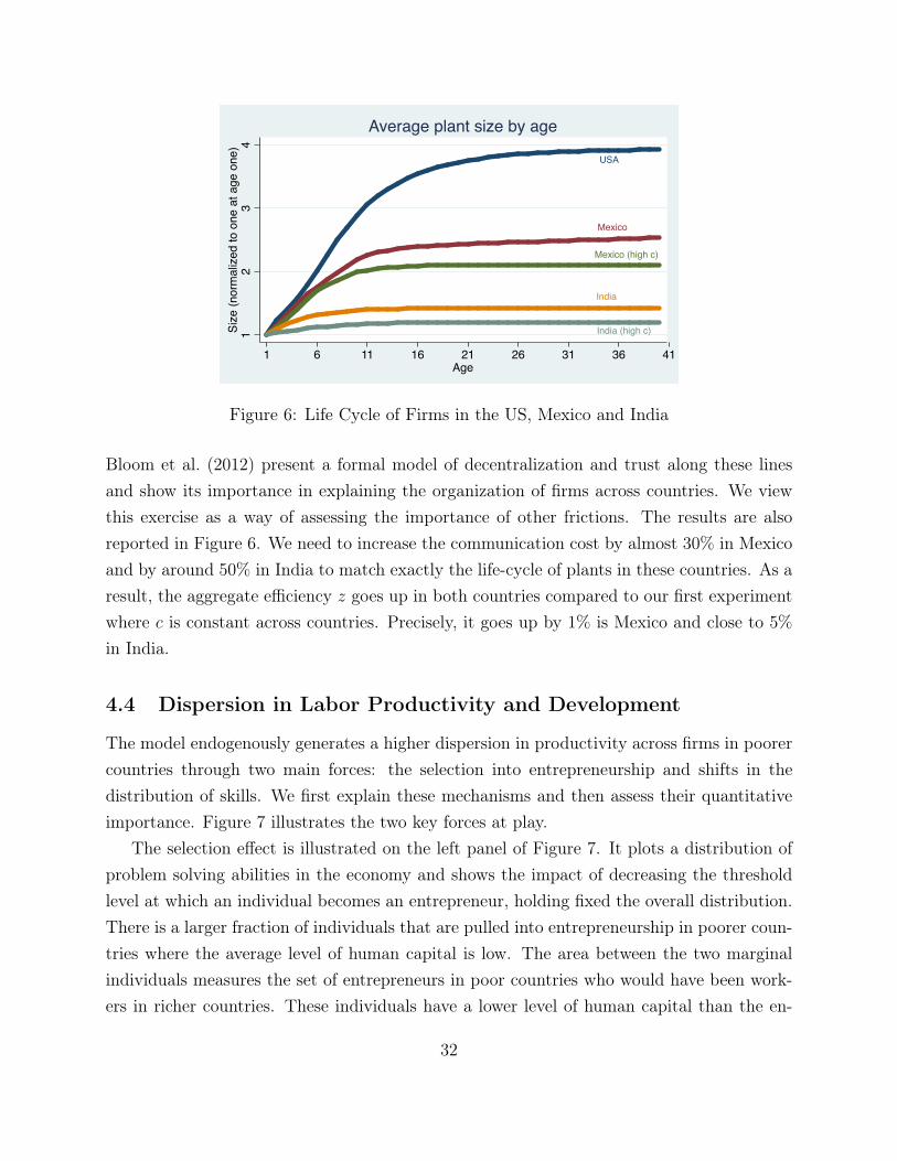
12
34
Size
(nor
mal
ized
to o
ne a
t age
one
)
6 11 16 21 26 31 36 411Age
USA
Mexico
Mexico (high c)
India
India (high c)
Average plant size by age
Figure 6: Life Cycle of Firms in the US, Mexico and India
Bloom et al. (2012) present a formal model of decentralization and trust along these linesand show its importance in explaining the organization of firms across countries. We viewthis exercise as a way of assessing the importance of other frictions. The results are alsoreported in Figure 6. We need to increase the communication cost by almost 30% in Mexicoand by around 50% in India to match exactly the life-cycle of plants in these countries. As aresult, the aggregate efficiency z goes up in both countries compared to our first experimentwhere c is constant across countries. Precisely, it goes up by 1% is Mexico and close to 5%
in India.
4.4 Dispersion in Labor Productivity and Development
The model endogenously generates a higher dispersion in productivity across firms in poorercountries through two main forces: the selection into entrepreneurship and shifts in thedistribution of skills. We first explain these mechanisms and then assess their quantitativeimportance. Figure 7 illustrates the two key forces at play.
The selection effect is illustrated on the left panel of Figure 7. It plots a distribution ofproblem solving abilities in the economy and shows the impact of decreasing the thresholdlevel at which an individual becomes an entrepreneur, holding fixed the overall distribution.There is a larger fraction of individuals that are pulled into entrepreneurship in poorer coun-tries where the average level of human capital is low. The area between the two marginalindividuals measures the set of entrepreneurs in poor countries who would have been work-ers in richer countries. These individuals have a lower level of human capital than the en-
32
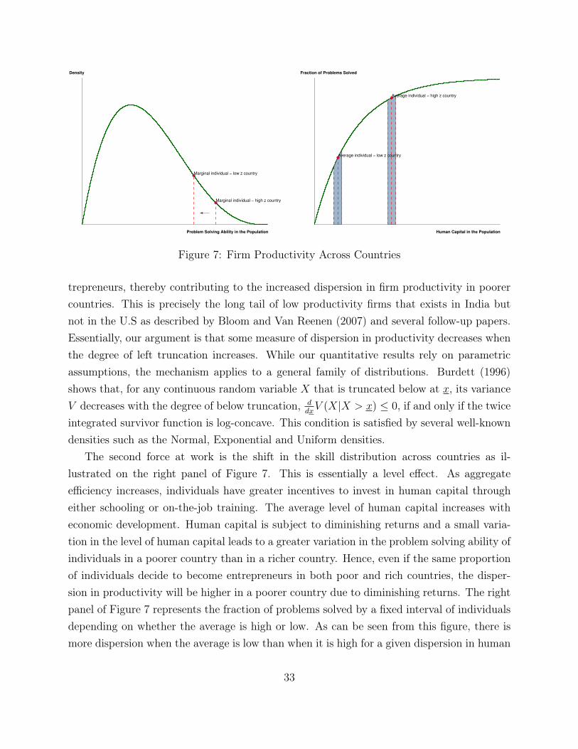
Marginal individual − low z country
Marginal individual − high z country
Problem Solving Ability in the Population
Density
Average individual − high z country
Average individual − low z country
Human Capital in the Population
Fraction of Problems Solved
Figure 7: Firm Productivity Across Countries
trepreneurs, thereby contributing to the increased dispersion in firm productivity in poorercountries. This is precisely the long tail of low productivity firms that exists in India butnot in the U.S as described by Bloom and Van Reenen (2007) and several follow-up papers.Essentially, our argument is that some measure of dispersion in productivity decreases whenthe degree of left truncation increases. While our quantitative results rely on parametricassumptions, the mechanism applies to a general family of distributions. Burdett (1996)shows that, for any continuous random variable X that is truncated below at x, its varianceV decreases with the degree of below truncation, d
dx
V (X|X > x) 0, if and only if the twiceintegrated survivor function is log-concave. This condition is satisfied by several well-knowndensities such as the Normal, Exponential and Uniform densities.
The second force at work is the shift in the skill distribution across countries as il-lustrated on the right panel of Figure 7. This is essentially a level effect. As aggregateefficiency increases, individuals have greater incentives to invest in human capital througheither schooling or on-the-job training. The average level of human capital increases witheconomic development. Human capital is subject to diminishing returns and a small varia-tion in the level of human capital leads to a greater variation in the problem solving ability ofindividuals in a poorer country than in a richer country. Hence, even if the same proportionof individuals decide to become entrepreneurs in both poor and rich countries, the disper-sion in productivity will be higher in a poorer country due to diminishing returns. The rightpanel of Figure 7 represents the fraction of problems solved by a fixed interval of individualsdepending on whether the average is high or low. As can be seen from this figure, there ismore dispersion when the average is low than when it is high for a given dispersion in human
33
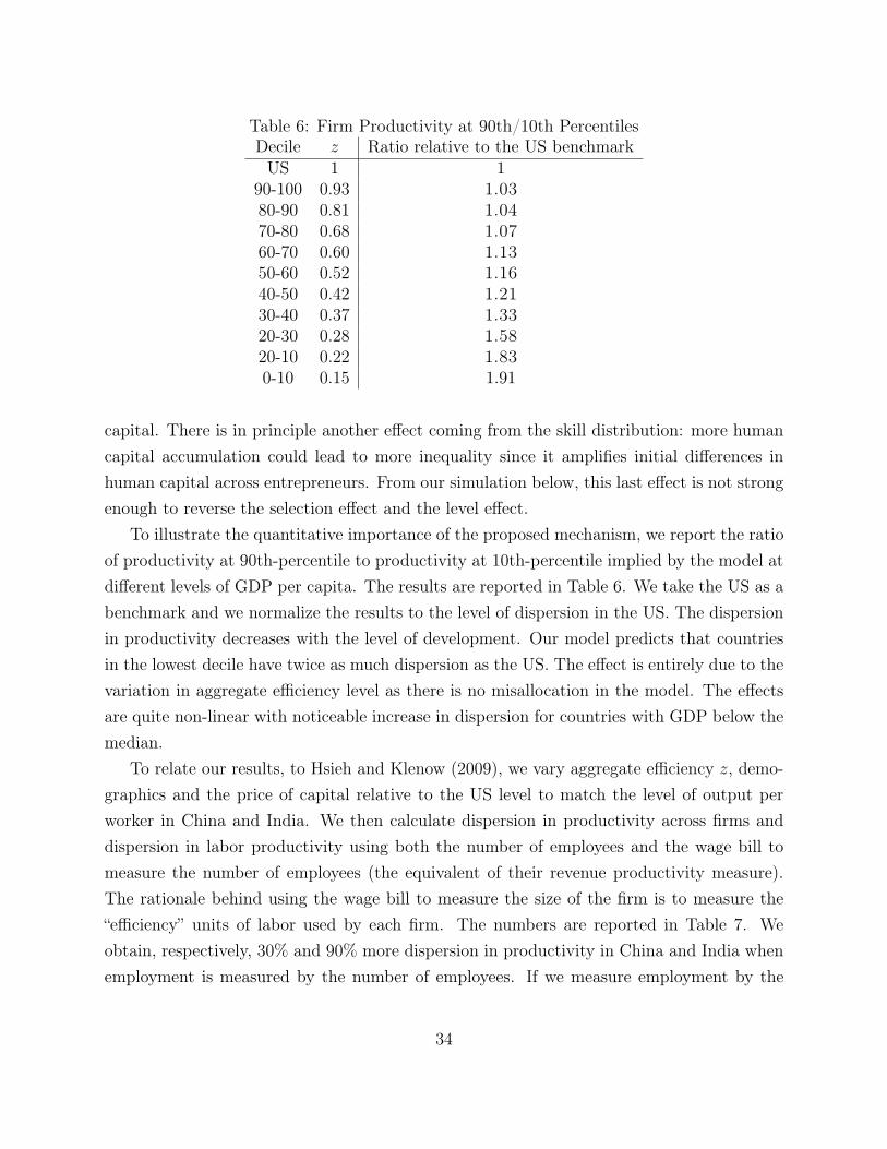
Table 6: Firm Productivity at 90th/10th PercentilesDecile z Ratio relative to the US benchmark
US 1 190-100 0.93 1.0380-90 0.81 1.0470-80 0.68 1.0760-70 0.60 1.1350-60 0.52 1.1640-50 0.42 1.2130-40 0.37 1.3320-30 0.28 1.5820-10 0.22 1.830-10 0.15 1.91
capital. There is in principle another effect coming from the skill distribution: more humancapital accumulation could lead to more inequality since it amplifies initial differences inhuman capital across entrepreneurs. From our simulation below, this last effect is not strongenough to reverse the selection effect and the level effect.
To illustrate the quantitative importance of the proposed mechanism, we report the ratioof productivity at 90th-percentile to productivity at 10th-percentile implied by the model atdifferent levels of GDP per capita. The results are reported in Table 6. We take the US as abenchmark and we normalize the results to the level of dispersion in the US. The dispersionin productivity decreases with the level of development. Our model predicts that countriesin the lowest decile have twice as much dispersion as the US. The effect is entirely due to thevariation in aggregate efficiency level as there is no misallocation in the model. The effectsare quite non-linear with noticeable increase in dispersion for countries with GDP below themedian.
To relate our results, to Hsieh and Klenow (2009), we vary aggregate efficiency z, demo-graphics and the price of capital relative to the US level to match the level of output perworker in China and India. We then calculate dispersion in productivity across firms anddispersion in labor productivity using both the number of employees and the wage bill tomeasure the number of employees (the equivalent of their revenue productivity measure).The rationale behind using the wage bill to measure the size of the firm is to measure the“efficiency” units of labor used by each firm. The numbers are reported in Table 7. Weobtain, respectively, 30% and 90% more dispersion in productivity in China and India whenemployment is measured by the number of employees. If we measure employment by the
34
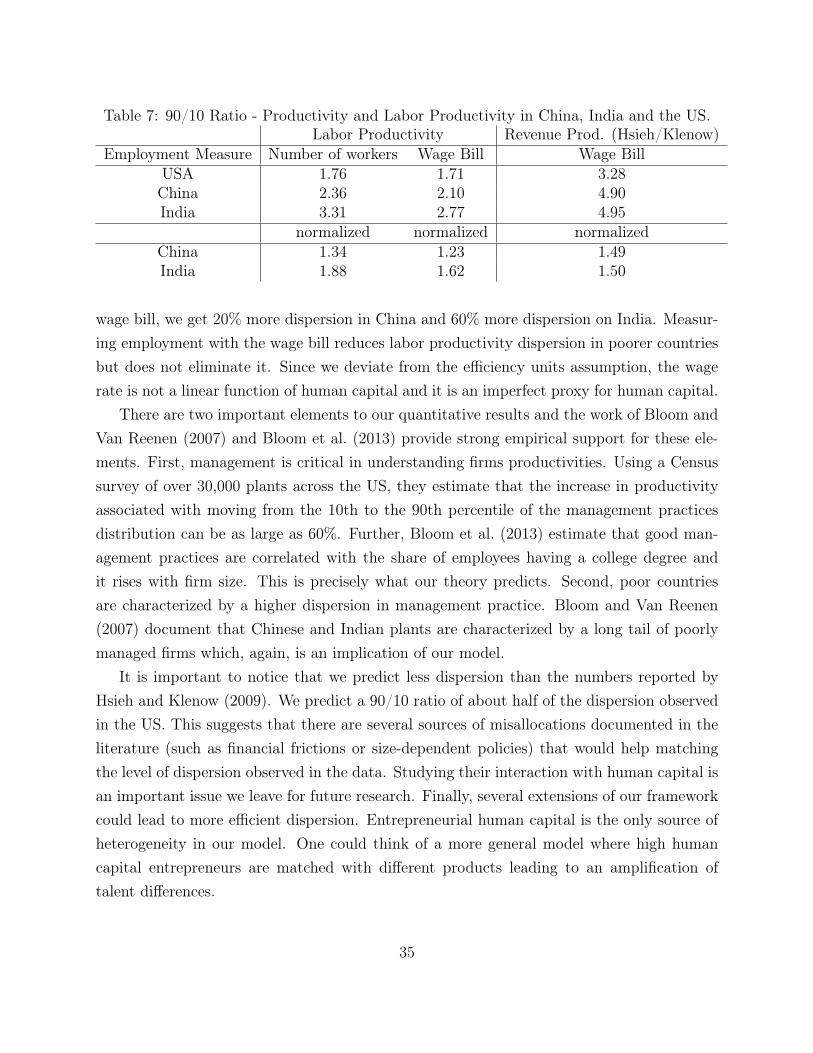
Table 7: 90/10 Ratio - Productivity and Labor Productivity in China, India and the US.Labor Productivity Revenue Prod. (Hsieh/Klenow)
Employment Measure Number of workers Wage Bill Wage BillUSA 1.76 1.71 3.28China 2.36 2.10 4.90India 3.31 2.77 4.95
normalized normalized normalizedChina 1.34 1.23 1.49India 1.88 1.62 1.50
wage bill, we get 20% more dispersion in China and 60% more dispersion on India. Measur-ing employment with the wage bill reduces labor productivity dispersion in poorer countriesbut does not eliminate it. Since we deviate from the efficiency units assumption, the wagerate is not a linear function of human capital and it is an imperfect proxy for human capital.
There are two important elements to our quantitative results and the work of Bloom andVan Reenen (2007) and Bloom et al. (2013) provide strong empirical support for these ele-ments. First, management is critical in understanding firms productivities. Using a Censussurvey of over 30,000 plants across the US, they estimate that the increase in productivityassociated with moving from the 10th to the 90th percentile of the management practicesdistribution can be as large as 60%. Further, Bloom et al. (2013) estimate that good man-agement practices are correlated with the share of employees having a college degree andit rises with firm size. This is precisely what our theory predicts. Second, poor countriesare characterized by a higher dispersion in management practice. Bloom and Van Reenen(2007) document that Chinese and Indian plants are characterized by a long tail of poorlymanaged firms which, again, is an implication of our model.
It is important to notice that we predict less dispersion than the numbers reported byHsieh and Klenow (2009). We predict a 90/10 ratio of about half of the dispersion observedin the US. This suggests that there are several sources of misallocations documented in theliterature (such as financial frictions or size-dependent policies) that would help matchingthe level of dispersion observed in the data. Studying their interaction with human capital isan important issue we leave for future research. Finally, several extensions of our frameworkcould lead to more efficient dispersion. Entrepreneurial human capital is the only source ofheterogeneity in our model. One could think of a more general model where high humancapital entrepreneurs are matched with different products leading to an amplification oftalent differences.
35
5 Conclusion
An active line of work suggests that the allocation of resources within countries is of first-order importance for understanding cross-countries income differences. This paper examineshow productivity differences lead to different forms of organization of production throughits impact on the allocation and accumulation of human capital.
We develop a model of human capital accumulation of workers and entrepreneurs withcomplementarities and sorting combining the work of Ben-Porath (1967), Lucas (1978),Garicano (2000) and Garicano and Rossi-Hansberg (2006). The model yields a numberof empirical implications for earnings and firm heterogeneity within a country. Varyingaggregate efficiency across countries to match GDP per capita differences, we find that humancapital differences can explain a significant part of differences in firm size, firm growth, andoccupational choice. We also show that in our economic environment, where there is only anaggregate variation in efficiency, richer countries are characterized by less firm productivitydispersion and less labor productivity dispersion.
Our model takes seriously the idea that entrepreneur and worker skills are importantfor understanding the organization of firms both within and across countries. We view thispaper as a first step toward understanding the importance of sorting and entrepreneur andworker quality in the allocation of input factors, the organization of firms and economicdevelopment. In particular, these are affected by other factors such as credit markets andtechnology choices. We believe these are of first-order importance and their interaction withhuman capital accumulation decisions is an important topic worthy of further exploration.
To conclude, it is important to underscore that our paper does not suggest the absenceof misallocation, a clear and real feature of the world. Rather we find that the allocation oftalent is likely to differ across of countries with varying levels of efficiency which endogenouslyleads to varying dispersion in firm outcomes. The natural next step is to examine howidiosyncratic distortions lead to different effects in countries with varying level of efficiency.Indeed, the organization of production and endogenous acquisition of skills are likely to leaddistortions to have different impact on countries that are in different stages of development.We leave these questions for future research.
36
References
Abowd, J. M., Kramarz, F., and Margolis, D. N. (1999). High wage workers and high wagefirms. Econometrica, 67(2):251–333.
Antràs, P., Garicano, L., and Rossi-Hansberg, E. (2006). Offshoring in a knowledge economy.The Quarterly Journal of Economics, 121(1):31–77.
Autor, D. and Dorn, D. (2013). The growth of low-skill service jobs and the polarization ofthe U.S. labor market. American Economic Review, 103(5):1553–97.
Banerjee, A. V. and Duflo, E. (2005). Growth theory through the lens of developmenteconomics. Handbook of economic growth, 1:473–552.
Barro, R. J. and Lee, J. W. (2013). A new data set of educational attainment in the world,1950–2010. Journal of Development Economics, 104:184–198.
Becker, G. (1973). A theory of marriage: Part I. The Journal of Political Economy, 81:813–846.
Ben-Porath, Y. (1967). The production of human capital and the life cycle of earnings. TheJournal of Political Economy, 75(4):352–365.
Bento, P. and Restuccia, D. (2014). Misallocation, establishment size, and productivity.Working Paper 517, University of Toronto.
Bhattacharya, D., Guner, N., and Ventura, G. (2012). Distortions, endogenous managerialskills and productivity differences. Review of Economic Dynamics.
Bloom, N., Sadun, R., and Van Reenen, J. (2012). The organization of firms across countries.The Quarterly Journal of Economics, 127(4):1663–1705.
Bloom, N., Sadun, R., and Van Reenen, J. (2013). Management as a technology. mimeo,London School of Economics.
Bloom, N. and Van Reenen, J. (2007). Measuring and explaining management practicesacross firms and countries. The Quarterly Journal of Economics, 122(4):1351–1408.
Buera, F. J., Kaboski, J. P., and Shin, Y. (2011). Finance and development: A tale of twosectors. American Economic Review, 101:1964–2002.
37
Burdett, K. (1996). Truncated means and variances. Economics Letters, 52(3):263–267.
Cagetti, M. and De Nardi, M. (2006). Entrepreneurship, frictions, and wealth. Journal ofPolitical Economy, 114(5):835–870.
Caliendo, L., Monte, F., and Rossi-Hansberg, E. (2014). The anatomy of french productionhierarchies. Journal of Political Economy, forthcoming.
Caliendo, L. and Rossi-Hansberg, E. (2012). The Impact of trade on organization andproductivity. The Quarterly Journal of Economics, 127(3):1393–1467.
Card, D., Heining, J., and Kline, P. (2013). Workplace heterogeneity and the rise of WestGerman wage inequality. The Quarterly Journal of Economics, pages 967–1015.
Chatterjee, S. and Rossi-Hansberg, E. (2012). Spinoffs and the market for ideas. InternationalEconomic Review, 53(1):53–93.
Cooley, T. F. and Quadrini, V. (2001). Financial markets and firm dynamics. AmericanEconomic Review, pages 1286–1310.
Eeckhout, J. and Kircher, P. (2012). Assortative matching with large firms: Span of controlover more versus better workers. Mimeo, University of Edinburgh.
Erosa, A., Koreshkova, T., and Restuccia, D. (2010). How important is human capital?a quantitative theory assessment of world income inequality. The Review of EconomicStudies, 77(4):1421–1449.
Garicano, L. (2000). Hierarchies and the organization of knowledge in production. Journalof Political Economy, 108(5):874–904.
Garicano, L. and Rossi-Hansberg, E. (2006). Organization and inequality in a knowledgeeconomy. The Quarterly Journal of economics, 121(4):1383–1435.
Garicano, L. and Rossi-Hansberg, E. (2012). Organizing growth. Journal of EconomicTheory, 147(2):623–656.
Gennaioli, N., Porta, R., Lopez-de Silanes, F., and Shleifer, A. (2013). Human capital andregional development. The Quarterly Journal of Economics, pages 105–164.
Gollin, D. (2008). Nobody’s business but my own: Self-employment and small enterprise ineconomic development. Journal of Monetary Economics, 55(2):219–233.
38
Grossman, G. M., Helpman, E., and Kircher, P. (2014). Matching, sorting, and the distri-butional impacts of international trade. mimeo, University of Edinburgh.
Hopenhayn, H. A. (1992). Entry, exit, and firm dynamics in long run equilibrium. Econo-metrica, pages 1127–1150.
Hopenhayn, H. A. (2014). Firms, misallocation, and aggregate productivity: A review.Annual Review of Economics, 6(1):735–770.
Hsieh, C.-T. and Klenow, P. (2009). Misallocation and manufacturing TFP in China andIndia. The Quarterly Journal of Economics, 124(4):1403.
Hsieh, C.-T. and Klenow, P. J. (2014). The life cycle of plants in india and mexico. TheQuarterly Journal of Economics, 129(3):1035–1084.
Hsieh, C.-T. and Olken, B. A. (2014). The missing "missing middle". Journal of EconomicPerspectives, 28(3):89–108.
Jovanovic, B. (1982). Selection and the evolution of industry. Econometrica, pages 649–670.
Jovanovic, B. (1994). Firm formation with heterogeneous management and labor skills.Small Business Economics, 6(3):185–191.
Jovanovic, B. (2014). Misallocation and growth. American Economic Review, 104(4):1149–71.
Kennan, J. (2006). A note on discrete approximations of continuous distributions. mimeo,University of Wisconsin Madison.
Kremer, M. (1993). The O-ring theory of economic development. The Quarterly Journal ofEconomics, 108(3):551–575.
Lagakos, D., Moll, B., Porzio, T., and Qian, N. (2012). Experience matters: Human capitaland development accounting. NBER Working Papers 18602, National Bureau of EconomicResearch.
Levy, B. (1993). Obstacles to developing indigenous small and medium enterprises: anempirical assessment. The World Bank Economic Review, 7(1):65–83.
Lucas, R. E. (1978). On the Size Distribution of Business Firms. The Bell Journal ofEconomics, 9(2):508.
39
Manuelli, R. E. and Seshadri, A. (2014). Human capital and the wealth of nations. AmericanEconomic Review, 104(9):2736–62.
McCann, R. J., Shi, X., Siow, A., and Wolthoff, R. P. (2014). Becker meets ricardo: Multi-sector matching with social and cognitive skills. mimeo, University of Toronto.
Midrigan, V. and Xu, D. Y. (2014). Finance and misallocation: Evidence from plant-leveldata. American Economic Review, 104(2):422–58.
Oi, W. Y. and Idson, T. L. (1999). Firm size and wages. Handbook of labor economics,3:2165–2214.
Poschke, M. (2014). The firm size distribution across countries and skill-biased change inentrepreneurial technology. IZA Discussion Paper 7991, IZA.
Quadrini, V. (2000). Entrepreneurship, saving, and social mobility. Review of EconomicDynamics, 3(1):1–40.
Ramos, R. and Santana, G. (2013). Distortions and the size distribution of plants: Evidencefrom cross-country data. mimeo, CEMFI.
Restuccia, D. and Rogerson, R. (2008). Policy distortions and aggregate productivity withheterogeneous establishments. Review of Economic Dynamics, 11(4):707–720.
Rosen, S. (1982). Authority, control, and the distribution of earnings. The Bell Journal ofEconomics, pages 311–323.
Sattinger, M. (1975). Comparative advantage and the distributions of earnings and abilities.Econometrica, pages 455–468.
Syverson, C. (2011). What determines productivity? Journal of Economic Literature,49(2):326–65.
Tybout, J. R. (2000). Manufacturing firms in developing countries: How well do they do,and why? Journal of Economic literature, pages 11–44.
40

Appendix
This Appendix is divided into two parts. We prove Proposition 1 and give the details of thenumerical solution of the model.
5.1 Proof of Proposition 1
Defined the static rental rate as R(h
m
) =
AG(hm)�w(hw)c(1�G(hw)) where h
w
is optimally chosen. Usingthe envelope theorem:
R
0(h
m
) =
Ag(h
m
)
c (1�G(h
w
))
leading the cross-partial derivative to be strictly positive:
dR
0(h
m
)
dh
p
= g(h
w
)
Ag(h
m
)
c (1�G(h
w
))
2 > 0
Since it is a maximum, the objective function is concave. Combined with dR
0(hm)dhp
> 0, onecan apply the implicit function theorem to find that:
@h
m
@h
w
> 0
This proves positive sorting.We now prove that the set of entrepreneurs and the set of workers is connected. By
contradiction. Assume the set of workers W and the set of entrepreneurs E writes as
W = [a1, a2] [ [a3, a4]
E = [a2, a3] [ [a4, a5]
with m(a1) = a2 and m(a2) = a3, Given a1 and a3, we can solve for w13, R13 and a2 on(a1, a3). Given a3 and a5, we can solve for w35, R35 and a4 on (a3, a5). For this to be anequilibrium, we need to make sure that agents in the interval (a3, a5) do not want to formteams with agents in the interval (a1, a3).
Note that R13(a3) = w35(a3). If R13(a3) > w35(a3), agents (workers) with skills a3 + ✏
would like to become entrepreneurs and agents at a2 would be willing to worker for them ata wage marginally larger than w13(a2).If R13(a3) < w35(a3), agents a3�✏ would like to become workers and agent at a4 would like tohire them at a wage marginally higher than R13(a3). We prove that lim
z"a3 R013(z) > w
035(z).
41

There are two cases to consider:(1) w13(a2) < AG (a2). Since R13(a3) = w35(a3),
w
035(a3) = g(a3)
AG(a4)c (1�G(a2))� AG(a3) + w13(a2)
(1�G(a3)) c (1�G(a2))
We want to show
Ag(a3)
c (1�G(a2))> g(a3)
AG(a4)c (1�G(a2))� AG(a3) + w13(a2)
(1�G(a3)) c (1�G(a2))
which simplifies to
G(a4) <1
c
A� w13(a2)
A� AG(a2)
This inequality is necessarily true since G(a4) < 1, c < 1 and w13(a2) < AG (a2).(2) w13(a2) � AG (a2). First we show that
w35(a3) = R13(a3) > AG(a3)
Using the mean value theorem, for some x 2 [a2, a3]
R13(a3)� AG(a3) = (R13(a2)� AG(a2)) +
⇣
R
0
13(x)� Ag(x)
⌘
(a3 � a2)
The first term in the RHS is positive since R13(a2) = w13(a2) and by assumption w13(a2) �AG (a2). Regarding the second term in the RHS it is also positive since
R
013(x) =
Ag(x)
c (1�G(m
�1(x)))
> Ag(x)
and c (1�G(m
�1(x))) < 1. We can then conclude R13(a3) > AG(a3).
Since Ag(a3) < R
035(a3), it is sufficient to show that w
035(a3) < Ag(a3) which simplifies
to
AG(a4)� w35 (a3)
A � AG(a3)< 1
This is true since we proved w35(a3) > AG(a3).We now show that there is a contradiction. Precisely, a4 would like to hire a3 � ✏ at a
42

better wage than what he makes as an entrepreneur. Consider the rents that a4 would getfrom hiring a3 � ✏ at wage R13(a3 � ✏):
⇧(a4, a3 � ✏) =
AG(a4)�R13(a3 � ✏)
c (1�G(a3 � ✏))
lim
✏!0
@⇧(a4, a3 � ✏)
@✏
=
R
013(a3)� w
035(a3)
c (1�G(a3))> 0
Hence there are incentives for agents to form different teams.Finally, we need to prove the existence of a c
⇤> 0 such that the allocation guaranteed to
exist is such that R0(h
⇤) > w
0(z
⇤). Consider the incentives of an entrepreneur with ability h
to hire a worker with ability h
⇤+ ✏. Her profits are given by
⇧(h, h
⇤+ ✏) =
AG(h)�R(h
⇤+ ✏)
c (1�G(h
⇤+ ✏))
lim
✏!0
@⇧(h, h
⇤+ ✏)
@✏
=
w
0(h
⇤)�R
0(h
⇤)
c (1�G(h
⇤))
Substituting w(h
⇤) = R(h
⇤) =
AG(h⇤)�w(h)c(1�G(h)) in the optimal choice of h
w
for h
⇤:
w
0(h
⇤) = g(h
⇤)
c (1�G(h))AG(h)� AG(h
⇤) + w(h)
(1�G(h
⇤)) c (1�G(h))
We want to show that w0(h
⇤) < R
0(h
⇤) which is equivalent to
c <
A� w(h)
(1�G(h))AG(h)
The left-hand side of the inequality provides an upper bound for c.
5.2 Numerical Solution
We use the following algorithm to solve the model.
1. Guess n
mtj
, n
wtj
, j = 1, . . . , J, t = 1, . . . , T to obtain an estimate of ftj
.
2. Guess ˜
h, solve for m and h
⇤ using:
m
0(h) = c (1�G(h))
P
J
i=1
P
T
⌧=1 fti (h)nw⌧ i
(h)
P
J
j=1
P
T
t=1 nmt
(m(h))⇥ f
tj
(m (h))
43

and two boundary conditions:
m(
˜
h) = h
⇤
m (h
⇤) = h
3. solve for w and w(
˜
h) so that
w
0(h
w
) = g(h
w
)
AG(m (h
w
))� w (h
w
)
1�G(h
w
)
and w(h
⇤) satisfies the boundary condition:
AG(h
⇤)� w(
˜
h)
c
⇣
1�G(
˜
h)
⌘
= w(h
⇤)
4. solve for the demand of raw labor l
u
and the supply of raw labor. Adjust ˜
h and goback to Step 2 until reaching the equilibrium in the market for raw-labor.
5. Given m,w,
˜
h, h
⇤, solve the individuals problem by backward induction and discretizingthe state space.
6. Check whether the policy functions and matching function have changed since theprevious iteration. Go back to Step 2 until convergence.
44