Underwater acoustic model-based signal processing applied ... · Calhoun: The NPS Institutional Archive Theses and Dissertations Thesis Collection 1985-09 Underwater acoustic model-based

Calhoun: The NPS Institutional Archive

Theses and Dissertations Thesis Collection

1985-09

Underwater acoustic model-based signal processing

applied to the detection of signals from a planar

array of point source elements

Blount, Richard J. Jr.

Naval Postgraduate School: Monterey, California

http://hdl.handle.net/10945/21597

DUDLEY I IBRARYNAVMONTEREY. CAL

NAVAL POSTGRADUATE SCHOOL

Monterey, California

THESISUNDERWATER ACOUSTIC MODEL-BASED SIGNALPROCESSING APPLIED TO THE DETECTION OFSIGNALS FROM A PLANAR ARRAY OF POINT

SOURCE ELEMENTS

by

Richard J. Blount, Jr.

September 19 85

Thesis Advisor: Lawrence J. Ziomek

Approved for public release; distribution is unlimited

T222798

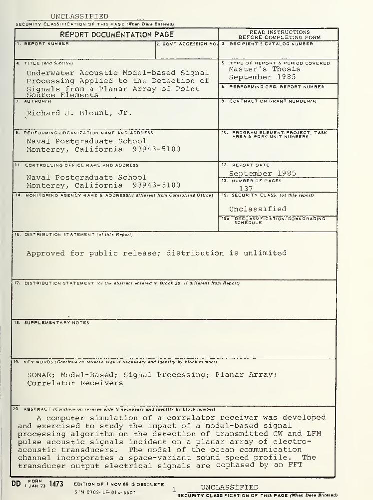
UNCLASSIFIEDSECURITY CLASSIFICATION OF THIS PAGE (Whan Data Entered)

REPORT DOCUMENTATION PAGE READ INSTRUCTIONSBEFORE COMPLETING FORM

1. REPORT NUMBER 2 GOVT ACCESSION NO 3. RECIPIENT'S CAT ALOG NUMBER

4. TITLE (and Subtitle) 5. TYPE OF REPORT & PERIOD COVERED

Underwater Acoustic Model-based SignalProcessing Applied to the Detection ofSignals from a Planar Array of PointSource Elements

Master's ThesisSeptember 1985

6. PERFORMING ORG. REPORT NUMBER

7. AUTHOR*-

*; 8. CONTRACT OR GRANT NUMBERfaj

Richard J. Blount, Jr

9. PERFORMING ORGANIZATION NAME AND ADDRESS

Naval Postgraduate SchoolMonterey, California 93943-5100

10. PROGRAM ELEMENT. PROJECT, TASKAREA ft WORK UNIT NUMBERS

11. CONTROLLING OFFICE NAME AND ADDRESS 12. REPORT DATE


September 198513. NUMBER OF PAGES

13714. MONITORING AGENCY NAME ft ADDRESSfH different from Controlling Office) 15. SECURITY CLASS, (of thlm report)

Unclassified15«. DECLASSIFICATION' DOWNGRADING

SCHEDULE

16. DISTRIBUTION STATEMENT (of this Report)

Approved for public release; distribution is unlimited

17. DISTRIBUTION STATEMENT (ol the abstract entered In Block 20, If different from Report)

18. SUPPLEMENTARY NOTES

19. KEY WORDS (Continue on reverse aide If necessary and Identify by block number)

SONAR; Model-Based; Signal Processing; Planar Array;Correlator Receivers

20. ABSTRACT (Continue on reverse aide If necessary and Identity by block numbsr)

A computer simulation of a correlator receiver was developedand exercised to study the impact of a model-based signalprocessing algorithm on the detection of transmitted CW and LFMpulse acoustic signals incident on a planar array of electro-acoustic transducers. The model of the ocean communicationchannel incorporates a space-variant sound speed profile. Thetransducer output electrical signals are cophased by an FFT

DD, ^N

RM73 1473 EDITION OF 1 NOV 65 IS OBSOLETE

S 'N 0102- LF- 014- 6601UNCLASSIFIED

SECURITY CLASSIFICATION OF THIS PACE (Whan Dmtm Bntmrmd)

UNCLASSIFIEDSECURITY CL ASSlFlC AT ION OF THIS PAGE (Whmt Oat* Bnf*r*<0

#20 - ABSTRACT - CONTINUED

beamformer via phase weighting, and summed to forma total array output signal. The total array outputsignal is correlated with a delayed replica of thetransmit waveform and compared to a Neyman-Pearsonthreshold. Receiver performance is measured using a

Monte Carlo technique to estimate the probability ofdetection for a fixed probability of false alarmversus the signal-to-noise ratio at the input of asingle transducer. White, zero-mean, Gaussian trans-ducer noise is assumed to facilitate comparison betweentheoretical and simulated performance. Results indicatethat model-based signal processing provides significantimprovement of receiver performance.

Approved for public release; distribution is unlimited,

Underwater Acoustic Model-based Signal ProcessingApplied to the Detection of Signals from a

Planar Array of Point Source Elements

by

Richard J. Blount, Jr.Lieutenant, United States Coast Guard

B.S., DeVry Institute of Technology, 1979

Submitted in partial fulfillment of therequirements for the degree of

MASTER OF SCIENCE IN ELECTRICAL ENGINEERING

from the

NAVAL POSTGRADUATE SCHOOLSeptember 1985

<\^...

ABSTRACT

A computer simulation of a correlator receiver was

developed and exercised to study the impact of a model-based

signal processing algorithm on the detection of transmitted

CW and LFM pulse acoustic signals incident on a planar array

of electroacoustic transducers. The model of the ocean

communication channel incorporates a space-variant sound

speed profile. The transducer output electrical signals are

cophased by an FFT beamformer via phase weighting, and

summed to form a total array output signal. The total array

output signal is correlated with a delayed replica of the

transmit waveform and compared to a Neyman-Pearson thres-

hold. Receiver performance is measured using a Monte Carlo

technique to estimate the probability of detection for a

fixed probability of false alarm versus the signal-to-noise

ratio at the input of a single transducer. White, zero-mean,

Gaussian transducer noise is assumed to facilitate compari-

son between theoretical and simulated performance. Results

indicate that model-based signal processing provides signi-

ficant improvement of receiver performance.

TABLE OF CONTENTS

I. INTRODUCTION 11

II. THEORY OF THE RECEIVER MODEL 15

A. OVERVIEW OF THE COMMUNICATION SYSTEM 15

B. FUNCTIONAL DESCRIPTION OF THE RECEIVER 17

C. STATISTICAL DESCRIPTION OF THE RECEIVER 23

1. Array Element Output Signal Description - 24

2. Generation of Complex Weight PhaseFactors 28

3. Array Processor Output SignalStatistics 32

4. Hypothesis Testing and the Neyman-Pearson Criterion 39

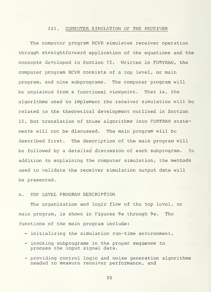
III. COMPUTER SIMULATION OF THE RECEIVER 50

A. TOP LEVEL PROGRAM DESCRIPTION 50

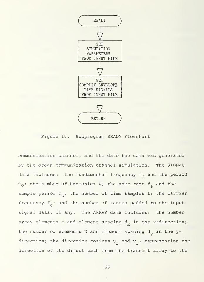
1. Subprogram READY 65

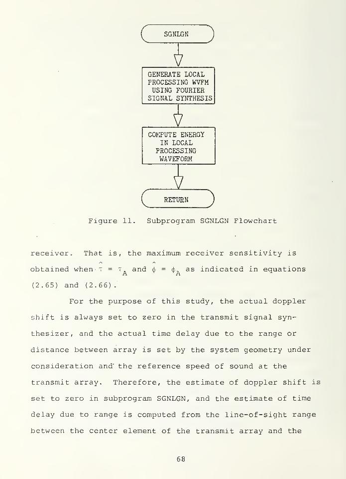
2. Subprogram SGNLGN 67

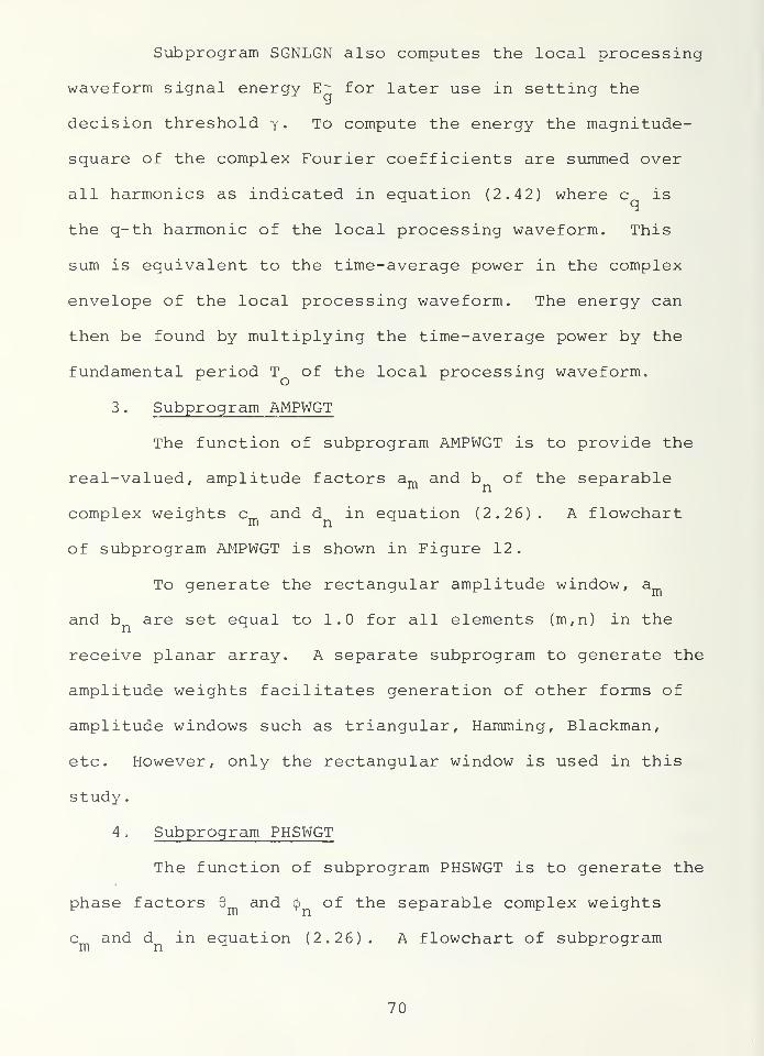
3. Subprogram AMPWGT * 70

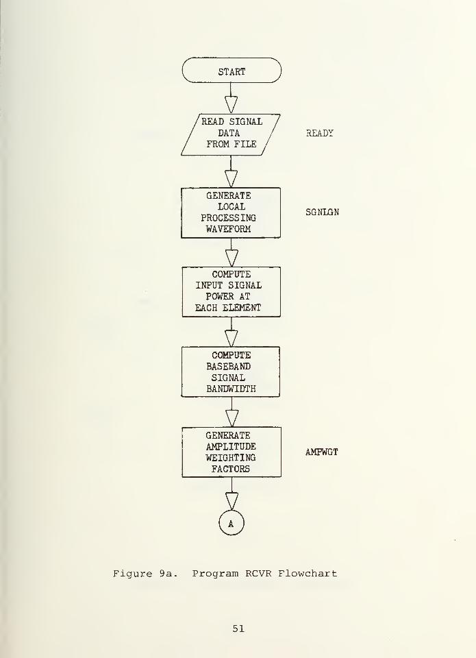
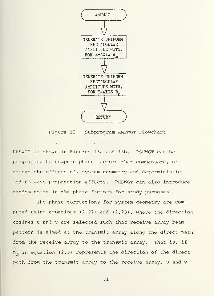
4. Subprogram PHSWGT 70

5. Subprogram ARYPRO 74

6. Subprogram AWGN 77

7. Subprogram INTGRT 79

8. Subprogram WRITBL 80

9. Subprogram PDPLOT 81

B. MODEL VERIFICATION 83

1. Characterization of the Noise Source 84

2. Verification of the Output Data 90

IV. PRESENTATION OF RESULTS 94

A. TRANSMIT WAVEFORMS 94

B. CASE TEST 98

C. CASE HMG1 107

D. CASE INHMG1 118

V. CONCLUSIONS AND RECOMMENDATIONS 134

LIST OF REFERENCES 136

INITIAL DISTRIBUTION LIST 137

LIST OF FIGURES

1. System Geometry 16

2. Ray Path Bending Due to Inhomogeneous Medium 17

3. Receiver Block Diagram 19

4. Planar Array Geometry 19

5. Array Element Quadrature Demodulator 20

6. Array Processor Block Diagram 21

7. Correlator/Matched Filter Detector 23

8. Density Functions of the Magnitude-SquareCorrelator Output 47

9. Program RCVR Flowchart 51

10. Subprogram READY Flowchart 66

11. Subprogram SGNLGN Flowchart 68

12. Subprogram AMPWGT Flowchart 71

13. Subprogram PHSWGT Flowchart 72

14. Subprogram ARYPRO Flowchart 75

15. Subprogram AWGN Flowchart 78

16. Subprogram INTGRT Flowchart — 79

17. Subprogram WRITBL Flowchart 80

18. Subprogram PDPLOT Flowchart 82

19. Histogram of I-Channel Noise 86

20. Histogram of Q-Channel Noise 87

21. Autocovariance of I-Channel Noise 88

22. Autocovariance of Q-Channel Noise 89

23. Estimated Power Spectral Density ofI-Channel Noise 91

7

24. Estimated Power Spectral Density ofQ-Channel Noise 92

25. Receiver Performance for case TEST, CW Pulse,Pfa = 0.1, Geometry Phase Weighting 101

26. Receiver Performance for case TEST, CW Pulse,Pfa = 0.01, Geometry Phase Weighting 102

27. Receiver Performance for case TEST, LFM Pulse,Pfa = 0.1, Geometry Phase Weighting 103

28. Receiver Performance for case TEST, LFM Pulse,Pfa = 0.01, Geometry Phase Weighting 104

29. Receiver Performance for case HMG1, CW Pulse,Pfa = 0.01, No Phase Weighting 109

30. Receiver Performance for case HMG1, CW Pulse,Pfa = 0.1, Geometry Phase Weighting 110

31. Receiver Performance for case HMG1, CW Pulse,Pfa = 0.01, No Phase Weighting 111

32. Receiver Performance for case HMG1, CW Pulse,Pfa = 0.01, Geometry Phase Weighting 112

33. Receiver Performance for case HMG1, LFM Pulse,Pfa = 0.1, No Phase Weighting — 113

34. Receiver Performance for case HMG1, LFM Pulse,Pfa = 0.1, Geometry Phase Weighting 114

35. Receiver Performance for case HMG1, LFM Pulse,Pfa = 0.01, No Phase Weighting 115

36. Receiver Performance for case HMG1, LFM Pulse,Pfa = 0.01, Geometry Phase Weighting 116

37. Receiver Performance for case INHMG1, CW Pulse,Pfa = 0.1, No Phase Weighting 120

38. Receiver Performance for case INHMG1, CW Pulse,Pfa = 0.1, Geometry Phase Weighting 121

39. Receiver Performance for case INHMG1, CW Pulse,Pfa = 0.1, Medium Phase Weighting —— — 122

40. Receiver Performance for case INHMG1, CW Pulse,Pfa = 0.01, No Phase Weighting — 123

41. Receiver Performance for case INHMG1, CW Pulse,Pfa = 0.01, Geometry Phase Weighting 124

42. Receiver Performance for case INHMG1, CW Pulse,Pfa = 0.01, Medium Phase Weighting 125

43. Receiver Performance for case INHMG1, LFM Pulse,Pfa = 0.1, No Phase Weighting 126

44. Receiver Performance for case INHMG1, LFM Pulse,Pfa = 0.1, Geometry Phase Weighting 127

45. Receiver Performance for case INHMG1, LFM Pulse,Pfa = 0.1, Medium Phase Weighting 128

46. Receiver Performance for case INHMG1, LFM Pulse,Pfa = 0.01, No Phase Weighting 129

47. Receiver Performance for case INHMG1, LFM Pulse,Pfa = 0.01, Geometry Phase Weighting 130

48. Receiver Performance for case INHMG1, LFM Pulse,Pfa = 0.01, Medium Phase Weighting 131

ACKNOWLEDGMENT

The author would like to thank Professor L.J. Ziomek

for his assistance, patience and encouragement during the

course of this research.

10

I. INTRODUCTION

Model-based signal processing is described by Mendel

[Ref. 1] as an approach that exploits knowledge of the

underlying physics of a problem to develop signal processing

algorithms. Use of the approach implies that some a priori

knowledge exists regarding the problem under consideration.

In the case of an underwater acoustic communication problem,

such a model has been developed by Ziomek [Ref. 2].

Ziomek derived a time-invariant, space-variant transfer

function of the ocean volume based on the WKB approximation,

which is an approximate solution of the linear, inhomogeneous

,

scalar wave equation describing the propagation of small-

amplitude acoustic pressure waves when the speed of sound is

a function of depth. Based on the transfer function of the

ocean volume, Ziomek [Ref. 2:pp. 257-261] also derived an

equation describing the output electrical signal at each

element of a planar array of point sources. The output

signal is described in terms of the frequency spectrum of

the transmitted electrical signal, the transmit and receive

planar arrays, and the random ocean medium transfer function.

Vos [Ref. 3] used these results to develop a computer program

that generates time-samples of a real baseband output

electrical signal at each element in a receive planar array

as a function of a variable ocean medium sound speed profile,

11

planar array size, array far-field beam patterns and func-

tional form of the transmit signal. Ziomek has since modi-

fied this program to generate time-samples of the complex

envelope of real bandpass output electrical signals.

The research documented in this thesis has the following

objectives

:

develop a computer simulation of a correlatorreceiver which processes the output electrical signalsgenerated by the computer program developed by Ziomekand Vos;

apply the concept of model-based signal processingto the development of the signal processing algorithmused by the receiver;

determine the effectiveness of the approach in thedetection of signals from a planar array of pointsource elements.

Since the effects of the ocean medium on the signals

processed by the receiver are embodied in the random ocean

medium transfer function, the basic question to be addressed

may be stated as follows. Can a priori knowledge of the

ocean medium, based on physical principles of acoustic wave

propagation, be used to improve the detection of signals in

a receiver, and to what degree?

Ziomek 1 s use of linear systems theory to develop a

transfer function model of the ocean medium immediately

suggests the use of a compensating filter at the array

output to remove the undesirable time delays due to system

geometry and wave propagation effects. This filter would

ideally cophase the signals at each element in the planar

array, resulting in maximum signal output when the signals

12

are added together. This filter is implemented in the

frequency domain through the use of Discrete Fourier

Transforms (DFT) , and the approach is exactly analogous to

the FFT beamforming procedure discussed by Ziomek [Ref. 2:

pp. 153-176]

.

In the frequency domain, the time delays due to system

geometry and wave propagation effects are represented as

phase shifts which may be eliminated if known a priori. The

concept of model-based signal processing is applied here to

obtain the proper compensating phase shift for the known

system geometry and wave propagation conditions.

Section II describes the theory used to develop the

receiver model. The system context within which the

receiver operates is described and related to previous

investigations. A functional description of the receiver

is shown, and each of the major functional blocks is explained

in some detail. Finally, a statistical description of the

receiver's performance is developed.

The computer implementation of the receiver structure is

described in Section III. The logical flow of the computer

program is discussed and related to the receiver descrip-

tion. The use of multiple trials to estimate the probability

of detection is explained. Each of the major subprograms

is characterized in terms of function and implementation.

Verification of the computer simulation is discussed last.

13

Section IV presents the data obtained from the simula-

tion when a rectangular-envelope, continuous wave (CW)

pulse or a rectangular-envelope, linear-frequency-modulated,

(LFM) carrier is transmitted. Receiver performance is

described by plotting the probability of detection (Pd)

,

for a given probability of false alarm (Pfa) , as a function

of the input signal-to-noise ratio (SNR) at each element

in the receive array. Plots are provided for different values

of Pfa, and show the relative improvement in receiver per-

formance as various medium and wave propagation effects

are compensated for by the model-based, signal processing

algorithm. In each plot, the receiver performance predicted

by theory when all array element output signals are precisely

cophased, and the array element .input noise is zero-mean,

uncorrelated and Gaussian is shown as a dashed line. The

dashed line is plotted from data obtained from a closed

form expression relating Pd to Pfa as a function of array

element input SNR, and is superimposed on the output plots

to provide a baseline for judging the validity of the receiver

simulation output data.

Conclusions and recommendations are discussed in

Section V.

14

II. THEORY OF THE RECEIVER MODEL

A receiver operates in the context of a total communi-

cation system consisting of a signal source (transmitter)

,

a signal propagation medium (channel) and a signal sink

(receiver) . It is the model of the communication channel

that is of initial interest since the signal processing

algorithm will depend in large part on the physics des-

cribing the propagation of the signal through the channel.

A. OVERVIEW OF THE COMMUNICATION SYSTEM

Ziomek's model (Ref. 2] of the ocean medium is described

in general as a time-variant, space-variant, random filter

(transfer function) in which the index of refraction, or

equivalently , the speed of sound, is a function of depth,

and includes both a deterministic and a random component.

However, in describing the electrical output signals from

the receive aperture, the model becomes more restrictive in

the sense that the channel is considered to be time-invariant,

but still space-variant. Furthermore, the transmit and

receive apertures are taken to be rectangular, planar arrays

whose elements consist of complex weighted point sources.

Complex weighting of the array elements provides the means

for amplitude shading and beam steering both the transmit

and receive array patterns. The complex weights are ideal

15

for removing the undesired effects of the channel on the

output electrical signals from the receive array elements,

and become the tool for applying the model-based, signal

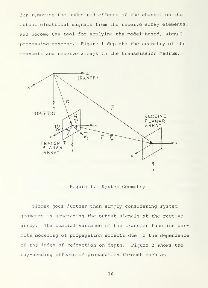
processing concept. Figure 1 depicts the geometry of the

transmit and receive arrays in the transmission medium.

TRANSMITPLANARARRAY

RECEIVEPLANARARRAY

G- 1

Figure 1. System Geometry

Ziomek goes further than simply considering system

geometry in generating the output signals at the receive

array. The spatial variance of the transfer function per-

mits modeling of propagation effects due to the dependence

of the index of refraction on depth. Figure 2 shows the

ray-bending effects of propagation through such an

16

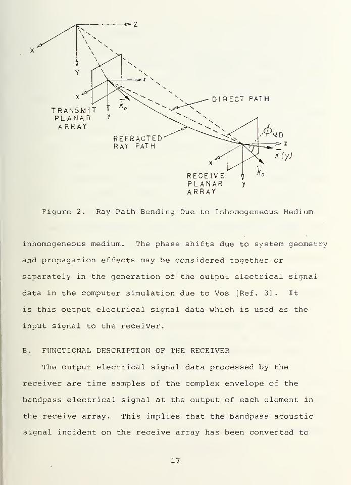
-o-Z

Dl RECT PATH

TRANSMIT VA o

PLANAR y

ARRAYREFRACTEDRAY PATH

RECEIVEPLANARARRAY

Figure 2. Ray Path Bending Due to Inhomogeneous Medium

inhomogeneous medium. The phase shifts due to system geometry

and propagation effects may be considered together or

separately in the generation of the output electrical signal

data in the computer simulation due to Vos [Ref . 3] . It

is this output electrical signal data which is used as the

input signal to the receiver.

B. FUNCTIONAL DESCRIPTION OF THE RECEIVER

The output electrical signal data processed by the

receiver are time samples of the complex envelope of the

bandpass electrical signal at the output of each element in

the receive array. This implies that the bandpass acoustic

signal incident on the receive array has been converted to

17

an output electrical signal by each transducer element in

the array. Each real, bandpass electrical signal then

passes through a quadrature demodulator to become an

equivalent baseband, complex envelope signal, which is

time-sampled and converted from analog to digital form. The

complex envelope is represented by the I-channel (in-phase)

and Q-channel (quadrature-phase) components generated by the

quadrature demodulator. Time-sampling is done in a manner

that satisfies the Nyquist criterion for the baseband infor-

mation contained in the I and Q channels. Thus, many of

the components associated with a receiving system are already

contained within the simulation that generates the planar

array output signal data. The receiver simulation assumes

these components exist, and essentially provides signal

processing of the complex envelope of the output bandpass

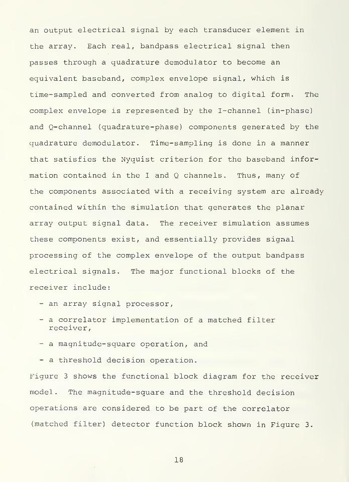
electrical signals. The major functional blocks of the

receiver include:

- an array signal processor,

- a correlator implementation of a matched filterreceiver,

- a magnitude-square operation, and

- a threshold decision operation.

Figure 3 shows the functional block diagram for the receiver

model. The magnitude-square and the threshold decision

operations are considered to be part of the correlator

(matched filter) detector function block shown in Figure 3.

PLANARA RR AY

M X NA RR AY

PROCESSOR OCORRELATORMATCHEDFILTERDETECTOR

O H,

O H

Figure 3. Receiver Block Diagram

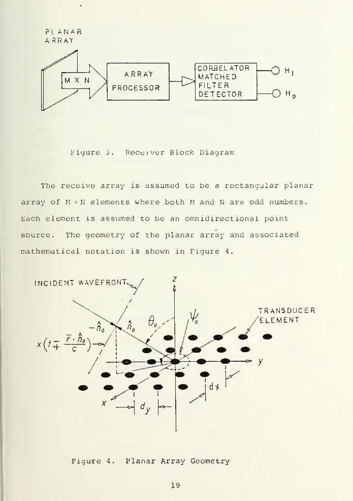
The receive array is assumed to be a rectangular planar

array of M xN elements where both M and N are odd numbers.

Each element is assumed to be an omnidirectional point

source. The geometry of the planar array and associated

mathematical notation is shown in Figure 4.

INCIDENT WAVEFRONT

TRANSDUCER/ELEMENT

y

Figure 4. Planar Array Geometry

19

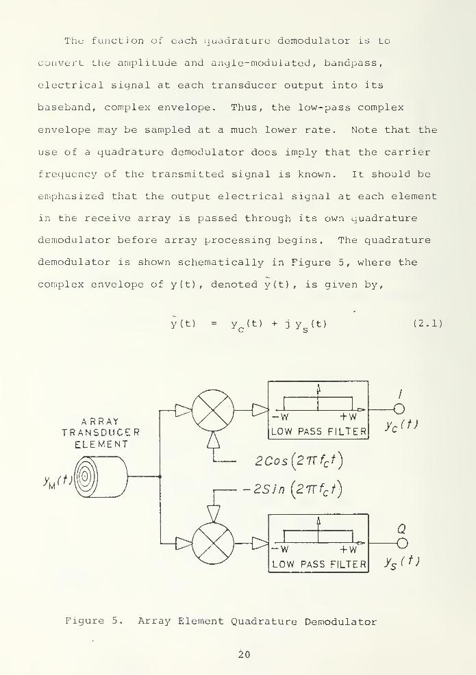
The function of each quadrature demodulator is to

convert the amplitude and angle-modulated, bandpass,

electrical signal at each transducer output into its

baseband, complex envelope. Thus, the low-pass complex

envelope may be sampled at a much lower rate. Note that the

use of a quadrature demodulator does imply that the carrier

frequency of the transmitted signal is known. It should be

emphasized that the output electrical signal at each element

in the receive array is passed through its own quadrature

demodulator before array processing begins. The quadrature

demodulator is shown schematically in Figure 5, where the

complex envelope of y(t) , denoted y(t) , is given by,

y(t) = yc(t) + j y s

(t) (2.1)

ARRAYTRANSDUCERELEMENT

2Cos(2nfc t)

2SJn (27Tfc t)

I

w +wLOW PASS FILTER

yc (t)

Q-O

y*(t)

Figure 5. Array Element Quadrature Demodulator

20

where

:

yc(t)

y s(t)

is the I-channel (in-phase) componentof y ( t) , and

is the Q-channel (quadrature-phase)component of y(t).

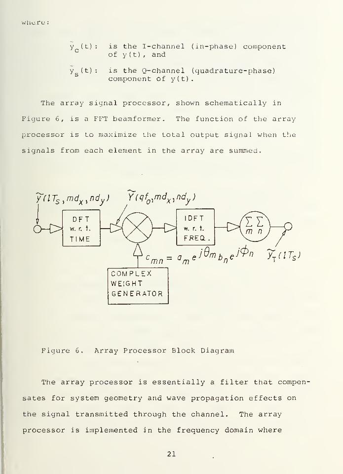
The array signal processor, shown schematically in

Figure 6, is a FFT beamformer. The function of the array

processor is to maximize the total output signal when the

signals from each element in the array are summed.

y(lTs ,mdx ,ndy) Y

r(qf ,md

x)ndy

)

(M>DFT

w. r. t.

TIME

c - a e JUm b e JVn YT (ITS )

COMPLEXWEIGHTGENERATOR

Figure 6. Array Processor Block Diagram

The array processor is essentially a filter that compen-

sates for system geometry and wave propagation effects on

the signal transmitted through the channel. The array

processor is implemented in the frequency domain where

21

filtering can be obtained by multiplication of each spectral

component of the complex envelope by a complex weighting

coefficient. The complex coefficients are computed from

a knowledge of the channel model, thus the application of

model-based signal processing. After applying the complex

weights, the Inverse DFT is computed to recover cophased,

time domain, complex envelope signals from each array ele-

ment. By summing these cophased signals over all MxM array

elements, a constructive interference effect is achieved,

and the total output signal is maximized.

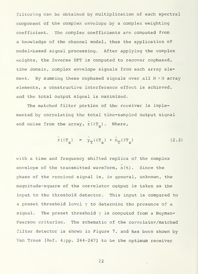
The matched filter portion of the receiver is imple-

mented by correlating the total time-sampled output signal

and noise from the array, r(£T ). Where,s

r(£T ) = yÛT ) + n_UT ) (2.2)s is is

with a time and frequency shifted replica of the complex

envelope of the transmitted waveform, x(t). Since the

phase of the received signal is, in general, unknown, the

magnitude-square of the correlator output is taken as the

input to the threshold detector. This input is compared to

a preset threshold level y to determine the presence of a

signal. The preset threshold y is computed from a Neyman-

Pearson criterion. The schematic of the correlator/matched

filter detector is shown in Figure 7, and has been shown by

Van Trees [Ref. 4:pp. 244-247] to be the optimum receiver

22

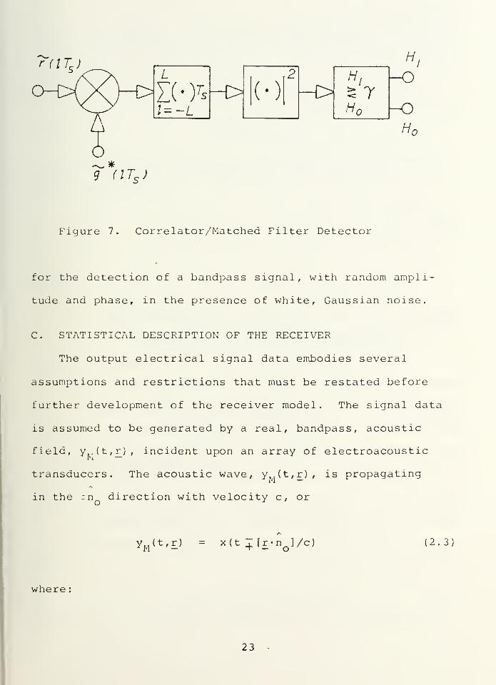
-t>

H

-o

-oHn

9 (ITS )

Figure 7. Correlator/Matched Filter Detector

for the detection of a bandpass signal, with random ampli-

tude and phase, in the presence of white, Gaussian noise.

C. STATISTICAL DESCRIPTION OF THE RECEIVER

The output electrical signal data embodies several

assumptions and restrictions that must be restated before

further development of the receiver model. The signal data

is assumed to be generated by a real, bandpass, acoustic

field, y.-(t,r) , incident upon an array of electroacoustic

transducers. The acoustic wave, y (t,r), is propagating

in the +n direction with velocity c, oro J

yM (t,r) = x(t + [£-no]/c) (2.3)

where

;

23

/\ /\

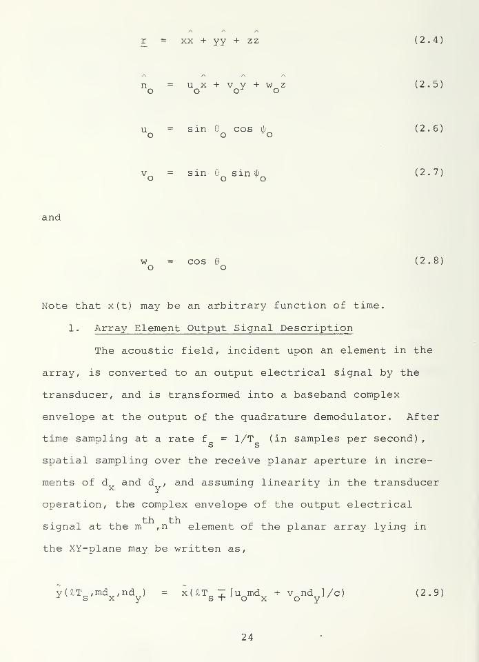
r = xx + yy + zz (2.4)

n = ux+vy+wz (2.5)o o o o

u = sin 6 cos \b (2.6)o o o

v = sin 6 sin \b (2.7)o o o

and

w = cos B (2.8)o o

Note that x(t) may be an arbitrary function of time.

1 . Array Element Output Signal Description

The acoustic field, incident upon an element in the

array, is converted to an output electrical signal by the

transducer, and is transformed into a baseband complex

envelope at the output of the quadrature demodulator. After

time sampling at a rate f = 1/T (in samples per second)

,

spatial sampling over the receive planar aperture in incre-

ments of d and d , and assuming linearity in the transducerx y 3 J

operation, the complex envelope of the output electrical

signal at the m ,n element of the planar array lying in

the XY-plane may be written as,

yUTs,md

x,nd

y) = xUT

g + [uQmd

x+ v

Qnd ]/c) (2.9)

24

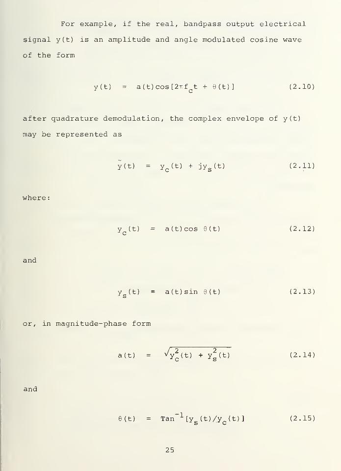
For example, if the real, bandpass output electrical

signal y(t) is an amplitude and angle modulated cosine wave

of the form

y(t) = a(t)cos[27Tf t + 6 (t) ] (2.10)

after quadrature demodulation, the complex envelope of y(t)

may be represented as

y(t) = yc(t) + jys (t) (2.11)

where

:

y (t) = a(t)cos 0(t) (2.12)c

and

y (t) = a(t)sin 6(t) (2.13)-1 s

or, in magnitude-phase form

t) = ^yl(t) + vlit]y"(t) + y c (t) (2.14)

and

(t) = Tan 1[ys

(t)/yc(t)] (2.15)

25

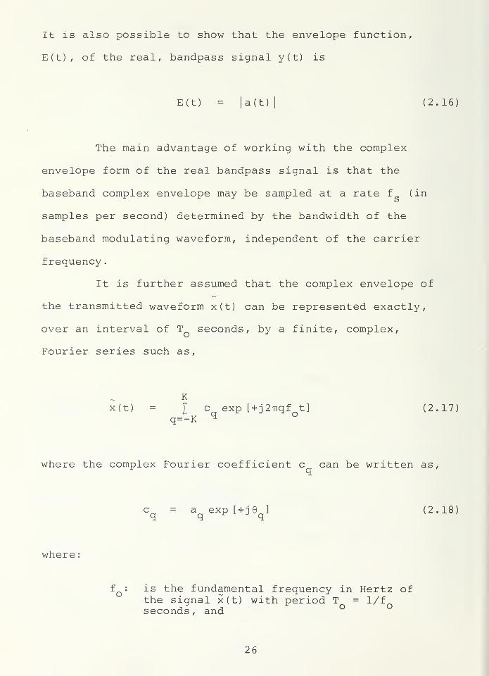
It is also possible to show that the envelope function,

E(t), of the real, bandpass signal y(t) is

E(t) = |a(t)

|

(2.16)

The main advantage of working with the complex

envelope form of the real bandpass signal is that the

baseband complex envelope may be sampled at a rate f (in

samples per second) determined by the bandwidth of the

baseband modulating waveform, independent of the carrier

frequency

.

It is further assumed that the complex envelope of

the transmitted waveform x(t) can be represented exactly,

over an interval of T seconds, by a finite, complex,

Fourier series such as,

Kx(t) =

I exp [ + j27rqf t] (2.17)q=-K q

where the complex Fourier coefficient c can be written as,q

c = a exp [+j6 ] (2.18)q q q

where

f : is the fundamental frequency in Hertz ofthe signal x(t) with period T = l/fQseconds , and

26

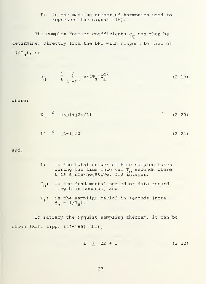
K: is the maximum number ôf harmonics used torepresent the signal x(t)

.

The complex Fourier coefficients c can then beq

determined directly from the DFT with respect to time of

x(£T ) , or

T •

cM = T J x(£T c )W^ (2.19)£=-Lq L 0__T •

S L

where

WT= exp[ + j2-^/L] (2.20)

J_l

L' = (L-D/2 (2.21)

and

L: is the total number of time samples takenduring the time interval T seconds whereL is a non-negative, odd integer,

T : is the fundamental period or data recordlength in seconds, and

o

T : is the sampling period in seconds (notefs

= 1/TS )

•

To satisfy the Nyquist sampling theorem, it can be

shown [Ref. 2:pp. 164-165] that,

L > 2K + 1 (2.22)

27

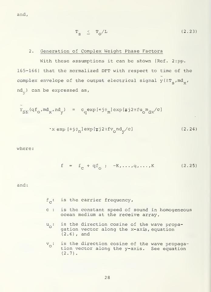
and,

T < T /L (2.23)s — o /

2 . Generation of Complex Weight Phase Factors

With these assumptions it can be shown [Ref. 2:pp.

165-166] that the normalized DFT with respect to time of the

complex envelope of the output electrical signal y(£T ,md ,

nd ) can be expressed as,

Y^ (qf ,md , nd ) = c exp[ + je ]exp[xj2Tifu m.,/c]

SN o x y q m r tJ o dx /

where

:

and

:

x exp [ + jc|)n]exp[^j27rfv

ond /cj (2.24)

f = fc

+ qfQ ; -K, . .

.

,q,. . . ,K (2.25!

f : is the carrier frequency,

c : is the constant speed of sound in homogeneousocean medium at the receive array,

u : is the direction cosine of the wave propa-gation vector along the x-axis, equation(2.6) , and

v : is the direction cosine of the wave propaga-tion vector along the y-axis. See equation(2.7)

.

28

Phase factors and <b are due to the separablem T n ^

complex weight, c . That is,r 3 mn

c „ = c d a exp[ + j6 ]b exp[ + jd) ] (2.26)mn mn m ^ J m n ^ J Tn

Notice that by a proper choice of 6 and <p in equation

(2.24) where,

) = ±j2TTfu md /c (2.27)m J o x

and

) = ±j27rfv nd /c (2.28)n J o y

the phase shifts due to system geometry may be completely

cancelled leaving only the complex Fourier coefficients c

at each element in the planar array. It should be noted

that the phase correction factors are functions of both the

array element position (mdx or ndy) , and the frequency f of

each spectral component of the input bandpass signal spec-

trum. That is, the frequency is given by equation (2.25).

Once the phase shifts due to geometry are eliminated,

taking the inverse DFT with respect to frequency of the

spectrum of the output electrical signal Y(qf ,md ,nd )

will yield cophased time signals at each element. Summing

all the cophased signals will result in a maximum total

29

output signal y (£T ) from the array processor. That

is,

M ' N

'

y (£T ) =I I yUT ,md ,nd ) (2.29)

m=-M' n=-N' y

where

M 1 = (M-D/2 (2.30)

and

N' = (N-D/2 (2.31)

This approach is extended to compensate for the

deterministic signal phase shifts caused by transmission

through an inhomogeneous ocean medium. Since the variation

in the speed of sound c(y) is assumed to be a function of y

(depth) alone, the calculation involves only the 4> phase

factor of the complex weight. Ziomek has shown that for a

sound-speed profile c(y) with a constant gradient g, a

closed form expression for the deterministic component of

phase shift is,

k c

*MD = +2^T-

{f [nD (Y)

~ 1J + AYn } (2 - 32)o ^

Extension of work by Ziomek based on expression for 6

[Ref . 2:pp. 263-268]

.

MD

30

where

nD (y) = c

o/c

D (y) (2.33)

CD (y) = cq

+ gAyn

(2.34)

A y = (y -y ) + nd (2.35)J n 2 r J o y

kQ

= 2ufQ/c (2.36)

n (y) : is the space-variant (with depth only)index of refraction,

c D (y) : is the speed of sound at depth y,

c : is the speed of sound at the transmitarray,

k : is the wave propagation constant atthe transmit array,

g : is the gradient (slope) of the soundspeed profile,

y : is the depth of the center element ofthe transmit array, and

y : is the depth of the center element of thereceive array.

The negative of the deterministic medium phase

factor, equation (2.32), is simply added to the system

geometry phase factor, equation (2.28) , to obtain the total

complex weight phase factor in the y direction.

31

3 . Array Processor Output Signal Statistics

Development of a receiver model also requires a

specification of the noise environment in which the receiver

operates. Any realistic model for the noise environment is

extremely complex. However in order to form tractable

theoretical results that can be reasonably approximated in

a computer simulation, zero-mean, additive, white, Gaussian

noise (AWGN) is assumed at the output of each array element.

Remember that the array element output is also the input to

the quadrature demodulator.

The AWGN model permits derivation of a closed form

expression relating Pd, Pfa and array input Signal-to-

Noise Ratio (SNR) . This type of noise process can also be

reasonably approximated by using computer generated pseudo-

random number sequences from a standard Gaussian random

number generator. By comparing the theoretically predicted

receiver performance with the results of the simulation,

verification of the computer implementation of the receiver

can be achieved. Once verified, the computer simulation

can test more realistic noise models with some confidence

in the resulting data.

The input SNR at a single element in the array is

defined as,

E{ |y(£T ,md ,nd) | }

SNRi

= - - ^J" (2.37)

E{ |nUT ,md ,nd ) | }

32

where E{ } denotes the expected value of the quantity within

the curly braces.

If the random input signal y ( £T ,mdr,nd ) is ergodic,

S X y

then the mean-square value of the signal can be found by

computing the time-average instead of the ensemble average,,

that is,

,2 ,

~ ,2E{ y(£T ,md ,nd ) } = < y ( £T ,md , nd > (2.38

.

|J sxy' '

* s x y '

where < (•

) > denotes the time-average of the quantity within

the parenthesis, or

T /2l °

<(•)> = sr- / C) dt (2.39)

°" T

o/2

The integral in equation (2.39) can be approximated

for computer simulation purposes by,

1L '

<(•)> = ^ I (-)T (2.40)o =-L*

where the infinitesimal dt is approximated by,

dt = Ts

(2.41)

33

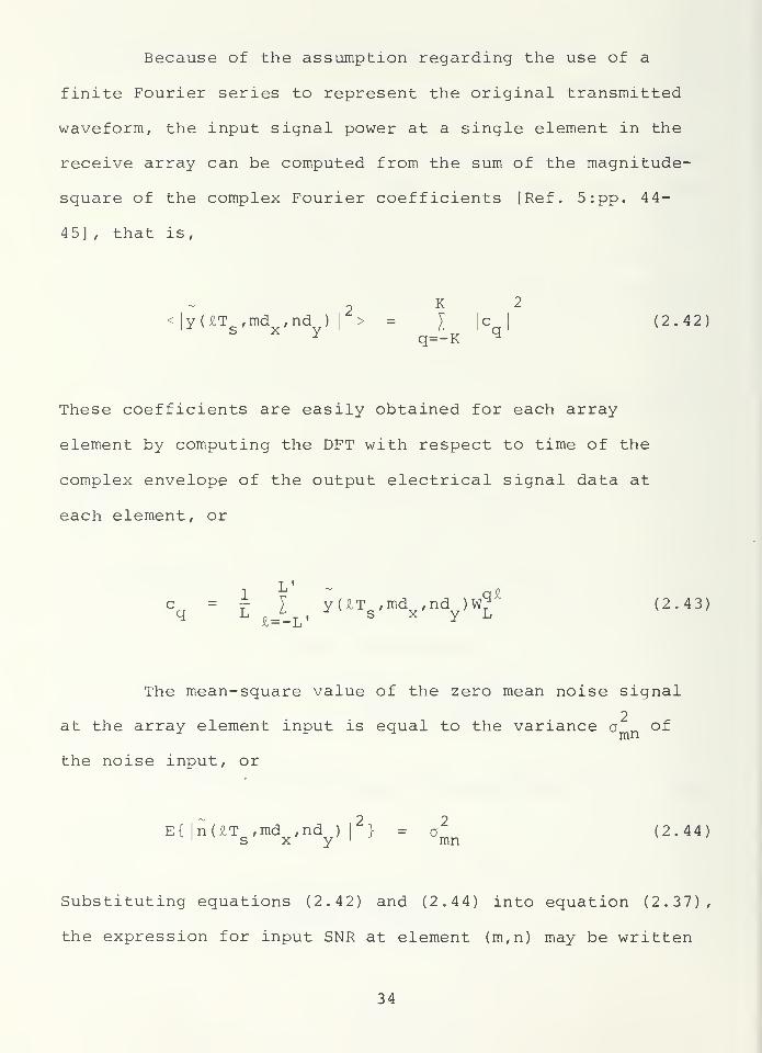
Because of the assumption regarding the use of a

finite Fourier series to represent the original transmitted

waveform, the input signal power at a single element in the

receive array can be computed from the sum of the magnitude-

square of the complex Fourier coefficients [Ref. 5:pp. 44-

45] , that is,

2 K 2

<|yUT ,md ,nd ) I> = Y |c I (2.42)

1 2 s x y ' ' , ' q

'

J q=-K ^

These coefficients are easily obtained for each array

element by computing the DFT with respect to time of the

complex envelope of the output electrical signal data at

each element, or

L

'

c = ^ 7 y(£T ,md ,nd )W?£

(2.43)q L isiL ,

y s x' y L

The mean-square value of the zero mean noise signal

2at the array element input is equal to the variance o of

the noise input, or

E{|n(£T ,md ,nd )|2

} = q2

(2.44)1 s x y ' mn

Substituting equations (2.42) and (2.44) into equation (2.37),

the expression for input SNR at element (m,n) may be written

34

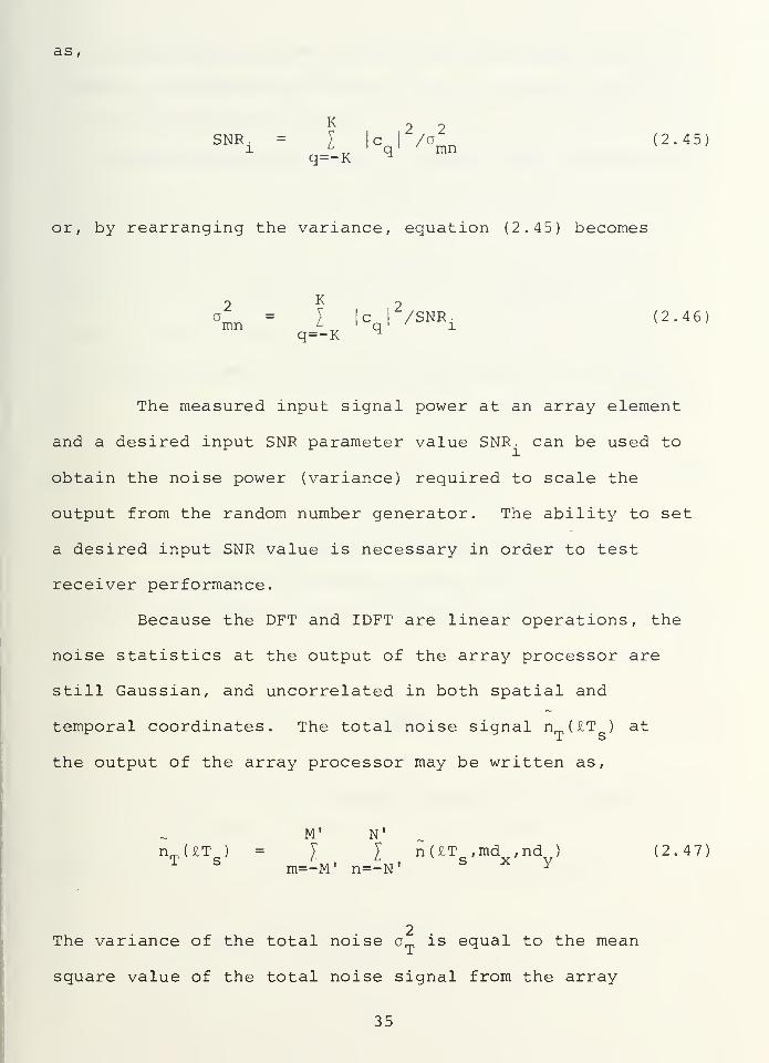
as,

SNR. 7 |c|

2/o

2(2.45)

1 L_,

' q'

' ranq=-K ^

or, by rearranging the variance, equation (2.45) becomes

a2

7 |c|

2/SNR. (2.46mn L

, ' q ' ' lq=-K ^

The measured input signal power at an array element

and a desired input SNR parameter value SNR. can be used to

obtain the noise power (variance) required to scale the

output from the random number generator. The ability to set

a desired input SNR value is necessary in order to test

receiver performance.

Because the DFT and IDFT are linear operations, the

noise statistics at the output of the array processor are

still Gaussian, and uncorrelated in both spatial and

temporal coordinates. The total noise signal nm ( £T ) atJ T s

the output of the array processor may be written as,

M 1 N 1

nTUT

s) = I I nUT

s,md

x,nd ) (2.47)

m=-M' n=-N'

2 .

The variance of the total noise o_ is equal to the mean

square value of the total noise signal from the array

35

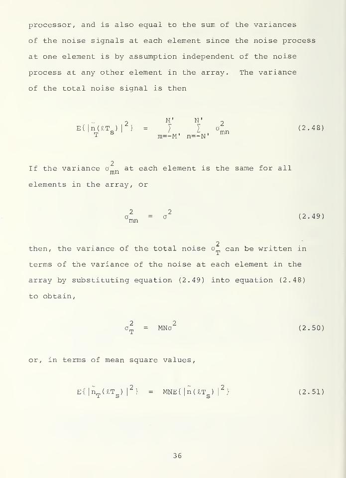
processor, and is also equal to the sum of the variances

of the noise signals at each element since the noise process

at one element is by assumption independent of the noise

process at any other element in the array. The variance

of the total noise signal is then

E{|nUTs )|

2) = J I omn (2.48)

1 m=-M' n=-N'

2If the variance a „ at each element is the same for allmn

elements in the array, or

a2

= a2

(2.49)mn

2then, the variance of the total noise a can be written in

terms of the variance of the noise at each element in the

array by substituting equation (2.49) into equation (2.48)

to obtain,

a2

= MNo2

(2.50)

or, in terms of mean square values,

E{ |nrT,(£T c )

|

2} = MNE{ |n(£T o )

|

2} (2.51)

1 o S

36

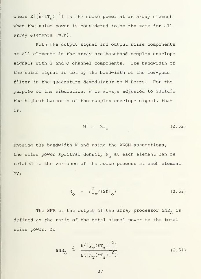
i

2where E{ n(£T ) } is the noise power at an array element

when the noise power is considered to be the same for all

array elements (m,n).

Both the output signal and output noise components

at all elements in the array are baseband complex envelope

signals with I and Q channel components. The bandwidth of

the noise signal is set by the bandwidth of the low-pass

filter in the quadrature demodulator to W Hertz. For the

purpose of the simulation, W is always adjusted to include

the highest harmonic of the complex envelope signal, that

is,

W = KfQ

(2.52)

Knowing the bandwidth W and using the AWGN assumptions,

the noise power spectral density N at each element can be

related to the variance of the noise process at each element

by,

N = ai/(2Kf ) (2.53)o mn o

The SNR at the output of the array processor SNR is

defined as the ratio of the total signal power to the total

noise power, or

AE{|y (£T

)

|

2}

SNR a= ^ j- (2.54)

AE(|n UT )

|

Z}

37

where,

2M' N 1

2E{|yT UT )| } = E{| I I yUT ,md ,nd )

|} (2.55)

1 Sm=-M' n=-N' s x y

For the case of perfectly cophased signals with identical

signal power at each element, the right-hand side of equa-

tion (2.55) reduces to

E{ |yT(£T

s)

|

2} = (MN)

2E{ |y(£T

s )

|

2} (2.56)

i

2where E{[y(£T

) |} is equivalent to the time-average power

i 2at each element in the array, and E{|y (£T) | } is equivalent

J. O

to the time-average power of the total output signal from

the array processor. Using the uncorrelated and equal

array element input power noise assumptions, the expression

for SNR can be rewritten by substituting equations (2.51)

and (2.56) into equation (2.54), or

E{ |yUT )|

}

SNR = MN 5— = MNSNR. . (2.57)A E{|nUT )\

}

X

Since the array gain (AG) is defined as,

AG = 10 log [SNRA/SNR d] (dB) (2.58)

38

the array gain in this case becomes,

AG = 10 log [MN] (dB) (2.59

Note that for a 5 x 5 element planar array, M *N = 25, and

the array gain is 13.979 dB

.

4 . Hypothesis Testing and the Neyman-Pearson Criterion

The correlator/matched filter detector portion of

the receiver, Figure 7, is modeled as a binary hypothesis

testing problem using the Neyman-Pearson decision criterion.

The two hypotheses, H and H, , are defined as,

I V £V + nT

U

£T ) : H,s 1

IT )

T(£T

s) : H

q

where, in terms of the transmitted waveform x(t),

M' N 1

y (IT > = c I I x K«s-V),^,nd]

m=-M' n=-N' 2

x exp [ + j2TT(f)2,ilT J (2.61)A s

and n (£T ) is given by equation (2.47). If one assumesJ. O

that all array element output signals are cophased and

identical, equation (2.61) reduces to

39

y (£T ) = cMNxUT -t ) exp [ + j 2 tt 4> a £T ] (2.62)

where

:

and,

'A

c = a exp [+j6] (2.63)

t : is the actual time delay in seconds ateach element in the array due to rangeseparation between individual elementsof the transmit and receive arrays,

t a: is the actual time delay in seconds due

to range separation between transmitand receive arrays when all signals arecophased,

is the actual doppler shift in Hertz dueto relative motion between transmit andreceive arrays,

a: is the amplitude attenuation factor thatis, in general, a random variable,

6: is the generalized phase shift of thereceived signal with respect to the trans-mitted signal. (In general, it is also arandom variable dependent on both spatialand temporal coordinates.), and

Hq : is the null or noise only (no signal)hypothesis

.

Matched filtering is obtained by correlating the

complex envelope of the total array output r(£T ) with the

complex conjugate of the processing waveform g(£T ). The

functional form of g ( £T ) can be written as,

g(£T ) = x(£T -T)exp[ + j27Tcf)£T J (2.64)o S S

40

which is a time and frequency shifted replica of the

transmitted signal x(t) where

t : is the estimate of time delay at the receiver,and

$ : is the estimate of the doppler shift at thereceiver.

For the purposes of this study, the estimates of

time delay and doppler shift are assumed to be precisely

correct, or

x = t - t_ = 0.0 (2.65)A

and

$ = <j>-

<f>= 0.0 (2.66)

The correlation, or inner product I between two

functions r(t) and g(t), is given by

I = <r(t),g(t)> = / r(t)g*(t)dt (2.67)

which is approximated in the simulation using the trapezoidal

rule approximation to the integral, that is,

L'-l r(£T )g*UT ) + r[U+l)T ]g*[U+l)T_)I =

I= — T (2.68)

JL=-L'S

41

The magnitude-square of the correlator output is

taken for two reasons. First, the phase of the carrier

frequency waveform is, in general, unknown. As the phase

of the received carrier varies with respect to the phase of

the quadrature demodulator local oscillator (LO) signal, the

output of the quadrature demodulator would vary from a

maximum negative to a maximum positive value depending on

the phase difference between the carrier and the LO which

usually is taken to be a uniformly distributed random varia-

ble between and 2tt radians. The change in polarity of

the quadrature demodulator output would propagate through

to the output of the integrator in the correlator/matched

filter detector, Figure 7. Taking the magnitude of the

integrator output ensures that the input to the threshold

comparator will always be non-negative regardless of the

phase difference between the carrier and LO waveforms.

Second, when the array element noise statistics are assumed

to be Gaussian, the square of the magnitude of the integrator

output yields an input to the threshold comparator which

can be described statistically by exponential density

functions for both H, and H» signal hypotheses. As will

be shown in the following derivations, the exponential den-

sity functions can be easily integrated to obtain a closed

form expression for Pd and Pfa in terms of the SNR at the

input to the threshold comparator. The output of the

magnitude-square operation is the sufficient statistic

42

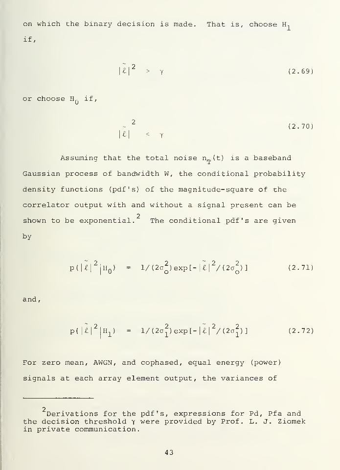
on which the binary decision is made. That is, choose H.

if,

I > y (2.69

or choose H, if,

(2.70)

Assuming that the total noise n (t) is a baseband

Gaussian process of bandwidth W, the conditional probability

density functions (pdf 's) of the magnitude-square of the

correlator output with and without a signal present can be

2shown to be exponential. The conditional pdf ' s are given

by

P(U|2|H ) = l/(2a^)exp[-U|

2/(2a^)] (2.71)

and,

P( |£ V l/(2o^)exp[-|£|2/(2a

2)] (2.72)

For zero mean, AWGN, and cophased, equal energy (power)

signals at each array element output, the variances of

Derivations for the pdf's, expressions for Pd, Pfa andthe decision threshold y were provided by Prof. L. J. Ziomekin private communication.

43

the magnitude-square of the correlator output can be shown

to be

where

o= E{ \l

N}/2 MNN EV2 (2.73)

and

°1 = E{|£s |

2+ KN |

2)/2

[ (MN) E(a } X(t,4>) I

2+ MNN E~]/2

o X(2.74)

I.|

: is the magnitude-square of the correla-tor output when the input to thereceive array is noise alone,

is the magnitude square of the correla-tor output when the input to receivearray consists of signal alone,

No

X

E(a^} :

is the power spectral density level ofthe noise signal at each array elementoutput,

is the energy in the transmitted signalwhich for simulation purposes is definedto be equal to the energy E~ in the localprocessing waveform g(t),

is the mean-square value of the amplitudeattentuation factor (note: E{a } = a2only when deterministic effects areconsidered) , and

X(x,<j>) is the magnitude-square of the auto-ambiguity function. Note that |X((x,d>) |2

Et|X (t , 4>)

I

z, or in our case where t =

and cf)= 0, |X(0,0)| 2 = E? since

XN (0,0) |2 = 1. [Ref. 2:pp. 190-191]

44

To calculate the threhold y for a desired Pfa and

input SNR, the integral of the pdf for the null, or H

hypothesis, is set equal to the desired Pfa, and the result-

ing equation is solved for the threshold. The magnitude-

square operation results in particularly simple threshold

equation when the input noise is assumed to be white, zero

mean, and Gaussian. Computing the Pfa yields

+00

Pfa / P( \l I

2H n

)d|£

|

2

Y

= exp[-y/(2oQ )

]

= exp[-y/(MNN E-~) ]O X(2.75)

By solving equation (2.75) for the threshold y,

y = MNN E~ in [1/Pfa]U 2\.

(2.76)

Once the threshold is obtained, the correlator

output pdf for the H-, hypothesis may be evaluated to obtain

the Pd.

Pd = / p(K E±)d\l

= exp[-y/2a1

]

exp{-y/[ (MN)2E{a}

2X(t,<J>)

|

2+MNN E~}J

45

(2.77)

Since in our problem t = and § = ,

X(x,<t>) I

2= |X(0,0)

I

2= E? (2.78)

x

and if we let

E{a2}E~

SNR|^,2 = MN( -) (2.79)

then,

MNE{a2}E~

Pd = exp{-y/[MNN E~ (= + 1)]} (2.80)r O X No

and

Pd = exp{-y/[MNN E~(SNR,-|2 + 1)J} (2.81)ox\ Jt

\

Substitution of equation (2.75) into equation (2.81)

gives the desired closed form expression relating Pd, Pfa

and the SNR of the magnitude-square of the correlator output,

that is,

1/U+SNR, t; ,2]

Pd = Pfa '

' (2.82)

This result agrees in form with the result given in Van

Trees [Ref. 4:pp. 246-247] for a similar single channel

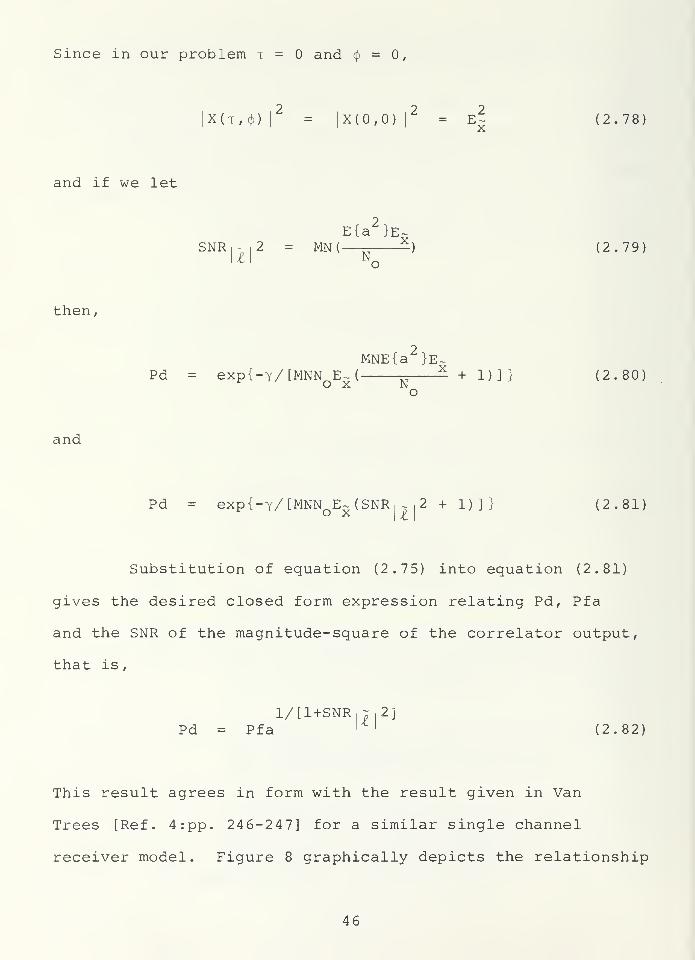
receiver model. Figure 8 graphically depicts the relationship

46

2p(\T\ Ho)

p(\lf\",)

THRESHOLDA Pfa

I

2

Figure 8. Density Functions of the Magnitude-Sqaure Correlator Output

between the conditional pdf's, the decision threshold y, the

Pfa and the Pd.

The correlator output SNR, equation (2.79), can be

related to the input SNR at a single element in the array

through the array gain, and a factor resulting from the

slightly different definitions of input SNR and correlator

output SNR. In terms of array element input signal energy

E - , the input SNR given in equation (2.45) may be rewritten

as,

SNR.l

1/T )E~° y

mn

E{a }E~x

T a „o mn

(2.83)

47

where

,

E~ = E{a2}E

x(2.84)

is the average received energy at a single element in the

array due to the transmitted signal x(t), and from equation

(2.53)

72kN

o „ = 2kf N = —-2. (2.85)ran o o T

o

The magnitude-square correlator output SNR can be written

as

,

SNR,^,2 = _s

_- (2.86)£

l Ed^l2

)

where,

E{\1\

A} = (MN)

2 E{a2}E- (2.87)

and,

E{|AJ 2} = MNNE; (2.88)

Substitution of equations (2.87) and (2.88) into equation

(2.86) gives

48

E{a2}E-

SNR|~,2 = MN - (2.89)\t\

By substituting equation (2.85) into equation (2.83) and

rearranging terms, equation (2.83) becomes

E{a2}E-

SNRi

=2KN

X(2 - 90

o

By rearranging terms in equation (2.90) and substituting

the result into equation (2.89), the desired relationship

expressing the magnitude-square correlator output SNR in

terms of the array element input SNR at a single element

in the array is obtained. That is,

SNR, ^,2 = MN2KSNR. (2.91)

Writing both sides of equation (2.91) in dB form yields,

SNR, ^ I 2 (dB) = 10 1og10

(MN) + 10 1og(2K) + SNR. (dB)

(2 92AG [

where AG is the array gain given in equation (2.59).

To summarize, Section II. C provides the equations

needed to implement a computer simulation of the receiver

structure described in Section II. B. The implementation of

the computer simulation is the subject of Section III.

49

Ill . COMPUTER SIMULATION OF THE RECEIVER

The computer program RCVR simulates receiver operation

through straightforward application of the equations and the

concepts developed in Section II. Written in FORTRAN, the

computer program RCVR consists of a top level, or main

program, and nine subprograms. The computer program will

be explained from a functional viewpoint. That is, the

algorithms used to implement the receiver simulation will be

related to the theoretical development outlined in Section

II, but translation of these algorithms into FORTRAN state-

ments will not be discussed. The main program will be

described first. The description of the main program will

be followed by a detailed discussion of each subprogram. In

addition to explaining the computer simulation, the methods

used to validate the receiver simulation output data will

be presented.

A. TOP LEVEL PROGRAM DESCRIPTION

The organization and logic flow of the top level, or

main program, is shown in Figures 9a through 9e. The

functions of the main program include:

- initializing the simulation run-time environment,

- invoking subprograms in the proper sequence toprocess the input signal data.

- providing control logic and noise generation algorithmsneeded to measure receiver performance, and

50

START

READ SIGNALDATA

FROM FILEREADY

GENERATELOCAL

PROCESSINGWAVEFORM

SGNLGN

COMPUTEINPUT SIGNALPOWER AT

EACH ELEMENT

COMPUTEBASEBANDSIGNALBANDWIDTH

GENERATEAMPLITUDEWEIGHTINGFACTORS

AMPWGT

Figure 9a. Program RCVR Flowchart

51

&GENERATEPHASE

WEIGHTINGFACTORS

PHSWGT

COMBINE A, B,

THETA, PHITO GENERATECOMPLEX WGT.

GENERATETOTAL ARRAYOUTPUT SIGNAL

ARYPRO

COMPUTEENERGY IN

OUTPUT SIGNAL

COMPUTE SNRSTEP ANDNUMBER OF

TRIALS (NRUNS)

Figure 9b. Program RCVR Flowchart

52

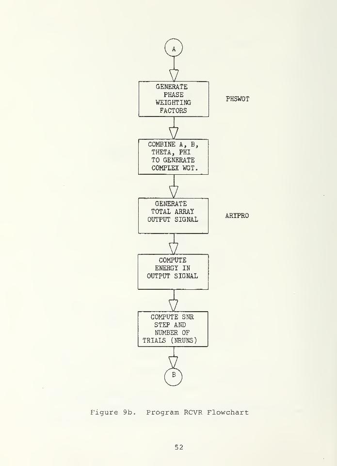
SNR - SNR+SNRSTP

ZCOMPUTE

ESTIMATEOF Pfa

5"

COMPUTEESTIMATE

OF Pd

5"

COMPUTENOISE VARIANCEAT EACH ARRAY

ELEMENT

COMPUTETOTAL NOISE

VARIANCE ANDPWR SPECTRAL DEN.

COMPUTEARRAY OUTPUT

SNR ANDARRAY GAIN

COMPUTEDETECTIONTHRESHOLD

Figure 9c. Program RCVR Flowchart

53

A

€

©

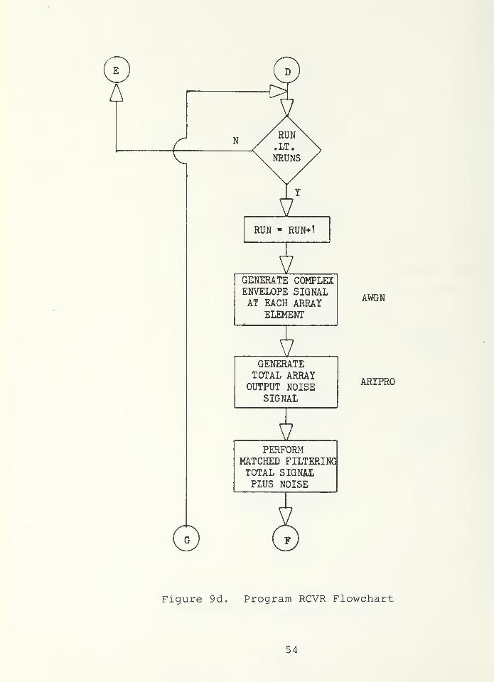
RUN - RUN+1

GENERATE COMPLEXENVELOPE SIGNALAT EACH ARRAY

ELEMENT

GENERATETOTAL ARRAYOUTPUT NOISE

SIGNAL

PERFORMMATCHED FILTERINGTOTAL SIGNALPLUS NOISE

AWGN

ARYPRO

Figure 9d. Program RCVR Flowchart

54

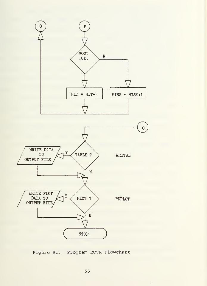
G

A

N

HIT = HIT+1

5MISS - MISS+1

/ WRITE DATATO

OUTPUT FILE

WRITE PLOTDATA TO

OUTPUT FILEPDPLOT

Figure 9e. Program RCVR Flowchart

55

- selecting the form of the simulation output data.

Initialization of the run-time environment involves reading

input data from file to internal storage, generating the

local processing waveform, measuring the time-average input

signal power at each array element, computing the baseband

signal bandwidth, and generating the complex weights used

by the array processor. The input data is read by a call

to the subprogram READY which returns a set of simulation

parameters in COMMON storage and the complex envelope

electrical signal data for each array element in matrix

form. The local processing waveform is obtained by a call

to the subprogram SGNLGN. The time-average signal power

at each element (m,n) in the planar array is found by using .

the fact that the original transmit signal was synthesized

from a finite Fourier series, and applying equation (2.43)

to obtain the complex Fourier coefficients, c . Once the

complex Fourier coefficients at each element in the planar

array are obtained, the time-average power is computed using

equation (2.42). The baseband signal bandwidth W is com-

puted using equation (2.52). The separable complex weights,

cm and d inequation (2.26) are generated in two stages.

First, the real amplitude factors, am and b in equation

(2.26), are computed by a call to subprogram AMPWGT. Second,

the real phase factors, 9 and <p in equation (2.26), are

obtained by a call to subprogram PHSWGT. The complex weights

are then computed by combining the amplitude and phase

factors as shown in equation (2.26).

56

The first signal processing step is to generate the

total array output signal in the absence of additive noise

by a call to subprogram ARYPRO. Subprogram ARYPRO which

uses the complex weights c and d to cophase the planar

array output signal returns a total array output signals.

The total array output signal energy is computed using

equation (2.40) for later use in calculating a SNR at the

output of the array processor. The ratio of array output

SNR to the input SNR defines the array gain, and provides a

check on the validity of the data generated by the array

processor algorithm.

Receiver performance is measured by computing a relative

frequency estimate of the Pd over the specified range of

array element input SNR values when the Pfa is a known,

time- invariant parameter. Using the Pfa and a range of SNR

values specified by the programmer in a receiver control

data block, the main program establishes nine input SNR

values for which the estimate of the Pd will be computed,

and determines the number of trials, or runs, to be used in

computing the estimate.

At point B in the flowchart of Figure 9c, the main

program enters a loop that initializes the noise source,

performs an array gain calculation, computes the detection

threshold and then enters a second, inner loop where the

correlation detection is done. After exiting the inner

loop, the relative frequency estimate of the Pd is computed.

57

The outer loop increments through the input SNR values

determined earlier, and exits the loop when the specified

maximum input SNR value is reached.

The first step in initializing the noise generator is

to determine the noise variance (power) at each array element.

The power level, or variance, of the noise samples for a

particular element in the array is a function of the time-

average signal power at each element and the array element

input SNR. The variance can be found using equation (2.46).

By controlling the power level of the noise process at

each array element, the receiver performance can be measured

over a range of array element input SNR values regardless

of the time-average signal power level at a particular

array element.

The variance computed in this manner is the variance of

the complex envelope baseband noise signal. The variance of

the real baseband noise signal produced by the noise generator

subprogram AWGN in the I or Q channel is one-half the vari-

ance of the complex noise signal since the complex envelope

is the sum of the two independent I and Q channel noise sig-

nals. Therefore, the variance of the complex envelope of

the noise is divided in half prior to being passed to the

noise generating subprogram as a scale parameter.

The variance of the total complex envelope noise signal

2a is obtained by summing all the noise variances of the

2array element complex envelope signals, a , as indicated

58

by equation (2.48). A power spectral density of the total

2noise signal is computed using equation (2.53) where o is

2substituted for omn

The SNR at the array processor output is computed using

equation (2.54) where the time-average power of the total

array output signal is substituted for the mean square

ensemble average, and the mean square ensemble average of

the total noise is taken to be the same as the total noise

signal variance. The array gain is computed using equation

(2.58), and is held in internal storage for later output in

tabular format.

The detection threshold y is computed using equation

(2.76) where the total noise power spectral density is

substituted for the MNN factor and the energy of the localo ^ J

processing waveform E~ is used instead of the transmit^g

signal energy E~ . For the purpose of this simulation however,

the energy in the local processing waveform is the same as

the energy in the transmit waveform. That is, E~ and E~

are equal.

The second, or inner loop, of the main program begins

at point D in Figure 9c. Within the inner loop, the complex

envelope noise signals are generated for all array elements,

the total noise output signal is generated by the array

processor subprogram ARYPRO, the total signal and total

noise are summed and correlated with the local processing

waveform, and the signal detection decision is made. The

59

inner loop terminates when the number of iterations through

the loop equals the number of trials allowed to form the

estimate of Pd.

The time-sampled, complex envelope array element noise

data is obtained by repeated calls to the noise generator

subprogram AWGN. Each call to AWGN returns a properly

scaled pseudorandom number representing one sample of the

noise process in the I or Q channel at a particular array

element with L time samples taken for each of the I and Q

channels. The noise signal data is stored in the same

matrix form as the array element output electrical signal

data.

The complex envelope noise data is submitted to the

array processor subprogram for processing in exactly the

same manner as the input signal data. The result is an

array total noise output signal. Processing the noise alone

in this manner provides some gain in execution speed and

provides the flexibility to estimate the probability of

false alarm directly, if desired. The DFT and IDFT are

linear operations, and the principle of superposition holds.

Therefore, the addition of the total noise and total signal

at the output of the array processor is equivalent to adding

noise to the signal at each element prior to passing the

data to the array processor subprogram.

Correlation of the sum of the total signal and total

noise with the local processing waveform is accomplished by

60

using the trapezoidal rule to approximate the integral of

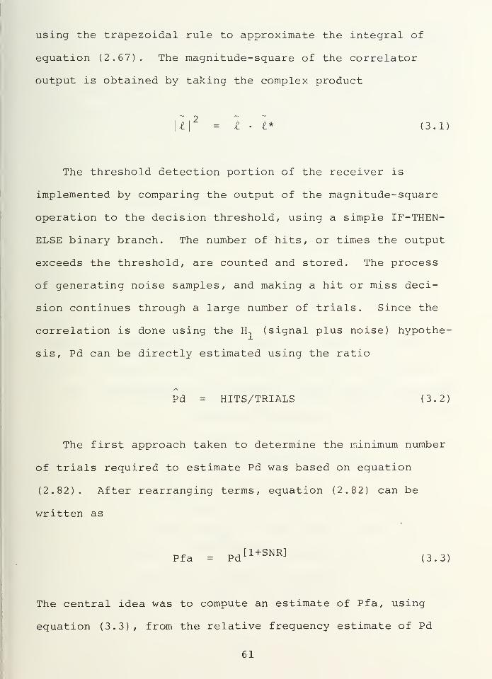
equation (2.67). The magnitude-square of the correlator

output is obtained by taking the complex product

l\2

= I • I* (3.1)

The threshold detection portion of the receiver is

implemented by comparing the output of the magnitude-square

operation to the decision threshold, using a simple IF-THEN-

ELSE binary branch. The number of hits, or times the output

exceeds the threshold, are counted and stored. The process

of generating noise samples, and making a hit or miss deci-

sion continues through a large number of trials. Since the

correlation is done using the H, (signal plus noise) hypothe-

sis, Pd can be directly estimated using the ratio

Pd = HITS/TRIALS (3.2)

The first approach taken to determine the minimum number

of trials required to estimate Pd was based on equation

(2.82). After rearranging terms, equation (2.82) can be

written as

Pfa = Pd U+SNR] (3 . 3)

The central idea was to compute an estimate of Pfa, using

equation (3.3), from the relative frequency estimate of Pd

61

in equation (3.2). The algorithm would then terminate when

the computed estimate of Pfa differed from the Pfa input

parameter by some arbitrary small amount. However, the use

of equation (3.3) was found to be a poor test for establish-

ing when the algorithm should terminate, and would not

terminate the algorithm for Pd values greater than about

0.6.

A perturbation sensitivity analysis of equation (3.3)

can be performed by computing the total differential of

equation (3.3). That is,

dpfa w dPd + fit dSNR

dPfa = [l+SNRjPdSNR

dPd + Pd[1+SNR:1

£n (Pd) dSNR (3.4)

Assuming that the SNR is a constant, or equivalently , the

differential dSNR is zero, dPfa becomes

dPfa = [l+SNR]PdSNR

dPd (3.5)

or

APfa = [l+SNR]PdSNR

APd (3.6)

where

62

dPfa * APfa = |Pfa-Pfa| (3.7)

and

dPd z APd |Pd-Pd| (3.8)

Dividing both sides of equation (3.6) by equation (3.3)

yields

APfa. = [1+SNR]APd

Pfa Pd

where APfa/Pfa and APd/Pd represent the fractional error

between the actual and estimated values of Pfa and Pd

,

respectively.

Such an analysis indicates that the percent error in the

computed estimate of Pfa is linearly related to the percent

error in the estimate of Pd. The constant of proportionality

relating the error in the computed estimate of Pfa to the

error in Pd estimate is equal to (1 + SNR) where the SNR is

taken at the output of the magnitude-square operation. Thus

for SNR values greater than approximately 1, or dB, a small

error in the relative frequency estimate of Pd is scaled to

a larger error in the estimate of Pfa found by using equation

(3.3). Note that for a 5 *5 element planar array and a

bandwidth of 5 times the fundamental frequency as in the CW

pulse case, the array element input SNR can be found by

63

equation (2.92), and is roughly 24 dB less than the SNR at

the output of the magnitude-square operation. That is, a

dB SNR at the output of the magnitude-square operation

corresponds to an array element input SNR of -24 dB . The

end result is an estimate of Pfa that diverges wildly from

the specified Pfa parameter at SNR values over which the

receiver operates. In addition, equation (3.3) was derived

using certain assumptions regarding the statistics of the

input noise that may not be precisely duplicated by the

pseudorandom noise data generated by the computer program.

If the assumptions regarding the use of zero mean, uncorre-

cted, Gaussian noise are not satisfied by the pseudorandom

noise source, equation (3.3) does not hold, and the algorithm

would not be suitable for other input noise models. For

these reasons, the use of equation (3.3) was abandoned in

favor of an empirically determined fixed number of trials to

estimate Pd.

The number of trials needed to estimate Pd was found by

assuming that the absolute minimum number of trials should

be the reciprocal of the Pfa parameter. That is, if a Pfa

of 0.01 is specified, at least 100 trials must be taken to

allow at least one chance in one hundred of a false alarm

occurring. Even though a relative frequency estimate of Pd

is being computed, Pd is related implicitly to Pfa through

the decision threshold, and the value of the Pfa parameter

should be taken into account when attempting to fix the

number of trials needed to estimate Pd.

64

The number of trials was empirically determined by

running the receiver simulation program repeatedly with

increasing multiples of the minimum number of trials, and

observing the effect on the estimate of Pd. Depending upon

the value of the Pfa parameter, it was found that four to

eight times the minimum number of trials would produce

curves that did not change appreciably as the number of

trials was increased further. Therefore, the fixed number

of trials used to estimate Pd was arbitrarily set at 10 x 1/Pfa

for Pfa of 0.1, and to 5 x.l/Pfa for Pfa of 0.01. The smaller

multiplier for the Pfa of 0.01 became necessary due to limits

on computer resources.

1. Subprogram READY

The function of subprogram READY is to obtain the

simulation parameters and the complex envelope output

electrical signal data from a data file. The data file is

generated by the ocean communications channel simulation

computer program developed by Vos and Ziomek [Ref. 3]. That

is, READY forms the interface between the RCVR simulation

and the ocean communications channel program. A flowchart

of READY is shown in Figure 10.

The simulation parameters are read in first, and

are stored in the named COMMON blocks: HEADER, SIGNAL,

ARRAY, and MEDIUM. The named COMMON blocks provide the

mechanism for communicating simulation parameters into the

various subprograms. The HEADER data documents the type of

65

READY

GETSIMULATIONPARAMETERS

FROM INPUT FILE

GETCOMPLEX ENVELOPE

TIME SIGNALSFROM INPUT FILE

4RETURN

Figure 10 . Subprogram READY Flowchart

communication channel, and the date the data was generated

by the ocean communication channel simulation. The SIGNAL

data includes: the fundamental frequency f and the period

T ; the number of harmonics K; the same rate f and the

sample period T ; the number of time samples L; the carrier

frequency f ; and the number of zeroes padded to the input

signal data, if any. The ARRAY data includes: the number

array elements M and element spacing d in the x-direction;

the number of elements N and element spacing d in the y-

direction; the direction cosines u and v , representing the

direction of the direct path from the transmit array to the

66

receive array; the direction cosines u, and v, , representing

the direction the transmit array beam pattern was steered in

the communication channel simulation; the depth y of the

center element of the transmit array; and the depth y of

the center element of the receive array. The MEDIUM data

includes the speed of sound c at the center element of the

transmit array; the sound-speed-profile gradient g; and

the speed of sound c at the center element of the receive

array.

The time-sampled, complex envelope, output electri-

cal signal data is read in next. The data is stored in the

complex matrix variable YCE with dimensions L, M and

N. The maximum values of L, M, and N are limited to 33, 11

and 11, respectively.

2. Subprogram SGNLGN

The function of subprogram SGNLGN is to generate the

time samples of the complex envelope and to compute the

energy of the local processing waveform given by equation

(2.64). A flowchart of Subprogram SGNLGN is shown in Figure

11.

The local processing waveform g(£T ) is synthesized

from a finite, complex Fourier series with provisions for

incorporating the estimates of time delay t and doppler

shift<J>

in the total received signal y(ilT ). Accurate esti-

mates of T and<J)

are necessary to achieve maximum output

from the correlator/matched filter detector portion of the

67

SGNLGN

GENERATE LOCALPROCESSING WVFMUSING FOURIERSIGNAL SYNTHESIS

COMPUTE ENERGYIN LOCAL

PROCESSINGWAVEFORM

Cv

RETURN )Figure 11. Subprogram SGNLGN Flowchart

receiver. That is, the maximum receiver sensitivity is

obtained when r = t and<J>

=<J>

as indicated in equations

(2.65) and (2.66) .

For the purpose of this study, the actual doppler

shift is always set to zero in the transmit signal syn-

thesizer, and the actual time delay due to the range or

distance between array is set by the system geometry under

consideration and' the reference speed of sound at the

transmit array. Therefore, the estimate of doppler shift is

set to zero in subprogram SGNLGN, and the estimate of time

delay due to range is computed from the line-of-sight range

between the center element of the transmit array and the

68

center element of the receive array, and the speed of sound

c at the center element of the transmit array, or

:x -xr

)

2+ (yQ

-yr

)

2+ (z -z

r)

2/c

o(3 - 10)

where (x ,y ,z ) are the coordinates of the center elemento o o

of the transmit array, and (x ,y , z ) are the coordinates of

the center element of the receive array.

The estimates of x and $ are easily incorporated

into the local processing waveform of equation (2.64) by

applying well-known properties of Fourier transforms to

equation (2.17) to yield

x(t-T)exp[j2Tr(J)t] =I c exp[j2irgf (t-i) +j2irc|)t] (3.11)

q=-K q °

Note that the right hand side of equation (2.64) is just the

time-sampled form of equation (3.11).

The complex Fourier coefficients c of equation

(3.11) are identical to those used in equation (2.17) to

generate the transmit signal in the ocean communication

channel simulation computer program. Thus, the local

processing waveform is identical to the transmit signal in

functional form and total energy content, but is shifted in

time and frequency by the estimates of range delay and

doppler shift, respectively.

69

Subprogram SGNLGN also computes the local processing

waveform signal energy E~ for later use in setting the

decision threshold y. To compute the energy the magnitude-

square of the complex Fourier coefficients are summed over

all harmonics as indicated in equation (2.42) where c is

the q-th harmonic of the local processing waveform. This

sum is equivalent to the time-average power in the complex

envelope of the local processing waveform. The energy can

then be found by multiplying the time-average power by the

fundamental period T of the local processing waveform.

3. Subprogram AMPWGT

The function of subprogram AMPWGT is to provide the

real-valued, amplitude factors am and b of the separable

complex weights c and d in equation (2.26). A flowchart

of subprogram AMPWGT is shown in Figure 12.

To generate the rectangular amplitude window, a

and b are set equal to 1.0 for all elements (m,n) in the

receive planar array. A separate subprogram to generate the

amplitude weights facilitates generation of other forms of

amplitude windows such as triangular, Hamming, Blackman,

etc. However, only the rectangular window is used in this

study.

4. Subprogram PHSWGT

The function of subprogram PHSWGT is to generate the

phase factors 6 and 4> of the separable complex weights

c and d in equation (2.26). A flowchart of subprogram

70

AKPWGT

3.GENERATE UNIFORM

RECTANGULARAMPLITUDE WGTS.

FOR X-AXIS Am

GENERATE UNIFORMRECTANGULAR

AMPLITUDE WGTS.FOR Y-AXIS B

n__

c4

RETURN

Figure 12. Subprogram AMPWGT Flowchart

PHSWGT is shown in Figures 13a and 13b. PSHWGT can be

programmed to compute phase factors that compensate, or

remove the effects of, system geometry and deterministic

medium wave propagation effects. PHSWGT can also introduce

random noise in the phase factors for study purposes.

The phase corrections for system geometry are com-

puted using equations (2.27) and (2.28), where the direction

cosines u and v are selected such that receive array beam

pattern is aimed at the transmit array along the direct path

from the receive array to the transmit array. That is, if

n in equation (2.5) represents the direction of the direct

path from the transmit array to the receive array, u and v

71

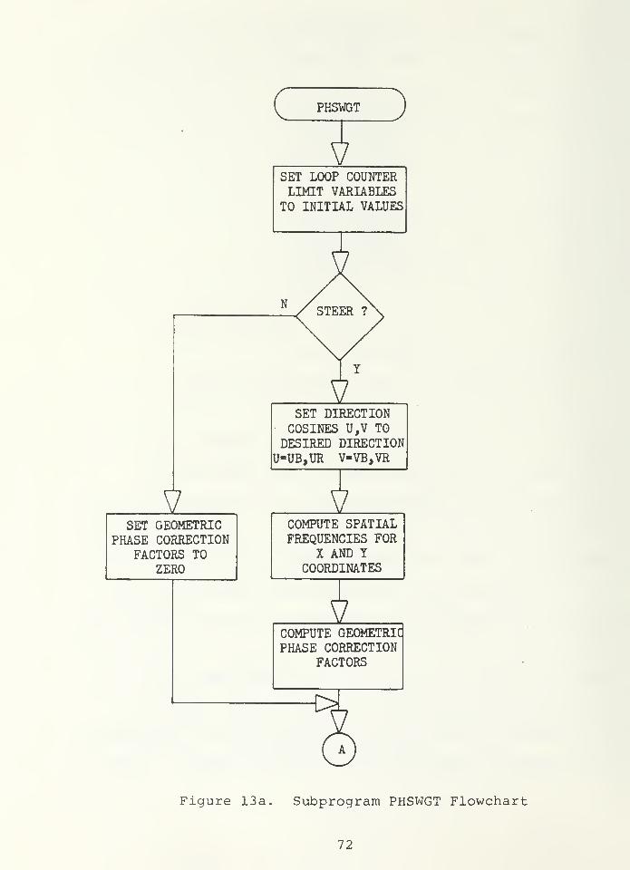
PHSWGT

SET LOOP COUNTERLIMIT VARIABLES

TO INITIAL VALUES

SET DIRECTIONCOSINES U,V TO

DESIRED DIRECTIONU-UB,UR V-VB,VR

ISET GEOMETRIC

PHASE CORRECTIONFACTORS TO

ZERO

COMPUTE SPATIALFREQUENCIES FOR

X AND YCOORDINATES

COMPUTE GEOMETRICPHASE CORRECTION

FACTORS

Figure 13a. Subprogram PHSWGT Flowchart

72

4SET DETERMINISTICPHASE CORRECTION

FACTOR TOZERO

SET RANDOMPHASE CORRECTION

FACTOR TOZERO

N

COMPUTE PHASECORRECTION FORDETERMINISTICMEDIUM

GENERATE RANDOMMEDIUM PHASE

FACTOR

tt

SUM ALL-COMPONENT

PHASE FACTORS4>

c RETURN 3Figure 13b. Subprogram PHSWGT Flowchart

73

are set equal to -u and -v so that the receive arrayo o J

beam pattern points in the -n direction.

The deterministic medium phase correction factor

is found by using equation (2.32) to compute the phase shift

of the signal due to propagation through an inhomogeneous

medium, and then negating the result. The random medium

effect can also be computed from a closed form expression,

but its use in generating phase correction factors is not

the subject of this study, and will not be discussed. The

total phase correction factor for the y-direction is

obtained by adding the system geometry and deterministic

correction factors.

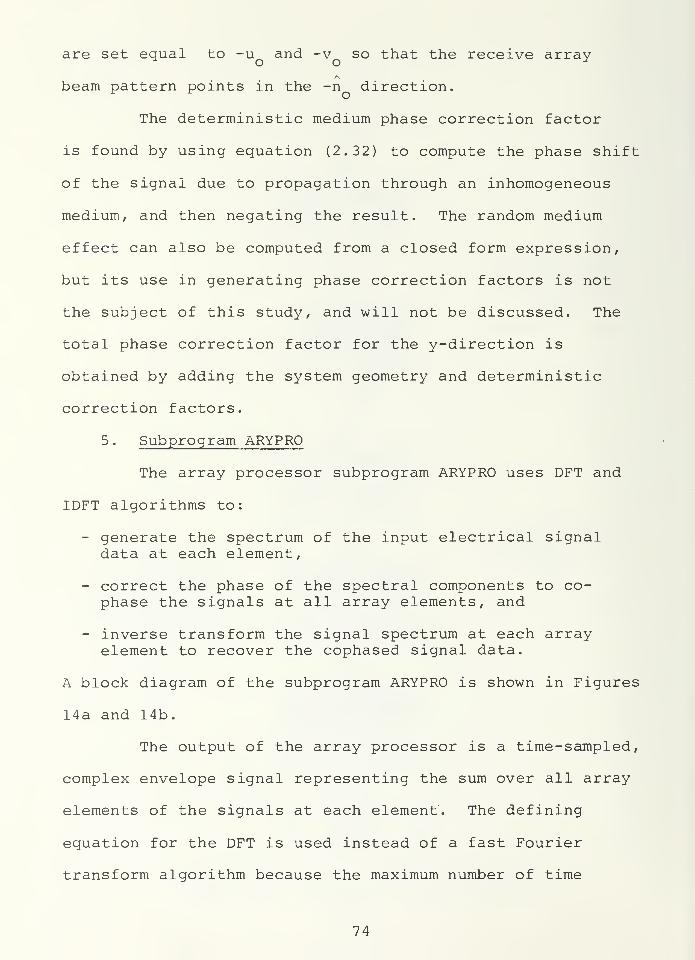
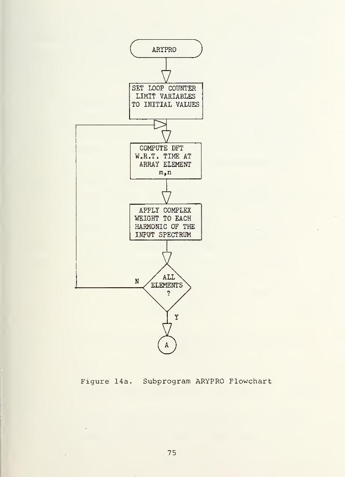
5. Subprogram ARYPRO

The array processor subprogram ARYPRO uses DFT and

IDFT algorithms to:

- generate the spectrum of the input electrical signaldata at each element,

- correct the phase of the spectral components to co-phase the signals at all array elements, and

- inverse transform the signal spectrum at each arrayelement to recover the cophased signal data.

A block diagram of the subprogram ARYPRO is shown in Figures

14a and 14b.

The output of the array processor is a time-sampled,

complex envelope signal representing the sum over all array

elements of the signals at each element. The defining

equation for the DFT is used instead of a fast Fourier

transform algorithm because the maximum number of time

74

ARYPRO

VSET LOOP COUNTERLIMIT VARIABLES

TO INITIAL VALUES

€>5

COMPUTE DFTW.R.T. TIME ATARRAY ELEMENT

m,n

4APPLY COMPLEX

WEIGHT TO EACHHARMONIC OF THEINPUT SPECTRUM

Figure 14a. Subprogram ARYPRO Flowchart

75

COMPUTE IDFTW.R.T. FREQUENCYAT ARRAY ELEMENT

SUM EACH TIMESAMPLE OVER ALL

M BY N

ARRAY ELEMENTS

C RETURN j

Figure 14b. Subprogram ARYPRO Flowchart

76

samples permitted (33) is insufficient to achieve a measurable

improvement in speed of execution [Ref. 6:pp. 151-152].

Additionally, use of the DFT equation relates the structure

of the program directly to previous work by Ziomek [Ref. 2]

and Vos [Ref. 3]

.

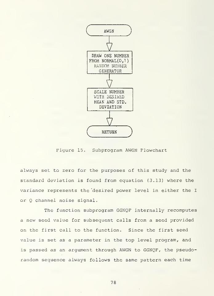
6 . Subprogram AWGN

The function of subprogram AWGN is to generate one

sample of an uncorrelated, Gaussian process with arbitrary

mean and variance. A flowchart of AWGN is shown in Figure 15.

AWGN is based on the International Mathematical

Subroutine Library (IMSL) FORTRAN pseudorandom number

generator routine GGNQF. GGNQF is a function subprogram

that returns one zero mean, unit variance, Gaussian, or

N(0,1), pseudorandom number with each call to the function

subprogram. The zero mean, unit variance pseudorandom

number x is then scaled with the desired mean y and then x

desired standard deviation a using the relation

X = axXn+ px

(3.12

where the standard deviation is computed from the variance

as

a = \/a2

(3.13)x V x

The desired mean and standard deviation are passed

to AWGN as arguments from the main program. The mean is

77

AWGN

DRAW ONE NUMBERFROM NORMAL (0,1)

RANDOM NUMBERGENERATOR

SCALE NUMBERWITH DESIREDMEAN AND STD.

DEVIATION

C RETUHN }

Figure 15. Subprogram AWGN Flowchart

always set to zero for the purposes of this study and the

standard deviation is found from equation (3.13) where the

variance represents the "desired power level in either the I

or Q channel noise signal.

The function subprogram GGNQF internally recomputes

a new seed value for subsequent calls from a seed provided

on the first call to the function. Since the first seed

value is set as a parameter in the top level program, and

is passed as an argument through AWGN to GGNQF, the pseudo-

random sequence always follows the same pattern each time

78

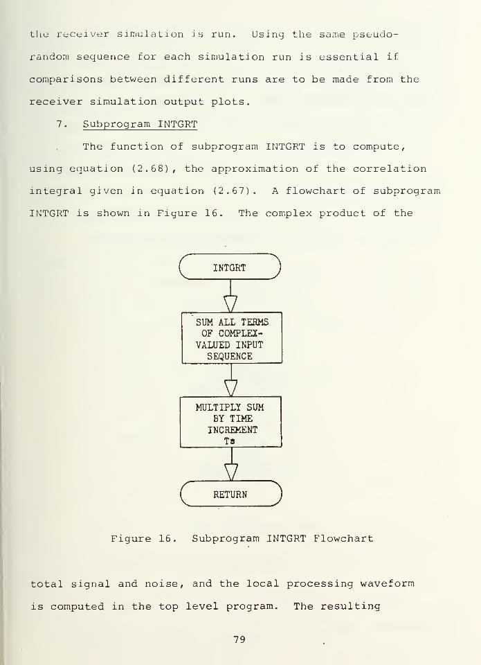
the receiver simulation is run. Using the same pseudo-

random sequence for each simulation run is essential if

comparisons between different runs are to be made from the

receiver simulation output plots.

7. Subprogram INTGRT

The function of subprogram INTGRT is to compute,

using equation (2.68), the approximation of the correlation

integral given in equation (2.67). A flowchart of subprogram

INTGRT is shown in Figure 16. The complex product of the

INTGRT

SUM ALL TERMSOF COMPLEX-

VALUED INPUTSEQUENCE

MULTIPLY SUMBY TIME

INCREMENTTs

RETURN )

Figure 16. Subprogram INTGRT Flowchart

total signal and noise, and the local processing waveform

is computed in the top level program. The resulting

79

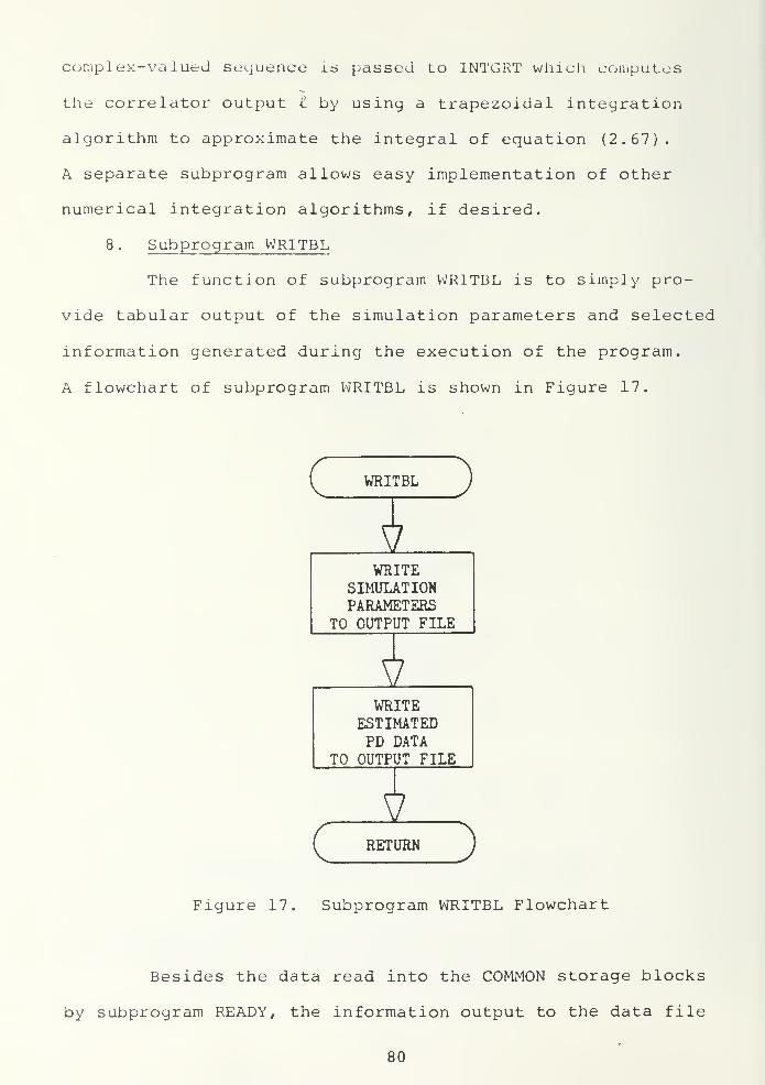
complex-valued sequence is passed to INTGRT which computes

the correlator output I by using a trapezoidal integration

algorithm to approximate the integral of equation (2.67).

A separate subprogram allows easy implementation of other

numerical integration algorithms, if desired.

8. Subprogram WRITBL

The function of subprogram WRITBL is to simply pro-

vide tabular output of the simulation parameters and selected

information generated during the execution of the program.

A flowchart of subprogram WRITBL is shown in Figure 17.

WRITBL

WRITESIMULATIONPARAMETERS

TO OUTPUT FILE

WRITEESTIMATEDPD DATA

TO OUTPUT FILE

4RETURN )

Figure 17. Subprogram WRITBL Flowchart

Besides the data read into the COMMON storage blocks

by subprogram READY, the information output to the data file

80

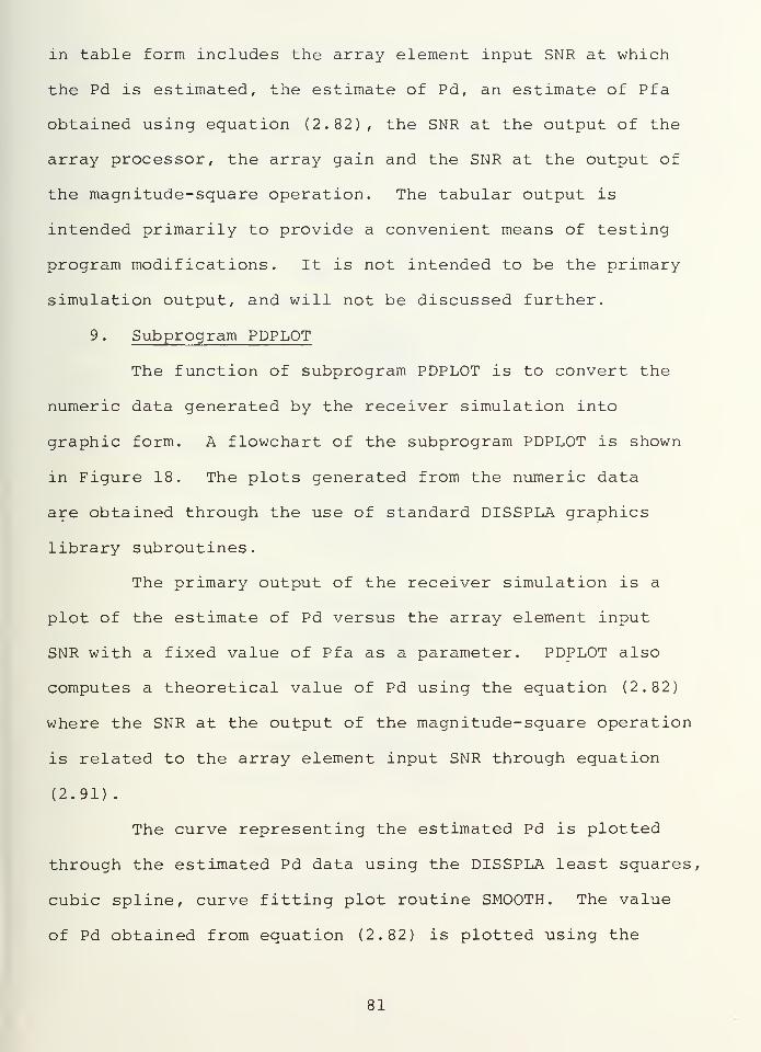
in table form includes the array element input SNR at which

the Pd is estimated, the estimate of Pd, an estimate of Pfa

obtained using equation (2.82), the SNR at the output of the

array processor, the array gain and the SNR at the output of

the magnitude-square operation. The tabular output is

intended primarily to provide a convenient means of testing

program modifications. It is not intended to be the primary

simulation output, and will not be discussed further.

9. Subprogram PDPLOT

The function of subprogram PDPLOT is to convert the

numeric data generated by the receiver simulation into

graphic form. A flowchart of the subprogram PDPLOT is shown

in Figure 18. The plots generated from the numeric data

are obtained through the use of standard DISSPLA graphics

library subroutines.

The primary output of the receiver simulation is a

plot of the estimate of Pd versus the array element input

SNR with a fixed value of Pfa as a parameter. PDPLOT also

computes a theoretical value of Pd using the equation (2.82)

where the SNR at the output of the magnitude-square operation

is related to the array element input SNR through equation

(2.91) .

The curve representing the estimated Pd is plotted

through the estimated Pd data using the DISSPLA least squares,

cubic spline, curve fitting plot routine SMOOTH. The value

of Pd obtained from equation (2.82) is plotted using the

81

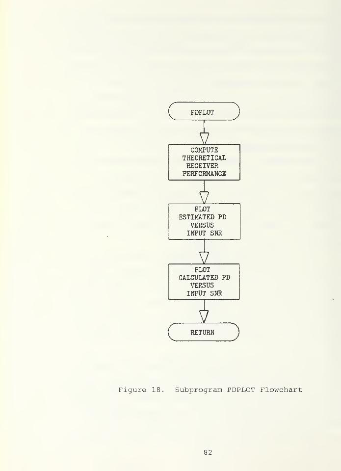
PDPLOT

COMPUTETHEORETICALRECEIVERPERFORMANCE

4PLOT

ESTIMATED PDVERSUSINPUT SNR

4PLOT

CALCULATED PDVERSUSINPUT SNR

C RETURN

Figure 18. Subprogram PDPLOT Flowchart

82

DISSPLA cubic spline, interpolating polynomial routine

SPLINE, and appears as a dashed line on all plots generated

by the receiver simulation. That is, the curve for the

calculated value of Pd is an interpolating polynomial that

passes through the calculated Pd data points, while the

curve for the estimated value of Pd is allowed to pass

within some arbitrary, small offset of the estimated Pd

data point. For the purpose of this study, the maximum

offset allowed was 10 percent of the data point value.

This value of offset provided a reasonable compromise be-

tween obtaining a relatively smooth fit of the plotted curve

without diverging excessively from the data points. Both

the estimated and calculated Pd data points are plotted at

the same array element input SNR.

B. MODEL VERIFICATION

Verification of the receiver model involved two tasks,

characterization of the pseudorandom number generator noise

source, and a comparison of the data generated by the re-

ceiver simulation program with the results predicted by

the theoretical development discussed in Section II. Why

simulate a test case for which a theoretical model exists?

The main reason is to gain some confidence in the results

generated by the simulation when the inputs are such that a

theoretical model does not exist or is mathematically

intractable.

83

1 . Characterization of the Noise Source

The capability to generate noise samples consistent

with the noise description used in developing the receiver

equations is central to verification and usefulness of the

computer simulation. Thus, the first step is to ascertain

the statistical properties of the noise source used in the

computer program. Recall that the assumption required in

developing the relations between Pd, Pfa, decision threshold

and SNR of the magnitude-square of the correlator output

involved the use of zero mean, Gaussian noise which is uncorre-

cted in both spatial and temporal coordinates. The noise

source was tested by taking a sequence of noise samples for

both I and Q channels in manner identical to that used in

the receiver simulation. That is, the subprogram AWGN

was embedded in a test program to ascertain the statistical

properties of the complex envelope of the noise signal. The

following tests were applied to the I and Q channel sample

sequences to verify agreement with the noise process

assumptions

:

- sample mean

- sample variance

- histogram

- autocovariance, and

- estimated power spectral density.

The test algorithms were obtained from standard IMSL

procedures

.

84

Figures 19 and 20 show the results of the sample

mean, variance and histogram calculations for the noise

processes in the I and Q channels, respectively. The sample

mean and variance calculations approximate the zero mean,

unit variance assumptions quite well. The histogram

calculations indicate the distribution of the samples is

roughly Gaussian. The smooth curve plotted through the

histogram represents the exact Gaussian distribution for the

size of the sample window used. The greatest deviation from

Gaussian appears near the mean value which unfortunately is

where most of the sample values lie. Thus, some difficulty

in achieving a perfect correlation between simulated per-

formance and theoretical results was anticipated, and in

fact some deviation from theory at large values of Pd did

occur.

The space-time correlation properties of the sample

sequence was measured by computing the autocovariance func-

tion of 2000 samples over a total time (or space) displace-

ment (lag) of 100 samples. The autocovariance was computed

using the IMSL routine FTAUTO. The correlation of adjacent

samples, whether one or two or 1000 samples apart, was

found to be remarkably small. The autocovariance function

of the I and Q channel noise is shown in Figures 21 and 22,

respectively. Because of the manner in which the samples

are drawn in the simulation, the distinction of a sample

being assigned to a particular channel at a particular

85

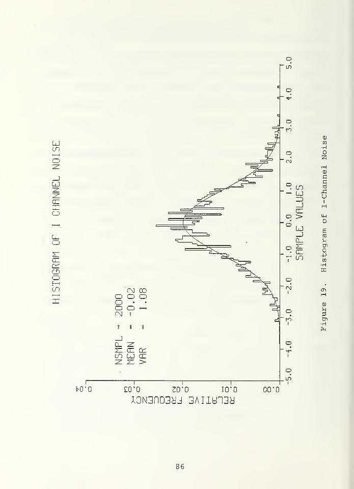
LJCO

LJ

CE

o

L_O

CEcrCDoCO

OoCD

00 cdo CD

CD

wHo

0)

cefO

uI

Hmo

Erd

opw-H

HCU

S-l

Cn•H

q_ -zl

z: ce crCO LJ CE

o•

i

ini

frO'O £0*0 20*0 I0"0

XGN3nD3yj 3AIIU13cd

OO'O

86

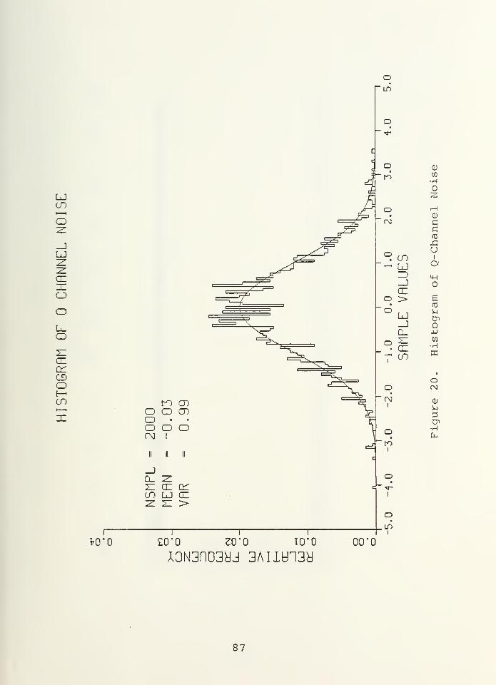
CO

LJZ.ZCEXOoLÔ

ce

CDoCO to CDo o CDo * t

o o oCM 1

II 1 II

_Ja_ zz: ce orCO LJ ce

oLO

o*-

o CD

to w•H

2o H

(Uoo c

c

uo CO 1

.-H LJ a=) IH_lce

o > g• fdo ^1LJ en_J0- +J

o z to

1

CECO

•HK

•

oo CM

i

cu

M

o•

-HPn

roi

C" ^H

ini

WO £0'0 SO'O 10*0

A3N3r)03^J 3AUU13y00*0

87

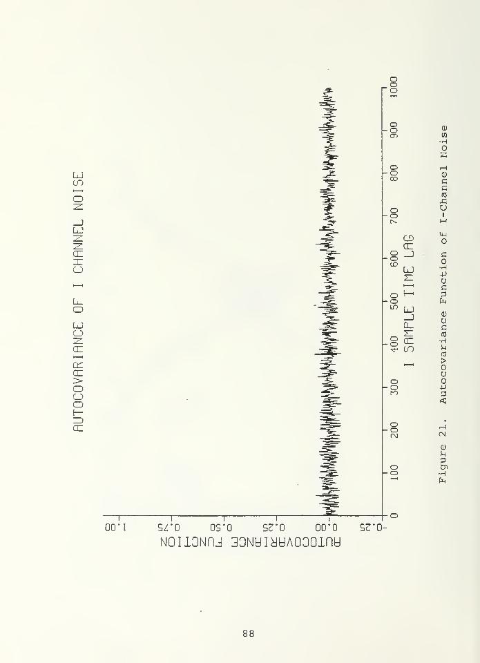
LJCO

O

LJ

en

o

L_oLJO

enen>oCJ>ofr-1

ooo

ooCD

Oooo

oo

ooCD

CDen

LJ

o ^•ow> LJ

_J

.8 5rr CO

oo

oooo

oo

CD

w•H

CD

cc

uI

Hmo

co•H-P

cpEli

ucfO

•H

>ou

-p

CD

u

CnHEm

00*1 SZ'O OS'O S2*0 00"0

NOUGNnj 30NUIdUA000inuSZ'O-

88

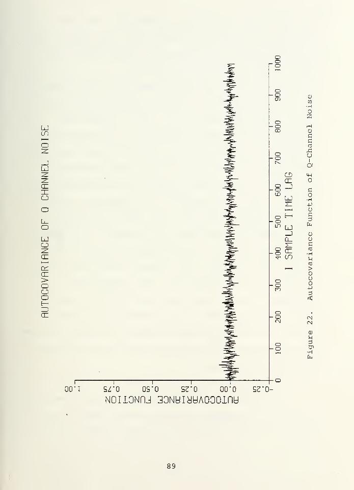
LJen

LJ

coxoo

o

o

CO>ooo

cr

ooo

ooen

ooCO

oo

ooCD

CDcu

LJ

o ô""> LJ

o• o

oo

oo

oo

CCCO

CD

CO

•Ho2

CD

GC

£U

I

aM-l

c:

o•H-Puc

fa

a)

ucfd

H(d

>ooo•4-)

CNCM

CD

U

CT>

•Hfa

OO'I SZ'O OS'O ScTO OO'O

NOIIONDJ 33NUIcdUA000inuScTO-

89

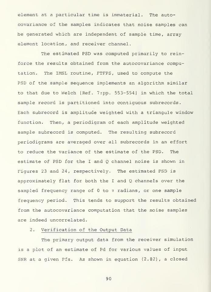
element at a particular time is immaterial. The auto-

covariance of the samples indicates that noise samples can

be generated which are independent of sample time, array

element location, and receiver channel.

The estimated PSD was computed primarily to rein-

force the results obtained from the autocovariance compu-

tation. The IMSL routine, FTFPS , used to compute the

PSD of the sample sequence implements an algorithm similar

to that due to Welch [Ref. 7:pp. 553-554] in which the total

sample record is partitioned into contiguous subrecords

.

Each subrecord is amplitude weighted with a triangule window

function. Then, a periodigram of each amplitude weighted

sample subrecord is computed. The resulting subrecord

periodigrams are averaged over all subrecords in an effort

to reduce the variance of the estimate of the PSD. The

estimate of PSD for the I and Q channel noise is shown in

Figures 23 and 24, respectively. The estimated PSD is

approximately flat for both the I and Q channels over the

sampled frequency range of to tt radians, or one sample

frequency period. This tends to support the results obtained

from the autocovariance computation that the noise samples

are indeed uncorrelated.

2 . Verification of the Output Data

The primary output data from the receiver simulation

is a plot of an estimate of Pd for various values of input

SNR at a given Pfa. As shown in equation (2.82) , a closed

90

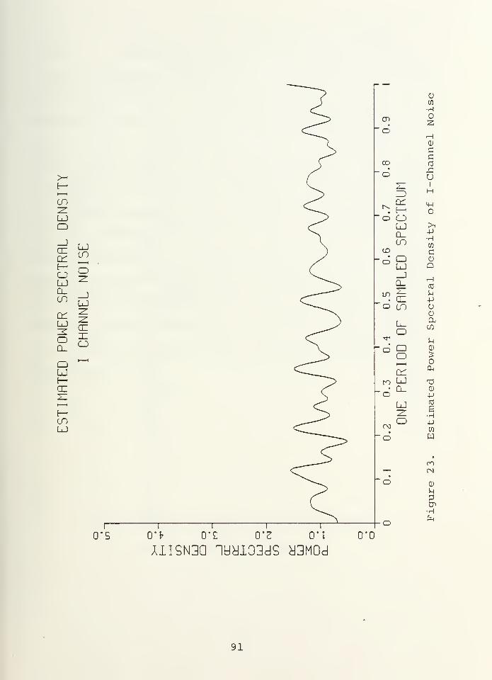
E-*

COZLLJQ

en

U-J

CO

oLJ

o2:

CO _jLJ

LJ

OenJZCJ

Q t—

(

LJt-i

GC2Zi—

i

e-H

COLJ

Q)

CO

•H

CD 2O H

0)

cc

CO 03

o2Z

u1

Z) H

rvC£ mE-"

o OLJ >i

Q_CO

+J

-HCO

CD CQ Q d)

LJ Q_JQ_ H

IT)2Z MCL~ -PO cn O

L_o CO

T uO Q 0)O £

en(X

to LJ TJ• Q_ Q)o -P

LJ 03

g-H

CD +JOJ

CO

o

•

^ cn

oHP

•H&4

0"S O'fr O'C 0*2 0*1

AIISN3Q 1UcJI03dS cJ3M0d

0*0

91

>-i

—Ico

LJQ

enen

oLJ

Ll—l

CO1—

<

o2CO LJ

C£LJ

OQ_

2z:ccn

Q oLJE'-

erz:i——

i

E-h

COLJ

CD

CO

•HCD

o 2H0)

Boo C

03d £TL U

l

ZD O^ oz^ E- IH

o OLJ iNQ_CO •H

CD CO

°S BCD

Q_JQ_ rH

"?£to

5-i

O CO 4-1

CD

L_ OaO COvo S U

CDo SH—

H

C£ fa

to LJ

d^ T3CD

-PLJ t0

:z:' eo •HCO 4-1

•COO w

•

CM

oCD

U3enH

o fa

0"9 O'fr 0"£ 0*2 O'l

XIISN3Q 1UdI33dS d3M0do-o

92

form relation exists between the Pd, Pfa and correlator

output SNR. Furthermore, the correlator output SNR can be

related to the array input SNR when the signals at all array

elements are precisely cophased by equation (2.91).

Therefore, a plot of the theoretical performance computed

using equations (2.82) and (2.91) can be superimposed on

the plot of the receiver simulated performance. The curve

representing theoretical performance provides verification

of the simulated performance when input signal parameters

and phase weighting allow precise signal cophasing to

occur. The computed performance curve also provides a

baseline to evaluate simulated performance when the input

noise or receiver operating conditions differ from the

assumptions used in formulating the receiver model. In

all the plots, the theoretical performance is shown as a

dashed curve.

93

IV. PRESENTATION OF RESULTS

This section presents the results of three receiver

simulation case studies and analyzes the simulation output

in each case. The three cases considered are:

- Case TEST, in which the output electrical signal dataat each array element is produced by a test signalgenerator computer program, and is free of communi-cation channel effects such as attenuation, phaseshifts due to wave front refraction, time delay due torange separation, and the transmit array beam pattern.

- Case HMG1, in which the output electrical signal dataat each array element is produced by the oceancommunication channel simulation computer program,and includes the effects of path attenuation, phaseshifts due to system geometry, time delay due to rangeseparation, and the transmit array beam pattern.

- Case INHMG1, in which the output electrical signaldata at each array element is produced by the oceancommunication channel simulation computer program,and includes not only the effects given in case HMG1,but also contains phase shifts due to refraction ofthe wavefront along the propagation path.

The results of these case studies will be analyzed by

providing a brief description of the transmit signal

waveforms used to generate the array element output elec-

trical signal data, by listing the system parameters that

distinguish the test cases, and finally, by interpreting

the plots of Pd versus array element input SNR for each

case study.

A. TRANSMIT WAVEFORMS

The analysis and theoretical development of the receiver

simulation in Section II makes no assumption regarding the

94

functional form of the transmit signal. The receiver

should perform equally well regardless of the type of trans-

mit signal provided that the correlator/matched filter uses

a replica of the transmit signal as the local processing

waveform. To verify this hypothesis, and thereby test the

integrity of the receiver simulation and the validity of the

assumptions used in generating the model, more than one type

of transmit signal was used to test receiver simulation

performance. The use' of multiple transmit signal waveforms

also provides a broader base from which to draw conclusions

regarding the concept of model-based signal processing. For

the purpose of this research, two types of transmit wave-

forms were used in producing the Pd versus array element

input SNR plots in each of the three case studies.

A rectangular envelope CW pulse and a rectangular

envelope LFM pulse were selected as transmit signals. These

two particular forms were chosen for several reasons. First,

the CW pulse and LFM pulse waveforms were considered to be

typical transmit signals used in SONAR and acoustic signal-

ing systems. Second, the CW pulse provides a simple case

of amplitude modulation while the LFM pulse provides an

example of an amplitude and angle modulated waveform with

considerably different spectral characteristics. Finally,

either signal can be readily synthesized from a finite,

complex, Fourier series whose coefficients c may be calculated

95

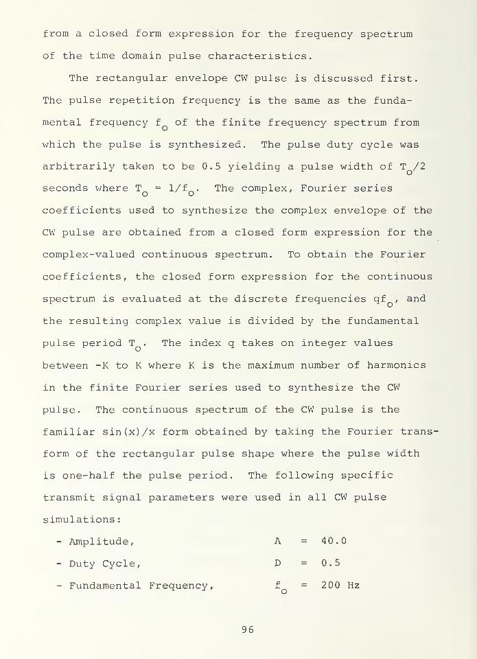
from a closed form expression for the frequency spectrum

of the time domain pulse characteristics.

The rectangular envelope CW pulse is discussed first.

The pulse repetition frequency is the same as the funda-

mental frequency f of the finite frequency spectrum from

which the pulse is synthesized. The pulse duty cycle was

arbitrarily taken to be 0.5 yielding a pulse width of T /2

seconds where T = 1/f . The complex, Fourier series

coefficients used to synthesize the complex envelope of the

CW pulse are obtained from a closed form expression for the

complex-valued continuous spectrum. To obtain the Fourier

coefficients, the closed form expression for the continuous

spectrum is evaluated at the discrete frequencies qf , and

the resulting complex value is divided by the fundamental

pulse period T . The index q takes on integer values

between -K to K where K is the maximum number of harmonics

in the finite Fourier series used to synthesize the CW

pulse. The continuous spectrum of the CW pulse is the

familiar sin(x)/x form obtained by taking the Fourier trans-

form of the rectangular pulse shape where the pulse width

is one-half the pulse period. The following specific

transmit signal parameters were used in all CW pulse

simulations

:

- Amplitude, A = 40.0

- Duty Cycle, D = 0.5

- Fundamental Frequency, f = 200 Hz

96

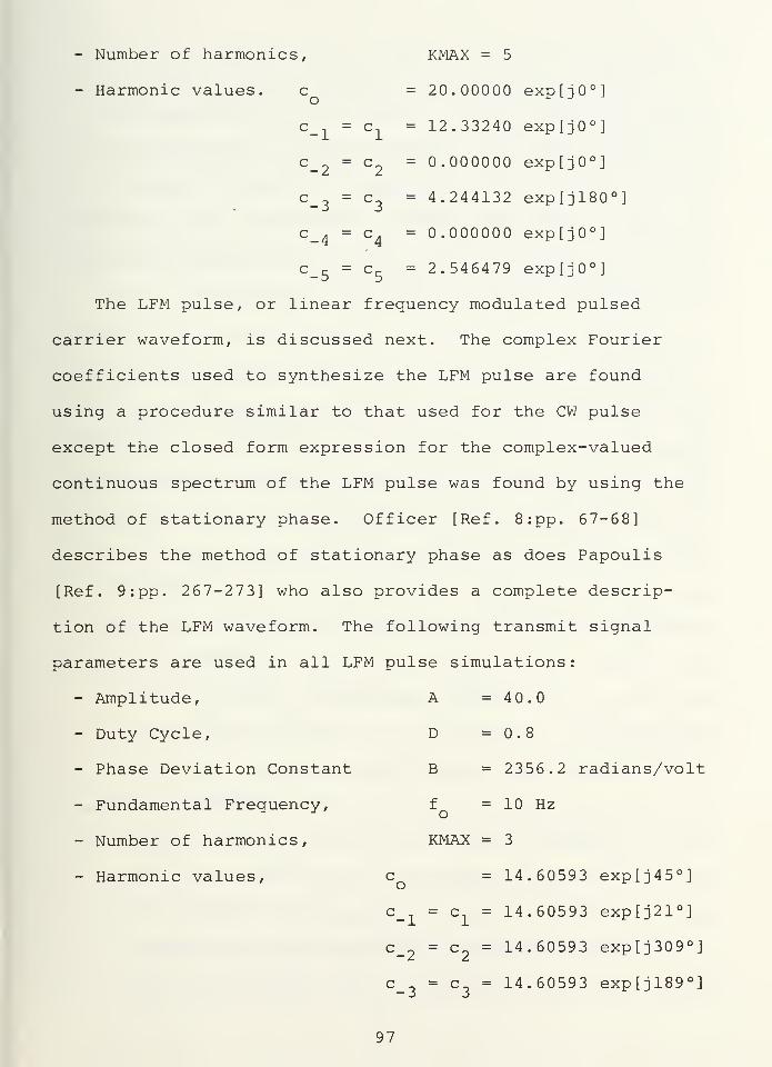
- Number of harmonics, KMAX = 5

- Harmonic values. c = 20.00000 exp[j0°]

c_1

= c = 12.33240 exp[j0°]

c_„ = c„ = 0.000000 exp[jO°J

c_3

= c3

= 4.244132 exp[jl80°]

c_4

= c. = 0.000000 exp[j0°]

c_5

= c5

= 2.546479 exp[j0°]

The LFM pulse, or linear frequency modulated pulsed

carrier waveform, is discussed next. The complex Fourier

coefficients used to synthesize the LFM pulse are found

using a procedure similar to that used for the CW pulse

except the closed form expression for the complex-valued

continuous spectrum of the LFM pulse was found by using the

method of stationary phase. Officer [Ref. 8:pp. 67-68]

describes the method of stationary phase as does Papoulis

[Ref. 9:pp. 267-273] who also provides a complete descrip-

tion of the LFM waveform. The following transmit signal

parameters are used in all LFM pulse simulations:

- Amplitude, A = 40.0

- Duty Cycle, D =0.8

- Phase Deviation Constant B = 2356.2 radians/volt

- Fundamental Frequency, f = 10 Hz

- Number of harmonics, KMAX = 3

- Harmonic values, c = 14.60593 exp[j45°]

c = c = 14.60593 explj21°]

c_2

= c2

= 14.60593 exp[j309°]

c = c = 14.60593 exp[jl89°]

97

It should be emphasized that these complex, Fourier

series coefficients which are used in the ocean communica-

tion channel simulation computer program to synthesize the

complex envelope CW and LFM pulse transmit waveforms are

also used in subprogram SGNLGN to produce the local processing

waveform for the correlator/matched filter detector section

of the receiver simulation computer program RCVR.

B. CASE TEST

The input signal data for case TEST is obtained from a

separate computer program written to synthesize array

element output electrical test signals from a finite Fourier

series expansion of the test signal waveform. The technique

is similar to that used in generating the receiver simula-

tion local processing waveform in subprogram SGNLGN. How-

ever, appropriate phase shifts are added to the Fourier

coefficients to vary the direction of arrival of the plane

wave incident on the receive array, and to incorporate the

time delays due to spatial separation, d and d , of the

array elements. Furthermore, the time delay due to range

and the doppler shift of the test signals are both set to

zero to prevent signal loss in the correlator/matched filter

due to a mismatch between the total array output signal and

the local processing waveform. In this way, array element

output electrical signals are obtained that exclude effects

due to propagation of the sound wave through the ocean

medium, or spatial modulation of the signals due to the

98

transmit array beam pattern. Since the medium effects are

excluded from the case TEST array element signals, the

carrier frequency f is set to zero, and the array element

spacing is increased to keep the interelement spacing d

and d equal to one-half the shortest wavelength in the

transmit signal. Note that this produces different inter-

element spacings for the CW and LFM pulse situations.

Signals generated in this fashion allow the receiver

output to be analyzed separately from the communication

channel. Essentially, it is equivalent to having a signal

generator that provides a test signal to measure receiver

performance. The results obtained from case TEST, when

combined with the plot of theoretically predicted performance,

provides a baseline with which to analyze the receiver

output when the ocean communication channel simulation data

is processed.

The system parameters defining case TEST are as follows:

- Array Parameters

Number of array elements, M = N =5

Array Element Spacing, CW d = d = 0.7375 meters

LFM d = d =24.58 metersx y

- Medium Parameters

Speed of Sound, c = 1475 meters/second

Actual time delay t = 0.0 seconds

Actual doppler shift cf>A = 0.0 Hertz

Four plots representing receiver performance were

generated for case TEST. Phase weighting is done to

99

compensate for the direction of arrival of an acoustic plane

wave incident upon the array elements. The direction of

arrival can be set to any arbitrary direction by the test

signal generator computer program. However, the direction

was chosen to be the same as that due to the system geometry

used in the case studies HMG1 and INHMG1 . Phase weighting

for geometry is indicated by the state of the logical

variable STEER. The estimates of time delay due to range

and doppler shift were both set to zero in subprogram SGNLGN

to maximize the output of the correlator/matched filter

detector. Two of the plots, Figures 25 and 26, show receiver

performance for a rectangular envelope CW pulse. Figure 25

was produced using a Pfa of 0.1, and Figure 26 shows the

effect of a Pfa of 0.01. The remaining two plots generated

for case TEST, Figures 2 7 and 28, show receiver performance

for a rectangular envelope LFM pulse at a Pfa of 0.1 and

0.01, respectively. Since the input electrical signal data

does not incorporate channel effects, phase weighting for

deterministic and random medium effects was not done for

case TEST.

Several observations regarding model performance can

be made by analyzing the plots. Generally for all plots, the

measured performance of the simulation (solid curve) follows

the predicted theoretical performance (dashed curve) , but

the agreement is not exact. That is, the estimate of Pd

follows the same trend as the predicted Pd, but the

100

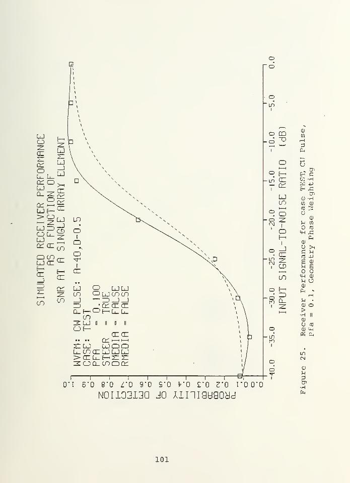
EORMRNCE

E

E— 1

ZLLJz:LJ_JLJ

\

I \

\ \

\ \

\ \

\ \

\ \\ V\ N

ER

PER

TION

cnorct:

cn

D \ N

> CJ•—

• ZLLJ ZDCJ L_LJCZL CE

LJ_jCDZLt——

<

CO

i_n

oiiQ

o colj cn CE

Oii

CE_J

cz

• •

Z3z: ct: LJ O LJ LJ

z^ CO OqjcOcOCD CO

ZD "C£CECEQ.HOHLLCO

Z< LJ II II II II

CJE-<CECE

• • • • fy —( i—

i

ZZLJ LJQQL^COCELJLJLJ> CE L_ t-< XI ZIz< o o_ co o o:

Oo

0"I 6'0 8*0 Z'O 9*0 S"0 K0 £*0 Z'O I'OO'O

N0II03I3Q JO UIIIGUGOyd

ldi

»

o COCD

o ~0 Hi a*

O u•—*

v Cno h^ Eh CLO CE CO -H

1

cnEh A

LJ CD -HCO CO CD

1—

1

<C 5o oo

1

ZL1

0)

u cn

fdO mh s:

l

o _JCZ

£ Sh

f« -PZL e cd

i CD n e—

i

CO <+H CD

Sh cjCDo e—

<

Oi -

o ZD rH

Q_ SH •

1 21—

1

CD O>H II

CD

U (T3o CD MH

LOPi 04

i

•

IDCMo

o CD

rr1

•Hfa

101

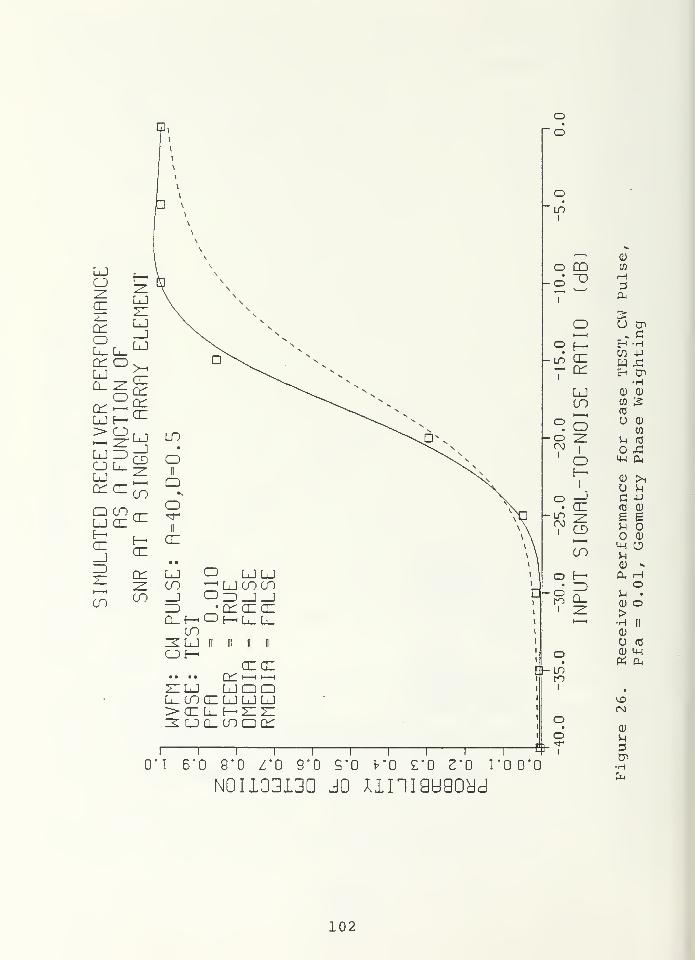
EORMRNCE ELEMENT

\

\\\\\\\s

ER

PER

TION

RRRRY

*"j sn.

RECEIV

R

EGNC

SINGLE

LO•

oIIQ

LJ CE u-O

ii

5 Sii

en

• •

£ i LJ O LJLJCO ^ljcoco

CD ^ _J 03_J_JZD •CCGCCECL_E-< Oh^L^L-

CO2U II II D IIOHCECE

• e • a C£—<--<

21 LJ LJQQL^COCELJLJLJ>CCL_ HZEZ£CJQ_ COOC£

J">-

oo

LOl

o CO

2 2I

o°tlo cncn

i

LJCO

° 5o z:

• cn

CO

h Rc2i 2:

l -LO

oi i^ i i i i i i i i

0*1 6*0 8*0 Z*0 9-0 9*0 fr*0 £'0 3*0 1*0 0*0

Noiio3i3a jo xinigygoyd

CD

CO

<-i

POi

U cn* c

EH -HCO

WE-t

-P

CT>

•HCU CD

CO £(d

cu

wfd

om d-i

S-l

4->

0)

EOCU

M—I OMCU *

ou .

CL) O>•H II

CU

U fO

CU U-i

CU

iT>

•HCm

102

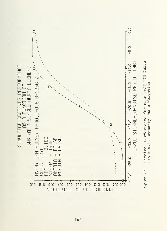
LJCJ

CE

e—<

:z:

LJ

d\V

\

\\

\

11cnoL_ L_cn oLJQ_ 2Ôcn —

<

LJ E—

LJ_)LJ

cm\CDLOfO

ss

CEC£cnCE

CD

CO•

oII

> o•—

1 21LJ ED

LJ_JCD21

CO

CJ L_LJcr cn

IIQo

Q CDcn

E-H

ce

cn

ii

:mulrte

R CE

•

LJCO O LJLJ

ZZL _J Oljcococn CO ED ÊD_J_J

Cn •C^CECEh^ <E)f-^L_L_

ZZCOL_LJ II II n II

_je-«CECE

• • • cn~~XI LJ LJQEDL_ CO CE LJ LJ LJ>cel_ ^ziz:E<OQ_ LOCDCn

D

Oo

1 1 1 B0*1 B'O 9

-

I'O 9'0 9*0 K0 CO 2*0 T'00'0

N0II0313Q JO UHIGUGOyd

loi

r

0)

o QD w

o T) I—

1

p1

c±

O fai i J

oLO

E-h

CEEh CCO -H

l

cn

LJ D~>

CD CD -H

O oCO Q)

O z: CDoo

\u co

1 o tC

E-"

1

CD

o _JCE C S-4

LO 21 tO -Prs]

CD g CD

*~~

'

CO M-l 0)

5-1 Uo E-h <d

• Z3 CU »oto Q_ H

5-1 •

1 21 CU oH—

<

>•H ||

CD

o U rcj

CD 4-1

LO Pi P^to

i

[-•

o CN

o CU

1

u

•rH

fa

103

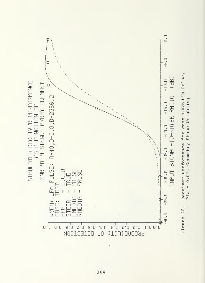
LJCJ

CC

ZLLJz:

D\ \N

N,

(SZoL_ L_

LJ_JLJ

00s

CDLOCO

ER

PER

TION

>-<

CCenenCC

CMII

CD

CO•

II

> oLJ CD

LJ-JCD-ZL

CJ L_LJ

II

CD

CC CC CO OQ CO

CC

E-<

CC

CT

11

LJ CCH<CC_JCDz:

11

CC

•

LJCO O LJLJ

2: _] -—

'

LJCOCOCO CO ID O CD_J_J

Q_ • C£CC CCE-< O HLuLu

ZICOL_LJ II 11 y 11

_Jt^CECE

• • • • cn~~ZILJ LJCDCDL_COCCLJLJLJ>OIL-HCCC£OQ_ COCDCC

oo

o

Lh

N0I1G3I3Q JO Aini9U90yd

in1

Q)

CO"U

H

1

sEn

t—

t

E^ EH -HLO CC 03 -P

1

en

LJ •H

CO cn 5> 1- 1 fOO O O CD

O 2 Wro

1>-i td

1

1O .c

E—1 CU >i

IT)

_JCC2

c +>fO Q)

e e1 CD fi

1—

1

CD

CO M-l CJ

O E-hCD *

Ph hO CD

Cu1 2! CU O

>•H II

U (0

CD 4-1

w>

l

« CM

a

CO

O CN

CD

1

UP

-HEn

104

transition from a low Pd to a Pd of 1 is more sensitive to

changes in the array element input SNR. A comparison

between the plots shows the Pd to be a function of the Pfa

as predicted by equation (2.82), and for small values of

SNR, the estimated Pd approaches the Pfa parameter used by

the simulation in generating the plots. This effect is

also predicted by equation (2.82) since at SNR values much

less than one, the input signal is essentially off, and only

the noise is producing signal detections. A comparison

between the plots for the CW pulse and LFM pulse does show

some minor difference in receiver performance, but the same

general trends seem to hold regardless of the functional

form of the transmit signal.

The differences in the measured performance between the

CW pulse and the LFM pulse simulations can be attributed in

part to the difference in the maximum number of harmonics

used to synthesize the transmit signals. As shown by

equation (2.22), the number of time samples L is related to

the maximum number of harmonics K used to synthesize the

transmit signal. The difference in the number of time

samples causes different subsequences of noise samples to be

drawn from the noise generator subprogram AWGN. The

different noise sample subsequences will cause small varia-

tions in the relative frequency estimate of Pd. Thus, an

exact comparison of the noise performance cannot be made

across different types of transmit signals when the number

105

of harmonics used to create the transmit signal are not the

same. However, the real significance of this effect is that

even with different noise sample subsequences in the I and

Q receiver channels at the array elements, the measured

performance conforms closely to the performance predicted by

theory under the very ideal assumptions of precise signal

cophasing, and zero-mean, white, Gaussian input noise.

For these reasons, it can be inferred that the basic

receiver model is valid, but some difficulty may exist in

generating precisely white, zero-mean, Gaussian noise within

the simulation program. Indeed as indicated in Section

III.B.l, the noise source used in the receiver simulation

does not generate precisely zero-mean, white, Gaussian

noise. Furthermore, the measured Pd is a relative frequency

estimate of the actual receiver performance, and may also

contribute some error in the simulation results.

Considering these approximations to the assumptions used

in the receiver model development of Section II, exact

agreement should not be expected even in the case where the

communication channel effects are excluded. However if

only relative changes or effects are to be observed, moderate

disagreement between the theory and simulated receiver

performance can be negated by comparing only differences in

the estimate of Pd for each of the case studies. A com-

parison of the differences in the measured receiver perfor-

mance will indicate if, and to what degree, the effects due

106

to the physics of acoustic wave propagation can be compen-

sated for by model-based signal processing. The results of

case TEST then can be viewed as a validation of the receiver

model and the applied programming used to implement the

model.

C. CASE HMG1

The input signal data for case HMG1 and case INHMG1 is

produced by the ocean communication channel simulation

program due to Vos and Ziomek [Ref. 3]. For case HMG1 , the

ocean is considered to be a homogeneous medium with respect

to the speed of sound propagation through the water. That

is, the speed of sound is identical at the transmit and

receive arrays, and at all points in between. In this model

of the ocean medium, refraction or ray bending of the sound

wave does not occur. Thus, only phase weighting for geometry

is required, and only those results will be presented. The

homogeneous case provides a needed baseline with which to

judge the effects of model-based signal processing when

inhomogeneous case data is studied.

Since case HMG1 includes the effects of the ocean com-

munication channel, a carrier frequency is used to convey

the modulation through the channel. In case HMG1 and case

INHMG1 the carrier frequency was set to 5.0 kHz. The array

interelement spacing was adjusted accordingly to maintain

the one-half wavelength spacing needed to prevent grating

107

lobes in the array beam patterns. Note that the interelement

spacing was set using the highest frequency expected for

either the CW pulse or the LFM pulse waveforms, and was

kept constant for both the HMG1 and INHMG1 case studies.

The highest frequency occurred for the CW pulse case, and was

equal to 6000 Hz. The estimates of the time delay and

Doppler shift in subprogram SGNLGN were set equal to the

actual values to maximize the correlator output.

The system parameters defining case HMG1 are as follows:

- Array Parameters

Number of array elements, M = N = 5

Array Element Spacing, d = ^ = 0.1229 meters

- Medium Parameters


Actual line of sighttime delay t = 2.033898 seconds

Actual Doppler shift <PA= 0.0 Hertz

- System Geometry (See Figure 1)

Depth of Transmit Array y = 1000.0 meters

Depth of Receive Array y = 2500.0 meters

Cross Range x -x = 500.0 metersr r o

Line of sight range |r-r|

= 3000.0 meters

Eight plots were generated for case HMG1. The first four

plots, Figures 29 through 32, were produced using the

rectangular envelope CW pulse transmit signal. The remain-

ing four plots, Figures 33 through 36 were produced by

the rectangular envelope LFM pulse transmit signal. Figures

108

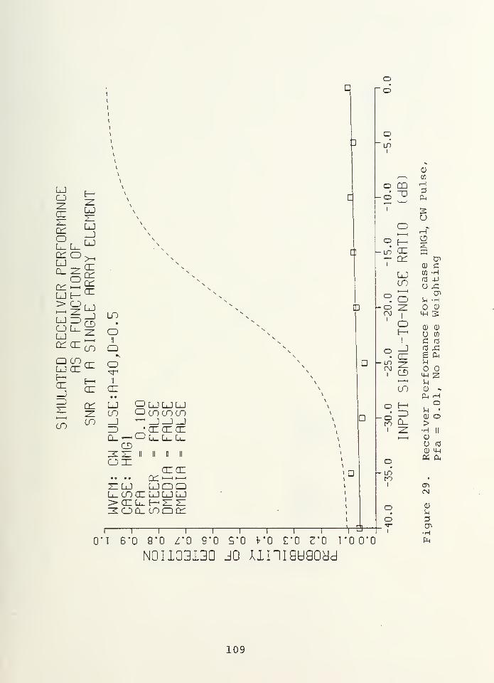
LJOZZce

E—ZZLJZZ

\

\

\

\

\

\

cnoL_ L_

LJ_JLJ

\

\\\

ER

PER

TION

cncncnCE

s

> CDM zLJ ED

LJ_jCDzz

cn

LO

O L_LJcn cn

OIIQ

Q COlj cn cn

*>

OCE E—

CEii

cr

ZD21 cr LJ O LJ LJ LJ

ZZ CO OcocncoCO CO _J rtJJJ

ZD 'CECECECLÔl_LuL.

CDZZ ZZ II II 11 IIor

CECE.... Q^ i 1 ,__,

ZZLJ UDQL-COCELJLJLJ>cel_ t—zzz:E<OQ_LOQCr

ID

[]

D

D

' D

-B

oo

I 1 1 1 1 1 1 1

1

—

t 6*0 8*0 Z*0 9'0 S"0 V'Q £.'0 3*0 1*0 0*0

N0I133130 JO Uini9U90dd

LO1

1—

.

to

O CD Ho ~o

CM

1 2Uo ^rH

o t-H

LO CE B1

cnCD C

LJCO

W -H

£O o U -Ho zz 0)

(M1

m s1 o

<D CDE—

<

1

o _J fa x;

CE e a*

loCM ZZ

CD

5-1

•—

i

S-i

CO (0 -

oo

E-h

ZD

O5-1 •

CD Oro Q_ >

i ZZ •H II

1—i CD

U (0

CD 4-1

o ec; pm

LOro

i

•

CN

o CD

5-1

o 31

CJ>

-Hfa

109

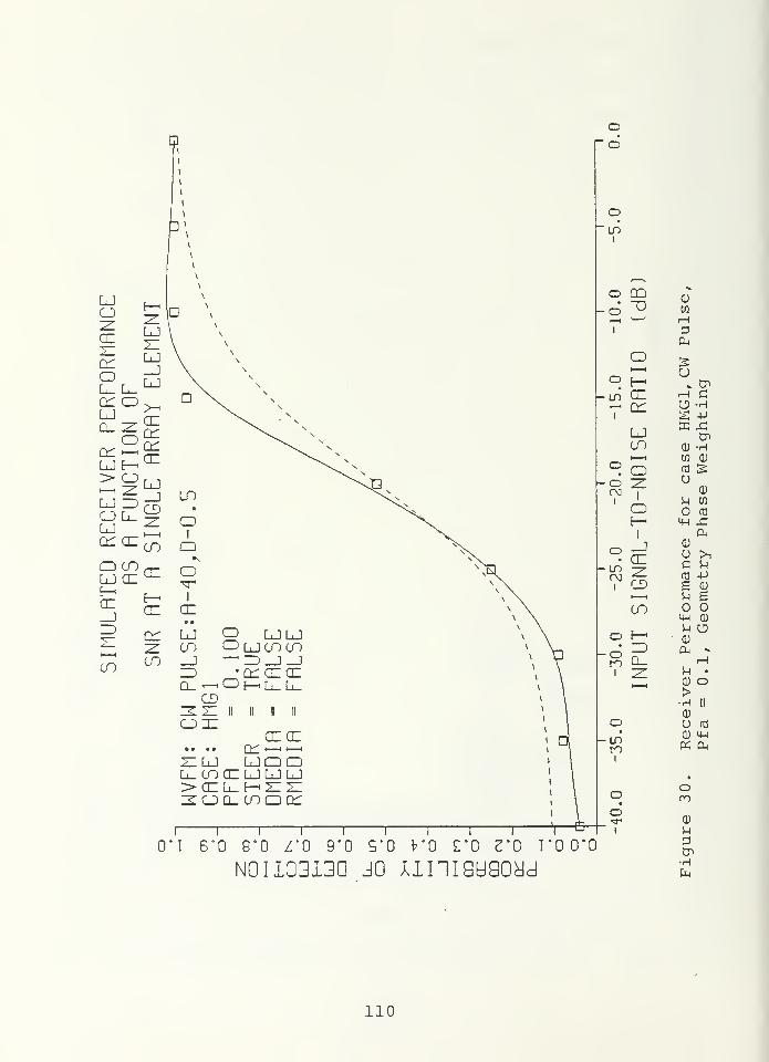
LJ IDCJ Ll_

cn en

q enLJ cc

CE CC

en

o

LJen

Oo

0_ÔCD

2ZUJL_cncc:> cnft_

LjcocnID^_!ft: ccccH^ft_ft_

ccccft:^K-HUDDLJftJLJ

en cd ft:

oo

0*1

—

1

1

f

eo 3*o rocro6"0 8*0 Z'O 9*0 S'O KONoiiG3i3a jo ximauaoad

LO1

O QDCD

O "D

1

HPCM

O £|—"HCJO E-h

.. Cn

m CD rH C

1

ft:

uj CnCO CO -HI—

1

CO CD

03 S2: CJ

1

1

CD

fd

E—

1

I

4-1 SI

mr\3

CD ance

try

1 CD g CD1—-1 U gcn

4-1 CD

b-< CD

ID CU -

ft_ H1 2 Sh •

1—4 CD O>•H II

CD

O ro

1

CD 4-1

« CU

Oco

^r1

1

CD

UaCnHCn

110

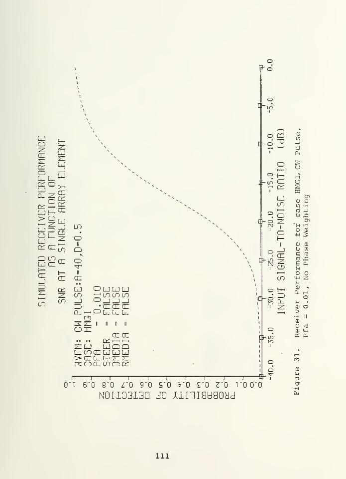
LJCJZcn

LJ2:

\\

\\\\

C£OL_ L_

LJ_JLJ

ER

PER

TION

cuce:

C£cu

> CJ—< z

LJ ZD

LJ_jCDZCO

LO

CJ L_LJ

II

Q COLJ CC cn

CC_l or

II

cn• a

ZD C£ LJ CD LJLJ LJ^— z^ CO —'CO CO CO

cn CO _J O^^^ZD •cccuccCJ—

<

CDl^L_L^CD

3z: 11 11 n 11

ODZCECC

a a a Q^H^H-.XI LJ UDQL CO CC LJ LJ LJ>ccl_ ^zzx:ZOQ-lODtr

oB-6

o

oho

o

1

QQ~0

Cr OCM

[h

OI

_JCUz

v CD

CO

o ("H

iC- o1

I

1 1 1 1 1 1 1 1 1 *T

I 6*0 8*0 I'D 9*0 5*0 fr'O £'0 3*0 1*0 0*0

N0H33I3Q jo uniauaoyd

Cu

O *:hJ "J

M J?

cnC£

LJCO

(U CU) -H

U JS

O CD

0)

UCro

E5-i

OM-l

M

Cm

U •

Q) o>H II

(1)

U fC

<D M-l

ro

0)

T1 M1 p

Cn-HM

111

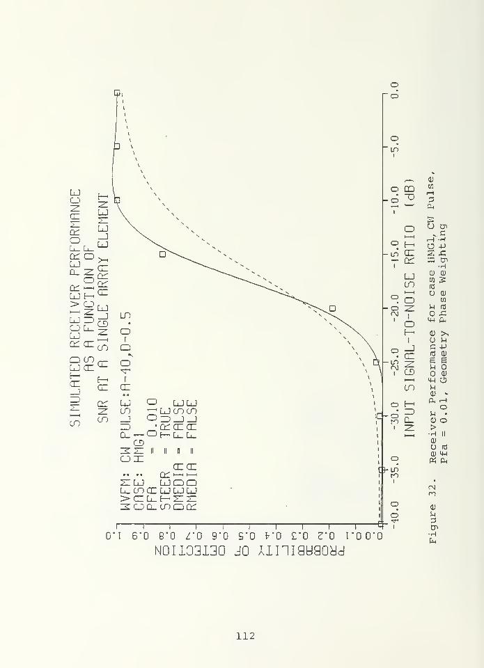
Pi

\

EORMRNCE

E

21LJ21LJ_JLJ

\

\\

X

>

ER

PER

TION

CEcr:

CTCE

lj\^^

> CJ

LJ ED

LJ_JCD

LO

CJ L_LJ

Ocn CE CO

II

CD

ILRTED

R5 CE

E-h

CE

O11

CE• •

z: cr LJ O LJLJH CO —^LJcocnCO CD _J CDlD_J_J

ED •Q1CECEQ_ — CDe-hL_L^

CDe<z: II II II II

ODECECE

• * cn~~21 LJ UDDL_ CO CE LJ LJ LJ>CEL^t— zzz:E<CDQ_ CO CD cn

€

-n

oo

in1

oo

I

om

1

o1

LDro

1

o1

QD

OF—CEcn

LJCO

o

CEZDCD

CO

0_

1 3- LO

1 1 1 1 1 1 1 1 1 r

0*1 6*0 9*0 Z'O 9- 9*0 K0 CO 3*0 1*0 0*0

N0H33I3Q jo unigugoad

o

0)

10

^ ciH -HO -P

2 -Ca Cn

-H0) CD

fd

U CD

CO

fd

.cCm

>1M-PCD

eocu

uoM-l

Q)

Ucfd

s5-1

o

0) -

Cm iHO

M •

QJ O>•H II

CD

U fd

0) <4-l

P5 Cm

CNmCD

Cn•HCm

112

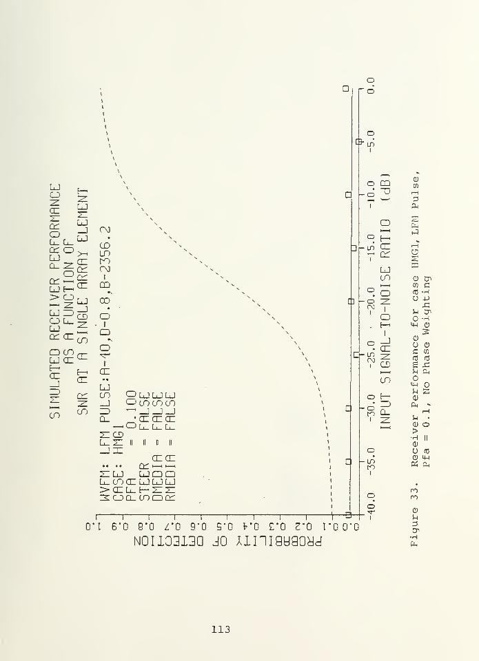
o

LJCJZZ.

CE

E-x

LJZZ

\

\

\\\\

cnoL_ L_

LJ_JLJ

CM

CDLO

s\N

s

ER

PER

TION

>iCECncncn

ii

CD

RECEIV

n

EUNC

LJ_jCDzz.

CO

COD

oIIQ

Q COLJ CE CE

o

cn_jEDzz

CE

cn

CEo •

LJcn CD LJLJ LJ

zz. _j CD CO CD CO

CO CO ED —'-J-J-JQ_ •CECECE—

1

cdl_l_l_EI CDL_EZ II II D II

—}JZCECE

a • • • cn

'

—i—iZILJ UDDL_0OCE LJLJLJ>CEL_ E— XI ZIZUQ_ CO CD 01

CJ-

c

c

o

ol-Ln

CO"D

O

CEcn

LJCO

o

"I1

1 1 1 1 1 1—

&

0*1 6*0 9*0 Z'O 9*0 5*0 V0 2*0 2*0 1*0 0*0

N0H03I3Q jo umaugoyd

h OCM

I

0-in

-oto

I

LOto

I

oo

I

oE-h

CE

CD

CO

E-h

DOQ_

w

Pft

fa

BCD Cnto Crfl -hO +J

x:V-i CnO -HIW 0)

CD

u cu

C CO

fC rrj

£ £U ftO4-) OM 53<D

ft -

Hm •

d) o>

ft ft

nPO

0)

3Cn•Hft

113

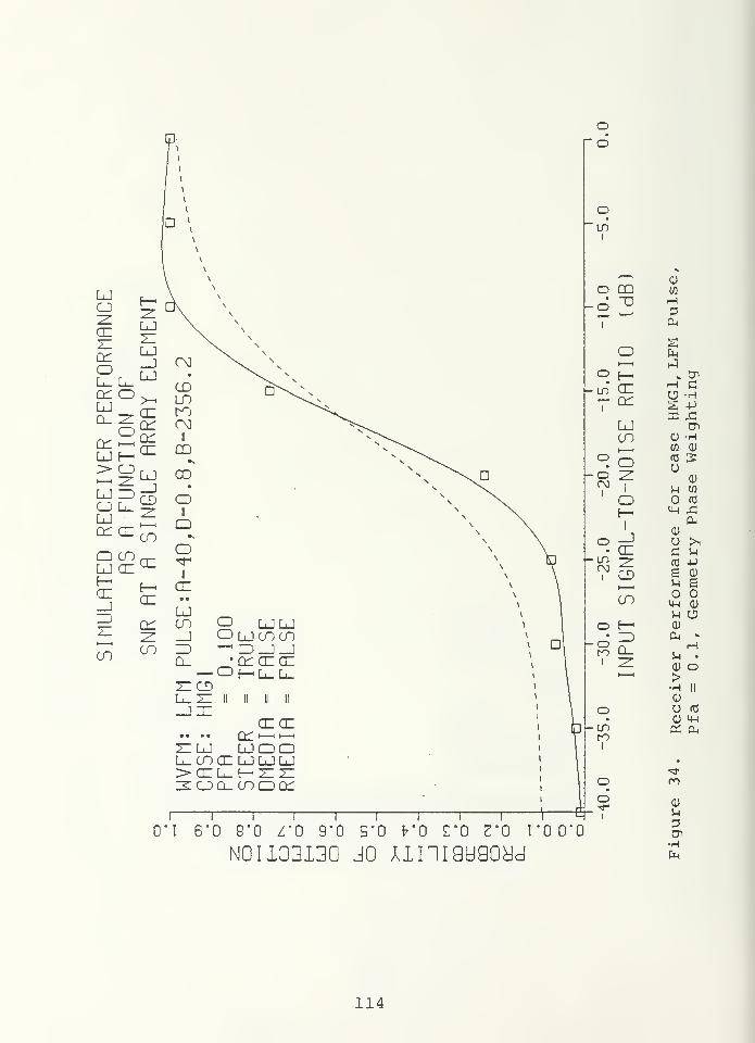
oo

LJCJZZaz

E-i

zzLJ

\

\

\

\

\

^ N

oEoL_ L_cn cdLJQ_ HOcn i—

i

LJ h^

LJ_JLJ

>-<

cm

CDUD

cncncncn

tono

II

CD

> o—< zz

LJ IDCJ L_LJcn cn

LJ_]CD

CO

OII

CD

o cnLJ CC CE

Oii

E—cn_jID21

E-h

CC

cr:

ii

cnm •

LJCO O LJLJ

n _J CD LJ CO CO

CO CO ID ^ZD_]_Ja_ •opener

<—

1

CDh-L_L_ZICDL-ZZ II II II II

_JDZcuce

• • • a cn~~21 LJ LJCDQL_COCE LJLJLJ>CHL_h-2I2IZOL COCDC^

O'l 6*0 8'0 Z*0 9*0 9*0 K0 Z'O Z'O \'0 0*0

N0H33I3Q jo unigugoyd

LD1

, „

CDO CD tn

O1

"D H

O•—

i

Jo f—

'

^ Cn

in

i

cncn HMGl htin

LJ Cn

CO CD -HW 0)o o (0 5u

5-1 Wo

|

zz1o fO

E-|I

1

_!CD

o U >i• CD C 5-1

in ZZ (0 -P

i CD S d)

5-1 £

CO 4-1 CD

5-1 Oo E-« CD

• ID O, -oQ_ H

5-1 •

CD Oi ZZ>H II

CD

o f«

(1) 4-1

u~> « CUro

i

•^*

o ro

oi

CD

5-1

PCnHCn

114

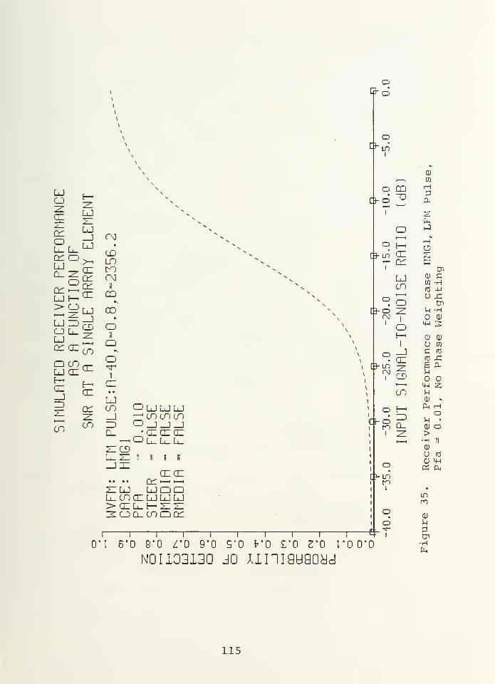
[J-

EORMRNCE

E

e^

LJz:LJ_jLJ •

CDLO

s

ER

PER

TION

>nenC£enCE

COOO

II

CD

> CJ•-H ZLLJ EDCJ L_LJen CE

LJ_]CDZZ

CO

CO

OO

Q COLJ CE CE

11

az_JZDzz

E—CE

en

CE• B

LJCO O LJLJLJ

2: _J '—

'

CO CO CO1—

H

CO CO ZD O^^â_ CECECE

-—

1

O L_L_L_z:cdl_z: II II II IIji

CECE• • • cn^^ZILJ UDQL-COCELJLJLJ>OILHEEzoluidq:

Cr

C3-

1 IB-

1

\

1

t>

oo

oLP

I

[3-

[J-

oLO

I

1

CDT5

CEen

LJCO

o

oE^

I

_JCEZZCD

CO

E—

•

ED0_

I

1 1 1 1 1 1 1 1 1 $"I 6*0 8*0 Z'O 9*0 S'O fr'O £*0 2*0 T'00'0

N0UG3I3Q jo uniauaoyd

o1

CD

CO

H

u

inCD CCO -H(d +J

u x:

in -HO CD

CD CD

U CO

C 03

to xie &oM-l

CD

CD O>H ||

CD

U (Q

CD 4H

nCD

u

Cn•HCm

115

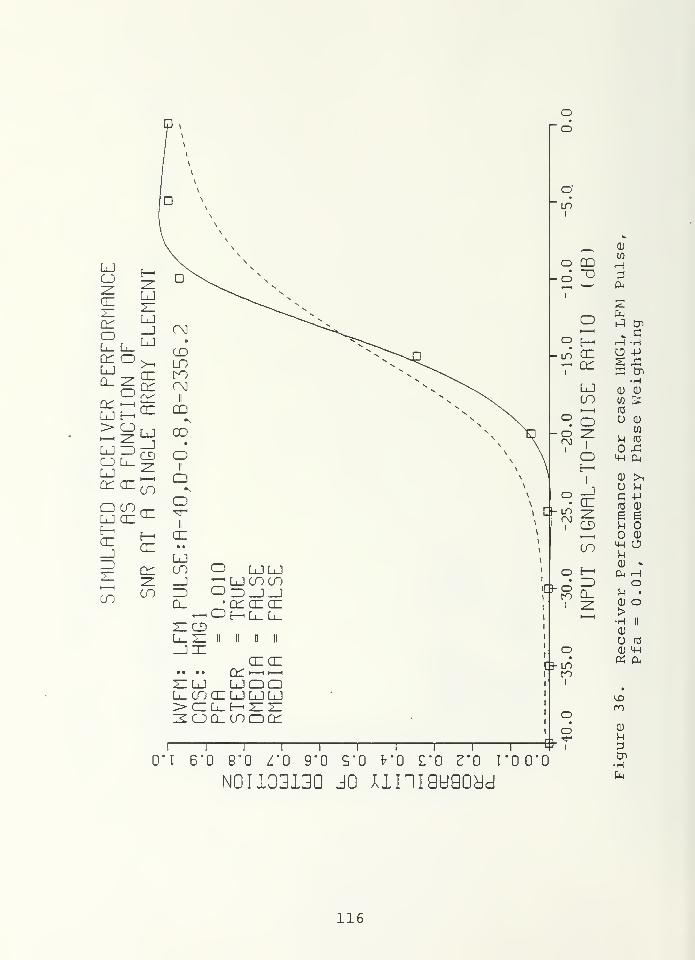
IflNCE

1ENTd\.

XV

"^N. V

cme

CDLO

ER

PER

TION

RRRRY

11

CD

RECEIV

R

EUNC

SINGLE

CO

II

lj az u-11

1ULRT

RRT

GC• e

CO O LJLJtz 2: _J ^L±Jcocnen en ID Oid_]_j

Q_ •CECECE*—

<

Oh^L_L_ZICDl^ZZ 11 11 n 11JI

en a:• • • or^^ZILJ UDQL^CnCCLxJLJLJ> CTI L_ E— ZI ZIZOQ-LODCt:

CD

10

HPCu

SfaJ C7>

iH -HO -P

•HCD CD

w 5rd

u aj

CO

o s:

uc -pfd qj

Eo0)

O'l 6*0 8-

Z*0 9'0 S'O fr'O £*0 2*0 I'OO'O

N0I133I30 30 UIIIGUGOyd

uom ouCD -

OU '

CD O>•H II

CU

u rd

Pi 0^

ro

CD

P&•Hfa

116

29, 31, 33 and 35 show receiver performance when no phase

weighting is done. These plots indicate that performance

will be very poor when the output signals from the array

elements are not cophased. Again, it is significant that

the Pd in this case is approximately equal to the value of

the Pfa parameter used in obtaining the plot. That is,

the total array output signal must be very small because

of destructive interference of the array element signals,

and the only detections appear to be due to the noise.

Figures 30, 32, 34 and 36 show performance when phase

weighting is done to compensate for system geometry. These

plots indicate receiver performance can be made to approxi-

mate the theoretical predicted performance if the individual

array element signals can be cophased to provi.de constructive

interference at the output of the array processor.

Figures 29, 30, 33 and 34 show receiver performance at

a Pfa of 0.1. Figures 31, 32, 35 and 36 show the effect of

decreasing the Pfa to 0.01. The effect of decreasing the

Pfa on the simulated performance follows the theoretically

predicted performance and provides further confirmation that

the computer implementation of the model is accurate.

The important conclusion from case HMG1 is dramatic

improvement in receiver performance is possible provided

that enough information about system geometry exists to

generate phase weights that will properly cophase the array

element output signals.

117

D. CASE INHMG1

The input signal data for case INHMG1 is produced in

the same manner as case HMG1. The transmit signal waveforms,

system geometry, and transmit and receive arrays are identi-

cal. The only difference between the two cases is the

model of the ocean medium. For case INHMG1 , the ocean is

considered to be an inhomogeneous medium with respect to the

speed of sound propagation through the water. The speed of

sound is assumed to vary linearly with depth (or y-coordinate)

only. That is, the speed of sound is not identical at the

transmit and receive arrays. In this space-variant model

of the ocean medium, refraction or ray bending of the sound

wave does occur, and the model of the ocean medium due to

Ziomek [Ref. 2] predicts what the phase shifts in array ele-

ment output electrical signals will be. Using this knowledge

of the physics of acoustic wave propagation, phase weights

are generated that attempt to compensate for the refraction

of the acoustic wave along the ray path, and the system

geometry. To determine the effect of this model-based signal

processing algorithm, the inhomogeneous data was also

processed using phase weights that compensate just for sys-

tem geometry. The difference in simulated receiver perfor-

mance between these two situations will graphically show the

effectiveness of the model-based signal processing approach.

The system parameters defining case INHMG1 are as

follows

:

118

- Array Parameters

Number of array elements, M = N = 5

Array Element Spacinq, d = d 0.1229 meters2 r v x y

- Medium Parameters


Gradient g = .017

Actual line of sighttime delay t, = 2.033898 seconds

Actual Doppler shift cf>A= 0.0 Hertz

- System Geometry (See Figure 1)

Depth of Transmit Array y = 1000.0 meters

Depth of Receiver Array y = 2500.0 meters

Cross Range x -x = 500.0 meters3 r o

Line of sight range |r -r|

= 3000.0 meters

Twelve plots were generated for case INHMG1. The first

six plots, Figures 37 through 42 show receiver performance

for a rectangular envelope CW pulse. The remaining six

plots, Figures 43 through 48, are the result of a rectangu-

lar envelope LFM pulse transmit signal. Differences in

receiver performance due to the form of the transmit signal

are measurable, but not significant.

Figures 37, 40, 43 and 46 were generated when no phase

weighting is applied to the array output electrical signals

Again, these figures indicate that the array element output

electrical signals must be cophased to provide any useful

detection capability in the receiver.

119

LJCJ

ce

z^LJz:

V

\

>

\

cc:oL_ L_

LJ_JLJ

\

\

R

PER

ION

>HCEcncnCE

\

v

LJ E—

RECEIV

EUNC

LJ_JCD

CD

LOD

oIIQ

Q COlj ce CE

•-*

Oe-h

CE_J

E-h

CEII

CE• e

ZDz: C£ LJ CD LJ LJ LJ

Z^ CO C-'cococnen co _J—* ^_j_j_j

EDC£) •CECECCo_z: Ol_l_l_

IEZ<Z II II II II

O—hCECE

• e • • cn —h^ZILJ UDDL_COCELJLJLJ> ce l_ e-< z: z:ZOILCDDQ^

o

B-

LO1

CD' '

*

ino LU Ho "O

CM

om

i

oi

OE-h

CEcn

LJcn

i 1 1 1 1 1 1 1

1

—

I 6"0 8*0 Z'O 9*0 5*0 fr*0 CO 2*0 TO D'O

N0II33I3Q JO Uni9U90y<d

oCO

I

LOro

i

oI

D_

U

SK2

<D tr>

CH-P

O -H

E-h1

o _JQ)

U CD• LL c w

u> 7" d fdi

1CO e .c

i—

i

M Cn

CO m o

o E-h CD- ZD Cn -

5h •

CD O>•H II

CD

U (C

CD 4-1

Oh Cm

ro

CD

U

•HEn

120

D

CJZZ

E—ZZLJZZ

s

\

\

\

\

oL_ L_

LJ_JLJ

\

\

\ss\

R

PER

ION

CZC£orCZ

\s

LJ E—> CJ

LJ ID

LJ_]CJ

LO

CJ L_LJ

II

Q^ OZ CO QQ COLJ CC CU OCC_J az

II

CE

ZD C£ LJ O LJLJzz CO CD lj en CO

1 1

CO CO -J^^ZD—1—iZDCD *cc:czcza_zzcz^L_L_

zzZ£ zz 11 11 n 110—

<

CECZ.. .. ££_<»_ZZLJ UDDL_ CO CU LJ LJ LJ> CZ L_ E-< 2Z 2Zzoliodq:

1 z

oo

LO1

O DJ

CD

[fl

1—

1

O ~D 3Cm

oLO

I

LOOO

I

1 r~°"I 6*0 8*0 Z'O 9*0 S'O fr'O CO 2*0 T'00'0

N0II3313Q jo umauaoad

E-«

CZen

LJCO

o ZZ

E-<

I

r-i -JCZzzCD

CO

o E—

1 ^

LOro

1

o1

U

s cre -h2 -pH £

CnCD -HW CD

fd 2u

CD

5-1 en

o <d

0)

u >i

(d 4-1

e <u

C eo

4-1 0)

5-1 CJCD

Cm -

HM •

CD O>•H II

CD

u fd

CD 4-1

Pi Cm

00

CD

U

121

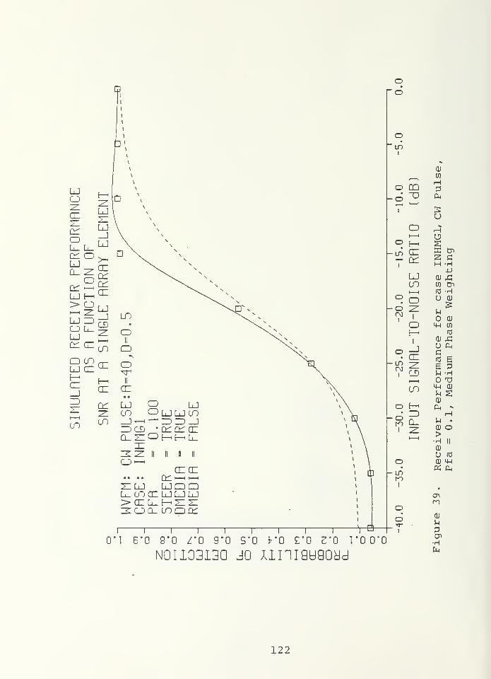
LJCJLJ(H

QLJ

az E'-

enii

en ljoljljcd^—<—<E)E)_J

zdcd -C£C£ cecleOhhlz:

II D II

cece

zilj ljddl_coceljljlj> ce l_ e— x: z:e<oq_ cnocr:

od

11 1 r~ ~~r~ ~r~ ~~r~ ~~

r

0"I 6'0 8*0 Z*0 9*0 S*0 fc'O £'0 Z'O 1*0 0*0

N0HG3I3Q jo mnigugoad

1

CD

WHO CD 3

o ~D &<

1

uO rHi—

i

oo E-| iLD CE K tP

1

C£ H -H

LJ CD £CO 10 tr>

i_, (0 -HO

OCO

oz:

i

U 0)

UCDo MH CO

|

CD £O _J

• CE rd 6inno z: 6 3

i CD 5-1 -HH3

en hh cd

H 2CDo E-h Oh >

• E) rHoCl_ >H •

i z CD O>•H II

CD

o to

o CD MH• Ph CU

u~>

i

•

oo

i

CD

CnH

122

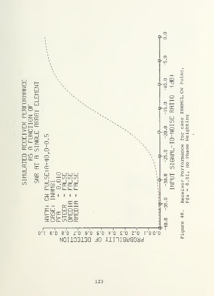
LJCJZZ.

CE

E—

<

zz.

LJ

\

\

\\\\\2Z >v

C£OL_ L_

LJ_JLJ

sN

R

PER

ION

cecôr:

ceLJ E—> O—• z:

LJ ED

LJ_JCDZ<

cn

LO

O L_LJcn az

oiiQ

OCT)LJ CE ce OE-"

ce_j

e-<

cnii

CE•

EDz: C£ LJ oljljlj

zz CO -1 CO CO CO

CD cn _)—

'

o^^_jZDCD •(XCECEo_z: <=>L_L_L_

IEz^zz II II 1 IIo^

cece• • Cn —it—

i

ZZLJ LDDL_COCELJLJLJ:> ce l_ e-< x: x:Z< CJ Q_ CO CD C£

o0-d

o

OQfr- O

oP0- LO

I

CO"O

c-

[J-

CEcn

LJCO

Oor\)

i

i[- oto

i

I 1 1 1 1 1 1 1 1 1

0*1 6*0 8*0 Z'O 9'0 9*0 K0 £*0 2*0 TO O'O

N0I13313Q JO Uni9U90yd

CEZZCD

CO

h^ZD

[ hLOro

oo

CD

CO

i-H

P

U

o

2Cn

CD CCO -HfC 4J

U -CCF

U -H<D

CM 5CD CD

u to

e cu

—i

CD -

OU •

CD O>•H II

CD

U fd

CD M-l

o

CD

5-1

Cn•Hfa

123

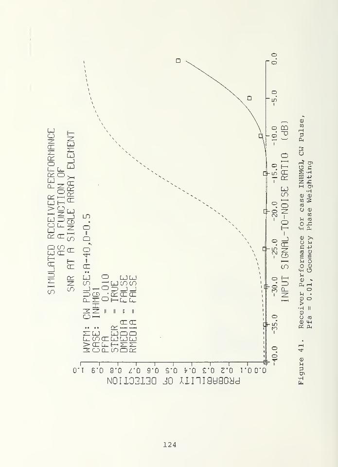
FORMRNCE

F

ZLLJ

LJ_JLJ

\

\

\\\\\

NN

R

PER

ION

>-<

cncncncn

-

LJ E-i

> O•—

i ~ZL

LJ ID

LJ_jCDzl

LO

CJ L_LJ

Ocn cn

i—i

cnII

ILRTED

R5 cn

cn

Oii

cn• e

z: err LJ O LJ LJ^: cn ^LJcncnt—

i

cn CO _jÔDJJZDCD 'cnazazclz:OhLL

JZzzz: II II 11 II

o—<cncn

• • • • cn>—ii

—

'

2ZLJ LJQQLx_ cn cn LJ LJ LJ>cnn_h^z:z:zoi lodq:

o

i[3-

oo

LOI

Oo

I

CO

cncn

LJcn

L>

C-

oto

I

O

O

cnZLCDt—

1

cn

IDQ_

I 1 1 1 1 1 1 1 I 1 wO'l 6'0 8*0 Z*0 9*0 9*0 K0 CO Z'Q I'OO'O

N0U33I3Q jo uniauaoyd

ChLO

o

cu

wH

u

O GS -HIX! -P

H cn•H

CD CD•—

<

W Sto

U Q)

M

O 434-1 Cm

5-1

4-1

CU

go

4-1 O5-1

CD »

Cn -HO

5-1 •

CD O>•H II

CD

u td

CU 4-1

« a.

CD

5-1

CT>

•HEn

124

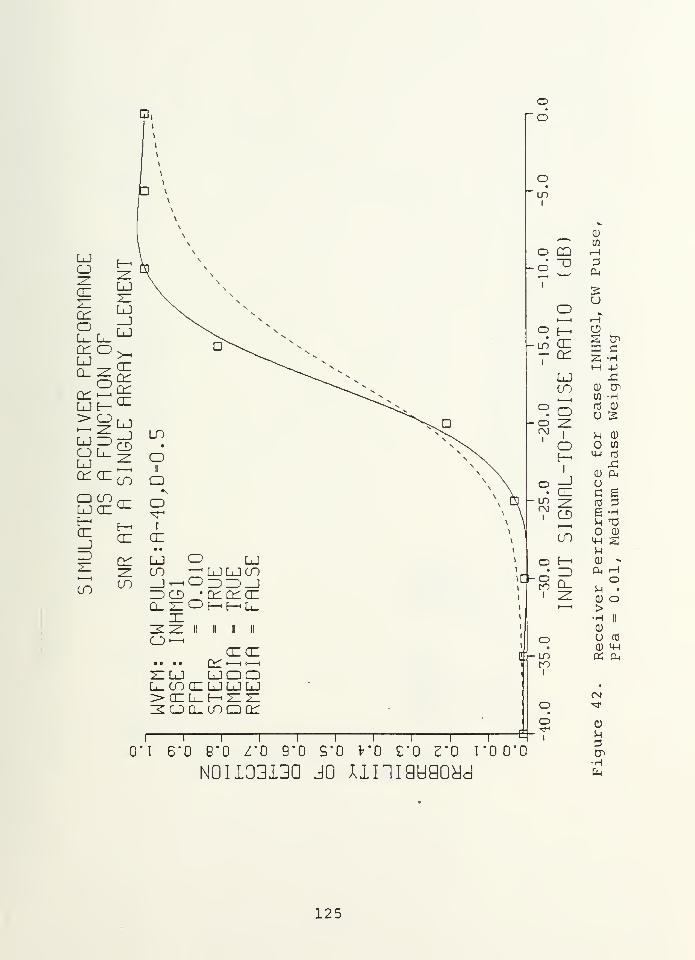
1RNCEMENT

\

\\

\\\

° r i

ER

PER

TION

RRRRY

u\^^

RECEIV

R

EUNC

SINGLE

LO

OIIQ

lj en u-

5 =

Oii

en• •

S i LJ O LJCD -^LJLJCn

en ^ _J—

<

0=)=)_JZDCD •C£C£ enclz: OHHL.

en en

zilj ljqql_ co 01 lj lj ljxxil^h^xzz:

QJ

CO

HPa,

u

oS cpEm C

M -P

CO -Hrd CD

U 5H

<D

OC

e

o4-4

a;

Oh

>•HQ)

UCD

«

QJ

W

E3•H

<D

id

4-1

04

0"! 6*0 8*0 Z'O 9*0 S'O K0 £"0 2*0 I'0 0'O

N0I133130 JO uniguGoyd

CN>*

CD

UPC*•HPn

125

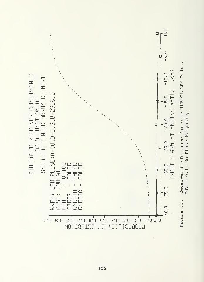
LJCJ~ZL

CE

21LJ21

\

\

s

\\

cnoL_ L_

LJ_JLJ

CDLO

NN\

cn o >iLJQ_ 2ZOcn —

<

LJ E—

>

CEororCU

roOJ

II

CD

> o—< 21

LJ ID

LJ_JCD

COe

oCJ L_LJcn az

21

CO

IIQcd cn

CCO

lj azii

E-h

CE_JID21

cn

cr:

CE

LJCO CD LJLJLJ

21 —

]

CDcococoCO CO ZD—

<

^ _]_]_]CuCD •CECECE

21 d>L_L_L_

L_ ii ii n

CECE.... q^ i—i

,—

,

2ILJ UDDL_ CO CE LJLJLJ>CEL_h- 21 21300.1000^

oPro

o

oh O

I

[]

CI

[]

I I I I I I I I I I

t 6*0 9*0 Z'O 9'0 S'O fr'O £"0 £"0 TON0I103I3Q 30 uniauGoyd

QD~o

o

I

h OCM

I

I

t-oto

I

-LOto

I

oo

I

O'O

in

2Cn

oCE.cn s

HLJCO CU Cn

cn cl-—'

fO -Ho -P21 £

1

j-j cr>

CD -H

E—

•

|S»

1 CU

_J U CU

CE C CO

21CD

re (d

g £M Cu•—

CO M-l

u zE-i CU

ID

CU o>•H II

CU

U ftj

CU M-l

« cu

CU

5-1

POi•Hfa

126

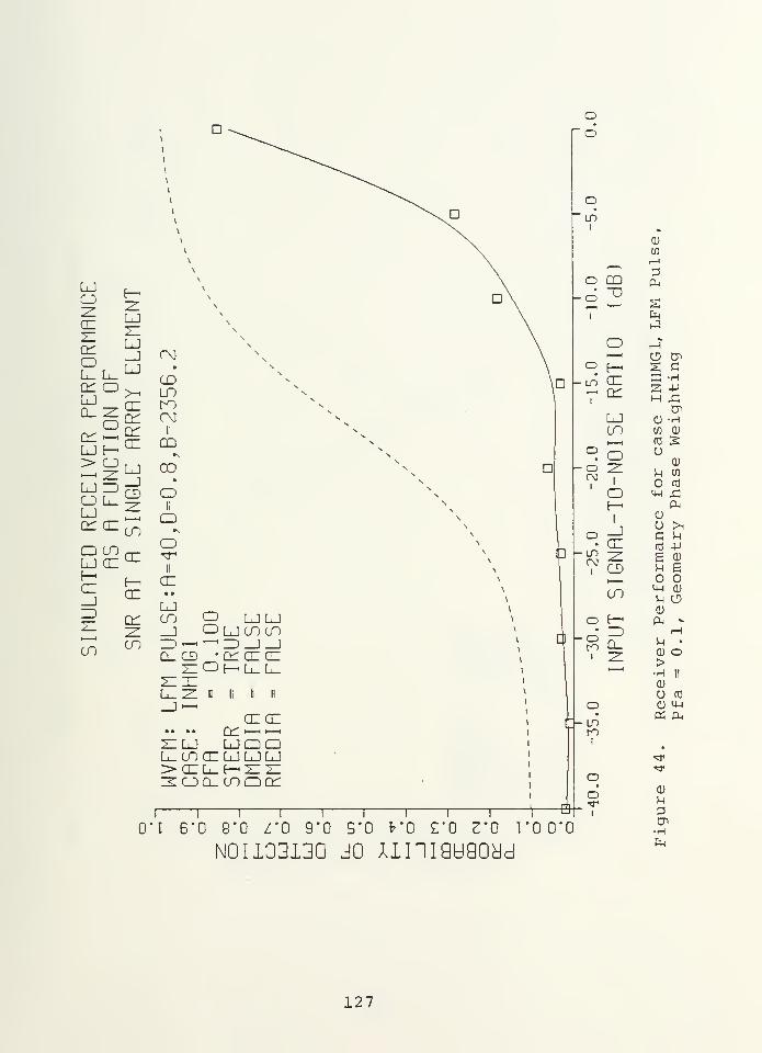
LJCJ E—

~ZL

LJZZLJ_JLJo

L_ L_CT OLJQ_ ^ cr

C£

LJ E— CE

sy^LJ ZDO L_LJ

i

CDZZ

cn ce cn

q cdenlj cn

CE_]

E-h

cr

3z: cn

CD cn

D

fM

CDinCO

ii

CD

CDe

OIIQO

LJCD O LJ LJ

Oljcdco

a. cd 'cncn.cn

z:xL_ "Z. II II II II

_J~ctce

• • •• Q^; —< i—

i

ZILJ UDDL_COCE LJLJLJ>CELHZZzolcodq:

- o

in CL

II-

O'lI

1^

6*0 8*0-B

oo

oin

o CO

i

• ono

i

CH

LJCO

OZZ

IOI

•in ~z-

CD

o E-h

"Rc?

toI

Ocr1

i

Z"0 9"0 9"0 fr'O £'0 2'0 I'00'O

N0UG313Q jo uniauaoyd

cn

i—

i

PCl<

S c

2 -PH X!

0) -HCO Q)

uQJ

u cn

fd

m £SPu

OJ

O >iC Mn3 -P

£ QJ

H £o o4-1 Q)

M O0)

s-l•

0) o>•H II

0)

U (d

Q) Hhft Pn

<3<

•^r

0)

n30^•HCn

127

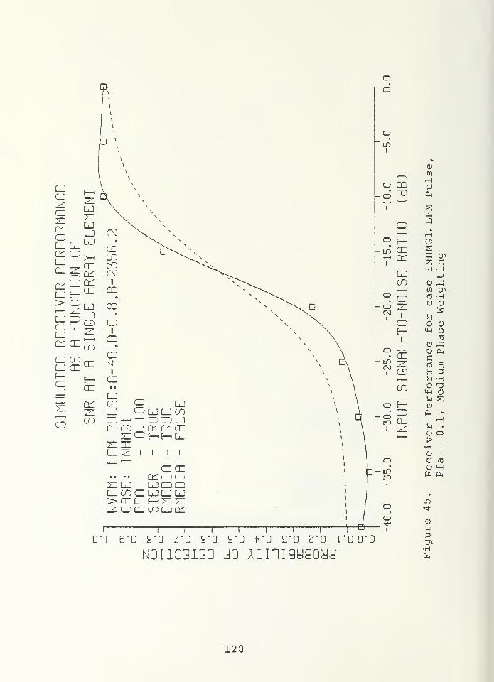
ER

PERFORMANCE

TION

OF

E—ZZLJZZLJ_JLJ

>-i

On]

COLO

\

\

\

\

\\\

*\en

CE

Ox]

II

CO

RECEIV

A

FONC

LJ_jCDZZ

CO

CO

oII

CD

o coLJ GC az

oXT'

ii

CE_JZD

az

ii

aze s

LJCO O LJ

ZZ ZZ _J cd ljljco1 <

CD CO zo — ^ZDZO JQ_CD •czcuaz

z: d F—t E-h L_ZZZZL_ZZ II II II II

_3—azaz

a e • • (V i

—

ii—

i

ZZLJ LJCDCDL_COCZLJLJLJ>gzl_^zzzzzsoQ-coocr:

oo

IDI

O CO

2 2i

oLO

I

oI

E—CZcn

LJCO

oE-h

I

• az

CO

o E-«

LOto

I

oI

0*1 6*0 8*0 Z*0 9'0 9*0 *"0 CO 2*0 1*00*0

N0H0313Q jo Ainiguaoyd

to

iH30^

El,

si en2 cH -H

-P0) .Gto cr>

f0 -HU 0)

O 0)

m to

(T3

0) JCO HiCfd eE 3U -H

T3m (D

n sCD

G< -

H^ •

0) o>•H ||

0)

U rd

CD mft cu

LO

Mp

128

\

\

\

\

\

\

\

\

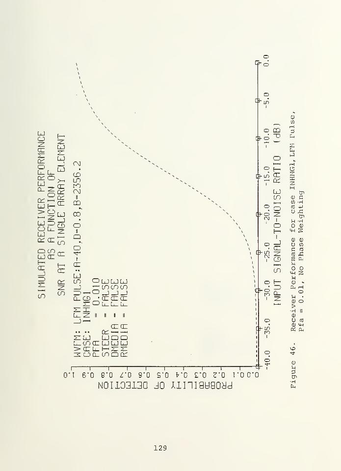
LJCJZce

E-<

LJZcnoL_ L_

LJ_JLJ

CM•

CDIDcn o >-

LJo_ zocn •—

«

LJ E—

CEcncnce

DOf\]

II

CD

> OLJ ZDCJ L_LJcn ce

LJ_jCDzi—

i

CO

CD•

OIIQ

CD COcn

Olj ce

II

E—

<

cn E-<

cn

cn

CE• •

LJCD CD LJLJLJ

z _J '—

1

CD CO CO

CD CO ZD—

<

o _J_J_]Q_CD • CECECE

z: o L_L_L_XZJZL_ z II ii n ii

-j~CECE

• • • cn~~21 LJ LJCDQL_ CO CD LJ LJ LJ>cel_e-<z:z:e< oo_ coocr

o&6

o

O3- o

[*

om

i

[3-

CD"D

E—CEcn

LJCO

CD

[%

Ch

C3-

I

1 1 1 1 1 1 1 1 1 $O'l 6'0 8"0 Z'O 9*0 9*0 ^"0 £'0 2"0 I"0 0*0

N0UG313Q jo uniauGoyd

oE-«

CEzCD

CO

EDQ_

toI

o

0)

rH

pCm

fa

cs

HCD CW >HrO 4J

U JS

U -HCD

CD

uctd

6uomMCD

CM

CD O>H II

CD

rd

CD <WOS cm

Q)

pCn•Hfa

129

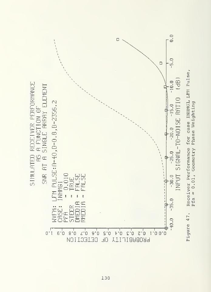
D

LJCDzlaz

LJ21

enoL_ L_

LJ_JLJ e

CDLO

ER

PER

TION

>-i

azenenaz

rooo

ii

CO

RECEIV

fl

EUNC

LJ_jCDzl

CO

ODc

OIIQ

Q COlj az az

Oii

az_jID2Z

E—en

en

az• e

LJCO O LJLJ

zl _] *-; LJCOCOCO CO ZD^-O ZD_]^

Q_CD ' câzazZCCD E-<L_L_

2ZZZU-ZL II II 11 II

—\~azaz

• a • en^^ZILJ L1QDL_COaZLJLJLJ>0ZL_f-'2Z2Zzoo-cnacc

[•

\

\

\

\

\

i i i i i i ~i i i r~

"I 6*0 8"0 Z'O 9*0 5*0 fr'O £'0 Z'O TO 0*0

N0H33I3Q jo umauaoyd

oin

I

E—azen

LJCO

ooro

i

Lh

C3- ml

azZLCD^^CO

E-h

ZDQ_

Bo

CD

r-H

fa

o cS -H3 -Pz .cm rji

HCD (L)

w SU CD

CO

5-1 (0

A4-1 &4

CD >iU ^C 4J

rd 0)

g eM O

CD4-1 OuCD -

01 rHo

u •

CD O>•H ||

CD

U 03

QJ 4-1

PS Oj

r-

CD

5-1

OCn•HCm

130

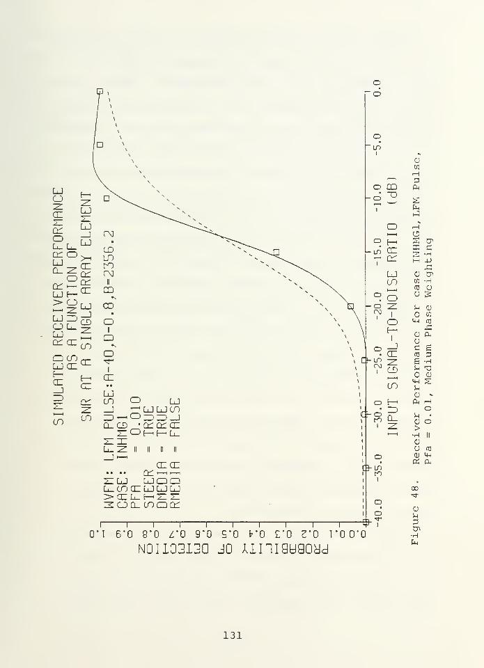
LJCJZZCZ

E-<

ZZLJ\ \

N.

z:enoL_ L_

LJ_lLJ

CDLOcr o >-<

ER

PE

TION

arC£

az

CMii

CD

—H ZZ

LJ ZDCJ L_LJ

LJ_JCDzz

CO

CD•

OIIQ

Q COlj az az

Oii

az_iZDZZ

az

ii

a:• •

LJCO o LJ

zz _] '—

'

LJLJCOCO CO ZD-^ o ZDZD-J

Q_C£) • criczazZZ o E

—' E— Q_

ZZZZL_ZZ II II D II

_J—

<

azen• o • Q^H-H—<

ZZLJ UDDL_ CO 01 LJ LJ LJ> az L_ E-< ZZ 2ZZGCLinDo:

oo

LDI

OO

I

oID

I

oI

CO

L>

Ch

CEcr

LJCO

Oi

azzzCD

CO

f-H

ZDQ_

I 1 1 1 1 1 1 1 1 1 W0*1 6'0 8*0 Z'O 9*0 S"0 fr'O £'0 Z'O I'OO'O

N0I133I3Q JO UHIGUGOyd

[J-LDto

Oo

CD

CO

r—

I

3

fah3

OS CnS3 C£ -HH +J

CL) CnCfi -Hfd mu 5M 0)

o to

4-1 d

a) a,uc03

4-1

UCD

Cm

ii

0)

>•HCD

U as

o 4-j

Oi C4

00^r

CD

S-i

PCn-Hfa

131

Figures 38, 41, 44 and 47 show the receiver performance

when only the system geometry is compensated for by the

phase weights used in the array processor. These figures

indicate that in the presence of the inhomogeneous ocean

medium, phase weighting to compensate for system geometry

will not achieve the receiver performance predicted by

theory. That is, traditional beam steering is not suffi-

cient for maximum receiver performance, and a large margin

for improved performance exists when the effects of the

ocean medium on the received signal can be predicted. Note

also that the degradation in performance is consistent for

the different transmit waveforms and values of Pfa.

Figures 39, 42, 45 and 48 show the effect on receiver

performance when phase weights are computed based on both

the system geometry and the refraction of the acoustic wave

in the ocean medium. The state of the logical variable

DMEDIA indicates if the phase weights contain the correction

for deterministic, inhomogeneous medium wave propagation

effects. As expected, the simulated receiver performance

conforms to the performance predicted by theory, and is

nearly identical to that of case TEST when all medium

effects have been corrected for.

However, the really significant result is seen by com-

paring Figures 38, 41, 44 and 47 with Figures 39, 42, 45 and

48. The only difference between these plots is in use of

phase weights that compensate for the phase shifts due to

132

propagation through an inhomogeneous ocean medium, and the

model of the inhomogeneous ocean medium is based on the

physics of acoustic wave propagation. If one assumes a

marginal detection probability of 50% (Pd = 0.5), the

improvement in receiver performance due to the application

of a model-based signal processing approach for this particu-

lar simulation geometry and ocean medium characteristic

varies from 14 dB to 18 dB depending on the type of

transmit waveform or value of Pfa. The conclusion is that

the physics of wave propagation can be used to develop

signal processing algorithms having significant impact on

the performance of a receiver designed to process complex

envelope, electrical signals from an array of point source

elements

.

133

V. CONCLUSIONS AND RECOMMENDATIONS

The original objectives of this research have been accom-

plished. The computer simulation of a correlator/matched

filter receiver to process data from an array of electro-

acoustic transducers has been developed and validated. The

concept of model-based signal processing was applied to the

development of an array signal processing algorithm, and was

shown to have a marked impact on the capability of the

receiver to detect the presence of a signal in zero-mean,

additive, white Gaussian noise.

The computer simulation of the receiver was validated by

a direct comparison between the measured performance of the

simulation and the performance predicted by theory when all

array element output electrical signals are precisely

cophased. The agreement between predicted and measured

performance was close but not exact since the noise assump-

tions made in developing the theoretical performance could

not be precisely duplicated by the computer simulation.

However, the close agreement with theoretical performance

was considered to be a validation of the receiver simulation

computer program.

Test cases were designed and run that permitted relative

changes in receiver performance to be measured. In this

way, the effectiveness of the model-based signal processing

approach could be quantified. For the simulation parameters

134

and transmit signals used in this study, compensating for

the refraction of the acoustic field in the ocean medium

was found to improve receiver performance over traditional

beam steering by at least 14 dB when measured at the point

of 50% probability of detection.

Suggestions for further study of the receiver model

include

:

- Obtain, or develop, a pseudorandom noise generatorthat more closely approximates the noise modelassumptions implicit in the derivation of thetheoretical receiver performance, and revalidatethe computer simulation.

- Simulate more realistic noise processes, such ascolored noise, and determine the impact on receiverperformance.

- Try decision rules other than Neyman-Pearson, suchas the minimum average probability of error criterionto measure probability of error performance for anunderwater, acoustic data communication system.

- Experiment with other functional forms for thetransmit signal, and measure the effect on perfor-mance when errors in the estimate of time delay andDoppler shift exist.

135

LIST OF REFERENCES

1. Mendel, J., "Model-Based Signal Processing," Trends &

Perspectives in Signal Processing , pp. 9-11, December1983.

2. Ziomek, L.J., Underwater Acoustics--A Linear SystemsTheory Approach , Academic Press, 1985.

3. Vos, J., Linear Time-Invariant, Space-Variant Filtersand the WKB Approximation with Applications toUnderwater Acoustic Signal Processing , Master's Thesis,Naval Postgraduate School, Monterey, California,December 1984.

4. Van Trees, H.L., Detection, Estimation, and ModulationTheory , v. Ill, John Wiley & Sons, Inc., 1971.

5. Couch, L.W. , Digital and Analog Communications Systems ,

Macmillan Publishing Co., 1983.

6. Brigham, O.E., The Fast Fourier Transform , PrenticeHall, Inc. , 1974.

7. Oppenheim, A.V., and Schafer, R.W., Digital SignalProcessing , Prentice Hall, Inc., 1975.

8. Officer, C.B., Introduction to the Theory of SoundTransmission , McGraw-Hill Book Co., 1958.

9. Papoulis, A., Signal Analysis , McGraw-Hill Book Co.,1977.

136

INITIAL DISTRIBUTION LIST

No. Copies

1. Defense Technical Information Center 2

Cameron StationAlexandria, Virginia 22304-6145

2. Library, Code 0142 2


3. Assistant Professor L.J. Ziomek, Code 62Zm 15Department of Electrical and

Computer EngineeringNaval Postgraduate SchoolMonterey, California 93943-5100

4. Commandant (G-TPP/HRP) 2

U.S. Coast Guard Headquarters2100 Second St. S.W.Washington, D.C. 20593

5. LT R.J. Blount . 2

c/o Commanding Officer (MW)

U.S. Coast GuardElectronics Engineering CenterWildwood, New Jersey 08260

6. Mr. Charles Stuart 1

DARPA1400 Wilson Blvd.Arlington, Virginia 22209

137

21"»0«

BlountUnderwater acoustic

model-based signalprocessing applied tothe detection of sig-nals from a planararray of point sourceelements.

Thesis/B569

c.l

21^3Blount

Underwater acoustic

model-based signal

processing applied to

the detection of sig-

nals from a planararray of point source

elements.

**»"*^

w

Documents

Underwater acoustic model-based signal processing applied ... · Calhoun: The NPS Institutional Archive Theses and Dissertations Thesis Collection 1985-09 Underwater acoustic model-based