Understanding Transportation Modes Based on GPS Data … · Understanding Transportation Modes Based on GPS Data ... it is generic to be deployed in a broad range of Web applications

1

Understanding Transportation Modes Basedon GPS Data for Web Applications

YU ZHENG

Microsoft Research Asia

YUKUN CHEN

Tsinghua University

QUANNAN LI

Huazhong University of Science and Technology

and

XING XIE and WEI-YING MA

Microsoft Research Asia

User mobility has given rise to a variety of Web applications, in which the global positioningsystem (GPS) plays many important roles in bridging between these applications and end users.As a kind of human behavior, transportation modes, such as walking and driving, can providepervasive computing systems with more contextual information and enrich a user’s mobility withinformative knowledge. In this article, we report on an approach based on supervised learning toautomatically infer users’ transportation modes, including driving, walking, taking a bus and ridinga bike, from raw GPS logs. Our approach consists of three parts: a change point-based segmentationmethod, an inference model and a graph-based post-processing algorithm. First, we propose achange point-based segmentation method to partition each GPS trajectory into separate segmentsof different transportation modes. Second, from each segment, we identify a set of sophisticatedfeatures, which are not affected by differing traffic conditions (e.g., a person’s direction when in acar is constrained more by the road than any change in traffic conditions). Later, these features arefed to a generative inference model to classify the segments of different modes. Third, we conductgraph-based postprocessing to further improve the inference performance. This postprocessingalgorithm considers both the commonsense constraints of the real world and typical user behaviorsbased on locations in a probabilistic manner. The advantages of our method over the related worksinclude three aspects. (1) Our approach can effectively segment trajectories containing multiple

This article is an expanded version of Zheng et al. [2008], which appears in Proceedings of the 4thInternational Conference on the World Wide Web, 247–256.Authors’ addresses: Y. Zheng, X. Xie, and W. Y. Ma, Microsoft Research Asia, 4F Sigman Build-ing, 49 Zhichun Road, Haidian District, Beijing 100190, China; email: {yuzheng,xingx,wyma}@microsoft.com; Y. Chen, Department of Computer Science, Tsinghua University, Beijing 100084,China; email: [email protected]; Q. Li, Huazhong University of Science and Technology,Wuhan 430074, China.Permission to make digital or hard copies of part or all of this work for personal or classroom useis granted without fee provided that copies are not made or distributed for profit or commercialadvantage and that copies show this notice on the first page or initial screen of a display alongwith the full citation. Copyrights for components of this work owned by others than ACM must behonored. Abstracting with credit is permitted. To copy otherwise, to republish, to post on servers,to redistribute to lists, or to use any component of this work in other works requires prior specificpermission and/or a fee. Permissions may be requested from Publications Dept., ACM, Inc., 2 PennPlaza, Suite 701, New York, NY 10121-0701 USA, fax +1 (212) 869-0481, or [email protected]© 2010 ACM 1559-1131/2010/01-ART1 $10.00DOI 10.1145/1658373.1658374 http://doi.acm.org/10.1145/1658373.1658374

ACM Transactions on The Web, Vol. 4, No. 1, Article 1, Publication date: January 2010.

1:2 • Y. Zheng et al.

transportation modes. (2) Our work mined the location constraints from user-generated GPS logs,while being independent of additional sensor data and map information like road networks andbus stops. (3) The model learned from the dataset of some users can be applied to infer GPS datafrom others. Using the GPS logs collected by 65 people over a period of 10 months, we evaluatedour approach via a set of experiments. As a result, based on the change-point-based segmentationmethod and Decision Tree-based inference model, we achieved prediction accuracy greater than71 percent. Further, using the graph-based post-processing algorithm, the performance attained a4-percent enhancement.

Categories and Subject Descriptors: I.5.2 [Pattern Recognition]: Design Methodology—Classifierdesign and evaluation; H.2.8 [Database Management]: Database Applications—Data mining

General Terms: Algorithm, Design, Experimentation

Additional Key Words and Phrases: Spatial data mining, GPS trajectory, ubiquitous computing,understanding user behavior, GeoLife, user mobility, transportation modes

ACM Reference Format:Zheng, Y., Chen, Y., Li, Q., Xie, X., and Ma, W.-Y. 2010. Understanding transportation modes basedon GPS data for Web applications. ACM Trans. Web, 4, 1, Article 1 (January 2010), 36 pages.DOI = 10.1145/1658373.1658374 http://doi.acm.org/10.1145/1658373.1658374

1. INTRODUCTION

The increasing pervasiveness of location-acquisition technologies, such as GPSand GSM network, is leading to the large collection of spatio-temporal datasets.Such datasets have supported a variety of novel Web applications, in which lo-cality and mobility usually connect to one another closely. For instance, peoplecan tag user-generated contents like photos with locations [Toyama et al. 2003];trace their outdoor mobility [Ashbrook and Starner 2003]; and use location-based services [Chen and Kotz 2000]. Recently, a branch of GPS-track-sharingapplications using Web maps appeared on the Internet. In this category of Webapplications [Counts and Smith 2007], people can record their travel routes us-ing a GPS-equipped device and then share travel experiences among each otherby publishing these GPS tracks in a Web community. GPS-track-sharing offer amore fancy and interactive approach than text-based articles to better expresspeople’s travel experiences, which provide users with valuable references whenplanning a travel itinerary.

However, so far, these applications require people either to manually la-bel their own trajectories or to use raw GPS data such as GPS coordinatesand timestamps without much understanding. Neither of these methods is op-timal to the development of such applications. Actually, users become easilyfrustrated by the additional data-labeling effort, and then give up uploadingtheir data. Moreover, people intend to understand an individual’s mobility, andlearn information about user behaviors as well as user intentions behind theraw data.

Being an important kind of human behavior, transportation modes, such aswalking, driving, and taking a bus, can enrich their mobility with knowledgeand provide pervasive computing systems with more contexts.

—For users. The information of transportation modes helps individuals ef-fectively reflect on their past events, and deeply understand their own life


Understanding Transportation Modes Based on GPS Data • 1:3

pattern as well. Also, with the transportation modes of a GPS track, peopleare facilitated to share life experience among each other in Web communi-ties, and obtain more reference knowledge from others’ trajectories. Userscan know not only where other people have been but also how these peoplereach each location.

—For the service providers. Such knowledge enables the application systemsto classify GPS tracks into different categories of transportation mode.Therefore, systems are capable of performing smart route recommenda-tions/designs for a person based on the person’s needs. For instance, a systemshould return a bus line rather than a driving route to an individual intend-ing to move to somewhere by a bus.

Moreover, a transportation mode can feature many pervasive computing sys-tems aiming to recognize human activities from GPS data. Such high-levelactivities would both enable the creation of new computing services that au-tonomously respond to a person’s unspoken needs and support more accuratepredictions about future behaviors, such as moving direction [Liao et al. 2004],destination [Krumm et al. 2003], and life pattern [Patterson et al 2003]. In turn,the knowledge learned from these works can be leveraged to further enhancemany innovative local/mobile applications on the Web.

Unfortunately, the identification methods based on simple rules, such as avelocity-based approach, cannot handle this problem with great effect due to thefollowing reasons: 1) people usually change their transportation modes duringa trip, that is, a GPS trajectory may contain multiple modes. 2) The velocity ofdifferent transportation modes is usually vulnerable to traffic conditions andweather. Intuitively, in congestion, the mean velocity of driving would be asslow as riding a bike.

In this article, we aim to automatically infer transportation modes, includingdriving, walking, taking a bus, and riding a bicycle, from raw GPS logs basedon supervised learning. It is a step toward recognizing human behavior andunderstanding user mobility for pervasive computing systems. Also, it is a steptoward improving local/mobile applications on the Web and enhancing the con-nection between mobility and locality by mining knowledge from raw GPS datawith minimal user efforts. The contributions of this work lie in the followingthree areas.

First, we propose a change point-based segmentation method. This methodaims to partition each GPS trajectory into separate segments of different trans-portation modes, while maintaining a segment of one mode as long as possible.In addition, this segmentation method is capable of enhancing the reliabilityof our methodology facing the variable traffic conditions.

Second, from each segment, we identify a set of sophisticated features, suchas direction change rate, velocity change rate, and stop rate. These features havefew correlations with the velocity, hence are not affected by differing traffic con-ditions. These set of features can also be extended to other pervasive computingsystems aiming to recognize human behavior and understand user mobility.

Third, we conduct a graph-based postprocessing algorithm to further im-prove the inference performance. In this algorithm, we mine the commonsense



constraints of the real world and typical user behaviors on a location from user-generated GPS logs. Therefore, we are able to leverage this location-constrainedknowledge as probabilistic cues, while maintaining our methodology being in-dependent of an additional database of road networks or points of interests.

Overall, the advantages of our method over the related works include twoparts. (1) Our method is independent of other sensor data like GSM signal andheart rate, and map information, for example, road networks and bus stops,etc. Thus, it is generic to be deployed in a broad range of Web applications. 2)The model learned from the dataset of some users can be applied to infer GPSdata from others; that is, it is not a user-specific model.

The rest of this article is organized as follows. In Section 2, we justify themotivation of inferring transportation mode using two application scenarios.Section 3 first describes the framework of our approach, and then introduceseach component of the proposed method in details. In Section 4, we conduct a setof experiments, which evaluate our approach based on a GPS dataset collectedby 65 people over a period of 10 months. The major experimental results, aswell as the corresponding discussion, are also reported here. Finally, after in-troducing some related works in Section 5, we draw our conclusion in Section 6.

2. APPLICATION SCENARIOS

The work reported in this article is a part of research into our project GeoLife,which focuses on lively visualization [Zheng et al. 2008c, 2008d], fast retrieval[Wang et al. 2008] and a deep understanding [Zheng et al. 2008a, 2008b] of GPStrack logs for both personal and public use. Our approach has been deployedin the website of GeoLife to automatically tag transportation modes to GPStracks submitted by users. Leveraging the following two cases, we differentiatebetween the significance of a GPS track with and without the information oftransportation modes.

2.1 Improving Sharing and Interactions between Users

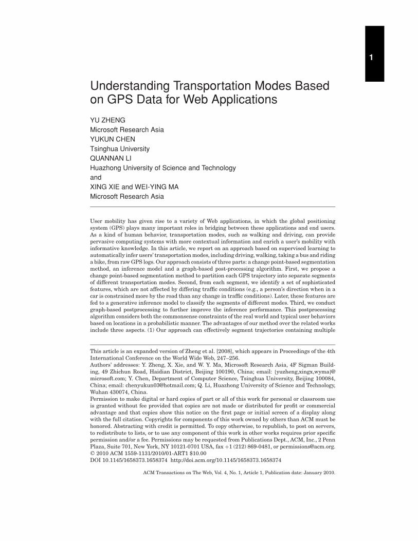
Using a GPS trajectory generated by an individual, Figure 1 presents an ex-ample to distinguish the different Web experiences with and without trans-portation modes. Without the tag of transportation modes, the track shown inthe Figure 1(a) provides us nothing but a ploy-line. However, as illustrated inFigure 1(b) and (c), after conducting inference, we realize that the individualfirst drives downtown, and then switches to walking at a parking lot. Based onthis observation, a place where we are allowed to park a car was discovered,and how long we might spend on the way by driving was correctly suggested.Meanwhile, this track may also offer a reference experience to walking down-town from the parking lot. In this way, we are more likely to avoid heavy traffic,and enjoy shopping when passing the street side. Regardless of the fact thatthis track is a compound trajectory containing driving and walking, the meanvelocity of the whole track would be quite slow given the relatively long dura-tion consumed by walking. Therefore, the route might be deemed as a way thatsuffered from heavy traffic. In other words, we might ignore it when searchingfor an efficient way to drive downtown.



Fig. 1. An example of inferring transportation modes from raw GPS data.

Fig. 2. Route recommendation according to users’ preferences on transportation modes.

2.2 GPS Trajectories Classification

Using a set of GPS trajectories generated in the real world, Figure 2 furtherdemonstrates the contribution of our work to route planning/recommendationsystems. In Figure 2 (a), there are many route candidates for our selection whenwe attempt to find a way from the bottom right to the top left. Intuitively, peo-ple have various preferences on transportation modes when planning a travelroute. For instance, some individuals like riding a bike, while others prefer



Fig. 3. GPS log, segment and change point.

driving or taking buses. Unfortunately, these routes are less discriminativefrom one another before being inferred. Actually, as shown in Figure 2(b), theseroutes are generated by different users taking different transportation modes,such as driving and riding a bike. Thus, if a user wants to ride a bike to their des-tination, we should recommend the route shown in Figure 2(c). Likewise, whenthe person needs to drive, we should present the route depicted in Figure 2(d).

3. INFER TRANSPORTATION MODES

In this section, we first define some preliminary concept about GPS data, andthen give an overview on the framework of our methodology. Subsequently, thefour steps, consisting of segmentation, feature extraction, inference and post-processing, of our approach are respectively described in detail.

3.1 Preliminary

Before describing the framework of our approach, we have to define the fol-lowing terms: GPS log, GPS trajectory, Walk Segment, non-Walk Segment, andchange point. Basically, as depicted in the left part of Figure 3, a GPS log is a se-quence of GPS points, pi ∈ P , P = {p1, p2, . . . , pn}. Each GPS point pi containslatitude, longitude and a timestamp. On a two dimensional plane, we can se-quentially connect these GPS points into a GPS trajectory, and then divide theGPS trajectory into trips if the time interval between the consecutive pointsexceeds a certain threshold. A change point stands for a place where a userchanges their transportation mode in a trajectory. For instance, in the rightpart of Figure 3, a change point was generated when an individual transferredfrom driving to walking.

For simplicity’s sake, we name the segments users traveled on foot as WalkSegments, while the segments of other transportation modes are called non-Walk Segments. Further, we call the GPS point from a Walk Segment, suchas Pn−1, a Walk Point, while the GPS points like P2 from non-Walk Segmentsare coined in non-Walk Points. In short, as depicted in Figure 3, a trip can bepartitioned into a Walk Segment and a non-Walk Segment by a change pointwhere the user transfers from driving to walking. In the remainder of thisarticle, we use {Bike, Bus, Driving, Walk} to respectively represent the followingfour kinds of transportation modes: riding a bike; taking a bus; driving or takinga taxi; traveling on foot.

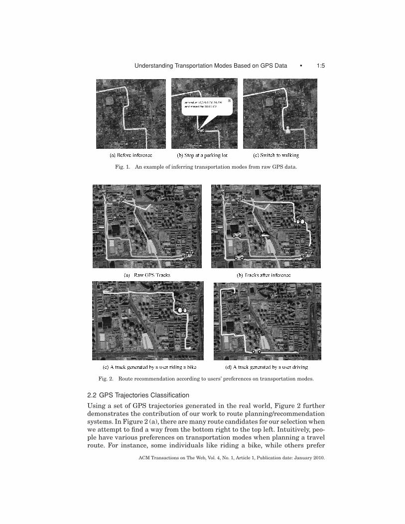
Figure 4 depicts how we calculate features from GPS logs. Given two con-secutive GPS points, for example, p1 and p2, we can calculate the spatial dis-tance L1, temporal interval T1 and heading direction (p1.head) between them.



Fig. 4. Feature calculation based on GPS logs.

Fig. 5. Architecture of our approach.

Subsequently, the velocity of p1 can be computed as Equation (1).

p1.V1 = L1/T1. (1)

Then, the heading change, such as H1,of three consecutive points like p1, p2and p3 can be calculated as Equation (2).

H1 = |p1.head − p2.head|. (2)

Further, more features, such as acceleration and expectation of velocity, can becalculated in this manner.

3.2 Architecture of Our Approach

As shown in Figure 5, the architecture of our approach includes two parts,offline learning and online inference.

In the offline learning section, on one hand, we first partition GPS trajectoriesinto segments based on change points and extract features from each segment.Then, the features and corresponding ground truths are employed to train aclassification model for online inference.

On the other hand, using a density-based clustering algorithm, we groupthe change points detected from all users’ GPS logs into clusters. Subsequently,a graph based on these clusters and user-generated GPS trajectories is built.



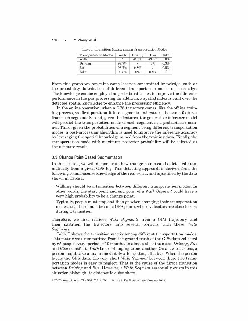
Table I. Transition Matrix among Transportation Modes

Transportation Modes Walk Driving Bus BikeWalk / 41.0% 49.0% 9.0%Driving 99.7% / 0% 0.3%Bus 98.7% 0.8% / 0.5%Bike 99.8% 0% 0.2% /

From this graph we can mine some location-constrained knowledge, such asthe probability distribution of different transportation modes on each edge.The knowledge can be employed as probabilistic cues to improve the inferenceperformance in the postprocessing. In addition, a spatial index is built over thedetected spatial knowledge to enhance the processing efficiency.

In the online operation, when a GPS trajectory comes, like the offline train-ing process, we first partition it into segments and extract the same featuresfrom each segment. Second, given the features, the generative inference modelwill predict the transportation mode of each segment in a probabilistic man-ner. Third, given the probabilities of a segment being different transportationmodes, a post-processing algorithm is used to improve the inference accuracyby leveraging the spatial knowledge mined from the training data. Finally, thetransportation mode with maximum posterior probability will be selected asthe ultimate result.

3.3 Change Point-Based Segmentation

In this section, we will demonstrate how change points can be detected auto-matically from a given GPS log. This detecting approach is derived from thefollowing commonsense knowledge of the real world, and is justified by the datashown in Table I.

—Walking should be a transition between different transportation modes. Inother words, the start point and end point of a Walk Segment could have avery high probability to be a change point.

—Typically, people must stop and then go when changing their transportationmodes, i.e., there must be some GPS points whose velocities are close to zeroduring a transition.

Therefore, we first retrieve Walk Segments from a GPS trajectory, andthen partition the trajectory into several portions with these WalkSegments.

Table I shows the transition matrix among different transportation modes.This matrix was summarized from the ground truth of the GPS data collectedby 65 people over a period of 10 months. In almost all of the cases, Driving, Busand Bike transfer to Walk before changing to one another. On a few occasions, aperson might take a taxi immediately after getting off a bus. When the personlabels the GPS data, the very short Walk Segment between these two trans-portation modes is easy to neglect. That is the cause of the direct transitionbetween Driving and Bus. However, a Walk Segment essentially exists in thissituation although its distance is quite short.



0%

2%

4%

6%

8%

10%

12%

14%

16%

18%

1 2 3 4 5 6 7 8 9 10 11 12 13 14 15 16 17 18 19 20 21 22 23 24 25 26 27 28 29 30 31 32 33 34

Per

cent

age

The maximal velocity (m/s)

Walk

Bike

Bus

Driving

Fig. 6. The distribution of the maximum velocity of a segment.

0%

10%

20%

30%

40%

50%

60%

0 1 2 3 4 5 6 7 8 9 10 11 12 13 14 15 16 17 18 19 20

Per

cent

age

Average Speed(m/s)

Walk

Bike

Bus

Driving

Fig. 7. The distribution of the average speed of a segment.

However, over the same dataset, Figures 6, 7, and 8 respectively show thedistribution of maximum velocity, average velocity and maximum accelerationof different transportation modes. The data shown in these figures paints a richpicture about how difficult it is to give some simple rules to directly distinguishbetween the segments of different transportation modes. Without knowing howmany modes a trip contains, it is especially difficult to tackle the problem usingsimple rules.

Enlightened by the previously-mentioned commonsense knowledge as wellas the information mined from GPS data, we first find the change points bydetecting Walk Segments from a trip. Then, using these change points, we areable to partition the trip into alternate Walk Segments and non-Walk Segments.Since segments from a trip are first categorized into two classes {Walk, non-Walk} rather than four classes {Bike, Bus, Driving, Walk}, the complexity ofsegmentation has been reduced greatly. Subsequently, we can extract the fea-tures of each segment and further infer its specific transportation mode. Using



0%

5%

10%

15%

20%

25%

30%

35%

40%

0 1 2 3 4 5 6 7 8 9 10

Per

cent

age

The Maximal Acceleration(m/s2)

Walk

Bike

Bus

Driving

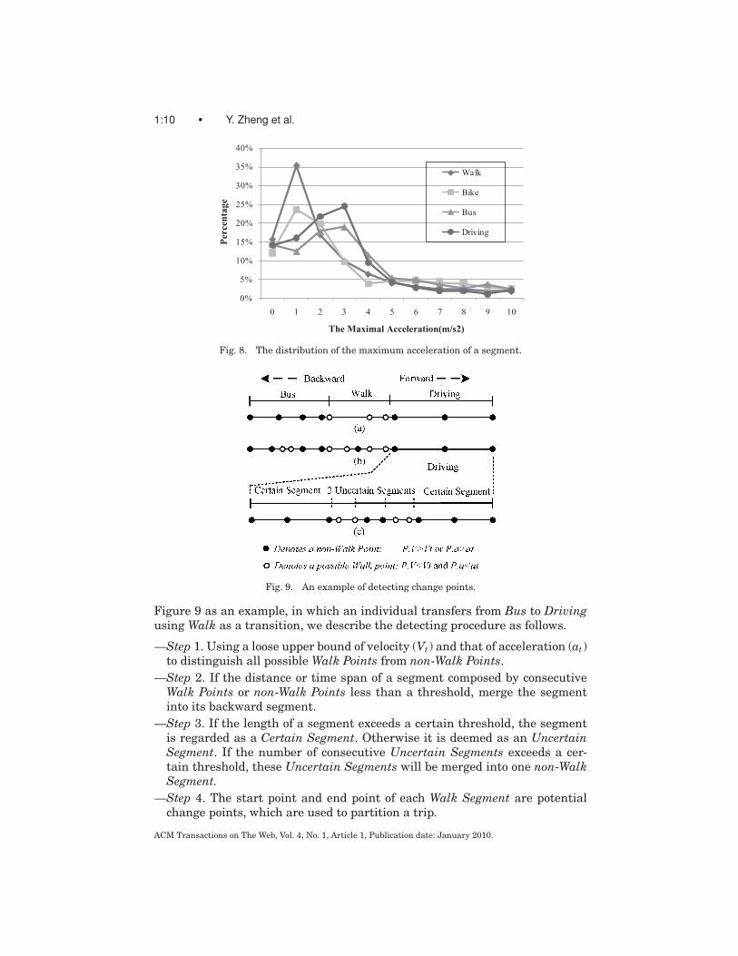
Fig. 8. The distribution of the maximum acceleration of a segment.

Fig. 9. An example of detecting change points.

Figure 9 as an example, in which an individual transfers from Bus to Drivingusing Walk as a transition, we describe the detecting procedure as follows.

—Step 1. Using a loose upper bound of velocity (Vt) and that of acceleration (at)to distinguish all possible Walk Points from non-Walk Points.

—Step 2. If the distance or time span of a segment composed by consecutiveWalk Points or non-Walk Points less than a threshold, merge the segmentinto its backward segment.

—Step 3. If the length of a segment exceeds a certain threshold, the segmentis regarded as a Certain Segment. Otherwise it is deemed as an UncertainSegment. If the number of consecutive Uncertain Segments exceeds a cer-tain threshold, these Uncertain Segments will be merged into one non-WalkSegment.

—Step 4. The start point and end point of each Walk Segment are potentialchange points, which are used to partition a trip.



As depicted in Figure 9, each possible Walk Point (white points) is a GPS pointwhose velocity (P.V ) and acceleration (P.a) are both smaller than the givenbound. Ideally, as demonstrated in Figure 9(a), only one Walk Segment wouldbe detected from this trip. However, as illustrated in Figure 9(b), when a vehiclemoves slowly in some transient occasions, a few GPS points from non-WalkSegments may be detected as possible Walk Points. Also, because of the locativeerror, a few points from the Walk Segment will exceed the bound, and becomenon-Walk Points (black points in Figure 9). To improve the precision of thesegmentation method, we require that the distance of each retrieved segmentmust exceed a certain distance. Otherwise, it will be merged into its backwardsegment. For instance, in Figure 9(b), the two Walk Points contained in theBus segment cannot construct a stand-alone segment due to the short distancebetween them. Therefore, it will be merged into its backward segment. Thesame criterion is also applied to handle the outlier points in Walk Segment.

After step 1 and step 2 are conducted, the trip is partitioned into a se-ries of alternate Walk Segments and non-Walk Segments. As demonstrated inFigure 9(c), unfortunately, in some occasions, in which a user meets conges-tion or heavy traffic, a Driving segment may be composed of many alternateWalk Segments and non-Walk Segments. It is not appropriate for the classifica-tion model to conduct inference using the features extracted from such trivialsegments. Intuitively, the longer a segment is the more accurate features a seg-ment might express. Thus, we are more likely to infer its transportation modecorrectly. However, the shorter a segment is, the higher the uncertainty mightbe.

To avoid a trivial partition, which will lead to further inference errors, wetake the following policy to merge, to some extent, the consecutive UncertainSegments. We define a segment whose length exceeds a threshold (e.g., 200 me-ters used in the experiments) as a Certain Segment. Otherwise, we deem it asan Uncertain Segment. In other words, we are not sure about the transporta-tion mode of this segment even if it holds the condition of a Walk Segment. Ifthe number of consecutive Uncertain Segments exceeds a certain threshold, forexample, two we find out in experiments, we still deem all these Uncertain Seg-ments as one non-Walk Segment. It is not difficult to understand that commonusers will not frequently change their transportation modes within such a shortdistance. For instance, as depicted in Figure 9(c), within a certain distance, itis impossible for a person to take the following transition, Driving → Walk →Driving → Walk → Driving. So, we believe the three segments between the twoCertain Segments are also non-Walk Segments, Driving here. Thus, we are ableto merge these Uncertain Segments into one segment and perform a further in-ference. By maintaining the consecutive GPS points of the same transportationmode in one segment, we are more likely to reduce the affection caused by thecongestion.

3.4 Feature Extraction

Table II shows the features we extracted from each segment. Two categoriesof features including Basic Features and Advanced Features are identified.



Table II. The Features We Explored in the Experiment

Category Features SignificanceDist Distance of a segmentMaxVi The ith maximal velocity of a segment

Basic Features MaxAi The ith maximal acceleration of a segmentAV Average velocity of a segmentEV Expectation of velocity of GPS points in a segmentDV Variance of velocity of GPS points in a segmentHCR Heading Change Rate

Advanced Features SR Stop RateVCR Velocity Change Rate

Fig. 10. Heading change rate of different modes.

Following the way we presented in Figure 3 and Figure 4, the Basic Featuresare easily calculated, while the Advanced Features is described in the followingsections. Beyond the Basic Features, the Advanced Features is more robust tovariable traffic conditions.

3.4.1 Heading Change Rate (HCR). As shown in Figure 10, typically, beingconstrained by a road, people driving a car or taking a bus cannot change theirheading direction as flexibly as if they are walking or cycling, no matter whattraffic conditions they meet. Moreover, regardless of traffic conditions and theweather, people walking or riding a bicycle inevitably and unintentionally windtheir way to a destination, although they attempt to create a straight route.

In other words, the heading directions of different transportation modes dif-fer greatly in being constrained by the real routes while being independent oftraffic conditions. Thus, HCR modeling this principle is defined as Equation (3).

HCR = |Pc|/Distance, (3)

where Pc stands for the collection of GPS points at which a user changes his/herheading direction exceeding a certain threshold (Hc). |Pc| represents the num-ber of elements in Pc. After dividing |Pc| by the distance of the segment, HCRcan be regarded as the frequency that people change their heading direction tosome extent within a unit distance.

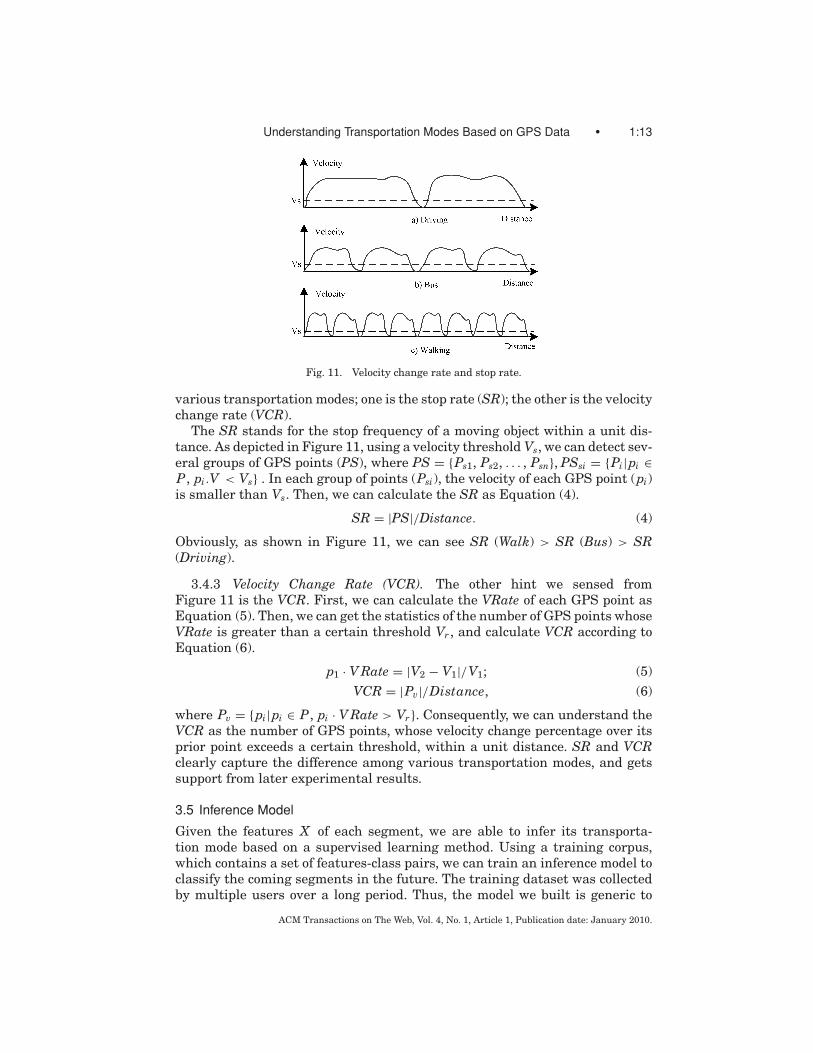
3.4.2 Stop Rate (SR). Figure 11 presents the typical trend of velocity whenpeople take different transportation modes. We observe that, within a similardistance, people taking a bus are likely to stop more times than driving. Intrin-sically, besides waiting at traffic lights, a bus would take passengers on or off atbus stops. Meanwhile, people walking on a route would become more likely thanthey would in other modes to stop somewhere on their journey, such as whentalking with passersby, being attracted by surrounding environments, waitingfor a bus. These observations motivate us to define two features to differentiate



Fig. 11. Velocity change rate and stop rate.

various transportation modes; one is the stop rate (SR); the other is the velocitychange rate (VCR).

The SR stands for the stop frequency of a moving object within a unit dis-tance. As depicted in Figure 11, using a velocity threshold Vs, we can detect sev-eral groups of GPS points (PS), where PS = {Ps1, Ps2, . . . , Psn}, PSsi = {Pi|pi ∈P, pi.V < Vs} . In each group of points (Psi), the velocity of each GPS point (pi)is smaller than Vs. Then, we can calculate the SR as Equation (4).

SR = |PS|/Distance. (4)

Obviously, as shown in Figure 11, we can see SR (Walk) > SR (Bus) > SR(Driving).

3.4.3 Velocity Change Rate (VCR). The other hint we sensed fromFigure 11 is the VCR. First, we can calculate the VRate of each GPS point asEquation (5). Then, we can get the statistics of the number of GPS points whoseVRate is greater than a certain threshold Vr , and calculate VCR according toEquation (6).

p1 · V Rate = |V2 − V1|/V1; (5)VCR = |Pv|/Distance, (6)

where Pv = {pi|pi ∈ P, pi · V Rate > Vr}. Consequently, we can understand theVCR as the number of GPS points, whose velocity change percentage over itsprior point exceeds a certain threshold, within a unit distance. SR and VCRclearly capture the difference among various transportation modes, and getssupport from later experimental results.

3.5 Inference Model

Given the features X of each segment, we are able to infer its transporta-tion mode based on a supervised learning method. Using a training corpus,which contains a set of features-class pairs, we can train an inference model toclassify the coming segments in the future. The training dataset was collectedby multiple users over a long period. Thus, the model we built is generic to



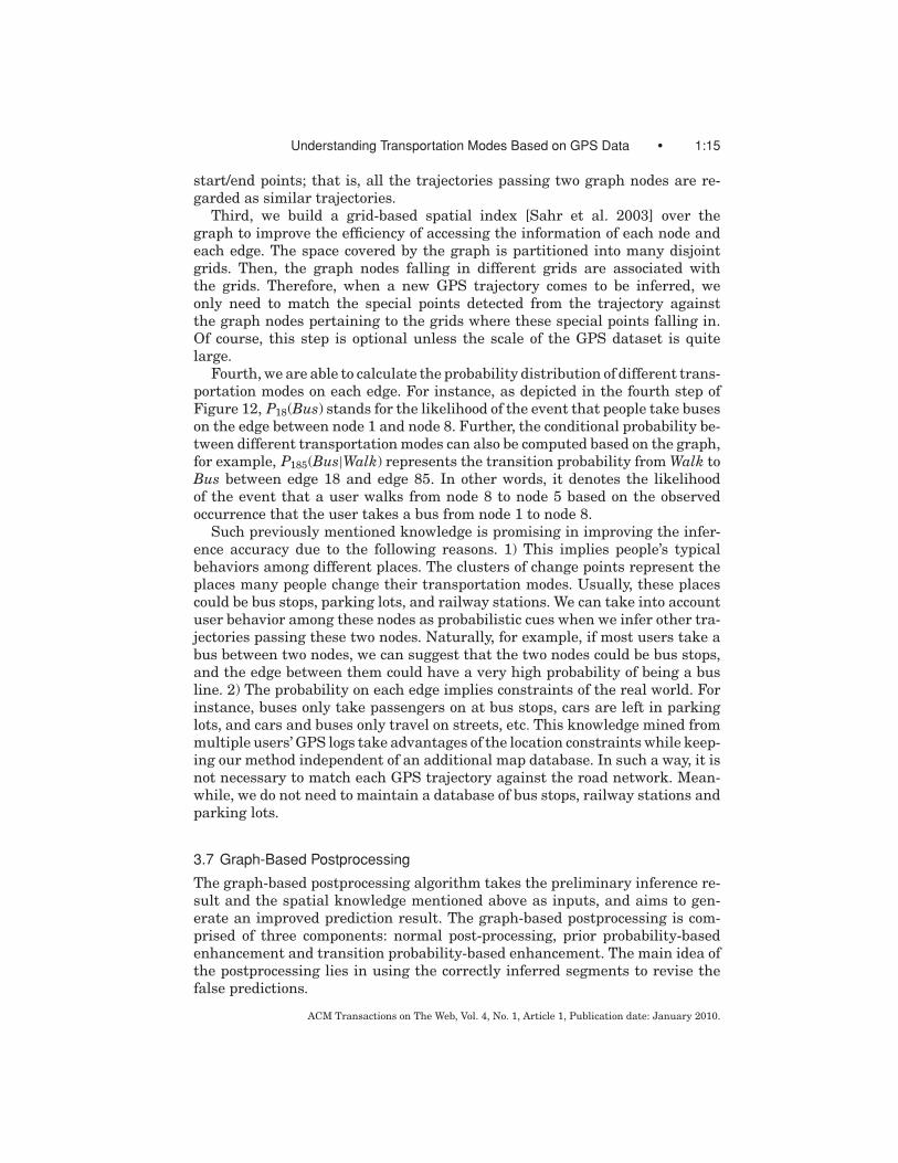
Fig. 12. Mining spatial knowledge from GPS logs.

infer the GPS trajectories for a variety of people. A group of classification algo-rithms, including a Decision Tree, a Support Vector Machine, a Bayesian Net,and a Conditional Random Field, have been tested in our previous experiments[Zheng et al. 2008a]. The results show that the Decision Tree outperforms oth-ers based on the change point-based segmentation. Consequently, we still usethis inference model in this article. Meanwhile, a Bootstrap aggregating (bag-ging) [Breiman 1996] is employed as a meta-algorithm to improve the accuracyof the model by reducing variance and overfitting.

3.6 Spatial Knowledge Extraction

Figure 12 illustrates the four steps toward mining spatial knowledge from users’GPS logs. The knowledge includes a change point-based graph and the proba-bility distribution on each edge of the graph.

First, given GPS logs with labeled ground truths, we can get the specialpoints consisting of change points and the start/end points of each GPS trajec-tory. These special points were subsequently grouped into several nodes (clus-ters) using a density-based clustering algorithm. The reasons we prefer to usedensity-based clustering instead of agglomerative methods, such as K-Means,lie in two aspects. First, a density-based approach is capable of detecting clus-ters with irregular structures, which may stand for bus stops or parking places.Second, it can discover popular places where most people change their trans-portation modes while removing sparse change points representing places withlow access frequency.

Second, with the GPS trajectories from multiple users’ GPS logs, we canconstruct an undirected graph. In such a graph, a node represents a cluster ofthe special points mentioned above, and an edge denotes users’ transitions be-tween two nodes. Here, we do not differentiate various trajectories with similar



start/end points; that is, all the trajectories passing two graph nodes are re-garded as similar trajectories.

Third, we build a grid-based spatial index [Sahr et al. 2003] over thegraph to improve the efficiency of accessing the information of each node andeach edge. The space covered by the graph is partitioned into many disjointgrids. Then, the graph nodes falling in different grids are associated withthe grids. Therefore, when a new GPS trajectory comes to be inferred, weonly need to match the special points detected from the trajectory againstthe graph nodes pertaining to the grids where these special points falling in.Of course, this step is optional unless the scale of the GPS dataset is quitelarge.

Fourth, we are able to calculate the probability distribution of different trans-portation modes on each edge. For instance, as depicted in the fourth step ofFigure 12, P18(Bus) stands for the likelihood of the event that people take buseson the edge between node 1 and node 8. Further, the conditional probability be-tween different transportation modes can also be computed based on the graph,for example, P185(Bus|Walk) represents the transition probability from Walk toBus between edge 18 and edge 85. In other words, it denotes the likelihoodof the event that a user walks from node 8 to node 5 based on the observedoccurrence that the user takes a bus from node 1 to node 8.

Such previously mentioned knowledge is promising in improving the infer-ence accuracy due to the following reasons. 1) This implies people’s typicalbehaviors among different places. The clusters of change points represent theplaces many people change their transportation modes. Usually, these placescould be bus stops, parking lots, and railway stations. We can take into accountuser behavior among these nodes as probabilistic cues when we infer other tra-jectories passing these two nodes. Naturally, for example, if most users take abus between two nodes, we can suggest that the two nodes could be bus stops,and the edge between them could have a very high probability of being a busline. 2) The probability on each edge implies constraints of the real world. Forinstance, buses only take passengers on at bus stops, cars are left in parkinglots, and cars and buses only travel on streets, etc. This knowledge mined frommultiple users’ GPS logs take advantages of the location constraints while keep-ing our method independent of an additional map database. In such a way, it isnot necessary to match each GPS trajectory against the road network. Mean-while, we do not need to maintain a database of bus stops, railway stations andparking lots.

3.7 Graph-Based Postprocessing

The graph-based postprocessing algorithm takes the preliminary inference re-sult and the spatial knowledge mentioned above as inputs, and aims to gen-erate an improved prediction result. The graph-based postprocessing is com-prised of three components: normal post-processing, prior probability-basedenhancement and transition probability-based enhancement. The main idea ofthe postprocessing lies in using the correctly inferred segments to revise thefalse predictions.



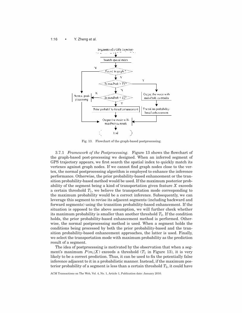
Fig. 13. Flowchart of the graph-based postprocessing.

3.7.1 Framework of the Postprocessing. Figure 13 shows the flowchart ofthe graph-based post-processing we designed. When an inferred segment ofGPS trajectory appears, we first search the spatial index to quickly match itsvertexes against graph nodes. If we cannot find graph nodes close to the ver-tex, the normal postprocessing algorithm is employed to enhance the inferenceperformance. Otherwise, the prior probability-based enhancement or the tran-sition probability-based method would be used. If the maximum posterior prob-ability of the segment being a kind of transportation given feature X exceedsa certain threshold T1, we believe the transportation mode corresponding tothe maximum probability would be a correct inference. Subsequently, we canleverage this segment to revise its adjacent segments (including backward andforward segments) using the transition probability-based enhancement. If thesituation is opposed to the above assumption, we will further check whetherits maximum probability is smaller than another threshold T2. If the conditionholds, the prior probability-based enhancement method is performed. Other-wise, the normal postprocessing method is used. When a segment holds theconditions being processed by both the prior probability-based and the tran-sition probability-based enhancement approaches, the latter is used. Finally,we select the transportation mode with maximum probability as the predictionresult of a segment.

The idea of postprocessing is motivated by the observation that when a seg-ment’s maximum P (mi|X ) exceeds a threshold (T1 in Figure 13), it is verylikely to be a correct prediction. Thus, it can be used to fix the potentially falseinference adjacent to it in a probabilistic manner. Instead, if the maximum pos-terior probability of a segment is less than a certain threshold T2, it could have



Fig. 14. Performing normal post-processing on a GPS trajectory.

a very high probability of being a false inference. Consequently, it deservesour revision. With the threshold T1 and T2, we are more likely to correct thefalse prediction while maintaining accurate inference results. (See Figure 29 forevidences.)

3.7.2 Normal Postprocessing. Normal post-processing aims to improve theprediction accuracy by considering the conditional probability between differenttransportation modes. Using the trajectory depicted in Figure 14 as an exam-ple, we introduce the normal post-processing algorithm. After implementingthe preliminary inference, we can get the predicted posterior probability ofeach segment being different transportation modes given feature X . If we di-rectly select the transportation mode with maximum posterior probability asthe final result, the prediction would be Driving→Bike→Bike, while the groundtruth is Driving→Walk→Bike; that is, a prediction error occurred. On this oc-casion, if a segment, for example, segment[i − 1], whose posterior probabilitybeing a kind of transportation mode exceeds threshold T1 (0.6 used in our ex-periment), we select the transportation mode as the final prediction. Later, ifthe probability of its adjacent segments, for example, segment[i], is less than athreshold T2, the inference of segment[i−1] can be used to revise the predictionof segment[i]. Therefore, the posterior probability of segment[i] being differenttransportation modes conditioned by the transportation mode of segment[i−1]can be re-calculated according to Equations (7) and (8).

Segment[i].P (Bike) = Segment[i].P (Bike) × P (Bike|Driving), (7)Segment[i].P (Walk) = Segment[i].P (Walk) × P (Walk|Driving) (8). . . . .

Here P (Bike|Driving) stands for the probability of an event that a person di-rectly transfers transportation modes from driving to riding a bike. Likewise,P (Walk|Driving) denotes the transition probability from Driving to Walking. Asshown in Table I, these probabilities can be summarized from the user-labeleddata. Segment[i].P (Bike), which represents the probability of the segment[i]being a Bike segment, is the output of the inference model.

After the calculation, we use the transportation mode with maximum prob-ability as the final result. In the case depicted in Figure 14, since the tran-sition probability from Driving to Bike is very small, Segment[i].P (Bike)will drop behind Segment[i].P (Walk) after the multiplications shown in



Fig. 15. Prior probability-based enhancement method.

Equations (7) and (8). In other words, the inference result of Bike will be sub-stituted with Walk. Consequently, a false inference is revised based on thecorrect prediction of its adjacent segment. The normal postprocessing is per-formed in a propagated manner until the conditions (T1 and T2) are not held anylonger.

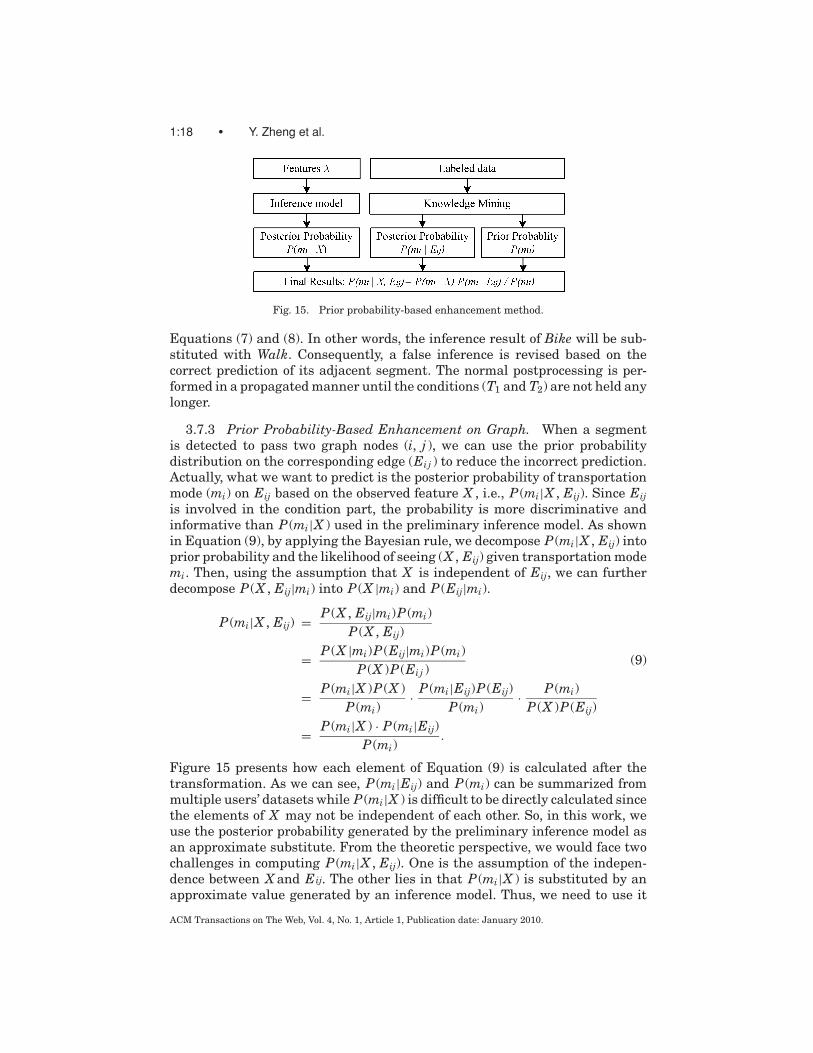
3.7.3 Prior Probability-Based Enhancement on Graph. When a segmentis detected to pass two graph nodes (i, j ), we can use the prior probabilitydistribution on the corresponding edge (Eij ) to reduce the incorrect prediction.Actually, what we want to predict is the posterior probability of transportationmode (mi) on Eij based on the observed feature X , i.e., P (mi|X , Eij). Since Eijis involved in the condition part, the probability is more discriminative andinformative than P (mi|X ) used in the preliminary inference model. As shownin Equation (9), by applying the Bayesian rule, we decompose P (mi|X , Eij) intoprior probability and the likelihood of seeing (X , Eij) given transportation modemi. Then, using the assumption that X is independent of Eij, we can furtherdecompose P (X , Eij|mi) into P (X |mi) and P (Eij|mi).

P (mi|X , Eij) = P (X , Eij|mi)P (mi)P (X , Eij)

= P (X |mi)P (Eij|mi)P (mi)P (X )P (Eij )

(9)

= P (mi|X )P (X )P (mi)

· P (mi|Eij)P (Eij)P (mi)

· P (mi)P (X )P (Eij)

= P (mi|X ) · P (mi|Eij)P (mi)

.

Figure 15 presents how each element of Equation (9) is calculated after thetransformation. As we can see, P (mi|Eij) and P (mi) can be summarized frommultiple users’ datasets while P (mi|X ) is difficult to be directly calculated sincethe elements of X may not be independent of each other. So, in this work, weuse the posterior probability generated by the preliminary inference model asan approximate substitute. From the theoretic perspective, we would face twochallenges in computing P (mi|X , Eij). One is the assumption of the indepen-dence between X and Eij. The other lies in that P (mi|X ) is substituted by anapproximate value generated by an inference model. Thus, we need to use it



Fig. 16. Framework of our experiments.

carefully to ensure the effectiveness of this approximate calculation. That isanother reason why we need threshold T1 and T2.

3.7.4 Transition Probability-Based Enhancement on the Graph. This pro-cess is performed only when the following three conditions hold: 1) we findconsecutive segments on the graph; 2) One segment’s P (mi|X ) exceeds thethreshold T1; 3) The maximum P (mi|X ) of its adjacent segments is less than T2.The process is similar to the normal post-processing algorithm while the differ-ence is that the transition probability between different transportation modesis based on the graph. In other words, the probability is location-constrainedand contains more commonsense information of the real world. Therefore, it ismore useful and informative than the normal transition probability summa-rized from all users’ ground truth regardless of locations.

4. EXPERIMENTS

In this section, we first describe the framework of the experiments we per-formed. Second, we present the experiment setup including GPS devices, GPSdata, and toolkits we used. Third, the evaluation approach, including how weget ground truths and what criteria we used are reported. Fourth, we respec-tively introduce how the parameters are selected for each algorithm. Finally,we report detailed experimental results with corresponding discussions.

4.1 Framework of Experiments

Figure 16 shows the framework of the experiments. Here, we focus on evaluat-ing the effectiveness of the change point-based segmentation method, exploringthe performance of the Advanced Features and testing the effect of the graph-based post-processing.

4.1.1 Segmentation. To validate the effectiveness of the change point-based segmentation, two baseline methods are selected to partition the tripsinto segments. They are uniform duration-based segmentation and uniform



Fig. 17. GPS devices used in our experiments.

distance-based segmentation. In other words, each segment will have the sametime spans after being partitioned by the former method or have the samedistances after being partitioned by the latter one.

4.1.2 Inference. Four inference models, including Decision Tree, Sup-ported Vector Machine, Bayesian Net, and Conditional Random Field, are stud-ied in our previous experiments reported in Zheng and Liu [2008]. Based onthe change point-based segmentation method, Decision Tree outperforms othercompetitors by offering higher inference accuracy. Therefore, in this article, weaim to investigate the effectiveness of the Advanced Features we identified, andmake a difference between the advanced features and the basic ones.

4.1.3 Postprocessing. In this step, we aim to evaluate the effectiveness ofgraph-based postprocessing, and compare it with the normal post-processingalgorithm. At first, we group multiple users’ change points using OPTICS[Ankerst et al 1999], a density-based clustering algorithm, which can detectdata clusters with irregular structures. Further, a graph is built based on theseclusters and GPS trajectories. Then, over each graph edge, we are able to cal-culate the probability distribution of different transportation modes and thetransition probability among them.

4.2 Settings

4.2.1 GPS Devices. Figure 17 shows the GPS devices we chose to collectdata. They are composed of stand-alone GPS receivers (Magellan Explorist210/300, G-Rays 2 and QSTARZ BTQ-1000P) and GPS phones. Except for theMagellan 210/300, these devices are set to receive GPS coordinates every twoseconds. Regarding the Magellan devices, we configure their setting to recordGPS points as densely as possible. When an individual changes his/her headingdirection or speed to some extent, a GPS point is recorded with such devices.

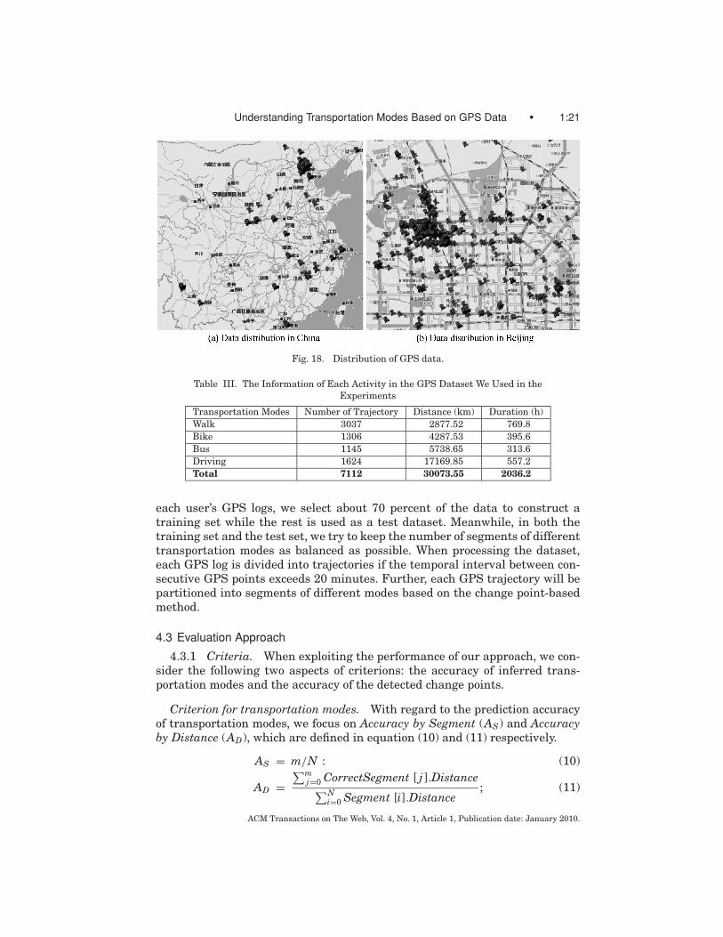
4.2.2 GPS Data. Figure 18 shows the distribution of the GPS data we usedin the experiments. Carrying a GPS-enabled device, 65 users recorded theiroutdoor movements with GPS logs over a period of 10 months. The datasetcovers 28 big cities in China and some cities in the USA, South Korea, andJapan. We pay each data collector based on the distance of GPS trajectoriesthey collected and labeled, and use this dataset anonymously.

As shown in Table III, the total distance of these GPS logs exceeds 30,000kilometers, and their total duration equates to more than 2,000 hours. From



Fig. 18. Distribution of GPS data.

Table III. The Information of Each Activity in the GPS Dataset We Used in theExperiments

Transportation Modes Number of Trajectory Distance (km) Duration (h)Walk 3037 2877.52 769.8Bike 1306 4287.53 395.6Bus 1145 5738.65 313.6Driving 1624 17169.85 557.2Total 7112 30073.55 2036.2

each user’s GPS logs, we select about 70 percent of the data to construct atraining set while the rest is used as a test dataset. Meanwhile, in both thetraining set and the test set, we try to keep the number of segments of differenttransportation modes as balanced as possible. When processing the dataset,each GPS log is divided into trajectories if the temporal interval between con-secutive GPS points exceeds 20 minutes. Further, each GPS trajectory will bepartitioned into segments of different modes based on the change point-basedmethod.

4.3 Evaluation Approach

4.3.1 Criteria. When exploiting the performance of our approach, we con-sider the following two aspects of criterions: the accuracy of inferred trans-portation modes and the accuracy of the detected change points.

Criterion for transportation modes. With regard to the prediction accuracyof transportation modes, we focus on Accuracy by Segment (AS) and Accuracyby Distance (AD), which are defined in equation (10) and (11) respectively.

AS = m/N : (10)

AD =∑m

j=0 CorrectSegment [ j ].Distance∑N

i=0 Segment [i].Distance; (11)



where N stands for the total number of the segments, while m denotes thenumber of segments being correctly predicted. Intuitively, it is more importantto correctly infer a segment with long distance than that with short distance.So, AD is more objective to measure the inference accuracy.

Criterion for change points. Regarding the inference accuracy of changepoints, we explore their recall and precision in two stages. In the first stage,after being partitioned by the change point-based segmentation method, a setof change points are detected from each trajectory. At this moment, the changepoints are vertexes of the estimated Walk-Segments. Here, we can use the cri-terion to measure the effectiveness of the segmentation method. In the secondstage, we evaluate the precision and recall of change points after the inferenceprocess. At this moment, a change point occurs if the inferred transportationmodes of consecutive segments are different.

If the distance between an inferred change point and its ground truth iswithin 150 meters, we regard the change point as a correct inference. Intrin-sically, if a change point is missed in a segmentation process, two segmentsof different transportation modes will be deemed as one segment of the samemode. Therefore, a false inference will definitely occur no matter what kind ofinference model we employed later. However, even if a trajectory containingonly one transportation mode is carelessly partitioned into several segments,we still have chances to infer these separated segments correctly. Later, thesesegments having the same inference results can be merged into one trajectory.However, in the segmentation phase, a very poor precision of change points willcause too much trivial segments with short distance. Subsequently, the shortdistance will damage the inference accuracy of transportation modes of a seg-ment. At the same time, a very low precision of change points will bring baduser experiences. Consequently, we claim that although the recall of a changepoint has relatively higher priority over the precision, we still need to keep thebalance between them.

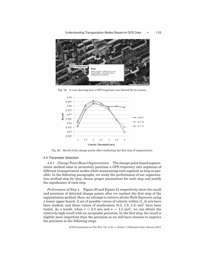
4.3.2 Ground Truth. In each day of the data collection, to help data cre-ators manually label their GPS trajectories, we respectively visualize each traceon a map for each creator. Therefore, these data-creators can view the times-tamp of each GPS point, and reflect on when and where they change transporta-tion modes. Given the short time span between data created and data labeled,we believe users are able to accurately label their GPS trajectory based on theirreliable memory and the visualized geographic clues.

Figure 19 presents a case in which a user travels on foot from 20:30:15 to20:35:56, and then transfers to driving at 20:35:58. The GPS trajectory can belabeled in a manner of “DateTime1-DateTime2 transportation mode”. In thiscase, the labeled ground truth should be

“2008-06-22 20:30:15 to 2008-06-22 20:35:56 Walk”;“2008-06-22 20:35:58 to 2008-06-22 20:55:28 Driving.”

Later, a change point is easy to be detected based on such labels.



Fig. 19. A case showing how a GPS trajectory was labeled by its creator.

0.945

0.95

0.955

0.96

0.965

0.97

0.975

0.98

0.985

0.99

1 1.5 2 2.5 3 3.5 4

Rec

all

Velocity Threshold (m/s)

a=0.2

a=1.0

a=1.5

Fig. 20. Recall of the change points after conducting the first step of segmentation.

4.4 Parameter Selection

4.4.1 Change Point-Based Segmentation. The change point-based segmen-tation method aims to accurately partition a GPS trajectory into segments ofdifferent transportation modes while maintaining each segment as long as pos-sible. In the following paragraphs, we study the performance of our segmenta-tion method step by step, choose proper parameters for each step and justifythe significance of each step.

Performance of Step 1. Figure 20 and Figure 21 respectively show the recalland precision of detected change points after we conduct the first step of thesegmentation method. Here, we attempt to retrieve all the Walk Segments usinga looser upper bound. A set of possible values of velocity within [1, 4] m/s havebeen studied, and three values of acceleration (0.2, 1.0, 1.5) m/s2 have beentested. As a result, when v = 2.5 m/s and a = 1.5 m/s2, we can obtain therelatively high recall with an acceptable precision. In the first step, the recall isslightly more important than the precision as we still have chances to improvethe precision in the following steps.



0.005

0.01

0.015

0.02

0.025

0.03

0.035

1 1.5 2 2.5 3 3.5 4

Pre

cisi

on

Velocity Threshold (m/s)

a=0.2

a=1.0

a=1.5

Fig. 21. Precision of the change points after conducting the first step of segmentation.

0.7

0.75

0.8

0.85

0.9

0.95

10 20 30 40 50 60

Rec

all

Minimal Distance Bound(m)

TS = 5s

TS = 10s

TS = 20s

TS = 30s

Fig. 22. Recall of the change points after conducting the second step of segmentation.

Performance of Step 2. After being processed by the first step of our method,a GPS trajectory is partitioned into many Walk Segments and non-Walk seg-ments. Two parameters, minimal distant bound (MDB) and minimal time span(TS) of a segment, are employed in the second step to improve the precision ofthe segmentation by merging these trivial segments. From the data depictedin Figure 22 and Figure 23, when MDB = 20 meters and TS = 10 seconds, weobtain a relatively high recall with an acceptable precision of detected changepoints. In other words, if the distance of a segment is smaller than 20 metersor the time span between its start time and end time is less than 10 seconds,this segment will be merged into its backward segments.

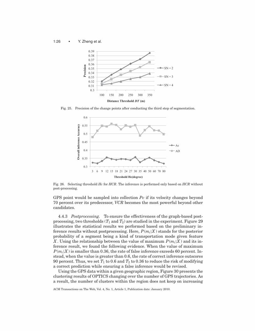
Performance of Step 3. Figure 24 and Figure 25 present the segmentationperformance of the third step of our method. In this step, if the number ofconsecutive Uncertain Segments exceeds a threshold SN, these Uncertain Seg-ments will be merged into one segment. Therefore, two parameters need to bestudied. One is the distance threshold of a Certain Segment (DT). The other isthe number of consecutive Uncertain Segments. As a result, we find that whenSN = 2 and DT = 200 meters, the segmentation method achieves an acceptable



0.1

0.15

0.2

0.25

0.3

0.35

0.4

0.45

0.5

0.55

10 20 30 40 50 60

Pre

cisi

on

Minimal Distance Bound(m)

TS = 5s

TS = 10s

TS = 20s

TS = 30s

Fig. 23. Precision of the change points after conducting the second step of segmentation.

0.85

0.86

0.87

0.88

0.89

100 150 200 250 300 350

Rec

all

Distance Threshold DT (m)

SN = 2

SN = 3

SN = 4

Fig. 24. Recall of the change points after conducting the third step of segmentation.

recall with relatively high precision. In other words, if the distance of a segmentis less than 200 meters, it is regarded as an Uncertain Segment. If the numberof consecutive Uncertain Segments exceeds two, these segments will be mergedinto one segment.

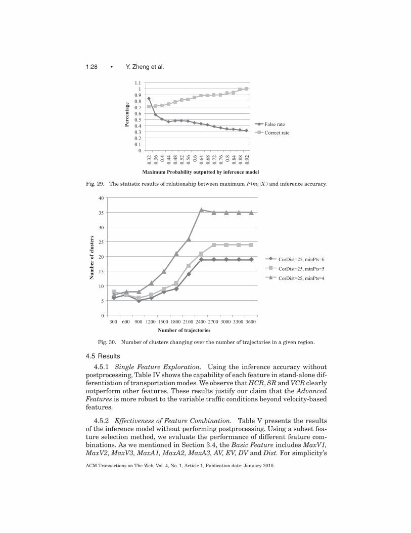
4.4.2 Advanced Features. Figure 26 shows the inference accuracy chang-ing over the threshold (Hc) when HCR is used alone to differentiate differenttransportation modes. The curve painted in Figure 26 presents us with theprior knowledge that HCR becomes the most discriminative when Hc is set to15 degrees. In other words, when a user changes his/her heading direction bya angle greater than 15 degrees, the corresponding GPS point will be sampledinto the collection Pc, and further calculate HCR according to Equation (3).

As depicted in Figure 27, we study the effect of SR in stand-alone predictingtransportation modes. Obviously, we can get the suggestion that, as comparedto other candidates, when Vs equals to 2.5, SR shows its greatest advantagesin classifying different modes.

Figure 28 depicts the inference accuracy changing over the threshold Vr whenwe employ VCR alone. We found evidence that when Vr is set to 0.7, that is, a



0.30.310.320.330.340.350.360.370.380.39

100 150 200 250 300 350

Pre

cisi

on

Distance Threshold DT (m)

SN = 2

SN = 3

SN = 4

Fig. 25. Precision of the change points after conducting the third step of segmentation.

0.3

0.35

0.4

0.45

0.5

0.55

0.6

3 6 9 12 15 18 21 24 27 30 35 40 50 60 70 80

Ove

rall

infe

renc

e A

ccur

acy

Threshold Hc(degree)

As

AD

Fig. 26. Selecting threshold Hc for HCR. The inference is performed only based on HCR withoutpost-processing.

GPS point would be sampled into collection Pv if its velocity changes beyond70 percent over its predecessor, VCR becomes the most powerful beyond othercandidates.

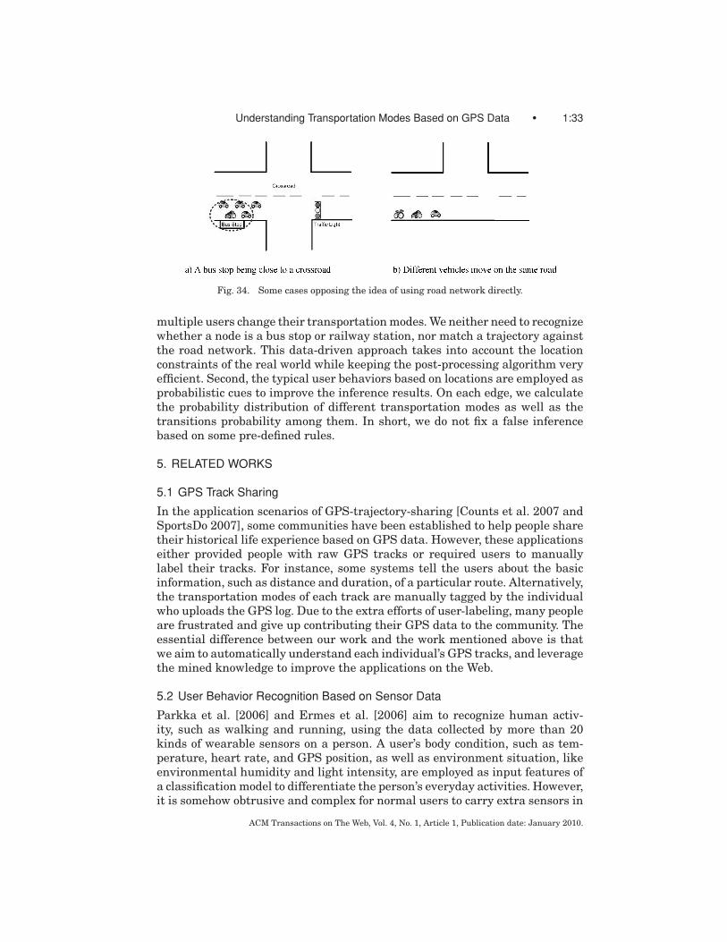
4.4.3 Postprocessing. To ensure the effectiveness of the graph-based post-processing, two thresholds (T1 and T2) are studied in the experiment. Figure 29illustrates the statistical results we performed based on the preliminary in-ference results without postprocessing. Here, P (mi|X ) stands for the posteriorprobability of a segment being a kind of transportation mode given featureX . Using the relationship between the value of maximum P (mi|X ) and its in-ference result, we found the following evidence. When the value of maximumP (mi|X ) is smaller than 0.36, the rate of false inference exceeds 60 percent. In-stead, when the value is greater than 0.6, the rate of correct inference outscores90 percent. Thus, we set T1 to 0.6 and T2 to 0.36 to reduce the risk of modifyinga correct prediction while ensuring a false inference would be revised.

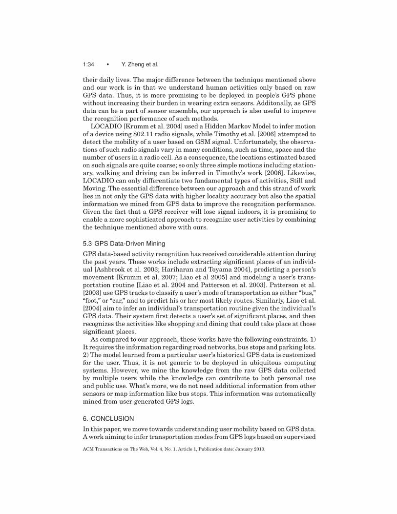
Using the GPS data within a given geographic region, Figure 30 presents theclustering results of OPTICS changing over the number of GPS trajectories. Asa result, the number of clusters within the region does not keep on increasing



0.2

0.25

0.3

0.35

0.4

0.45

0.5

0.55

0.6

0.5 1 1.5 2 2.5 3 3.5 4 4.5 5

Ove

rall

Infe

renc

e A

ccyr

acy

Threshold Vs(m/s)

As

AD

Fig. 27. Selecting threshold (Vs) for SR. SR is the only feature used in the inference model withoutpost-processing.

0.25

0.3

0.35

0.4

0.45

0.5

0.55

0.1 0.3 0.5 0.7 0.9 1.1 1.3 2 5

Ove

rall

Infe

renc

e A

ccur

acy

Threshold Vr(m/s)

As

AD

Fig. 28. Selecting threshold (Vr) for VCR. VCR is the only feature used in the inference modelwithout post-processing.

with the incrementally added GPS trajectories. It proves that the number ofplaces where most people change their transportation modes in a given region islimited, and is constrained by the real world. This observation also provides pos-itive support on the feasibility of our graph-based postprocessing. With regardto the OPTICS algorithm, its result depends on two parameters, core-distance(CorDist) and minimal points (minPts) within the core-distance. According tothe commonsense knowledge of real world and experimental evaluation, wefound that when CorDist = 25 and minPts = 5, the distribution of clustersmakes more sense than that based on other parameters.

Figure 31 paints a case of a change point-based graph on a map, and displaysthe most popular transportation mode on each graph edge. Each circle standsfor a cluster and the line between two circles represents a graph edge.



00.10.20.30.40.50.60.70.80.9

11.1

0.32

0.36 0.

40.

440.

480.

520.

56 0.6

0.64

0.68

0.72

0.76 0.

80.

840.

880.

92

Per

cent

age

Maximum Probability outputted by inference model

False rate

Correct rate

Fig. 29. The statistic results of relationship between maximum P (mi |X ) and inference accuracy.

0

5

10

15

20

25

30

35

40

300 600 900 1200 1500 1800 2100 2400 2700 3000 3300 3600

Num

ber

of c

lust

ers

Number of trajectories

CorDist=25, minPts=6



Fig. 30. Number of clusters changing over the number of trajectories in a given region.

4.5 Results

4.5.1 Single Feature Exploration. Using the inference accuracy withoutpostprocessing, Table IV shows the capability of each feature in stand-alone dif-ferentiation of transportation modes. We observe that HCR, SR and VCR clearlyoutperform other features. These results justify our claim that the AdvancedFeatures is more robust to the variable traffic conditions beyond velocity-basedfeatures.

4.5.2 Effectiveness of Feature Combination. Table V presents the resultsof the inference model without performing postprocessing. Using a subset fea-ture selection method, we evaluate the performance of different feature com-binations. As we mentioned in Section 3.4, the Basic Feature includes MaxV1,MaxV2, MaxV3, MaxA1, MaxA2, MaxA3, AV, EV, DV and Dist. For simplicity’s



Fig. 31. A change point-based graph within a region.

Table IV. Overall Inference Accuracy Using Each Feature Alone

Rank Features AS AD Rank Features AS AD

1 HCR 0.345 0.561 8 DV 0.269 0.3572 SR 0.335 0.561 9 MaxV2 0.322 0.3443 AV 0.382 0.547 10 MaxV1 0.294 0.2574 VCR 0.336 0.526 11 MaxA2 0.239 0.2175 EV 0.375 0.523 12 MaxA1 0.259 0.2086 Dist 0.302 0.499 13 MaxA3 0.256 0.1977 MaxV3 0.334 0.365

sake, the combination of the Basic Features and the Advance Features is calledFull Feature.

From the results shown in Table V, we can make two observations. First,the combination of the Advanced Features (SR+HCR+VCR) is more effectivethan that of velocity and acceleration in predicting users’ transportation modes.It justified our statement that these three features are more robust to trafficconditions than the Basic Features. Second, by combining SR+HCR+VCR withthe Basic Features, we attain the highest accuracy. This evidence further provesthat the Advanced Feature is discriminative and has little correlation betweenBasic Features. In this experiment, the inference results of Basic features areslightly less than those reported in paper [Zheng et al. 2008a] due to the in-creased test data.

4.5.3 Effectiveness of Segmentation. Using the Full Features, we evalu-ate the performance of the change point-based segmentation method. We com-pare our method with two baseline trajectory-partition approaches, including



Table V. Inference Performance of Combined Features Without PerformingPostprocessing

Transportation Mode Change PointFeature Combinations AS AD Precision RecallMaxA1 + MaxA2 + MaxA3 0.297 0.283 0.118 0.584MaxV1 + MaxV2 + MaxV3 0.480 0.526 0.142 0.687Distance + EV + AV 0.480 0.550 0.227 0.582Distance + EV + MaxV1 0.548 0.597 0.217 0.55AV + EV + MaxV1 0.558 0.621 0.253 0.603MaxV3 + MaxA3 + AV 0.511 0.632 0.138 0.669SR + HCR + VCR 0.575 0.644 0.286 0.643Basic Features 0.618 0.673 0.284 0.681Enhanced Features 0.635 0.715 0.373 0.724

0

0.1

0.2

0.3

0.4

0.5

0.6

0.7

0.8

AD AS Change Point-Recall

Change Point-Precision

Per

cent

age

Evaluation Criteria

Change Point-Based

Uniform Duration-Based (120 s)

Uniform Distance-Based (200 m)

Fig. 32. Comparison among different segmentation methods.

uniform distance-based and uniform duration-based methods. A set of param-eters have been studied for these two baseline methods. As a result, we findthat when the unit distance is set to 200 meters, the uniform distance-basedsegmentation method achieved a relatively high performance among the se-lected parameter candidates. Meanwhile, when we configure the unit durationas 120 seconds, the uniform-based method obtained a relatively high perfor-mance. Therefore, Figure 32 shows only the comparison results between ourmethod and the baseline method with the best performance. As we can see,except for the accuracy by segment (AS), the change point-based segmentationmethod outperforms its competitors in all the rest of the evaluation criteria.

4.5.4 Effectiveness of Postprocessing. Figure 33 shows the inference perfor-mance with and without post-processing. Based on the inference model usingFull Features (Advanced Features + Basic Features), the normal postprocess-ing has achieved almost 2 percent improvement in accuracy (AD) beyond thepreliminary results. Further, the graph-based postprocessing outperforms thenormal method by bringing a 4-percent promotion over the preliminary in-ferences. Additionally, the graph-based postprocessing algorithm provides a5-percent improvement to the precision of change points over the preliminaryinference results while maintaining almost the same recall of change points.



0

0.1

0.2

0.3

0.4

0.5

0.6

0.7

0.8

AS AD Precision Recall

Transportation Mode Change Point

Per

cent

age

Evaluation Criteria

Full Features (FF)

FF + Normal Post-Processing

FF + Graph-Based Post-Processing

Fig. 33. Evaluation of the post-processing algorithm.

Table VI. Confusion Matrix of Final Inference Results with Graph-BasedPostprocessing

Inferred Results (KM)Walk Driving Bus Bike

Walk 752.8 107.4 81.5 78.3 0.738Driving 41.7 2867.5 563.0 88.3 0.805

Ground Truth Bus 58.6 425.7 1489.8 105.1 0.717 RecallBike 58.9 21.8 290.0 833.1 0.692

0.825 0.837 0.615 0.754 0.756Precision

Table VI presents detailed inference results, including precision and recallof each kind of transportation mode by distance. With a large-scale dataset, webelieve that the graph-based postprocessing would bring a greater improvementto current experimental results. First, with more GPS data, the change point-based graph could cover more places where people log their trajectories withGPS data. Thus, more inferred GPS trajectories can be matched on the graph,and further be processed by the graph-based method. Second, the probabilitydistribution on the graph would become more capable of representing typicaluser behavior on locations.

4.6 Discussion

4.6.1 Discussion of the Segmentation Method. Given the data shown inFigure 32, we made the following observations. Regarding the uniform distance-based and uniform duration-based methods, they are more likely to put consecu-tive segments of different transportation modes into one segment, and generatemany trivial segments with short distances. Thus, as compared to the changepoint-based approach, it is inevitable that some change points will be missedand more false inferences will be generated. Further, these false inferences willdamage the precision of the change points and bring a very bad user experi-ence of browsing a trajectory. Although, these baseline methods also providerelatively good AS , their poor precision of change points reveal the fact that



the correct inferences and false inferences alternate in a trajectory. As a con-sequence, people are easily confused by the inference result when browsing atrajectory’s transportation mode.

The advantages of the change point-based segments lie in two aspects. Oneis that this approach is capable of maintaining a segment of one transportationmode as long as possible. Therefore, we are more likely to extract discrimina-tive features from each segment and obtain a correct inference. The other isthat its merging strategy can handle, to some extent, the vulnerability of fea-tures facing variable traffic conditions. In congestion, a user reluctantly movesfast and slow in an alternative manner. If the change point-based segmenta-tion method is employed, these segments might be merged into one segment.However, this trajectory will be partitioned into many trivial segments by theuniform distance or uniform duration-based method.

4.6.2 Discussion on the Advanced Features. The results reported inTable IV and Table V justified the effectiveness of Advanced Features in classi-fying transportation modes. Whether being used alone or in combination, theAdvanced Features always shows its advantages over the Basic Features. Itis not difficult to understand that Advanced Features extracted from a user’strajectory depends more on the characteristics of the vehicle the user selectedrather than the traffic conditions. For instance, buses and cars cannot changetheir moving direction as flexibly as people traveling on foot. This fact would notvary with traffic conditions. Therefore, the reasons why our approach is capableof tackling the affects of heavy traffic include three parts: 1) the change point-based segmentation methods; 2) the Advanced Features we identified; and 3)the graph-based post-processing method.

4.6.3 Discussion on the Graph-Based Postprocessing. The data shown inFigure 33 and Table VI has shown the contributions that the graph-basedpost-processing makes in improving the inference accuracy. Here, we mine animplied road network from user-generated GPS logs rather than directly em-ploying a database of map information. Actually, it is impractical to directlymatch a user’s trajectory against a road network and bus stops due to thefollowing reasons. First, as depicted in Figure 34(a), the locations of bus stopsare usually close to crossroads. Hence, it is really difficult to judge whether aperson was driving or taking a bus based on the observation that the user haspassed a region containing a bus stop. In other words, it is also possible that theuser might drive a car and wait a traffic light at a crossroad near the bus stop.Second, as demonstrated in Figure 34(b), bikes, buses and cars usually moveon the same road surface in an urban area. That may sometimes contradict theassumption that if an individual’s trajectory aligns with a highway, the indi-vidual might be driving at that moment. Third, matching a trajectory againsta given road network would need lots of computational efforts, which easy intheory but difficult in practice.

As opposed to the straightforward method already mentioned, we mine aninvisible graph from user-generated GPS logs. The advantages of this graphconsist of two parts. First, in this graph, each node just represents a place where



Fig. 34. Some cases opposing the idea of using road network directly.

multiple users change their transportation modes. We neither need to recognizewhether a node is a bus stop or railway station, nor match a trajectory againstthe road network. This data-driven approach takes into account the locationconstraints of the real world while keeping the post-processing algorithm veryefficient. Second, the typical user behaviors based on locations are employed asprobabilistic cues to improve the inference results. On each edge, we calculatethe probability distribution of different transportation modes as well as thetransitions probability among them. In short, we do not fix a false inferencebased on some pre-defined rules.

5. RELATED WORKS

5.1 GPS Track Sharing

In the application scenarios of GPS-trajectory-sharing [Counts et al. 2007 andSportsDo 2007], some communities have been established to help people sharetheir historical life experience based on GPS data. However, these applicationseither provided people with raw GPS tracks or required users to manuallylabel their tracks. For instance, some systems tell the users about the basicinformation, such as distance and duration, of a particular route. Alternatively,the transportation modes of each track are manually tagged by the individualwho uploads the GPS log. Due to the extra efforts of user-labeling, many peopleare frustrated and give up contributing their GPS data to the community. Theessential difference between our work and the work mentioned above is thatwe aim to automatically understand each individual’s GPS tracks, and leveragethe mined knowledge to improve the applications on the Web.

5.2 User Behavior Recognition Based on Sensor Data

Parkka et al. [2006] and Ermes et al. [2006] aim to recognize human activ-ity, such as walking and running, using the data collected by more than 20kinds of wearable sensors on a person. A user’s body condition, such as tem-perature, heart rate, and GPS position, as well as environment situation, likeenvironmental humidity and light intensity, are employed as input features ofa classification model to differentiate the person’s everyday activities. However,it is somehow obtrusive and complex for normal users to carry extra sensors in



their daily lives. The major difference between the technique mentioned aboveand our work is in that we understand human activities only based on rawGPS data. Thus, it is more promising to be deployed in people’s GPS phonewithout increasing their burden in wearing extra sensors. Additonally, as GPSdata can be a part of sensor ensemble, our approach is also useful to improvethe recognition performance of such methods.

LOCADIO [Krumm et al. 2004] used a Hidden Markov Model to infer motionof a device using 802.11 radio signals, while Timothy et al. [2006] attempted todetect the mobility of a user based on GSM signal. Unfortunately, the observa-tions of such radio signals vary in many conditions, such as time, space and thenumber of users in a radio cell. As a consequence, the locations estimated basedon such signals are quite coarse; so only three simple motions including station-ary, walking and driving can be inferred in Timothy’s work [2006]. Likewise,LOCADIO can only differentiate two fundamental types of activities, Still andMoving. The essential difference between our approach and this strand of worklies in not only the GPS data with higher locality accuracy but also the spatialinformation we mined from GPS data to improve the recognition performance.Given the fact that a GPS receiver will lose signal indoors, it is promising toenable a more sophisticated approach to recognize user activities by combiningthe technique mentioned above with ours.

5.3 GPS Data-Driven Mining

GPS data-based activity recognition has received considerable attention duringthe past years. These works include extracting significant places of an individ-ual [Ashbrook et al. 2003; Hariharan and Toyama 2004], predicting a person’smovement [Krumm et al. 2007; Liao et al 2005] and modeling a user’s trans-portation routine [Liao et al. 2004 and Patterson et al. 2003]. Patterson et al.[2003] use GPS tracks to classify a user’s mode of transportation as either “bus,”“foot,” or “car,” and to predict his or her most likely routes. Similarly, Liao et al.[2004] aim to infer an individual’s transportation routine given the individual’sGPS data. Their system first detects a user’s set of significant places, and thenrecognizes the activities like shopping and dining that could take place at thosesignificant places.

As compared to our approach, these works have the following constraints. 1)It requires the information regarding road networks, bus stops and parking lots.2) The model learned from a particular user’s historical GPS data is customizedfor the user. Thus, it is not generic to be deployed in ubiquitous computingsystems. However, we mine the knowledge from the raw GPS data collectedby multiple users while the knowledge can contribute to both personal useand public use. What’s more, we do not need additional information from othersensors or map information like bus stops. This information was automaticallymined from user-generated GPS logs.

6. CONCLUSION

In this paper, we move towards understanding user mobility based on GPS data.A work aiming to infer transportation modes from GPS logs based on supervised



learning is reported. Using our approach, four kinds of transportation modes,consisting of walking, driving, taking a bus and riding a bike, are differentiatedfrom one another. Such transportation modes can feature a user’s mobility andsupport a variety of pervasive computing systems, such as human behaviorrecognition, trajectory sharing and smart route recommendation. Using theGPS logs collected by 65 people over a period of 10 months, we evaluated ourapproach via a set of experiments and produced the following results.

First, the change point-based segmentation approach outperforms the base-line methods, including uniform distance-based and uniform duration-basedsegmentation, in inferring the transportation modes and detecting changepoints of a GPS trajectory. This method can effectively partition a trajectoryinto segments of different transportation modes, while maintaining a segmentof one mode as long as possible. Consequently, this approach is more likelyto provide a better foundation for the inference model and achieve a relativehigher inference performance.

Second, beyond the Basic Features directly using velocity and acceleration,the Advanced Features, including heading change rate, stop rate, and velocitychange rate, is more discriminative in differentiating between transportationmodes. No matter being used alone or in combination, the Advanced Featuresalways shows its advantages over the Basic Features. It is not difficult to un-derstand that the Advanced Features depends more on the characteristics ofthe vehicle a user selected rather than the traffic conditions the user experi-enced. Based on the change point-based segmentation method and DecisionTree-based inference model, we achieved an inference accuracy greater than0.71 by combining the Advanced Features with Basic Features.

Third, beyond the normal postprocessing, the graph-based post-processingalgorithm brought a 4 percent improvement over the preliminary inferenceresults. In this method, we mined an implied graph from user-generated GSPlogs. This graph contains the probabilistic cues, including the commonsenseconstraints of the real world and typical user behaviors based on locations,while keeping our method independent of additional map information.

ACKNOWLEDGMENTS

Many thanks to the volunteers who helped us collect GPS data in the pastyears. We also appreciate the input of Like Liu and Longhao Wang, who helpedus conduct some experiments in the beginning of this project.

REFERENCES

ANKERST, M., BREUNIG, M. M., KRIEGEL, H., AND SANDER, J. 1999. OPTICS: Ordering points toidentify the clustering structure. In Proceedings of the ACM SIGMOD International Conferenceon Management of Data, A. Delis, C. Faloutsos, and S. Ghandeharizadeh, Eds. ACM Press, NewYork. 49–60.

ASHBROOK, D. AND STARNER, T. 2003. Using GPS to learn significant locations and predict move-ment across multiple users. Personal Ubiquitous Comput. 7, 5, 275–286.

BREIMAN, L. 1996. Bagging Predictors. Machine Learn. 24, 123–140CHEN, G. AND KOTZ D. 2000. A survey of context-aware mobile computing research. Tech. rep.

TR2000-381, 2000, Dartmouth College Hanover, NH.



COUNTS, S. AND SMITH M. 2007. Where were we: Communities for sharing space-time trails. InProceedings of the 15th International Symposium on Advances in Geographic Information Sys-tems, Samet H., Shahabi C. and Schneider M., Eds. New York. 10–18.

ERMES, M., PARKKA, J., MANTYJARVI, J., AND KORHONEN, I. 2006. Detection of daily activities andsports with wearable sensors in controlled and uncontrolled conditions. IEEE Trans. Inform.Tech. Biomed. 12, 1, 20–26.

HARIHARAN, R. AND TOYAMA, K. 2004. Parsing and modeling location histories In Proceedings ofthe 3rd International Conference on Geographic Information Science. Springer 106–124.

KRUMM, J., AND HORVITZ, E. 2006. Predestination: Inferring destinations from partial trajectories.In Proceedings of the 8th International Conference on Ubiquitous Computing. Springer-Verlag243–260.

KRUMM, J., AND HORVITZ, E. 2004. LOCADIO: Inferring motion and location from wi-fi signalstrengths. In Proceedings of the 1st International Conference on Mobile and Ubiquitous. Comput-ing. IEEE Press, 4–13.

LIAO, L., PATTERSON, D. J., FOX, D., AND KAUTZ, H. 2005. Building personal maps from GPS data.Annals N.Y. Acad. Sci. 1093, 249–265.

LIAO, L., FOX, D., AND KAUTZ, H. 2004. Learning and Inferring Transportation Routines. In Pro-ceedings of the National Conference on Artificial Intelligence. AAAI Press, 348–353.

PATTERSON, D., LIAO, L., FOX, D., AND KAUTZ, H. 2003. Inferring high-level behavior from low-levelsensors. In Proceedings of the 8th International Conference on Ubiquitous Computing. Springer,73–89.

PARKKA, J., ERMES, M., KORPIPAA, P., MANTYJARVI, J., AND PELTOLA, J. 2006. Activity classificationusing realistic data from wearable sensors. IEEE Trans. Inform. Tech. Biomed. 10, 1, 119–128.

SAHR, K., WHITE, D., AND KIMERLING, A. J. 2003. Geodesic discrete global grid systems. Cartographyand Geog. Inform. Sci. 30, 2, 121–134

SPORTSDO. 2007. http://sportsdo.net/Activity/ActivityBlog.aspxTOYAMA, H. 2004. Project lachesis: Parsing and modeling location histories, In Proceedings of the

3rd International Conference on Geographic Information Science. Springer, 106–124.TOYAMA, K., RON, L., AND ROSEWAY, A. 2003. Geographic location tags on digital images. In Pro-

ceedings of the 11th ACM International Conference on Multimedia. Lawrence A. Rowe, HarrickM. Vin, Thomas Plagemann, Prashant J. Shenoy and John R. Smith, Eds. 156–166.

TIMOTHY, S., VARSHAVSKY, A., LAMARCA, A., CHEN, M. Y., AND CHOUDHURY, T. 2006. Mobility detectionusing everyday GSM traces. In Proceedings of the 8th International Conference on UbiquitousComputing. Springer. 212–224

WANG, L., ZHENG, Y., XIE, X., AND MA, W. Y. 2008. A flexible spatio-temporal indexing scheme forlarge-scale GPS track retrieval. In Proceedings of the 9th International Conference on MobileData Management. IEEE Press. 1–8.

ZHENG, Y., LI, Q., CHEN, Y., XIE, X., AND MA, W. Y. 2008a. Understand mobility based GPS data.In Proceedings of the 10th International Conference on Ubiquitous Computing. ACM Press, 312–321.

ZHENG, Y., LIU, L., WANG, L., AND XIE, X. 2008b. Learning transportation mode from raw GPS datafor geographic applications on the Web. In Proceedings of the 11th International Conference onWorld Wide Web. ACM Press, 247–256.

ZHENG, Y., WANG, L., ZHANG, R., XIE, X., AND MA, W. Y. 2008c. GeoLife: Managing and understand-ing your past life over maps. In Proceedings of the 9th International Conference on Mobile DataManagement. IEEE Press, 211–212.

ZHENG, Y., XIE, X., AND MA, W. Y. 2008d. Search your life over maps. In Proceedings of the Inter-national Workshop on Mobile Information Retrieval. 24–27.

Received August 2008; revised February 2009; accepted August 2009


Documents

Understanding Transportation Modes Based on GPS Data … · Understanding Transportation Modes Based on GPS Data ... it is generic to be deployed in a broad range of Web applications