Understanding the characteristics of mass spectrometry

data through the use of simulation

Kevin R. Coombes1∗, John M. Koomen2, Keith A. Baggerly1, Jeffrey

S. Morris1, and Ryuji Kobayashi2

Departments of 1Biostatistics and Applied Mathematics and 2Molecular Pathol-

ogy, University of Texas M.D. Anderson Cancer Center, Houston TX 77030 USA

∗ To whom correspondence should be addressed:

Kevin R. Coombes

Department of Biostatistics and Applied Mathematics

UT M.D. Anderson Cancer Center

1515 Holcombe Blvd., Box 447

Houston TX 77030

Phone: 713-794-4154

Email: kcoombes@mdanderson.org

Keywords: mass spectrometry, MALDI, SELDI, simulation, peak capacity, peak quantifi-

cation, mass resolution, isotope distribution.

Running head: Simulating mass spectra

1

Abstract

Background: Mass spectrometry is actively being used to discover disease-related pro-

teomic patterns in complex mixtures of proteins derived from tissue samples or from easily

obtained biological fluids. The potential importance of these clinical applications has made

the development of better methods for processing and analyzing the data an active area of

research. It is, however, difficult to determine which methods are better without knowing

the true biochemical composition of the samples used in the experiments.

Methods: We developed a mathematical model based on the physics of a simple

MALDI-TOF mass spectrometer with time-lag focusing. Using this model, we implemented

a statistical simulation of mass spectra. We used the simulation to explore some of the basic

operating characteristics of MALDI or SELDI instruments.

Results: The simulation reproduced several characteristics of actual instruments. We

found that the relative mass error is affected by the time discretization of the detector (about

0.01%) and the spread of initial velocities (about 0.1%). The accuracy of calibration based

on external standards decays rapidly outide the range spanned by the calibrants. Natu-

ral isotope distributions play a major role in broadening peaks associated with individual

proteins. The area of a peak is a more accurate measure of its size than the height.

Conclusions: The model described here is capable of simulating realistic mass spectra.

The simulation should become a useful tool for generating spectra where the true inputs are

known, allowing researchers to evaluate the performance of new methods for processing and

analyzing mass spectra.

Availability: http://bioinformatics.mdanderson.org/cromwell.html

2

Introduction

Mass spectrometry is actively being used to discover disease-related proteomic patterns

in complex mixtures of proteins derived from tissue samples or from easily obtained biological

fluids such as serum, urine, or nipple aspirate fluid [Paweletz et al., 2000; Paweletz et al.,

2001; Wellmann et al., 2002; Petricoin et al., 2002; Adam et al., 2002; Adam et al., 2003;

Zhukov et al., 2003; Schaub et al., 2004]. These proteomic patterns can potentially be

used for early diagnosis, to predict prognosis, to monitor disease progression or response

to treatment, or even to identify which patients are most likely to benefit from particular

treatments.

A typical data set arising in a clinical application of mass spectrometry contains tens

or hundreds of spectra; each spectrum contains tens of thousands of intensity measurements

representing an unknown number of protein peaks. Any attempt to make sense of this

volume of data requires extensive low-level processing in order to identify the locations of

peaks and to quantify their sizes accurately. Inadequate or incorrect preprocessing methods,

however, can result in data sets that exhibit substantial biases and make it difficult to reach

meaningful biological conclusions [Baggerly et al., 2003; Sorace and Zhan, 2003; Baggerly et

al., 2004]. The low-level processing of mass spectra involves a number of complicated steps

that interact in complex ways. Typical processing steps are as follows.

(1) Calibration maps the observed time of flight to the inferred mass-to-charge ratio.

(2) Filtering removes random noise, typically electronic or chemical in origin.

(3) Baseline subtraction removes systematic artifacts, usually attributed to clusters of

ionized matrix molecules hitting the detector during early portions of the experiment,

or to detector overload.

(4) Normalization corrects for systematic differences in the total amount of protein des-

orbed and ionized from the sample plate.

3

(5) Peak detection and quantification is the primary goal of low-level processing; it

typically involves an assessment of the signal-to-noise ratio and may involve hieghts or

areas.

(6) Peak matching across samples is required because neither calibration nor peak de-

tection is perfect. Thus, the analyst must decide which peaks in different samples

correspond to the same biological molecule.

The potential importance of the clinical applications of mass spectrometry has drawn the

attention of increasing numbers of analysts. As a result, the development of better methods

for processing and analyzing the data has become an active area of research [Baggerly et

al., 2003; Coombes et al., 2003; Coombes et al., 2004; Hawkins et al., 2003; Lee et al., 2003;

Liggett et al., 2003; Rai et al., 2002; Wagner et al., 2003; Yasui, Pepe, et al., 2003; Yasui,

McLerran et al., 2003; Zhu et al., 2003]. It is, however, difficult to determine which methods

are better without knowing the true biochemical composition of the samples used in the

experiments. To deal with this problem, we have developed a simulation engine in S-Plus

(Insightful Corp., Seattle, WA) that allows us to simulate mass spectra from instruments with

different properties. In this article, we first derive the mathematical model of a physical mass

spectrometry instrument that underlies our simulation. Next, we use the model to explore

some of the low-level characteristics of mass spectrometry data, including the limits on mass

resolution and mass calibration, the role of isotope distributions, and the implications for

methods of normalization and quantification.

4

1: A physical model of a MALDI-TOF instrument

The mass spectrometry instruments most commonly applied to clinical and biological prob-

lems use a matrix-assisted laser desorption and ionization (MALDI) ion source and a time-of-

flight (TOF) detection system. Briefly, to run an experiment on a MALDI-TOF instrument,

the biological sample is first mixed with an energy absorbing matrix (EAM) such as sinap-

inic acid or α-cyano-4-hydroxycinnamic acid. This mixture is crystallized onto a metal plate.

(The commonly used method of surface enhanced laser desorption and ionization (SELDI) is

a variant of MALDI that incorporates additional chemistry on the surface of the metal plate

to bind specific classes of proteins [Merchant and Weinberger, 2000; Tang et al., 2004].) The

plate is inserted into a vacuum chamber, and the matrix crystals are struck with light pulses

from a nitrogen laser. The matrix molecules absorb energy from the laser, transfer it to the

proteins causing them to desorb and ionize, and produce a plume of ions in the gas phase.

Next, an electric field is applied, which accelerates the ions into a flight tube where they drift

until they strike a detector that records the time of flight. A quadratic transformation is used

to compute the mass-to-charge ratio (m/z) of the protein from the observed flight time. The

spectral data that results from this experiment consists of the sequentially recorded numbers

of ions arriving at the detector (the intensity) coupled with the corresponding m/z values.

Peaks in the intensity plot represent the proteins or polypeptide fragments that are present

in the sample.

We developed code to simulate experiments based on a physical model of a linear MALDI-

TOF instrument with time-lag focusing or delayed extraction [Wiley and McLaren, 1955;

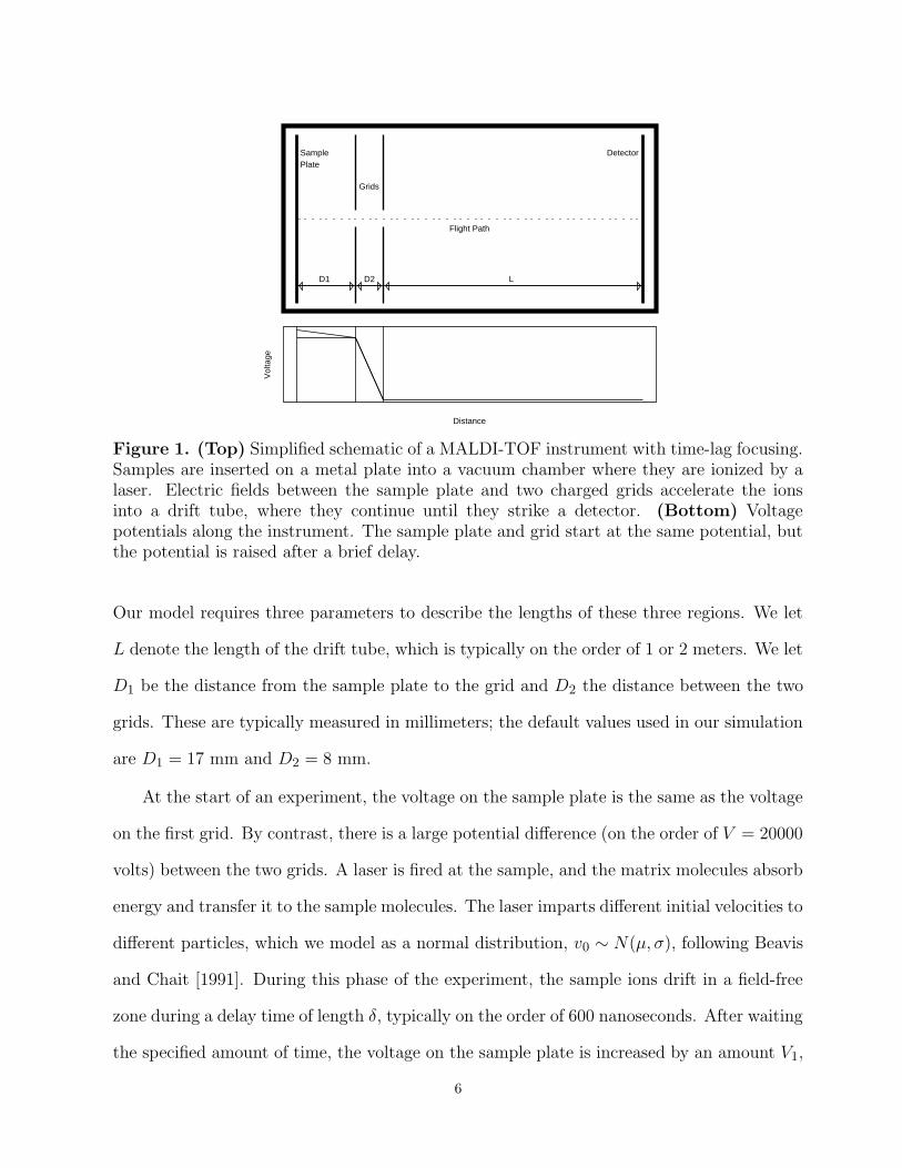
Vestal et al., 1995]. Such an instrument is illustrated schematically in Figure 1. The flight

path of a particle in this instrument passes through three regions:

(1) focusing, from the sample plate to the first grid,

(2) acceleration, through the electric field between the two charged grids, and

(3) drift, through the field-free tube from the second grid to the detector.

5

Vol

tage

050

0015

000

Vol

tage

050

0015

000

Vol

tage

050

0015

000

Vol

tage

050

0015

000

Vol

tage

050

0015

000

Vol

tage

050

0015

000

SampleSampleSample

Plate

SamplePlateSamplePlateSamplePlate

Grids

SamplePlate

Grids

Detector

Vol

tage

050

0015

000

SamplePlate

Grids

DetectorSamplePlate

Grids

Detector

Flight Path

SamplePlate

Grids

Detector

Flight Path

SamplePlate

Grids

Detector

Flight Path

SamplePlate

Grids

Detector

Flight Path

SamplePlate

Grids

Detector

Flight Path

D1

SamplePlate

Grids

Detector

Flight Path

D1 D2

SamplePlate

Grids

Detector

Flight Path

D1 D2 D2

Vol

tage

050

0015

000

SamplePlate

Grids

Detector

Flight Path

D1 D2 L

Vol

tage

SamplePlate

Grids

Detector

Flight Path

D1 D2 L

Distance

Vol

tage

Figure 1. (Top) Simplified schematic of a MALDI-TOF instrument with time-lag focusing.Samples are inserted on a metal plate into a vacuum chamber where they are ionized by alaser. Electric fields between the sample plate and two charged grids accelerate the ionsinto a drift tube, where they continue until they strike a detector. (Bottom) Voltagepotentials along the instrument. The sample plate and grid start at the same potential, butthe potential is raised after a brief delay.

Our model requires three parameters to describe the lengths of these three regions. We let

L denote the length of the drift tube, which is typically on the order of 1 or 2 meters. We let

D1 be the distance from the sample plate to the grid and D2 the distance between the two

grids. These are typically measured in millimeters; the default values used in our simulation

are D1 = 17 mm and D2 = 8 mm.

At the start of an experiment, the voltage on the sample plate is the same as the voltage

on the first grid. By contrast, there is a large potential difference (on the order of V = 20000

volts) between the two grids. A laser is fired at the sample, and the matrix molecules absorb

energy and transfer it to the sample molecules. The laser imparts different initial velocities to

different particles, which we model as a normal distribution, v0 ∼ N(µ, σ), following Beavis

and Chait [1991]. During this phase of the experiment, the sample ions drift in a field-free

zone during a delay time of length δ, typically on the order of 600 nanoseconds. After waiting

the specified amount of time, the voltage on the sample plate is increased by an amount V1,

6

typically on the order of 10% of the voltage potential between the charged grids. Different

combinations of laser power, delay time, and voltage allow the user to focus the optimum

resolution of the instrument for different mass ranges. The electric field resulting from

the voltage change causes the positively charged ions to accelerate into the region between

the charged grids, where the larger potential difference imparts a larger acceleration. The

particles then pass into the drift tube, where they continue to fly until they hit the detector.

In our model, the detector counts particles continuously (and perfectly), but it reports the

counts at discrete time intervals, with an acquisition time resolution τ on the order of a few

nanoseconds.

From the description so far, we see that a model of a linear MALDI-TOF instrument

with time-lag focusing depends on nine parameters: L, D1, D2, V , V1, δ, τ , µ, and σ.

In a real instrument, the three distance parameters are unchanging characteristics of the

design. The user has direct control over the voltages, the delay time, and the acquisition

time resolution. The parameters that determine the normal distribution of initial velocities

are controlled indirectly by the choice of EAM and by the laser intensity. Since we do not

have a good theoretical understanding of how these factors interact to determine the initial

velocity distribution, our simulation skips directly to the distribution. By default, we take

µ = 350 m/sec and σ = 50 m/sec, which are compatible with published experimental results

[Beavis and Chait, 1991; Juhasz et al., 1997].

We can compute the total time for a particle to travel from the sample plate to the

detector as a sum of four contributions: the delay time δ, the focus time tf , the acceleration

time ta, and the drift time td, which are calculated below. We assume that all particles start

the experiment attached to the sample plate (at x = 0) and that the clock starts when the

laser is fired. Each particle acquires an initial velocity v0 ∼ N(µ, σ), which is assumed to

be independent of the mass. After a delay of length δ, the particles are located at position

x0 = δv0, still traveling at velocity v0. Using the default value of δ = 600 ns and an estimated

upper bound on the velocity of 500 m/sec, the particles should be roughly 0.3 mm away from

the plate at the end of the delay period.

7

We let v1 denote the velocity of a particle at the end of the focus phase, when the

particle reaches the first grid, and we let v2 denote the velocity at the end of the acceleration

phase, when the particle reaches the second grid and enters the drift tube. It is easiest to

understand the final portion of the experiment, during which the particle travels at constant

velocity v2 through a tube of length L. So, we have

(1.1) L = v2td.

During the main acceleration phase, an electric field of voltage V accelerates a particle

of mass m with charge z through a distance D2 by applying a constant force F . Because

the work W done by the electric field is equal to the change in kinetic energy, we have

(1.2) W = zV = FD2 =mv2

2

2−

mv21

2.

Solving equation 1.1 for the velocity and substituting, we find that

(1.3) zV =m

2

(

L2

t2d− v2

1

)

.

So,

(1.4) t2d =L2

2zV/m+ v21

.

During the simulation, everything in this equation is known except for the drift time td and

the velocity v1 that marks the transition from the focusing phase of the experiment to the

acceleration phase.

During the focusing phase, the electric field generated by the potential difference V1

applies a constant force F to the particle. We can determine the force from the work

that would be done moving a particle from the sample plate to the first grid, which yields

FD1 = zV1. During this phase, however, the particle is acclerated through a distance

D1− x0, resulting in change of velocity from v0 to v1. Using the equality between work and

the change in kinetic energy, we find

(1.5)mv2

1

2−

mv20

2= F (D1 − x0) =

zV1

D1(D1 − x0).

8

Solving for the velocity v1, we find

(1.6) v21 = v2

0 +2zV1

mD1(D1 − x0).

Since all the quantities on the right hand side of this equation are assumed to be known, we

can combine it with equation (1.4) to compute the drift time as

(1.7) t2d = L2/

(

2zV

m+

2zV1

m

D1 − x0

D1+ v2

0

)

.

We now turn our attention to the time spent in the acceleration and focusing phases

of the experiment. During both phases, the particle is subject to a constant force, and

so undergoes constant acceleration. In these circumstances, one knows that the change in

velocity is equal to the acceleration times the duration. As we have seen, the force during

the main acceleration phase is F = zV/D2. Combining this with Newton’s Second Law, we

have a = zV/mD2, so

(1.8) ta =v2 − v1

a=

mD2

zV(v2 − v1) =

mD2

zV

(

L

td− v1

)

.

Since td can be computed from known values using equation (1.7) and v1 can be computed

using equation (1.6), this allows us to compute the time spent during the accleration phase.

As we have also seen, the force during the focusing phase is F = zV1/D1, so the accel-

eration is a = zV1/mD1. Thus,

(1.9) tf =v1 − v0

a=

mD1

zV1(v1 − v0).

In summary, to simulate the flight time of a particle of mass m and charge z, given

the nine parameters describing the setup of the instrument during the experiment, we first

sample the initial velocity v0 from the appropriate distribution. We then compute the

position x0 = δv0 at the end of the delay phase. Next, we use (1.6) to compute v1, (1.7) to

compute the drift time, (1.8) to compute the accleration time, (1.9) to compute the focus

time, and report the total time of flight as

(1.10) TOF = δ + tf + ta + td.

9

2: Results

We now apply the model described in the previous section, and its S-Plus implementation, to

understand some of the fundamental characteristics of mass spectra. In particular, we look

at some physical factors that affect the mass resolution [Ingendoh et al., 1994; Barbacci et

al., 1997, Vestal and Juhasz, 1998], at limits on the accuracy of mass calibration [Christian

et al., 2000; Hack and Benner, 2002], at the role of isotope distributions [Zhang et al., 1997],

and at implications for the normalization and quantification of MALDI-TOF data.

2.1: Mass Resolution

Our model contains two factors that affect the mass resolution of the instrument: the acqui-

sition time resolution (or period) of the detector and the distribution of initial velocities. We

begin by considering the effect on mass resolution caused by the discretization of time by

the detector. As we will see, this effect is, in general, far smaller than that due to the spread

in initial velocities. If there were no variability in the initial velocities, then all ions with

the same mass and charge would strike the detector at the same instant. In this idealized

setting, our ability to distinguish ions of different mass would be completely determined by

the period of the detector. We can get a rough estimate of the magnitude of this effect as

follows. First, assume that v0 = 0 and that the dominant component of the time is spent in

the drift tube. Then (1.7) simplifies to

(2.1) t2d = L2/

(

2zV

m+

2zV1

m

)

=mL2

2z(V + V1).

Solving for the mass-to-charge ratio M = m/z, we obtain

(2.2) M =m

z= t2d

2(V + V1)

L2.

Differentiating with respect to time, we find that

(2.3) ∆M ≈ 4td∆tdV + V1

L2.

10

Mass/charge

Rel

ativ

e m

ass

erro

r

0 5000 10000 15000 20000

0.0

0.00

050.

0010

0.00

150.

0020

0.5 ns1 ns2 ns4 ns10 ns20 ns

Mass/charge

Abs

olut

e m

ass

erro

r

0 5000 10000 15000 20000

02

46

810

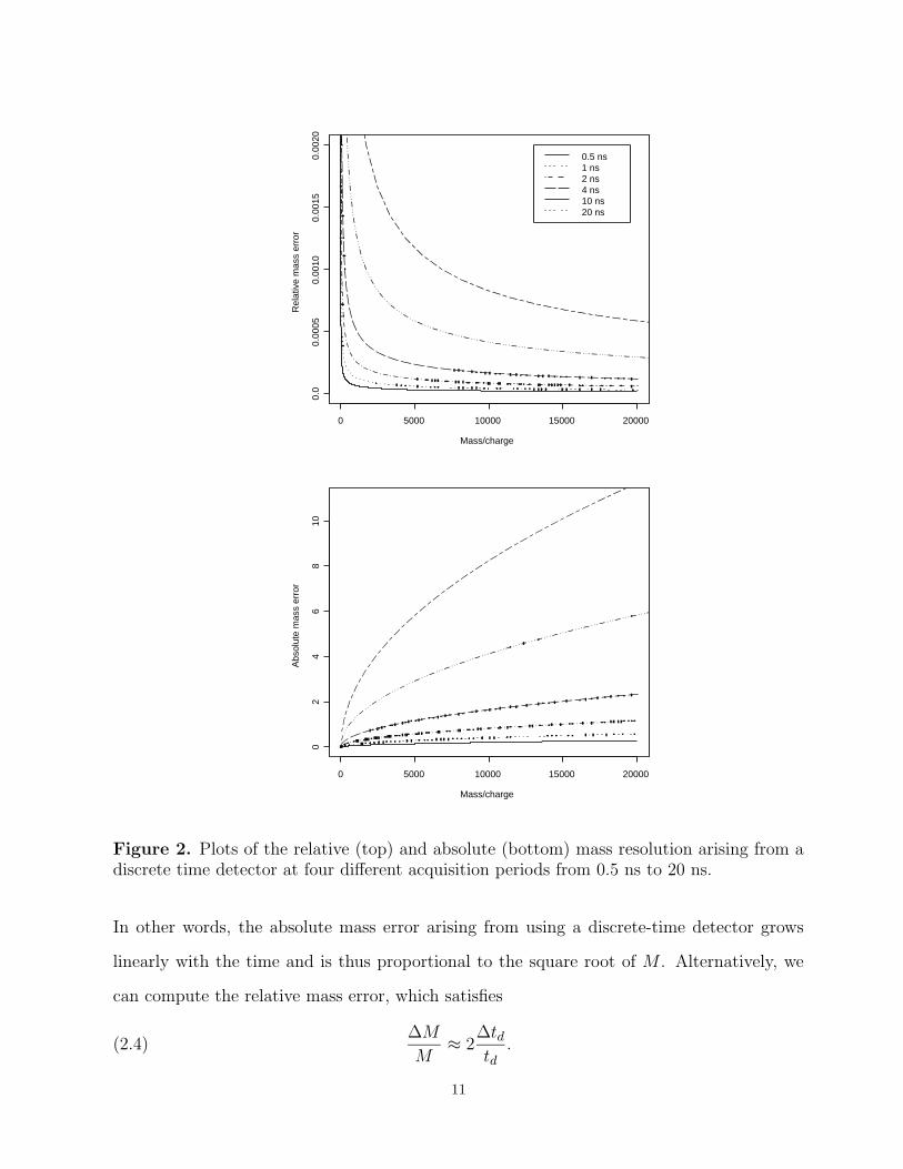
Figure 2. Plots of the relative (top) and absolute (bottom) mass resolution arising from adiscrete time detector at four different acquisition periods from 0.5 ns to 20 ns.

In other words, the absolute mass error arising from using a discrete-time detector grows

linearly with the time and is thus proportional to the square root of M . Alternatively, we

can compute the relative mass error, which satisfies

(2.4)∆M

M≈ 2

∆tdtd

.

11

So, the relative mass error is inversely proportional to the time (or to the square root of M).

12321 12357 12393 m/z

0

50

100 12360.47 R = 985

12321 12357 12393 0

50

100

MA

LD

I Io

n Si

gnal

(%

)

12360.12 R = 735

12321 12357 12393 0

50

100 12360.14 R = 1125 A

B

C

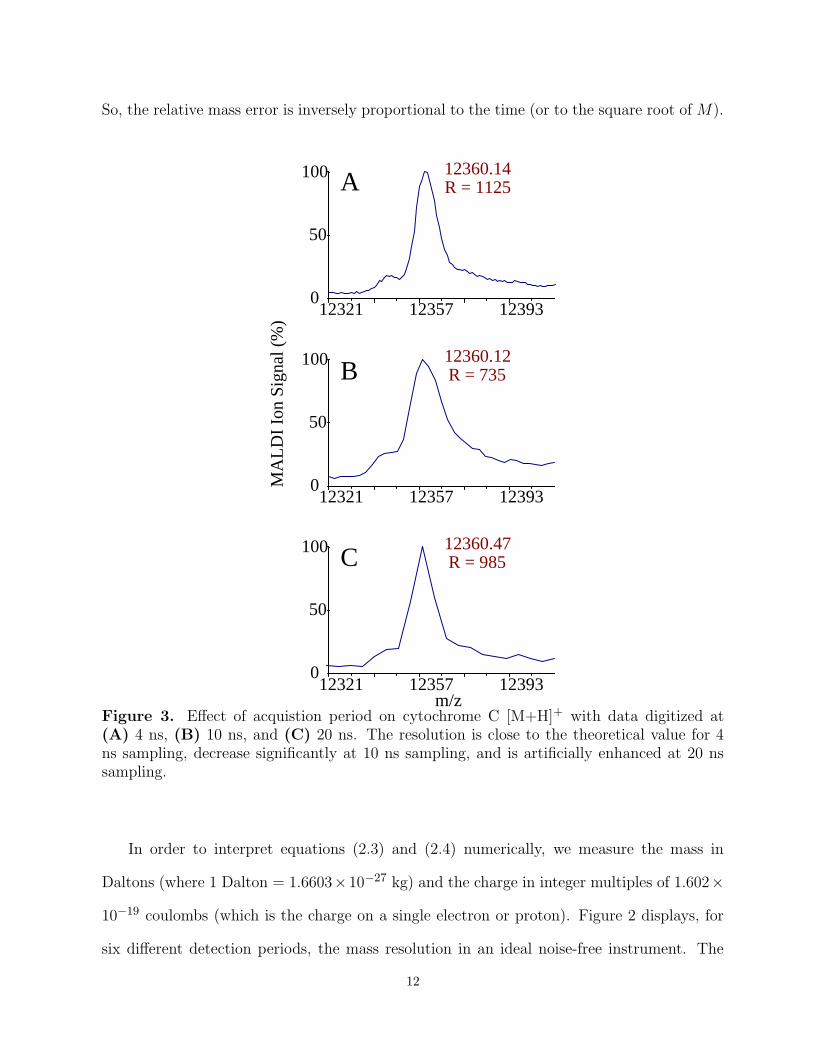
Figure 3. Effect of acquistion period on cytochrome C [M+H]+ with data digitized at(A) 4 ns, (B) 10 ns, and (C) 20 ns. The resolution is close to the theoretical value for 4ns sampling, decrease significantly at 10 ns sampling, and is artificially enhanced at 20 nssampling.

In order to interpret equations (2.3) and (2.4) numerically, we measure the mass in

Daltons (where 1 Dalton = 1.6603×10−27 kg) and the charge in integer multiples of 1.602×

10−19 coulombs (which is the charge on a single electron or proton). Figure 2 displays, for

six different detection periods, the mass resolution in an ideal noise-free instrument. The

12

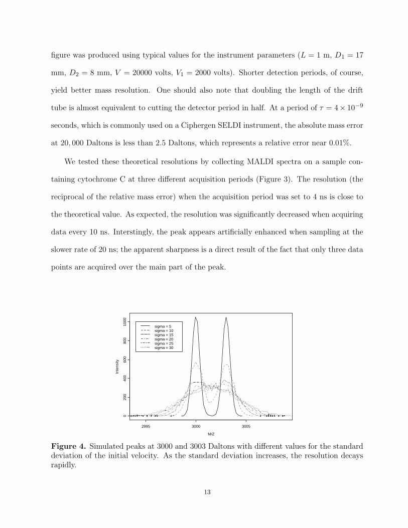
figure was produced using typical values for the instrument parameters (L = 1 m, D1 = 17

mm, D2 = 8 mm, V = 20000 volts, V1 = 2000 volts). Shorter detection periods, of course,

yield better mass resolution. One should also note that doubling the length of the drift

tube is almost equivalent to cutting the detector period in half. At a period of τ = 4× 10−9

seconds, which is commonly used on a Ciphergen SELDI instrument, the absolute mass error

at 20, 000 Daltons is less than 2.5 Daltons, which represents a relative error near 0.01%.

We tested these theoretical resolutions by collecting MALDI spectra on a sample con-

taining cytochrome C at three different acquisition periods (Figure 3). The resolution (the

reciprocal of the relative mass error) when the acquisition period was set to 4 ns is close to

the theoretical value. As expected, the resolution was significantly decreased when acquiring

data every 10 ns. Interstingly, the peak appears artificially enhanced when sampling at the

slower rate of 20 ns; the apparent sharpness is a direct result of the fact that only three data

points are acquired over the main part of the peak.

M/Z

Inte

nsity

2995 3000 3005

020

040

060

080

010

00

sigma = 5sigma = 10sigma = 15sigma = 20sigma = 25sigma = 30

Figure 4. Simulated peaks at 3000 and 3003 Daltons with different values for the standarddeviation of the initial velocity. As the standard deviation increases, the resolution decaysrapidly.

13

The relative mass error of actual MALDI-TOF instruments is typically reported in the

range of 0.1%, which suggests that factors other than the period of the detector play a larger

role. In our model, the most important factor affecting the mass resolution is the distribution

of initial velocities; this is the only stochastic factor included in the model. Figure 4 shows

the simulated spectra from ions of 3000 and 3003 Daltons, with a mean initial velocity of

350 meters/second as the standard deviation increases from 5 to 30. The twin peaks are

easily resolved when the standard deviation is small, but they gradually coalesce into a single

broad peak as the standard deviation increases.

2.2: Calibration

Calibration of a MALDI-TOF instrument is performed in order to accurately map the ob-

served time-of-flight to a mass-to-charge ratio. Calibration involves both experimental obser-

vations and theoretical computations. Most MALDI-TOF spectra are calibrated externally

by running a separate experiment, under the same conditions, using a sample that only

contains a small number (typically 5 to 7) of proteins of known mass. Computationally, we

simplify the equations of Section 1 by concentrating on the portion of the flight time spent

in the drift tube. In this way, we see that m/z is approximated by a quadratic function of

the observed flight time. The unknown coefficients of this quadratic are estimated from the

calibration spectrum using least squares.

Even under ideal conditions, the errors in this approximation can become fairly large

when the calibration equation is extrapolated beyond the range of masses of the calibrants.

We simulated calibration spectra using the default parameters from the previous section for

two different calibrant mixes. The first mix contained proteins with masses of 4, 7, 10, 12,

and 15 kDa; the second mix contained calibrants with masses of 2, 7, 12, 20, and 35 kDa.

We then simulated spectra containing masses from 1 to 50 kDa at 1000 Dalton intervals and

determined the observed “calibrated” masses from each of the two mixes. In both cases,

the mass of the 1000 Dalton protein was miscalibrated by more than 2%. Calibration errors

14

Mass/Charge

Cal

ibra

tion

Err

or

0 10000 20000 30000 40000 50000

0.0

0.00

20.

004

Mass/Charge

Cal

ibra

tion

Err

or

0 10000 20000 30000 40000 50000

0.0

0.00

20.

004

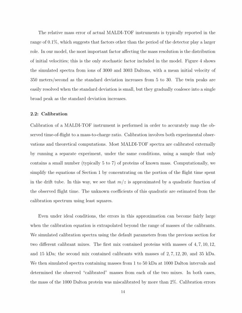
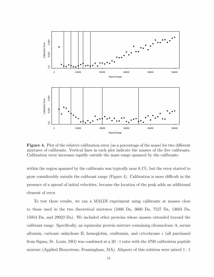
Figure 4. Plot of the relative calibration error (as a percentage of the mass) for two differentmixtures of calibrants. Vertical lines in each plot indicate the masses of the five calibrants.Calibration error increases rapidly outside the mass range spanned by the calibrants.

within the region spanned by the calibrants was typically near 0.1%, but the error started to

grow considerably outside the calibrant range (Figure 4). Calibration is more difficult in the

presence of a spread of initial velocities, because the location of the peak adds an additional

element of error.

To test these results, we ran a MALDI experiment using calibrants at masses close

to those used in the two theoretical mixtures (2466 Da, 3660 Da, 7527 Da, 13683 Da,

15054 Da, and 29023 Da). We included other proteins whose masses extended beyond the

calibrant range. Specifically, an equimolar protein mixture containing ribonuclease A, serum

albumin, carbonic anhydrase II, hemoglobin, ovalbumin, and cytochrome c (all purchased

from Sigma, St. Louis, MO) was combined at a 20 : 1 ratio with the 4700 calibration peptide

mixture (Applied Biosystems, Framingham, MA). Aliquots of this solution were mixed 1 : 1

15

with sinapinic acid (20 mg/ml) in 50% acetonitrile and 50% aqueous 0.1% TFA. Positive

ion MALDI mass spectra consisting of 250 laser shots were acquired in linear mode on an

Applied Biosystems Voyager DE-STR. Both myoglobin (m/z 16952) and serum albumin

(m/z 66431) were used as standards to optimize the resolution for small proteins and large

proteins, respectively. Typical instrument settings for the myoglobin method were 25 kV

accelerating voltage, 93% grid voltage, and 700 ns delay; for serum albumin, 25 kV, 91%,

and 900 ns were used. Resolution values were calculated by full-width at half maximum

(FWHM) using the Data Explorer software which came with the instrument. Four point

calibrations were performed using Data Explorer as well, using different peaks. The results

are shown in Table 1.

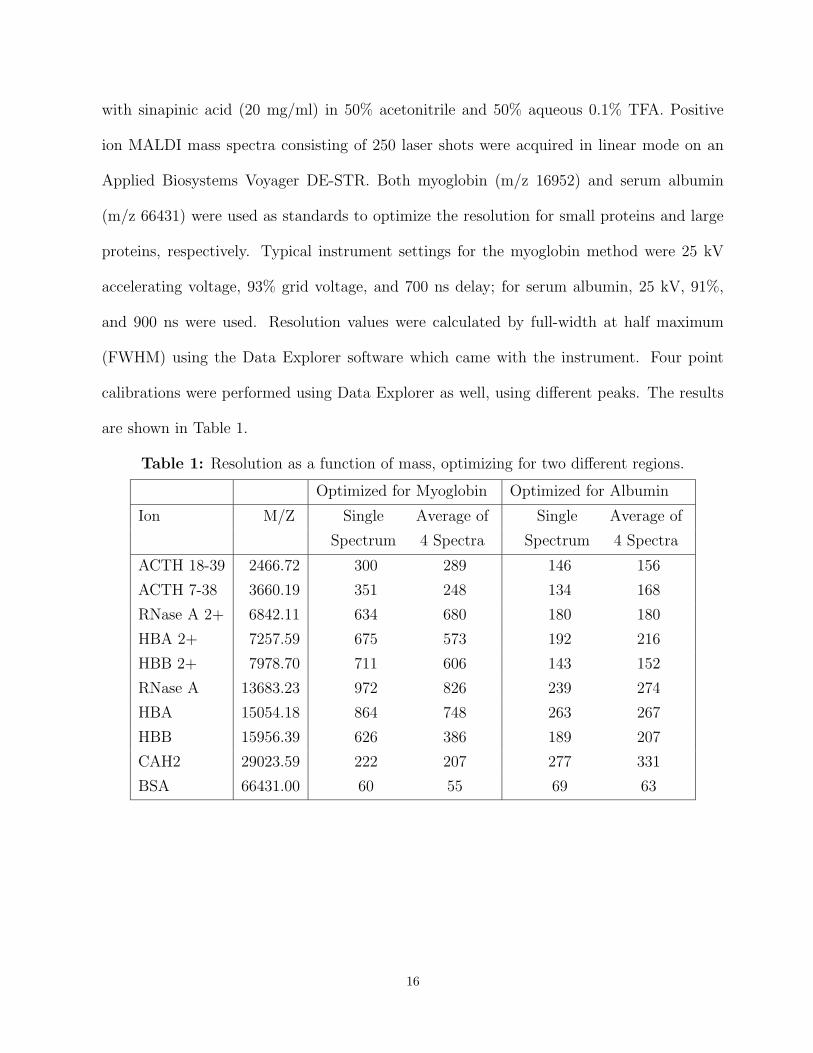
Table 1: Resolution as a function of mass, optimizing for two different regions.

Optimized for Myoglobin Optimized for Albumin

Ion M/Z Single Average of Single Average of

Spectrum 4 Spectra Spectrum 4 Spectra

ACTH 18-39 2466.72 300 289 146 156

ACTH 7-38 3660.19 351 248 134 168

RNase A 2+ 6842.11 634 680 180 180

HBA 2+ 7257.59 675 573 192 216

HBB 2+ 7978.70 711 606 143 152

RNase A 13683.23 972 826 239 274

HBA 15054.18 864 748 263 267

HBB 15956.39 626 386 189 207

CAH2 29023.59 222 207 277 331

BSA 66431.00 60 55 69 63

16

2.3: Isotope distributions

We have seen that sharply defined peaks erode quickly into broad hills as the standard

deviation of the initial velocity distribution increases. Even with fairly small values for the

standard deviation, it can be difficult to resolve peaks whose mass differs by a single Dalton.

In practice, however, even a pure solution of a single protein includes molecules whose mass

differs by one Dalton. The reason, of course, is the existence of naturally occuring stable

isotopes of common elements [Zhang et al., 1997]. Only 98.89% of naturally occuring carbon

atoms are in the form of 12C; most of the remaining 1.11% consists of atoms of 13C. In

the same way, 14N accounts for 99.63% of naturally occuring nitrogren, with the remaining

atoms in the form of 15N. Oxygen exists in three stable isotopes, with 16O accounting for

99.76% of atoms, 18O for 0.20%, and 17O for 0.04%. These three elements account for most

of the isotope differences between protein molecules (with the possible addition of a few

sulfur molecules).

Our simulation includes the isotope distributions of individual proteins. By assuming

that most of the mass of a protein is accounted for by the atoms of carbon, nitrogen, and

oxygen (with their numbers in proportions of about 6 : 2.5 : 1), we can get a crude approxi-

mation of the number of atoms that might occur as heavier isotopes by dividing the nominal

mass by 15. We then model the process of incorporating heavier isotopes using a binomial

distribution with a success rate of 0.0111. We make another simplification by assuming that

a heavier isotope always adds one to the mass (which downweights the less abundant oxygen

atoms).

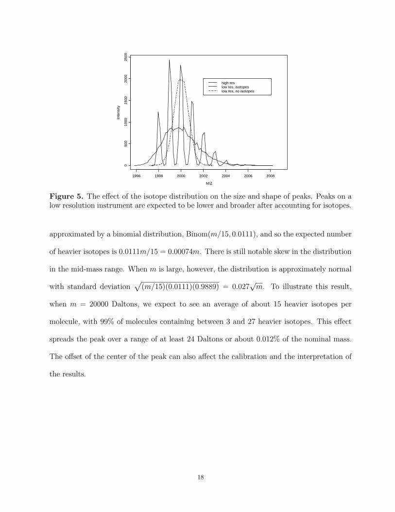
Figure 5 illustrates how accounting for the isotope distribution of a peak at 2000 Daltons

lowers and broadens the peak shape. This effect becomes more pronounced at higher masses

because there are more chances for a larger molecule to incorporate different isotopes. We

can estimate the magnitude of the effect using the same simplifications we have incorporated

in our model. The distribution of the number of heavier isotopes in a protein of mass m is

17

M/Z

Inte

nsity

1996 1998 2000 2002 2004 2006 2008

050

010

0015

0020

0025

00

high reslow res, isotopeslow res, no isotopes

Figure 5. The effect of the isotope distribution on the size and shape of peaks. Peaks on alow resolution instrument are expected to be lower and broader after accounting for isotopes.

approximated by a binomial distribution, Binom(m/15, 0.0111), and so the expected number

of heavier isotopes is 0.0111m/15 = 0.00074m. There is still notable skew in the distribution

in the mid-mass range. When m is large, however, the distribution is approximately normal

with standard deviation√

(m/15)(0.0111)(0.9889) = 0.027√m. To illustrate this result,

when m = 20000 Daltons, we expect to see an average of about 15 heavier isotopes per

molecule, with 99% of molecules containing between 3 and 27 heavier isotopes. This effect

spreads the peak over a range of at least 24 Daltons or about 0.012% of the nominal mass.

The offset of the center of the peak can also affect the calibration and the interpretation of

the results.

18

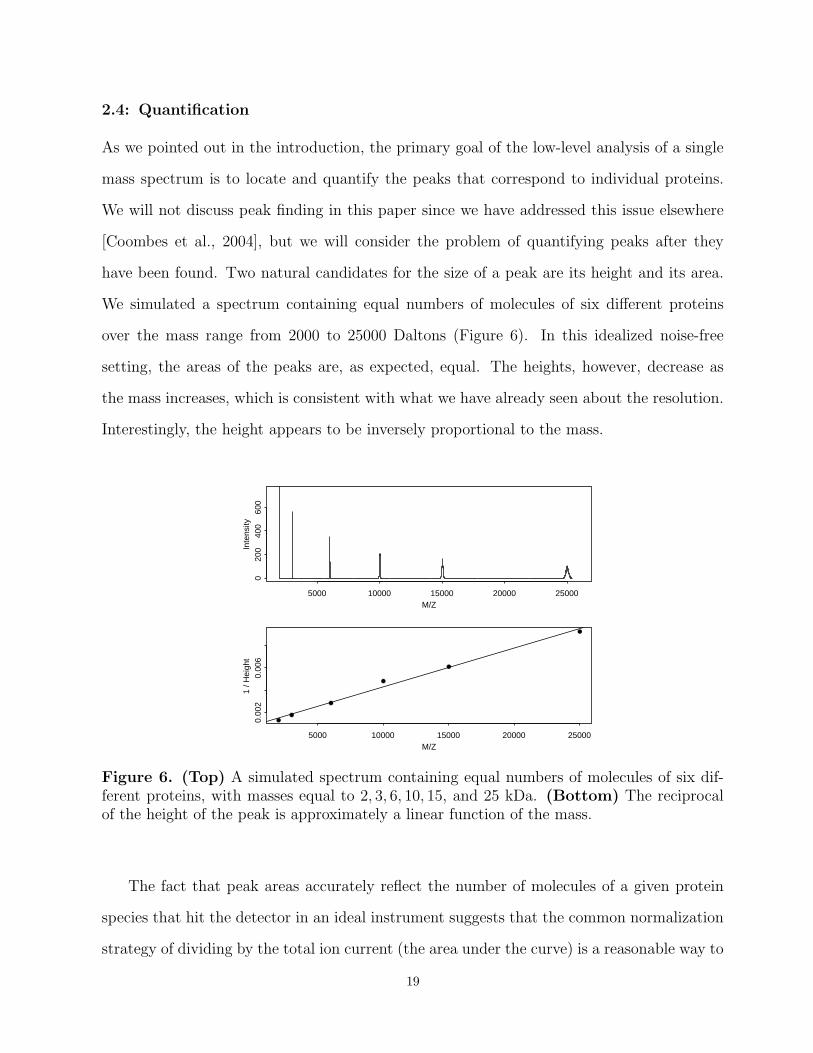
2.4: Quantification

As we pointed out in the introduction, the primary goal of the low-level analysis of a single

mass spectrum is to locate and quantify the peaks that correspond to individual proteins.

We will not discuss peak finding in this paper since we have addressed this issue elsewhere

[Coombes et al., 2004], but we will consider the problem of quantifying peaks after they

have been found. Two natural candidates for the size of a peak are its height and its area.

We simulated a spectrum containing equal numbers of molecules of six different proteins

over the mass range from 2000 to 25000 Daltons (Figure 6). In this idealized noise-free

setting, the areas of the peaks are, as expected, equal. The heights, however, decrease as

the mass increases, which is consistent with what we have already seen about the resolution.

Interestingly, the height appears to be inversely proportional to the mass.

M/Z

Inte

nsity

5000 10000 15000 20000 25000

020

040

060

0

M/Z

1 / H

eigh

t

5000 10000 15000 20000 25000

0.00

20.

006

Figure 6. (Top) A simulated spectrum containing equal numbers of molecules of six dif-ferent proteins, with masses equal to 2, 3, 6, 10, 15, and 25 kDa. (Bottom) The reciprocalof the height of the peak is approximately a linear function of the mass.

The fact that peak areas accurately reflect the number of molecules of a given protein

species that hit the detector in an ideal instrument suggests that the common normalization

strategy of dividing by the total ion current (the area under the curve) is a reasonable way to

19

account for differences in the total amount of sample protein that was applied to the sample

plate.

3: Discussion

In this article, we have described some preliminary results using a simulation of mass spectra

based on a physical model of a linear MALDI-TOF instrument with time-lag focusing. We

have shown that our simulation recovers some of the important characteristics of real data.

We expect the simulation to be a useful tool in developing improved methods for processing

and analyzing mass spectrometry data, since it will allow us to generate complex spectra

where the true locations and sizes of the peaks are known. The simulation code in S-Plus is

available from our web site (http://bioinformatics.mdanderson.org/cromwell.html).

Some recent analyses of SELDI spectra have used every measured time point (or every

m/z value) as a potential feature used to build a classifier to distinguish cancer samples

from normal samples [Petricoin et al., 2002; Zhu et al, 2003]. We believe that this approach

is misguided. As we have seen, the spread in initial velocities and the isotope distribution

can cause the measurement of a single protein to extend over many time points. From a

biophysical perspective, it seems unreasonable to treat things that cannot possibly be distin-

guished within the resolution of the instrument as independent entities. From a statistical

perspective, complications arise when one treats highly correlated measurements as though

they were independent. These statistical difficulties are compounded by the tremendous

amount of multiple testing that accompanies the selection of a few features out of several

thousand m/z values.

We can perform a simple calculation to get an idea of how many peaks can be resolved

in a spectrum. The “peak capacity” of a mass spectrum is defined as the maximum number

N of peaks could be distinguished as m/z ranges between a and b with a relative mass error

r. Given perfect spacing of the peaks, the first peak would be found at a, the second at

20

a + ra = (1 + r)a, the third at (1 + r)2a and the last at b = (1 + r)N+1a. Thus, we can

compute the peak capacity explicitly as

N = −1 +log(b/a)

log(1 + r).

As an example, when a = 2000, b = 20000, and r = 0.1%, then the peak capacity is

N = 2303. If the relative mass error degrades to 0.2%, then the peak capacity diminishes

to only 1152, and with a relative mass error of 0.5%, the peak capacity is only 461. It

is interesting to note that, in our experience with SELDI data in this mass range, we can

typically identify between 100 and 200 peaks.

Although we have talked about quantification of peaks in this article, we should make

it clear exactly what is being quantified. Our simulation models those molecules that are

desorbed from the surface, ionized, and detected. Being able to accurately quantify these

molecules is only part of the problem. In an actual experiment, we would like to be able

to quantify the number of molecules of each mass that were deposited on the surface. Un-

fortunately, the selection process that determines which molecules make it off the surface

involves extremely complicated chemical interactions between the analytes and the matrix

and among the analytes. We can (potentially) succeed in making mass spectrometry quan-

tifications more precise, but are likely to be stymied in efforts to make them more accurate.

There are a number of potential enhancements to the simulation model described here.

First, the current model ignores the physics of the detector, which is another source of

stochastic noise in the system. Second, one could try to model a more elaborate instrument.

The obvious next step would be to include a reflectron instead of a simple linear flight path.

Third, we could extend the modeling of the isotope distribution to consider other common

molecule alterations, such as the inclusion of salt adducts or the loss of water molecules.

Fourth, one might want to explicitly model some of the interactions of the paricles in the

plume before the focusing electric field is imposed.

Our eventual goal is, as mentioned above, to simulate complex mixtures of proteins in

order to evaluate the behavior of different methods to process and analyze mass spectra.

21

These simulations are likely to require additional stochastic components beyond the distri-

bution of initial velocities and of isotopes. For example, it is reasonable to believe that the

voltage is essentially constant for all molecules in a single experiment. When simulating

experiments with different samples across laboratories or across time, however, variability in

the nominal voltages (or in the specified delay time) is an additional source of noise. One will

also have to decide how to simulate the background electronic or chemical noise and realistic

baseline curves. Finally, there is the challenge of deciding what kinds of truth (number,

mass, intensity, and variability of peaks) to simulate for the input to the present simulation

engine. We believe that these challenges will eventually be met, and that the simulation tool

described in the presnt article is a useful step in the right direction.

4: Acknowledgements

This research was supported in part by NIH/NCI grants P50 CA070907 and R01 CA107304-

01.

5: References

Adam BL, Qu Y, Davis JW, Ward MD, Clements MA, Cazares LH, Semmes OJ, Schell-

hammer PF, Yasui Y, Feng Z, Wright GL Jr. Serum protein fingerprinting coupled with

a pattern-matching algorithm distinguishes prostate cancer from benign prostate hyper-

plasia and healthy men. Cancer Res. 2002; 62: 3609-3614.

Adam PJ, Boyd R, Tyson KL, Fletcher GC, Stamps A, Hudson L, Poyser HR, Redpath N,

Griffiths M, Steers G, Harris AL, Patel S, Berry J, Loader JA, Townsend RR, Daviet L,

Legrain P, Parekh R, Terrett JA. Comprehensive proteomic analysis of breast cancer cell

membranes reveals unique proteins with potential roles in clinical cancer. J Biol Chem.

2003; 278: 6482-9.

22

Baggerly KA, Morris JS, Wang J, Gold D, Xiao LC, Coombes KR. A comprehensive approach

to the analysis of matrix-assisted laser desorption/ionization-time of flight proteomics

spectra from serum samples. Proteomics. 2003; 3: 1667-72.

Baggerly KA, Morris JS, Coombes KR. Reproducibility of SELDI-TOF protein patterns in

serum: comparing datasets from different experiments. Bioinformatics. 2004; 20: 777-85.

Barbacci DC, Edmondson RD, Russell DH. Evaluation of the variables that affect resolution

in delayed extraction MALDI-TOF. Int J Mass Spectrom Ion Proc. 1997; 165/166: 221-

235.

Beavis RC, Chait BT. Velocity distributions of intact high mass polypeptide molecule ions

produced by matrix assisted laser desorption. Chem Phys Lett. 1991; 181: 479-484.

Christian NP, Arnold RJ, Reilly JP. Improved calibration of time-of-flight mass spectra by

simplex optimization of electrostatic ion calculations. Anal Chem. 2000; 72: 3327-37.

Coombes KR, Fritsche HA Jr, Clarke C, Chen JN, Baggerly KA, Morris JS, Xiao LC, Hung

MC, Kuerer HM. Quality control and peak finding for proteomics data collected from

nipple aspirate fluid by surface-enhanced laser desorption and ionization. Clin Chem.

2003; 49: 1615-23.

Coombes KR, Tsavachidis S, Morris JS, Baggerly KA, Hung MC, Kuerer HM. Improved peak

detection and quantification of mass spectrometry data acquired from surface-enhanced

laser desorption and ionization by denoising spectra with the undecimated discrete wavelet

transform. M.D. Anderson Biostatistics Technical Report UTMDABTR-001-04. 2004.

Gluckmann M, Karas M. The initial ion velocity and its dependence on matrix, analyte and

preparation method in ultraviolet matrix-assisted laser desorption/ioinization. J Mass

Spectrom. 1999; 34: 467-477.

Hack CA, Benner WH. A simple algorithm improves mass accuracy to 50-100 ppm for

delayed extraction linear matrix-assisted laser desorption/ionization time-of-flight mass

spectrometry. Rapid Commun Mass Spectrom. 2002; 16: 1304-12.

23

Hawkins DM, Wolfinger RD, Liu L, Young SS. Exploring blood spectra for signs of ovarian

cancer. Chance. 2003; 16: 19-23.

Ingendoh A, Karas M, Hillenkamp F, Giessmann U. Factors affecting the resolution in matrix-

assisted laser desorption-ionization mass spectrometry. Int J Mass Spectrom Ion Proc.

1994; 131: 345-354.

Juhasz J, Vestal ML, Martin SA. On the initial velocity of ions generated by matrix-asisted

laser desorption ionization and its effect on the calibration of delayed extraction time-of-

flight mass spectra. J Am Soc Mass Spectrom. 1997; 8: 209-217.

Lee KR, Lin X, Park DC, Eslava S. Megavariate data analysis of mass spectrometric pro-

teomics data using latent variable projection method. Proteomics. 2003; 3: 1680-6.

Liggett W, Cazares L, Semmes OJ. A look at mass spectral measurement. Chance. 2003;

16: 24-28.

Merchant M, Weinberger SR. Recent advancements in surface-enhanced laser desorption/

ionization-time of flight-mass spectrometry. Electrophoresis. 2000; 21: 1164-77.

Paweletz CP, Gillespie JW, Ornstein DK, Simone NL, Brown MR, Cole KA, Wang QH,

Huang J, Hu N, Yip TT, Rich WE, Kohn EC, Linehan WM, Weber T, Taylor P, Emmert-

Buck MR, Liotta LA, and Petricoin EF. Rapid protein display profiling of cancer pro-

gression directly from human tissue using a protein biochip. Drug Development Research

2000; 49: 34-42.

Paweletz CP, Trock B, Pennanen M, Tsangaris T, Magnant C, Liotta LA, Petricoin EF 3rd.

Proteomic patterns of nipple aspirate fluids obtained by SELDI-TOF: potential for new

biomarkers to aid in the diagnosis of breast cancer. Dis Markers. 2001; 17: 301-7.

Petricoin EF, Ardekani AM, Hitt BA, Levine PJ, Fusaro VA, Steinberg SM, Mills GB,

Simone C, Fishman DA, Kohn EC, Liotta LA. Use of proteomic patterns in serum to

identify ovarian cancer. Lancet. 2002; 359: 572-7.

Rai AJ, Zhang Z, Rosenzweig J, Shih IeM, Pham T, Fung ET, Sokoll LJ, Chan DW. Pro-

teomic approaches to tumor marker discovery. Arch Pathol Lab Med. 2002; 126: 1518-26.

24

Schaub S, Wilkins J, Weiler T, Sangster K, Rush D, Nickerson P. Urine protein profiling

with surface-enhanced laser-desorption/ionization time-of-flight mass spectrometry. Kid-

ney Int. 2004; 65: 323-32.

Sorace JM, Zhan M. A data review and re-assessment of ovarian cancer serum proteomic

profiling. BMC Bioinformatics. 2003; 4: 24.

Tang N, Tornatore P, Weinberger SR. Current developments in SELDI affinity technology.

Mass Spectrom Rev. 2004 Jan-Feb;23(1):34-44.

Vestal ML, Juhasz P, Martin SA. Delayed extraction matrix-assisted laser desorption time-

of-flight mass spectrometry. Rapid Commun Mass Spectrom. 1995; 9: 1044-1050.

Vestal ML, Juhasz P. Resolution and mass accuracy in matrix-assisted laser desorption

ionization time-of-flight. J Am Soc Mass Spectrom. 1998; 9: 892-911.

Wagner M, Naik D, Pothen A. Protocols for disease classification from mass spectrometry

data. Proteomics. 2003; 3: 1692-8.

Wellmann A, Wollscheid V, Lu H, Ma ZL, Albers P, Schutze K, Rohde V, Behrens P,

Dreschers S, Ko Y, Wernert N. Analysis of microdissected prostate tissue with ProteinChip

arrays–a way to new insights into carcinogenesis and to diagnostic tools. Int J Mol Med.

2002; 9: 341-7.

Wiley WC, McLaren IH. Time-of-flight mass spectrometer with improved resolution. Rev

Sci Instruments. 1955; 26: 1150-1157.

Yasui Y, Pepe M, Thompson ML, Adam BL, Wright GL Jr, Qu Y, Potter JD, Winget M,

Thornquist M, Feng Z. A data-analytic strategy for protein biomarker discovery: profiling

of high-dimensional proteomic data for cancer detection. Biostatistics. 2003; 4: 449-63.

Yasui Y, McLerran D, Adam BL, Winget M, Thornquist M, Feng Z. An automated peak

identification/calibration procedure for high-dimensional protein measures from mass spec-

trometers. J Biomed Biotechnol. 2003; 2003: 242-248.

25

Zhang Z, Guan S, Marshall AG. Enhancement of the effective resolution of mas spectra

of high-mass biolmolecules by maximum entropy-based deconvolution to eliminate the

isotopic natural abundance distribution. J Am Soc Mass Spectrom. 1997; 8: 659-670.

Zhu W, Wang X, Ma Y, Rao M, Glimm J, Kovach JS. Detection of cancer-specific markers

amid massive mass spectral data. Proc Natl Acad Sci U S A. 2003; 100: 14666-71.

Zhukov TA, Johanson RA, Cantor AB, Clark RA, Tockman MS. Discovery of distinct protein

profiles specific for lung tumors and pre-malignant lung lesions by SELDI mass spectrom-

etry. Lung Cancer. 2003; 40: 267-79.

26