Embed Size (px)
Citation preview

UNDERSTANDING MAP INTEGRATION USING GIS SOFTWARE
Submitted July 29, 2016
Michelle Pasco
Undergraduate Research Assistant
Civil and Environmental Engineering Department
Old Dominion University
135 Kaufman Hall, Norfolk, VA 23529
E-mail: [email protected]
Total Word Count = 3880 words + 7 Figures * 250 + 4 Tables * 250 = 6630 words

Pasco 2
I. ABSTRACT
Geospatial data stored in Geographical Information Systems (GIS) is beneficial to researchers
because it can relay ground-truth information and numerous datasets can simultaneously be
observed. With the rise of technological advancements, map integration has been introduced
as an innovative technique for studying geographic-enabled data as it can provide a differing
viewpoints and insights on scientific research. Although map integration can be advantageous
in analyzing data, accurate results are difficult to obtain due to spatial displacement and
attribute disparity. These issues include geometric discrepancies, different data structures, and
altered representation. This project focuses on understanding the issues that follow the map
integration process and discovering methods that can increase the accuracy of the process. In
the context of map integration for road networks, two methods, spatial join and transfer
attributes, were studied that were shown to offer favorable and encouraging results. The
research also was able to discern between the cases when one method is more appropriate
than the other.
II. INTRODUCTION
Background: Conflation is an important part of geo-scientific research. It is the integration of
two or more spatial datasets, most of the time represented as maps, and it is used to acquire a
better understanding of the data that cannot be done by researching them individually. There
are two types of map conflation: horizontal and vertical. Horizontal conflation is edge-matching
adjacent maps while removing any differences in spatial content. Vertical conflation is the
combination of two or more maps of the same region that have data structure and thematic
disparity (1). For this project, vertical conflation will be used as the project covers two road
networks of same area, namely the Commonwealth of Virginia. To gather more information
about the geographical data sets, conflating them is often done within GIS and can be made
available for private or public creation and distribution (2). Although map integration is
beneficial, it is susceptible to a number of issues surrounding the process.
Problem: Traffic data is valuable for federal, state, and local governments, businesses, and
engineering. Using traffic geospatial data, several pieces of information (fields) or status reports
can be collected about incidents, weather events and other types of event and can be stored
electronically into one file or an archive (3). Often times there are industries that publish their
individual data sets specific to their demand or research. Users have the ability to integrate
multiple geospatial data using GIS. Although this is beneficial to the user, map conflation faces
difficulties that are not easily resolved. Currently, research is being done on how to correct the
issues by creating semi-automatic or automatic codes, iterations, and equations (4). The issues
that arise during the conflation process are geometrical discrepancies such as differences in

Pasco 3
length, position, direction, size, shape of features; or overlaps, gaps, and duplication in features
(5). There can also be prior process differences such as data structure or in feature
representation.
Faulty data integration begins with one of the following: unequal updating periods, equal data
models acquired by different operators, unequal data models, and content differences (1). The
updating period is critical because in order to maintain accurate map information there may be
continual transformation of the maps in a certain time frame. Two examples would be roadway
reconstruction or natural occurrences such as erosion on shores. Datasets can also have
different operators, which means that the data can be interpreted and represented differently.
Due to this fact, different Geographic Coordinate Systems (GCS) and the present of unique data,
like frontage roads, in only one of the maps can affect the conflation process and ultimately the
accuracy. This also links to conflicting (unequal) data model structures, primarily referring to
the segmentation system. Finally, it is highly unlikely to have datasets that all describe the same
data sets. In previous work, conflation has been done between a geo-scientific dataset and a
topographic dataset resulting in large geometric discrepancies (1). For this project, two road
networks are being conflated that were generated by different industries, and have different
and feature representation, road geometry, and attribute aspects.
Objective: The objective is to improve the conflation process and mitigate the resulting
problems. Unfortunately, spatial displacement aspect is often non-systematic, so it will be
difficult to pinpoint the reasons as to why it conflates inaccurately (2). This project utilizes
previous data and attempts to conflate by using several methods within GIS to further
understand the issues following the integration process.
III. STUDY AREA
Data Sets: The two data sets that were used in conflation in this work were:
VDOT (Virginia Department of Transportation) LRS (Linear Referencing System) road
network, published on August 2015 and available at ArcGIS Online URL here
INRIX XD proprietary road network for Virginia dated December 2014 that was
purchased by VDOT and made available to the researchers.
In addition to these data sets, Google Earth from January 2016 and Google Maps from 2016
were used to aid in the conflation process when the discrepancies between the two data sets to
be conflated could not be immediately resolved.
Study Area: The Virginia road network was studied with specific focus on five interstates: I-64,
I-564, I-95, I-395, and I-495. These interstates pass through three urban regions including

Pasco 4
Hampton Roads (HR), Richmond, and Northern Virginia (NOVA). The rural areas are along the
two main interstates, I-64 and I-95 outside of the three urban areas.
Figure 1: Study Area Map
I-64 runs from the east coast of Virginia into West Virginia. It passes through Hampton Roads,
which includes cities such as Hampton, Norfolk, Virginia Beach, and Chesapeake. I-564 is a
branch from I-64 which connects the Norfolk Naval Base to downtown Norfolk. I-64 also runs
through Virginia’s capital, Richmond, which is where I-95 and I-64 intersect. In Virginia I-95 runs
from NOVA to the North Carolina border. NOVA includes cities such as Alexandria, Arlington,
and Manassas and is within close proximity to the nation’s capital, Washington D.C. Interstate
I-395 runs from I-95/I-495/I-395 Springfield-Franconia Interchange to the Washington DC. In
this project, I-495 denotes only the Virginia section of the Capital Beltway. As mentioned
before, for the purpose of this project, all areas along I-64 and I-95 that are outside of the three
urban cities will be considered rural.
IV. METHODOLOGY
Data: The first step was to understand the issues surrounding map migration and applying that
understanding to the two data sets. We studied two different data sources: Virginia
Department of Transportation’s (VDOT) Linear Referencing System (which from now on will be
called “LRS” in this paper) and INRIX XD (which will be called from now on “XD” in this paper).
The VDOT LRS map data is public and is it used by the private sector and the general public to
study VDOT maintained roadways and compile business data (5). The map document is updated
quarterly to ensure accurate road networks by eliminating previous geometric discrepancies
and adjusting old roads.
Within the LRS, the road segments are defined by a start and end point. The LRS also contains
multiple layers, within GIS, that contain different attributes for unique purposes. This project
used the specific layer called “SDE_VDOT_EDGE_RTE_OL_MPST_LRS”. Here the layer name
Pasco 5
stands for “Spatial Database Engine (SDE) VDOT EDGE (segmentation system) Route (RTE)
Overlap (OL) Milepost (MPST) LRS.” The segments are based off of mileposts displayed in
Virginia. The LRS contains all the VDOT-maintained roads in Virginia. The features in this layer of
the LRS are road links, usually directional and short in length, that are broken at significant
points in the geometry of the road.
INRIX is a company that provides traffic data and services through connected devices that
include road speed parameters, incident information, and text alerts . The speed and travel time
information is based mainly on vehicle probes (1). This information is delivered based on
geographical links called XD segments, which define specific sections of roadways (6). XD’s road
system is not as specific as LRS and only provides certain roads that are within LRS’s secondary
and urban roads for which INRIX can collect probe data. Like the LRS links, the XD links are
directional and short in length and are broken at logical points. Generally, the XD links are
shorter than 1.5 miles, but many of them are longer than LRS links.
VDOT also provided a sample conflation between the LRS and XD road networks. When
observing this sample conflation, it was apparent that it had gaps and overlaps. After further
research and cross referencing with Google Earth and Google Maps, it was concluded that
possible reasons for these issues might have included disjointed segmentation in the road
geometry, road geometric disparity, mismatched attributes, and outdated information. To
further understand these issues, this project attempted to perform a conflation of the five
study area roadways using several methods in GIS:
Spatial Join (with variants of same and different GCS and EDGE- vs. non-EDGE matching),
Transfer Attributes,
Other methods (edge-matching and join by attributes).
All the analysis for this work was done using the ESRI ArcGIS software suite.
Spatial Join: Spatial join is joining features by intersecting their geometry (7). Dataset objects
are digitized with vector components such as points, lines, and polygons. With this tool, the
vector components for each of the two datasets become either the “source” or “target” layer.
After the spatial join conflation process, an output field called “Count_” is created on the
attribute table. This “Count_” is the number of intersections (or matches) that each feature has.

Pasco 6
Figure 2: The "Count_" field is shown in light blue. 0 indicates that the feature did not match with any other features.
In this project, the LRS was set as the source layer and the XD was set as the target layer. In an
attempt to increase the accuracy, the influence of two factors was studied. The first factor was
the geographical coordinate system, with the possibilities of keeping the original GCS and
converting to a common GCS. In the first case, the spatial join was performed with the LRS and
XD in their respective original GCSs. LRS had “GCS_North_American_1983” GCS and XD had
“GCS_WGS_1984” GCS as their original GCS. In the second attempt the same GCS was used for
both datasets. XD’s GCS was projected to match the LRS’s GCS using the Project tool under Data
Management Toolbox in GIS.
The second factor was the layer within the LRS: EDGE and Non-EDGE. EDGE means that the
roads are broken up into multiple segments to increase accuracy of the road geometry. “Non-
EDGE” means that the road is made of a two segments with each segment bearing the direction
of the road. For example, I-64’s two segments are labeled as I-64 west and I-64 east.
Taking into account these two situations, each with two options, four sets of spatial join
conflations were generated in total.

Pasco 7
Figure 3: GCS vs Original (ORG) spatial join case on part of I-64 where the top segments are the source and target layers and the bottom segments are the conflations
To increase the GIS processing speed, each of the spatial joins was done individually for each of
the five interstates. After the completion of each spatial join, the attribute table was analyzed
to see how many features had matches in the “Count_” field. An equation was created to
measure the “Conflation Accuracy” to study the relationship between the count and spatial join
accuracy:
(𝑐𝑜𝑢𝑛𝑡 > 0) 𝑓𝑒𝑎𝑡𝑢𝑟𝑒𝑠
𝑡𝑜𝑡𝑎𝑙 # 𝑜𝑓 𝑓𝑒𝑎𝑡𝑢𝑟𝑒𝑠∗ 100 = 𝑐𝑜𝑛𝑓𝑙𝑎𝑡𝑖𝑜𝑛 𝑎𝑐𝑐𝑢𝑟𝑎𝑐𝑦, 𝑐𝑎 (%)
where count = 0 means that the feature did not match and count > 0 represents the features
that did match. Once each of the study areas for the two comparisons was completed, the
average was taken to discover which of the two was more accurate.
Transfer Attributes: Transfer attributes is joining attributes in one dataset to corresponding
attributes in another dataset (7). Similar to spatial join, there must be a source and target layer.
An additional requirement is that each of the layers needs to have the same GCS. Then, one or
more common attributes between the two datasets are selected along with a search distance
to match features. After the conflation process, the selected field(s) is (are) transferred into the
attribute table of the target layer where it will show the values that have matched with the
source layer values. If <Null> values appear, then it means that the target features failed to
match with the source features.

Pasco 8
Figure 4: The left column is the transferred field from the source layer (LRS) to the target layer (XD).
The LRS was used as the source layer and the XD was used as the target layer. The common
field that was used for matching is called Route Common Name or “RTE_COMMON_NM.” Four
search distances were used were 0.1 mi, 0.3 mi, 0.5 mi, and 1 mi in an attempt to find the one
that would contribute to the most accurate results . These distances were chosen because they
were will within estimated bounds for accurate conflation, yet broad enough to provide a
reasonable sample. For research purposes, 0.05 mi, 2 mi, and 5 mi were also tested but they
yielded poor conflation results and so they were discarded. After recording the data, a similar
equation to spatial join was used to calculate the conflation accuracy:
𝑛𝑜 < 𝑁𝑢𝑙𝑙 > 𝑓𝑒𝑎𝑡𝑢𝑟𝑒𝑠
𝑡𝑜𝑡𝑎𝑙 # 𝑜𝑓 𝑓𝑒𝑎𝑡𝑢𝑟𝑒𝑠∗ 100 = 𝑐𝑜𝑛𝑓𝑙𝑎𝑡𝑖𝑜𝑛 𝑎𝑐𝑐𝑢𝑟𝑎𝑐𝑦, 𝑐𝑎 (%)
where “no <Null>” means that the features that did not match were removed to only include
the features that did match.

Pasco 9
Figure 5: Comparison between 0.1 mi and 0.3 mi conflations for transfer attributes on part of I-64 where the top segments are the source and target layers and the bottom segments are the conflations.
To further understand how the search distance affects the conflation result, the buffer tool was
used to visually observe the relationship between the search distance and roads. The tool
creates a buffer surrounding a feature that is determined by the search distance (7). First, the
source layer was LRS and the target feature was XD. Additionally, the analysis was completed in
the reverse order. Buffer has two types: round and flat. Round buffer surrounds the segment
with a radial buffer, while a flat buffer creates one that terminates at the endpoint.
Figure 6: The top segment represents each of the round buffers and the bottom segment represents the flat buffer.
Other methods: The two other methods that were tested are called “edge-matching” and “join
by attributes.” Edge-match is a tool that physically transforms features during the conflation
process (7). Prior to using the edge-match tool, a separate tool called “generate edge-match
links” is required to assess each of the segment features. These tools need a source layer,
target layer, and require that the source and target layers have identical GCS. After using the
generate edge-match tool, an output table is created including start and end points of each
segments and an “edge-match confidence” or “em_conf.” Edge-match confidence scores each

Pasco 10
of the features on a value range of 0 to 100, 100 being the maximum confidence level. The
lower the confidence level, the less likely the segment will conflate. The project does not
include the edge-match tool because a great deal of manual intervention is needed to
transform the segments with low confidence levels to increase the accuracy. This is not suitable
for large-scale projects.
Join by attributes is similar to transfer attributes, but it forces users to choose two fields, one in
each of the datasets, in order to conflate (7). To conflate, the fields are not required to have the
same GCS, but the tool still needs a source and target layer. The process joins the source layer’s
attribute table to the target layer’s attribute table, attempting to match corresponding
features. If there is no correlation between the layers, the target dataset’s attribute table will
be recorded as a <Null> value. The project did not utilize the join by attributes because it is
difficult to acquire two fields that will match the features within two datasets and involves
several rounds of trial and error. The common result is that all of the target attribute table will
be <Null>.
V. RESULTS
Spatial Join: The table below displays the result of 20 spatial joins for the four cases.
Table 1: Spatial join results.
Road Name & Spatial Join Type
# of features
Count>0 features
Conflation Accuracy,
ca (%) Average ca
64_EDGE_ORG 728 632 86.81
75.11
564_EDGE_ORG 12 10 83.33
95_EDGE_ORG 573 452 78.88
395_EDGE_ORG 136 89 65.44
495_EDGE_ORG 167 102 61.08
64_EDGE_GCS 728 359 49.31
44.11
564_EDGE_GCS 12 10 83.33
95_EDGE_GCS 573 287 50.09
395_EDGE_GCS 136 27 19.85
495_EDGE_GCS 167 30 17.96
64_NON_ORG 2 2 100.00
100.00
564_NON_ORG 2 2 100.00
95_NON_ORG 2 2 100.00
395_NON_ORG 2 2 100.00
495_NON_ORG 2 2 100.00
64_NON_GCS 2 2 100.00 100.00

Pasco 11
564_NON_GCS 2 2 100.00
95_NON_ GCS 2 2 100.00
395_NON_ GCS 2 2 100.00
495_NON_ GCS 2 2 100.00
Where:
The number represents the interstate
“EDGE” represents the EDGE layer in LRS
“ORG” represents the original XD
“GCS” represents the Geographic Coordinate System or the projected XD layer
“NON” represents the Non-EDGE layer in LRS.
In the GCS versus ORG cases, the recorded data shows that the ORG is 30% more accurate in
the EDGE layer and there is no difference in the Non-EDGE layer. In the EDGE versus Non-EDGE
cases, Non-EDGE is 100% accurate due to the fact that there are only two segments for each
interstate. Although Non-EDGE seems to be complete, the XD matched with the entire road
instead of a segment on the LRS. This will not be sufficient for many applications that would use
the conflated datasets. Since both Non-EDGE comparisons resulted identically, further
investigation of the count for each feature was done.
Table 2: NON-EDGE segments count results.
Road Name & Spatial Join Type First Segment
Match Count Second Segment
Match Count
64_NON_ORG I-64E 628 I-64W 620
564_NON_ORG I-564E 9 I-564W 15
95_NON_ORG I-95S 443 I-95N 438
395_NON_ORG I-395S 84 I-395N 96
495_NON_ORG I-495S 77 I-495N 79
64_NON_GCS I-64E 190 I-64W 208
564_NON_GCS I-564E 4 I-564W 2
95_NON_GCS I-95S 127 I-95N 146
395_NON_GCS I-395S 12 I-395N 23
495_NON_GCS I-495S 9 I-495N 7
In the table above N, S, E, and W are North, South, East, and West, respectively. According to
the data, the ORG layer receives more matches than the GCS layer. The greater the count
number is, the more trouble GIS will have matching the correct segments. Although it may
seem that ORG is less accurate than GCS, there is a chance that it is actually the opposite. GCS is
Pasco 12
less accurate because projecting a shape file to a different GCS induces geometric
discrepancies. Therefore, it was concluded that the main reason behind the NON_GCS case
having a lower count is because GIS is not reading the segments correctly.
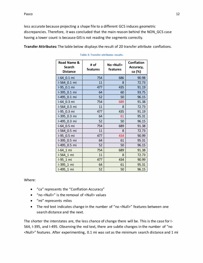
Transfer Attributes: The table below displays the result of 20 transfer attribute conflations.
Table 3: Transfer attributes results.
Road Name & Search
Distance
# of features
No <Null> features
Conflation Accuracy,
ca (%)
I-64_0.1 mi 754 686 90.98
I-564_0.1 mi 11 8 72.73
I-95_0.1 mi 477 435 91.19
I-395_0.1 mi 64 60 93.75
I-495_0.1 mi 52 50 96.15
I-64_0.3 mi 754 689 91.38
I-564_0.3 mi 11 8 72.73
I-95_0.3 mi 477 435 91.19
I-395_0.3 mi 64 61 95.31
I-495_0.3 mi 52 50 96.15
I-64_0.5 mi 754 689 91.38
I-564_0.5 mi 11 8 72.73
I-95_0.5 mi 477 434 90.99
I-395_0.5 mi 64 61 95.31
I-495_0.5 mi 52 50 96.15
I-64_1 mi 754 689 91.38
I-564_1 mi 11 8 72.73
I-95_1 mi 477 434 90.99
I-395_1 mi 64 61 95.31
I-495_1 mi 52 50 96.15
Where:
“ca” represents the “Conflation Accuracy”
“no <Null>” is the removal of <Null> values
“mi” represents miles
The red text indicates change in the number of “no <Null>” features between one
search distance and the next.
The shorter the interstates are, the less chance of change there will be. This is the case for I-
564, I-395, and I-495. Observing the red text, there are subtle changes in the number of “no
<Null>” features. After experimenting, 0.1 mi was set as the minimum search distance and 1 mi

Pasco 13
as the maximum search distance due to the fact that anything lower or higher than the
minimum and maximum produced inaccurate results.
Particularly on I-64, three segments matched only 0.3 mi or higher. To understand why this is,
the buffer tool was utilized to mimic how GIS processes the conflation.
Each of the LRS segments were numbered 1 thru 4 from left to right and the number of lines
that intersected with the buffer was recorded. The intersections will be referred to as matches.
The first set of results are matched using the round buffer and setting the source layer as LRS
and target layer as XD with the three search distances being 0.1 mi, 0.3 mi, and 0.5 mi. A single
flat buffer was applied with a search distance of 0.1 mi because it was apparent that the
matches would all be identical. The second case is using the same source and target layers, but
matching which XD segments intersected the buffers. The XD segments are labeled as their
feature number. The results are as followed:
Table 4: Buffer tool results.
LRS Segment
Search Distance
Round Buffer 0.1 mi
Round Buffer 0.3 mi
Round Buffer 0.5 mi
Flat Buffer 0.1 mi
LRS Segment 1 1 1 1 1
LRS Segment 2 3 3 3 2
LRS Segment 3 2 2 2 2
LRS Segment 4 2 2 2 1
XD Segment
Round Buffer 0.1 mi
Round Buffer 0.3 mi
Round Buffer 0.5 mi
Flat Buffer 0.1 mi
XD Segment 1 (4100330)
2 2 2 2
XD Segment 2 (4100331)
3 3 3 2
XD Segment 3 (4100515)
3 3 3 2
In the table above the numbers represent the number of matches for search distance and the
buffer. Observing the results in Figure 7, the 0.1 mi round buffer intersects some of the XD
segments by an insignificant amount. When the buffer search distance is increased to 0.3 mi or
0.5 mi, GIS has enough data to read the features and correctly match.
VI. CONCLUSIONS & OUTLOOK
Understanding the different methods of conflation is crucial in measuring the accuracy of the
process. There are a few methods that are suitable for all types of research. Spatial joining is

Pasco 14
better to use if the data sets are comprised of many, potentially small, features or if the
datasets are comparatively similar in geometry and data structure. Transfer attributes is overall
more accurate because it matches features by not only their geometry, but also by how similar
their attributes are. This method covers the two most important aspects in the conflation
process.
Analyzing the five roadways from the study areas, it can be noted that the smaller interstates (I-
395, I-495, and I-564) seem to be more accurate than the two main interstates (I-64 and I-95).
While observing how the conflation process affected areas along the roads, it seems that there
are more gaps within the urban cities than the rural areas. The most likely cause for this is
because the roads are within close proximity of each other, so they are more likely to be
mismatched by GIS. There are few gaps and overlaps along the rural areas that are due to
geometric discrepancies or mislabeling of road names.
In the future, these methods can be used on a wider scale. For example, instead of doing the
five interstates, the entire Virginia road network can be studied. The side effects of working on
a larger scale will likely be that the conflation process will take much longer and that the
resulting road networks are most susceptible to problems such as gaps and overlaps. This is
because the closer the geometric features are, the higher the mismatching chance is. To
combat these issues, an understanding of the problems that are affiliated with the gaps and
overlaps is required. Manual intervention, such as manually transforming segments, may be
needed for some spots that are not correctly digitized. Once these issues are pinpointed and
resolved, a quasi-automatic or automatic process can be coded and used in GIS. This will create
a smoother conflation process and make it easier for spatial data and attributes for multiple
datasets to be researched.
VII. ACKNOWLEDGEMENTS
A special thanks to Simona Babiceanu, who advised me and kept me on the right path during
my research. I want to also thank Dr. Emily Parkany for the constant support and
encouragement that she gave to me and the other interns. Lastly, I want to give a warm thank
you to Daniela Gonzales for motivating me to apply for the Mid-Atlantic Transportation
Sustainability Center – University Transportation Center (MATS UTC) program.
VIII. REFERENCES
1. G. v. Gösseln, M. Sester. Integration of Geoscientific Data Sets and the German Digital Map
Using A Matching Approach. Commission IV, WG IV/7.
http://www.cartesia.org/geodoc/isprs2004/comm4/papers/534.pdf. Accessed June 15, 2016.
2. Davis, Curt H., Haithcoat, Timothy L., Keller, James M., Song, Wenbo. Relaxation-Based Point
Feature Matching for Vector Map Conflation, 2011. Transactions in GIS, 15(1), pg. 43-60.
Pasco 15
http://onlinelibrary.wiley.com/doi/10.1111/j.1467-9671.2010.01243.x/full. Accessed June 20,
2016.
3. Virginia Department of Transportation. Roadway Network System. Release Notes, Linear
Referencing System, Version 15.2, 2015.
https://www.arcgis.com/home/item.html?id=60916ea827544412ad209ea5192ad7fd. Accessed
June 2, 2016.
4. Haunert, Jan-Henrik. Link based Conflation of Geographic Datasets, 2005.
http://citeseerx.ist.psu.edu/viewdoc/download?doi=10.1.1.615.9696&rep=rep1&type=pdf.
Accessed June 15, 2016.
5. Kang, Hoseok. Geometrically and Topographically Consistent Map Conflation for Federal and
Local Governments, 2004. Journal of the Korean Geographical Society, Vol. 39, No. 5, pg. 804-
818.
http://www.kgeography.or.kr/homepage/kgeography/www/old/publishing/journal/39/05/07.P
DF. Accessed June 14, 2016.
6. INRIX. I-95 Vehicle Protection Project II Interface Guide, 2014.
http://i95coalition.org/projects/vehicle-probe-project/. Accessed June 17, 2016.
7. Environmental Systems Research Institute (ESRI). ArcGIS for Desktop, 2016. arcgis.com. Accessed
July 18, 2016.
8. Doytsher, Yerahmiel, Filin, Sagi, Ezra, Eti. Transformation of Datasets in a Linear-based Map
Conflation Framework, 2001. Surveying and Land Information Systems, Vol. 61, No. 3, pg. 159-
169.
http://www.lr.tudelft.nl/fileadmin/Faculteit/LR/Organisatie/Afdelingen_en_Leerstoelen/Afdelin
g_RS/Optical_and_Laser_Remote_Sensing/Publications/Papers/018-
2001/doc/filin_map_conf_transformation.pdf. Accessed June 14, 2016.