Understanding European Unemployment

with Matching and Search-Island Models

Lars Ljungqvist Thomas J. Sargent∗

July 16, 2007

Abstract

To understand European and American unemployment during the last 60 years, weuse a search-island model and four matching models with workers who have heteroge-neous skills and entitlements to government benefits. When there is higher turbulence,in the sense of worse skill transition probabilities for workers who suffer involuntarylayoffs, high government mandated unemployment insurance (UI) and employment pro-tection (EP) in Europe increase unemployment rates and durations. But when thereis lower turbulence, high European EP suppresses unemployment rates despite highEuropean UI. Four matching models differ in how they assign unemployed workers tomatching functions. That affects how strongly unemployment responds to increasesin turbulence. Heterogeneity among unemployed workers highlights the central roleof adverse labor market externalities in matching models and reveals that the cost ofposting vacancies is the lynchpin of a matching model.

Key words: Job, search, matching, skills, turbulence, discouraged worker, labor marketexternality, bargaining, unemployment, unemployment insurance, employment protection.

∗Ljungqvist: Stockholm School of Economics and New York University (email: lars.ljungqvist@hhs.se);Sargent: New York University and Hoover Institution (email: thomas.sargent@nyu.edu). We are thankful toRiccardo Colacito, Constantino Hevia, Kevin Kallock, Sagiri Kitao, and Alejandro Rodriguez for excellentresearch assistance. For useful comments on earlier drafts, we thank Gadi Barlevy, Marco Bassetto, JeffreyCampbell, Mariacristina De Nardi, Wouter DenHaan, David Domeij, Jesus Fernandez-Villaverde, TimothyKehoe, Narayana Kocherlakota, Dirk Krueger, Lisa Lynch, Edward C. Prescott, Richard Rogerson, FrancoisVelde, anonymous referees, and especially David Backus. We also thank seminar participants at GeorgetownUniversity, New York University, the Federal Reserve Banks of Chicago and New York, ITAM, the Stock-holm School of Economics, the University of Helsinki, the University of Oregon, and the European UniversityInstitute. Ljungqvist’s research was supported by a grant from the Jan Wallander and Tom Hedelius Foun-dation. Sargent’s research was supported by a grant to the National Bureau of Economic Research from theNational Science Foundation.

1

1 Introduction

This paper applies a search-island model and a suite of matching models to understand somestriking differences in European and American unemployment across two broad subperiodsof the twentieth century that we summarize in section 1.1. The models use a human capitalrisk and how it has changed over time to explain the macroeconomic facts in section 1.1,thereby telling a story about the interaction of institutions and the distribution of microe-conomic shocks that Ljungqvist and Sargent (2007a) told with a McCall search model. Butthose similarities in macroeconomic outcomes conceal important differences in the models’microeconomic forces and the personal experiences of the workers who live within them. Forexample, in the matching models, unemployed workers are victimized by the actions of otherworkers who impose adverse congestion externalities, via a matching function, and by theirown bargaining power when firms seek to recoup sunk hiring costs. But in the search-islandmodel, with average luck, unemployed workers are fully responsible for their own situations.Applying these different models as we do is a good way to reveal what makes them tick.

We view it as a point in their favor that these models succeed in explaining the section 1.1facts that have long puzzled macroeconomists. In Ljungqvist and Sargent (2007b), we explainwhy a representative family employment lotteries model is less successful in accomplishingthis particular task.

1.1 Facts

As targets, we take the following facts about unemployment outcomes in two continents:1

1. In the 1950s and 1960s, unemployment rates were persistently lower in Europe than inthe U.S. The difference was accounted for by a higher inflow rate into unemploymentin the U.S.

2. After the 1970s, unemployment became persistently higher in Europe.2

3. Inflow rates into unemployment were roughly constant across periods within both Eu-rope and U.S.

4. In Europe, average durations of unemployment were low in the 1950s and 1960s, butbecame high after the 1970s. Average duration in the U.S. stayed low.

1These facts are documented by Layard et al. (1991).2A proper account of unemployment would include a wider group of people than those officially counted

as unemployed. OECD (2003, chapter 4) reports comprehensive measures of benefit dependency: “Somecountries have now reached a position where most of the working-age population that is neither employed norparticipating in education has an income-replacement benefit. . . . Benefit recipients are a very heterogeneousgroup. Some of them may want to work, or can be ‘activated’ . . . The largest categories in 1999 weredisability, unemployment and [early retirement] . . . a near-universal rise in the aggregate benefit dependencyrate among the population of working age between 1980 and 1990, with Japan and the United States beingthe only exceptions.”

2

5. In Europe, since the 1970s, hazard rates of leaving unemployment fall with increasesin the duration of unemployment.

Next, as features that differentiated Europe and the U.S. and that we shall take asexogenous inputs into the models, we note the following facts about UI and EP:

1. In both periods, government supplied unemployment insurance (UI in the language ofMortensen and Pissarides (1999)) were generous with long durations in Europe, butthey were stingy with short durations in the U.S.

2. Government mandated employment protection (EP in the language of Mortensen andPissarides (1999)) was stronger in Europe throughout both periods.

As in Ljungqvist and Sargent (2007a), we accept the judgement of Krugman (1987) thathigher UI and EP were in place throughout both periods and so take model parameters thatgovern UI and EP to be constant across model subperiods. Of course, to explain differentoutcomes in different subperiods, the models require that some exogenous variable changedacross subperiods. We take this to be something that we call microeconomic turbulence.

In Ljungqvist and Sargent (2007a), we appeal to the following sources of evidence tosupport the hypothesis that turbulence increased after the 1970s:

1. Displaced workers studies document substantial human capital destruction after invol-untary job loss (Jacobson et al. (1993), Farber (1997, 2005)).

2. There is evidence of increased volatility of earnings (Gottschalk and Moffitt (1994),Katz and Autor (1999)).

3. There has been an increase in occupational and industry mobility (Kambourov andManovskii (2005)).

4. A sophisticated observer recently summarized the evidence by noting: “A growingbody of evidence points to the fact that the world economy is more variable and lesspredictable today than it was 30 years ago.. . . [there is] more variability and unpre-dictability in economic life . . .” Heckman (2003, pp. 30–31).

In our models, we define an increase in turbulence as an increase in the probability that aninvoluntarily displaced worker loses human capital.

1.2 Models

Our models tell how high levels of UI and EP interact with an increase in the probability ofskill deterioration after involuntary layoffs. The models share the same stochastic skill accu-mulation and deterioration technologies, but differ with respect to labor market frictions. Inthe search-island model, depending on their financial assets, human capital, and entitlementto benefits, some people spend more time unemployed than others because they exert less

3

effort searching. In the matching models, workers without jobs wait in one or more matchingfunctions. Each model has a theory of a job and of why unemployed workers choose to spendtime in an activity that can be called unemployment.3

1.2.1 Search-island model

The search-island model descends from models of Lucas and Prescott (1974) and Alvarezand Veracierto (2001) and features a search friction and incomplete risk sharing through self-insurance against both unemployment and uncertain life spans after retirement. The modelhas risk averse workers whose decisions about how intensively to search when unemployeddepend on their skills and benefit entitlements as well as on their accumulations of a risk-freeasset, the only available savings vehicle. The wage rate is determined in a competitive labormarket but is constrained to remain fixed in the face of idiosyncratic productivity shocks.Workers receive a fixed wage per unit of skill for the duration of a job.4

1.2.2 Matching models

These models feature a matching function that sets the probabilities at which firms and un-employed workers meet bilaterally as functions of the sizes of pools of workers and firms whoare waiting for invitations to match. An invisible hand adjusts sizes of pools of unemployedworkers and job vacancies to reconcile the choices of workers and firms. Individual workersand firms within each pool face a constant probability of encountering a vacancy and anunemployed worker, respectively.5 To highlight the economic forces at work, we construct asuite of matching models that are differentiated by how they group unemployed workers, inparticular, by whether they put workers with heterogeneous skills and benefit entitlementsinto the same pool or into different pools. Our matching models have risk neutral workers,an attenuated allocative role for wages, and a significant allocative role for the ratio of va-cancies to unemployed workers.6 They feature adverse congestion effects that unemployedworkers impose on each other and that firms with vacancies impose on each other, a wage

3Our models share some limitations. First, they ignore the intensive margin of the labor supply decision byassuming that workers are either unemployed or employed full-time and working the same number of hours.Second, if it were not for the labor market frictions in the matching and search-island models, everyone ofworking age would be employed under laissez-faire. Hence, the models ignore such non-market activities aseducation and child rearing.

4As noted by Alvarez and Veracierto (2001), this greatly simplifies the task of computing an equilibrium.But a consequence is that there are socially wasteful separations.

5Thus, it would be misleading to call these pools ‘queues’.6Hosios (1990) describes the matching framework as follows: “Though wages in the matching-bargaining

models are completely flexible, these wages have nonetheless been denuded of any allocating or signalingfunction: this is because matching takes place before bargaining and so search effectively precedes wage-setting. . . . In conventional market situations, by contrast, firms design their wage offers in competition withother firms to profitably attract employees; that is, wage-setting occurs prior to search so that firms’ offerscan influence workers’ search behavior and, in this way, firms’ offers can influence the allocation of resourcesin the market.”

4

bargaining process, and waiting times as equilibrating signals that reconcile the decisions offirms and workers.

1.3 Organization

Section 2 describes features by all of our models. These include: (1) two transition matricesfor workers’ skill levels, one for workers whose jobs continue or end endogenously, anotherfor workers whose jobs terminate exogenously; (2) a probability distribution from which todraw productivity levels of new workers and transition matrices for the productivity levels ofworkers whose jobs continue; and (3) parameters that define a replacement ratio for UI and alayoff tax for EP. Section 3 describes the additional features that complete the search-islandmodel: a discounted risk-averse utility function that is separable across consumption, searcheffort, time, and states and that imparts a precautionary savings motive; and firm-ownedtechnologies for creating jobs and for converting labor and capital into output. Beyond thecommon features reported in section 2, section 4 describes the additional features in thematching models: a risk-neutral utility function of consumption and four sets of matchingfunctions that define alternative market structures for assigning workers and firms to poolswhere workers wait for jobs and firms post vacancies. Section 5 describes calibrations.Sections 6 and 7 describe outcomes in the search-island and matching models. Section 8describes the perspectives that the models put on the experiences and motives of typicalunemployed European workers. Section 9 contains concluding remarks that by comparingthe key forces at work in our search-island and matching models will remind us of thefollowing message from Lucas and Prescott (1974, p. 206): “The question of whether thereexist important external effects in actual labor markets remains, of course, to be settled.”

Two appendixes describe Bellman equations and equilibrium conditions. A sequel (Ljung-qvist and Sargent 2007b) studies how UI and EP interact with heightened turbulence in arepresentative family employment lotteries model that, while it has complete markets andno labor market frictions, shares with the search-island model the specifications of humanskill accumulation technology, government supplied UI and EP, and firm activities.

2 Common features of our environments

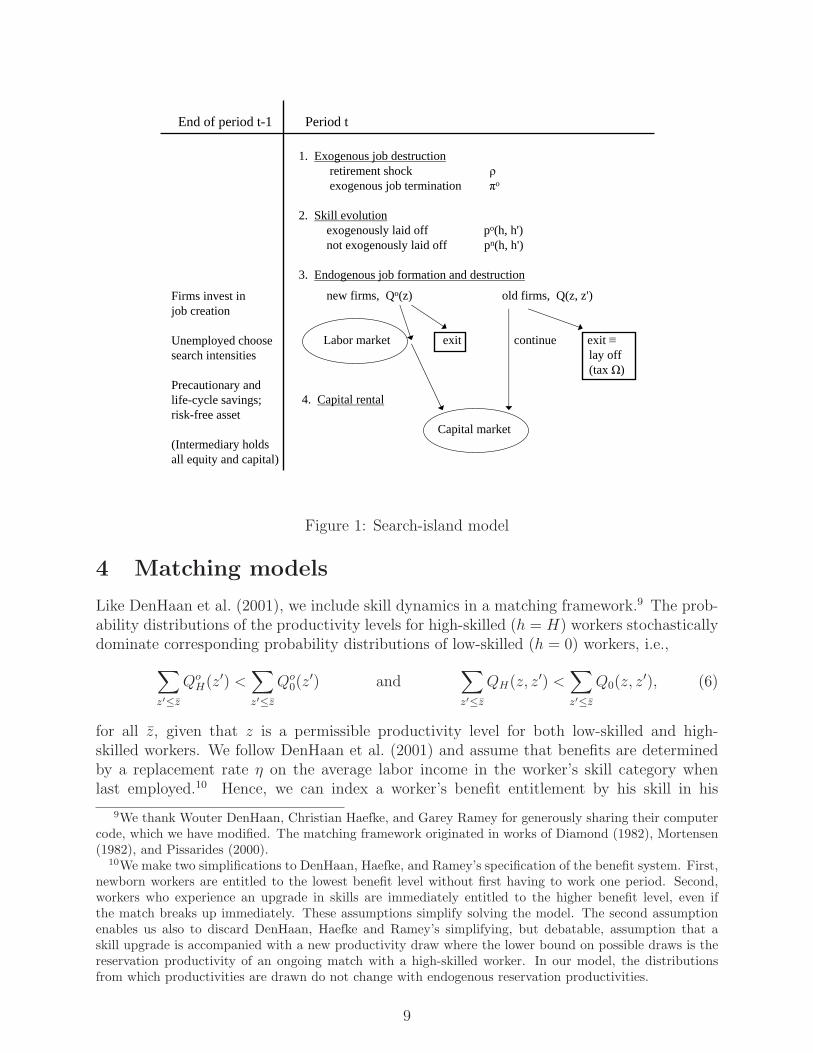
Figures 1 and 2 show the within-period timing of our models. The top halves of these figuresare identical. Each of a continuum of potential workers faces a constant probability ρ ofexiting the labor force. In the matching models, a worker immediately exits the model uponleaving the labor force. In the search-island model, ρ is the probability that a worker willretire and not be allowed to work, and σ is the probability that a retired worker dies. Tokeep the total population and the shares of workers and retirees constant over time, peoplewho die are replaced by newborn workers.

There are three other exogenous sources of uncertainty. First, an employed worker facesa probability πo that his job terminates. Second, workers experience stochastic accumulation

5

or deterioration of skills, conditional on employment status and instances of exogenous jobterminations. Third, idiosyncratic shocks impinge on employed workers’ productivities.

2.1 Skill dynamics

There are two possible skill levels, indexed by h ∈ 0, H. All newborn workers enter thelabor force with the low skill index, h = 0. An employed worker with skill index h faces aprobability pn(h, h′) that his skill at the beginning of next period is h′, conditional on noexogenous job termination. In the event of an exogenous job termination, a laid off workerwith last period’s skill h faces a probability po(h, h′) that his skill becomes h′. A worker’sskill remains unchanged during an unemployment spell. The skill transition matrices are:

pn =

[

1 − πu πu

0 1

]

, (1)

po =

[

1 0πd 1 − πd

]

. (2)

Our notion of turbulence is encoded in the parameter πd ∈ [0, 1], where increased turbulenceis represented as an increase in the parameter value πd.

2.2 Firm formation and productivity

The process of uniting firms and workers differs across the two frameworks but has severalcommon features. Firms incur a cost µ when posting a vacancy in the matching modelor when creating a job in the search-island model. We model a new job opportunity as adraw of productivity z from a distribution Qo

h(z). The productivity of an ongoing job isgoverned by a Markov process: Qh(z, z

′) is the probability that next period’s productivity isz′, given current productivity z. For any two productivity levels z and z < z, the conditionalprobability distribution Qh(z, z

′) first-order stochastically dominates Qh(z, z′), meaning that

∑

z′≤z

Qh(z, z′) <

∑

z′≤z

Qh(z, z′), for all z. (3)

The probability distributions, Qoh(z) and Qh(z, z

′), depend on the worker’s skill h in thematching model, but not in the search-island model.

An employed worker retains his last period productivity with probability (1 − π) anddraws a new productivity with probability π from the distribution Qo

h(z′), so that new

productivities on existing jobs are drawn from the same distribution as the productivities atthe time of job creation; Qo

h(z′) depends on the worker’s current skill index h in the matching

model, but not in the search-island model.

6

2.3 Government mandated UI and EP

The government levies layoff taxes on job destruction and provides benefits to the unem-ployed. It imposes a layoff tax Ω on every endogenous job separation and on every exogenousjob termination except retirement. The government pays unemployment benefits equal to areplacement rate η times a measure of past income. To determine his benefit entitlement,it suffices to keep track of a worker’s skill in his last employment. Newborn workers areentitled to the lowest benefit level in the economy. The government finances unemploymentbenefits with revenues from the layoff tax and other model-specific taxes.

3 Search-island model

Our search-island model with incomplete markets features risk-averse workers who engagein precautionary saving; a non trivial choice of search effort by unemployed workers; and acompetitive labor market for workers whose job searches are successful. The only vehiclefor savings is a single risk-free one-period security. We consign various technical details toappendix A.

We create our model by altering the model of Alvarez and Veracierto (2001).7 We adopttheir specification of a worker’s preferences:

E0

∞∑

t=0

βt

[

log(ct) + A(1 − st)

γ − 1

γ

]

, with A > 0, γ > −1, (4)

where the expectation operator E0 is taken over future states of employment, unemploymentand retirement. β is the subjective discount factor, ct is the worker’s consumption, andst ∈ [0, 1) is the worker’s choice of search intensity if he is unemployed and of workingage. A search intensity st determines an unemployed worker’s probability sξ

t of finding acentralized labor market in the next period, where 0 ≤ ξ ≤ 1. Workers who find the labormarket get a job paying a market-clearing wage rate. To accommodate the feature, notpresent in Alvarez and Veracierto (2001), that workers differ in their skills, we let w denotethe wage rate per unit of skill, where the skill level of a low-skilled worker is normalized toone and the skill level of a high-skilled worker is 1 +H. Hence, a low-skilled worker earns wand a high-skilled worker earns (1 +H)w.

3.1 Firms

We suppress Alvarez and Veracierto’s firm size dynamics and, in the spirit of our matchingmodel, let each firm employ only one worker. Each firm also rents physical capital. The

7The Alvarez and Veracierto (2001) model is descended from the model of Lucas and Prescott (1974) inwhich risk-neutral workers engage in effortless but time-consuming search across a large number of spatiallydistinct islands with idiosyncratic productivity shocks. The only search cost in that model is the opportunitycost of labor income foregone when moving between islands. Alonso-Borrego et al. (2004) use a two-marketversion of the Alvarez and Veracierto (2001) model to study how legal regulations that exempt fixed termlabor contracts from layoff taxes affect equilibrium outcomes.

7

firm’s production function is

ztkαt (1 + ht)

1−α, with α ∈ (0, 1), (5)

where zt is the current productivity level, ht ∈ 0, H is the skill index of the firm’s worker,and kt is physical capital that depreciates at the rate δ. Output can be devoted to consump-tion, investment in physical capital, and startup costs. The rest of Alvarez and Veracierto’smodel of firms enters our framework as follows. Incurring a startup cost µ at time t allows afirm to create a job opportunity at t+1 by drawing a productivity level z from the distribu-tion Qo(z). After seeing z, a firm decides whether to hire a worker from the centralized labormarket. We retain Alvarez and Veracierto’s key assumption that firms and workers first meetunder a veil of ignorance about their partner’s state vector: the firm hires a worker drawnrandomly from a single pool of unemployed workers with a mix of low-skilled and high-skilledworkers. Once hired, a firm observes a worker’s skill, hires the appropriate physical capital,and pays the worker the market wage of w per unit of skill. A firm must retain a worker forat least one period.

We retain Alvarez and Veracierto’s assumption that old as well as new hires earn thesame wage rate (per unit of skill). The assumption that the market-determined wage rateis common to all workers and does not respond to idiosyncratic productivity shocks is re-strictive. To avoid layoffs, workers would be willing to accept wage cuts in response to someadverse productivity shocks.8

3.2 Other features

Besides markets for goods and for renting labor and capital, workers can acquire non-negativeholdings of risk-free assets that earn a net interest rate i. Following Alvarez and Veracierto(2001), we postulate a competitive banking sector that accepts deposits that it invests inphysical capital and claims on firms. The banking sector rents physical capital to firms atthe competitive rental rate i+ δ. Banks hold a diversified portfolio of all firms and thereforebear no risk.

In the spirit of Alvarez and Veracierto, we assume that a worker who dies is replaced bya newborn unemployed worker, to whom he is indifferent, but who nevertheless inherits hisassets. Newborn workers have the low skill index, h = 0.

The government pays unemployment compensation equal to a replacement rate η timesan unemployed worker’s last labor earnings. Newborn workers are entitled to the lowestbenefit level in the economy. The government receives revenues from layoff taxes, and froma flat-rate tax τ on labor earnings and unemployment benefits. The government balancesits budget.

Figure 1 shows the within-period timing of events in our search-island model.

8A main purpose of Alvarez and Veracierto (2001) is to quantify the potential welfare gains of a tax onjob destruction that reduces socially wasteful separations. They acknowledge that the rigidity they imposeon labor contracts and their assumption of no disutility from work cause them to overestimate those welfaregains. While this remains true in our model, notice that the rigidity has no direct effect on the incidence ofskill losses since those are triggered by exogenous job terminations but not by endogenous separations.

8

End of period t-1

Firms invest injob creation

Unemployed choosesearch intensities

Precautionary andlife-cycle savings;risk-free asset

(Intermediary holds all equity and capital)

Period t

1. Exogenous job destructionretirement shock ρexogenous job termination πo

2. Skill evolutionexogenously laid off po(h, h')not exogenously laid off pn(h, h')

3. Endogenous job formation and destruction

new firms, Qo(z) old firms, Q(z, z')

Labor market exit continue exit≡lay off(tax Ω)

4. Capital rental

Capital market

Figure 1: Search-island model

4 Matching models

Like DenHaan et al. (2001), we include skill dynamics in a matching framework.9 The prob-ability distributions of the productivity levels for high-skilled (h = H) workers stochasticallydominate corresponding probability distributions of low-skilled (h = 0) workers, i.e.,

∑

z′≤z

QoH(z′) <

∑

z′≤z

Qo0(z

′) and∑

z′≤z

QH(z, z′) <∑

z′≤z

Q0(z, z′), (6)

for all z, given that z is a permissible productivity level for both low-skilled and high-skilled workers. We follow DenHaan et al. (2001) and assume that benefits are determinedby a replacement rate η on the average labor income in the worker’s skill category whenlast employed.10 Hence, we can index a worker’s benefit entitlement by his skill in his

9We thank Wouter DenHaan, Christian Haefke, and Garey Ramey for generously sharing their computercode, which we have modified. The matching framework originated in works of Diamond (1982), Mortensen(1982), and Pissarides (2000).

10We make two simplifications to DenHaan, Haefke, and Ramey’s specification of the benefit system. First,newborn workers are entitled to the lowest benefit level without first having to work one period. Second,workers who experience an upgrade in skills are immediately entitled to the higher benefit level, even ifthe match breaks up immediately. These assumptions simplify solving the model. The second assumptionenables us also to discard DenHaan, Haefke and Ramey’s simplifying, but debatable, assumption that askill upgrade is accompanied with a new productivity draw where the lower bound on possible draws is thereservation productivity of an ongoing match with a high-skilled worker. In our model, the distributionsfrom which productivities are drawn do not change with endogenous reservation productivities.

9

last employment spell, b ∈ 0, H, so that his benefit entitlement is some function b(b).Let u(h, b) be the number of unemployed workers with current skill h and skill during hisprevious employment spell of b. The total number of unemployed workers is then

u =∑

h,b

u(h, b). (7)

We drop the assumption of DenHaan et al. (2001) that there is an exogenous number offirms and instead impose a zero-profit condition that expresses the outcome of free entry.Let v be the endogenous number of vacancies and let M(v, u) be an increasing, concave, andlinearly homogeneous matching function:

M(v, u) = uM(v

u, 1

)

≡ um(θ), (8)

where the ratio θ ≡ v/u is the endogenously determined degree of “market tightness.” Theprobability of finding a job, M/u = m(θ), is an increasing function of market tightness,and the probability of filling a vacancy, M/v = m(θ)/θ, is a decreasing function of markettightness. We first assume a single matching function for all vacancies and all unemployedworkers, but later consider multiple matching functions.11 For various technical details, seeappendix B.

We form three models with separate matching functions (1) for unemployed workerswith different skill levels, yielding equilibrium vacancies v(h) for each h ∈ 0, H; (2) forunemployed workers having different benefit entitlements, yielding equilibrium vacancies v(b)for each b ∈ 0, H; and (3) for unemployed workers indexed by both their current skill h andtheir skill b in their last employment (as a determinant of their benefit entitlement), yieldingequilibrium vacancies v(h, b) for each pair of values (h, b) ∈ 0, H × 0, H. The last setuprequires only three matching functions because, given our specification of the benefit system,there are no high-skilled unemployed workers with low benefits (see footnote 10).

We keep DenHaan, Haefke, and Ramey’s specification that workers are risk neutral.Workers’ preferences are ordered by

E0

∞∑

t=0

βt(1 − ρ)tct, (9)

where the worker discounts future utilities by the subjective discount factor β ∈ (0, 1) andthe survival probability (1− ρ). A matched worker and firm engage in Nash bargaining overthe wage in every period. The government finances the unemployment compensation schemewith the revenues that it receives from the layoff tax and a flat-rate tax τ on firms’ output.

Figure 2 shows the within-period timing of events in our matching model.

11Davis (1995) is the first model with multiple matching functions of which we are aware. Among otherthings, Davis analyzes how, with heterogeneous workers, the number of matching functions impinges on theefficiency of outcomes. Mortensen and Pissarides (1999) study a matching model with heterogeneous workersendowed with different skill levels who match with firms in separate skill-specific matching functions. Theyare interested in the aggregate unemployment dynamics of a mean-preserving spread in the distribution ofthe labor force over skill types.

10

End of period t-1

Firms invest invacancies

Unemployed wait inmatching function

Period t

1. Exogenous job destructionretirement shock ρexogenous job termination πo

2. Skill evolutionexogenously laid off po(h, h')not exogenously laid off pn(h, h')

3. Endogenous job formation and destruction

Labor market, M(v, u) old firms, Qh'(z, z')

• bilateral meetings

• firm-worker pair, Qho(z)

• Nash bargaining

So(h, z, b) Surplus functions S(h', z')

agree disagree continue lay off(no layoff tax) match (tax Ω)

Figure 2: Matching model

5 Calibrations

5.1 Some caveats

Parts of our two models are too highly stylized to connect readily to micro evidence. Forexample, we arbitrarily specify truncated normal distributions of productivity levels ratherthan calibrate them to data. However, we can and do calibrate other parameters to matchmicro observations. For example, the earnings potential of a high skill worker is twice thatof a low skill one, and it takes 10 years on average to work your way from low skill to highskill. Note that our parameterization for the time it takes to accumulate skills pertains bothto inexperienced new workers and to workers who have suffered skill loss and want to regaintheir earnings potential (see footnote 12).

We use parameter values from previous studies but also, as far as possible, retain commonparameterizations across models. Our practice of keeping parameters fixed across differentframeworks can be criticized because the same values of these parameters imply differentoutcomes in the different frameworks. Our justification for keeping common parameters,including the discount factor and the variance of the productivity distribution, is that itwell serves our goal of focusing attention on the economic forces at work in the alternativeframeworks. We will argue that those economic forces are robust within a framework eitherby appealing to evidence accumulated from earlier studies in the literature or by noting thatthe pertinent quantitative effects are so large that reasonable changes in parameter valuesare unlikely to make a substantial difference.

11

We turn first to a set of parameter values shared by all models. Thereafter, we reportcalibrations of features that are unique to each framework. As far as possible, we reiterateparameter values from previous studies. For calibrating labor market frictions and disutilityof searching, we target a laissez-faire unemployment rate in the range of 4 to 5%.

5.2 Common parameter values

Following Alvarez and Veracierto (2001), we set the model period equal to half a quarter,and specify a discount factor β = 0.99425 and a probability of retiring ρ = 0.0031 that arethe same across models. People of working age have an annualized subjective discount rateof 4.7%. On average, they spend 40 years in the labor force.

Table 1 shows that the skill accumulation process is the same across models. We settransition probabilities to make the average durations of skill acquisition and skill deteriora-tion agree with those in Ljungqvist and Sargent (1998, 2007a), who let it take a long time toacquire the highest skill level in order to match realistic shapes of wage-experience profiles.12

We set a semiquarterly probability of upgrading skills πu = 0.0125, so that it takes on av-erage 10 years to move from low to high skill, conditional on no job loss. Exogenous layoffsoccur with probability πo = 0.005, i.e., on average once every 25 years. The probability of aproductivity switch on the job equals π = 0.05, so that a worker expects to retain a givenproductivity level for 2.5 years.

Another common assumption is that productivities are drawn from a truncated normaldistribution with mean 1.0 and standard deviation 1.0. Model-specific assumptions dictatehow these productivity draws enter the production technology.

5.3 Search-island model

In addition to the discount factor and the probability of retiring, we take the following sur-vival, technology, and preference parameters from Alvarez and Veracierto (2001): σ, δ, ξ, γ(see our Table 1). Since the model period equals half a quarter and the survival probabilityin retirement equals σ = 0.0083, the average duration of retirement is 15 years. The semi-quarterly depreciation rate is δ = 0.011. Our settings of exponents on the search technology(ξ = 0.98) and on the disutility of search (γ = 0.98), respectively, make these close to linear.

One-worker firms operate a constant-returns-to-scale Cobb-Douglas production technol-ogy with a capital share parameter α = 0.333. Each firm has an idiosyncratic multiplicativeproductivity shock that is drawn from a distribution that is generated by truncating N (1, 1)to the interval [0,2] and then rescaling it to integrate to one. Low-skilled workers have oneunit of human capital while high-skilled workers have twice that amount, (1 +H) = 2.

12We thank Daniel Hamermesh for conversations about his data explorations of wage-experience profiles.Our assumption that work experience alone can double a worker’s earnings seems to line up well with datafor full-time male workers in the U.S. manufacturing industry. But the time required to attain such earningsgains are longer than what we assume. Note that the speed of skill accumulation in our model pertains toboth inexperienced new workers and workers who have suffered skill loss and want to regain their earningspotential.

12

Parameters common to all models

Discount factor β 0.99425Retirement probability ρ 0.0031Probability of upgrading skills, πu 0.0125Probability of exogenous breakup, πo 0.005Probability of productivity change, π 0.05Productivity distribution truncated N (1, 1)

Additional parameters in search-island model

Probability of dying, σ 0.0083Disutility of search, A 5.0

γ 0.98Search technology, ξ 0.98Capital share parameter, α 0.333Depreciation rate, δ 0.011Job creation cost, µ 5.0Low skill level 1.0High skill level, (1 +H) 2.0

Additional parameters in matching models

Matching function, M(v, u) 0.45 v0.5u0.5

Vacancy cost, µ 0.5Worker’s bargaining weight, ψ 0.5Low-skilled workers’ productivity: truncated N (1, 1)High-skilled workers’ productivity: truncated N (2, 1)

Table 1: Parameter values (one period is half a quarter)

13

The cost of starting a firm, i.e., of drawing anew from the distribution of productivities,equals 5. This can be measured against the laissez-faire outcome that only about 20% of allsuch draws exceed the optimally chosen reservation productivity when the firm hires a workerat a semiquarterly equilibrium wage rate equal to 6.4 for low-skilled workers. Hence, theaverage cost of recruiting a worker is approximately 6 months of the wage paid a low-skilledworker.

The disutility parameter A for job search equals 5, which generates a laissez-faire unem-ployment rate of 4.4%.

5.4 Matching models

Here we adopt most of the parameter values of Ljungqvist and Sargent (2004), who modifythe matching framework of DenHaan et al. (2001). The calibration is reported in Table 1.The main substantial departures from Ljungqvist and Sargent (2004) are that (1) we replacethe earlier uniform productivity distributions by truncated normal distributions; (2) insteadof a fixed number of firms, we assume free entry; and (3) we introduce a Cobb-Douglasmatching function and a vacancy cost µ.13

High-skilled workers’ productivity distribution is a truncated N (2, 1) and low-skilledworkers’ productivity distribution is a truncated N (1, 1), both of which are rescaled to inte-grate to one. Both distributions are truncated to a range of 4 units where the midpoint ofthe range is the mean of the corresponding untruncated distributions. Thus, the range forhigh-skilled workers’ productivities is [0,4] and the range for low-skilled workers’ productiv-ities is [-1,3]. The high-skilled workers’ distribution is the low-skilled workers’ distributionshifted to the right.

Table 1 shows that our parameterization of the matching technology and the Nash bar-gaining between workers and firms is fairly standard. A worker’s bargaining weight equalsψ = 0.5, which is also the elasticity of the Cobb-Douglas matching function.

By computing the expected cost θµ/m(θ) of filling a vacancy, we can interpret the semi-quarterly vacancy cost µ = 0.5. In the laissez-faire economy, this average recruitment costequals 3.4, which can be compared to the average semiquarterly output of 2.3 goods per allworkers. Our calibration of the matching model yields a laissez-faire unemployment rate of5.0%.

6 Outcomes in the search-island model

Figures 3–7 show outcomes in our calibrated search-island model. For zero turbulence, thesolid lines in figures 3 and 4, respectively show that equilibrium unemployment increaseswith increases in the UI replacement rate η and that it decreases with increases in the layofftax Ω, ceteris paribus . The outcome that layoff taxes suppress unemployment also prevails

13To ensure that the Cobb-Douglas matching technology generates permissible matching probabilitiesinside the unit interval, we assume that the number of matches equals minM(v, u), v, u.

14

0 0.1 0.2 0.3 0.4 0.5 0.6 0.70

2

4

6

8

10

12

14

Replacement rate η

Une

mpl

oym

ent r

ate

(per

cen

t)

Search model

Matching model

Figure 3: Unemployment rates for different replacement rates η, given tranquil economictimes and no layoff taxes. The solid line refers to the search-island model, and the dashedline refers to the matching model.

in the quantitative analysis of Alvarez and Veracierto (2001), who report that equilibriumunemployment falls by 1.8 percentage points in response to a layoff tax equal to 12 monthsof wages. In our search-island model, where workers’s skill levels contribute an additionalsource of heterogeneity relative to Alvarez and Veracierto’s model, figure 4 shows that unem-ployment falls by 0.9 percentage points in response to a layoff tax of 50 which correspondsto roughly 12 months of wages for a low-skilled worker. Alvarez and Veracierto do notstudy UI replacement rates but instead compute the effects of one-time payments from thegovernment to laid off workers. Not surprisingly, since they are invariant to the length ofunemployment spells, such severance payments have only a muted (positive) effect on equi-librium unemployment. However, it is interesting to note that Alvarez and Veracierto reportthat they assumed a 66% UI replacement rate when initially calibrating their model to U.S.policies and data, and they found the unemployment rate of that calibrated model to be notmuch higher than in the laissez-faire version of their model. This seems puzzling given ourfigure 3, where the unemployment rate increases dramatically at replacement rates in excessof 55–60%, but we conjecture that the explanation is that Alvarez and Veracierto assumethat unemployed workers lose their eligibility for unemployment benefits with a constantprobability in every period while our unemployed workers keep their benefits throughouttheir entire unemployment spells.

As a benchmark parameterization of the welfare state, we set the replacement rate equalto 0.55 and the layoff tax equal to the above mentioned 12 months of wages for a low-skilledworker, (η,Ω) = (.55, 50). That yields an equilibrium unemployment rate of 4.1%, whichis lower than the laissez-faire unemployment rate of 4.4%. This is qualitatively the same

15

0(0) 10(5) 20(10) 30(15) 40(20) 50(25)0

0.5

1

1.5

2

2.5

3

3.5

4

4.5

5

Layoff tax Ω

Une

mpl

oym

ent r

ate

(per

cen

t)

Search model

Matching model

Figure 4: Unemployment rates for different layoff taxes Ω, given tranquil times and nobenefits. The solid (dashed) line refers to the search-island (matching) model for which thescale on the horizontal axis is expressed without (with) parentheses. In the search-islandmodel, the magnitude of the layoff tax can be compared to a semiquarterly equilibrium wageof 6.4 per unit of skill in the laissez-faire economy, i.e., a layoff tax equal to 50 correspondsto roughly one year of wage income for a low-skilled worker. In the matching model, theaverage semiquarterly output is 2.3 goods per worker in the laissez-faire economy, i.e., alayoff tax equal to 19 corresponds to approximately one year’s of a worker’s output.

outcome as in the analysis of the European unemployment experience in the 1950s and 1960sin Ljungqvist and Sargent (2007a). Next, we study how turbulence gives rise to qualitativelythe same effects in the search-island model as in Ljungqvist and Sargent (2007a).

The two panels of figure 5 show the disparate effects of an increase in turbulence onunemployment rates in the welfare state (η,Ω) = (.55, 50) and laissez-faire (η,Ω) = (0, 0)economies. The figures show both total unemployment (solid lines) and the subgroup ofunemployed workers who have suffered a skill loss after a lay off in their last job (dashed lines).The dashed lines reveal that the explosion of unemployment in the welfare state economywhen turbulence πd increases is attributable to greater unemployment of previously high-skilled workers who have suffered skill loss upon termination. In the laissez faire economy,unemployment involving that group increases only mildly with an increase in turbulence, anoutcome that explains why the overall unemployment rate in the laissez-faire economy is notmuch affected by increases in turbulence.

The two panels of figure 6 display how the inflow into unemployment and the averageduration of unemployment respond to increases in turbulence πd in the welfare state andlaissez-faire economies. In the laissez-faire economy, the inflow rate and the duration are bothimpervious to increases in turbulence, while in the welfare state economy the average duration

16

0 0.2 0.4 0.6 0.8 10

5

10

15

20

25

30

Turbulence πd

Une

mpl

oym

ent r

ate

(per

cen

t)

(a) Welfare state

0 0.2 0.4 0.6 0.8 10

5

10

15

20

25

30

Turbulence πdU

nem

ploy

men

t rat

e (p

er c

ent)

(b) Laissez-faire economy

Figure 5: (Search model) Unemployment rates in the welfare state (panel a) and the laissez-faire economy (panel b). The solid line is total unemployment. The dashed line shows theunemployed who have suffered skill loss. The policy of the welfare state is (η,Ω) = (0.55, 50).

grows markedly with increases in turbulence; especially at higher levels of turbulence, theinflow rate into unemployment actually falls modestly with increases in turbulence.

Figure 7 shows how in very turbulent times (πd = 1), hazard rates of gaining employmentbehave very differently in the laissez faire and welfare state economies, being flat in the formerand rapidly declining with the length of the unemployment spell in the latter economy.

These outcomes closely resemble those in the model of Ljungqvist and Sargent (2007a)that was based on the McCall search environment without many of the features of thesearch-island model such as risk aversion, precautionary saving, and competitive firms thathire capital and labor. The common feature of these different frameworks is the presencein turbulent times of unemployed workers who have suffered skill loss but are entitled torelatively generous unemployment benefits based on past earnings. In Ljungqvist and Sargent(2007a), these workers were more likely to become long-term unemployed because they choserelatively high reservation earnings as compared to their current earnings potential; and giventhe low likelihood of drawing such earnings from the wage offer distribution and the merefact that the generous benefits made it less costly to stay unemployed, these workers alsochose low search intensities. It is appropriate to call them “discouraged workers” becausethey have low probabilities of returning to gainful employment. In our search-island model,such workers’ choice of low search intensities is the only avenue that operates because theabstraction of Alvarez and Veracierto (2001) has the equilibrium outcome that all workersare paid the same wage rate per unit of skill. Evidently, this channel by itself is sufficientto explain how unemployment explodes in the welfare state in response to turbulence whilethe laissez-faire unemployment rate remains virtually unchanged.

17

0 0.2 0.4 0.6 0.8 10

1

2

3

4

5

6

7

8

9

10

Turbulence πd

Inflo

w r

ate

(per

cen

t) a

nd d

urat

ion

(qua

rter

s)

Inflow rate

Duration

(a) Welfare state

0 0.2 0.4 0.6 0.8 10

1

2

3

4

5

6

7

8

9

10

Turbulence πd

Inflo

w r

ate

(per

cen

t) a

nd d

urat

ion

(qua

rter

s)

Inflow rate

Duration

(b) Laissez-faire economy

Figure 6: (Search model) Inflow rate and average duration of unemployment in the welfarestate (panel a) and the laissez-faire economy (panel b). The dashed line is the averageduration of unemployment in quarters. The solid line depicts the quarterly inflow rateinto unemployment as a per cent of the labor force. The policy of the welfare state is(η,Ω) = (0.55, 50).

0 1 2 3 4 50

0.2

0.4

0.6

0.8

1

Haz

ard

rate

of g

aini

ng e

mpl

oym

ent (

sem

iqua

rter

ly)

Time (quarters)

Laissez faire

Welfare state

Figure 7: (Search model) Semiquarterly hazard rates of gaining employment in turbulenteconomic times, πd = 1.0, in the welfare state (dashed line) and in the laissez-faire economy(solid line). The policy of the welfare state is (η,Ω) = (0.55, 50).

18

Thus, forces present in the search-island model but neglected by the McCall model usedin Ljungqvist and Sargent (1998, 2007a) (i.e., risk-aversion, precautionary savings, firmsthat hire capital, and wages determined in competitive markets) fail to blunt the mainforce captured by the McCall model: how the incentives for unemployed workers to searchchange with increasing turbulence. Workers’ choices of search intensity now also dependon their financial assets and the curvature of their utility function. But these additionalinfluences on search intensities don’t alter the pattern of outcomes. By worsening the effectiveskill accumulation technology confronting workers, increased turbulence affects the relativereturns to searching and collecting unemployment benefits.

7 Findings in matching models

This section reports the effects of increases in turbulence on equilibrium outcomes in fourmatching models that differ in how they assign workers to matching functions. How out-comes in these four models respond to increased turbulence illuminates the economic forcesthat equilibrate labor markets within matching models. Matching models feature adversecongestion effects that job-seeking workers impose on each other and that worker-seekingfirms impose on each other. Unmatched workers and firms are concerned both about match-ing probabilities that are affected by the total stocks of unemployment and vacancies, andabout the bargaining situation that they will face in future matches. Within a labor pooldefined by a matching function, market tightness, v/u ≡ θ, is an important equilibratingvariable that the invisible hand uses to reconcile the decisions of firms and workers.

7.1 Single matching function

In the model with a single matching function, the dashed line in figure 3 shows that the un-employment rate is positively related to the replacement rate in the unemployment insurancesystem. This result emerges in many models of unemployment, but it is useful to recall theparticular forces that produce this outcome in the matching model. Unemployment benefitsraise the value of a workers’ outside option in the wage bargaining with employers. If nothingelse changed, a higher threat point for workers would cause wages and the reservation pro-ductivity to rise. That would deteriorate firms’ bargaining positions, leaving them unable torecover the expected cost of filling vacancies if their probability of encountering unemployedworkers were to remain unchanged. Therefore, the invisible hand restores the profitabilityof firms by lowering the number of vacancies relative to the number of unemployed workers,i.e., the equilibrium measure of market tightness falls, which in turns implies a longer aver-age duration of unemployment spells. Hence, unemployment rises because the duration andincidence of unemployment both increase.

Although UI benefits necessarily increase unemployment in the matching model, layofftaxes have countervailing effects on unemployment. Mortensen and Pissarides (1999) pointedout that layoff taxes reduce incentives both to create jobs and to destroy them. They showthat the net effect of these forces on market tightness, and consequently on unemployment

19

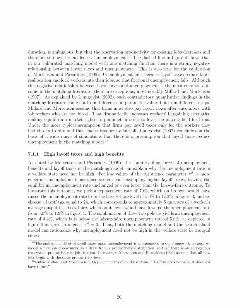
duration, is ambiguous, but that the reservation productivity for existing jobs decreases andtherefore so does the incidence of unemployment.14 The dashed line in figure 4 shows thatin our calibrated matching model with one matching function there is a strong negativerelationship between layoff taxes and unemployment. This is also true for the calibrationof Mortensen and Pissarides (1999). Unemployment falls because layoff taxes reduce laborreallocation and lock workers into their jobs, so that frictional unemployment falls. Althoughthis negative relationship between layoff taxes and unemployment is the most common out-come in the matching literature, there are exceptions, most notably Millard and Mortensen(1997). As explained by Ljungqvist (2002), such contradictory quantitative findings in thematching literature come not from differences in parameter values but from different setups.Millard and Mortensen assume that firms must also pay layoff taxes after encounters withjob seekers who are not hired. That dramatically increases workers’ bargaining strengths,making equilibrium market tightness plummet in order to level the playing field for firms.Under the more typical assumption that firms pay layoff taxes only for the workers theyhad chosen to hire and then had subsequently laid off, Ljungqvist (2002) concludes on thebasis of a wide range of simulations that there is a presumption that layoff taxes reduceunemployment in the matching model.15

7.1.1 High layoff taxes and high benefits

As noted by Mortensen and Pissarides (1999), the countervailing forces of unemploymentbenefits and layoff taxes in the matching model can explain why the unemployment rate ina welfare state need not be high. For low values of the turbulence parameter πd, a moregenerous unemployment insurance system can accompany higher layoff taxes, leaving theequilibrium unemployment rate unchanged or even lower than the laissez-faire outcome. Toillustrate this outcome, we pick a replacement rate of 70%, which on its own would haveraised the unemployment rate from the laissez-faire level of 5.0% to 12.3% in figure 3, and wechoose a layoff tax equal to 24, which corresponds to approximately 5 quarters of a worker’saverage output in laissez faire, which on its own would have lowered the unemployment ratefrom 5.0% to 1.9% in figure 4. The combination of these two policies yields an unemploymentrate of 4.4%, which falls below the laissez-faire unemployment rate of 5.0%, as depicted infigure 8 at zero turbulence, πd = 0. Thus, both the matching model and the search-islandmodel can rationalize why unemployment need not be high in the welfare state in tranquiltimes.

14The ambiguous effect of layoff taxes upon unemployment is compounded in our framework because wemodel a new job opportunity as a draw from a productivity distribution, so that there is an endogenousreservation productivity in job creation. In contrast, Mortensen and Pissarides (1999) assume that all newjobs begin with the same productivity level.

15Unlike Millard and Mortensen (1997), our models obey the dictum, “If a firm does not hire, it does nothave to fire.”

20

0 0.2 0.4 0.6 0.8 10

1

2

3

4

5

6

7

8

9

10

Turbulence πd

Une

mpl

oym

ent r

ate

(per

cen

t)

(a) Welfare state

0 0.2 0.4 0.6 0.8 10

1

2

3

4

5

6

7

8

9

10

Turbulence πdU

nem

ploy

men

t rat

e (p

er c

ent)

(b) Laissez-faire economy

Figure 8: (Matching model) Unemployment rates in the welfare state (panel a) and thelaissez-faire economy (panel b). The solid line is total unemployment. The dashed lineshows the unemployed who have suffered skill loss. The policy of the welfare state is (η,Ω) =(0.7, 24).

7.1.2 Turbulence and unemployment

Along with the search-island model, the matching model confirms the finding of Ljungqvistand Sargent (1998, 2007a) that increased turbulence causes unemployment to increase in thewelfare state while it remains virtually unchanged in the laissez-faire economy, as shown infigure 8. As in the search-island model, the positive relationship between turbulence andunemployment is explained by the choices made by laid off workers who have suffered skillloss (dashed line in panel a of figure 8).

Panel a of figure 9 shows that in the welfare state an increase in turbulence increasesthe average duration of unemployment spells but leaves the inflow rate almost unchanged.The higher average duration of unemployment is not shared equally among unemployedworkers. Although all unemployed workers face the same probability of encountering avacancy because they enter a common matching function, job acceptance rates differ amongworkers who are heterogeneous with respect to their skill levels and benefit entitlements.Thus, consider unemployed workers who have been laid off and suffered skill loss. Becauseunemployment benefits are indexed to past earnings, such workers receive benefits that arehigh compared to their current earnings potential. To give up their generous benefits, theseworkers must encounter vacancies with idiosyncratic productivities that are high enoughto induce firms to offer more generous wages. Hence, low-skilled unemployed workers withhigh benefits encounter fewer acceptable matches than do low-skilled unemployed workerswith low benefits. The unchanging inflow rate into unemployment is explained by almost

21

0 0.2 0.4 0.6 0.8 10

1

2

3

4

5

6

Turbulence πd

Inflo

w r

ate

(per

cen

t) a

nd d

urat

ion

(qua

rter

s)

Inflow rate

Duration

(a) Welfare state

0 0.2 0.4 0.6 0.8 10

1

2

3

4

5

6

Turbulence πdIn

flow

rat

e (p

er c

ent)

and

dur

atio

n (q

uart

ers)

Inflow rate

Duration

(b) Laissez-faire economyFigure 9: (Matching model) Inflow rate and average duration of unemployment in the welfarestate (panel a) and the laissez-faire economy (panel b). The dashed line is the averageduration of unemployment in quarters. The solid line depicts the quarterly inflow rate intounemployment as a per cent of the labor force. The policy of the welfare state is given by(η,Ω) = (0.7, 24).

unchanged reservation productivities that determine job destruction. Turning to the laissez-faire economy in panel b of figure 9, both the inflow rate and the average duration ofunemployment are virtually unaffected by turbulence. In the laissez-faire economy, firms andworkers respond to turbulence in ways that leave both the optimal rate of job destructionand the optimal length of time to search for a job unchanged.

Since turbulence sharply increases the average duration of unemployment spells in thewelfare state, after allowing for the equilibrium response in the reservation productivity fornew jobs, one would expect a precipitous fall in market tightness θ = v/u. Thus, the dottedline in figure 10 depicts how market tightness plummets in response to higher turbulence.Alternatively, when varying the level of turbulence, we could have plotted combinations ofstationary equilibrium (u, v) pairs in the space of unemployment and vacancy rates. Such agraph would show that our theory of increased turbulence is consistent with the observationthat the Beveridge curve has shifted outward in Europe since the mid-1970s.16

16In a survey of the matching function, Petrongolo and Pissarides (2001, p. 409) emphasize outward shiftsin the Beveridge curve that “coincide with the secular rise in European unemployment, which started in themid-1970s. The unemployment rate has increased despite the fact that the separation rate and the vacancyrate [both expressed relative to the level of employment] have not shown any trend. The implication forthe matching function is that there are variables beside [unemployment and vacancies] that have played animportant role in matching in the last two decades and these variables contributed to a deterioration of thematching rate.” Our theory of increased turbulence is consistent with this account. The inflow rate intounemployment in panel a of figure 9, which is also the separation rate in our model, is almost unaffected byturbulence in the welfare state. All expressed relative to the level of employment, the separation rate falls

22

To ensure that firms break even when posting vacancies in a more turbulent environment,the invisible hand increases the probability that a vacancy encounters an unemployed worker,and thereby weakens the effective bargaining strength of workers: the lower probability thatan unemployed worker encounters a vacancy causes workers’ outside value to fall. Decreasedwaiting times between matches for vacancies and the associated fall in a worker’s outsidevalue are the invisible hand’s way of improving firms’ prospects in response to two adverseforces on firms’ profits. First and foremost, increased turbulence ignites adverse welfare-state dynamics because, with a given replacement rate, UI becomes more valuable comparedto what can be earned working. This is most apparent in the case of laid off workerswho have suffered skill loss and become low-skilled unemployed workers who are entitled tobenefits that are generous relative to their reduced earnings potential. The invisible handmust compensate firms for meeting such workers, because these encounters are less likelyto result in agreeable matches; and when such matches are formed, wage payments to low-skilled workers who are entitled to high benefits are higher than those to low-skilled workerswho are entitled to low benefits. Second, our representation of turbulence implies a worsetechnology for skill accumulation and, therefore, higher turbulence has detrimental effectson match surpluses in both the welfare state and the laissez-faire economies. The invisiblehand must improve firms’ situations because they have to break even while financing theaverage cost for filling a vacancy out of a fixed fraction of the diminished match surpluses.

Of these two forces that make market tightness fall in response to increased turbulence,that driven by adverse welfare-state dynamics is more important. This assertion emergesfrom the outcome that laissez-faire unemployment in panel b of figure 8 increases onlyslightly in response to increased turbulence: under laissez-faire, the second adverse forcefrom increased turbulence operates, but not the first.

7.2 Multiple matching functions

7.2.1 Separate matching functions for different skills

Figure 10 also reports outcomes of an economy with two separate matching functions forunemployed workers sorted only according to their current skills. It is instructive to comparethe market tightness across the two labor markets in such an economy. When πd = 0,the zero-profit condition for job creation calls for more vacancies per unemployed workerassigned to the low-skill market. Workers with low skills enjoy a higher probability ofencountering a vacancy because there is a larger match surplus to be shared in the caseof a match and therefore more incentive for firms to post vacancies. The larger matchsurplus associated with a low-skilled worker arises from the possibility that employmentmight result in a skill upgrade that leads to a future capital gain for the match. However,the relative advantage for low-skilled unemployed in terms of market tightness erodes quicklyas turbulence increases. When there is turbulence, the low-skill market includes not only

by merely 3%, while the unemployment rate depicted in panel a of figure 8 spans an increase of 128% witha corresponding vacancy rate (not shown) that declines by no more than 14 per cent.

23

0 0.2 0.4 0.6 0.8 10

0.2

0.4

0.6

0.8

1

1.2

1.4

1.6

Mar

ket t

ight

ness

θ

Turbulence πd

Low skills (current)

High skills (current)

# 1

Figure 10: (Matching model) Market tightness θ when there are separate matching functionsfor unemployed based upon their current skills; low skills (solid line) and high skills (dashedline). As a benchmark, the dotted line labeled #1 depicts market tightness in the economywith a single matching function. The government’s policy is given by (η,Ω) = (0.7, 24).

low-skilled workers with low benefits but also laid off workers who have suffered skill lossand are now low-skilled but entitled to high benefits. As discussed above, firms think thatlow-skilled workers who are entitled to high benefits are poor job candidates and, therefore,the invisible hand must compensate firms that post vacancies in the low-skill market byassigning shorter times to encounter an unemployed worker. Thus, there has to be lowermarket tightness and an associated weakening of workers’ effective bargaining strength. Interms of aggregate unemployment, figure 13 shows that the outcome in this economy withtwo matching functions is not much different from the model with a single matching function.

7.2.2 Separate matching functions for different unemployment benefits

In figure 11, we turn to an economy with separate matching functions for unemployed work-ers sorted only according to their benefits. The least desirable job candidates, the low-skilledworkers who are entitled to high benefits, are now pooled with the high-skilled unemployed.When turbulence πd increases, the high-benefit market experiences a precipitous fall in mar-ket tightness, while the decline in the low-benefit market is smaller, at least until turbulencereaches a critical level. When turbulence reaches 0.60, marked by a star in Figure 11, themarket tightness θ = v

uin the high-benefit market has fallen so much that the probability

that a vacancy meets an unemployed worker is equal to one. Higher levels of turbulence fur-ther depress market tightness and reduce the probability that an unemployed worker meetsa vacancy, but the probability that a vacancy meets an unemployed worker remains one.

24

0 0.1 0.2 0.3 0.4 0.5 0.6 0.7 0.8 0.9 10

0.2

0.4

0.6

0.8

1

1.2

1.4

1.6

Mar

ket t

ight

ness

θ

Turbulence πd

Low benefits

High benefits

# 1

Figure 11: (Matching model) Market tightness θ when there are separate matching functionsfor unemployed workers sorted according to their benefits; low benefits (solid line) and highbenefits (dashed line). As a benchmark, the dotted line labeled #1 depicts market tightnessin the economy with a single matching function. The government’s policy is (η,Ω) = (0.7, 24).For πd above .6 denoted by the ∗, the probability that a vacancy meets a worker equals 1.For πd above .96 (the circle), the high benefit market closes.

The short end of the market, the number of vacancies, determines the total number of en-counters. When turbulence reaches another critical level at 0.96 marked by a circle in figure11, market tightness in the high-benefit market has fallen to zero and the market closes. Atlevels of turbulence above this critical point, a firm in the high-benefit market cannot expectto break even by posting a vacancy and meeting a worker with certainty in the next period,even though the worker’s threat point is merely the outside value of remaining unemployedforever. Vacancies in the high-benefit market have become unprofitable because the odds ofencountering a low-skilled worker rather than a high-skilled worker are too high. The pointat which the high-benefit market breaks down obviously depends on the length of a modelperiod. While a shortening of our semiquarterly period would delay and maybe eliminatethe market breakdown, unemployment would still explode when higher turbulence drivesmarket tightness closer to zero. (See footnote 18.)

7.2.3 Comparisons across different pooling arrangements

Figure 13 depicts how aggregate unemployment increases more in response to turbulencein the economy with separate matching functions indexed by unemployed workers’ benefitsthan it does in the economy with a single matching function or in the economy with separatematching functions for unemployed workers sorted according to their current skills. In allthree economies, low-skilled unemployed workers entitled to high benefits harm the prospects

25

of other workers with whom they are pooled within a matching function. However, the impactof these unwanted job candidates is diluted when there is a single matching function in theeconomy or, in the case of multiple matching functions, when these workers are pooled witha group of unemployed workers who can better withstand such a mixing. In our model,the low-skilled workers who are entitled to low benefits are the more resilient group ofunemployed because their match surpluses include the prospects of capital gains associatedwith becoming high-skilled. Hence, low-skilled unemployed workers who are entitled tolow benefits can better bear the burden of being pooled with low-skilled unemployed whoare entitled to high benefits. If these unwanted job candidates are instead pooled withthe least resilient group, namely, high-skilled unemployed workers who are entitled to highbenefits, as when the matching functions are indexed by benefits b but not skills h, aggregateunemployment increases more with turbulence and increases further at the level of turbulencewhere the probability of that a vacancy meets an unemployed worker in the high-benefitmarket has increased to its maximum of one, indicated by a star in figure 13. At higherlevels of turbulence, the ever lower measures of market tightness in figure 11 cause aggregateunemployment virtually to explode in figure 13.17 At the critical level of turbulence indicatedby a circle, the high-benefit market shuts down and unemployment becomes an absorbingstate for all skilled workers who suffer exogenous layoffs. It follows that the solutions toworkers’ and firms’ optimization problems are no longer affected by the incidence of skillloss among the exogenously laid off. Hence, unemployment in figure 13 and measures ofmarket tightness in figure 11 become constant for any turbulence above this critical level.A consequence of the adverse outcomes in the high-benefit market is that market tightnessin the low-benefit market suffers a dramatic decline. The breakdown of the high-benefitmarket is tantamount to a drastic deterioration in the skill accumulation technology. Theargument in section 7.1.2 explains why the invisible hand must lower market tightness in thelow-benefit market to uphold the zero-profit condition for job creation in the face of what islike a deterioration in the economy’s technology.

7.2.4 Three matching functions: sorting according to both skills and benefits

Insights gleaned from the models with two matching functions help to understand the out-comes for the model in which three matching functions sort unemployed workers perfectlyalong all of their attributes. Under our calibration, the labor market for low-skilled workerswho are entitled to high benefits operates only at very low levels of turbulence, and its mar-ket tightness in figure 12 is so low that the probability that a vacancy meets an unemployedworker always equals one. At the critical level of πd = 0.09 indicated by a circle in figure12, the market for low-skilled unemployed workers entitled to high benefits shuts down, justas the high-benefit market did in the economy of subsection 7.2.2. The two active labor

17The unmarked point of inflection at turbulence 0.66 on aggregate unemployment in the economy withseparate matching functions for unemployed workers based upon their benefits in figure 13 coincides with theendogenous job destruction involving high-skilled workers coming to an end. At higher levels of turbulence,high-skilled workers separate from their jobs only because of exogenous job destruction. This equilibriumoutcome somewhat arrests the explosion in unemployment.

26

0 0.2 0.4 0.6 0.8 10

0.2

0.4

0.6

0.8

1

1.2

1.4

1.6

Mar

ket t

ight

ness

θ

Turbulence πd

Low skills/benefits

Low skills and high benefits

High skills/benefits

# 1

Figure 12: (Matching model) Market tightness θ when there are separate matching functionsfor unemployed based upon both their current skills and benefits; low skills/benefits (uppersolid line), high skills/benefits (dashed line) and low skills but high benefits (lower solidline). As a benchmark, the dotted line depicts market tightness in the economy with a singlematching function. The government’s policy is (η,Ω) = (0.7, 24).

markets are characterized by smoothly falling measures of market tightness throughout therange of turbulence in figure 12. This particular outcome resembles the outcome of thesingle matching function model of section 7.1, but here the similarities end. The unem-ployment rate of the model with three matching functions explodes in response to increasedturbulence in figure 13, both before and after the breakdown of the market for low-skilledunemployed entitled to high benefits. This is hardly surprising after the market breakdownbecause unemployment has then become an absorbing state for all workers experiencing skillloss. Hence, the ranks of the unemployed must then inevitably swell in response to higherincidence of skill loss.18

18To examine the effects of a shorter model period, we converted our semiquarterly calibration into a semi-monthly one by rescaling the discount factor, all exogenous transition probabilities, and the multiplicativecoefficient in the matching function so that the laissez-faire outcomes were unchanged. Under the semi-monthly calibration, the corresponding version of figure 13 depicts two lower curves that do not changemuch while the two upper curves are pushed to the right when the shorter model period delays marketbreakdowns until higher levels of turbulence. Specifically, in the economy with three matching functions,there is an interior solution for the probability that a vacancy meets an unemployed worker in the marketfor low-skilled workers with high benefits until turbulence reaches the critical level of 0.23, before whichthe aggregate unemployment rate lies somewhere in between the curve labeled #3 and the other curves infigure 13. But at higher levels of turbulence, the market quickly shuts down with the result that aggregateunemployment reaches the trajectory of the semiquarterly calibration (curve labeled #3 in figure 13).

27

0 0.2 0.4 0.6 0.8 1

20

25

30

35

40

45

50

# 2 (benefits)

# 3

0 0.2 0.4 0.6 0.8 10

2

4

6

8

10

12

14

16

Une

mpl

oym

ent r

ate

for

give

n #

of m

atch

ing

func

tions

Turbulence πd

# 2 (benefits)

# 2 (current skills)

# 1# 3

Figure 13: (Matching model) Aggregate unemployment rates for different number of match-ing functions. The lower solid line depicts the benchmark model with one matching function.The dash-dotted and the upper solid lines refer to the two models with two matching func-tions where the unemployed are sorted by their current skills and their benefits, respectively.The dashed line depicts the model with three matching functions, i.e., the unemployed areperfectly sorted along all of their attributes. The government’s policy is (η,Ω) = (0.7, 24).

28

0 2 4 6 8 10 120

0.05

0.1

0.15

0.2

0.25

0.3

0.35

0.4

0.45

0.5

Haz

ard

rate

of g

aini

ng e

mpl

oym

ent (

sem

iqua

rtel

y)

Time (quarters)

Laissez faire # 1 # 3

Welfare state

# 3

# 1

Figure 14: (Matching model) Semiquarterly hazard rates of gaining employment in turbulenteconomic times, πd = 1.0. The two dashed lines indexed by #1 and #3 depict the welfarestate with one and three matching functions, respectively. The solid line represents thelaissez-faire economy with an almost perfect overlap of the outcomes associated with one andthree matching functions, respectively. The policy of the welfare state is (η,Ω) = (0.7, 24).

7.2.5 Heterogeneity not duration dependence as source of falling hazard rate

Figure 14 depicts the hazard rate of gaining employment in the most turbulent times (πd =1.0). The hazard rate is practically flat in the laissez-faire economy but declines sharply in thewelfare state. The high incidence of long-term unemployment in the welfare state is conveyedgraphically by a hazard rate that is low even at the start of unemployment spells. Comparethis to the much higher and constant hazard rate in the laissez-faire economy. The hazardrate in the welfare state falls with the duration of spells, not because of duration dependence,but because of heterogeneity with respect to skills and benefit entitlements. Our modelallows for no duration dependence in a sense that would allow hazard rates to fall during anunemployment spell for a given unemployed worker. In contrast to Ljungqvist and Sargent(2007a), who assume additional probabilistic skill losses while workers are unemployed andalso probabilistic transitions between age classes, the state vector of an unemployed workerin our matching models is unchanged over the unemployment spell. That implies a constanthazard rate for a given unemployed worker. So the economy-wide hazard rate in figure 14falls with the duration of spells in the welfare state because the least employable workers,those with low but constant hazard rates, constitute an ever larger share of the remainingunemployed at longer spells. These least employable workers are the low-skilled unemployedentitled to high benefits. They have a low but positive hazard rate in the model with onematching function, and a zero hazard rate in the model with three matching functions.

29

8 Alternative views of unemployed European workers

Although they have broadly similar macroeconomic outcomes, our two classes of modelstell different stories about the motivations and experiences of individual European workers.Lucas (1987, p. 56) praised the McCall because “. . . the model’s explicitness invites hardquestioning.” “Questioning a McCall worker is like having a conversation with an out-of-work friend: ‘Maybe you are setting your sights too high’, or ‘Why did you quit your oldjob before you had a new one lined up?’ This is real social science: an attempt to model,to understand , human behavior by visualizing the situation people find themselves in, theoptions they face and the pros and cons as they themselves see them.” A useful way tosummarize differences among the models is to ask how well they remind us, in Lucas’swords, of ‘talking to an unemployed [European] friend’.19 Although an adverse interactionbetween high UI and high turbulence transcends the models, the unemployed workers inthese models have different alibis for why they aren’t working.

8.1 Unemployed Europeans as discouraged workers

Because it emphasizes the factors that influence an unemployed worker’s choice of searchintensity, talking with an unemployed worker in the search-island model most closely re-sembles the conversation that Lucas carried on with an unemployed worker in the McCallmodel. An individual’s search intensity is the only factor that determines his duration ofunemployment. A worker’s search intensity depends on his asset level, his skill level, hisbenefit entitlement, and, as a determinant of the skill accumulation technology, the level ofa parameter πd that governs skill obsolescence at the time of an exogenous job terminationand that we use to measure turbulence. For a given level of turbulence, workers with lowskills, high accumulated financial assets, and high benefit entitlements choose the lowestsearch intensities. The weak incentives to search provided by their high UI entitlements andtheir current low skills are what discourages these ‘discouraged workers’.20

The search-island model has no externalities in the labor market. A worker selling hislabor services or a firm buying those services does not inflict injuries on others in the labormarket beyond what a seller or a buyer of a good ordinarily imposes on competitors. Fur-thermore, since the wage rate is determined competitively in these two models, the holdupproblem that is present in the bargaining setting of the matching model is absent in thesearch-island model. Thus, unemployment in the search-island model directly reflects work-ers’ decisions. After allowing for the time lag imposed by the time-to-create-jobs assumption,firms will create a number of new jobs that is adequate for all workers who are willing towork at the competitive wage and who have ‘found the labor market’ in the search-islandmodel.

19We have added ‘European’ to Lucas’s phrase.20We suspect that properly accounting for the discouraged workers who have taken advantage of the early

retirement and disability programs available in Europe at government expense would turn up even morediscouraged workers than are recorded in the unemployment statistics. See footnote 2.

30

8.2 Unemployed Europeans as victims of congestion and their own

bargaining power

In the matching models, unemployed workers join others who wait in the same matchingfunction, so their employment prospects and their anticipated durations of unemploymentdepend on the characteristics of those other workers. The mixture of skills and UI benefitentitlements of the workers in a pool determine how profitable it is for firms to post vacanciesthere. In a matching function that includes low-skilled workers with different benefits, it ismore costly for firms to match with workers with low skills who are entitled to high UIthan to match with workers with low skills who are entitled to low UI. It requires a higherproductivity draw to form successful matches with the former workers as compared to thelatter workers and for a given productivity draw, bargaining with the former workers leads tohigher wage payments as compared to bargaining with the latter workers. To induce firms topost vacancies in a pool with many low skill, high UI entitlement workers, the invisible handmust set market tightness θ = v/u, the ratio of the pools of job vacancies v and unemployedworkers u, to be low enough that firms can expect to match with workers frequently enough.But this means that workers can expect to match infrequently with firms, so that theirexpected durations of unemployment are high. Thus, if we were to ask an unemployedworker waiting in one of the matching models why he had been unemployed for so long,he could blame the other workers in his matching function whose bad characteristics areresponsible for making market tightness low.

If pressed further about the reasons for his long unemployment spell, a low-skilled un-employed worker with high benefits might concede that his tough bargaining posture during‘job interviews’ might contribute to his current predicament. His high benefits relative tohis current skills give him a high threat point during the Nash bargaining process with anyfuture prospective employer. If we were to ask the worker how he expects to get away withsuch outrageous wage demands when there are so many other unemployed workers also wait-ing in the same matching function, he could point to the fact that a firm will have him as thesole job candidate. If the firm would like to meet other candidates, it would have to expendadditional resources on posting a vacancy and incur a delay of at least one more periodbefore meeting someone else. Besides, any future encounters would also be on a bilateralbasis. A firm could never expect to meet more than one job seeker at the negotiation table.

If the economy consigns low skill, high UI entitlement workers to their own matchingfunction, it is true that unemployment rates for workers not in that ‘skill-losers market’will be lower. But when UI benefits are high and turbulence is high, the existence of suchan isolated market for losers of skills becomes a misfortune for the steady state of theeconomy because high turbulence means that it is the destiny of many workers to passthrough the skill-losers market in which firms optimally post very few vacancies. Hence,the unemployment rate in such an economy virtually explodes when turbulence increasesbecause losers of skills become victims of long-term unemployment in their overly congestedmatching function. Having a single matching function in the economy dilutes the adverseconsequences of high turbulence for unemployment, but even then, by creating more skill

31

losers in the pool of prospective workers, high turbulence in conjunction with high UI causesequilibrium unemployment to grow in order to induce firms to post vacancies.

9 Concluding remarks

9.1 The lynchpin of matching models

Although Petrongolo and Pissarides (2001) call matching functions a “black box,” theycommend them as a tractable device for building labor market frictions into equilibriummacroeconomic models of wages, employment, and unemployment. But as we have seen,seemingly natural modifications of the black box, such as assigning groups of similar workersto their own matching functions, can have dramatic effects on equilibrium outcomes, effectsthat emerge from how the invisible hand adjusts its key signal, the vacancy-unemploymentratio, enough to compensate firms for the cost of posting a vacancy. Our experiments withmultiple matching functions demonstrate how the cost of posting vacancies is the lynchpin,or to use a less kind metaphor, the tail that wags the dog, of matching models.

That the cost of posting vacancies is the lynchpin of matching models is also a mainmessage of recent contributions of Shimer and Hall. Shimer (2005) argues that a standardcalibration of a matching model with a fixed Nash bargaining weight ψ cannot explain thehigh volatility in the vacancy-unemployment ratio (market tightness θ) relative to the lowvolatility in wages that we observe. But Shimer (2005, p. 42) also shows how the twovolatilities can be rationalized under an alternative assumption that specifies that workers’bargaining power ψ changes stochastically (and persistently) over time. Shimer’s calculationshighlight how the economics of recovering a firm’s cost of posting a vacancy is a key partof matching models. Firms must recover their sunk hiring costs by earning returns over aworker’s job tenure. Because a worker’s cumulative output over an average job tenure is somuch greater than the average recruitment cost, with free entry the equilibrium outcomeawards firms only a small fraction of each period’s output. This allows even modest wagefluctuations induced by a stochastic bargaining weight to have large impacts on firms’ smallclaims to output. Therefore, the ‘invisible hand’ must make large adjustments to markettightness in order to sustain profitability in firms’ recruitment efforts.21

While we retain the standard Nash bargaining assumption, firms’ recovery of recruitmentcosts remains the central force in our models with displaced workers who have suffered skillloss and are entitled to generous benefits. Firms fear these workers because their generous

21Hall (2005) seizes on the multitude of wage rules that can be postulated for dividing the match surplusand shows how tampering with assumptions about wage stickiness vastly alters the sensitivity of the matchingmodel to technology shocks. Perhaps to restore discipline to modeling process, Hall (2006) returns to thestandard Nash bargaining assumption but adds the assumption that workers’ bargaining power ψ variesinversely with market tightness. It might seem odd that workers’ bargaining power increases in times ofdifficulties to find jobs. But Hall and Milgrom (2007) explain this outcome by using a bargaining theorythat imparts a limited role to outside options with the rationale that realistic threats are to extend, not toterminate, bargaining.

32

benefits mean that they have to draw high match-specific productivities to employ them,and, even then, only at higher wages than for workers with the same skills but lower bene-fits. In contrast to the empirical literature on matching and heterogeneity that focuses onhow job finding rates depend on individual characteristics, as summarized by Petrongoloand Pissarides (2001), we highlight the theoretical consequences of the externalities thatheterogeneous workers impose on each other and how those externalities depend on work-ers’ groupings into matching functions. Given the evidence about important heterogeneitiesamong the unemployed in Europe, as for example reflected in groups of long-term unem-ployed, we suggest that worker heterogeneity and the appropriate number and grouping ofmatching functions deserve more attention.22

9.2 No externalities in search-island models

Our search-island and matching models have similar labor market outcomes, but the mech-anisms producing them differ. As an illustration, consider figure 3 that shows how theunemployment rate is positively related to the UI replacement rate in the two types of mod-els. The curve for the search-island model is nearly flat for a range of replacement rates below40–50%, while the corresponding curve for the matching model displays a more gradual in-crease. In the matching model, higher benefits affect the unemployment rate by increasingworkers’ threat points for wage bargaining. The invisible hand restores equilibrium after anincrease in the replacement rate by lowering market tightness, thereby causing the proba-bility that a worker encounters a vacancy to fall in order to compensate firms for the lowerexpected returns from posting vacancies that would occur if market tightness were not low-ered. Hence, high benefits make all unemployed workers suffer from increased congestion inthe labor market. This mechanism by which higher benefits lead to higher unemploymentis clearly continuous in the level of benefits. In contrast, the search-island model features adifferent mechanism through which higher benefits raise equilibrium unemployment throughthe response of individual workers’ search behavior. Higher benefits make it less costly toremain unemployed. In response, unemployed workers find it optimal to reduce their searchintensities and so lessen the disutility of searching for a new job. But as seen in figure 3,this effect becomes quantitatively important only at relatively high replacement rates. Thereason is that unemployed workers must fend for themselves. Low replacement rates are oflittle comfort to unemployed workers who must finance their consumption with these lowbenefits and their savings, so their search intensities are not much affected and unemployedworkers concentrate instead on restoring their relatively higher labor market earnings. Butat higher replacement rates, this mechanism for generating unemployment in the search-

22See footnote 11. An early illustration of the tensions inherit in matching models with heterogeneity isPissarides’ (1992) analysis of skill accumulation in a two-period overlapping generations model with a singlematching function. His focus is on how the externality in the matching process gives rise to a propagationmechanism in which a temporary shock to employment can persist for a long time. Hornstein et al. (2003) usea matching model with one matching function, workers with one skill level, but physical capital of differentvintages, as a tool for studying how different rates of embodied technical change impinge on equilibriumoutcomes, including wage distributions.

33

island model becomes very potent and workers choose to furlough themselves into drawn outunemployment spells by setting low search intensities.

9.3 Responsibility for being unemployed

In a matching model, an unemployed worker can legitimately shift much of the blame for hissituation to the adverse congestion effects induced by the behavior of the other workers andthe firms with whom he waits in a matching function. In a search model, the responsibilityfor being unemployed falls squarely on an unemployed individual. Luck plays a role inthe search process, but an unemployed worker cannot blame congestion externalities for hispredicament, so he can’t blame the behavior of firms or other unemployed workers. In oursearch-island model, an unemployed worker masters his own destiny by choosing his or hersearch intensity23 and in equilibrium the economy creates as many jobs as workers are willingto find. Blanchard (2006, p. 24) provides an empirical observation that is consistent withthis benign view of job creation: “even in economies with high unemployment, exogenousmovements in the labor force – due to demography or repatriation, such as the return ofEuropean nationals after the independence of former colonies – translate fairly quickly intomovements in employment.”

23In the search model of Ljungqvist and Sargent (2007a), an unemployed worker also chooses a reservationwage.

34

Appendices

Two appendices describe the models in enough detail to allow a reader to prepare com-puter programs to compute equilibria.

A Search-island model

A.1 Firm’s problem

The Bellman equations of an existing firm are

V f (h, z) = max

V f (h, z) ,−Ω

, (10)

V f (h, z) = maxk

zkα (1 + h)1−α − w (1 + h) − (i+ δ) k

+1 − ρ

1 + i

[

−πoΩ + (1 − πo)∑

h′,z′

pn(h, h′)V f (h′, z′)Q (z, z′)

]

. (11)

The first-order condition for capital in problem (11) is

zαkα−1 (1 + h)1−α = (i+ δ) , (12)

which can be solved for k to obtain the firm’s policy function for choosing capital,

k (h, z) =

[

z α

i+ δ

]1

1−α

(1 + h) . (13)

Associated with the solution to an existing firm’s optimization problem is a reservationproductivity z(h) that satisfies

V f (h, z(h)) = −Ω. (14)

Define the following indicator function

Λ (h, z) =

1, if z ≥ z(h);0, otherwise.

(15)

The break-even condition for starting a new firm is

µ =1

1 + i

∑

z

max

(1 − φ)V f (0, z) + φV f (H, z) , 0

Qo(z) , (16)

where µ is the start-up cost and φ is the fraction of high-skilled workers among all new hires.The maximization in (16) implies a reservation productivity zo that determines whether anew firm hires a worker after it observes its productivity level. The reservation productivitysatisfies

(1 − φ)V f (0, zo) + φV f (H, zo) = 0. (17)

35

Define the following indicator function

Λo(z) =

1, if z ≥ zo;0, otherwise.

(18)

The productivity distribution of new firms that hire workers is

Γ(z) =Λo(z)Qo(z)

∑

z′ Λo(z′)Qo(z′)

. (19)

A.2 Household’s problem

We define three value functions V n(a, h, z), V u(a, h, b), and V r(a) for an employed worker, anunemployed worker, and a retired worker, respectively. The state variables are last period’sassets (a), skill index (h), the firm’s current productivity level if employed (z), and theworker’s benefit entitlement if unemployed (b). The benefit entitlement is determined by theworker’s last earnings, which we index by b ∈ 0, H, his skill index when he last worked.Both newborn unemployed workers and laid off unskilled workers have a benefit entitlementindicated by index b = 0.

The Bellman equation of an employed worker is

V n(a, h, z) = maxc,a′

[

log c+ βρV r(a′) + β(1 − ρ)

(

πo∑

h′

po (h, h′)V u(a′, h′, h)

+(1 − πo)∑

h′,z′

pn(h, h′)

V n(a′, h′, z′) Λ (h′, z′)

+V u(a′, h′, h) [1 − Λ (h′, z′)]

Q (z, z′)

)]

(20)

subject to

c+ a′ ≤ (1 + i) a+ (1 − τ) (1 + h)w ,

c, a′ ≥ 0 .

Policy functions cn(a, h, z) and an(a, h, z) give the employed worker’s optimal levels of con-sumption and savings, respectively.

The Bellman equation of an unemployed worker is

V u(a, h, b) = maxc,a′,s

[

log c+ A(1 − s)γ − 1

γ+ βρV r(a′) + β(1 − ρ)

·

(

(

1 − sξ)

V u(a′, h, b) + sξ∑

z′

V n(a′, h, z′) Γ (z′)

)]

(21)

subject to

c+ a′ ≤ (1 + i) a+ (1 − τ)η (1 + b)w ,

c, a′ ≥ 0 , s ∈ [0, 1).

36

Policy functions cu(a, h, b), au(a, h, b), and s (a, h, b) give the unemployed worker’s optimallevels of consumption, savings, and search effort, respectively.

The Bellman equation of a retired worker is

V r(a) = maxc,a′

[

log c+ β(1 − σ)V r(a′)]

(22)

subject to

c+ a′ ≤ (1 + i) a ,

c, a′ ≥ 0 .

Policy functions, cr(a) and ar(a), give optimal consumption and savings, respectively.

A.3 Steady state

In a steady state, a time-invariant measure N (h, z) describes the number of firms operatingwith workers of skill index h ∈ 0, H and productivity level z. This measure must beconsistent with the stochastic process for idiosyncratic shocks and the employment decisionsof firms. If v is the number of newly created firms, then N (· , ·) must satisfy

N (0, z′) = vQo(z′)Λo(z′)(1 − φ) + (1 − ρ)(1 − πo)Λ(0, z′)

·∑

h,z

pn(h, 0)N(h, z)Q(z, z′), (23)

N (H, z′) = vQo(z′)Λo(z′)φ+ (1 − ρ)(1 − πo)Λ(H, z′)

·∑

h,z

pn(h,H)N(h, z)Q(z, z′). (24)

Time-invariant measures yn(a, h, z), yu(a, h, b), and yr(a), respectively, describe the num-bers of employed, unemployed, and retired households with various individual characteristics.These measures are implied by the optimal decision rules by firms and households:

yn(a′, h′, z′) = (1 − ρ)

[

(1 − πo)Λ (h′, z′)∑

a,h,z:an(a,h,z)=a′

pn(h, h′) yn(a, h, z)Q (z, z′)

+Γ (z′)∑

a,b:au(a,h′,b)=a′

s(a, h′, b)ξ yu(a, h′, b)

]

; (25)

yu(a′, h, b) = (1 − ρ)

πo∑

a,z:an(a,b,z)=a′

po(b, h) yn(a, b, z)

+(1 − πo)∑

a,z,z′:an(a,b,z)=a′

pn(b, h) yn(a, b, z)[

1 − Λ (h, z′)]

Q (z, z′)

37

+∑

a:au(a,h,b)=a′

yu(a, h, b)[

1 − s (a, h, b)ξ]

+I(h, b)σ∑

a:ar(a)=a′

yr(a) , (26)

yr(a′) = (1 − σ)∑

a:ar(a)=a′

yr(a)

+ρ

[

∑

a,h,z:an(a,h,z)=a′

yn(a, h, z) +∑

a,h,b:au(a,h,b)=a′

yu(a, h, b)

]

, (27)

where I(h, b) is an indicator function that equals one if h = b = 0 and zero otherwise.Following Alvarez and Veracierto (2001),we consider steady-state equilibria without pub-

lic debt. The government balances its budget every period, implying

0 = τ w∑

h,z

(1 + h)N (h, z) + ΩD − (1 − τ)η w∑

a,h,b

(1 + b)yu(a, h, b) , (28)

where the amount of job destruction D is

D = (1−ρ)

πo∑

h,z

N (h, z)+(1−πo)∑

h,h′,z,z′

pn(h, h′)[

1−Λ (h′, z′)]

N (h, z)Q (z, z′)

. (29)

The market-clearing condition in the goods market is

c+ δk + µv =∑

h,z

N(h, z) z k(h, z)α(1 + h)1−α, (30)

where aggregate consumption and the aggregate capital stock, respectively, are

c =∑

a,h,z

cn(a, h, z) yn(a, h, z) +∑

a,h,b

cu(a, h, b) yu(a, h, b) +∑

a

cr(a) yr(a) , (31)

k =∑

h,z

N(h, z) k(h, z). (32)

There are two equilibrium conditions in the labor market. First, the measure of newfirms that hire workers, v

∑

z Λo(z)Qo(z), must equal the measure of unemployed workerswho accept employment. Second, the skill ratio φ among new hires that the firm takes asexogenous must equal the equilibrium skill ratio among new hires. We can use the time-

38

invariant population measures to express these equilibrium conditions as:

v =

(1 − ρ)∑

a,h,b

s(a, h, b)ξ yu(a, h, b)

∑

z

Λo(z)Qo(z), (33)

φ =

∑

a,b

s(a,H, b)ξ yu(a,H, b)

∑

a,h,b

s(a, h, b)ξ yu(a, h, b). (34)

Households’ aggregate demand for assets

a =∑

a,h,z

a yn(a, h, z) +∑

a,h,b

a yu(a, h, b) +∑

a

a yr(a) , (35)

should equal the supply of assets, which consists of the aggregate capital stock k and thevalue of claims to the economy’s firms:

a = k +

∑

h,z

[

z k(h, z)α(1 + h)1−α − w(1 + h) − (i+ δ)k(h, z)]

N(h, z) − µv − ΩD

i. (36)

B Matching models

B.1 Single matching function

When there is a single matching function, the probability that a firm meets a worker withskill h and benefit entitlement b is

λf (h, b) =M(v, u)

v

u(h, b)

u= m(θ)

u(h, b)

v(37)

and the probability that a worker with skill h and benefit entitlement b is matched with avacancy is

λw(h, b) =M(v, u)

u= m(θ), (38)

which is independent of (h, b). When we introduce multiple matching functions in subsectionB.5, the probability that a worker with skill h and benefit entitlement b is matched with avacancy will depend on (h, b).

39

B.2 Match surplus

When an unemployed worker with skill h and benefit entitlement b meets a firm with avacancy, the firm-worker pair draws productivity z from a distribution Qo

h(z). The firm andthe worker will stay together and produce if the match surplus So(h, z, b) is positive:

So(h, z, b) = max

(1 − τ)z − [1 − β(1 − ρ)]W (h, b)

+β(1 − ρ)

[

−πoΩ + (1 − πo)∑

h′,z′

pn(h, h′)Qh′(z, z′)S(h′, z′)

]

, 0

, (39)

where W (h, b) is the worker’s outside value, and S(h, z) is the surplus associated with acontinuing match. A worker with skill h and benefit entitlement b has an outside optionwith value

W (h, b) = b(b) + β(1 − ρ)

[

W (h, b) + λw(h, b)∑

z

ψSo(h, z, b)Qoh(z)

]

. (40)

Free entry makes the firm’s outside value zero. The firm and worker split the match surplusSo(h, z, b) through Nash bargaining, with outside values as threat points. Let ψ ∈ (0, 1)denote the worker’s share of the match surplus. Because both parties want a positive matchsurplus, there is mutual agreement on whether to form a match. The reservation productivityzo(h, b) satisfies

So(h, zo(h, b), b) = 0. (41)

The surplus of a continuing match is

S(h, z) = max

(1 − τ)z − [1 − β(1 − ρ)]W (h, h)

+β(1 − ρ)

[

−πoΩ + (1 − πo)∑

h′,z′

pn(h, h′)Qh′(z, z′)S(h′, z′)

]

, −Ω

. (42)

The government’s policy of imposing a layoff tax Ω on matches that break makes (42) differfrom expression (39).24 A reservation productivity z(h) satisfying

S (h, z(h)) = −Ω (43)

characterizes whether a match is dissolved.

B.3 Zero-profit condition

In equilibrium, firms expect to break even when posting a vacancy:

µ = β(1 − ψ)∑

h,z,b

λf (h, b)So(h, z, b)Qoh(z). (44)

This condition will pin down the equilibrium value of market tightness θ.

24Another difference between expressions (39) and (42) is that an employed worker’s benefit entitlementis encoded in his skill level h, so there is one less state variable in surplus expression (42).

40

B.4 Wage determination

Alternative wage structures support the same equilibrium allocation. We follow Mortensenand Pissarides (1999) and assume a two-tier wage system.25 In particular, when a firm witha vacancy meets an unemployed worker with skill h and benefit entitlement b, they bargain.The worker’s outside value is W (h, b) and the firm’s outside value is zero. Because they donot incur the layoff tax if they do not reach an agreement, the layoff tax does not directlyaffect the bargaining between a newly matched worker and firm. But if they succeed informing a match, the firm must pay the layoff tax after any future breakup. We capture thisby setting the firm’s threat point equal to −Ω in future Nash bargaining.

These assumptions give rise to a two-tier wage system. There is one wage functionwo(h, z, b) for the initial round of negotiations between a newly matched firm and worker,and another wage function w(h, z) associated with renegotiations in an ongoing match. Thesewage functions satisfy

wo(h, z, b) = W (h, b) + ψSo(h, z, b) − β(1 − ρ)

πo∑

h′

po(h, h′)W (h′, h)

+(1 − πo)∑

h′,z′

pn(h, h′)Qh′(z, z′)(

ψ[

S(h′, z′) + Ω]

+W (h′, h′))

, (45)

w(h, z) = W (h, h) + ψ[

S(h, z) + Ω]

− β(1 − ρ)

πo∑

h′

po(h, h′)W (h′, h)

+(1 − πo)∑

h′,z′

pn(h, h′)Qh′(z, z′)(

ψ[

S(h′, z′) + Ω]

+W (h′, h′))

. (46)

B.5 Multiple matching functions

We entertain some alternative specifications that proliferate matching functions in the spiritof Mortensen and Pissarides (1999), who postulated that workers with different skill levelsget matched with vacancies in separate but identical matching functions with market-specificinputs of unemployment and vacancies. We must modify their specification because theyassumed that workers are permanently endowed with a particular skill level, and we don’t.We consider three alternative specifications:

1. Separate matching functions for unemployed workers with different skill levels, yieldingdifferent equilibrium vacancies v(h) for h ∈ 0, H.

25The risk neutral firm and worker would be indifferent between adhering to this two-tier wage system orone in which workers receive a fraction ψ of the match surplus S(h, z) in every period (which would havethe worker paying a share ψ of any future layoff tax). As emphasized by Ljungqvist (2002), the wage profile,not the allocation, is affected by the two-tier wage system. Optimal reservation productivities remain thesame. Under the two-tier wage system, a newly hired worker in effect posts a bond that equals his share ofthe future layoff tax.

41

2. Separate matching functions for unemployed workers having different benefit entitle-ments, yielding different equilibrium vacancies v(b) for each b ∈ 0, H.

3. Separate matching functions for unemployed workers indexed by both their currentskill h and their skill b in their last employment, yielding equilibrium vacancies v(h, b)for each pair of values (h, b) ∈ 0, H × 0, H.

With a slight abuse of notation, for all three specifications, we use the function v(j) to denotevacancies in market j, where j = h in the first specification, j = b in the second one, andj = (h, b) in the third one. Similarly, for all three specifications, we let θ(j) denote markettightness in market j which is equal to

θ(j) =v(j)

∑

(h, b)∈Υ(j)

u(h, b), (47)

where the summation set Υ(j) depends on the specification: Υ(h) = (h, 0), (h,H) in thefirst one, Υ(b) = (0, b), (H, b) in the second one, and Υ(h, b) = (h, b) in the third one.The corresponding probabilities that an unemployed worker finds a vacancy and that a firmwith a vacancy finds a worker, respectively, equal

λw(h, b)

∣

∣

∣

∣

∣

(h, b)∈Υ(j)

=

M

(

v(j),∑

(h, b)∈Υ(j)

u(h, b)

)

∑

(h, b)∈Υ(j)

u(h, b)= m(θ(j)) , (48)

λf (h, b)

∣

∣

∣

∣

∣

(h, b)∈Υ(j)

=

M

(

v(j),∑

(h, b)∈Υ(j)

u(h, b)

)

v(j)

u(h, b)∑

(h, b)∈Υ(j)

u(h, b)= m(θ(j))

u(h, b)

v(j). (49)

The zero-profit condition for posting a vacancy in market j is

µ = β(1 − ψ)∑

(h, b)∈Υ(j); z

λf (h, b)So(h, z, b)Qo

h(z), (50)

where µ is the cost of posting a vacancy, and match surpluses are determined as describedin section B.2. Wage determination is also the same as in section B.4.

42

References

Alonso-Borrego, Cesar, Jesus Fernandez-Villaverde, and Jose E. Galdon-Sanchez. 2004. Eval-uating Labor Market Reforms: A General Equilibrium Approach. Unpublished.

Alvarez, Fernando and Marcelo Veracierto. 2001. Severance Payments in an Economy withFrictions. Journal of Monetary Economics 47:477–498.

Blanchard, Olivier. 2006. European Unemployment: The Evolution of Facts and Ideas.Economic Policy 21:5–59.

Davis, Steven. 1995. The Quality Distribution of Jobs and the Structure of Wages in SearchEquilibrium. NBER Working Paper 8434.

DenHaan, Wouter, Christian Haefke, and Garey Ramey. 2001. Shocks and Institutions in aJob Matching Model. NBER Working Paper 8463.

Diamond, Peter A. 1982. Wage Determination and Efficiency in Search Equilibrium. Review

of Economic Studies 49:217–227.

Farber, Henry. 1997. The Changing Face of Job Loss in the United States, 1981-1995.Brookings Papers on Economic Activity: Microeconomics 55–128.

———. 2005. What Do We Know about Job Loss in the United States? Evidence fromthe Displaced Workers Survey, 1984-2004. Federal Reserve Bank of Chicago Economic

Perspectives 29(2):13–28.

Gottschalk, Peter and Robert Moffitt. 1994. The Growth of Earnings Instability in the U.S.Labor Market. Brookings Papers on Economic Activity (2):217–272.

Hall, Robert E. 2005. Employment Fluctuations with Equilibrium Wage Stickiness. American

Economic Review 95:50–65.

———. 2006. Sources and Mechanisms of Cyclical Fluctuations in the Labor Market. Stan-ford University.

Hall, Robert E. and Paul R. Milgrom. 2007. The Limited Influence of Unemployment on theWage Bargain. Stanford University.

Heckman, James J. 2003. Flexibility, Job Creation and Economic Performance. CESifo

Forum 4(2):29–32.

Hornstein, Andreas, Per Krusell, and Giovanni L. Violante. 2003. Vintage Capital as anOrigin of Inequalities. Unpublished.

Hosios, Arthur J. 1990. On the Efficiency of Matching and Related Models of Search andUnemployment. Review of Economic Studies 57:279–298.

43

Jacobson, Louis S., Robert J. LaLonde, and Daniel G. Sullivan. 1993. Earnings Losses ofDisplaced Workers. American Economic Review 83:685–709.

Kambourov, Gueorgui and Iourii Manovskii. 2005. Rising Occupational and Industry Mobil-ity in the United States: 1968–1997. University of Toronto and University of Pennsylvania.

Katz, Lawrence F. and David H. Autor. 1999. Changes in the Wage Structure and EarningsInequality. In Handbook of Labor Economics, Vol. 3A, edited by Orley Ashenfelter andDavid Card. Amsterdam: Elsevier.

Krugman, Paul R. 1987. Slow Growth in Europe: Conceptual Issues. In Barriers to European

Growth: A Transatlantic View, edited by Robert Z. Lawrence and Charles L. Schultze.Washington, D.C.: Brookings Institution.

Layard, Richard, Stephen Nickell, and Richard Jackman. 1991. Unemployment: Macroeco-

nomic Performance and the Labour Market. Oxford: Oxford University Press.

Ljungqvist, Lars. 2002. How Do Layoff Costs Affect Employment? Economic Journal

112:829–853.

Ljungqvist, Lars and Thomas J. Sargent. 1998. The European Unemployment Dilemma.Journal of Political Economy 106:514.

———. 2004. European Unemployment and Turbulence Revisited in a Matching Model.Journal of the European Economic Association 2:456–468.

———. 2007a. Two Questions about European Unemployment. Forthcoming in Economet-

rica.

———. 2007b. Understanding European Unemployment with a Representative FamilyModel. Departments of Economics, Stockholm School of Economics and New York Uni-versity.

Lucas, Robert E., Jr. 1987. Models of Business Cycles. Oxford and New York: BasilBlackwell.

Lucas, Robert E., Jr. and Edward C. Prescott. 1974. Equilibrium Search and Unemployment.Journal of Economic Theory 7:188–209.

Millard, Stephen P. and Dale T. Mortensen. 1997. The Unemployment and Welfare Effectsof Labor Market Policy: A Comparison of the USA and the UK. In Unemployment Policy:

Government Options for the Labor Market, edited by Dennis Snower and Guillermo de laDehesa. Cambridge, UK: Cambridge University Press.

Mortensen, Dale T. 1982. Property Rights and Efficiency in Mating, Racing, and RelatedGames. American Economic Review 72:968–979.

44

Mortensen, Dale T. and Christopher A. Pissarides. 1999. Unemployment Responses to ‘Skill-Biased’ Technology Shocks: The Role of Labor Market Policy. Economic Journal 109:242–265.

OECD. 2003. Employment Outlook. Paris.

Petrongolo, Barbara and Christopher A. Pissarides. 2001. Looking into the Black Box: ASurvey of the Matching Function. Journal of Economic Literature 39 (2):390–431.

Pissarides, Christopher A. 1992. Loss of Skill During Unemployment and the Persistence ofEmployment Shocks. Quarterly Journal of Economics 107:1371–1391.

———. 2000. Equilibrium Unemployment Theory. Cambridge, Massachusetts: MIT Press,second ed.

Shimer, Robert. 2005. The Cyclical Behavior of Equilibrium Unemployment and Vacancies.American Economic Review 95:25–49.

45