Is Unemployment Helpful in Understanding Inflation?

Is Unemployment Helpful in Understanding Inflation?

By Taeyoung Doh

Price stability is one of the main objectives of Federal Reserve monetary policy. To achieve this objective, the Federal Reserve employs forecasts of inflation. These forecasts help policymakers

determine the appropriate stance of monetary policy.Economic slack is one of the most widely used short-term pre-

dictors for inflation. Economic slack is a measure of underutilized re-sources in the economy, such as labor and capital. A large amount of economic slack is commonly thought to exert downward pressure on inflation. For example, the Federal Open Market Committee (FOMC) explicitly mentioned “increasing economic slack” in its March 2009 meeting as a basis for the outlook that “inflation will remain subdued.” This outlook for inflation, along with the elevated unemployment rate, was an important element in the FOMC’s decision to increase mon-etary accommodation through purchases of long-term Treasuries and an expansion of agency Mortage Backed Securities (MBS) purchases.

Economists describe the short-term relationship between econom-ic slack and inflation with the Phillips curve. Using unemployment as a measure of economic slack, the Phillips curve relates the cyclical

Taeyoung Doh is an economist at the Federal Reserve Bank of Kansas City. Carter Braxton, a research associate at the bank, helped prepare the article. This article is on the bank’s website at www.KansasCityFed.org.

5

6 FEDERAL RESERVE BANK OF KANSAS CITY

components of the unemployment rate and inflation. The cyclical component is the difference between the observed level and the av-erage level or underlying trend. According to the Phillips curve, an increase in the cyclical component of the unemployment rate typically exerts downward pressure on the cyclical component of inflation.

The relationship between inflation and unemployment appears to have changed over time. In particular, evidence suggests that the rela-tionship between unemployment and inflation weakened after 1984 as stable inflation expectations played a more significant role in inflation dynamics. However, recent research suggests that the Phillips curve relationship remains intact during economic downturns, including the recent recession.

This article investigates the relationship between cyclical fluctua-tions in inflation and unemployment using a flexible statistical frame-work that adjusts for changes in underlying trends in inflation and unemployment. The empirical results indicate that the relationship between the cyclical components of unemployment and inflation is stronger and more significant during recessions and early in recoveries than during mature expansions. Empirical results also suggest that the trend component of unemployment increases more in a weak recovery than a rapid recovery, resulting in less downward pressure on inflation. Hence, carefully assessing the size of the cyclical component of unem-ployment is important for understanding inflation dynamics.

The first section reviews the literature on the short-term empirical relationship between unemployment and inflation. The second section explains the statistical framework and estimates the relationship be-tween inflation and unemployment using this flexible framework. The third section considers the implications of these results for inflation in the current recovery.

I. THE SHORT-TERM RELATIONSHIP BETWEEN INFLATION AND UNEMPLOYMENT

The Phillips curve relationship has been defined in various ways. The early literature linked the levels of inflation and unemployment (Samuelson and Solow). The modern literature uses a “gap specifica-tion” in which the deviation of inflation from its average level, or trend, is related to the deviation of the current unemployment rate from the

ECONOMIC REVIEW • FOURTH QUARTER 2011 7

nonaccelerating inflation rate of unemployment (NAIRU).1 Underly-ing this gap specification is the idea that long-run, or trend, inflation is primarily determined by inflation expectations. Accordingly, research-ers have examined the empirical short-term relationship between infla-tion and unemployment using various gap specifications that abstract from underlying trends.

Studies of the Phillips curve relationship have focused on two sepa-rate but related issues. The first issue is the statistical relevance of the unemployment gap as an explanatory variable for inflation. The sec-ond issue is the predictive power of the unemployment gap for future inflation relative to inflation forecasts based on other macroeconomic variables. While both issues are of interest, this article focuses on the first issue.2

This section examines changes in the Phillips curve relationship over time and across the business cycle. Empirical studies have found that the relationship between cyclical unemployment and cyclical infla-tion weakened after 1984. The Phillips curve relationship has also been found to vary over the business cycle with a stronger and more signifi-cant relationship during recessions than expansions.

Variability over time in the Phillips curve relationship

The relationship between inflation and unemployment appears to have weakened after 1984. A commonly used specification for the Phil-lips curve indicates that the statistically significant negative relationship between the unemployment rate and inflation from 1960 to 1983 be-came statistically insignificant from 1984 to 1999 (Atkeson and Oha-nian). In this specification, trend inflation is assumed to be equal to inflation in the previous period and the NAIRU is assumed constant at 6 percent.3 The relationship was estimated by regressing future changes in inflation on unemployment.

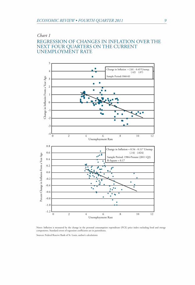
While previous research found that the Phillips curve relationship broke down after 1984, the sample period used in those studies ended in 1999. When the post-1984 period is extended to include the most recent data, however, the relationship becomes significant. In a regres-sion of changes in inflation over the next four quarters on the current unemployment rate using data from 1984 through the second quarter


of 2011, the regression coefficient for unemployment remains negative and statistically significant (Chart 1).4

However, the strength of the Phillips curve relationship remains weaker in the post-1984 period. In the first subsample period from 1960 to 1983, a 1-percent increase in current unemployment is associ-ated with a 0.45-percentage-point decline in inflation over the next four quarters. For the latter period, the same increase in unemployment is associated with only a 0.11-percentage-point decline in inflation over the next four quarters, mitigating the economic significance of the Phil-lips curve relationship.

In an alternative specification, the Phillips curve relationship is found to be similar across subperiods. Specifying trend inflation as a weighted average of past inflation, the regression coefficient on unem-ployment does not change in a statistically significant way across the two subperiods (Stock and Watson 2007).

Variability over the business cycle in the Phillips curve relationship

The relationship between inflation and unemployment is stron-ger during recessions than expansions. In the postwar period, one regularity of disinflationary periods is that they all have occurred during or just following recessions (Stock and Watson 2010). Thus, during recessions since 1960, the unemployment rate has been use-ful for predicting inflation. The rise in unemployment coupled with the substantial decline of inflation during the Great Recession of 2007-09 is another example of this regularity (Liu and Rudebusch).

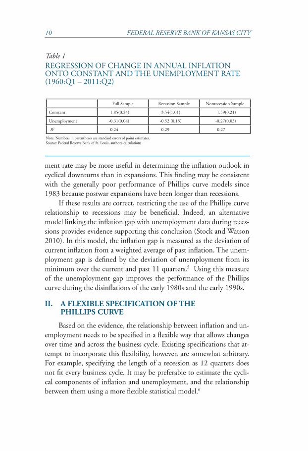
A simple statistical exercise confirms that the relationship be-tween unemployment and inflation has been stronger during reces-sions since 1960. Based on a regression of changes in the annual inflation rate on the unemployment rate, a 1-percent increase in unemployment is associated with a 0.52-percentage-point decline in inflation during recessions (Table 1). For the full sample, a simi-lar increase in unemployment is associated with a 0.31-percentage-point decline in inflation. In addition, changes in unemployment explain a larger percentage of the variation in inflation during reces-sions, as captured by a higher value of the R2 statistic.

This evidence suggests that the strength of the Phillips curve relationship changes over the business cycle. Therefore, the unemploy-


-4

-3

-2

-1

0

1

2

3

4

5

0 2 4 6 8 10 12

Cha

nge

in I

nflat

oin

From

a Y

ear

Ago

Unemployment Rate

Change in Inflation = 2.81 - 0.45*Unemp. (.42) (.07) Sample Period:1960-83

Chart 1 REGRESSION OF CHANGES IN INFLATION OVER THE NEXT FOUR QUARTERS ON THE CURRENT UNEMPLOYMENT RATE

-1.2

-1.0

-0.8

-0.6

-0.4

-0.2

0.0

0.2

0.4

0.6

0.8

0 4 2 6 8 10 12 Unemployment Rate

Perc

ent C

hang

e in

Infla

tion

From

a Y

ear A

go

Change in Inflation = 0.54 - 0.11* Unemp. (.14) (.024)

Sample Period: 1984-Present (2011 Q2)R-Square = 0.17

Notes: Inflation is measured by the change in the personal consumption expenditure (PCE) price index excluding food and energy components. Standard errors of regression coefficients are in parentheses.

Sources: Federal Reserve Bank of St. Louis, author’s calculations


ment rate may be more useful in determining the inflation outlook in cyclical downturns than in expansions. This finding may be consistent with the generally poor performance of Phillips curve models since 1983 because postwar expansions have been longer than recessions.

If these results are correct, restricting the use of the Phillips curve relationship to recessions may be beneficial. Indeed, an alternative model linking the inflation gap with unemployment data during reces-sions provides evidence supporting this conclusion (Stock and Watson 2010). In this model, the inflation gap is measured as the deviation of current inflation from a weighted average of past inflation. The unem-ployment gap is defined by the deviation of unemployment from its minimum over the current and past 11 quarters.5 Using this measure of the unemployment gap improves the performance of the Phillips curve during the disinflations of the early 1980s and the early 1990s.

II. A FLEXIBLE SPECIFICATION OF THE PHILLIPS CURVE

Based on the evidence, the relationship between inflation and un-employment needs to be specified in a flexible way that allows changes over time and across the business cycle. Existing specifications that at-tempt to incorporate this flexibility, however, are somewhat arbitrary. For example, specifying the length of a recession as 12 quarters does not fit every business cycle. It may be preferable to estimate the cycli-cal components of inflation and unemployment, and the relationship between them using a more flexible statistical model.6

Table 1 REGRESSION OF CHANGE IN ANNUAL INFLATION ONTO CONSTANT AND THE UNEMPLOYMENT RATE (1960:Q1 – 2011:Q2)

Note: Numbers in parentheses are standard errors of point estimates.Source: Federal Reserve Bank of St. Louis, author’s calculations

Full Sample Recession Sample Nonrecession Sample

Constant 1.85(0.24) 3.54(1.01) 1.59(0.21)

Unemployment -0.31(0.04) -0.52 (0.15) -0.27(0.03)

R2 0.24 0.29 0.27


This section provides an analysis of the time-varying relationship between the inflation gap and the unemployment gap using a statisti-cal model that separates cyclical components from trend components. The results suggest that the cyclical components of unemployment and inflation, as well as their relationship, vary over time. In line with the previous research, the negative relationship between the unemployment gap and the inflation gap becomes stronger during recessions. However, the implication of this finding for the inflation outlook needs to be bal-anced against the increase in trend unemployment during recessions, which reduces the unemployment gap.

The statistical model

The statistical model consists of three economic variables. The first two variables are intended to capture the Phillips curve relationship: inflation in the core personal consumption expenditures (PCE) price index and the unemployment rate. The third variable is the interest rate on the 10-year Treasury note, which is included to capture movements in trend inflation.7

The model is specified as a vector autoregressive (VAR) process. The sample period is the first quarter of 1960 to the second quarter of 2011. The model follows Cogley and Sargent, except that the 10-year Treasury rate is used instead of the 3-month Treasury rate.8 A detailed description of the model is provided in the Appendix.

Coefficients in the VAR are assumed to vary over time, which allows time variation in the relationships between the three variables as well as in their underlying trends. In addition, the model allows for varia-tion in volatility over time, which is intended to capture changes in macroeconomic conditions over the sample period. In the model, inflation (π

t) is assumed to have a linear relation with two lags of

inflation (πt-1

, πt-2

) unemployment (ut-1

,ut-2

) and the 10-year Treasury rate (i

10,t-1, i10,t-2

).9 In particular, the equation is specified as follows:

π π π= + + + + + + + ∈π− − − − − −a b b c u c u d i d it t t t t t t t t t t t t t t1, 1 2, 2 1, 1 2, 2 1, 10, 1 2, 10, 2 ,

(1)

where at

,bj,t

,cj,t and d

j,t (j=1,2) are coefficients and επ,t is the

residual of the equation.


In this equation, at summarizes the impact of time-varying

trends. To abstract from the change in trends, the relationship can be rewritten in terms of the cyclical, or gap, component of each variable, measured as the deviations of actual levels from trends. Through this adjustment, the impact of time-varying trends is re-moved from the equation and can be expressed as follows:

πgap,t

=b1,t

πgap,t-1

+b2,t

πgap,t-2

+c1,t

ugap,t-1

+c2,t

ugap,t-2

+d1,t

i1gap,10,t-1

+d2,t

igap,10,t-2

+επ,t. (2)

Evidence on the time-varying relationship between the inflation gap and the unemployment gap

The time-varying relationship between the inflation gap and the unemployment gap is estimated by the sum of the coefficients on lagged unemployment (c

1,t+ c

2,t ). This variable captures the overall

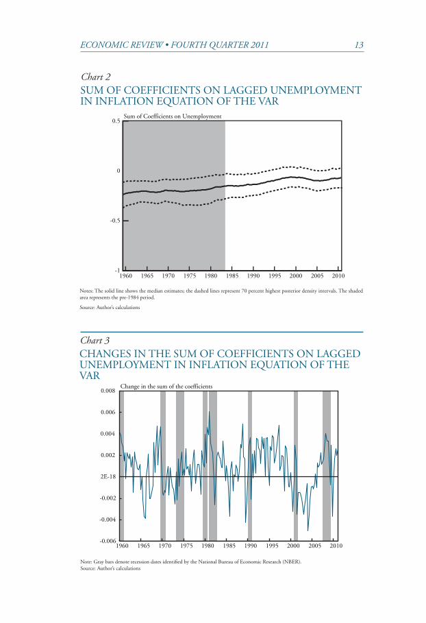
impact of the unemployment rate on inflation. Results show that the sum of the coefficients is much more negative in the period preceding 1984, confirming the findings in the literature on chang-es in the Philips curve relationship over time (Chart 2).

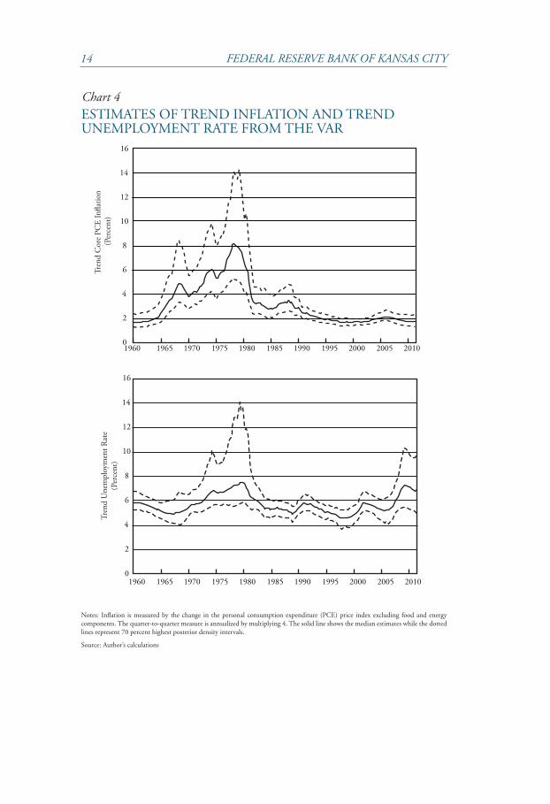
The estimated relationship between the inflation gap and the unemployment gap is cyclical, becoming more negative around re-cessions (Chart 3).10 This finding implies that a given unemploy-ment gap would be associated with a larger change in inflation during recessions than expansions. Furthermore, if trends in unem-ployment and inflation are stable, this suggests a high unemploy-ment rate would exert significant disinflationary pressures during and immediately after recessions.

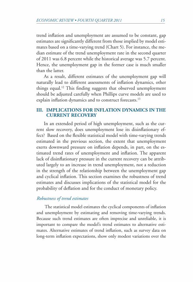
However, time-varying coefficients also imply that trends in unemployment and inflation change over time.11 Based on the esti-mates of the model, substantial time variation is observed for both trend unemployment and trend inflation over the past 50 years (Chart 4). The median estimates of trend inflation have stabilized at a level slightly below 2 percent since the mid-1990s with mini-mal changes during the recent recession. In contrast, trend unem-ployment increased significantly during the 2007-09 recession and remains much higher than the average of trend estimates for the sample period.

Time-varying trends have important implications for the mea-surement of the inflation gap and the unemployment gap. When


Chart 2SUM OF COEFFICIENTS ON LAGGED UNEMPLOYMENT IN INFLATION EQUATION OF THE VAR

Chart 3CHANGES IN THE SUM OF COEFFICIENTS ON LAGGED UNEMPLOYMENT IN INFLATION EQUATION OF THE VAR

-1

-0.5

0

0.5

1960 1965 1970 1975 1980 1985 1990 1995 2000 2005 2010

Sum of Coefficients on Unemployment

Notes: The solid line shows the median estimates; the dashed lines represent 70 percent highest posterior density intervals. The shaded area represents the pre-1984 period.

Source: Author’s calculations

Note: Gray bars denote recession dates identified by the National Bureau of Economic Research (NBER). Source: Author’s calculations

-0.006

-0.004

-0.002

2E-18

0.002

0.004

0.006

0.008

1960 1965 1970 1975 1980 1985 1990 1995 2000 2005 2010

Change in the sum of the coefficients


Chart 4 ESTIMATES OF TREND INFLATION AND TREND UNEMPLOYMENT RATE FROM THE VAR

Notes: Inflation is measured by the change in the personal consumption expenditure (PCE) price index excluding food and energy components. The quarter-to-quarter measure is annualized by multiplying 4. The solid line shows the median estimates while the dotted lines represent 70 percent highest posterior density intervals.


0

2

4

6

8

10

12

14

16

1960 1965 1970 1975 1980 1985 1990 1995 2000 2005 2010

Tren

d C

ore

PCE

Infla

tion

(Per

cent

)

0

2

4

6

8

10

12

14

16

1960 1965 1970 1975 1980 1985 1990 1995 2000 2005 2010

Tren

d U

nem

ploy

men

t Rat

e(P

erce

nt)


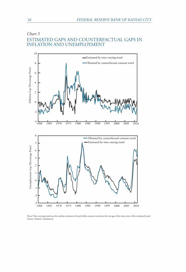
trend inflation and unemployment are assumed to be constant, gap estimates are significantly different from those implied by model esti-mates based on a time-varying trend (Chart 5). For instance, the me-dian estimate of the trend unemployment rate in the second quarter of 2011 was 6.8 percent while the historical average was 5.7 percent. Hence, the unemployment gap in the former case is much smaller than the latter.

As a result, different estimates of the unemployment gap will naturally lead to different assessments of inflation dynamics, other things equal.12 This finding suggests that observed unemployment should be adjusted carefully when Phillips curve models are used to explain inflation dynamics and to construct forecasts.13

III. IMPLICATIONS FOR INFLATION DYNAMICS IN THE CURRENT RECOVERY

In an extended period of high unemployment, such as the cur-rent slow recovery, does unemployment lose its disinflationary ef-fect? Based on the flexible statistical model with time-varying trends estimated in the previous section, the extent that unemployment exerts downward pressure on inflation depends, in part, on the es-timated trend rates of unemployment and inflation. The apparent lack of disinflationary pressure in the current recovery can be attrib-uted largely to an increase in trend unemployment, not a reduction in the strength of the relationship between the unemployment gap and cyclical inflation. This section examines the robustness of trend estimates and discusses implications of the statistical model for the probability of deflation and for the conduct of monetary policy.

Robustness of trend estimates

The statistical model estimates the cyclical components of inflation and unemployment by estimating and removing time-varying trends. Because such trend estimates are often imprecise and unreliable, it is important to compare the model’s trend estimates to alternative esti-mates. Alternative estimates of trend inflation, such as survey data on long-term inflation expectations, show only modest variations over the


Chart 5ESTIMATED GAPS AND COUNTERFACTUAL GAPS IN INFLATION AND UNEMPLOYMENT

Note: Time-varying trend uses the median estimates of trend while constant trend uses the average of the time series of the estimated trend. Source: Author’s calculations

-4

-2

0

2

4

6

8

10

1960 1965 1970 1975 1980 1985 1990 1995 2000 2005 2010

Estimated by time-varying trend

Obtained by counterfactual constant trend

Infla

tion

Gap

(Pe

rcen

tage

Poi

nt)

-3

-2

-1

0

1

2

3

4

5

6

1960 1965 1970 1975 1980 1985 1990 1995 2000 2005 2010

Estimated by time-varying trend

Obtained by counterfactual constant trend

Une

mpl

oym

ent G

ap (

Perc

enta

ge P

oint

)


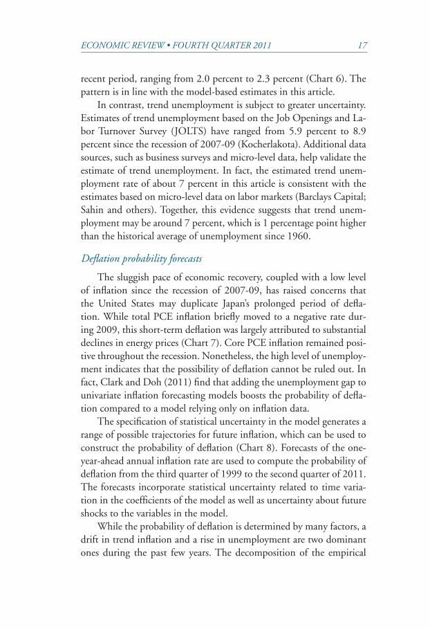
recent period, ranging from 2.0 percent to 2.3 percent (Chart 6). The pattern is in line with the model-based estimates in this article.

In contrast, trend unemployment is subject to greater uncertainty. Estimates of trend unemployment based on the Job Openings and La-bor Turnover Survey (JOLTS) have ranged from 5.9 percent to 8.9 percent since the recession of 2007-09 (Kocherlakota). Additional data sources, such as business surveys and micro-level data, help validate the estimate of trend unemployment. In fact, the estimated trend unem-ployment rate of about 7 percent in this article is consistent with the estimates based on micro-level data on labor markets (Barclays Capital; Sahin and others). Together, this evidence suggests that trend unem-ployment may be around 7 percent, which is 1 percentage point higher than the historical average of unemployment since 1960.

Deflation probability forecasts

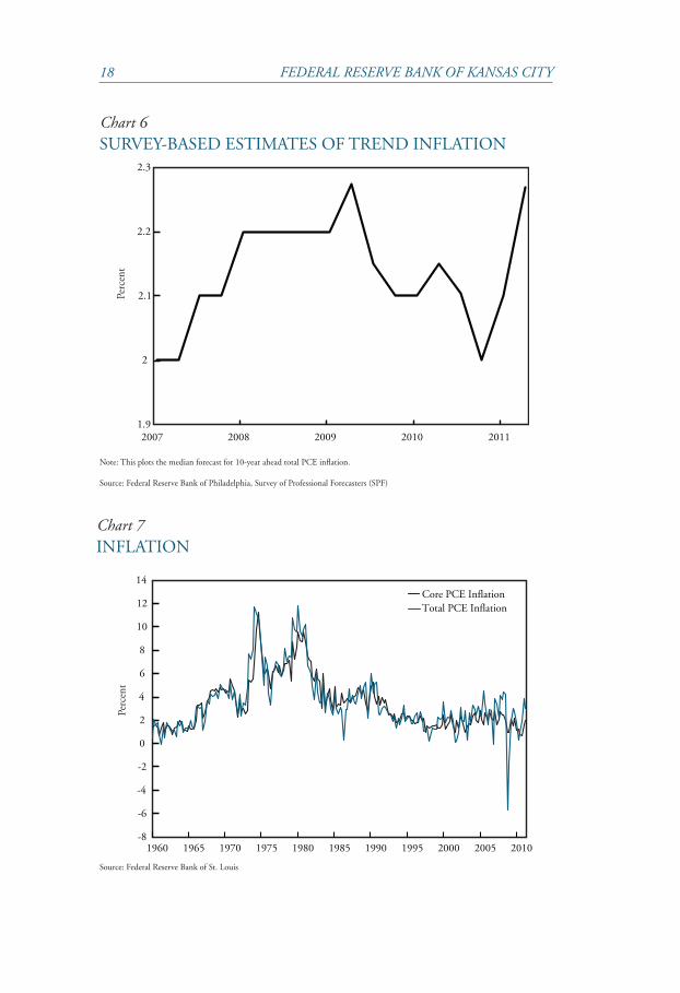
The sluggish pace of economic recovery, coupled with a low level of inflation since the recession of 2007-09, has raised concerns that the United States may duplicate Japan’s prolonged period of defla-tion. While total PCE inflation briefly moved to a negative rate dur-ing 2009, this short-term deflation was largely attributed to substantial declines in energy prices (Chart 7). Core PCE inflation remained posi-tive throughout the recession. Nonetheless, the high level of unemploy-ment indicates that the possibility of deflation cannot be ruled out. In fact, Clark and Doh (2011) find that adding the unemployment gap to univariate inflation forecasting models boosts the probability of defla-tion compared to a model relying only on inflation data.

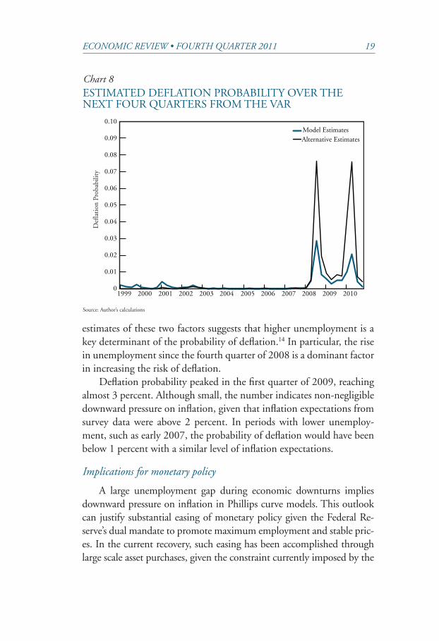
The specification of statistical uncertainty in the model generates a range of possible trajectories for future inflation, which can be used to construct the probability of deflation (Chart 8). Forecasts of the one-year-ahead annual inflation rate are used to compute the probability of deflation from the third quarter of 1999 to the second quarter of 2011. The forecasts incorporate statistical uncertainty related to time varia-tion in the coefficients of the model as well as uncertainty about future shocks to the variables in the model.

While the probability of deflation is determined by many factors, a drift in trend inflation and a rise in unemployment are two dominant ones during the past few years. The decomposition of the empirical


Chart 6SURVEY-BASED ESTIMATES OF TREND INFLATION

Chart 7INFLATION

Note: This plots the median forecast for 10-year ahead total PCE inflation.

Source: Federal Reserve Bank of Philadelphia, Survey of Professional Forecasters (SPF)

Source: Federal Reserve Bank of St. Louis

-8

-6

-4

-2

0

2

4

6

8

10

12

14

1960 1965 1970 1975 1980 1985 1990 1995 2000 2005 2010

Core PCE Inflation Total PCE Inflation

Perc

ent

1.9

2

2.1

2.2

2.3

2007 2008 2009 2010 2011

Percent


estimates of these two factors suggests that higher unemployment is a key determinant of the probability of deflation.14 In particular, the rise in unemployment since the fourth quarter of 2008 is a dominant factor in increasing the risk of deflation.

Deflation probability peaked in the first quarter of 2009, reaching almost 3 percent. Although small, the number indicates non-negligible downward pressure on inflation, given that inflation expectations from survey data were above 2 percent. In periods with lower unemploy-ment, such as early 2007, the probability of deflation would have been below 1 percent with a similar level of inflation expectations.

Implications for monetary policy

A large unemployment gap during economic downturns implies downward pressure on inflation in Phillips curve models. This outlook can justify substantial easing of monetary policy given the Federal Re-serve’s dual mandate to promote maximum employment and stable pric-es. In the current recovery, such easing has been accomplished through large scale asset purchases, given the constraint currently imposed by the

Chart 8ESTIMATED DEFLATION PROBABILITY OVER THE NEXT FOUR QUARTERS FROM THE VAR


0

0.01

0.02

0.03

0.04

0.05

0.06

0.07

0.08

0.09

0.10

1999 2000 2001 2002 2003 2004 2005 2006 2007 2008 2009 2010

Model Estimates Alternative Estimates

Def

lati

on P

roba

bilit

y


zero lower bound on short-term interest rates. The following quote from the FOMC statement on Nov. 3, 2010, illustrates this point.

Currently, the unemployment rate is elevated, and mea-sures of underlying inflation are somewhat low, relative to lev-els that the Committee judges to be consistent, over the longer run, with its dual mandate. Although the Committee antici-pates a gradual return to higher levels of resource utilization in a context of price stability, progress toward its objectives has been disappointingly slow. To promote a stronger pace of economic recovery and to help ensure that inflation, over time, is at levels consistent with its mandate, the Committee decided today to expand its holdings of securities.

This article finds that trend unemployment increases during pe-riods of extended high unemployment, reducing the estimated size of the unemployment gap. As a result, during such periods, the amount of slack in the economy is less than previously estimated. Although the Phillips curve relationship continues to hold, a smaller estimate of the unemployment gap produces less disinflationary pressure.

More broadly, estimates of trend unemployment and trend inflation from the model may provide information on changes in the NAIRU and affect our understanding of future inflation. Incorporating changes in trend unemployment into Phillips curve models may yield better forecasts for policymakers as they seek to provide the proper level of ac-commodation to achieve the Federal Reserve’s dual mandate. Similarly, estimates of changes in trend inflation may provide information on changes in long-term inflation expectations just as surveys of inflation expectations may help provide information about the trend.

IV. CONCLUSIONS

The simultaneous decline of core inflation with the increase of the unemployment rate during the recent recession has renewed the debate regarding the use of indicators of economic slack, such as unemploy-ment, for predicting inflation. Recent studies show that the relation-ship between inflation and unemployment varies over time and tends to be stronger during recessions.


A statistical examination of the time-varying relationship between inflation and unemployment also finds the relationship between the two variables tends to be stronger during recessions. However, this rela-tionship mainly holds for cyclical components of these variables.

Given that trends of inflation and unemployment vary over time, accurate time-varying estimates of the trends of both variables are needed to reliably estimate their cyclical components. In particular, a persistently high unemployment rate is typically accompanied by a ris-ing estimate of trend unemployment, which implies less disinflationary pressure for any given level of the unemployment rate. As a result, a careful adjustment of time-varying trends is necessary when using Phil-lips curve models to assess inflation dynamics.


APPENDIX

This Appendix provides a detailed description of the statistical model and estimation methodology used in this article.

The statistical model

The model closely follows the setup in Cogley and Sargent (2005) but does not allow correlation between innovations in transition equa-tions for time-varying parameters and innovations in measurement equations. The model has the following state space representation.

y x N R

v v N Q

R B H B H H i i d N

, (0, )

, (0, )

,log log . . . (0,1)

t t t t t t

t t t t

t t k t k t k k t

1

1 1, , 1 ,

θθ θ

σ η

= ′ + ∈ ∈= +

= = +−

− −−

In the above equation, yt is a vector of observed variables (the

10-year Treasury note rate, the unemployment rate, and core PCE inflation, in this order), X

t includes a constant and two lags of y

t ,

and θt is a vector of VAR parameters. The VAR parameters evolve as

driftless random walks unless they violate the stationarity condition for the VAR. H

t is a diagonal matrix whose diagonal elements are H

k,t

(k=1,2,3). B is a lower triangular matrix.

Model estimation

Following Cogley and Sargent (2005), the above model is esti-mated using Bayesian methods. Priors of parameters are set based on pre-sample data from the second quarter of 1953 to the fourth quar-ter of 1959. The prior mean and variance of θ0 are determined from the point estimates of the coefficients and their asymptotic variance (P ) in the seemingly unrelated regressions using the pre-sample data. For the prior distribution of Q, an inverse-Wishart distribution with the degree of freedomT

0=22 and a scale matrix T

0* 0.001 *P is used.

The prior distribution of the log of the initial volatility is set to the normal distribution whose mean is equal to the residual variance in the regression using the pre-sample data. The variance of this normal distribution is set to 10. The prior distribution of B is the normal distribution with the zero mean and the covariance matrix equal to the identity matrix multiplied by 10,000. The prior distribution of


the variance of the innovation to volatility process is set to an inverse gamma distribution with the scale parameter equal to 0.0001 and a degree of freedom of 1.

Posterior estimates of parameters are obtained by Markov Chain Monte Carlo (MCMC) methods. One hundred thousand poste-rior draws of parameters are generated and the first 50,000 draws are discarded to reduce the dependence on the starting point of the MCMC chain. Then every 10th draw of the remaining 50,000 draws is used for the posterior inference.


ENDNOTES

1The NAIRU is a baseline rate of unemployment associated with a constant inflation rate. If the unemployment rate is below the NAIRU, inflation tends to rise. If the unemployment rate is above the NAIRU, inflation tends to fall.

2Dotsey, Fujita, and Stark (2011) and Stock and Watson (2009) provide evi-dence for the time-varying forecasting power of Phillips curve models.

3Gordon (1997) shows that an estimate of a time-varying NAIRU has been close to 6 percent since the early 1980s.

4Inflation is measured by the change in the personal consumption expendi-ture (PCE) price index excluding food and energy.

5Stock and Watson (2010) do not take a strong stand on using a three-year rolling window but note that postwar U.S. recessions support such a choice. In a related context, Ball (2009) emphasizes that while a high level of short-term un-employment puts downward pressure on wage inflation, a high level of long-term unemployment does not because the long-term unemployed are more likely to become detached from the labor market.

6Empirical estimates of the NAIRU are typically obtained by isolating the trend component of the observed unemployment rate using various statistical ap-proaches. For example, Gordon (1997) estimates the time-varying NAIRU by a random-walk trend in the observed unemployment rate.

7Economic theory suggests that trend inflation is determined by long-run inflation expectations. A key variable in determining long-term inflation expecta-tions is the central bank’s inflation target (Ireland). Although the Federal Reserve has not adopted a formal target for inflation, the implicit target expected by the public can be obtained from data on interest rates. Because the Federal Reserve typically influences expected inflation through changes in nominal interest rates, adding a nominal interest rate variable to the model may be a useful way to cap-ture the evolution of trend inflation and, therefore, the inflation gap (Cogley and Sargent).

8Since December 2008, the federal funds rate has been at the effective zero lower bound, pushing the 3-month Treasury bill rate also to the effective zero bound. Under these circumstances, the Federal Reserve has been influencing long-term interest rates, using large-scale asset purchases and providing forward guid-ance on the likely future path of the federal funds target rate. The monetary policy report to Congress on March 1, 2011, by the Chairman of the Federal Reserve explicitly mentions that large-scale asset purchases were intended to decrease lon-ger term interest rates. For periods not constrained by the zero lower bound, the 10-year Treasury note rate has a high correlation with both the federal funds rate and the 3-month Treasury bill rate.

9The choice of the lag order of 2 is mainly driven by avoiding the overparam-eterization of the VAR. Clark and Doh (2011) discuss that a higher order does not


improve model fit and forecast performance in an AR model of inflation forecasts with time-varying trend.

10During the 1973-75 and 1980 recessions, the sum of coefficients became less negative. Supply shocks in 1973 (OPEC’s reduction of oil exports) and 1979 (Iranian revolution) might have played a bigger role in these episodes, mitigating the role of the demand side in determining inflation, which is a typical channel of justifying the Phillips curve. And the downward pressure on inflation from high unemployment often comes near the end or immediately after a recession because unemployment is a lagging indicator of economic slack.

11In the statistical model used in this article, trend inflation and trend un-employment can be approximated as the average inflation rate and the average unemployment rate based on current period coefficients in the VAR (Cogley and Sargent). For example, in the following univariate model with time-varying coef-ficients π

t=a

t+b

t π

t-1+∈{π,t}, the trend inflation can be approximated as a

b1t

t−.

12The median estimate of the trend inflation rate in the second quarter of 2011 is 1.8 percent as opposed to the historical average of the trend inflation rate of 3.2 percent. The high trend inflation rate can partially offset the impact of a larger amount of economic slack. Nonetheless, using historical averages generates consistently lower one-year ahead annual inflation forecasts from the second quar-ter of 2008 to the second quarter of 2011.

13The 10-year note rate has a strong positive correlation with inflation, imply-ing that the trend inflation rate comoves with expected inflation embedded in the 10-year note rate. Although lowering the 10-year note rate can increase inflation by decreasing the unemployment rate, quantitatively speaking, that effect is domi-nated by the negative impact on inflation through the expected inflation channel. The relation between the cyclical components of inflation and unemployment is not greatly affected by the 10-year note rate.

14Using notations in equation (1), the current period probability of defla-tion is defined by Prob (∈π,t<–a

t–b

1,tπ

t-1–b

2,tπ

t-2–c

1,tu

t-1– c

2,tu

t-2–d

1,ti10,t-1

–d2,t

i10,t-2

). It turns out that c

1,tu

t-1+c

2,tu

t-2 accounts for the largest share of this probability while

at also has a small role.


REFERENCES

Atkeson, Andrew, and Lee E. Ohanian. 2001. “Are Phillips Curves Useful for Forecasting Inflation?” Federal Reserve Bank of Minneapolis, Quarterly Re-view, vol. 25, no. 1, pp. 2-11.

Ball, Lawrence. 2009. “Is the Phillips Curve Vertical in the Long Run? Hysteresis in Unemployment,” Jeff Fuhrer, Yolanda K. Kodrzycki, Jane Sneddon Little, and Giovanni P. Olivei, eds., Understanding Inflation and the Implications for Monetary Policy: A Phillips Curve Retrospective, The MIT Press.

Barclays Capital. 2011. “Decomposing the Rise in NAIRU” Global Economics Weekly, May.

Clark, Todd E., and Taeyoung Doh. 2011. “A Bayesian Evaluation of Alternative Models of Trend Inflation,” Manuscript, Federal Reserve Bank of Cleveland.

Cogley, Timothy, and Thomas J. Sargent. 2005. “Drifts and Volatilities: Monetary Policies and Outcomes in the post WWII U.S.,” Review of Economic Dynam-ics, April.

Dotsey, Michael. Shigeru Fujita, and Tom Start. 2011 “Do Phillips Curves Con-ditionally Help to Forecast Inflation?” Working Paper, Federal Reserve Bank of Philadelphia.

Hall, Robert E. 2011. “The Long Slump,” American Economic Review, April. Ireland, Peter N. 2007. “Changes in the Federal Reserve’s Inflation Target: Causes

and Consequences,” Journal of Money, Credit, and Banking, December. Kocherlakota, Narayana. 2011. “Labor Markets and Monetary Policy,” speech

given at St. Cloud State University, March 3, available at http://www.min-neapolisfed.org/news_events/pres/index.cfm.

Liu, Zheng, and Glenn Rudebusch. 2010. “Inflation: Mind the Gap,” Federal Reserve Bank of San Francisco, Economic Letter, 2010-02.

Şahin, Ayşegül, Joseph Song, Giorgio Topa, and Giovanni L. Violante. 2011. “Measuring Mismatch in the U.S. Labor Market,” Manuscript, New York University.

Samuelson, P.A., and Robert M. Solow. 1960. “Analytical Aspects of Anti-Infla-tion Policy,” American Economic Review, May.

Stock, James H., and Mark W. Watson. 2007. “Why Has U.S. Inflation Become Harder to Forecast?” Journal of Money, Credit, and Banking, February.

2009. “Phillips Curve Inflation Forecasts,” Jeff Fuhrer, Yolanda K. Kodrzycki, Jane Sneddon Little, and Giovanni P. Olivei, eds., Understanding Inflation and the Implications for Monetary Policy: A Phil-lips Curve Retrospective, The MIT Press.

2010. “Modeling Inflation after the Crisis,” Federal Reserve Bank of Kansas City, Jackson Hole Economic Sym-posium, August.

Documents

Is Unemployment Helpful in Understanding Inflation?