Embed Size (px)
Citation preview
A P T A S T A N D A R D S D E V E L O P M E N T P R O G R A M
RECOMMENDED PRACTICEAmerican Public Transportation Association
1666 K Street NW Washington, DC 20006
APTA SUDS-CC-RP-001-09Approved August 14, 2009
Climate Change Standards Working Group, SUDS Policy and Planning Committee
This Recommended Practice represents a common viewpoint of those parties concerned with its provisions, namely, transit operating/planning agencies, manufacturers, consultants, engineers and general interest groups. The application of any standards, practices or guidelines contained herein is voluntary. In some cases, federal and/or state regulations govern portions of a rail transit system’s operations. In those cases, the government regulations take precedence over this standard. APTA recognizes that for certain applications, the standards or practices, as implemented by individual rail transit agencies, may be either more or less restrictive than those given in this document.
Quantifying Greenhouse Gas Emissions from Transit
Abstract: This Recommended Practice provides guidance to transit agencies for quantifying their greenhouse gas emissions, including both emissions generated by transit and the potential reduction of emissions through efficiency and displacement by laying out a standard methodology for transit agencies to report their greenhouse gas emissions in a transparent, consistent and cost-effective manner.
Keywords: carbon footprinting, climate change, greenhouse gas emission inventory/reporting, mode shift, congestion reduction, land use multiplier
Scope and purpose: This Recommended Practice provides guidance to transit agencies for quantifying their greenhouse gas emissions, including both emissions generated by transit and the potential reduction of emissions through efficiency and displacement. It lays out a standard methodology for transit agencies to report their greenhouse gas emissions in a transparent, consistent and cost-effective manner. It ensures that agencies can provide an accurate public record of their emissions; may help them comply with future state and federal legal requirements; and may help them gain credit for their “early actions” to reduce emissions.
© 2009 American Public Transportation Association
Participants The American Public Transportation Association greatly appreciates the contributions of the following individuals, who provided the primary effort in the drafting of this Recommended Practice.
D.C. Agrawal, New Jersey Transit Justin Antos, AECOM Craig Bilderback, Veolia Transportation Ed Buchanan, Utah Transit Authority William Cowart, Cambridge Systematics Projjal Dutta, NY MTA David Erne, Booz Allen Monica Hale, SAIC Eric Hesse, TriMet Tina Hodges, FTA Cynthia Hoyle, Champaign-Urbana MTD Brian Laverty, Parsons Brinckerhoff Joan LeLacheur, WMATA Cris Liban, Los Angeles MTA Val Menotti, BART Adam Millard-Ball, Stanford University Mark Minor, Chicago RTA Timothy Papandreou, SFMTA Karl Peet, Chicago Transit Authority Gary Prince, King County Metro Steven Silkunas, SEPTA Melanie Simmons, Florida State University Gerry Tumbali, Chicago RTA Jeff Vosler, Central Ohio Transit Authority
Contents 1. Typology of transit greenhouse gas impacts ........................... 1
1.1 Scale ............................................................................................. 2 1.2 Why quantify emissions? ............................................................. 4 1.3 Emission scopes ........................................................................... 4 1.4 Document structure ...................................................................... 5
2. Greenhouse gas emissions from transit .................................. 6 2.1 Operations vs. capital projects ..................................................... 6 2.2 Reporting Scope 1 and 2 emissions (mainly operational) ........... 7 2.3 Reporting Scope 3 emissions (mainly capital) ........................... 18
3. Mode shift to transit ............................................................... 20 3.1 Regional models ........................................................................ 20 3.2 Natural experiments ................................................................... 20 3.3 Calculate mode shift factor ........................................................ 21 3.4 Methodological procedure ......................................................... 22 3.5 Estimating the mode shift factor ................................................ 23
4. Congestion relief .................................................................... 26 4.1 Tier A: Regional Modeling ........................................................ 27 4.2 Tier B: Extrapolating from Urban Mobility Report data ........... 28 4.3 Tier C: Using Urban Mobility Report data ................................ 31
5. The land-use multiplier .......................................................... 32 5.1 What is the land-use multiplier? ................................................ 32 5.2 Evidence for the land-use multiplier .......................................... 33 5.3 Methodological procedure ......................................................... 34 5.4 Caveats and next steps ............................................................... 35
Appendix A: Summary of NTD audit procedures ......................... 36
Appendix B: Description of MTA land-use multiplier methodology 38
References ................................................................................... 42
Definitions .................................................................................... 43
Abbreviations and acronyms ........................................................ 45
APTA-CC-RP-001-09 | Quantifying Greenhouse Gas Emissions from Transit
1
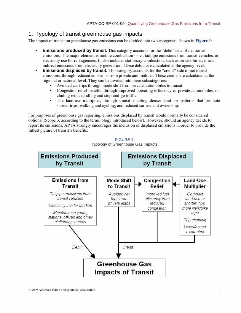
1. Typology of transit greenhouse gas impacts The impact of transit on greenhouse gas emissions can be divided into two categories, shown in Figure 1:
• Emissions produced by transit. This category accounts for the “debit” side of net transit emissions. The major element is mobile combustion—i.e., tailpipe emissions from transit vehicles, or electricity use for rail agencies. It also includes stationary combustion, such as on-site furnaces and indirect emissions from electricity generation. These debits are calculated at the agency level.
• Emissions displaced by transit. This category accounts for the “credit” side of net transit emissions, through reduced emissions from private automobiles. These credits are calculated at the regional or national level. They can be divided into three subcategories:
• Avoided car trips through mode shift from private automobiles to transit. • Congestion relief benefits through improved operating efficiency of private automobiles, in-
cluding reduced idling and stop-and-go traffic. • The land-use multiplier, through transit enabling denser land-use patterns that promote
shorter trips, walking and cycling, and reduced car use and ownership.
For purposes of greenhouse gas reporting, emissions displaced by transit would normally be considered optional (Scope 3, according to the terminology introduced below). However, should an agency decide to report its emissions, APTA strongly encourages the inclusion of displaced emissions in order to provide the fullest picture of transit’s benefits.
FIGURE 1 Typology of Greenhouse Gas Impacts
© 2009 American Public Transportation Association
APTA-CC-RP-001-09 | Quantifying Greenhouse Gas Emissions from Transit
© 2009 American Public Transportation Association 2
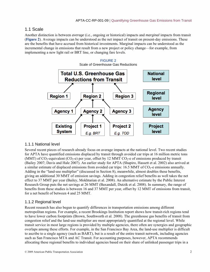
1.1 Scale Another distinction is between average (i.e., ongoing or historical) impacts and marginal impacts from transit (Figure 2). Average impacts can be understood as the net impact of transit on present-day emissions. These are the benefits that have accrued from historical investments. Marginal impacts can be understood as the incremental change in emissions that result from a new project or policy change—for example, from implementing a new light rail or BRT line, or changing fare levels.
FIGURE 2 Scale of Greenhouse Gas Reductions
1.1.1 National level Several recent pieces of research already focus on average impacts at the national level. Two recent studies for APTA have quantified emissions displaced by transit through avoided car trips at 16 million metric tons (MMT) of CO2-equivalent (CO2-e) per year, offset by 12 MMT CO2-e of emissions produced by transit (Bailey 2007; Davis and Hale 2007). An earlier study for APTA (Shapiro, Hassett et al. 2002) also arrived at a similar estimate of displaced emissions from avoided car trips: 16.5 MMT of CO2-e emissions annually. Adding in the “land-use multiplier” (discussed in Section 8), meanwhile, almost doubles these benefits, giving an additional 30 MMT of emission savings. Adding in congestion relief benefits as well takes the net effect to 37 MMT per year (Bailey, Mokhtarian et al. 2008). An alternative estimate by the Public Interest Research Group puts the net savings at 26 MMT (Baxandall, Dutzik et al. 2008). In summary, the range of benefits from these studies is between 16 and 37 MMT per year, offset by 12 MMT of emissions from transit, for a net benefit of between 4 and 25 MMT.
1.1.2 Regional level Recent research has also begun to quantify differences in transportation emissions among different metropolitan regions. For example, a recent Brookings Institution report shows how transit-rich regions tend to have lower carbon footprints (Brown, Southworth et al. 2008). The greenhouse gas benefits of transit from congestion relief and the land-use multiplier are most appropriately quantified at the regional level. While transit service in most large regions is provided by multiple agencies, there often are synergies and geographic overlaps among these efforts. For example, in the San Francisco Bay Area, the land-use multiplier is difficult to ascribe to a single agency (such as BART), but is a result of the entire transit network, including agencies such as San Francisco MTA and AC Transit. For accounting purposes, however, APTA recommends allocating these regional benefits to individual agencies based on their share of unlinked passenger trips in a
APTA-CC-RP-001-09 | Quantifying Greenhouse Gas Emissions from Transit
© 2009 American Public Transportation Association 3
region. Agencies that operate in multiple metropolitan regions, such as New Jersey Transit, should take account of the benefits that they provide in each region.
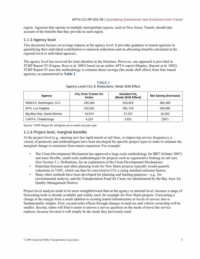
1.1.3 Agency level This document focuses on average impacts at the agency level. It provides guidance to transit agencies in quantifying their individual contribution to emission reductions and on allocating benefits calculated at the regional level to individual agencies.
The agency level has received the least attention in the literature. However, one approach is provided in TCRP Report 93 (Feigon, Hoyt et al. 2003) based on an earlier APTA report (Shapiro, Hassett et al. 2002). TCRP Report 93 uses this methodology to estimate direct savings (the mode shift effect) from four transit agencies, as summarized in Table 1.
TABLE 1 Agency-Level CO2-E Reductions, Mode Shift Effect
Agency CO2 from Transit Ve-hicles
Avoided CO2(Mode Shift Effect) Net Saving (Increase)
WMATA, Washington, D.C. 255,364 615,823 360,459
MTA, Los Angeles 242,061 581,743 339,682
Big Blue Bus, Santa Monica 10,974 27,237 16,263
CARTA, Chattanooga 4,219 3,631 (587)
Source: TCRP Report 93. All figures are in metric tons per year.
1.1.4 Project level, marginal benefits At the project level (e.g., opening new bus rapid transit or rail lines, or improving service frequency), a variety of protocols and methodologies have been developed for specific project types in order to estimate the marginal change in emissions from transit expansion. For example:
• The Clean Development Mechanism has approved a large-scale methodology for BRT (Grütter 2007) and more flexible, small-scale methodologies for projects such as regenerative braking on rail cars. (See Section 3.1, Definitions, for an explanation of the Clean Development Mechanism).
• Ridership forecasts and other planning work for New Starts projects typically would quantify reductions in VMT, which can then be converted to CO2-e using standard emission factors.
• Many other methods have been developed for planning and funding purposes—e.g., for environmental analysis, and the Transportation Fund for Clean Air administered by the Bay Area Air Quality Management District.
Project-level analysis tends to be more straightforward than at the agency or national level, because a range of forecasting tools is already available and widely used, for example for New Starts projects. Forecasting a change at the margin from a small addition to existing transit infrastructure or levels of service also is fundamentally simpler. First, second-order effects through changes in land use and vehicle ownership will be smaller. Second, riders will find it easier to answer a survey question on the mode of travel the service replaces, because for most it will simply be the mode they previously used.
APTA-CC-RP-001-09 | Quantifying Greenhouse Gas Emissions from Transit
© 2009 American Public Transportation Association 4
1.2 Why quantify emissions? There are several reasons why a transit agency might want to comprehensively quantify its greenhouse gas emissions:
1. Communicating the benefits of transit. Recent studies have demonstrated the role of transit in addressing climate change and its related benefits on a national level (http://www.apta.com/research/info/online/ greenhouse_brochure.cfm). By quantifying their net emissions in a standardized, rigorous manner, agencies can communicate their contributions to elected officials and to the wider community, especially as local, state and federal policy seeks to address transportation’s role in contributing to climate change.
2. Ensuring eligibility for new funding sources. Climate change policy may open up several new sources of funding for transit and vehicle trip reduction programs. Examples might include developer-funded transit improvements to mitigate GHG impacts of new projects under state environmental legislation; potential grant programs for emission reduction projects, such as FTA’s TIGGER program under ARRA; and the sale of emission reductions (offsets) on carbon markets. All of these require the quantification of emission savings, and completing this protocol will allow transit agencies to have readily accessible data for these funding sources.
3. Reporting to carbon accounting and trading organizations, such as The Climate Registry and the Chicago Climate Exchange. Organizations such as The Climate Registry maintain inventories of greenhouse gas emissions based on standardized protocols. In most cases, reporting is voluntary. However, some states have passed or are considering regulations that would mandate reporting to The Climate Registry for large emitters, and there may be benefits for organizations that can demonstrate that they have taken early action to reduce emissions. While the Chicago Climate Exchange is a trading organization, its members also need to report their emissions.
4. Setting emissions targets in local/regional climate action plans. Many localities and regions are creating climate action plans that identify strategies for reducing emissions. The Recommended Practice will assist agencies in evaluating and demonstrating the regional emission reductions they can contribute. This in turn can result in additional policy, programmatic and/or financial support for the provision of transit and supporting activities.
5. Supporting internal efforts to reduce emissions. Many transit agencies have goals to reduce greenhouse gas emissions, both from their own operations and from the wider community. This guidance can help ensure that emissions are reported in a standardized way, allowing agencies to track their efforts and benchmark themselves against other agencies. In particular, this methodology will be the basis for GHG measurement in the APTA Sustainability Commitment, currently in its pilot phase.
Depending on the purpose, different categories of emissions may be included. For example, inventories such as The Climate Registry consider only direct and indirect emissions from transit agencies, defined in the following section, and would not include displaced emissions from mode shift, congestion relief or land-use changes (although these could still be reported as optional information).
1.3 Emission scopes Emission inventory protocols such as those developed by The Climate Registry (2008) and World Resources Institute (2004) make a key distinction between three “scopes” of emissions:
• Scope 1: Direct emissions. This scope includes: • stationary combustion from boilers and furnaces;
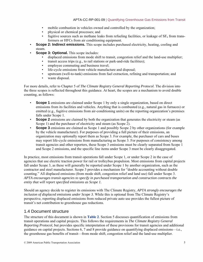
APTA-CC-RP-001-09 | Quantifying Greenhouse Gas Emissions from Transit
© 2009 American Public Transportation Association 5
• mobile combustion in vehicles owned and controlled by the organization; • physical or chemical processes; and • fugitive sources such as methane leaks from refueling facilities, or leakage of SF6 from trans-
formers or HFCs from air conditioning equipment. • Scope 2: Indirect emissions. This scope includes purchased electricity, heating, cooling and
steam. • Scope 3: Optional. This scope includes:
• displaced emissions from mode shift to transit, congestion relief and the land-use multiplier; • transit access trips (e.g., to rail stations or park-and-ride facilities); • employee commuting and business travel; • life-cycle emissions from vehicle manufacture and disposal; • upstream (well-to-tank) emissions from fuel extraction, refining and transportation; and • waste disposal.
For more details, refer to Chapter 5 of The Climate Registry General Reporting Protocol. The division into the three scopes is reflected throughout this guidance. At heart, the scopes are a mechanism to avoid double counting, as follows:
• Scope 1 emissions are claimed under Scope 1 by only a single organization, based on direct emissions from its facilities and vehicles. Anything that is combusted (e.g., natural gas in furnaces) or emitted (e.g., fugitive emissions from air-conditioning units) on the reporting organization’s premises falls under Scope 1.
• Scope 2 emissions are claimed by both the organization that generates the electricity or steam (as Scope 1) and the purchaser of electricity and steam (as Scope 2).
• Scope 3 emissions are claimed as Scope 1 and possibly Scope 2 by other organizations (for example by the vehicle manufacturer). For purposes of providing a full picture of their emissions, an organization may optionally report them as Scope 3. For example, the purchaser of cars and buses may report life-cycle emissions from manufacturing as Scope 3. For purposes of consistency among transit agencies and other reporters, these Scope 3 emissions must be clearly separated from Scope 1 and Scope 2 emissions, and the specific line items under Scope 3 must be clearly disaggregated.
In practice, most emissions from transit operations fall under Scope 1, or under Scope 2 in the case of agencies that use electric traction power for rail or trolleybus propulsion. Most emissions from capital projects fall under Scope 3, as these will generally be reported under Scope 1 by another organization, such as the contractor and steel manufacturer. Scope 3 provides a mechanism for “double accounting without double counting.” All displaced emissions (from mode shift, congestion relief and land use) fall under Scope 3. APTA encourages transit agencies to specify in purchased transportation and construction contracts the entity that will report specified emissions as Scope 1.
Should an agency decide to register its emissions with The Climate Registry, APTA strongly encourages the inclusion of displaced emissions under Scope 3. While this is optional from The Climate Registry’s perspective, reporting displaced emissions from reduced private auto use provides the fullest picture of transit’s net contribution to greenhouse gas reductions.
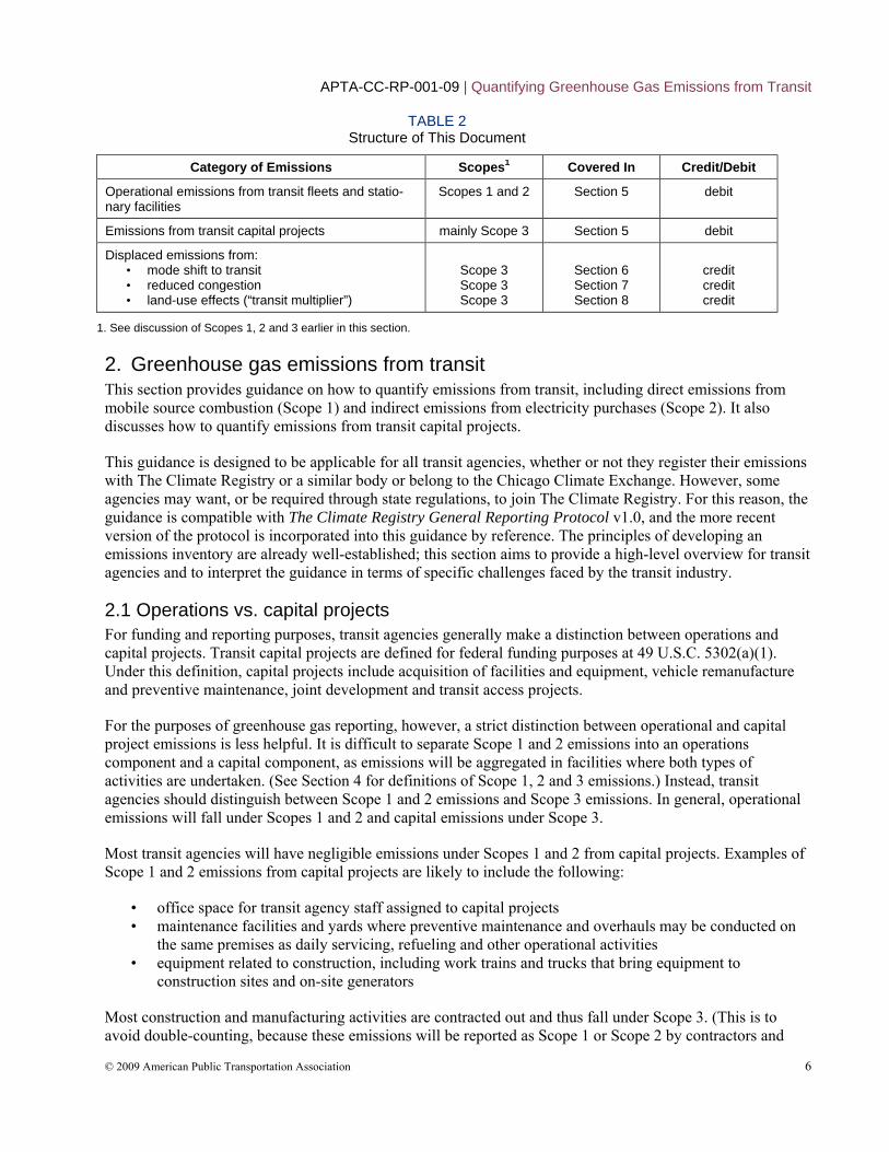
1.4 Document structure The structure of this document is shown in Table 2. Section 5 discusses quantification of emissions from transit operations and capital projects. This follows the requirements in The Climate Registry General Reporting Protocol, but provides specific interpretation of these provisions for transit agencies and additional guidance on capital projects. Sections 6, 7 and 8 provide guidance on quantifying displaced emissions—i.e., the greenhouse gas benefits of transit—from mode shift, congestion relief and the land-use multiplier.
APTA-CC-RP-001-09 | Quantifying Greenhouse Gas Emissions from Transit
© 2009 American Public Transportation Association 6
TABLE 2 Structure of This Document
Category of Emissions Scopes1 Covered In Credit/Debit
Operational emissions from transit fleets and statio-nary facilities
Scopes 1 and 2 Section 5 debit
Emissions from transit capital projects mainly Scope 3 Section 5 debit
Displaced emissions from: • mode shift to transit • reduced congestion • land-use effects (“transit multiplier”)
Scope 3 Scope 3 Scope 3
Section 6 Section 7 Section 8
credit credit credit
1. See discussion of Scopes 1, 2 and 3 earlier in this section.
2. Greenhouse gas emissions from transit This section provides guidance on how to quantify emissions from transit, including direct emissions from mobile source combustion (Scope 1) and indirect emissions from electricity purchases (Scope 2). It also discusses how to quantify emissions from transit capital projects.
This guidance is designed to be applicable for all transit agencies, whether or not they register their emissions with The Climate Registry or a similar body or belong to the Chicago Climate Exchange. However, some agencies may want, or be required through state regulations, to join The Climate Registry. For this reason, the guidance is compatible with The Climate Registry General Reporting Protocol v1.0, and the more recent version of the protocol is incorporated into this guidance by reference. The principles of developing an emissions inventory are already well-established; this section aims to provide a high-level overview for transit agencies and to interpret the guidance in terms of specific challenges faced by the transit industry.
2.1 Operations vs. capital projects For funding and reporting purposes, transit agencies generally make a distinction between operations and capital projects. Transit capital projects are defined for federal funding purposes at 49 U.S.C. 5302(a)(1). Under this definition, capital projects include acquisition of facilities and equipment, vehicle remanufacture and preventive maintenance, joint development and transit access projects.
For the purposes of greenhouse gas reporting, however, a strict distinction between operational and capital project emissions is less helpful. It is difficult to separate Scope 1 and 2 emissions into an operations component and a capital component, as emissions will be aggregated in facilities where both types of activities are undertaken. (See Section 4 for definitions of Scope 1, 2 and 3 emissions.) Instead, transit agencies should distinguish between Scope 1 and 2 emissions and Scope 3 emissions. In general, operational emissions will fall under Scopes 1 and 2 and capital emissions under Scope 3.
Most transit agencies will have negligible emissions under Scopes 1 and 2 from capital projects. Examples of Scope 1 and 2 emissions from capital projects are likely to include the following:
• office space for transit agency staff assigned to capital projects • maintenance facilities and yards where preventive maintenance and overhauls may be conducted on
the same premises as daily servicing, refueling and other operational activities • equipment related to construction, including work trains and trucks that bring equipment to
construction sites and on-site generators
Most construction and manufacturing activities are contracted out and thus fall under Scope 3. (This is to avoid double-counting, because these emissions will be reported as Scope 1 or Scope 2 by contractors and
APTA-CC-RP-001-09 | Quantifying Greenhouse Gas Emissions from Transit
© 2009 American Public Transportation Association 7
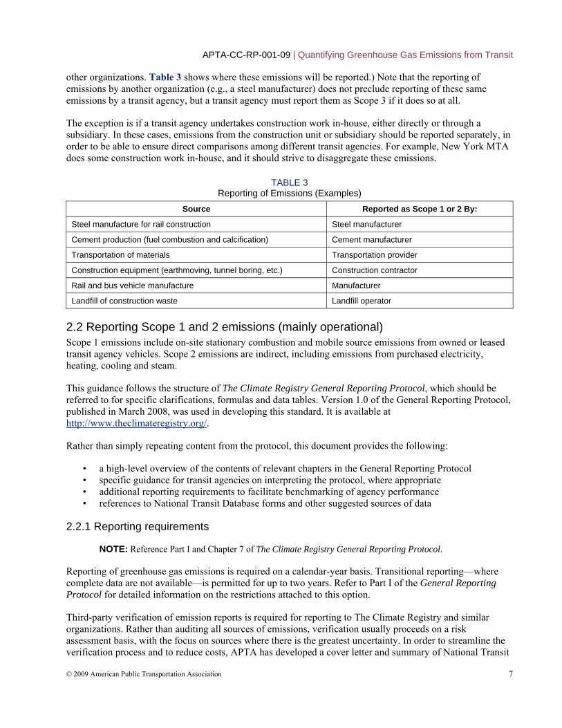
other organizations. Table 3 shows where these emissions will be reported.) Note that the reporting of emissions by another organization (e.g., a steel manufacturer) does not preclude reporting of these same emissions by a transit agency, but a transit agency must report them as Scope 3 if it does so at all.
The exception is if a transit agency undertakes construction work in-house, either directly or through a subsidiary. In these cases, emissions from the construction unit or subsidiary should be reported separately, in order to be able to ensure direct comparisons among different transit agencies. For example, New York MTA does some construction work in-house, and it should strive to disaggregate these emissions.
TABLE 3 Reporting of Emissions (Examples)
Source Reported as Scope 1 or 2 By:
Steel manufacture for rail construction Steel manufacturer
Cement production (fuel combustion and calcification) Cement manufacturer
Transportation of materials Transportation provider
Construction equipment (earthmoving, tunnel boring, etc.) Construction contractor
Rail and bus vehicle manufacture Manufacturer
Landfill of construction waste Landfill operator
2.2 Reporting Scope 1 and 2 emissions (mainly operational) Scope 1 emissions include on-site stationary combustion and mobile source emissions from owned or leased transit agency vehicles. Scope 2 emissions are indirect, including emissions from purchased electricity, heating, cooling and steam.
This guidance follows the structure of The Climate Registry General Reporting Protocol, which should be referred to for specific clarifications, formulas and data tables. Version 1.0 of the General Reporting Protocol, published in March 2008, was used in developing this standard. It is available at http://www.theclimateregistry.org/.
Rather than simply repeating content from the protocol, this document provides the following:
• a high-level overview of the contents of relevant chapters in the General Reporting Protocol • specific guidance for transit agencies on interpreting the protocol, where appropriate • additional reporting requirements to facilitate benchmarking of agency performance • references to National Transit Database forms and other suggested sources of data
2.2.1 Reporting requirements
NOTE: Reference Part I and Chapter 7 of The Climate Registry General Reporting Protocol.
Reporting of greenhouse gas emissions is required on a calendar-year basis. Transitional reporting—where complete data are not available—is permitted for up to two years. Refer to Part I of the General Reporting Protocol for detailed information on the restrictions attached to this option.
Third-party verification of emission reports is required for reporting to The Climate Registry and similar organizations. Rather than auditing all sources of emissions, verification usually proceeds on a risk assessment basis, with the focus on sources where there is the greatest uncertainty. In order to streamline the verification process and to reduce costs, APTA has developed a cover letter and summary of National Transit
APTA-CC-RP-001-09 | Quantifying Greenhouse Gas Emissions from Transit
© 2009 American Public Transportation Association 8
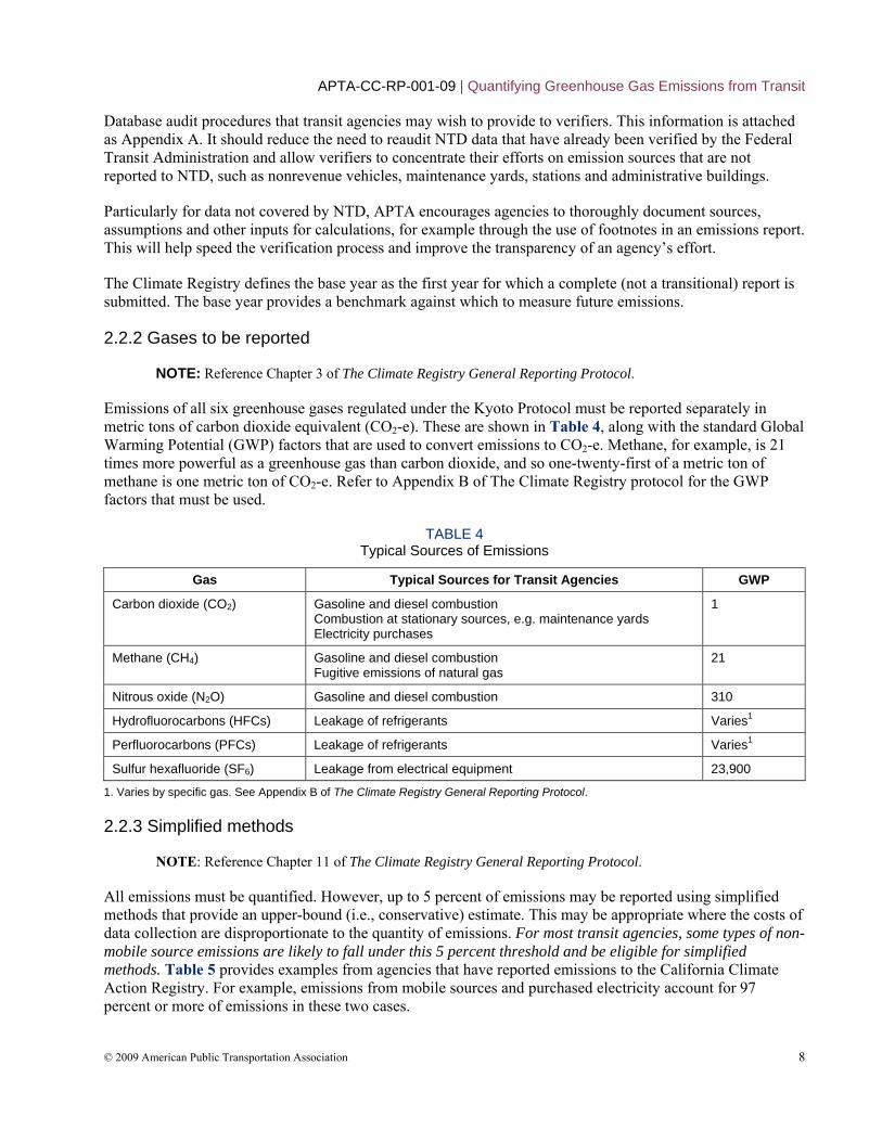
Database audit procedures that transit agencies may wish to provide to verifiers. This information is attached as Appendix A. It should reduce the need to reaudit NTD data that have already been verified by the Federal Transit Administration and allow verifiers to concentrate their efforts on emission sources that are not reported to NTD, such as nonrevenue vehicles, maintenance yards, stations and administrative buildings.
Particularly for data not covered by NTD, APTA encourages agencies to thoroughly document sources, assumptions and other inputs for calculations, for example through the use of footnotes in an emissions report. This will help speed the verification process and improve the transparency of an agency’s effort.
The Climate Registry defines the base year as the first year for which a complete (not a transitional) report is submitted. The base year provides a benchmark against which to measure future emissions.
2.2.2 Gases to be reported
NOTE: Reference Chapter 3 of The Climate Registry General Reporting Protocol.
Emissions of all six greenhouse gases regulated under the Kyoto Protocol must be reported separately in metric tons of carbon dioxide equivalent (CO2-e). These are shown in Table 4, along with the standard Global Warming Potential (GWP) factors that are used to convert emissions to CO2-e. Methane, for example, is 21 times more powerful as a greenhouse gas than carbon dioxide, and so one-twenty-first of a metric ton of methane is one metric ton of CO2-e. Refer to Appendix B of The Climate Registry protocol for the GWP factors that must be used.
TABLE 4 Typical Sources of Emissions
Gas Typical Sources for Transit Agencies GWP
Carbon dioxide (CO2) Gasoline and diesel combustion Combustion at stationary sources, e.g. maintenance yards Electricity purchases
1
Methane (CH4) Gasoline and diesel combustion Fugitive emissions of natural gas
21
Nitrous oxide (N2O) Gasoline and diesel combustion 310
Hydrofluorocarbons (HFCs) Leakage of refrigerants Varies1
Perfluorocarbons (PFCs) Leakage of refrigerants Varies1
Sulfur hexafluoride (SF6) Leakage from electrical equipment 23,900
1. Varies by specific gas. See Appendix B of The Climate Registry General Reporting Protocol.
2.2.3 Simplified methods
NOTE: Reference Chapter 11 of The Climate Registry General Reporting Protocol.
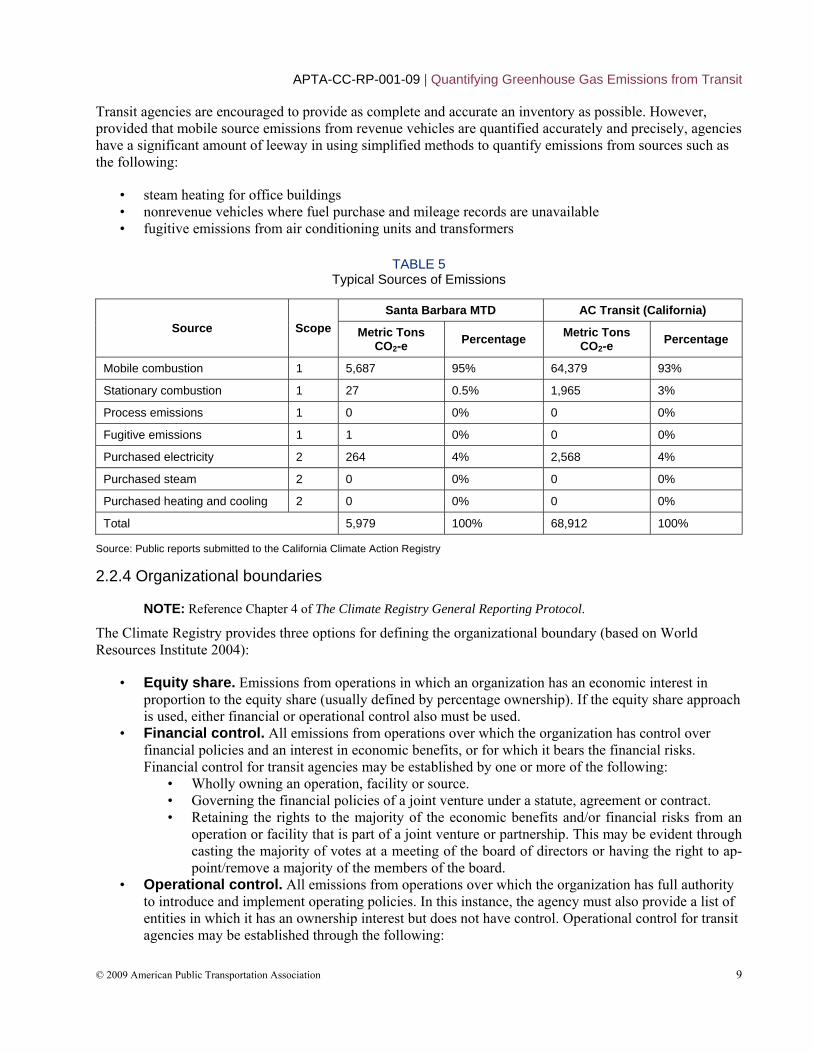
All emissions must be quantified. However, up to 5 percent of emissions may be reported using simplified methods that provide an upper-bound (i.e., conservative) estimate. This may be appropriate where the costs of data collection are disproportionate to the quantity of emissions. For most transit agencies, some types of non-mobile source emissions are likely to fall under this 5 percent threshold and be eligible for simplified methods. Table 5 provides examples from agencies that have reported emissions to the California Climate Action Registry. For example, emissions from mobile sources and purchased electricity account for 97 percent or more of emissions in these two cases.
APTA-CC-RP-001-09 | Quantifying Greenhouse Gas Emissions from Transit
© 2009 American Public Transportation Association 9
Transit agencies are encouraged to provide as complete and accurate an inventory as possible. However, provided that mobile source emissions from revenue vehicles are quantified accurately and precisely, agencies have a significant amount of leeway in using simplified methods to quantify emissions from sources such as the following:
• steam heating for office buildings • nonrevenue vehicles where fuel purchase and mileage records are unavailable • fugitive emissions from air conditioning units and transformers
TABLE 5 Typical Sources of Emissions
Source Scope Santa Barbara MTD AC Transit (California)
Metric Tons CO2-e Percentage Metric Tons
CO2-e Percentage
Mobile combustion 1 5,687 95% 64,379 93%
Stationary combustion 1 27 0.5% 1,965 3%
Process emissions 1 0 0% 0 0%
Fugitive emissions 1 1 0% 0 0%
Purchased electricity 2 264 4% 2,568 4%
Purchased steam 2 0 0% 0 0%
Purchased heating and cooling 2 0 0% 0 0%
Total 5,979 100% 68,912 100%
Source: Public reports submitted to the California Climate Action Registry
2.2.4 Organizational boundaries
NOTE: Reference Chapter 4 of The Climate Registry General Reporting Protocol.
The Climate Registry provides three options for defining the organizational boundary (based on World Resources Institute 2004):
• Equity share. Emissions from operations in which an organization has an economic interest in proportion to the equity share (usually defined by percentage ownership). If the equity share approach is used, either financial or operational control also must be used.
• Financial control. All emissions from operations over which the organization has control over financial policies and an interest in economic benefits, or for which it bears the financial risks. Financial control for transit agencies may be established by one or more of the following:
• Wholly owning an operation, facility or source. • Governing the financial policies of a joint venture under a statute, agreement or contract. • Retaining the rights to the majority of the economic benefits and/or financial risks from an
operation or facility that is part of a joint venture or partnership. This may be evident through casting the majority of votes at a meeting of the board of directors or having the right to ap-point/remove a majority of the members of the board.
• Operational control. All emissions from operations over which the organization has full authority to introduce and implement operating policies. In this instance, the agency must also provide a list of entities in which it has an ownership interest but does not have control. Operational control for transit agencies may be established through the following:
APTA-CC-RP-001-09 | Quantifying Greenhouse Gas Emissions from Transit
© 2009 American Public Transportation Association 10
• Wholly owning an operation, facility or source. • Having the full authority to introduce and implement operational and health, safety and envi-
ronmental policies.
APTA strongly recommends that transit agencies use the operational control method to report their emissions. This provides the most appropriate match with their emissions and is also the regulatory approach being considered in some states, including California.
In many cases, organizational boundaries involve a gray area, and definitions of operational and financial control are subject to interpretation. In almost all cases, however, the following rule should apply: If a transit agency reports data on a service to the National Transit Database, it should be considered to have operational control over these emissions. For example:
• Directly operated services clearly fall under an agency’s operational control. • Purchased transportation services fall under an agency’s operational control, as the agency
specifies routes, service frequencies, vehicle and fuel types, and health and safety policies. This applies to services purchased from another transit agency or from a private contractor.
• Paratransit services provided under the Americans with Disabilities Act (ADA) fall under an agency’s operational control, as the agency specifies service policies, eligibility (subject to federal law), vehicle standards, fuel types and health and safety policies.
• Vanpool services reported to NTD—where the transit agency specifies destinations, vehicle standards, fuel types and health and safety policies, and may also own or lease the vehicle—also fall under an agency’s operation control.
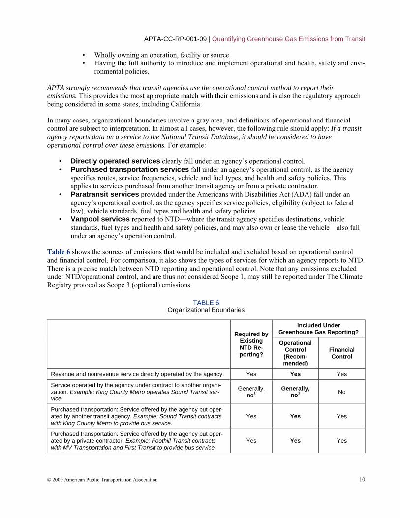
Table 6 shows the sources of emissions that would be included and excluded based on operational control and financial control. For comparison, it also shows the types of services for which an agency reports to NTD. There is a precise match between NTD reporting and operational control. Note that any emissions excluded under NTD/operational control, and are thus not considered Scope 1, may still be reported under The Climate Registry protocol as Scope 3 (optional) emissions.
TABLE 6 Organizational Boundaries
Required by
Existing NTD Re-porting?
Included UnderGreenhouse Gas Reporting?
Operational Control (Recom-mended)
Financial Control
Revenue and nonrevenue service directly operated by the agency. Yes Yes Yes
Service operated by the agency under contract to another organi-zation. Example: King County Metro operates Sound Transit ser-vice.
Generally, no1
Generally, no1 No
Purchased transportation: Service offered by the agency but oper-ated by another transit agency. Example: Sound Transit contracts with King County Metro to provide bus service.
Yes Yes Yes
Purchased transportation: Service offered by the agency but oper-ated by a private contractor. Example: Foothill Transit contracts with MV Transportation and First Transit to provide bus service.
Yes Yes Yes
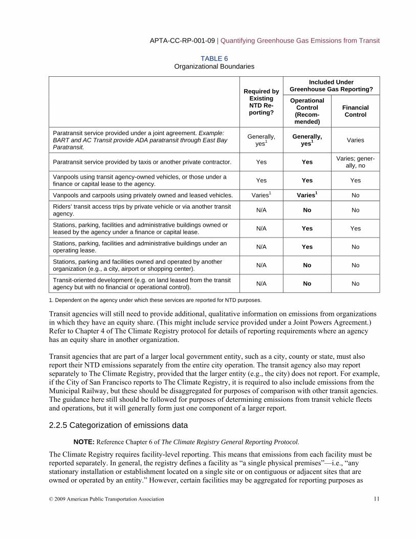
APTA-CC-RP-001-09 | Quantifying Greenhouse Gas Emissions from Transit
© 2009 American Public Transportation Association 11
TABLE 6 Organizational Boundaries
Required by
Existing NTD Re-porting?
Included UnderGreenhouse Gas Reporting?
Operational Control (Recom-mended)
Financial Control
Paratransit service provided under a joint agreement. Example: BART and AC Transit provide ADA paratransit through East Bay Paratransit.
Generally, yes1
Generally, yes1 Varies
Paratransit service provided by taxis or another private contractor. Yes Yes Varies; gener-ally, no
Vanpools using transit agency-owned vehicles, or those under a finance or capital lease to the agency. Yes Yes Yes
Vanpools and carpools using privately owned and leased vehicles. Varies1 Varies1 No
Riders’ transit access trips by private vehicle or via another transit agency. N/A No No
Stations, parking, facilities and administrative buildings owned or leased by the agency under a finance or capital lease. N/A Yes Yes
Stations, parking, facilities and administrative buildings under an operating lease. N/A Yes No
Stations, parking and facilities owned and operated by another organization (e.g., a city, airport or shopping center). N/A No No
Transit-oriented development (e.g. on land leased from the transit agency but with no financial or operational control). N/A No No
1. Dependent on the agency under which these services are reported for NTD purposes.
Transit agencies will still need to provide additional, qualitative information on emissions from organizations in which they have an equity share. (This might include service provided under a Joint Powers Agreement.) Refer to Chapter 4 of The Climate Registry protocol for details of reporting requirements where an agency has an equity share in another organization.
Transit agencies that are part of a larger local government entity, such as a city, county or state, must also report their NTD emissions separately from the entire city operation. The transit agency also may report separately to The Climate Registry, provided that the larger entity (e.g., the city) does not report. For example, if the City of San Francisco reports to The Climate Registry, it is required to also include emissions from the Municipal Railway, but these should be disaggregated for purposes of comparison with other transit agencies. The guidance here still should be followed for purposes of determining emissions from transit vehicle fleets and operations, but it will generally form just one component of a larger report.
2.2.5 Categorization of emissions data
NOTE: Reference Chapter 6 of The Climate Registry General Reporting Protocol.
The Climate Registry requires facility-level reporting. This means that emissions from each facility must be reported separately. In general, the registry defines a facility as “a single physical premises”—i.e., “any stationary installation or establishment located on a single site or on contiguous or adjacent sites that are owned or operated by an entity.” However, certain facilities may be aggregated for reporting purposes as
APTA-CC-RP-001-09 | Quantifying Greenhouse Gas Emissions from Transit
© 2009 American Public Transportation Association 12
follows (note that nothing precludes reporting on a more disaggregated basis should a transit agency have available data):
• Commercial buildings. Offices, sales outlets, customer service facilities, maintenance yards and administrative facilities may be aggregated and reported as a single facility. This will capture most of an agency’s emissions from stationary sources, with the exception of stations. Ideally, maintenance yards should be disaggregated, but this is not required.
NOTE: The Climate Registry protocol allows aggregation for commercial buildings, but not for indus-trial buildings. However, the precise definition of commercial buildings is unclear. Examples of com-mercial buildings include “office buildings, retail stores, storage facilities, etc.,” while examples of in-dustrial buildings include factories, mills and power plants.
• Stations. Stations and other emissions on a contiguous right-of-way (e.g., signals that draw power from the electrified rail, if these are not counted under traction power) may be reported as a single facility, analogous to a pipeline. If data are available on individual stations, agencies are encouraged to disaggregate emissions further.
NOTE: According to The Climate Registry protocol (p. 39): “The Registry understands that some emission sources, such as pipelines and electricity transmission and distribution (T&D) systems, do not easily conform to this traditional definition of a facility…. For purposes of reporting, each pipeline, pipeline system, or electricity T&D system should be treated as a single facility.” APTA has requested that The Climate Registry confirm that transit rights of way qualify as a single facility under this provi-sion.
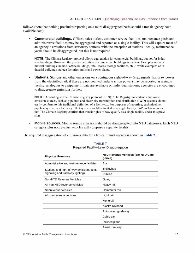
• Mobile sources. Mobile source emissions should be disaggregated into NTD categories. Each NTD category plus nonrevenue vehicles will comprise a separate facility.
The required disaggregation of emissions data for a typical transit agency is shown in Table 7.
TABLE 7 Required Facility-Level Disaggregation
Physical Premises NTD Revenue Vehicles (per NTD Cate-gories)
Administrative and maintenance facilities Bus
Stations and right-of-way emissions (e.g. signaling and trackway lighting)
Trolleybus
Publico
Non-NTD Revenue Vehicles Jitney
All non-NTD revenue vehicles Heavy rail
Nonrevenue Vehicles Commuter rail
All non-revenue vehicles Light rail
Monorail
Alaska Railroad
Automated guideway
Cable car
Inclined plane
Aerial tramway
APTA-CC-RP-001-09 | Quantifying Greenhouse Gas Emissions from Transit
© 2009 American Public Transportation Association 13
Demand response (e.g., paratransit)
Vanpool
Ferry
Other NTD revenue vehicle
Note that emissions also must be disaggregated by state for purposes of reporting to The Climate Registry. This applies only to transit agencies that report stationary emissions sources (such as a maintenance yard) in more than one state. Agencies that operate across state lines and have mobile source emissions or right-of-way in more than one state (e.g., New Jersey Transit running service into New York) may choose to disaggregate these types of emissions by state, or simply report them as a single “United States” category.
2.2.6 Performance metrics
NOTE: Reference Chapter 17 of The Climate Registry General Reporting Protocol.
Performance metrics are optional under The Climate Registry protocol. However, in order to facilitate benchmarking of transit agencies, this standard requires the following metrics to be reported for both each National Transit Database modal category, and for the agency as a whole:
• Emissions per vehicle mile (revenue service plus deadhead segments). This primarily measures vehicle efficiency and will be sensitive to efforts to purchase lower-emission vehicles or to switch to lower-carbon fuels.
• Emissions per revenue vehicle hour. This is another measure of operational efficiency, but will take into account efforts to reduce deadheading. It also takes into account congestion, which will depress performance on emissions per vehicle mile.
• Emissions per passenger mile. This takes into account service productivity and will reward increases in ridership and load factors.
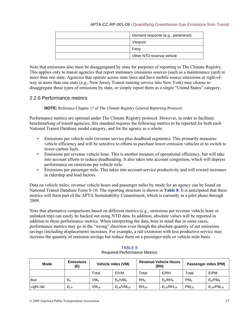
Data on vehicle miles, revenue vehicle hours and passenger miles by mode for an agency can be found on National Transit Database Form S-10. The reporting structure is shown in Table 8. It is anticipated that these metrics will form part of the APTA Sustainability Commitment, which is currently in a pilot phase through 2009.
Note that alternative comparisons based on different metrics (e.g., emissions per revenue vehicle hour or unlinked trip) can easily be backed out using NTD data. In addition, absolute values will be reported in addition to these performance metrics. When interpreting the data, bear in mind that in some cases, performance metrics may go in the “wrong” direction even though the absolute quantity of net emissions savings (including displacement) increases. For example, a rail extension with less productive service may increase the quantity of emission savings but reduce them on a passenger-mile or vehicle-mile basis.
TABLE 8 Required Performance Metrics
Mode Emissions (E) Vehicle miles (VM) Revenue Vehicle Hours
(RH) Passenger miles (PM)
Total E/VM Total E/RH Total E/PM
Bus Eb VMb Eb/VMb RHb Eb/RHb PMb Eb/PMb
Light rail ELR VMLR ELR/VMLR RHLR ELR/RHLR PMLR ELR/PMLR
APTA-CC-RP-001-09 | Quantifying Greenhouse Gas Emissions from Transit
© 2009 American Public Transportation Association 14
[repeat for other NTD modes]
Nonrevenue ENR
Stationary sources Estationary
Total1 Etot VMtot Etot/VMtot RHtot Etot/RHtot PMtot Etot/Ptot
1. Including emissions from stationary sources.
2.2.7 Quantifying emissions This section provides guidance on quantifying emissions from five types of sources:
• direct emissions from stationary combustion (e.g., on-site furnaces) • direct emissions from mobile combustion • indirect emissions from electricity use • other indirect emissions (e.g., steam purchases) • fugitive emissions (e.g., refrigerant leaks)
In most cases, data will be available for all transit agencies through NTD reporting, fuel purchases and similar records. However, should this not be the case, simplified methods may be used, provided that the emissions total 5 percent or less of the agency’s total emissions. For more details, see Chapter 11 of The Climate Registry protocol.
Emissions from biofuels such as ethanol and biodiesel must be reported in full as part of Scope 1. However, The Climate Registry also requires CO2 emissions from biofuels to be reported separately. In other words, Scope 1 emissions will be divided into fossil-based (regular gasoline and diesel) and biogenic (biofuels).
2.2.8 Direct emissions from stationary combustion
NOTE: Reference Chapter 12 of The Climate Registry General Reporting Protocol.
The following are typical stationary combustion sources for transit agencies:
• boilers • furnaces • on-site generation
The Climate Registry provides several options (“tiers”) for quantifying direct emissions from stationary combustion. Given the small share of emissions from stationary sources, most transit agencies will find it appropriate to use Tier C, using default emission factors for each fuel type.
NOTE: In general, Tier A provides the most precise estimates but is most demanding in terms of data. Tier C is less data-intensive and often relies on default factors.
In general, data on direct emissions from stationary combustion will not be available through NTD reporting. Agencies should determine annual fuel use by reading individual meters or by using fuel receipts or purchase records together with data on changes in stocks. Emissions must be calculated separately for each facility as described above. Refer to Chapter 12 of The Climate Registry protocol for detailed directions and default emission factors.
Emissions for each fuel type (A, B, etc.) are calculated using the following formulas:
APTA-CC-RP-001-09 | Quantifying Greenhouse Gas Emissions from Transit
© 2009 American Public Transportation Association 15
Total annual Fuel A consumption = Annual fuel purchases – Annual fuel sales + Fuel stock at beginning of year – Fuel stock at end of year
Fuel A CO2 Emissions = Fuel consumed × CO2 emission factor / 1000
Fuel A N2O Emissions = Fuel consumed × N2O emission factor / 1,000,000
Fuel A CH4 Emissions = Fuel consumed × CH4 emission factor / 1,000,000
NOTE: Throughout this part of the report, the denominators (1000, 1,000,000, etc.) simply normalize CO2 emissions into standard units (metric tons of CO2), depending on the units of the original data and emission factors.
2.2.9 Direct emissions from mobile combustion
NOTE: Reference Chapter 13 of The Climate Registry General Reporting Protocol.
Typical sources of mobile combustion emissions for transit agencies include the following:
• revenue vehicles • nonrevenue vehicles
This category includes vehicles fueled by natural gas and biofuels, but not electric traction where the electricity is generated off-site (and is thus classified as Scope 2).
Note that biogenic (e.g., biodiesel) emissions must be reported separately. For blended fuels (e.g., B20), fossil and biogenic emissions must be disaggregated. Under The Climate Registry protocol, emissions are measured on an organizational basis, and transit agencies must report actual emissions at the point of combustion. No account is taken of reduced life-cycle emissions from biogenic sources, such as carbon sequestered during the growing of the crop.
Also note that well-to-tank emissions from fuel extraction, refining and transportation are not considered. If an agency wishes to estimate these emissions, for example using GREET or a similar model, they would be considered Scope 3 and must be reported separately.
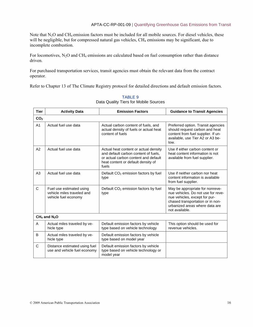
The Climate Registry provides several tiers for quantifying direct emissions from mobile combustion. In general, agencies should use Tier A, subject to the guidance in Table 9. Table 10 shows data sources and National Transit Database references.
When actual fuel use, fuel carbon content and heat content data are available, emissions for each fuel type (A, B, etc.) are calculated using the following formulas:
Total annual Fuel A consumption = Annual fuel purchases + Fuel stock at beginning of year – Fuel stock at end of year
Fuel A CO2 emissions = Heat content × Carbon content × % oxidized × 44 / 12 / 1000
Fuel A N2O emissions = Annual distance driven × N2O emission factor / 1,000,000
Fuel A CH4 emissions = Annual distance driven × CH4 emission factor / 1,000,000
NOTE: 44 / 12 converts from carbon into CO2, based on their relative molecular weights (C = 12, O = 16).
APTA-CC-RP-001-09 | Quantifying Greenhouse Gas Emissions from Transit
© 2009 American Public Transportation Association 16
Note that N2O and CH4 emission factors must be included for all mobile sources. For diesel vehicles, these will be negligible, but for compressed natural gas vehicles, CH4 emissions may be significant, due to incomplete combustion.
For locomotives, N2O and CH4 emissions are calculated based on fuel consumption rather than distance driven.
For purchased transportation services, transit agencies must obtain the relevant data from the contract operator.
Refer to Chapter 13 of The Climate Registry protocol for detailed directions and default emission factors.
TABLE 9 Data Quality Tiers for Mobile Sources
Tier Activity Data Emission Factors Guidance to Transit Agencies
CO2
A1 Actual fuel use data Actual carbon content of fuels, and actual density of fuels or actual heat content of fuels
Preferred option. Transit agencies should request carbon and heat content from fuel supplier. If un-available, use Tier A2 or A3 be-low.
A2 Actual fuel use data Actual heat content or actual density and default carbon content of fuels, or actual carbon content and default heat content or default density of fuels
Use if either carbon content or heat content information is not available from fuel supplier.
A3 Actual fuel use data Default CO2 emission factors by fuel type
Use if neither carbon nor heat content information is available from fuel supplier.
C Fuel use estimated using vehicle miles traveled and vehicle fuel economy
Default CO2 emission factors by fuel type
May be appropriate for nonreve-nue vehicles. Do not use for reve-nue vehicles, except for pur-chased transportation or in non-urbanized areas where data are not available.
CH4 and N2O
A Actual miles traveled by ve-hicle type
Default emission factors by vehicle type based on vehicle technology
This option should be used for revenue vehicles.
B Actual miles traveled by ve-hicle type
Default emission factors by vehicle type based on model year
C Distance estimated using fuel use and vehicle fuel economy
Default emission factors by vehicle type based on vehicle technology or model year
APTA-CC-RP-001-09 | Quantifying Greenhouse Gas Emissions from Transit
© 2009 American Public Transportation Association 17
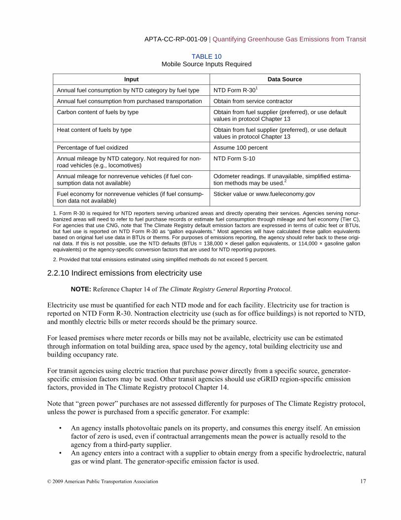
TABLE 10 Mobile Source Inputs Required
Input Data Source
Annual fuel consumption by NTD category by fuel type NTD Form R-301
Annual fuel consumption from purchased transportation Obtain from service contractor
Carbon content of fuels by type Obtain from fuel supplier (preferred), or use default values in protocol Chapter 13
Heat content of fuels by type Obtain from fuel supplier (preferred), or use default values in protocol Chapter 13
Percentage of fuel oxidized Assume 100 percent
Annual mileage by NTD category. Not required for non-road vehicles (e.g., locomotives)
NTD Form S-10
Annual mileage for nonrevenue vehicles (if fuel con-sumption data not available)
Odometer readings. If unavailable, simplified estima-tion methods may be used.2
Fuel economy for nonrevenue vehicles (if fuel consump-tion data not available)
Sticker value or www.fueleconomy.gov
1. Form R-30 is required for NTD reporters serving urbanized areas and directly operating their services. Agencies serving nonur-banized areas will need to refer to fuel purchase records or estimate fuel consumption through mileage and fuel economy (Tier C), For agencies that use CNG, note that The Climate Registry default emission factors are expressed in terms of cubic feet or BTUs,but fuel use is reported on NTD Form R-30 as “gallon equivalents.” Most agencies will have calculated these gallon equivalentsbased on original fuel use data in BTUs or therms. For purposes of emissions reporting, the agency should refer back to these origi-nal data. If this is not possible, use the NTD defaults (BTUs = 138,000 × diesel gallon equivalents, or 114,000 × gasoline gallon equivalents) or the agency-specific conversion factors that are used for NTD reporting purposes.
2. Provided that total emissions estimated using simplified methods do not exceed 5 percent.
2.2.10 Indirect emissions from electricity use
NOTE: Reference Chapter 14 of The Climate Registry General Reporting Protocol.
Electricity use must be quantified for each NTD mode and for each facility. Electricity use for traction is reported on NTD Form R-30. Nontraction electricity use (such as for office buildings) is not reported to NTD, and monthly electric bills or meter records should be the primary source.
For leased premises where meter records or bills may not be available, electricity use can be estimated through information on total building area, space used by the agency, total building electricity use and building occupancy rate.
For transit agencies using electric traction that purchase power directly from a specific source, generator-specific emission factors may be used. Other transit agencies should use eGRID region-specific emission factors, provided in The Climate Registry protocol Chapter 14.
Note that “green power” purchases are not assessed differently for purposes of The Climate Registry protocol, unless the power is purchased from a specific generator. For example:
• An agency installs photovoltaic panels on its property, and consumes this energy itself. An emission factor of zero is used, even if contractual arrangements mean the power is actually resold to the agency from a third-party supplier.
• An agency enters into a contract with a supplier to obtain energy from a specific hydroelectric, natural gas or wind plant. The generator-specific emission factor is used.
APTA-CC-RP-001-09 | Quantifying Greenhouse Gas Emissions from Transit
© 2009 American Public Transportation Association 18
• An agency purchases renewable energy through a utility’s “green power” program, or purchases renewable energy credits. No credit is given for the purchases, as this renewable energy is already reflected in the regional emission factor.
2.2.11 Other indirect emissions
NOTE: Reference Chapter 15 of The Climate Registry General Reporting Protocol.
These types of emissions include electricity, steam, heating or cooling purchases from a cogeneration plant, or a conventional boiler not owned by the agency. Refer to Chapter 15 of The Climate Registry protocol.
2.2.12 Fugitive emissions
NOTE: Reference Chapter 16 of The Climate Registry General Reporting Protocol.
Typical sources of fugitive emissions for transit agencies include the following:
• leakage from natural gas fueling facilities (although agencies may have automatic shutoff mechanisms that reduce this leakage to zero)
• leakage from air conditioning systems in buildings and stations (note that not all refrigerants are greenhouse gases—refer to Appendix B of The Climate Registry protocol)
• leakage from vehicle air conditioning systems (note that not all refrigerants are greenhouse gases—refer to Appendix B of The Climate Registry protocol)
• leakage from fire extinguishers • leakage from electrical systems such as transformers (SF6)
The Climate Registry protocol provides guidance on estimating fugitive emissions of HFCs and PFCs from air conditioning and refrigeration systems—e.g., air conditioning units on transit vehicles. Agencies that service their own units should have data on the quantity of refrigerants purchased and/or used. Other can use simplified estimation methods, provided that total emissions estimated using simplified methods do not exceed 5 percent of an organization’s inventory. Data still will be required on the capacity of each unit and the types of refrigerants that are used.
2.3 Reporting Scope 3 emissions (mainly capital) As discussed in Section 5.1, most emissions from transit capital projects will fall under Scope 3. These emissions are optional to report under The Climate Registry protocol, as they will generally fall under Scope 1 of another organization (e.g., the contractor). However, for benchmarking purposes and in the interests of providing information that is as complete as possible, it can be useful to estimate these emissions.
This guidance aims to provide a simple method to calculate emissions from capital projects that will be suitable for agencies of all types, regardless of size or types of capital investment pursued. It is not intended as a guide to conduct full life-cycle analysis of transit capital projects. For an example of this type of analysis, see Chester and Horvath (2007).
Note that Scope 3 emissions from transit should not be included when making modal comparisons, such as comparing transit emissions to private auto emissions per passenger mile. This is because auto emissions calculations generally do not include emissions such as highway construction and vehicle manufacture.
APTA-CC-RP-001-09 | Quantifying Greenhouse Gas Emissions from Transit
© 2009 American Public Transportation Association 19
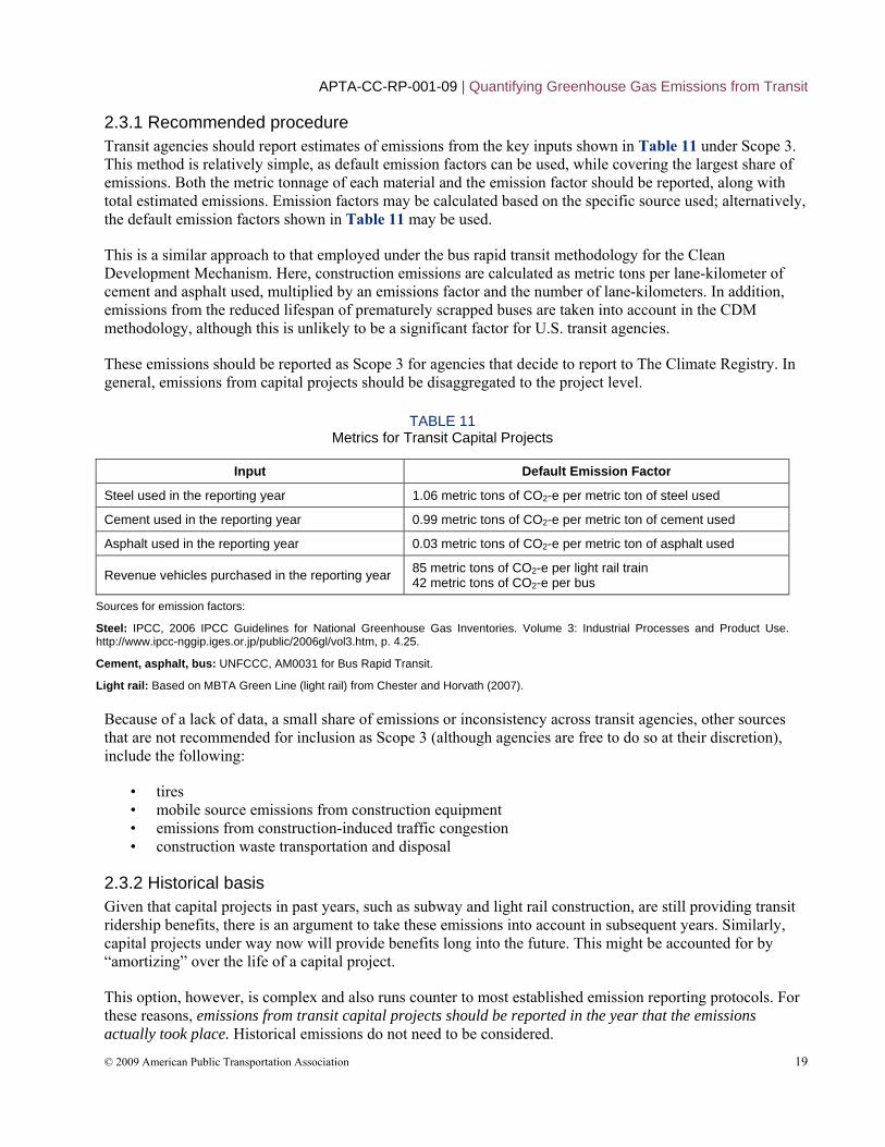
2.3.1 Recommended procedure Transit agencies should report estimates of emissions from the key inputs shown in Table 11 under Scope 3. This method is relatively simple, as default emission factors can be used, while covering the largest share of emissions. Both the metric tonnage of each material and the emission factor should be reported, along with total estimated emissions. Emission factors may be calculated based on the specific source used; alternatively, the default emission factors shown in Table 11 may be used.
This is a similar approach to that employed under the bus rapid transit methodology for the Clean Development Mechanism. Here, construction emissions are calculated as metric tons per lane-kilometer of cement and asphalt used, multiplied by an emissions factor and the number of lane-kilometers. In addition, emissions from the reduced lifespan of prematurely scrapped buses are taken into account in the CDM methodology, although this is unlikely to be a significant factor for U.S. transit agencies.
These emissions should be reported as Scope 3 for agencies that decide to report to The Climate Registry. In general, emissions from capital projects should be disaggregated to the project level.
TABLE 11 Metrics for Transit Capital Projects
Input Default Emission Factor
Steel used in the reporting year 1.06 metric tons of CO2-e per metric ton of steel used
Cement used in the reporting year 0.99 metric tons of CO2-e per metric ton of cement used
Asphalt used in the reporting year 0.03 metric tons of CO2-e per metric ton of asphalt used
Revenue vehicles purchased in the reporting year 85 metric tons of CO2-e per light rail train 42 metric tons of CO2-e per bus
Sources for emission factors:
Steel: IPCC, 2006 IPCC Guidelines for National Greenhouse Gas Inventories. Volume 3: Industrial Processes and Product Use. http://www.ipcc-nggip.iges.or.jp/public/2006gl/vol3.htm, p. 4.25.
Cement, asphalt, bus: UNFCCC, AM0031 for Bus Rapid Transit.
Light rail: Based on MBTA Green Line (light rail) from Chester and Horvath (2007).
Because of a lack of data, a small share of emissions or inconsistency across transit agencies, other sources that are not recommended for inclusion as Scope 3 (although agencies are free to do so at their discretion), include the following:
• tires • mobile source emissions from construction equipment • emissions from construction-induced traffic congestion • construction waste transportation and disposal
2.3.2 Historical basis Given that capital projects in past years, such as subway and light rail construction, are still providing transit ridership benefits, there is an argument to take these emissions into account in subsequent years. Similarly, capital projects under way now will provide benefits long into the future. This might be accounted for by “amortizing” over the life of a capital project.
This option, however, is complex and also runs counter to most established emission reporting protocols. For these reasons, emissions from transit capital projects should be reported in the year that the emissions actually took place. Historical emissions do not need to be considered.
APTA-CC-RP-001-09 | Quantifying Greenhouse Gas Emissions from Transit
© 2009 American Public Transportation Association 20
The exception is in the context of an offset project where emission reductions (“carbon credits”) are sold on the market. In this case, construction emissions may be annualized over the crediting period. This is in keeping with methodological precedent in the Clean Development Mechanism (e.g., Approved Methodology AM0031 for Bus Rapid Transit).
2.3.3 Physical scope Emissions should be reported for dedicated transit facilities only, such as stations, intermodal facilities and physically separated rights-of-way (including resurfacing of a separated right-of-way for exclusive use by bus rapid transit). Emissions from general roadway resurfacing projects, street lighting, etc. should be accounted for in the inventory of the respective local government entity (e.g., a county streets department), based on operational control.
3. Mode shift to transit This section provides guidance on methodologies to calculate the mode shift impacts of transit on greenhouse gas emissions. Together with congestion relief and the land-use multiplier (discussed in the following two sections), mode shift to transit leads to “displaced emissions” as private automobile travel is reduced.
There are three major methodological approaches to estimating the mode shift effect on an agency level: the use of regional travel demand models, evidence from “natural experiments” and applying a mode shift factor to data on transit passenger mileage. This guidance recommends the third approach. However, the first two approaches are discussed briefly for the sake of completeness.
3.1 Regional models This approach uses county or regional travel demand models, typically maintained by metropolitan planning organizations (MPOs). The principle is simple: Remove the transit system from the model and calculate vehicle miles traveled and greenhouse gas emissions.
Regional models allow the complexities of feedback effects to be calculated. These include changes in destinations and trip lengths, as well as mode shift to a range of travel alternatives. There are several problems with this approach, however:
• Regional travel demand models are unlikely to be calibrated to address fundamental changes in transit availability.
• MPOs, where such models are normally housed, vary widely in their technical sophistication and in the availability of staff time to conduct such analyses.
• Some models may not deal well with suppressed trips that follow the elimination of a transit service (particularly important where transit has a social role).
• Results for different agencies may not be comparable, as modeling methodologies vary among regions. These discrepancies may grow as some regions switch to activity-based models.
3.2 Natural experiments The second methodological option takes advantage of “natural experiments” in which the transit system ceases to operate for a period of time. Normally, this would happen through industrial action—e.g., the New York City MTA strike of December 2005, the Los Angeles MTA strike of October/November 2003, or the BART strike of 1997. Other examples include regionwide power outages.
The impacts of some of these strikes have been studied in detail. In Los Angeles, a small increase in traffic cut freeway travel speeds by up to 20 percent (Lo and Hall 2006). However, strikes are unsuitable to provide estimates of transit emissions benefits for several reasons:
APTA-CC-RP-001-09 | Quantifying Greenhouse Gas Emissions from Transit
© 2009 American Public Transpor 21
• They cannot provide consistent data across all U.S. transit agencies. • Short-term adaptations for a strike (e.g., working at home or using taxis) may be infeasible as a
longer-term response. • Some strikes are not complete—some staff may work normally, and other transit service providers in
a region (e.g., the municipal operators in Los Angeles) may be unaffected.
3.3 Calculate mode shift factor The recommended approach is to apply a mode shift factor—the ratio of transit passenger miles to displaced private auto miles—to data on passenger mileage. For example, if an agency reports 1,000,000 passenger miles in a given year to the National Transit Database and calculates a mode shift factor of 0.6, it would estimate displaced mileage at 600,000. This can then be converted to CO2-e using a suitable emissions factor. The mode shift factor does not include changes to trip lengths or transit-induced shifts to walking and biking; these are considered in the land-use multiplier (Section 8).
This approach is relatively robust, does not require sophisticated modeling, and draws on readily available data. A precedent can be found in the bus rapid transit methodology approved under the Clean Development Mechanism.
An estimate of the mode shift factor can be derived from logical inference. For example, it might be assumed that individuals with no driver’s license will not shift to private autos. However, there are few clear-cut cases (e.g., these individuals might obtain a ride from a friend or household member). This suggests that stated choice surveys are the most appropriate measure.
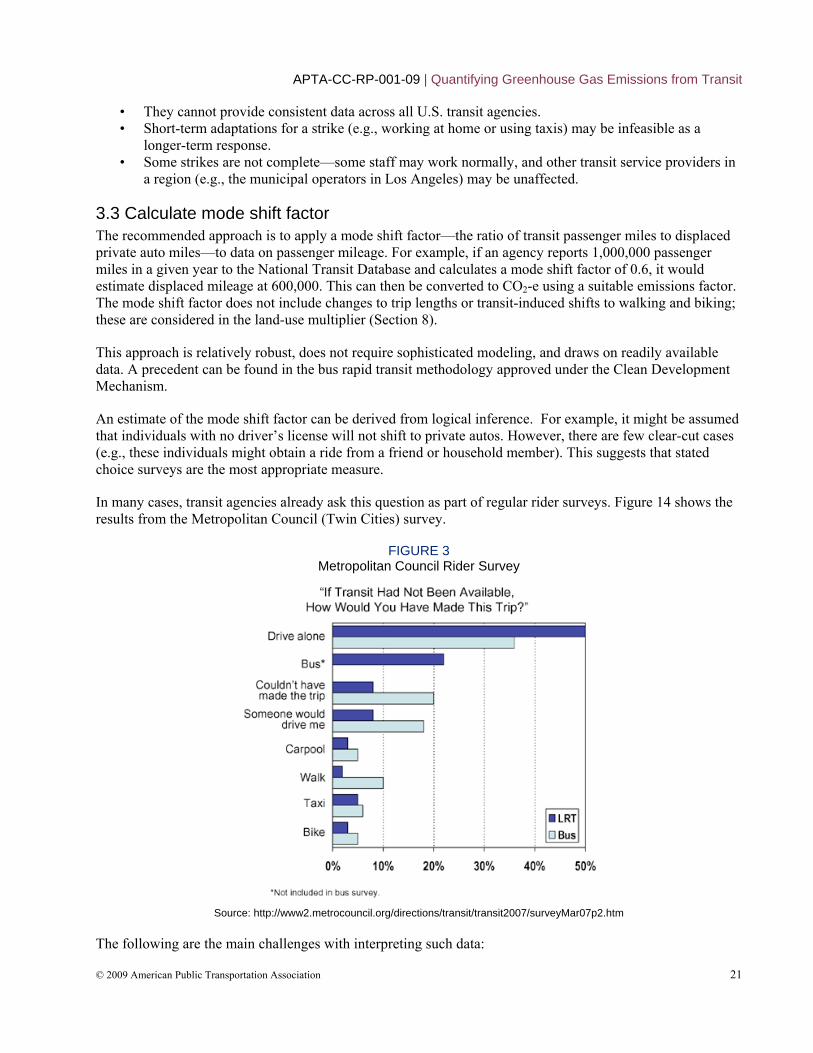
In many cases, transit agencies already ask this question as part of regular rider surveys. Figure 14 shows the results from the Metropolitan Council (Twin Cities) survey.
FIGURE 3 Metropolitan Council Rider Survey
Source: http://www2.metrocouncil.org/directions/transit/transit2007/surveyMar07p2.htm
The following are the main challenges with interpreting such data:
tation Association
APTA-CC-RP-001-09 | Quantifying Greenhouse Gas Emissions from Transit
© 2009 American Public Transportation Association 22
• Long-term responses may differ from short-term (e.g., people might eventually move or purchase a vehicle). An additional question on auto ownership can be used to factor in these longer-term adjustments.
• Methods used to estimate transit passenger miles have some variability among transit agencies. King County Metro Transit, for transit, estimates transit ridership using automatic passenger counting (APC) technologies on a large, stratified sample to estimate unlinked trips and annual passenger miles. Other transit agencies may use other technologies and methods to estimate passenger miles.
• Roadway infrastructure may not be able to accommodate all trips that would shift to private autos, suggesting either that trips may be suppressed or that infrastructure would respond (i.e., highways would be expanded).
• Trip lengths may differ between transit and auto (e.g., if an auto route provides a more direct path). Since individuals generally choose destination and mode simultaneously, trip lengths likely would lengthen in the absence of transit. However, this effect is calculated as part of the land-use multiplier (see Section 8). For purposes of calculating mode shift impacts, equal trip lengths by transit and auto can be assumed.
3.4 Methodological procedure This section provides detailed guidance for a transit agency to calculate its mode shift factor and to estimate its mode shift impact on emissions. It provides different “tiers” to enable agencies to select the most appropriate way to determine a mode shift parameter, based on available data, staff resources and the degree of precision required.
The following procedure should be used.
3.4.1 Step 1: Quantify passenger miles Passenger miles by mode can be found on National Transit Database Form S-10. The assumption is that one passenger mile on transit is equivalent to one passenger mile in a private auto—i.e., that the distances are comparable. Note that while transit may create land-use patterns with overall shorter trip distances, this effect is captured in the land-use multiplier.
3.4.2 Step 2: Calculate mode shift factor Alternative methods for estimating the mode shift factor are described in the next section.
3.4.3 Step 3: Calculate VMT displacement For each mode, multiply passenger miles by the mode shift factor.
3.4.4 Step 4: Estimate average fuel economy for displaced VMT Fuel economy will vary between regions depending on the composition of the vehicle fleet and degree of congestion in each region.
This document presents three methodological approaches to accounting for these regional differences, presenting as tiers in decreasing order of specificity and sophistication:
Tier A: Use a regionally specific factor published by the region’s MPO. MPOs sometimes estimate and publish average speeds for their regions. If it is available from your MPO, use a regionally specific emission factor that accounts for vehicle fleet composition and vehicle speeds. This should be derived from the EPA’s MOVES model.
APTA-CC-RP-001-09 | Quantifying Greenhouse Gas Emissions from Transit
© 2009 American Public Transportation Association 23
Tier B: Use the speed adjustment formula from the Urban Mobility Report. Vehicle speed data for many large urban areas are published in the Texas Transportation Institute’s Urban Mobility Report Appendix A. If using this source, use the weighted average freeway and arterial speed, weighted by VMT. Convert speed to fuel economy with the following formula1:
Average Fuel Economy = 8.8 + (0.25 × Average Speed)
Tier C: Use the national default value for fleet fuel economy from the EPA. If average speed is unavailable, use the conservative 20.2 miles per gallon. Fuel economy data are for light-duty vehicles for the 2006 and 2007 model years, as reported by the EPA, Light-Duty Automotive Technology and Fuel Economy Trends: 1975 Through 2007. Data are for more recent model years, which means that estimates of displaced emissions will be conservative, as older, more inefficient vehicles are not included.
3.4.5 Step 5: Convert to CO2-equivalent If regional or state-specific data are available on emission factors, these may be used. Otherwise, use the following default values:
• CO2 emissions: 8.81 kilograms CO2/gallon of gasoline • N2O emissions: 0.0069 grams N2O/mile and 1 metric ton N2O to 310 metric tons CO2-e • CH4 emissions: 0.0147 grams CH4/mile and 1 metric ton CH4 to 21 metric tons CO2-e
Emission factors are from The Climate Registry General Reporting Protocol v1.0, Tables 13.1 and 13.4.
3.5 Estimating the mode shift factor One of three alternative tiers, in decreasing levels of specificity, may be used to estimate the mode shift factor, which is the ratio between transit passenger miles and displaced private vehicle miles. A mode shift factor of 1.0 indicates that each transit passenger mile displaced one private vehicle mile. In most cases, data will be available in terms of trips rather than miles, but the default assumption is that transit and displaced private vehicle trips are of equal length.
3.5.1 Tier A: Model-based Some larger agencies may have a travel demand model that can be used to estimate the mode shift factor. Note that this is not the same as using a travel demand model to estimate displaced emissions through removing the transit system altogether.
For example, a preliminary, selective analysis for New York MTA quantified the growth in transit trips from 2000 to 2006. The model was then run using the 2006 scenario, but with transit ridership constrained to 2000 levels. This indicates the alternative modes that these new transit riders would have used. While this is a marginal analysis (i.e., new riders only), it is reasonable to apply the same mode shift factor to the entire ridership. Mode shift factors ranged from 0.29 for New York City Transit (reflecting higher density, greater potential for walking and cycling, and low car ownership) to 0.92 for Long Island Bus (reflecting lower density, lesser potential for walking and cycling, and higher car ownership).
For Tier A to be used, the model must include non-motorized trips in its modal options, as many transit trips may otherwise have been made on foot or bicycle, or the results must be post-processed via an off-model analysis to account for non-motorized trips. The model or post-processing must also reflect induced demand—i.e., some transit trips would not have been made at all if transit were not available. The NYMTA
1 This relationship is used in the Texas Transportation Institute’s Urban Mobility Report, and credited originally to Raus, J. A Method for Estimating Fuel Consumption and Vehicle Emissions on Urban Arterials and Networks, Report No. FHWA-TS-81-210, April 1981.
APTA-CC-RP-001-09 | Quantifying Greenhouse Gas Emissions from Transit
© 2009 American Public Transportation Association 24
model addressed this through discounting the change in auto trips and VMT by the proportion of zero-car households in the origin zone. For example, if the original modeling showed a reduction of 10 vehicle trips from a zone with 20 percent zero-car households, a reduction of 10 × (1 – 0.2) = 8 vehicle trips would be estimated.
3.5.2 Tier B: Survey-based Transit agencies often undertake rider surveys that include a question on alternative modes of travel were transit unavailable for that trip. These may be used to estimate the mode shift factor as follows:
Mode shift factor = % stating they would drive alone + % stating that someone else would drive them + % shifting to taxi + % stating they would carpool / average carpool occupancy
If local estimates of average carpool occupancy are unavailable, use a default of 2.5. This is a conservative estimate, assuming a mix of two- and three-person carpools.
A survey must adhere to the following requirements:
• It must include an option for respondents to indicate that they would not make the trip if transit were unavailable, in order to capture induced demand.
• It must be representative of all transit riders and include a maximum 5 percent margin of error with 95 percent confidence (generally, this requires about 375 responses, depending on total ridership). This standard does not prescribe specific sampling techniques. For further information, refer to TCRP Synthesis 63, On-Board and Intercept Transit Survey Techniques (2005).
• The survey must have been conducted within the past five years, in order to capture current land-use and demographic patterns.
Agencies that offer distinct types of service that serve different markets (e.g., bus and commuter rail) may wish to develop specific mode shift factors by mode or market.
The recommended question wording is as follows:
If transit service were not available, how would you make this kind of trip? □ Drive alone □ Walk □ Someone would drive me □ Carpool □ Taxi □ Bicycle □ I would not make this trip
The question wording is from the Transit Performance Monitoring System (TPMS), although the response options have been augmented to distinguish between chauffeur-driven trips (“someone would drive me”) and carpools. Note that this has not yet been pre-tested, a step that should be undertaken before full implementation.
NOTE: The TPMS initiative aimed to standardize the collection of data across agencies, and quantify the performance and benefits of transit service.
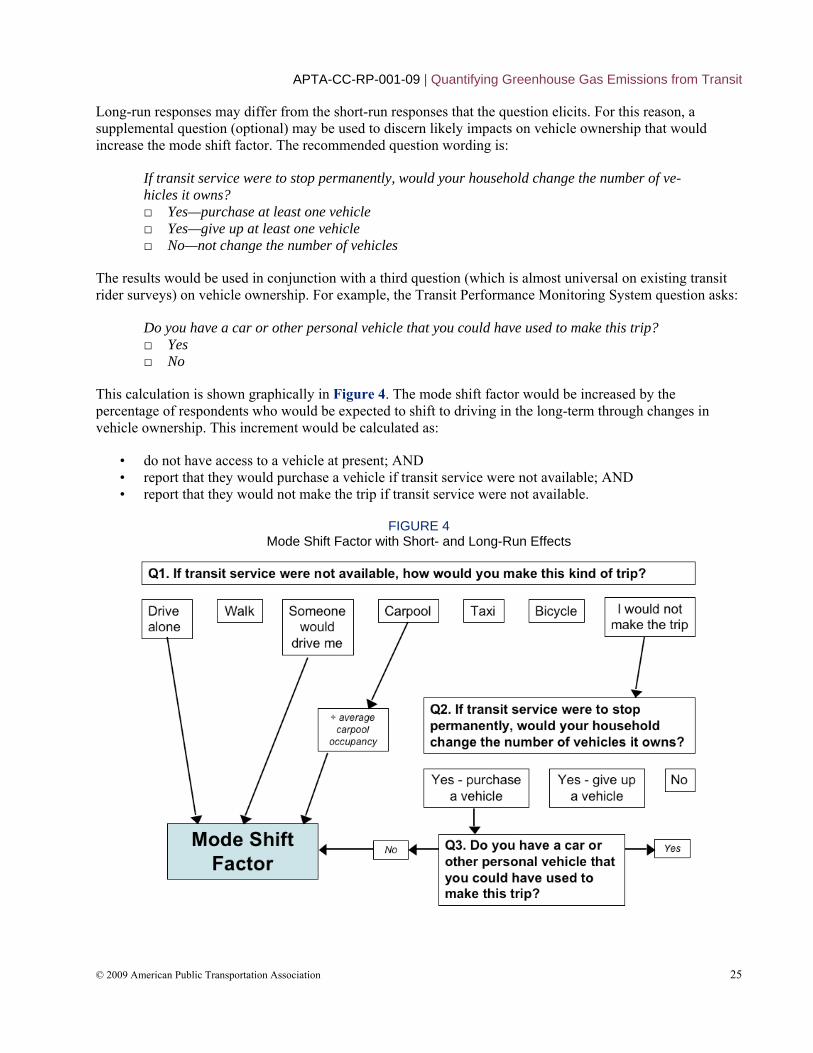
APTA-CC-RP-001-09 | Quantifying Greenhouse Gas Emissions from Transit
© 2009 Am 25
Long-run responses may differ from the short-run responses that the question elicits. For this reason, a supplemental question (optional) may be used to discern likely impacts on vehicle ownership that would increase the mode shift factor. The recommended question wording is:
If transit service were to stop permanently, would your household change the number of ve-hicles it owns? □ Yes—purchase at least one vehicle □ Yes—give up at least one vehicle □ No—not change the number of vehicles
The results would be used in conjunction with a third question (which is almost universal on existing transit rider surveys) on vehicle ownership. For example, the Transit Performance Monitoring System question asks:
Do you have a car or other personal vehicle that you could have used to make this trip? □ Yes □ No
This calculation is shown graphically in Figure 4. The mode shift factor would be increased by the percentage of respondents who would be expected to shift to driving in the long-term through changes in vehicle ownership. This increment would be calculated as:
• do not have access to a vehicle at present; AND • report that they would purchase a vehicle if transit service were not available; AND • report that they would not make the trip if transit service were not available.
FIGURE 4 Mode Shift Factor with Short- and Long-Run Effects
erican Public Transportation Association
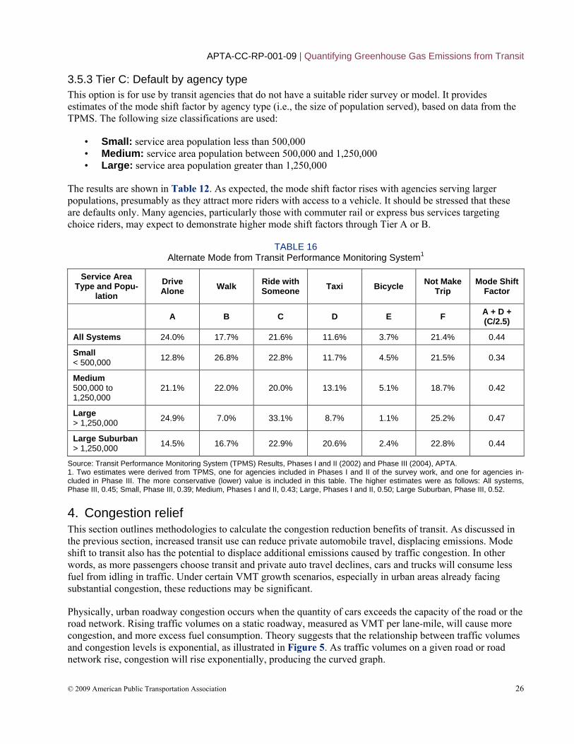
APTA-CC-RP-001-09 | Quantifying Greenhouse Gas Emissions from Transit
© 2009 American Public Transportation Association 26
3.5.3 Tier C: Default by agency type This option is for use by transit agencies that do not have a suitable rider survey or model. It provides estimates of the mode shift factor by agency type (i.e., the size of population served), based on data from the TPMS. The following size classifications are used:
• Small: service area population less than 500,000 • Medium: service area population between 500,000 and 1,250,000 • Large: service area population greater than 1,250,000
The results are shown in Table 12. As expected, the mode shift factor rises with agencies serving larger populations, presumably as they attract more riders with access to a vehicle. It should be stressed that these are defaults only. Many agencies, particularly those with commuter rail or express bus services targeting choice riders, may expect to demonstrate higher mode shift factors through Tier A or B.
TABLE 16 Alternate Mode from Transit Performance Monitoring System1
Service Area Type and Popu-
lation Drive Alone Walk Ride with
Someone Taxi Bicycle Not Make Trip
Mode Shift Factor
A B C D E F A + D + (C/2.5)
All Systems 24.0% 17.7% 21.6% 11.6% 3.7% 21.4% 0.44
Small < 500,000 12.8% 26.8% 22.8% 11.7% 4.5% 21.5% 0.34
Medium 500,000 to 1,250,000
21.1% 22.0% 20.0% 13.1% 5.1% 18.7% 0.42
Large > 1,250,000 24.9% 7.0% 33.1% 8.7% 1.1% 25.2% 0.47
Large Suburban > 1,250,000 14.5% 16.7% 22.9% 20.6% 2.4% 22.8% 0.44
Source: Transit Performance Monitoring System (TPMS) Results, Phases I and II (2002) and Phase III (2004), APTA. 1. Two estimates were derived from TPMS, one for agencies included in Phases I and II of the survey work, and one for agencies in-cluded in Phase III. The more conservative (lower) value is included in this table. The higher estimates were as follows: All systems, Phase III, 0.45; Small, Phase III, 0.39; Medium, Phases I and II, 0.43; Large, Phases I and II, 0.50; Large Suburban, Phase III, 0.52.
4. Congestion relief This section outlines methodologies to calculate the congestion reduction benefits of transit. As discussed in the previous section, increased transit use can reduce private automobile travel, displacing emissions. Mode shift to transit also has the potential to displace additional emissions caused by traffic congestion. In other words, as more passengers choose transit and private auto travel declines, cars and trucks will consume less fuel from idling in traffic. Under certain VMT growth scenarios, especially in urban areas already facing substantial congestion, these reductions may be significant.
Physically, urban roadway congestion occurs when the quantity of cars exceeds the capacity of the road or the road network. Rising traffic volumes on a static roadway, measured as VMT per lane-mile, will cause more congestion, and more excess fuel consumption. Theory suggests that the relationship between traffic volumes and congestion levels is exponential, as illustrated in Figure 5. As traffic volumes on a given road or road network rise, congestion will rise exponentially, producing the curved graph.
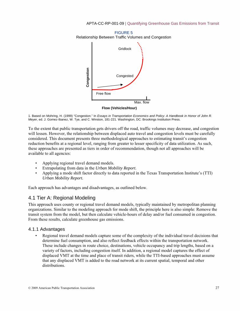
APTA-CC-RP-001-09 | Quantifying Greenhouse Gas Emissions from Transit
© 2009 American Public Transportation Association 27
FIGURE 5 Relationship Between Traffic Volumes and Congestion
Max. flow
Free flow
Congested
Gridlock
Con
gest
ion
Flow (Vehicles/Hour)
1. Based on Mohring, H. (1999) “Congestion.” In Essays in Transportation Economics and Policy: A Handbook in Honor of John R. Meyer, ed. J. Gomez-Ibanez, W. Tye, and C. Winston, 181-221. Washington, DC: Brookings Institution Press.
To the extent that public transportation gets drivers off the road, traffic volumes may decrease, and congestion will lessen. However, the relationship between displaced auto travel and congestion levels must be carefully considered. This document presents three methodological approaches to estimating transit’s congestion reduction benefits at a regional level, ranging from greater to lesser specificity of data utilization. As such, these approaches are presented as tiers in order of recommendation, though not all approaches will be available to all agencies:
• Applying regional travel demand models. • Extrapolating from data in the Urban Mobility Report. • Applying a mode shift factor directly to data reported in the Texas Transportation Institute’s (TTI)
Urban Mobility Report.
Each approach has advantages and disadvantages, as outlined below.
4.1 Tier A: Regional Modeling This approach uses county or regional travel demand models, typically maintained by metropolitan planning organizations. Similar to the modeling approach for mode shift, the principle here is also simple: Remove the transit system from the model, but then calculate vehicle-hours of delay and/or fuel consumed in congestion. From these results, calculate greenhouse gas emissions.
4.1.1 Advantages • Regional travel demand models capture some of the complexity of the individual travel decisions that
determine fuel consumption, and also reflect feedback effects within the transportation network. These include changes in route choice, destinations, vehicle occupancy and trip lengths, based on a variety of factors, including congestion itself. In addition, a regional model captures the effect of displaced VMT at the time and place of transit riders, while the TTI-based approaches must assume that any displaced VMT is added to the road network at its current spatial, temporal and other distributions.
APTA-CC-RP-001-09 | Quantifying Greenhouse Gas Emissions from Transit
© 2009 American Public Transportation Association 28
4.1.2 Disadvantages • Extensive use of a regional travel demand model may require significant staff time and/or resources.
MPOs, where such models are normally housed, vary widely in their technical sophistication and in the availability of staff time to conduct such analyses.
• Regional travel demand models are unlikely to be calibrated to address fundamental changes in transit availability, such as significant increases or decreases in system capacity.
Results for different agencies may not be comparable, as modeling methodologies vary among regions. These discrepancies may grow as some regions switch to activity-based models.
4.2 Tier B: Extrapolating from Urban Mobility Report data This approach extends the data available in the Urban Mobility Report to produce a metropolitan-wide estimate of fuel savings from public transportation service. This approach posits an exponential relationship between traffic density and congestion, as described in Figure 5—that is, as auto VMT per lane-mile in a given region increases, so will congestion levels. Transit agencies can use historical data from the Urban Mobility Report to model this correlation for their regions, estimate the additional auto VMT that would result if public transportation operations were to be discontinued, and produce a new estimate of excess fuel consumption. Comparing this new estimate to the predicted congestion levels at current traffic density isolates the effect of transit.
4.2.1 Step 1: Establish a correlation between traffic density and fuel consumption Approximately 25 years of historical data for a given metropolitan area may be found in complete data tables from the Urban Mobility Report Web site at http://mobility.tamu.edu/ums/congestion_data/tables/ complete_data.xls. In a spreadsheet, establish the following series, over time:
• Auto VMT = Freeway daily vehicle-miles of travel + Arterial daily vehicle-miles of travel • Lane-miles = Freeway lane-miles + Arterial lane-miles • Traffic density = Auto VMT ÷ Lane-miles • Excess fuel consumed in congestion (total gallons)
If local data sources are available, particularly for auto VMT and lane-miles, perhaps from the state Department of Transportation or other source, those alternate data sources should be tested as well. The correlation between traffic density and excess fuel consumption from congestion usually shows an exponential relationship, able to be modeled in a spreadsheet. Typically, this relationship can be expressed as:
Y = α × eβx Where Y is excess fuel consumed in congestion, X is traffic density, α and β are coefficients deter-mined by the statistical relationship between the two data series from TTI (calculated in the spread-sheet), and e is the base of the natural logarithm.
Figure 6 presents an example of this approach using data from the Chicago region, where blue circles are historical TTI data, and the two squares represent predicted excess fuel consumption with and without displaced auto VMT.

APTA-CC-RP-001-09 | Quantifying Greenhouse Gas Emissions from Transit
© 2009 American Public Transportation Association 29
FIGURE 6 Correlation Between Traffic Density and Excess Fuel Consumption
R2 = 0.96-
50
100
150
200
250
1,000 1,500 2,000 2,500 3,000
Exc
ess
Fue
l Con
sum
ed in
C
onge
stio
n (m
illio
n ga
llons
)
Traffic Density (VMT per Lane-Mile)
4.2.2 Step 2: Estimate displaced auto VMT Use the mode shift factor as calculated in the preceding section, and apply to all transit passenger-miles in the region shown in the Urban Mobility Report. To be consistent with the relationship established with TTI data, passenger-miles from all transit service providers in the region should be included. This captures the comprehensive, cumulative effect of transit services in the region.
4.2.3 Step 3: Estimate additional fuel consumption from congestion Add displaced auto VMT to current auto VMT, recalculate traffic density to include this displaced VMT, and then recalculate excess fuel from congestion using the equation established in Step 1. The difference between the fuel consumption predicted with and without this displaced auto VMT represents the fuel congestion benefit of transit.
If using Microsoft Excel, the GROWTH() statistical function may be used to estimate excess fuel consumption with and without displaced auto VMT. In this function, known_y’s are historical excess fuel consumption from congestion, known_x’s are historical traffic densities, and new_x’s are the current with-transit and predicted no-transit traffic densities.
4.2.4 Step 4: Convert fuel savings to displaced emissions Use default emission factors to calculate displaced CO2 emissions, as described in Section 6.4.5 (regionally specific factors can again be substituted, if available). However, unlike in 6.4.5, APTA recommends omitting emissions of N2O and CH4 for this step, since the exact relationship between vehicle congestion and emissions of these pollutants on a per-mile basis is unclear.
4.2.5 Advantages • The primary advantage to this approach is its closer compatibility with the mode shift methodology
previously described, while requiring only moderate effort to complete. When agencies model the effect of discontinuing public transportation, this approach uses the same mode shift factor, ensuring that the resulting congestion benefits can be added to mode shift benefits for a particular region or agency.
APTA-CC-RP-001-09 | Quantifying Greenhouse Gas Emissions from Transit
© 2009 American Public Transportation Association 30
• This approach models the exponential relationship between traffic volumes and congestion levels, which provides a more comprehensive view of the cumulative effect of public transportation services in an urban area.
4.2.6 Disadvantages • First, data is available for only 85 U.S. urban areas, and only at the metropolitan level. Agencies
whose location is not one of the 85 urban areas in the report cannot readily use this approach. Agencies that do not represent all transit service in the metropolitan area will need to make several adjustments to divide metropolitan-level benefits among modes and agencies (see Section 7.2.7 for guidance).
• Second, this approach must also rely on some assumptions, including that transit buses have a minimal effect on congestion now, so that their elimination would have no effect on congestion. This approach also assumes that displaced transit travel would occur at the same time and locations as auto travel (i.e., that displaced transit riders would join the roadway network following the current spatial and temporal distribution of roadway traffic). To the extent that transit trips occur on the most congested corridors during the most congested times of day, this approach is conservative.
NOTE: Transit buses in mixed traffic consume roadway capacity and may contribute to congestion. However, these effects are likely relatively small compared with private auto travel.
• Third, the statistical relationship between traffic density and historical congestion as reported by TTI appears to be weaker in some cities, while quite strong in others. Therefore, APTA recommends using this methodology only if the resulting R-squared value from fitting an exponential line of best fit to this data is above 0.70 (in this case, R-squared is a statistical measure of how well traffic density explains variation in excess fuel consumption). Although the current congestion levels often diverge from predicted congestion in the current year, the difference between the two scenarios is the focus of this approach, as this difference reflects the regionally specific effect of displaced VMT.
• Fourth, this approach may underestimate the congestion impact of public transportation due to simplifying assumptions. The methodology assumes that displaced auto VMT is added to roadways in proportion to existing travel patterns by auto (current occupancy rate, spatial and temporal distribution, etc.), while transit use tends to be high in heavily congested corridors at peak travel times, where congestion relief benefits are also high.
• Finally, this approach is somewhat more complex. However, with some spreadsheet manipulation and moderate effort, agencies can convert published figures into displaced emissions.
4.2.7 Allocation among agencies In some cases, transit providers in a region with multiple agencies may wish to attribute the benefit to a particular agency. In this instance, the following procedure is recommended:
Step 1: Calculate reduction from congestion relief for the metropolitan region.
Step 2: Calculate the share of regional transit unlinked trips provided by a given agency. NTD data for the most recent year should be used.
Step 3: Calculate an individual agency's contribution to congestion relief reductions by multiplying the emissions reductions from congestion relief by the agency’s share of unlinked transit trips.
NOTE: Allocation based on unlinked trips rather than passenger miles is recommended, as agencies serving shorter trips in denser parts of the region will make the greatest contribution to congestion re-lief.
APTA-CC-RP-001-09 | Quantifying Greenhouse Gas Emissions from Transit
© 2009 American Public Transportation Association 31
4.3 Tier C: Using Urban Mobility Report data The Texas Transportation Institute’s Urban Mobility Report, published annually, estimates the additional amount of fuel that would be consumed if public transportation operations were to be discontinued. As the simplest method to calculate transit’s congestion reduction benefits, this fuel use figure can be converted to displaced emissions following The Climate Registry’s Tier B methodology, using several assumptions and a mode shift factor, as detailed below.
The mode shift factor estimated in Section 6.5 should be used to discount the Urban Mobility Report, since TTI calculates private auto fuel savings from public transit using a mode shift factor of 0.8. This assumption implies that that every transit passenger’s next-best alternate mode would be the private automobile at an average vehicle occupancy of 1.25. The mode shift factor estimation in this document, however, incorporates regionally specific information about passengers’ next-best alternate mode, and average vehicle occupancy. To account for differences in mode shift factors between the data sources, TTI’s data should be adjusted.
4.3.1 Step 1: TTI fuel savings data Fuel savings may be found in complete data tables from the Texas Transportation Institute’s Urban Mobility Report website, http://mobility.tamu.edu/ums/congestion_data/tables/ complete_data.xls. The most recent year should be used. TTI has specific data for wasted fuel in 85 cities. These data should be used where applicable. Otherwise, average data are available by population size. All agencies will use the data field titled “Condition if public transportation service were discontinued—wasted fuel increase (1000 gallons),” while agencies not among the 85 cities with specific data provided will also need the data field titled “Public transportation annual unlinked passenger trips (million).”
4.3.2 Step 2: Convert TTI fuel savings to displaced emissions Apply the mode shift factor determined in Section 6 and use default emission factors to calculate displaced CO2 emissions. APTA recommends omitting emissions of N2O and CH4, since the exact relationship between vehicle congestion and emissions of these pollutants on a per-mile basis is unclear.
For agencies covered under one of the 85 cities with specific data, adjust total wasted fuel increase consumed in congestion (identified in Step 1) to account for differences in mode shift factors. TTI’s data should be multiplied by the ratio of the mode shift factor used here and 0.8. For example, if TTI reports excess fuel consumption of 200 gallons and the mode shift factor used here is 0.44, multiply 200 gallons × (0.44 / 0.8) = 110 gallons of excess fuel consumed in congestion.
Agencies not covered under one of the 85 cities with specific data may estimate transit’s fuel savings from congestion on a per-trip basis. These agencies can assume that their transit services save an amount of fuel per transit trip similar to cities of similar size. Locate TTI’s average figures for similarly-sized cities, and divide the total excess fuel consumed in congestion by the TTI public transportation annual unlinked passenger trips (identified in Step 1) to determine a fuel saved per trip. Multiply this fuel saved per trip by the unlinked passenger trips from NTD identified in Section 6, to produce a total fuel saved from transit due to congestion relief for an agency not covered under one of the 85 cities. Again, to account for differences in mode shift factors between TTI and this APTA guidance, multiply this number by the ratio of the mode shift factor used here and 0.8. For example, if this evaluation produces an estimate of excess fuel consumption of 200 gallons, and the mode shift factor used is 0.44, multiply 200 gallons × (0.44 / 0.8) = 110 gallons of excess fuel consumed in congestion.
CO2 emission factors and average fuel economy values should be consistent with whatever is used in calculating mode shift. If available, agencies may use fuel economy data based on regional fleet characteristics. Otherwise, the following default values may be used:
APTA-CC-RP-001-09 | Quantifying Greenhouse Gas Emissions from Transit
© 2009 American Public Transportation Association 32
• CO2 emissions: 8.81 kg CO2/gallon. • Fleet average fuel economy: Apply the results of Section 6.4.4.
NOTE: Emission factor is from The Climate Registry General Reporting Protocol v1.0, Tables 13.1 and 13.4.
4.3.3 Advantages • The primary advantage to this approach is its simplicity. Agencies can convert published figures into
displaced emissions quickly and easily.
4.3.4 Disadvantages • First, agencies that do not represent all transit service in the metropolitan area cannot claim the entire
sum of benefits reported by TTI. A process by which to divide the metropolitan figure among modes or agencies is complex (see Section 7.2.7 for guidance).
• Second, this approach assumes that the TTI’s congestion savings estimation methodology is broadly compatible with the mode shift factor. The Urban Mobility Report calculates congestion based on a relationship between traffic volumes and peak direction speed. This approach is conceptually consistent with displaced auto VMT, but applying a mode shift factor to these results is an approximation.
Quantifying the benefit of congestion relief provided by public transportation can be complex, and the techniques by which this benefit can be measured are being further refined. However, insofar as transit attracts some automobile traffic away from roadways, transit’s effect on congestion levels may be potentially significant.
5. The land-use multiplier This section provides guidance on methodologies to calculate the land-use multiplier for transit impacts on greenhouse gas emissions. Together with mode shift and congestion relief (discussed in the previous two sections), the land-use multiplier leads to “displaced emissions” as private automobile travel is reduced. Unlike the prior two displacement areas, methodologies to measure the land use impacts of transit are evolving and local variables strongly influence how to measure these impacts. For this reason, this section presents as a guideline alternate methodologies and recommends that transit agencies use these methodologies or adapt other methodologies for their local circumstances.
5.1 What is the land-use multiplier? The land-use multiplier accounts for the indirect impacts of transit on reducing vehicle travel. These impacts include the following (Neff 1996; Newman and Kenworthy 1999; Litman 2006):
• Reduced trip lengths. Higher-density development would in many cases not be possible without the existence of transit—for example, due to the need to provide more parking. By facilitating compact development in this way, transit can shrink the footprint of the urban area and reduce overall travel distances. In addition, residents often adjust to the availability of transit by moving closer to bus and rail corridors. This may be partly offset when the transit route structure forces travel by an indirect route, particularly when a suburb-to-suburb trip requires a transfer downtown.
• Facilitation of bicycle and pedestrian travel. As well as reducing trip lengths, the higher densities and mix of uses supported by transit enable mode shift from the private auto to walking and cycling. For example, pedestrian-oriented shops and services may not be economically viable without the density and foot traffic that transit supports.
APTA-CC-RP-001-09 | Quantifying Greenhouse Gas Emissions from Transit
© 2009 American Public Transportation Association 33
• Trip chaining. Transit can facilitate the combination of trips into a single tour. For example, a commuter may pick up groceries or dry cleaning on the way home from the station.
• Impacts through vehicle ownership. Households living close to transit tend to own fewer vehicles, partly because a vehicle may not be needed for commuting, and partly because of the reduced availability and higher cost of parking. In turn, reduced vehicle availability tends to lead to reduced auto use, and the private car may cease to become the habitual choice for every trip.
5.2 Evidence for the land-use multiplier Disentangling these cause-and-effect relationships between transit and land use is a substantial methodological challenge. Some of the approaches taken, summarized in Table 17, include the following:
• Correlation of transit and auto travel. These studies, beginning with Pushkarev and Zupan (1982), use the empirical observation that cities with high public transit use show far lower rates of auto travel than would be implied by the direct substitution of auto with transit trips. In a study of 32 global cities, Newman and Kenworthy (1999) estimate a land-use multiplier of between 5 and 7, meaning that for every extra passenger mile on transit per capita, vehicle miles per capita decline by five to seven miles. Holtzclaw (2000) compares three prototypical cities in the San Francisco Bay Area (San Francisco, Walnut Creek and San Ramon), and computes a reduction in vehicle travel of between 1.4 and 9 for every mile of transit passenger travel. More recent, as-yet-unpublished work by Newman, Kenworthy and Glazebrook identifies an exponential relationship between transit and auto travel: As the use of public transport increases linearly, auto travel decreases exponentially.
• Travel time budget analysis. Neff (1996) uses travel time budget theory to analyze the substitution of transit travel for auto travel in U.S. urbanized areas. He concludes that every mile of transit travel replaces 5.4 to 7.5 miles of auto travel.
• Structural equations modeling. The most recent and sophisticated study, by ICF International for APTA, uses National Household Travel Survey data and structural equations modeling (SEM) (a complex form of analysis used to assess correlations between multiple variables) to disentangle the causal relationships (Bailey, Mokhtarian et al. 2008). In contrast to earlier studies, which mainly identify correlations between auto and transit travel, SEM can help explain the extent to which transit causes denser, more walkable land-use patterns, and conversely the extent to which these land-use patterns create a need for improved transit service. This ICF study concludes (p. 12) that “the magnitude of the secondary effect is approximately twice as large as the primary effect of actual public transit trips,” giving a multiplier of 1.9. Another finding (p. 1) is of “a significant correlation between transit availability and reduced automobile travel, independent of transit use.” However, the complexities of SEM as a technique, the inability of SEM-based analysis to prove or disprove relationships, and the low variance seen for many variables make it difficult to know how best to interpret the findings of the this analysis for an individual city. Furthermore, the fact that the study compared U.S. cities without transit to those that have transit may reduce the overall impact of transit due to the enormous variation in city geography and climate conditions and the highly skewed nature of transit in the United States (i.e., a few cities account for most of the public transit in the United States).
• Mixed comparative approach. The New York Metropolitan Transportation Authority (MTA) has used several methodologies, including four-step modeling, land use comparisons, and travel behavior analysis to estimate the land use impacts of transit. These studies produce a wide range of impacts depending on the area being evaluated and the method. The results from the MTA analysis are presented in an appendix to this document, and range from 1.29 to 6.34.
Evidence for the land-use multiplier is considerably strengthened by the fact that these studies generally show an impact in the same direction and order of magnitude. This is despite significant differences in methodologies, geographic context and the method of computing the multiplier (some studies report it as the
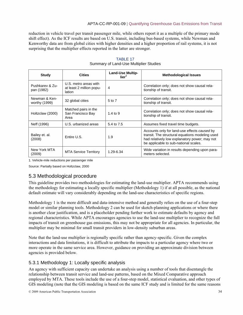
APTA-CC-RP-001-09 | Quantifying Greenhouse Gas Emissions from Transit
© 2009 American Public Transportation Association 34
reduction in vehicle travel per transit passenger mile, while others report it as a multiple of the primary mode shift effect). As the ICF results are based on U.S. transit, including bus-based systems, while Newman and Kenworthy data are from global cities with higher densities and a higher proportion of rail systems, it is not surprising that the multiplier effects reported in the latter are stronger.
TABLE 17 Summary of Land-Use Multiplier Studies
Study Cities Land-Use Multip-lier1 Methodological Issues
Pushkarev & Zu-pan (1982)
U.S. metro areas with at least 2 million popu-lation
4 Correlation only; does not show causal rela-tionship of transit.
Newman & Ken-worthy (1999) 32 global cities 5 to 7 Correlation only; does not show causal rela-
tionship of transit.
Holtzclaw (2000) Matched pairs in the San Francisco Bay Area
1.4 to 9 Correlation only; does not show causal rela-tionship of transit.
Neff (1996) U.S. urbanized areas 5.4 to 7.5 Assumes fixed travel time budgets.
Bailey et. al. (2008) Entire U.S. 1.9
Accounts only for land-use effects caused by transit. The structural equations modeling used had relatively low explanatory power; may not be applicable to sub-national scales.
New York MTA (2009) MTA Service Territory 1.29-6.34 Wide variation in results depending upon para-
meters selected.
1. Vehicle-mile reductions per passenger mile
Source: Partially based on Holtzclaw, 2000
5.3 Methodological procedure This guideline provides two methodologies for estimating the land-use multiplier. APTA recommends using the methodology for estimating a locally specific multiplier (Methodology 1) if at all possible, as the national default estimate will vary considerably depending on the land-use characteristics of specific regions.
Methodology 1 is the more difficult and data-intensive method and generally relies on the use of a four-step model or similar planning tools. Methodology 2 can be used for sketch-planning applications or where there is another clear justification, and is a placeholder pending further work to estimate defaults by agency and regional characteristics. While APTA encourages agencies to use the land-use multiplier to recognize the full impacts of transit on greenhouse gas emissions, this may not be appropriate for all agencies. In particular, the multiplier may be minimal for small transit providers in low-density suburban areas.
Note that the land-use multiplier is regionally specific rather than agency-specific. Given the complex interactions and data limitations, it is difficult to attribute the impacts to a particular agency where two or more operate in the same service area. However, guidance on providing an approximate division between agencies is provided below.
5.3.1 Methodology 1: Locally specific analysis An agency with sufficient capacity can undertake an analysis using a number of tools that disentangle the relationship between transit service and land-use patterns, based on the Mixed Comparative approach employed by MTA. These tools include the use of a four-step model, statistical evaluation, and other types of GIS modeling (note that the GIS modeling is based on the same ICF study and is limited for the same reasons
APTA-CC-RP-001-09 | Quantifying Greenhouse Gas Emissions from Transit
© 2009 American Public Transportation Association 35
discussed above). This approach is explained in Appendix B and can be adapted to local areas with some modifications.
5.3.2 Methodology 2: Default approach using national data An agency without the capacity to run a regional study as described in Methodology 1 may use the national default multiplier of 1.9 calculated by the ICF study (Bailey et al., 2008). This approach should be used only for sketch-planning applications or where there is another clear justification. This default should be considered a placeholder, pending future work to develop default emission factors that are disaggregated by size and type of region and transit system (for example, through further structural equation modeling work or a Delphi panel of expert opinions).
The calculation is as follows:
Emission reductions from land-use multiplier (metric tons per year) = Transit passenger miles / average vehicle occupancy (default 1.39)
× Emissions per vehicle mile (default 0.436 kg) × 1.9 / 1000
The ICF study uses an average vehicle occupancy figure of 1.39, based on the National Household Travel Survey. Agencies should consult the latest version of the National Household Travel Survey to obtain more up-to-date data and/or state or county data contained in the Survey. Regionally specific figures may be used if available from a regional household survey or similar source, provided that all trips (not just commuter trips) are included. Refer to Section 6 for a discussion of alternatives to the default emission factor. Multiplication by 1.9 represents the land-use multiplier and division by 1000 converts from kilograms to metric tons. Since Methodology 2 is based on NTD passenger mileage figures, these estimates are agency-specific.
5.4 Caveats and next steps • The proposed Methodology 1 is a good basis for estimating GHG emissions, but
additional work is needed to define key parameters: The use of Methodology 1 to estimate GHG impacts provides a solid foundation for estimating GHG impacts. However, MTA’s analysis shows that there is ambiguity in how key parameters (e.g., land use characterization, boundaries for high density and low density areas) should be estimated, primarily resulting from the lack of available data at levels that would allow a more accurate analysis. APTA proposes that additional work be done to develop a standard method for estimating these parameters, and more guidance needs to be provided on how to define data inputs.
• Land use multipliers are highly sensitive to assumption: MTA’s analyses showed that land use impacts are highly sensitive to assumption. APTA believes that guidance needs to be developed to define a standard approach to defining areas and identifying comparison groups.
• Land use analysis is more applicable to small areas than large areas: Land use varies greatly within large areas. Because of this, it is difficult to make generalizations about land use within a large area. APTA recommends that future analyses attempt to conduct a more micro-scale analysis of land use in order to better capture its impacts on public transit.
APTA-CC-RP-001-09 | Quantifying Greenhouse Gas Emissions from Transit
© 2009 American Public Transportation Association 36
Appendix A: Summary of NTD audit procedures The National Transit Database (NTD) program is required by statute. Every FTA formula grant recipient must report to the NTD. Without an annual NTD submission, FTA grant funds are cut off. The response rate is about 100 percent. Data for tiny systems in urban areas and small systems in nonurban (rural) areas are not included in the NTD.
After the close of their local fiscal year, transit authorities produce annual reports, summarizing operating, fleet, and financial data. Under federal requirements, financial reports must be audited. The data are also certified. The data in these reports are entered on to forms on a diskette submitted to the NTD. The data on this diskette must conform to the precise data definitions in the Reporting Manual for the NTD and the Uniform System of Accounts for the NTD.
Sampling error Sampling errors produce faulty estimates. In the NTD, other than passenger miles, annual data is actual data, not a sample estimate. For passenger miles, FTA details specific random sampling procedures and requires a precision of +/- 10 percent at the 95 percent confidence level.
Nonsampling Errors Nonentry error or missing data: Fields that are left blank are returned to the transit agency, along with a detailed review letter highlighting errors and omissions. However, a small percentage, less than 1 percent, of data is missing. Tiny transit authorities, with fewer than 10 vehicles, are exempt from having to complete certain forms. This could produce a nonentry on certain data elements for about 30 tiny systems. On a few occasions, a few months of operating data, not vehicle data, are lost when contractors are changed.
Duplicate entry error: The NTD program requires that services purchased by a transit authority be reported separately from directly operated service. This avoids the double counting problem. The data audit and certification requirements also help avoid redundancy. Few bus fleet reports involve more than one transit authority, reducing the chance for double counting.
Response/measurement error and coding errors: Measurement errors occur when incorrect data is provided. Coding errors occur when correct data is improperly recorded. NTD staff work hard to catch bad data and recording errors. First, transit authorities file NTD reports each year; the NTD is not a special study. Regular reporting reduces errors. Second, the data is audited and certified by local officials. Third, FTA validation analysts, familiar with this transit authority, use range checks for 1999 data against data from last year and previous years. Data fields are also checked for proper coding. Validation is discussed, below. Fourth, validation ratios and performance measures, such as operating costs per vehicle, vehicle miles per trip, are calculated. These ratios are compared to previous submissions and systems of similar size. Any significant variations are flagged and returned to the transit authority to explain or revise. This validation feedback loop is very important in producing accurate data for legislative apportionments is not a common feature of most industry databases run by the government.
Verification and validation To produce an accurate and equitable apportionment of FTA funds across the nation, the FTA has made a commitment of significant resources in its NTD detailed verification and validation feedback process. Intensive data validation efforts are not a common feature of most industry databases run by the government. In most industry databases, data is usually accepted as submitted. The NTD employs a number of exhaustive verification and validation efforts. First, transit authorities file NTD reports each year; the NTD is not a special study. Regular reporting increases consistency and reduces errors. Second, at the local transit level, the NTD diskette contains certain error checks. Third, prior to submission, the data is audited and certified. An

APTA-CC-RP-001-09 | Quantifying Greenhouse Gas Emissions from Transit
© 2009 American Public Transportation Association 37
independent auditor must complete an A-128 audit and signs off on the NTD submission. The agency’s CEO certifies the submission. Fourth, FTA validation contractors, familiar with this transit authority, use range checks for 1999 data against data from last year and previous years. Data fields are also checked for proper coding. Errors and inconsistencies are enumerated in a detailed review letter (DRL) that is sent back to the submitting transit agency. DRL problems must be addressed and data revisions made for inclusion in the NTD. Failure to address validation or certification problems can result in loss of eligibility for FTA grants. Fifth, validation ratios and performance measures, such as costs per hour, miles per hour, are calculated. These ratios are compared to previous submissions and systems of similar size. These ratios check the internal consistency of the submission. Any significant inconsistencies are flagged and returned to the transit authority to explain or revise. The NTD contractor performs validation checks involving 200 calculations on each submission. This validation feedback loop is very important in producing accurate data for legislative apportionments and fixed-guideway allocations.
Source: http://www.bts.gov/programs/statistical_policy_and_research/source_and_accuracy_compendium/national_transit_accessibility.html For full details, see http://www.ntdprogram.gov/ntdprogram/reference.htm.
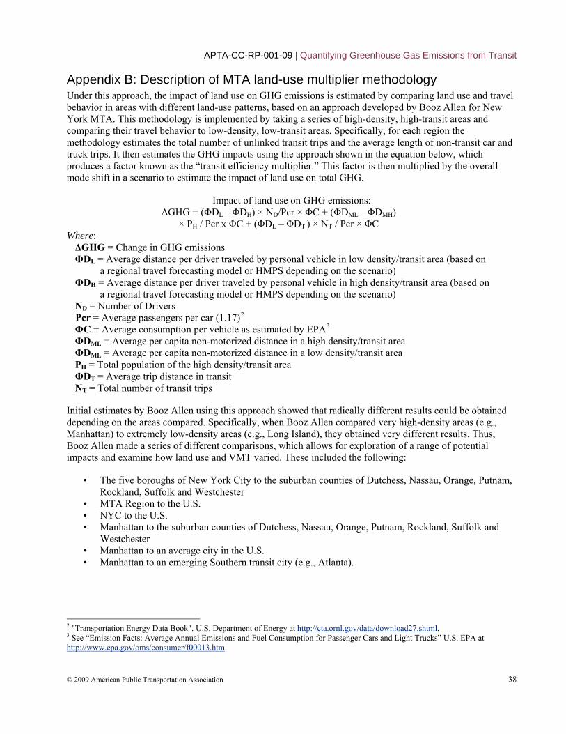
APTA-CC-RP-001-09 | Quantifying Greenhouse Gas Emissions from Transit
© 2009 American Public Transportation Association 38
Appendix B: Description of MTA land-use multiplier methodology Under this approach, the impact of land use on GHG emissions is estimated by comparing land use and travel behavior in areas with different land-use patterns, based on an approach developed by Booz Allen for New York MTA. This methodology is implemented by taking a series of high-density, high-transit areas and comparing their travel behavior to low-density, low-transit areas. Specifically, for each region the methodology estimates the total number of unlinked transit trips and the average length of non-transit car and truck trips. It then estimates the GHG impacts using the approach shown in the equation below, which produces a factor known as the “transit efficiency multiplier.” This factor is then multiplied by the overall mode shift in a scenario to estimate the impact of land use on total GHG.
Impact of land use on GHG emissions: ΔGHG = (ΦDL – ΦDH) × ND/Pcr × ΦC + (ΦDML – ΦDMH)
× PH / Pcr x ΦC + (ΦDL – ΦDT ) × NT / Pcr × ΦC Where: ΔGHG = Change in GHG emissions ΦDL = Average distance per driver traveled by personal vehicle in low density/transit area (based on
a regional travel forecasting model or HMPS depending on the scenario) ΦDH = Average distance per driver traveled by personal vehicle in high density/transit area (based on
a regional travel forecasting model or HMPS depending on the scenario) ND = Number of Drivers Pcr = Average passengers per car (1.17)2 ΦC = Average consumption per vehicle as estimated by EPA3 ΦDML = Average per capita non-motorized distance in a high density/transit area ΦDML = Average per capita non-motorized distance in a low density/transit area PH = Total population of the high density/transit area ΦDT = Average trip distance in transit NT = Total number of transit trips
Initial estimates by Booz Allen using this approach showed that radically different results could be obtained depending on the areas compared. Specifically, when Booz Allen compared very high-density areas (e.g., Manhattan) to extremely low-density areas (e.g., Long Island), they obtained very different results. Thus, Booz Allen made a series of different comparisons, which allows for exploration of a range of potential impacts and examine how land use and VMT varied. These included the following:
• The five boroughs of New York City to the suburban counties of Dutchess, Nassau, Orange, Putnam, Rockland, Suffolk and Westchester
• MTA Region to the U.S. • NYC to the U.S. • Manhattan to the suburban counties of Dutchess, Nassau, Orange, Putnam, Rockland, Suffolk and
Westchester • Manhattan to an average city in the U.S. • Manhattan to an emerging Southern transit city (e.g., Atlanta).
2 "Transportation Energy Data Book". U.S. Department of Energy at http://cta.ornl.gov/data/download27.shtml. 3 See “Emission Facts: Average Annual Emissions and Fuel Consumption for Passenger Cars and Light Trucks” U.S. EPA at http://www.epa.gov/oms/consumer/f00013.htm.
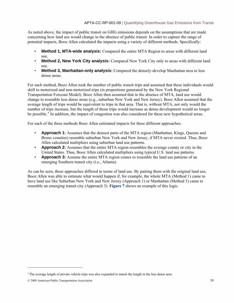
APTA-CC-RP-001-09 | Quantifying Greenhouse Gas Emissions from Transit
© 2009 American Public Transportation Association 39
As noted above, the impact of public transit on GHG emissions depends on the assumptions that are made concerning how land use would change in the absence of public transit. In order to capture the range of potential impacts, Booz Allen calculated the impacts using a variety of different methods. Specifically:
• Method 1, MTA-wide analysis: Compared the entire MTA Region to areas with different land use.
• Method 2, New York City analysis: Compared New York City only to areas with different land use.
• Method 3, Manhattan-only analysis: Compared the densely-develop Manhattan area to less dense areas.
For each method, Booz Allen took the number of public transit trips and assumed that these individuals would shift to motorized and non-motorized trips (in proportions generated by the New York Regional Transportation Forecast Model). Booz Allen then assumed that in the absence of MTA, land use would change to resemble less dense areas (e.g., suburban New York and New Jersey). Booz Allen assumed that the average length of trips would be equivalent to trips in that area. That is, without MTA, not only would the number of trips increase, but the length of those trips would increase as dense development would no longer be possible.4 In addition, the impact of congestion was also considered for these new hypothetical areas.
For each of the three methods Booz Allen estimated impacts for three different approaches:
• Approach 1: Assumes that the densest parts of the MTA region (Manhattan, Kings, Queens and Bronx counties) resemble suburban New York and New Jersey, if MTA never existed. Thus, Booz Allen calculated multipliers using suburban land use patterns.
• Approach 2: Assumes that the entire MTA region resembles the average county or city in the United States. Thus, Booz Allen calculated multipliers using typical U.S. land use patterns.
• Approach 3: Assume the entire MTA region comes to resemble the land use patterns of an emerging Southern transit city (i.e., Atlanta).
As can be seen, these approaches differed in terms of land use. By pairing them with the original land use, Booz Allen was able to estimate what would happen if, for example, the whole MTA (Method 1) came to have land use like Suburban New York and New Jersey (Approach 1) or Manhattan (Method 3) came to resemble an emerging transit city (Approach 3). Figure 7 shows an example of this logic.
4 The average length of private vehicle trips was also expanded to match the length in the less dense area.
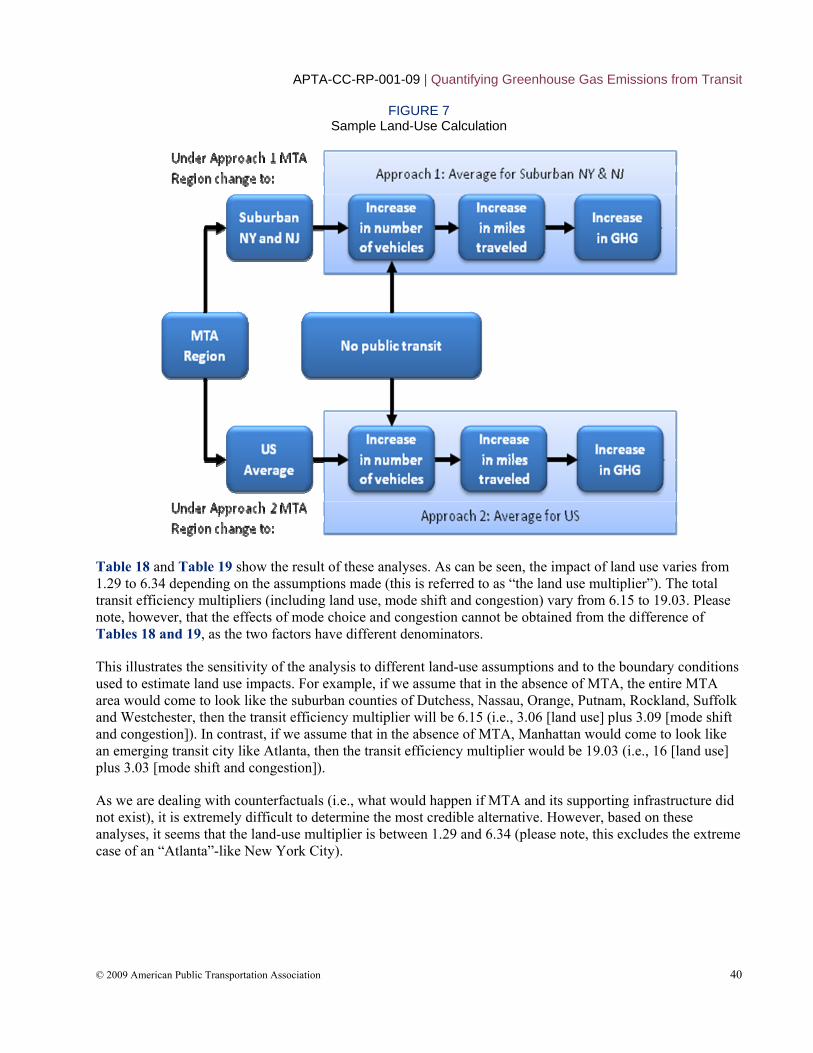
APTA-CC-RP-001-09 | Quantifying Greenhouse Gas Emissions from Transit
© 2009 American Public Transportation Association 40
FIGURE 7 Sample Land-Use Calculation
Table 18 and Table 19 show the result of these analyses. As can be seen, the impact of land use varies from 1.29 to 6.34 depending on the assumptions made (this is referred to as “the land use multiplier”). The total transit efficiency multipliers (including land use, mode shift and congestion) vary from 6.15 to 19.03. Please note, however, that the effects of mode choice and congestion cannot be obtained from the difference of Tables 18 and 19, as the two factors have different denominators.
This illustrates the sensitivity of the analysis to different land-use assumptions and to the boundary conditions used to estimate land use impacts. For example, if we assume that in the absence of MTA, the entire MTA area would come to look like the suburban counties of Dutchess, Nassau, Orange, Putnam, Rockland, Suffolk and Westchester, then the transit efficiency multiplier will be 6.15 (i.e., 3.06 [land use] plus 3.09 [mode shift and congestion]). In contrast, if we assume that in the absence of MTA, Manhattan would come to look like an emerging transit city like Atlanta, then the transit efficiency multiplier would be 19.03 (i.e., 16 [land use] plus 3.03 [mode shift and congestion]).
As we are dealing with counterfactuals (i.e., what would happen if MTA and its supporting infrastructure did not exist), it is extremely difficult to determine the most credible alternative. However, based on these analyses, it seems that the land-use multiplier is between 1.29 and 6.34 (please note, this excludes the extreme case of an “Atlanta”-like New York City).
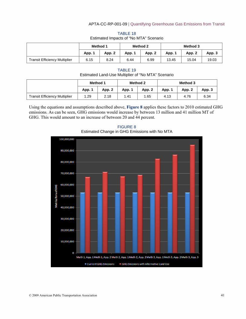
APTA-CC-RP-001-09 | Quantifying Greenhouse Gas Emissions from Transit
© 2009 American Public Transportation Association 41
TABLE 18 Estimated Impacts of “No MTA” Scenario
Method 1 Method 2 Method 3
App. 1 App. 2 App. 1 App. 2 App. 1 App. 2 App. 3
Transit Efficiency Multiplier 6.15 8.24 6.44 6.99 13.45 15.04 19.03
TABLE 19 Estimated Land-Use Multiplier of “No MTA” Scenario
Method 1 Method 2 Method 3
App. 1 App. 2 App. 1 App. 2 App. 1 App. 2 App. 3
Transit Efficiency Multiplier 1.29 2.18 1.41 1.65 4.13 4.76 6.34 Using the equations and assumptions described above, Figure 8 applies these factors to 2010 estimated GHG emissions. As can be seen, GHG emissions would increase by between 13 million and 41 million MT of GHG. This would amount to an increase of between 20 and 44 percent.
FIGURE 8 Estimated Change in GHG Emissions with No MTA
APTA-CC-RP-001-09 | Quantifying Greenhouse Gas Emissions from Transit
© 2009 American Public Transportation Association 42
References Bailey, L. (2007). Public Transportation and Petroleum Savings in the U.S.: Reducing Dependence on Oil
Fairfax, VA, Prepared for American Public Transportation Association by ICF International.
Bailey, L., P.L. Mokhtarian, et al. (2008). The Broader Connection between Public Transportation, Energy Conservation and Greenhouse Gas Reduction. Fairfax, ICF International.
Baxandall, P., T. Dutzik, et al. (2008). A Better Way to Go. Meeting America’s 21st Century Transportation Challenges with Modern Public Transit, CALPIRG Education Fund.
Brown, M. A., F. Southworth, et al. (2008). Shrinking the Carbon Footprint of Metropolitan America, Brookings Institution.
Chester, M. and A. Horvath (2007). Environmental life-cycle assessment of passenger transportation: a detailed methodology for energy, greenhouse gas, and criteria pollutant inventories of automobiles, buses, light rail, heavy rail and air. Berkeley, Calif., Institute of Transportation Studies University of California: 118.
Davis, T. and M. Hale (2007). Public Transportation's Contribution to U.S. Greenhouse Gas Reduction. SAIC, McLean, Virginia, Report for American Public Transportation Association and Transportation Research Board.
Ewing, R., K. Bartholomew, et al. (2008). Growing Cooler: The Evidence on Urban Development and Climate Change. Urban Land Institute, Urban Land Institute.
Feigon, S., D. Hoyt, et al. (2003). Travel Matters: mitigating climate change with sustainable surface transportation. Washington, D.C., Transportation Research Board.
Grütter, J. M. (2007). The CDM in the Transport Sector. Sustainable Transport: A Sourcebook for Policy-makers in Developing Cities. Eschborn, Deutsche Gesellschaft für Technische Zusammenarbeit (GTZ).
Holtzclaw, J. (2000). Does A Mile In A Car Equal A Mile On A Train? Exploring Public Transit's Effectiveness In Reducing Driving.
Litman, T. (2006). Rail Transit In America. A Comprehensive Evaluation of Benefits. Victoria, Victoria Transport Policy Institute.
Lo, S.-C. and R. W. Hall (2006). "Effects of the Los Angeles transit strike on highway congestion." Transportation Research Part A: Policy and Practice 40(10): 903-917.
Neff, J. W. (1996). Substitution Rates Between Transit and Automobile Travel. Association of American Geographers Annual Meeting. Charlotte, NC.
Newman, P. and J. R. Kenworthy (1999). Sustainability and Cities: Overcoming Automobile Dependence. Washington, D.C., Island Press.
Pushkarev, B. S., J. M. Zupan, et al. (1982). Urban Rail in America: An Exploration of Criteria for Fixed-Guideway Transit, Indiana University Press.
Shapiro, R. J., K. A. Hassett, et al. (2002). Conserving Energy and Preserving the Environment: The Role of Public Transportation, Report for American Public Transportation Association.
The Climate Registry (2008). General Reporting Protocol. Version 1.0. Los Angeles, The Climate Registry.
World Resources Institute (2004). The Greenhouse Gas Protocol. A Corporate Accounting and Reporting Standard. Revised Edition., World Resources Institute.
APTA-CC-RP-001-09 | Quantifying Greenhouse Gas Emissions from Transit
© 2009 American Public Transportation Association 43
Definitions AB32: California’s Global Warming Solutions Act of 2006, which includes a binding target to reduce greenhouse gas emissions to 1990 levels by 2020—a reduction of about 25 percent. AB32 also allows the California Air Resources Board to implement a cap-and-trade program to help achieve this goal.
additionality: A measure of whether an offset would have been implemented in the normal course of business. Refers to reductions that are “additional” to the baseline scenario and thus would not have happened but for the offset program. The offset-crediting mechanism does not need to be the only reason for a project to go forward, but it should be a decisive reason.
allowance (or permit): The right to emit one metric ton of CO2-equivalent under a cap-and-trade program. Allowances are traded on carbon markets. Electricity generators and other entities covered under a cap-and-trade program must surrender one allowance for each unit of emissions.
California Climate Action Registry (CCAR): An entity that allows organizations to quantify and register their emissions, providing them with a third-party certified baseline against which any future emission reduction requirements can be measured. In this way, organizations may be able to gain credit for “early actions” they take to reduce emissions in advance of a mandate. CCAR also develops a range of protocols to quantify emissions from an organization or from specific projects. It was established under California statute, and as such is a quasi-governmental nonprofit organization.
cap-and-trade program: A program that limits the amount of a given pollutant that can be emitted into the environment. It is characterized by a fixed number of allowances (the cap, which ensures that a given emissions target is met) and a trading mechanism that allows polluters to buy and sell permits.
carbon “credit”: see offset.
carbon trading: Can refer to a cap-and-trade program for greenhouse gases, or the sale and purchase of greenhouse gas offsets.
Certified Emission Reduction (CER): One unit of greenhouse gas reductions (one metric ton of CO2-equivalent) certified under the Clean Development Mechanism.
Chicago Climate Exchange (CCX): A private organization that provides a trading system for greenhouse gas allowances and offsets. Members make a voluntary but legally binding commitment to reduce their emissions by specified percentages. Any emissions in excess of these requirements can be sold on the exchange, or held in reserve for future years. Members that fall short must purchase additional allowances, which are sold by overperforming members or generated by offset providers. CCX also develops its own protocols for quantifying emission reductions from offset projects.
Clean Development Mechanism (CDM): An offset program established under the Kyoto Protocol. It allows developing countries to participate in greenhouse gas reduction efforts and reduces the costs of Kyoto compliance to industrialized countries. These industrialized countries can achieve their mandated Kyoto targets through a combination of domestic reductions and purchase of Certified Emission Reductions (CERs) from projects in developing nations. CERs also can be purchased by electricity generators and other emitters in Europe, as a way to fulfill their obligations under the European Emissions Trading Scheme. In other words, the two types of allowances are fungible on the European market.
CO2-equivalent (CO2-e): One unit of greenhouse gas emissions standardized by relative global warming potential (usually measured over a 100-year period). Methane, for example, is 21 times more powerful than carbon dioxide, and so one-twenty-first of a metric ton of methane is one metric ton of CO2-e.
[European] Emissions Trading Scheme (ETS): The cap-and-trade program in the European Union.
APTA-CC-RP-001-09 | Quantifying Greenhouse Gas Emissions from Transit
© 2009 American Public Transportation Association 44
global warming potential (GWP): A relative scale that measures how much a given mass of gas is expected to contribute to global warming. Methane, for example, is 21 times more powerful than carbon dioxide, and has a GWP of 21.
land-use multiplier: A factor that accounts for the indirect impacts of transit on reducing vehicle travel, including reduced trip lengths, facilitation of bicycle and pedestrian travel, trip chaining and reduced vehicle ownership.
leakage: Changes in emissions that occur outside of the boundary of the cap-and-trade program or offset project. Leakage can be either positive or negative. Examples might include a reduction in gasoline life-cycle emissions from extracting, transporting and refining oil; induced traffic from a reduction in congestion; or construction emissions.
mode shift factor: The ratio of transit passenger miles to displaced private auto miles.
National Transit Database: A database on transit ridership, energy use, finances and other information, based on data provided by transit agencies and compiled and validated by the Federal Transit Administration. See www.ntdprogram.gov.
offset: A voluntary reduction in emissions from a source that is not covered by a cap-and-trade program. Offsets can include transportation projects (e.g., fuel switching or bus rapid transit); forestry and other biological carbon “sinks”; or destruction of non-CO2 greenhouse gases such as methane or hydrofluorocarbons. Offsets under the Clean Development Mechanism can be used by nations to meet their obligations under the Kyoto Protocol, and by firms under the European Emissions Trading Scheme. Other offsets are voluntary, generating Verified Emission Reductions, and are purchased by organizations for purposes of marketing or corporate social responsibility, or by individuals wishing to reduce their carbon footprint.
permanence: The concept of whether an emissions reduction is permanent—i.e., whether carbon sequestered in soils, forests or underground storage is re-released into the atmosphere. Any emissions reduction in the transportation sector will be permanent (the emissions are not stored, but simply not released), although the years of effectiveness of a project may vary.
protocol (or methodology): The procedure for calculating emission reductions from a specific type of project (e.g., bus rapid transit) or quantifying emissions from a specific type of organization.
Regional Greenhouse Gas Initiative (RGGI): A cap-and-trade program in the Northeastern states.
safety valve: A price ceiling for CO2 allowances, above which a regulator (e.g., the California Air Resources Board or the Environmental Protection Agency) would sell an unlimited quantity of permits. In effect, a safety valve converts a cap-and-trade program into a carbon tax at a given price level.
The Climate Registry: A nonprofit organization that sets guidelines for the measurement, verification and public reporting of greenhouse gas emissions. The Climate Registry is similar to the California Climate Action Registry, but operates throughout North America.
upstream cap: A cap-and-trade program in which the point of regulation is upstream—i.e., at the level of fuel producers rather than consumers. An upstream cap for transportation would apply to refineries and importers, who would need to surrender allowances based on the carbon content of the fuel sold.
Verified (or Voluntary) Emission Reduction (VER): The unit of emission reduction from a voluntary offset program. One VER equates to one metric ton of CO2-equivalent.
Western Climate Initiative: A collaboration of states and provinces in the Western United States and Canada that works together on ways to reduce greenhouse gases in the region.
APTA-CC-RP-001-09 | Quantifying Greenhouse Gas Emissions from Transit
© 2009 American Public Transportation Association 45
Abbreviations and acronyms AC Transit Alameda-Contra Costa Transit District ADA Americans with Disabilities Act APC automatic passenger counting APTA American Public Transportation Association ARRA American Recovery & Reinvestment Act BART San Francisco Bay Area Rapid Transit District BRT bus rapid transit BTU British thermal unit CARTA Chattanooga Area Regional Transportation Authority CCAR California Climate Action Registry CCX Chicago Climate Exchange CDM Clean Development Mechanism CER Certified Emissions Reductions CH4 methane CNG compressed natural gas CO2 carbon dioxide CO2-e carbon dioxide equivalent DRL detailed review letter EPA Environmental Protection Agency ETS [European] Emissions Trading Scheme FTA Federal Transit Administration GHG greenhouse gas GIS geographic information systems GWP Global Warming Potential HFC hydrofluorocarbon HMPS Highway Performance Monitoring System IPCC Intergovernmental Panel on Climate Change MBTA Massachusetts Bay Transportation Authority MMT million metric tons MPO metropolitan planning organization MTA Metropolitan Transportation Authority (State of New York, Los Angeles County) MTA Municipal Transportation Agency (San Francisco) MTD Metropolitan Transit District (Santa Barbara, CA) N2O nitrous oxide NTD National Transit Database PFC perfluorocarbon RGGI Regional Greenhouse Gas Initiative SEM structural equations modeling SF6 sulfur hexafluoride T&D transmission and distribution TCR The Climate Registry TCRP Transit Cooperative Research Program TIGGER Transit Investment for Greenhouse Gas and Energy Reduction TPMS Transit Performance Monitoring System TTI Texas Transportation Institute UNFCCC United Nations Framework Convention on Climate Change VER Verified (or Voluntary) Emission Reduction VMT vehicle miles traveled WMATA Washington Metropolitan Area Transit Authority