Embed Size (px)
Citation preview
Understanding and Control of Combustion Dynamics in Gas Turbine Combustors
Final Report
Reporting Period Start Date: May 1, 2002
Reporting Period End Date: November 30, 2005
Principal Investigators: Ben Zinn, Yedidia Neumeier, Tim Lieuwen
Date Report was issued June 30, 2005
DOE Award Number DE-FC26-02NT41431
UTSR Project Number 02-01-SR095
School of Aerospace Engineering
Georgia Institute of Technology
Atlanta, GA 30332-0150
DISCLAIMER:
“This report was prepared as an account of work sponsored by an agency of the United States Government.
Neither the United States Government nor any agency thereof, nor any of their employees, makes any warranty,
express or implied, or assumes any legal liability or responsibility for the accuracy, completeness, or usefulness of
any information, apparatus, product, or process disclosed, or represents that its use would not infringe privately
owned rights. Reference herein to any specific commercial product, process, or service by trade name, trademark,
manufacturer, or otherwise does not necessarily constitute or imply its endorsement, recommendation, or favoring
by the United States Government or any agency thereof. The views and opinions of authors expressed herein do not
necessarily state or reflect those of the United States Government or any agency thereof.”
2
1. ABSTRACT
This program investigates the causes and active control of combustion driven oscillations in low emissions
gas turbines. These oscillations are a critical problem encountered in the development of new systems and the
availability and maintainability of fielded systems. This document is the final report under this contract . During
the duration of the contract, substantial progress has been made in improving the understanding of the dynamics of
unstable combustors. Both experimental and theoretical efforts have been pursued and completed over the period of
the contract.
This report describes all of the experimental and theoretical work undertaken during the last 3-1/2 years.
Specifically, this report describes experimental studies which investigated the mechanisms responsible for saturation
of the flame transfer function and therefore control the limit cycle amplitude of unstable gas turbine combustors. In
addition, theoretical studies were performed to investigate nonlinear flame response behavior. Significantly, these
studies were able to capture and explain many phenomenon observed in experiments.
Furthermore, experiments on unstable combustors including open loop active control studies and nonlinear
frequency interaction investigations were performed to improve the understanding of the underlying physics which
control combustion instabilities.
2. TABLE OF CONTENTS
1. ABSTRACT ............................................................................................................. 3
2. TABLE OF CONTENTS .......................................................................................... 4
3. LIST OF FIGURES .................................................................................................. 5
4. EXECUTIVE SUMMARY ....................................................................................... 12
5. PROJECT DESCRIPTION..................................................................................... 13
6. NONLINEAR FLAME TRANSFER FUNCTION CHARACTERISTICS ................. 14
Gas Turbine Combustor Simulator ............................................................................... 17
Atmospheric Swirl Stabilized Burner ........................................................................... 29
7. ................................................................................................................................... 43
CONCLUDING REMARKS................................. ERROR! BOOKMARK NOT DEFINED.
APPENDIX A .............................................................................................................. 104
APPENDIX B .............................................................................................................. 104
APPENDIX C .............................................................................................................. 105
APPENDIX D .............................................................................................................. 106
APPENDIX E .............................................................................................................. 108
8. NONLINEAR INTERACTIONS IN GAS TURBINE COMBUSTORS..................... 83
Nonlinear Heat-Release/Linear Acoustic Interactions.................................................. 83
NONLINEAR FREQUENCY INTERACTIONS ........................................................ 87
9. ACTIVE CONTROL OF COMBUSTION INSTABILITIES ..................................... 93
Facility and Instrumentation ......................................................................................... 94
Control Implementation ................................................................................................ 95
Results........................................................................................................................... 95
10. CONCLUSIONS............................................................................................... 100
11. REFERENCES................................................................................................. 104
4
3. LIST OF FIGURES
Figure 1: Qualitative description of the dependence of acoustic driving, H(A), and
damping, D(A), processes upon amplitude of oscillation, A ............................................ 15
Figure 2: Schematic of Georgia Tech lean, premixed combustor facility ............................. 17
Figure 3: Detail of mixing and combustion section ................................................................. 18
Figure 4: Dependence of mean CH* and OH* signals upon velocity oscillation amplitude
(fdrive = 280 Hz, φ = 0.95) ..................................................................................................... 20
Figure 5: Dependence of (a) linear velocity-CH* transfer function and (b) velocity-CH*
phase angle upon driving frequency ................................................................................. 21
Figure 6: Dependence of CH* chemiluminescence and pressure oscillation amplitude on
velocity fluctuation amplitude (fdrive = 280 Hz, φ = 0.95). ................................................. 22
Figure 7: Dependence of CH* and OH* chemiluminescence (a) amplitude and (b) phase
angle on velocity oscillation amplitude. Chemiluminescence saturation occurs in (a) at
u’/uo > 0.25. Uncertainty in phase angle for u’/uo < 0.05, ∆θ ~ 30°; for u’/uo > 0.05, ∆θ
~ 2°. (fdrive = 283 Hz)............................................................................................................ 23
Figure 8: Dependence of (a) CH* chemiluminescence amplitude and (b) velocity-CH*
chemiluminescence phase angle on amplitude of velocity oscillations at several
equivalence ratios. Uncertainty in phase angle for u’/uo < 0.05, ∆θ ~ 30°; for u’/uo >
0.05, ∆θ ~ 2°. (fdrive = 300 Hz) ............................................................................................. 24
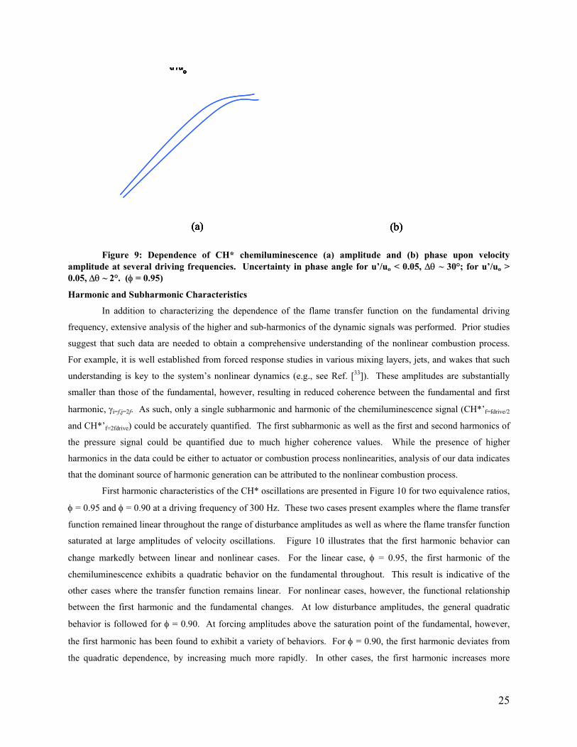
Figure 9: Dependence of CH* chemiluminescence (a) amplitude and (b) phase upon
velocity amplitude at several driving frequencies. Uncertainty in phase angle for u’/uo
< 0.05, ∆θ ~ 30°; for u’/uo > 0.05, ∆θ ~ 2°. (φ = 0.95)....................................................... 25
Figure 10: Dependence of CH* 1st harmonic on the square of CH* fundamental at two
equivalence ratios (fdrive = 300 Hz)..................................................................................... 26
Figure 11: Dependence of pressure harmonic amplitude on velocity oscillation amplitude
(fdrive = 290 Hz, φ = 0.95). Quadratic trend indicated by the solid line, cubic trend
indicated by dashed line. .................................................................................................... 26
5
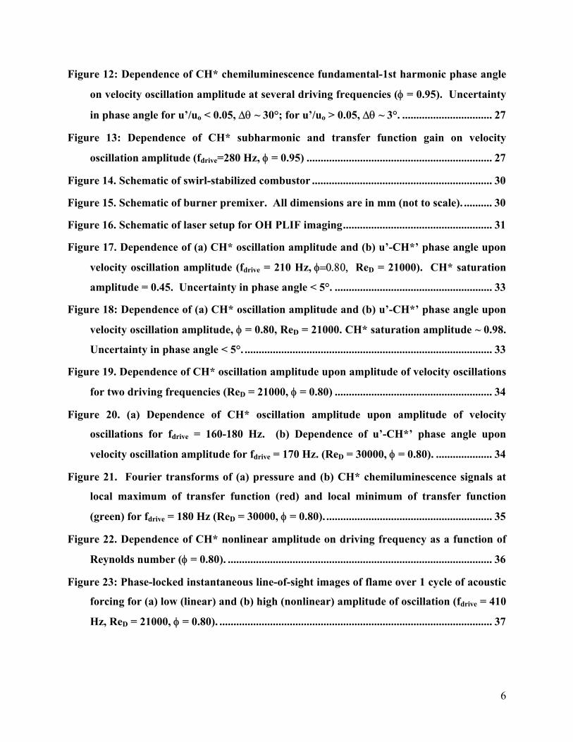
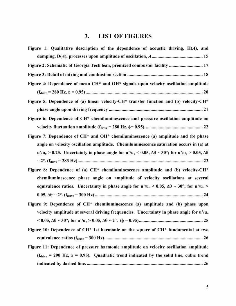
Figure 12: Dependence of CH* chemiluminescence fundamental-1st harmonic phase angle
on velocity oscillation amplitude at several driving frequencies (φ = 0.95). Uncertainty
in phase angle for u’/uo < 0.05, ∆θ ~ 30°; for u’/uo > 0.05, ∆θ ~ 3°. ................................ 27
Figure 13: Dependence of CH* subharmonic and transfer function gain on velocity
oscillation amplitude (fdrive=280 Hz, φ = 0.95) .................................................................. 27
Figure 14. Schematic of swirl-stabilized combustor ................................................................ 30
Figure 15. Schematic of burner premixer. All dimensions are in mm (not to scale). .......... 30
Figure 16. Schematic of laser setup for OH PLIF imaging..................................................... 31
Figure 17. Dependence of (a) CH* oscillation amplitude and (b) u’-CH*’ phase angle upon
velocity oscillation amplitude (fdrive = 210 Hz, φ=0.80, ReD = 21000). CH* saturation
amplitude = 0.45. Uncertainty in phase angle < 5°. ........................................................ 33
Figure 18: Dependence of (a) CH* oscillation amplitude and (b) u’-CH*’ phase angle upon
velocity oscillation amplitude, φ = 0.80, ReD = 21000. CH* saturation amplitude ~ 0.98.
Uncertainty in phase angle < 5°. ........................................................................................ 33
Figure 19. Dependence of CH* oscillation amplitude upon amplitude of velocity oscillations
for two driving frequencies (ReD = 21000, φ = 0.80) ........................................................ 34
Figure 20. (a) Dependence of CH* oscillation amplitude upon amplitude of velocity
oscillations for fdrive = 160-180 Hz. (b) Dependence of u’-CH*’ phase angle upon
velocity oscillation amplitude for fdrive = 170 Hz. (ReD = 30000, φ = 0.80). .................... 34
Figure 21. Fourier transforms of (a) pressure and (b) CH* chemiluminescence signals at
local maximum of transfer function (red) and local minimum of transfer function
(green) for fdrive = 180 Hz (ReD = 30000, φ = 0.80). ........................................................... 35
Figure 22. Dependence of CH* nonlinear amplitude on driving frequency as a function of
Reynolds number (φ = 0.80). .............................................................................................. 36
Figure 23: Phase-locked instantaneous line-of-sight images of flame over 1 cycle of acoustic
forcing for (a) low (linear) and (b) high (nonlinear) amplitude of oscillation (fdrive = 410
Hz, ReD = 21000, φ = 0.80). ................................................................................................. 37
6
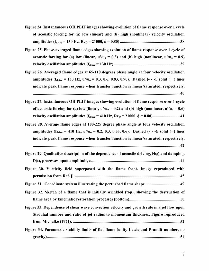
Figure 24. Instantaneous OH PLIF images showing evolution of flame response over 1 cycle
of acoustic forcing for (a) low (linear) and (b) high (nonlinear) velocity oscillation
amplitudes (fdrive = 130 Hz, ReD = 21000, φ = 0.80) .......................................................... 38
Figure 25. Phase-averaged flame edges showing evolution of flame response over 1 cycle of
acoustic forcing for (a) low (linear, u’/uo = 0.3) and (b) high (nonlinear, u’/uo = 0.9)
velocity oscillation amplitudes (fdrive = 130 Hz) ................................................................ 39
Figure 26. Averaged flame edges at 65-110 degrees phase angle at four velocity oscillation
amplitudes (fdrive = 130 Hz, u’/uo = 0.3, 0.6, 0.83, 0.90). Dashed (- - -)/ solid (___) lines
indicate peak flame response when transfer function is linear/saturated, respectively.
............................................................................................................................................... 40
Figure 27. Instantaneous OH PLIF images showing evolution of flame response over 1 cycle
of acoustic forcing for (a) low (linear, u’/uo = 0.2) and (b) high (nonlinear, u’/uo = 0.6)
velocity oscillation amplitudes (fdrive = 410 Hz, ReD = 21000, φ = 0.80).......................... 41
Figure 28. Average flame edges at 180-225 degree phase angle at four velocity oscillation
amplitudes (fdrive = 410 Hz, u’/uo = 0.2, 0.3, 0.53, 0.6). Dashed (- - -)/ solid (__) lines
indicate peak flame response when transfer function is linear/saturated, respectively.
............................................................................................................................................... 42
Figure 29. Qualitative description of the dependence of acoustic driving, H(ε) and damping,
D(ε), processes upon amplitude, ε ...................................................................................... 44
Figure 30. Vorticity field superposed with the flame front. Image reproduced with
permission from Ref. []....................................................................................................... 45
Figure 31. Coordinate system illustrating the perturbed flame shape ................................. 49
Figure 32. Sketch of a flame that is initially wrinkled (top), showing the destruction of
flame area by kinematic restoration processes (bottom)................................................. 50
Figure 33. Dependence of shear wave convection velocity and growth rate in a jet flow upon
Strouhal number and ratio of jet radius to momentum thickness. Figure reproduced
from Michalke (1971). ........................................................................................................ 52
Figure 34. Parametric stability limits of flat flame (unity Lewis and Prandlt number, no
gravity). ................................................................................................................................ 54
7
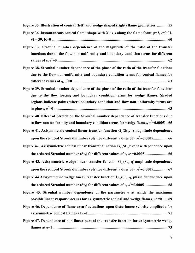
Figure 35. Illustration of conical (left) and wedge shaped (right) flame geometries. ........... 55
Figure 36. Instantaneous conical flame shape with X axis along the flame front. β=2, ε=0.01,
St = 39, K=0 ......................................................................................................................... 60
Figure 37. Strouhal number dependence of the magnitude of the ratio of the transfer
functions due to the flow non-uniformity and boundary condition terms for different
values of η, σ*=0 ................................................................................................................... 62
Figure 38. Strouhal number dependence of the phase of the ratio of the transfer functions
due to the flow non-uniformity and boundary condition terms for conical flames for
different values of η, σ*=0 ................................................................................................... 63
Figure 39. Strouhal number dependence of the phase of the ratio of the transfer functions
due to the flow forcing and boundary condition terms for wedge flames. Shaded
regions indicate points where boundary condition and flow non-uniformity terms are
in phase, σ*=0 ....................................................................................................................... 63
Figure 40. Effect of Stretch on the Strouhal number dependence of transfer functions due
to flow non-uniformity and boundary condition terms for wedge flames, σ*=0.0005 .. 65
Figure 41. Axisymmetric conical linear transfer function G (c 2St , )η magnitude dependence
upon the reduced Strouhal number (St2) for different values of η, σ*=0.0005............... 66
Figure 42. Axisymmetric conical linear transfer function G (c 2St , )η phase dependence upon
the reduced Strouhal number (St2) for different values of η, σ*=0.0005........................ 66
Figure 43. Axisymmetric wedge linear transfer function G (w 2St , )η amplitude dependence
upon the reduced Strouhal number (St2) for different values of η, σ*=0.0005............... 67
Figure 44 Axisymmetric wedge linear transfer function G (w 2St , )η phase dependence upon
the reduced Strouhal number (St2) for different values of η, σ*=0.0005 ........................ 68
Figure 45. Strouhal number dependence of the parameter η at which the maximum
possible linear response occurs for axisymmetric conical and wedge flames, σ*=0 ..... 69
Figure 46. Dependence of flame area fluctuations upon disturbance velocity amplitude for
axisymmetric conical flames at η=1................................................................................... 71
Figure 47. Dependence of non-linear part of the transfer function for axisymmetric wedge
flames at η=1 ........................................................................................................................ 73
8
Figure 48. Strouhal number dependence of the ratio of the magnitude of the flame area-
velocity transfer function to its linear value for the axisymmetric wedge flame, β=1,
σ*=0.005 ................................................................................................................................ 74
Figure 49. Strouhal number dependence of the phase of the flame area-velocity transfer
function for the axisymmetric conical flame, β=1, σ*=0.005............................................ 74
Figure 50. Strouhal number dependence of the ratio of the magnitude of the flame area-
velocity transfer function to its linear value for the axisymmetric wedge flame, β=1,
σ*=0.005 ................................................................................................................................ 75
Figure 51. Strouhal number dependence of the phase of the flame area-velocity transfer
function for the axisymmetric wedge flame, β=1 , σ*=0.005 ............................................ 75
Figure 52. Strouhal number dependence of the magnitude of the flame area-velocity
transfer function for the axisymmetric wedge flame, α=0.8,K=2.5, σ*=0.005............... 76
Figure 53. Experimentally measured gain for an inverted conical flame for a mean velocity
uo= 2.05 m/s, φ = 0.92. Data reproduced from Durox et al............................................... 77
Figure 54. Dependence of non-linear part of the transfer function on the phase speed of the
disturbances (K) for axisymmetric wedge flames, St=1, σ=0 .......................................... 78
Figure 55. Dependence of the magnitude of the flame area-velocity transfer function on η
for the axisymmetric conical flame for different Strouhal numbers, β=8, σ=0. Arrow
points towards increasing velocity amplitude ε. ............................................................... 78
Figure 56. Dependence of acoustic driving, H(ε) (where H(ε) is equated for this example to
Aw’/Aw,o) and damping, D(ε), processes upon velocity amplitude ε, for wedge flames at
St2=6.25 with K=2, α =0.8, σ*=0.005................................................................................... 79
Figure 57. Qualitative representation of regions where nonlinear flame transfer exceeds
(shaded) or is less than (white) linear transfer function, α=0.8,ε=0.1, σ=0..................... 79
Figure 58. Amplitude dependence of the magnitude of the flame area-velocity transfer
function for an axisymmetric wedge flame: Comparison between models with and
without Stretch effects. β=1, K=0 ..................................................................................... 80
Figure 59. Dependence of flame area fluctuations upon disturbance velocity amplitude for
axisymmetric conical flames at η=1................................................................................... 82
9
Figure 60. Contours of constant Lavg (average flame length) as a function of K and St2 for
different values of α. Arrows indicate regions of increasing flame length..................... 82
Figure 61: Frequency–response curves at several excitation amplitudes for a second order
oscillator with nonlinearities in (a) stiffness and (b) damping........................................ 83
Figure 62: Dependence of pressure amplitude upon frequency at (a) a single disturbance
amplitude, 2.8A and (b) several disturbance amplitudes, 1.8-3.0A (φ = 0.95)............... 84
Figure 63: Excitation–response curves for softening spring oscillator at several excitation
frequencies. .......................................................................................................................... 85
Figure 64: Dependence of pressure oscillation amplitude on excitation amplitude for
varying driving frequencies (φ = 0.95) .............................................................................. 85
Figure 65: Amplitude-frequency ranges over which the chemiluminescence-pressure-
velocity relationship exhibited single and multi-valued behavior .................................. 86
Figure 66: Dependence of pressure-CH* transfer function on driving frequency (excitation
amplitude = 2.4 amperes (a), excitation amplitude = 3.0 amperes (b), φ = 0.95)........... 87
Figure 67: (a) Spectrum of combustor pressure at two driving amplitudes showing decrease
in combustor instability mode as driving amplitude is increased (instability frequency
= 461 Hz, driving frequency = 200 Hz). (b) Dependence of instability amplitude on
driving velocity amplitude at 200 Hz driving frequency................................................. 88
Figure 68: Dependence of instability amplitude on driving amplitude for driving frequency
= 410 Hz (instability frequency = 461 Hz). ....................................................................... 90
Figure 69: Dependence of (a) velocity entrainment amplitude, AE, and (b) corresponding
pressure amplitude values upon driving frequency (instability frequency = 461 Hz).. 90
Figure 70: Dependence of instability rolloff, δp on driving frequency (instability frequency
= 461 Hz) .............................................................................................................................. 91
Figure 71: Dependence of AL parameter (velocity oscillation amplitude range which is
independent of forcing) on driving frequency (instability frequency = 461 Hz)........... 91
Figure 72: Dependence of maximum acoustic power reduction on driving frequency
(instability frequency = 461 Hz). ....................................................................................... 92
10
Figure 73. Block diagram of gain/phase shifter between pressure transducer and air
actuator used to generate self-excited oscillations. .......................................................... 94
Figure 74 Low pass filtered time dependence of oscillatory combustor pressure amplitude
with and without control. ................................................................................................... 96
Figure 75. Dependence of mean and fluctuating instability amplitude upon desired level. 96
Figure 76. Fourier transform of combustor pressure at desired amplitude levels of 0-0.4
psi.......................................................................................................................................... 97
Figure 77. Fourier transform of combustor pressure at desired amplitude levels of 0.4, 0.2,
0.16, 0.14, and 0.13 psi (nominal instability amplitude = 0.35 psi). ................................ 98
Figure 78 Instability driving characteristic visualized by plotting the dependence of the
instantaneous air actuator driving signal upon pressure................................................ 99
Figure 79. Dependence of instantaneous pressure amplitude upon time as phase of control
signal is swept relative to that of the instability. .............................................................. 99
11
4. EXECUTIVE SUMMARY
Under the High Efficiency Engines and Turbines-University Turbine Research (HEET-UTSR) program,
Georgia Institute of Technology is investigating the mechanisms and control of detrimental oscillations in gas
turbine combustors. This program consists of two main tasks. The first task is investigating the dynamics of
uncontrolled combustors. These results are improving capabilities to predict the occurrence and amplitudes of
instabilities. The second task is investigating active control of combustion dynamics. This work is developing
methods for suppressing these instabilities in the highly turbulent, harsh combustor environment and improving
understanding of the factors that effect active control authority. Currently, combustion dynamics severely reduce
the reliability and availability of gas turbines by damaging parts and substantially reducing time between overhauls,
both of which ultimately affect the consumer by increasing the cost of electricity.
This program investigates the causes and active control of combustion driven oscillations in low emissions
gas turbines. These oscillations are a critical problem encountered in the development of new systems and the
availability and maintainability of fielded systems. This document is the final report under this contract . During
the duration of the contract, substantial progress has been made in improving the understanding of the dynamics of
unstable combustors. Both experimental and theoretical efforts have been pursued and completed over the period of
the contract.
This report describes all of the experimental and theoretical work undertaken during the last 3-1/2 years.
Specifically, this report describes experimental studies which investigated the mechanisms responsible for saturation
of the flame transfer function and therefore control the limit cycle amplitude of unstable gas turbine combustors. In
addition, theoretical studies utilizing one possible mechanism were performed to investigate nonlinear flame
response behavior.
Furthermore, experiments on unstable combustors including active control studies and nonlinear frequency
interaction investigations were performed to improve the understanding of the underlying physics which control
combustion instabilities.
Interactions with industrial partners was also a priority during this contract. We have initiated a program
with an OEM to incorporate and validate the modeling work performed under this program into their in-house
prediction codes. We also maintain regular discussions with combustion engineers at many of the OEM’s.
12
5. PROJECT DESCRIPTION
Under the High Efficiency Engines and Turbines-University Turbine Research (HEET-UTSR) program,
Georgia Institute of Technology is investigating the mechanisms and control of detrimental oscillations in gas
turbine combustors. This program consists of two main tasks. The first task is investigating the dynamics of
uncontrolled combustors. These results are improving capabilities to predict the occurrence and amplitudes of
instabilities. The second task is investigating active control of combustion dynamics. This work is developing
methods for suppressing these instabilities in the highly turbulent, harsh combustor environment and improving
understanding of the factors that effect active control authority.
Currently, combustion dynamics severely reduces the reliability and availability of gas turbines by
damaging parts and substantially reducing time between overhauls, both of which ultimately affect the consumer by
increasing the cost of electricity. This work will result in improved understanding of the processes that cause these
oscillations and strategies to eliminate them. Successful completion of this project will benefit the gas turbine and
energy industry in several ways. First, through its improvement of turbine reliability and availability, it will reduce
maintenance needs and costly downtime. In addition, it will broaden the operating envelope of gas turbines, so that
they will be able to operate at higher power as well as at idle without worry of damaging oscillations. For example,
many fielded turbines are not able to operate at full power because of the enormous dynamics problems encountered
there. Elimination of the dynamics problem will allow them to increase their maximum power, thereby improving
their capabilities to respond to peak power demands.
13
6. NONLINEAR FLAME TRANSFER FUNCTION
CHARACTERISTICS
This section describes an experimental investigation of the relationship between flow disturbances and heat
release oscillations in a lean, premixed combustor. This work is motivated by the fact that combustion instabilities
continue to be one of the most serious issues hindering the development and operation of industrial gas turbines1-4.
These instabilities generally occur when the unsteady combustion process couples with one or more of the natural
acoustic modes of the combustion chamber, resulting in self-excited oscillations. These oscillations adversely affect
engine performance and emissions, and can be destructive to engine hardware.
Our focus here is on the amplitude response of the heat release at some frequency, f, to a harmonic
disturbance of amplitude, A, at that same frequency. The heat release response, H(A), generally exhibits a linear
dependence upon the disturbance amplitude at small values of A. At high amplitudes, however, they are related
nonlinearly. This is significant because the dynamics of an unstable combustor are controlled by both linear and
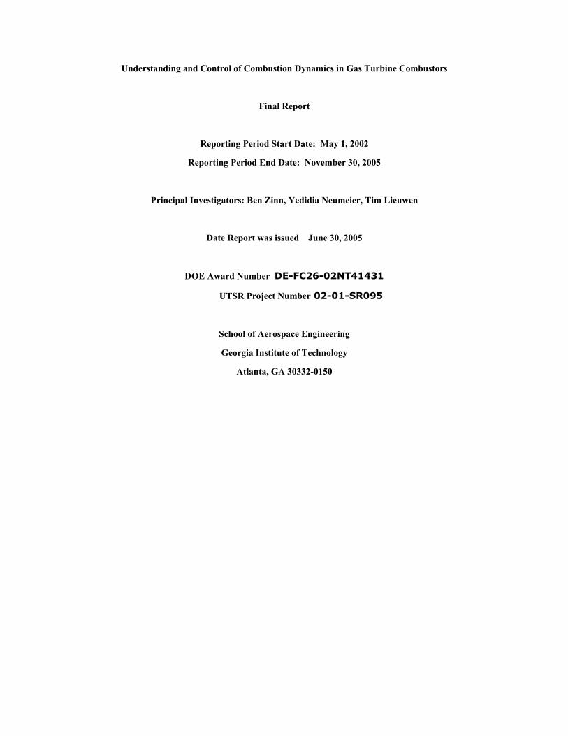
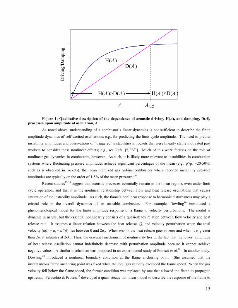
nonlinear processes. This can be seen from Figure 1, which plots the amplitude dependence of hypothetical driving,
H(A), and damping, D(A), processes. Note that the disturbance amplitude stays the same, decreases, or increases
depending upon whether H(A)=D(A), H(A)<D(A), or H(A)>D(A), respectively. Linear combustor processes
generally control the balance between driving and damping processes at low amplitudes of oscillation, H(A)-D(A),
and, thus, determine the frequency and growth rate, A~eαt, of inherent disturbances in the combustor. Note that the
initial growth rate of the instability, α, is proportional to the difference between the driving and damping processes
in the linear regime. Nonlinear combustor processes control the finite amplitude dynamics of the oscillations. For
example, predicting the limit cycle amplitude of self-excited oscillations requires an understanding of the nonlinear
characteristics of H(A) and D(A). To illustrate, Figure 1 depicts a situation where H(A) saturates and D(A) remains
linear, so that the two curves cross at the limit cycle amplitude, ALC.
Understanding of a combustor’s linear dynamics is needed to predict the frequency and conditions under
which inherent disturbances in the combustor grow or decay. As a result of extensive work in this area, capabilities
for modeling the acoustics of the combustor system are reasonably well developed (e.g., see Refs. [5,6]). Also,
capabilities for modeling the interactions of flow and mixture disturbances with flames, needed to predict the
conditions under which instabilities occur, are improving rapidly7,8. Much of this work is being transitioned to
industry and being incorporated into dynamics predictions codes. In fact, most gas turbine manufacturers have
reported model development efforts for predicting instability frequencies, mode shapes, and conditions of
occurrence9-11.
14
A
Driv
ing/
Dam
ping
D(A )
H(A )
A LC
H(A )>D(A ) H(A )<D(A )
Figure 1: Qualitative description of the dependence of acoustic driving, H(A), and damping, D(A), processes upon amplitude of oscillation, A
As noted above, understanding of a combustor’s linear dynamics is not sufficient to describe the finite
amplitude dynamics of self-excited oscillations; e.g., for predicting the limit cycle amplitude. The need to predict
instability amplitudes and observations of “triggered” instabilities in rockets that were linearly stable motivated past
workers to consider these nonlinear effects; e.g., see Refs. [5, 12-14]. Much of this work focuses on the role of
nonlinear gas dynamics in combustors, however. As such, it is likely more relevant to instabilities in combustion
systems where fluctuating pressure amplitudes achieve significant percentages of the mean (e.g., p’/po ~20-50%,
such as is observed in rockets), than lean premixed gas turbine combustors where reported instability pressure
amplitudes are typically on the order of 1-5% of the mean pressure2, 15.
Recent studies15-18 suggest that acoustic processes essentially remain in the linear regime, even under limit
cycle operation, and that it is the nonlinear relationship between flow and heat release oscillations that causes
saturation of the instability amplitude. As such, the flame’s nonlinear response to harmonic disturbances may play a
critical role in the overall dynamics of an unstable combustor. For example, Dowling16 introduced a
phenomenological model for the finite amplitude response of a flame to velocity perturbations. The model is
dynamic in nature, but the essential nonlinearity consists of a quasi-steady relation between flow velocity and heat
release rate. It assumes a linear relation between the heat release, Q, and velocity perturbation when the total
velocity (u(t) = uo + u’(t)) lies between 0 and 2uo. When u(t)<0, the heat release goes to zero and when it is greater
than 2uo it saturates at 2Qo. Thus, the essential mechanism of nonlinearity lies in the fact that the lowest amplitude
of heat release oscillation cannot indefinitely decrease with perturbation amplitude because it cannot achieve
negative values. A similar mechanism was proposed in an experimental study of Poinsot et al.19. In another study,
Dowling 20 introduced a nonlinear boundary condition at the flame anchoring point. She assumed that the
instantaneous flame anchoring point was fixed when the total gas velocity exceeded the flame speed. When the gas
velocity fell below the flame speed, the former condition was replaced by one that allowed the flame to propagate
upstream. Peracchio & Proscia17 developed a quasi-steady nonlinear model to describe the response of the flame to
15
equivalence ratio perturbations. They assumed the following relationship for the response of the instantaneous
mixture composition leaving the nozzle exit to velocity perturbations:
( ) u/tuk1)t(
′+=
φφ (1)
where k is a constant with a value near unity. They also utilized a nonlinear relationship relating the heat release per
unit mass of mixture to the instantaneous equivalence ratio. Wu et al.18 developed a more general asymptotic
analysis which focuses on the nonlinear interaction/coupling among acoustic, vortical, and Darrieus-Landau
instability modes at the flame. This theory is found to agree well with the experimental work presented in Searby21.
Several of the above analyses suggest that the ratio of fluctuating and mean velocity, u’/uo, is an important
non-dimensional parameter that controls the amplitude of the limit cycle oscillations through its effect upon the
nonlinear relationship between flow disturbances and heat release oscillations. A similar conclusion was reached
empirically in an experimental study of Lieuwen15, who found that combustion instability amplitudes had a strong
dependence upon a mean combustor velocity scale, uo.
In an effort to understand the mechanisms controlling the growth rates and limit cycle amplitudes of
combustion instabilities, the response of the flame under external forcing of the flow field has been analyzed by
several researchers (e.g., see Refs.[22-26]). Külsheimer & Büchner22 measured the effect of driving frequency and
amplitude on premixed swirled and unswirled flames. They characterized the conditions under which large-scale
coherent ring-vortex structure were evident, a key mechanism for self-excited oscillations, as well as the resulting
flame response, on driving amplitude and frequency. They found that vortex formation occurred at lower driving
amplitudes as the driving frequency was increased. Furthermore, the peak flame response in swirl flames shifted to
higher frequencies for larger flow perturbations. No explicit characterization of the nonlinear interaction between
the flame’s heat release and the flow perturbations were reported, however.
The potentially significant nonlinear relationship between acoustic perturbations and heat release
perturbations suggested by the theoretical studies above, are also supported by recent measurements of Lieuwen &
Neumeier23, Lee & Santavicca24, and Balachandran et al.26 who characterized the pressure-heat release relationship
as a function of oscillation amplitude. The former study found that this relationship was linear for pressure
amplitudes below about 1% of the mean pressure. At higher forcing levels, they found that the heat release
oscillation amplitude began to saturate. In contrast to the assumed model of Dowling16, however, Lieuwen &
Neumeier found saturation to occur at CH*’/CH*o values of ~25%, in contrast to the 100% value assumed in her
model. Data were only obtained at one operating condition and two driving frequencies, however, so the manner in
which these saturation characteristics depend upon operating conditions and frequency is unclear.
Durox et al.27 and Bourehla & Baillot25 appear to have performed the only systematic study characterizing
the response of a non-swirling flame to large amplitude perturbations. Their study was performed on a laminar
Bunsen flame and primarily focused on its qualitative characteristics. No measurements of the dependence of
unsteady heat release or chemiluminescence emissions were reported. They found that at low frequencies (f < 200
Hz) and velocity amplitudes (u’/uo<0.3), the flame front wrinkles symmetrically about the burner axis due to a
16
convected wave traveling from the burner base to its tip. With increasing amplitude of low frequency velocity
perturbations, they found that the flame exhibited a variety of transient flame holding behavior, such as flashback,
asymmetric blowoff, and unsteady lifting and re-anchoring of the flame. In addition, they noted that its response
was asymmetric and disordered. Finally, at high frequencies and forcing amplitudes (u’/uo>1), they found that the
flame tip collapses to a hemispherical shape.
As can be seen from the above review, there is a need for systematic measurements of the flame’s nonlinear
response to flow perturbations, i.e. saturation of the curve H(A) in Figure 1. Such characteristics must be understood
in order to, for example, predict instability amplitudes or model the transient response of a combustor to active
control. As such, we obtained measurements of the pressure/ velocity/ chemiluminescence amplitude and phase
relationships in a swirling flame over a range of driving amplitudes. These results were obtained by externally
driving oscillations in the combustor with varying amplitudes. Measurements were obtained at several driving
frequencies and fuel/air ratio.
Gas Turbine Combustor Simulator
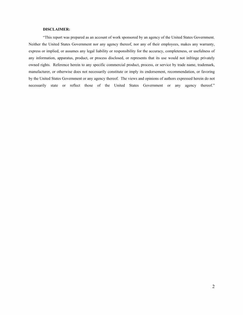
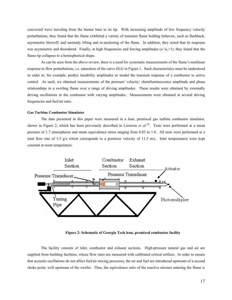
The data presented in this paper were measured in a lean, premixed gas turbine combustor simulator,
shown in Figure 2, which has been previously described in Lieuwen et al.28. Tests were performed at a mean
pressure of 1.7 atmospheres and mean equivalence ratios ranging from 0.83 to 1.0. All tests were performed at a
total flow rate of 5.5 g/s which corresponds to a premixer velocity of 11.5 m/s. Inlet temperatures were kept
constant at room temperature.
Figure 2: Schematic of Georgia Tech lean, premixed combustor facility
The facility consists of inlet, combustor and exhaust sections. High-pressure natural gas and air are
supplied from building facilities, whose flow rates are measured with calibrated critical orifices. In order to ensure
that acoustic oscillations do not affect fuel/air mixing processes, the air and fuel are introduced upstream of a second
choke point, well upstream of the swirler. Thus, the equivalence ratio of the reactive mixture entering the flame is
17
essentially constant. This was done because of the sensitivity of the flame chemiluminescence levels to both heat
release rate and equivalence ratio. If the equivalence ratio and heat release rate simultaneously vary, monitoring the
flame chemiluminescence alone would not be sufficient to infer information about heat release fluctuations24. Note
that the fuel/air mixing processes were not acoustically isolated in the previous study of Lieuwen & Neumeier23.
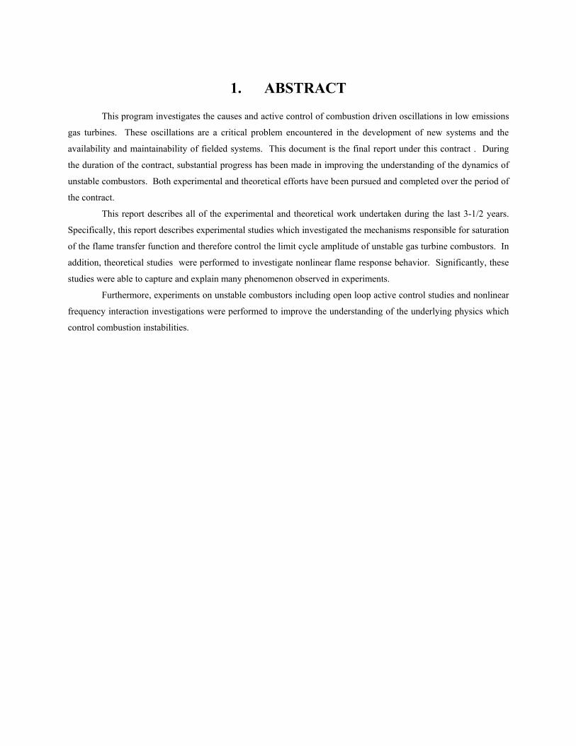
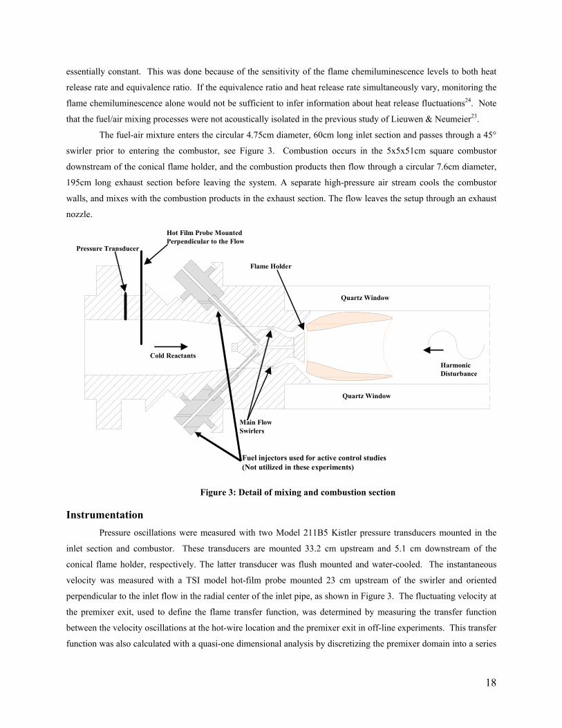
The fuel-air mixture enters the circular 4.75cm diameter, 60cm long inlet section and passes through a 45°
swirler prior to entering the combustor, see Figure 3. Combustion occurs in the 5x5x51cm square combustor
downstream of the conical flame holder, and the combustion products then flow through a circular 7.6cm diameter,
195cm long exhaust section before leaving the system. A separate high-pressure air stream cools the combustor
walls, and mixes with the combustion products in the exhaust section. The flow leaves the setup through an exhaust
nozzle.
Cold Reactants
Hot Film Probe Mounted Perpendicular to the Flow
Pressure Transducer
Main Flow Swirlers
Quartz Window
Quartz Window
Harmonic Disturbance
Flame Holder
Cold Reactants
Hot Film Probe Mounted Perpendicular to the Flow
Pressure Transducer
Main Flow Swirlers
Quartz Window
Quartz Window
Harmonic Disturbance
Flame Holder
Fuel injectors used for active control studies (Not utilized in these experiments)
Cold Reactants
Hot Film Probe Mounted Perpendicular to the Flow
Pressure Transducer
Main Flow Swirlers
Quartz Window
Quartz Window
Harmonic Disturbance
Flame Holder
Cold Reactants
Hot Film Probe Mounted Perpendicular to the Flow
Pressure Transducer
Main Flow Swirlers
Quartz Window
Quartz Window
Harmonic Disturbance
Flame Holder
Fuel injectors used for active control studies (Not utilized in these experiments)
Figure 3: Detail of mixing and combustion section
Instrumentation Pressure oscillations were measured with two Model 211B5 Kistler pressure transducers mounted in the
inlet section and combustor. These transducers are mounted 33.2 cm upstream and 5.1 cm downstream of the
conical flame holder, respectively. The latter transducer was flush mounted and water-cooled. The instantaneous
velocity was measured with a TSI model hot-film probe mounted 23 cm upstream of the swirler and oriented
perpendicular to the inlet flow in the radial center of the inlet pipe, as shown in Figure 3. The fluctuating velocity at
the premixer exit, used to define the flame transfer function, was determined by measuring the transfer function
between the velocity oscillations at the hot-wire location and the premixer exit in off-line experiments. This transfer
function was also calculated with a quasi-one dimensional analysis by discretizing the premixer domain into a series
18
of regions characterized by their lengths and cross-sectional areas, and applying momentum and energy conservation
at the interfaces (see Ref. [6]). The swirler was modeled as a resistance that was determined from the flow velocity
and measured mean pressure drop. The model and measurements agreed very well over the 10-550 Hz frequency
range, except in transfer function magnitude in the vicinity of 80 and 420 Hz. At these frequencies, the transfer
function has large values (on the order of 5) and the model and measurements disagree by 100% in the peak
magnitude; however, they agree quite well in predicting the frequencies at which these occur. At all other
frequencies, the transfer function magnitude is essentially constant and equal to the cross sectional area ratio
between the two points, as expected from quasi-steady considerations. Because of the sensitive frequency
dependence of the velocity transfer function between the measurement location and premixer exit plane at 80 and
420 Hz, no nonlinear forced response studies were performed at these frequencies.
Global CH* and OH* chemiluminescence measurements were obtained with a photomultiplier tube (PMT)
fitted with 10 nm bandwidth filters centered at 430 and 310 nm, respectively. The PMT was installed downstream
of a quartz window at the rear end of the setup, see Figure 2. This arrangement permitted it to view the entire
combustion zone. The linearity of the PMT output was verified over the entire range of instantaneous light intensity
levels seen in these experiments. Data were obtained with a National Instruments DAQ controlled by Labview
software at a sampling rate of 10 kHz. A total of 16,384 data points were taken during each test.
Oscillations were driven in the combustor with an actuator developed at Georgia Tech for active
combustion control applications29. The actuator was mounted 5m downstream of the flame zone. It is capable of
driving oscillations over a frequency range of approximately 0-1500Hz. The actuator modulates a constant
secondary supply of air that is introduced near the combustor exit by periodically varying the degree of constriction
of a valve. Maximum amplitude of driving occurs when the flow passage is completely blocked for a portion of the
cycle and, thus, the actuator modulates 100% of the flow through the valve. The amplitude of forcing can be
controlled via the supply pressure of air to the actuator.
Forced Flame Characteristics
The basic experimental procedure consists of externally driving oscillations in the combustor with varying
amplitude at a fixed frequency or fixed amplitude at varying frequencies while obtaining simultaneous
measurements of pressure, velocity, and chemiluminescence. For all cases, the combustor was quite stable in the
absence of driving. The flame length ranged from 5-15cm between the equivalence ratios of 1.0-0.83, respectively.
Driving Effects on Average Flame and Coherence Characteristics
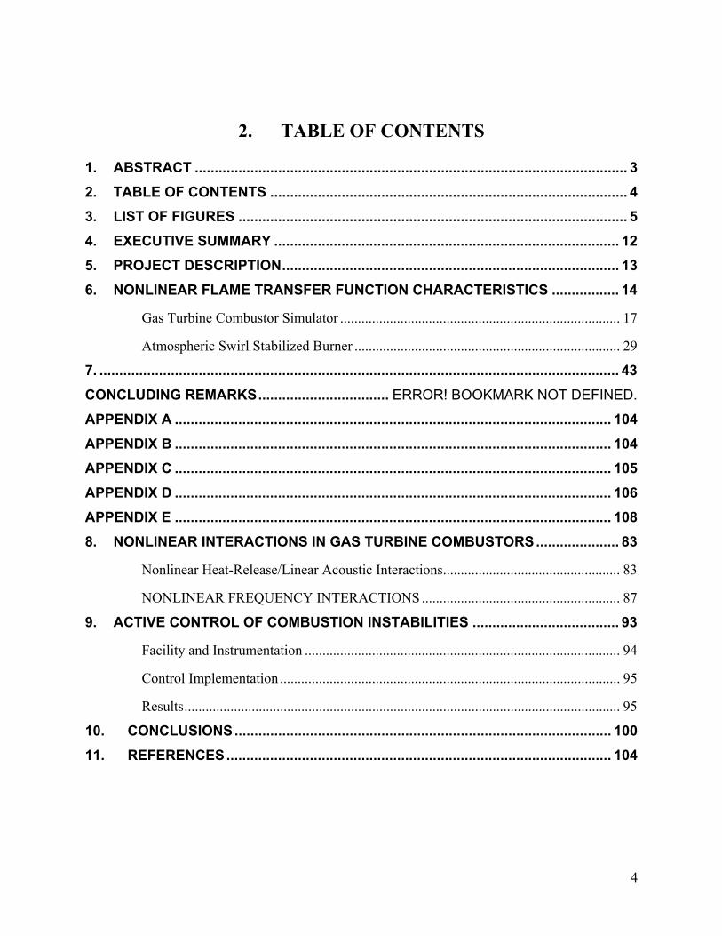
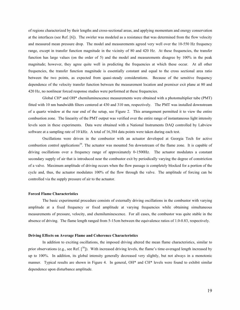
In addition to exciting oscillations, the imposed driving altered the mean flame characteristics, similar to
prior observations (e.g., see Ref. [30]). With increased driving levels, the flame’s time-averaged length increased by
up to 100%. In addition, its global intensity generally decreased very slightly, but not always in a monotonic
manner. Typical results are shown in Figure 4. In general, OH* and CH* levels were found to exhibit similar
dependence upon disturbance amplitude.
19
0 0.05 0.1 0.15 0.2 0.25 0.3 0.350
0.5
1
1.5
2
2.5
u′/uo
CH* o (a.u.)
0 0.05 0.1 0.15 0.2 0.25 0.3 0.350
0.2
0.4
0.6
0.8
1
OH*o (a.u.)
Figure 4: Dependence of mean CH* and OH* signals upon velocity oscillation amplitude (fdrive = 280
Hz, φ = 0.95)
In order to obtain accurate transfer function data, it is important to have good coherence between the
pressure, velocity and chemiluminescence oscillations at the frequency of interest. This was always achieved except
at the lowest driving amplitudes; typical coherence values were greater than 0.95. The effect of nonlinearities is to
also decrease the coherence value, so we would not expect perfect coherence values, even if the input-output
variables were perfectly correlated.
The amplitudes of the oscillations were determined by integrating the area under the power spectrum in the
vicinity of the driving frequency. The RMS levels of the oscillations were determined from these values via
Parseval’s relation and then multiplied by 2 to obtain the fluctuating amplitude. This procedure is equivalent to
determining the fluctuating amplitude after bandpass filtering the signal about the driving frequency. The phases of
the fluctuating parameters were determined from their Fourier transforms at the driving frequency.
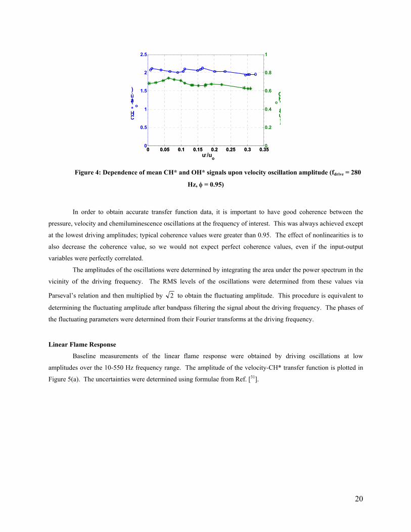
Linear Flame Response
Baseline measurements of the linear flame response were obtained by driving oscillations at low
amplitudes over the 10-550 Hz frequency range. The amplitude of the velocity-CH* transfer function is plotted in
Figure 5(a). The uncertainties were determined using formulae from Ref. [31].
20
00 400 500 600ncy (Hz)
0 100 200 300 400 500 6000
100
200
300
400
500
600
700
800
900
Frequency (Hz)
θ uE (d
egre
es)
00 400 500 600ncy (Hz)00 400 500 600ncy (Hz)
0 100 200 300 400 500 6000
100
200
300
400
500
600
700
800
900
Frequency (Hz)
θ uE (d
egre
es)
0 100 200 300 400 500 6000
100
200
300
400
500
600
700
800
900
Frequency (Hz)
θ uE (d
egre
es)
(a) (b)
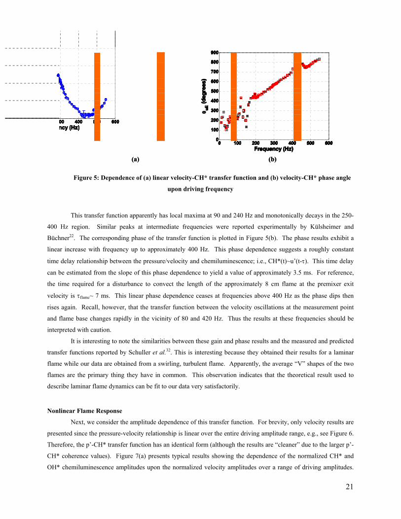
Figure 5: Dependence of (a) linear velocity-CH* transfer function and (b) velocity-CH* phase angle
upon driving frequency
This transfer function apparently has local maxima at 90 and 240 Hz and monotonically decays in the 250-
400 Hz region. Similar peaks at intermediate frequencies were reported experimentally by Külsheimer and
Büchner22. The corresponding phase of the transfer function is plotted in Figure 5(b). The phase results exhibit a
linear increase with frequency up to approximately 400 Hz. This phase dependence suggests a roughly constant
time delay relationship between the pressure/velocity and chemiluminescence; i.e., CH*(t)~u’(t-τ). This time delay
can be estimated from the slope of this phase dependence to yield a value of approximately 3.5 ms. For reference,
the time required for a disturbance to convect the length of the approximately 8 cm flame at the premixer exit
velocity is τflame~ 7 ms. This linear phase dependence ceases at frequencies above 400 Hz as the phase dips then
rises again. Recall, however, that the transfer function between the velocity oscillations at the measurement point
and flame base changes rapidly in the vicinity of 80 and 420 Hz. Thus the results at these frequencies should be
interpreted with caution.
It is interesting to note the similarities between these gain and phase results and the measured and predicted
transfer functions reported by Schuller et al.32. This is interesting because they obtained their results for a laminar
flame while our data are obtained from a swirling, turbulent flame. Apparently, the average “V” shapes of the two
flames are the primary thing they have in common. This observation indicates that the theoretical result used to
describe laminar flame dynamics can be fit to our data very satisfactorily.
Nonlinear Flame Response
Next, we consider the amplitude dependence of this transfer function. For brevity, only velocity results are
presented since the pressure-velocity relationship is linear over the entire driving amplitude range, e.g., see Figure 6.
Therefore, the p’-CH* transfer function has an identical form (although the results are “cleaner” due to the larger p’-
CH* coherence values). Figure 7(a) presents typical results showing the dependence of the normalized CH* and
OH* chemiluminescence amplitudes upon the normalized velocity amplitudes over a range of driving amplitudes.
21
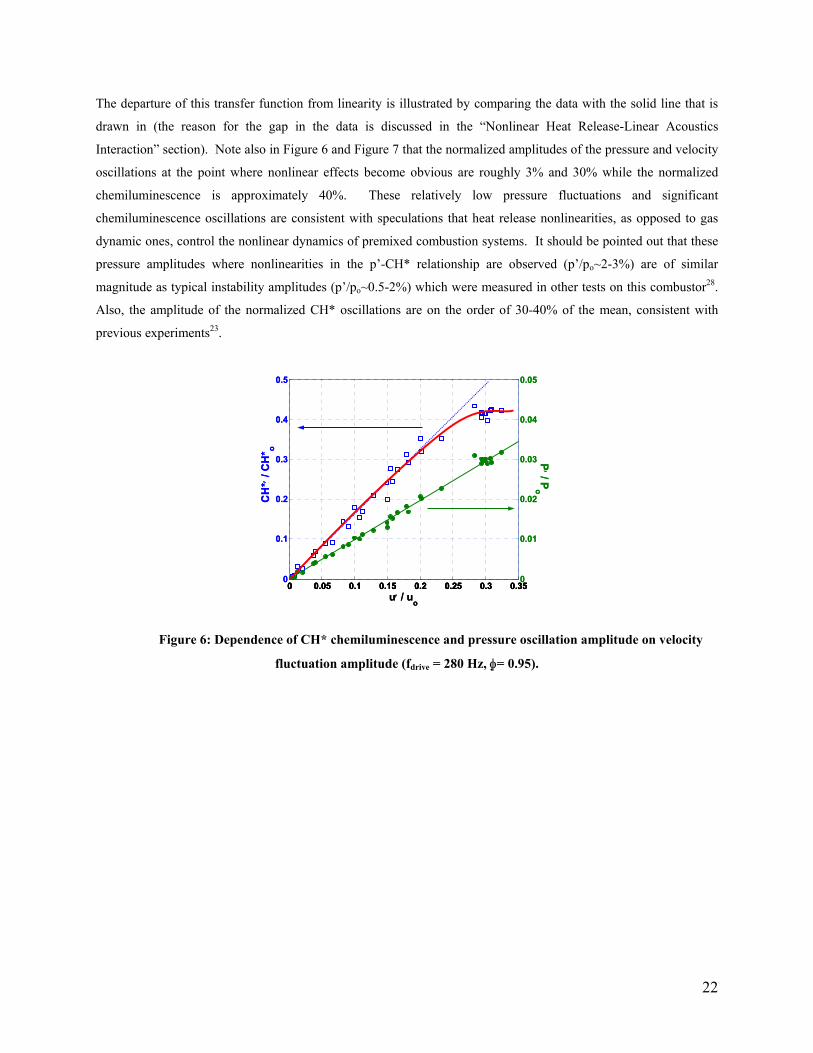
The departure of this transfer function from linearity is illustrated by comparing the data with the solid line that is
drawn in (the reason for the gap in the data is discussed in the “Nonlinear Heat Release-Linear Acoustics
Interaction” section). Note also in Figure 6 and Figure 7 that the normalized amplitudes of the pressure and velocity
oscillations at the point where nonlinear effects become obvious are roughly 3% and 30% while the normalized
chemiluminescence is approximately 40%. These relatively low pressure fluctuations and significant
chemiluminescence oscillations are consistent with speculations that heat release nonlinearities, as opposed to gas
dynamic ones, control the nonlinear dynamics of premixed combustion systems. It should be pointed out that these
pressure amplitudes where nonlinearities in the p’-CH* relationship are observed (p’/po~2-3%) are of similar
magnitude as typical instability amplitudes (p’/po~0.5-2%) which were measured in other tests on this combustor28.
Also, the amplitude of the normalized CH* oscillations are on the order of 30-40% of the mean, consistent with
previous experiments23.
0 0.05 0.1 0.15 0.2 0.25 0.3 0.350
0.1
0.2
0.3
0.4
0.5
u′ / uo
CH
* ′ / C
H* o
0 0.05 0.1 0.15 0.2 0.25 0.3 0.350
0.01
0.02
0.03
0.04
0.05
P′ / P
o
0 0.05 0.1 0.15 0.2 0.25 0.3 0.350
0.1
0.2
0.3
0.4
0.5
u′ / uo
CH
* ′ / C
H* o
0 0.05 0.1 0.15 0.2 0.25 0.3 0.350
0.01
0.02
0.03
0.04
0.05
P′ / P
o
Figure 6: Dependence of CH* chemiluminescence and pressure oscillation amplitude on velocity
fluctuation amplitude (fdrive = 280 Hz, φ= 0.95).
22
0 0.05 0.1 0.15 0.2 0.25 0.3 0.350
0.1
0.2
0.3
0.4
0.5
u′/uo
Nor
mal
ized
Che
milu
min
esce
nce
OH*′/OH*oCH*′/CH*o
0 0.05 0.1 0.15 0.2 0.25 0.3 0.35-40
-20
0
20
40
60
u′/uo
θuE
(degrees)
CH*′/CH*oOH*′/OH*o
(a) (b)
0 0.05 0.1 0.15 0.2 0.25 0.3 0.350
0.1
0.2
0.3
0.4
0.5
u′/uo
Nor
mal
ized
Che
milu
min
esce
nce
OH*′/OH*oCH*′/CH*o
0 0.05 0.1 0.15 0.2 0.25 0.3 0.35-40
-20
0
20
40
60
u′/uo
θuE
(degrees)
CH*′/CH*oOH*′/OH*o
(a) (b)
SaturationSaturationSaturation
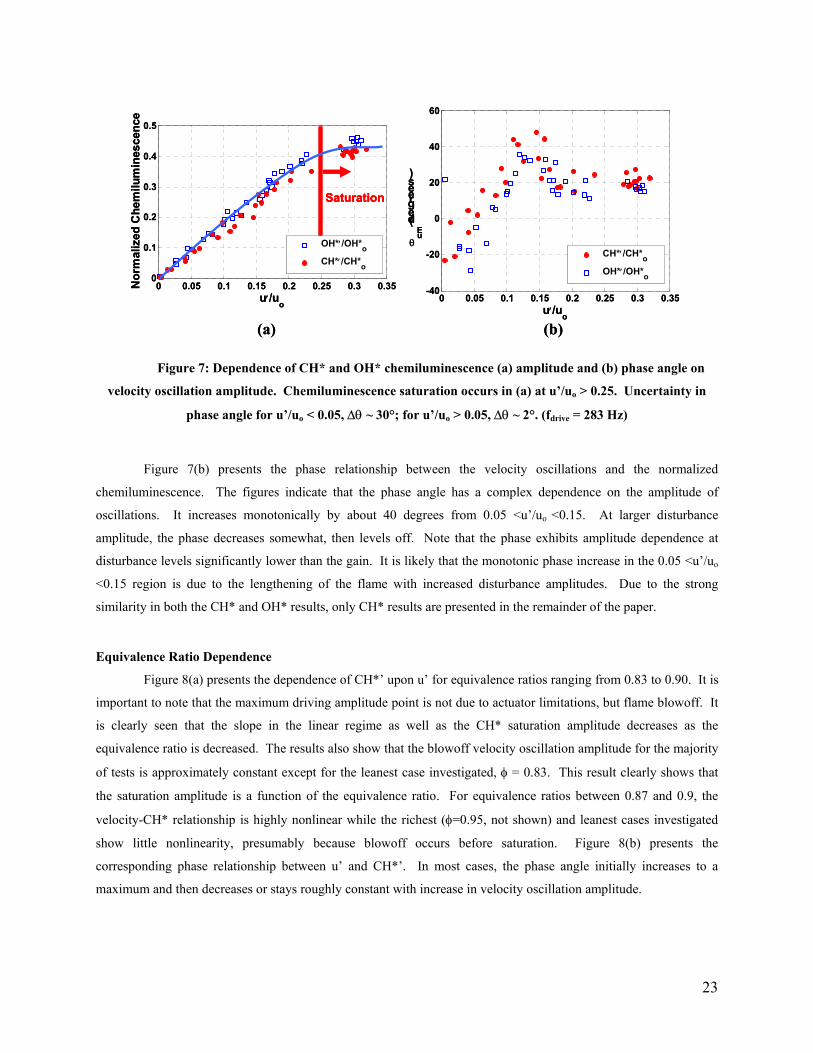
Figure 7: Dependence of CH* and OH* chemiluminescence (a) amplitude and (b) phase angle on
velocity oscillation amplitude. Chemiluminescence saturation occurs in (a) at u’/uo > 0.25. Uncertainty in
phase angle for u’/uo < 0.05, ∆θ ~ 30°; for u’/uo > 0.05, ∆θ ~ 2°. (fdrive = 283 Hz)
Figure 7(b) presents the phase relationship between the velocity oscillations and the normalized
chemiluminescence. The figures indicate that the phase angle has a complex dependence on the amplitude of
oscillations. It increases monotonically by about 40 degrees from 0.05 <u’/uo <0.15. At larger disturbance
amplitude, the phase decreases somewhat, then levels off. Note that the phase exhibits amplitude dependence at
disturbance levels significantly lower than the gain. It is likely that the monotonic phase increase in the 0.05 <u’/uo
<0.15 region is due to the lengthening of the flame with increased disturbance amplitudes. Due to the strong
similarity in both the CH* and OH* results, only CH* results are presented in the remainder of the paper.
Equivalence Ratio Dependence
Figure 8(a) presents the dependence of CH*’ upon u’ for equivalence ratios ranging from 0.83 to 0.90. It is
important to note that the maximum driving amplitude point is not due to actuator limitations, but flame blowoff. It
is clearly seen that the slope in the linear regime as well as the CH* saturation amplitude decreases as the
equivalence ratio is decreased. The results also show that the blowoff velocity oscillation amplitude for the majority
of tests is approximately constant except for the leanest case investigated, φ = 0.83. This result clearly shows that
the saturation amplitude is a function of the equivalence ratio. For equivalence ratios between 0.87 and 0.9, the
velocity-CH* relationship is highly nonlinear while the richest (φ=0.95, not shown) and leanest cases investigated
show little nonlinearity, presumably because blowoff occurs before saturation. Figure 8(b) presents the
corresponding phase relationship between u’ and CH*’. In most cases, the phase angle initially increases to a
maximum and then decreases or stays roughly constant with increase in velocity oscillation amplitude.
23
0 0.05 0.1 0.15 0.2 0.25 0.3-50
0
50
100
150
200
250
300
u′/uo
θ uE (d
egre
es)
φ=0.90φ=0.87φ=0.83
(a) (b)
0 0.05 0.1 0.15 0.2 0.25 0.30
0.05
0.1
0.15
0.2
0.25
0.3
0.35
u′/uo
CH
* ′/C
H* o
φ=0.90φ=0.87φ=0.83
0 0.05 0.1 0.15 0.2 0.25 0.3-50
0
50
100
150
200
250
300
u′/uo
θ uE (d
egre
es)
φ=0.90φ=0.87φ=0.83
(a) (b)
0 0.05 0.1 0.15 0.2 0.25 0.30
0.05
0.1
0.15
0.2
0.25
0.3
0.35
u′/uo
CH
* ′/C
H* o
φ=0.90φ=0.87φ=0.83
0 0.05 0.1 0.15 0.2 0.25 0.30
0.05
0.1
0.15
0.2
0.25
0.3
0.35
u′/uo
CH
* ′/C
H* o
φ=0.90φ=0.87φ=0.83
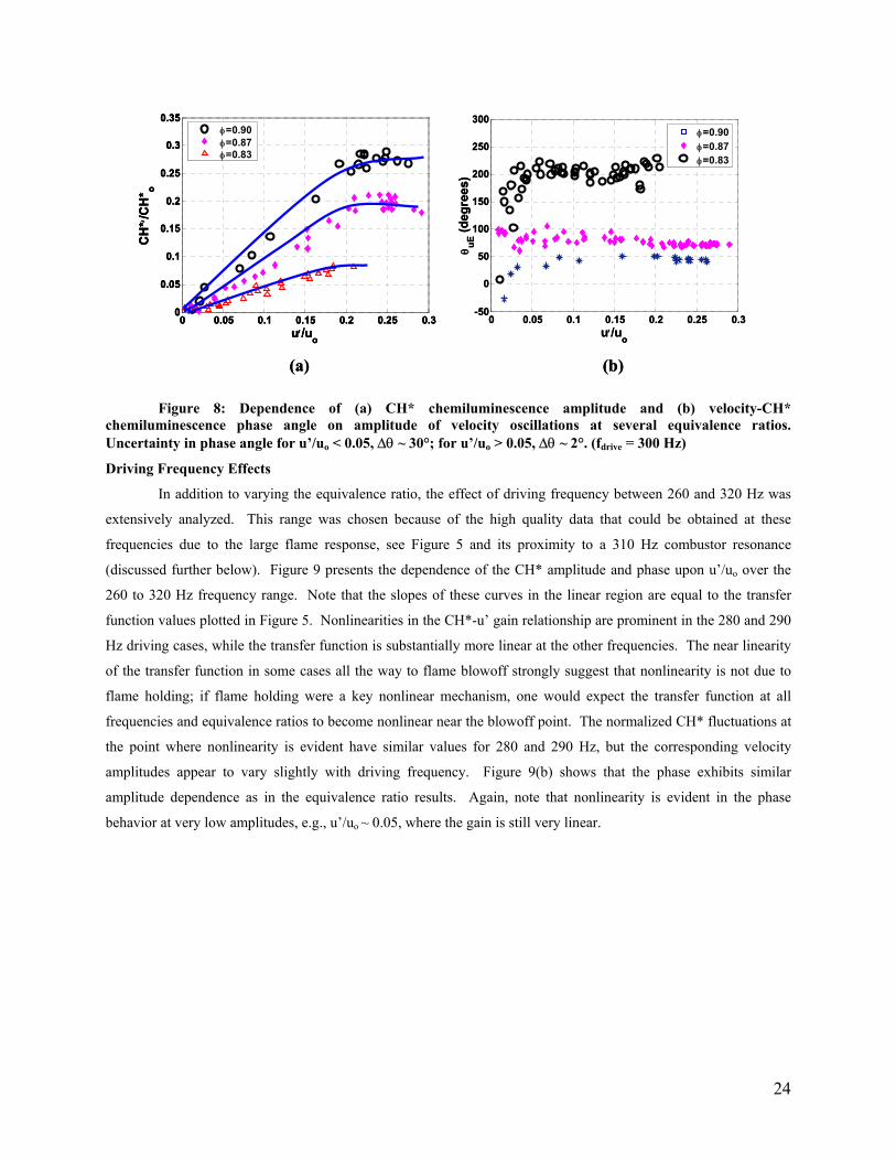
Figure 8: Dependence of (a) CH* chemiluminescence amplitude and (b) velocity-CH* chemiluminescence phase angle on amplitude of velocity oscillations at several equivalence ratios. Uncertainty in phase angle for u’/uo < 0.05, ∆θ ~ 30°; for u’/uo > 0.05, ∆θ ~ 2°. (fdrive = 300 Hz)
Driving Frequency Effects
In addition to varying the equivalence ratio, the effect of driving frequency between 260 and 320 Hz was
extensively analyzed. This range was chosen because of the high quality data that could be obtained at these
frequencies due to the large flame response, see Figure 5 and its proximity to a 310 Hz combustor resonance
(discussed further below). Figure 9 presents the dependence of the CH* amplitude and phase upon u’/uo over the
260 to 320 Hz frequency range. Note that the slopes of these curves in the linear region are equal to the transfer
function values plotted in Figure 5. Nonlinearities in the CH*-u’ gain relationship are prominent in the 280 and 290
Hz driving cases, while the transfer function is substantially more linear at the other frequencies. The near linearity
of the transfer function in some cases all the way to flame blowoff strongly suggest that nonlinearity is not due to
flame holding; if flame holding were a key nonlinear mechanism, one would expect the transfer function at all
frequencies and equivalence ratios to become nonlinear near the blowoff point. The normalized CH* fluctuations at
the point where nonlinearity is evident have similar values for 280 and 290 Hz, but the corresponding velocity
amplitudes appear to vary slightly with driving frequency. Figure 9(b) shows that the phase exhibits similar
amplitude dependence as in the equivalence ratio results. Again, note that nonlinearity is evident in the phase
behavior at very low amplitudes, e.g., u’/uo ~ 0.05, where the gain is still very linear.
24
u /uo
(a) (b)
u /uo
(a) (b)
u /uo
(a) (b)
u /uo
(a) (b)
Figure 9: Dependence of CH* chemiluminescence (a) amplitude and (b) phase upon velocity amplitude at several driving frequencies. Uncertainty in phase angle for u’/uo < 0.05, ∆θ ~ 30°; for u’/uo > 0.05, ∆θ ~ 2°. (φ = 0.95)
Harmonic and Subharmonic Characteristics
In addition to characterizing the dependence of the flame transfer function on the fundamental driving
frequency, extensive analysis of the higher and sub-harmonics of the dynamic signals was performed. Prior studies
suggest that such data are needed to obtain a comprehensive understanding of the nonlinear combustion process.
For example, it is well established from forced response studies in various mixing layers, jets, and wakes that such
understanding is key to the system’s nonlinear dynamics (e.g., see Ref. [33]). These amplitudes are substantially
smaller than those of the fundamental, however, resulting in reduced coherence between the fundamental and first
harmonic, γi=f,j=2f. As such, only a single subharmonic and harmonic of the chemiluminescence signal (CH*’f=fdrive/2
and CH*’f=2fdrive) could be accurately quantified. The first subharmonic as well as the first and second harmonics of
the pressure signal could be quantified due to much higher coherence values. While the presence of higher
harmonics in the data could be either to actuator or combustion process nonlinearities, analysis of our data indicates
that the dominant source of harmonic generation can be attributed to the nonlinear combustion process.
First harmonic characteristics of the CH* oscillations are presented in Figure 10 for two equivalence ratios,
φ = 0.95 and φ = 0.90 at a driving frequency of 300 Hz. These two cases present examples where the flame transfer
function remained linear throughout the range of disturbance amplitudes as well as where the flame transfer function
saturated at large amplitudes of velocity oscillations. Figure 10 illustrates that the first harmonic behavior can
change markedly between linear and nonlinear cases. For the linear case, φ = 0.95, the first harmonic of the
chemiluminescence exhibits a quadratic behavior on the fundamental throughout. This result is indicative of the
other cases where the transfer function remains linear. For nonlinear cases, however, the functional relationship
between the first harmonic and the fundamental changes. At low disturbance amplitudes, the general quadratic
behavior is followed for φ = 0.90. At forcing amplitudes above the saturation point of the fundamental, however,
the first harmonic has been found to exhibit a variety of behaviors. For φ = 0.90, the first harmonic deviates from
the quadratic dependence, by increasing much more rapidly. In other cases, the first harmonic increases more
25
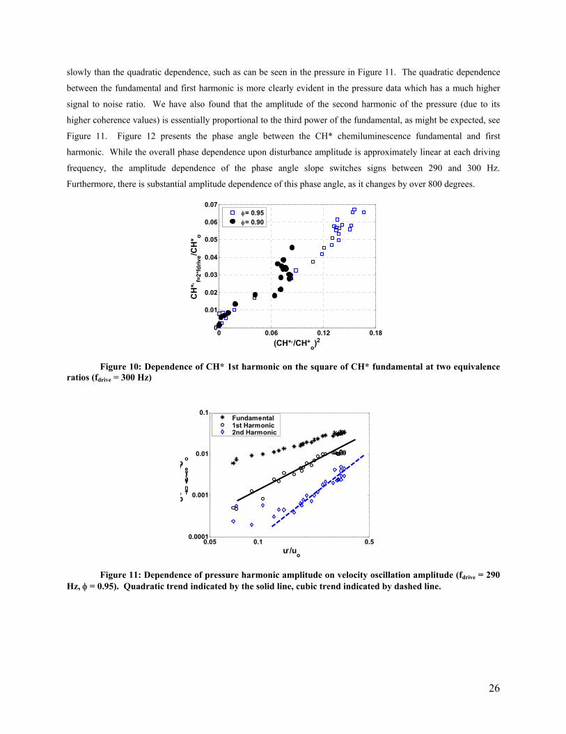
slowly than the quadratic dependence, such as can be seen in the pressure in Figure 11. The quadratic dependence
between the fundamental and first harmonic is more clearly evident in the pressure data which has a much higher
signal to noise ratio. We have also found that the amplitude of the second harmonic of the pressure (due to its
higher coherence values) is essentially proportional to the third power of the fundamental, as might be expected, see
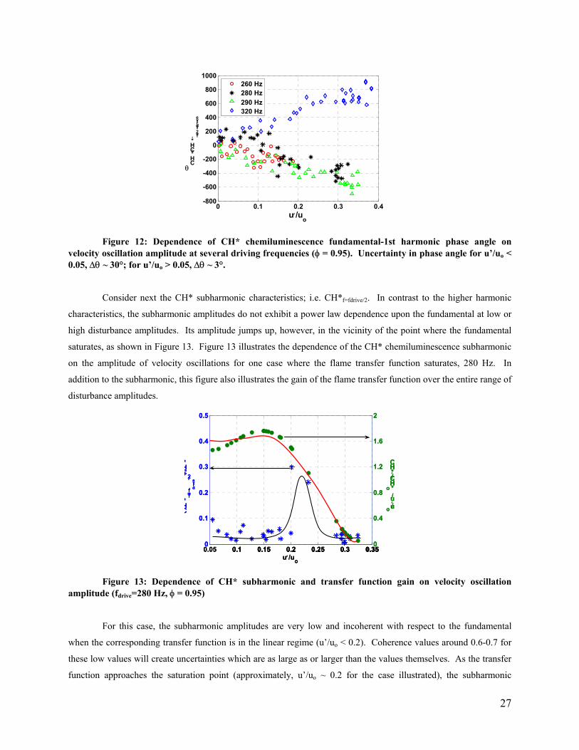
Figure 11. Figure 12 presents the phase angle between the CH* chemiluminescence fundamental and first
harmonic. While the overall phase dependence upon disturbance amplitude is approximately linear at each driving
frequency, the amplitude dependence of the phase angle slope switches signs between 290 and 300 Hz.
Furthermore, there is substantial amplitude dependence of this phase angle, as it changes by over 800 degrees.
0 0.06 0.12 0.180
0.01
0.02
0.03
0.04
0.05
0.06
0.07
(CH*′/CH*o)2
CH
* ′ f=2*
fdriv
e/CH
* o
φ= 0.95φ= 0.90
Figure 10: Dependence of CH* 1st harmonic on the square of CH* fundamental at two equivalence ratios (fdrive = 300 Hz)
0.05 0.1 0.50.0001
0.001
0.01
0.1
u′/uo
p′f=n*fdrive/po
Fundamental1st Harmonic2nd Harmonic
Figure 11: Dependence of pressure harmonic amplitude on velocity oscillation amplitude (fdrive = 290 Hz, φ = 0.95). Quadratic trend indicated by the solid line, cubic trend indicated by dashed line.
26
0 0.1 0.2 0.3 0.4-800
-600
-400
-200
0
200
400
600
800
1000
u′/uo
θCH*′CH*′
f=2*fdrive
260 Hz280 Hz290 Hz320 Hz
Figure 12: Dependence of CH* chemiluminescence fundamental-1st harmonic phase angle on velocity oscillation amplitude at several driving frequencies (φ = 0.95). Uncertainty in phase angle for u’/uo < 0.05, ∆θ ~ 30°; for u’/uo > 0.05, ∆θ ~ 3°.
Consider next the CH* subharmonic characteristics; i.e. CH*f=fdrive/2. In contrast to the higher harmonic
characteristics, the subharmonic amplitudes do not exhibit a power law dependence upon the fundamental at low or
high disturbance amplitudes. Its amplitude jumps up, however, in the vicinity of the point where the fundamental
saturates, as shown in Figure 13. Figure 13 illustrates the dependence of the CH* chemiluminescence subharmonic
on the amplitude of velocity oscillations for one case where the flame transfer function saturates, 280 Hz. In
addition to the subharmonic, this figure also illustrates the gain of the flame transfer function over the entire range of
disturbance amplitudes.
0.05 0.1 0.15 0.2 0.25 0.3 0.350
0.1
0.2
0.3
0.4
0.5
CH*
f=f dr
ive/2/C
H*
0.1 0.15 0.2 0.25 0.3 0.350
0.4
0.8
1.2
1.6
2
u′/uo
CH*′/CH*o / u′/uo
0.05 0.1 0.15 0.2 0.25 0.3 0.350
0.1
0.2
0.3
0.4
0.5
CH*
f=f dr
ive/2/C
H*
0.1 0.15 0.2 0.25 0.3 0.350
0.4
0.8
1.2
1.6
2
u′/uo
CH*′/CH*o / u′/uo
Figure 13: Dependence of CH* subharmonic and transfer function gain on velocity oscillation amplitude (fdrive=280 Hz, φ = 0.95)
For this case, the subharmonic amplitudes are very low and incoherent with respect to the fundamental
when the corresponding transfer function is in the linear regime (u’/uo < 0.2). Coherence values around 0.6-0.7 for
these low values will create uncertainties which are as large as or larger than the values themselves. As the transfer
function approaches the saturation point (approximately, u’/uo ~ 0.2 for the case illustrated), the subharmonic
27
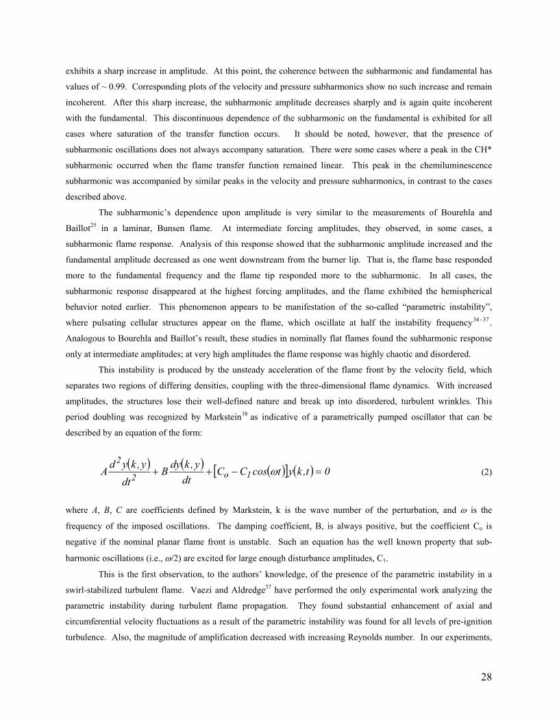
exhibits a sharp increase in amplitude. At this point, the coherence between the subharmonic and fundamental has
values of ~ 0.99. Corresponding plots of the velocity and pressure subharmonics show no such increase and remain
incoherent. After this sharp increase, the subharmonic amplitude decreases sharply and is again quite incoherent
with the fundamental. This discontinuous dependence of the subharmonic on the fundamental is exhibited for all
cases where saturation of the transfer function occurs. It should be noted, however, that the presence of
subharmonic oscillations does not always accompany saturation. There were some cases where a peak in the CH*
subharmonic occurred when the flame transfer function remained linear. This peak in the chemiluminescence
subharmonic was accompanied by similar peaks in the velocity and pressure subharmonics, in contrast to the cases
described above.
The subharmonic’s dependence upon amplitude is very similar to the measurements of Bourehla and
Baillot25 in a laminar, Bunsen flame. At intermediate forcing amplitudes, they observed, in some cases, a
subharmonic flame response. Analysis of this response showed that the subharmonic amplitude increased and the
fundamental amplitude decreased as one went downstream from the burner lip. That is, the flame base responded
more to the fundamental frequency and the flame tip responded more to the subharmonic. In all cases, the
subharmonic response disappeared at the highest forcing amplitudes, and the flame exhibited the hemispherical
behavior noted earlier. This phenomenon appears to be manifestation of the so-called “parametric instability”,
where pulsating cellular structures appear on the flame, which oscillate at half the instability frequency34 - 37 .
Analogous to Bourehla and Baillot’s result, these studies in nominally flat flames found the subharmonic response
only at intermediate amplitudes; at very high amplitudes the flame response was highly chaotic and disordered.
This instability is produced by the unsteady acceleration of the flame front by the velocity field, which
separates two regions of differing densities, coupling with the three-dimensional flame dynamics. With increased
amplitudes, the structures lose their well-defined nature and break up into disordered, turbulent wrinkles. This
period doubling was recognized by Markstein38 as indicative of a parametrically pumped oscillator that can be
described by an equation of the form:
( ) ( ) ( )[ ] ( ) 0t,kytcosCCdt
y,kdyBdt
y,kydA 1o2
2=−++ ω (2)
where A, B, C are coefficients defined by Markstein, k is the wave number of the perturbation, and ω is the
frequency of the imposed oscillations. The damping coefficient, B, is always positive, but the coefficient Co is
negative if the nominal planar flame front is unstable. Such an equation has the well known property that sub-
harmonic oscillations (i.e., ω/2) are excited for large enough disturbance amplitudes, C1.
This is the first observation, to the authors’ knowledge, of the presence of the parametric instability in a
swirl-stabilized turbulent flame. Vaezi and Aldredge37 have performed the only experimental work analyzing the
parametric instability during turbulent flame propagation. They found substantial enhancement of axial and
circumferential velocity fluctuations as a result of the parametric instability was found for all levels of pre-ignition
turbulence. Also, the magnitude of amplification decreased with increasing Reynolds number. In our experiments,
28
the Reynolds number defined by the premixer exit diameter was substantially larger than those investigated by
Vaezi & Aldredge37. Analogous to their results, no sudden visible changes in the flame position, length, or shape
were noted before saturation of the transfer function occurred which indicate that turbulent flame speed
enhancement was minimal. However, it appears highly probable that nonlinear interactions between the flow
forcing and parametric instability (possibly through its impact on the fluctuating flame position) are responsible for
saturation of the flame response. This is evidenced by the fact that 1) the jump in subharmonic amplitude occurs at
essentially the same value as that at which saturation occurs, and 2) subharmonic oscillations are always present in
cases where saturation of the fundamental occur.
Atmospheric Swirl Stabilized Burner
INSTRUMENTATION AND EXPERIMENTAL FACILITY
This section describes the continuation of the nonlinear flame response experiments described in the
previous section. Instead of performing the experiments on the gas turbine combustor simulator (described in Figure
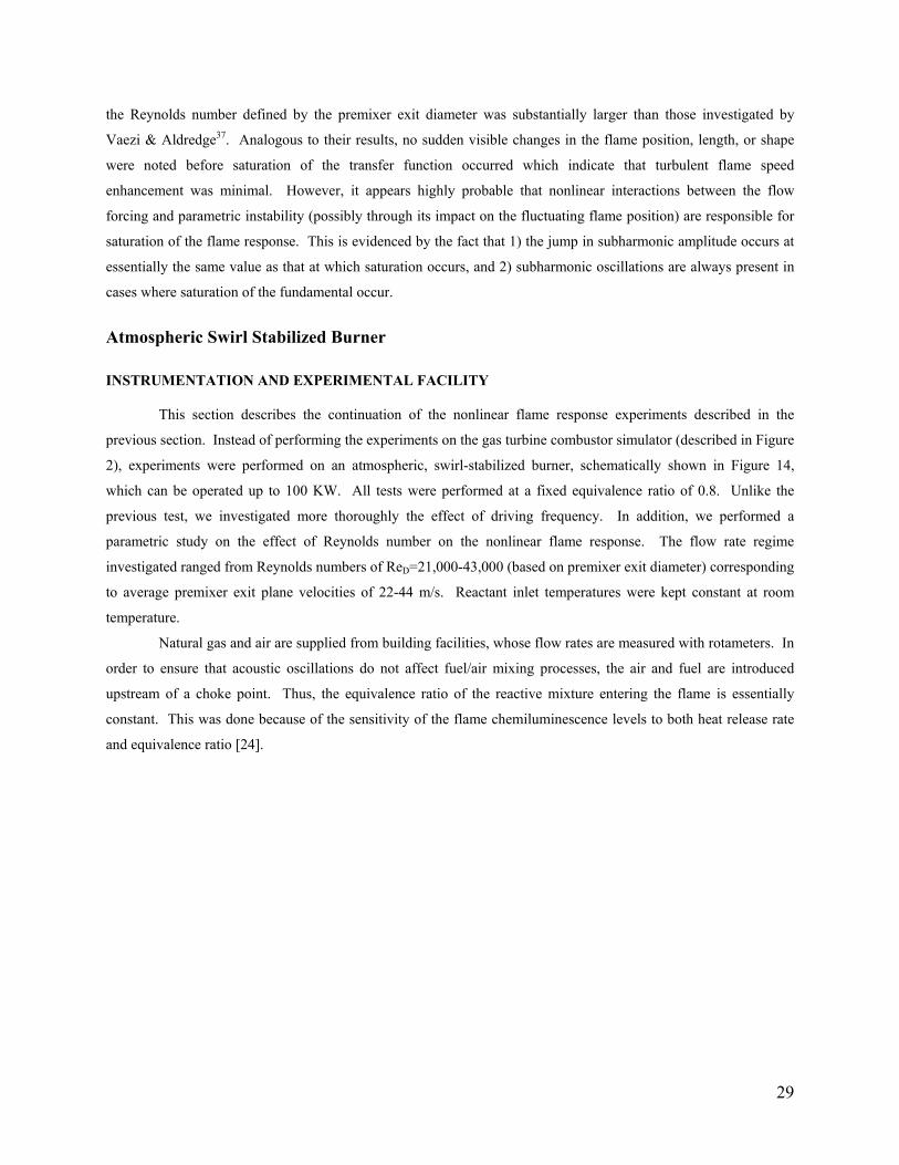
2), experiments were performed on an atmospheric, swirl-stabilized burner, schematically shown in Figure 14,
which can be operated up to 100 KW. All tests were performed at a fixed equivalence ratio of 0.8. Unlike the
previous test, we investigated more thoroughly the effect of driving frequency. In addition, we performed a
parametric study on the effect of Reynolds number on the nonlinear flame response. The flow rate regime
investigated ranged from Reynolds numbers of ReD=21,000-43,000 (based on premixer exit diameter) corresponding
to average premixer exit plane velocities of 22-44 m/s. Reactant inlet temperatures were kept constant at room
temperature.
Natural gas and air are supplied from building facilities, whose flow rates are measured with rotameters. In
order to ensure that acoustic oscillations do not affect fuel/air mixing processes, the air and fuel are introduced
upstream of a choke point. Thus, the equivalence ratio of the reactive mixture entering the flame is essentially
constant. This was done because of the sensitivity of the flame chemiluminescence levels to both heat release rate
and equivalence ratio [24].
29
Air + Natural Gas
Loudspeakers
Pressure Taps
Inlet Section
Combustion Zone
Air + Natural Gas
Loudspeakers
Pressure Taps
Inlet Section
Combustion Zone
Figure 14. Schematic of swirl-stabilized combustor
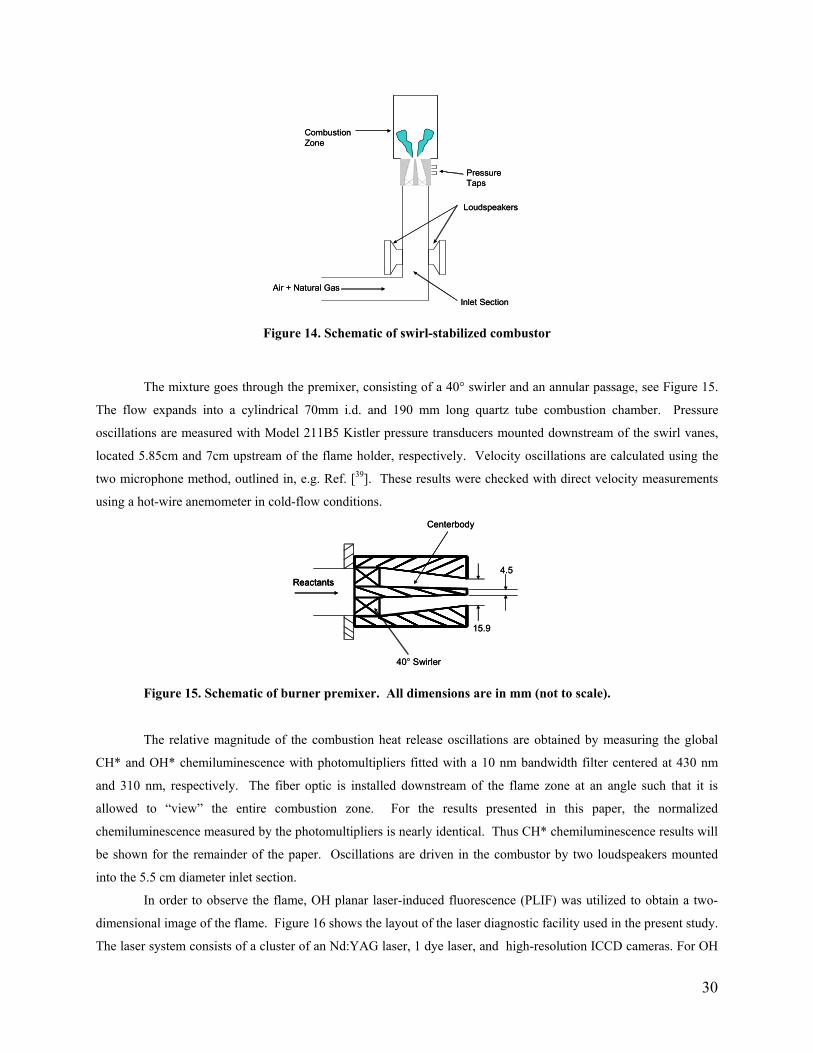
The mixture goes through the premixer, consisting of a 40° swirler and an annular passage, see Figure 15.
The flow expands into a cylindrical 70mm i.d. and 190 mm long quartz tube combustion chamber. Pressure
oscillations are measured with Model 211B5 Kistler pressure transducers mounted downstream of the swirl vanes,
located 5.85cm and 7cm upstream of the flame holder, respectively. Velocity oscillations are calculated using the
two microphone method, outlined in, e.g. Ref. [39]. These results were checked with direct velocity measurements
using a hot-wire anemometer in cold-flow conditions.
Reactants4.5
15.9
40° Swirler
Centerbody
ReactantsReactants4.5
15.9
40° Swirler
Centerbody
Figure 15. Schematic of burner premixer. All dimensions are in mm (not to scale).
The relative magnitude of the combustion heat release oscillations are obtained by measuring the global
CH* and OH* chemiluminescence with photomultipliers fitted with a 10 nm bandwidth filter centered at 430 nm
and 310 nm, respectively. The fiber optic is installed downstream of the flame zone at an angle such that it is
allowed to “view” the entire combustion zone. For the results presented in this paper, the normalized
chemiluminescence measured by the photomultipliers is nearly identical. Thus CH* chemiluminescence results will
be shown for the remainder of the paper. Oscillations are driven in the combustor by two loudspeakers mounted
into the 5.5 cm diameter inlet section.
In order to observe the flame, OH planar laser-induced fluorescence (PLIF) was utilized to obtain a two-
dimensional image of the flame. Figure 16 shows the layout of the laser diagnostic facility used in the present study.
The laser system consists of a cluster of an Nd:YAG laser, 1 dye laser, and high-resolution ICCD cameras. For OH
30
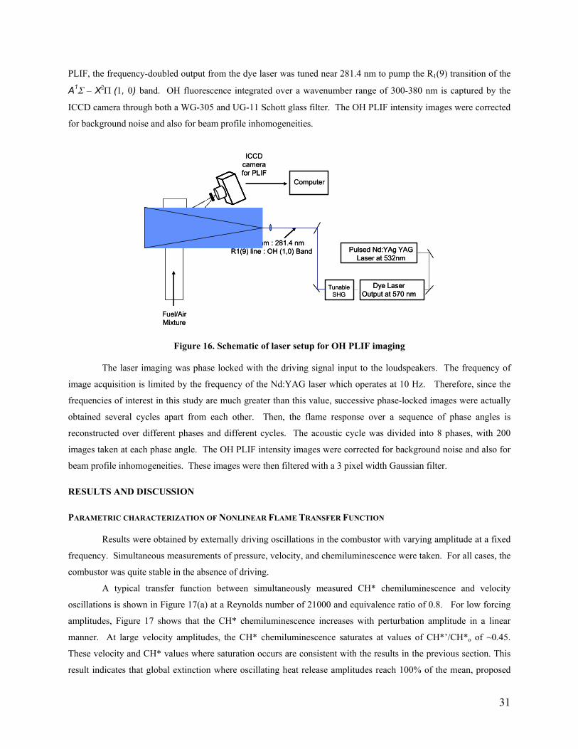
PLIF, the frequency-doubled output from the dye laser was tuned near 281.4 nm to pump the R1(9) transition of the
A1Σ – X2Π (1, 0) band. OH fluorescence integrated over a wavenumber range of 300-380 nm is captured by the
ICCD camera through both a WG-305 and UG-11 Schott glass filter. The OH PLIF intensity images were corrected
for background noise and also for beam profile inhomogeneities.
Dye LaserOutput at 570 nm
Tunable SHG
UV Beam : 281.4 nmR1(9) line : OH (1,0) Band Pulsed Nd:YAg YAG
Laser at 532nm
ICCDcamerafor PLIF
Computer
Fuel/Air Mixture
Dye LaserOutput at 570 nm
Tunable SHG
UV Beam : 281.4 nmR1(9) line : OH (1,0) Band Pulsed Nd:YAg YAG
Laser at 532nm
ICCDcamerafor PLIF
Computer
Fuel/Air Mixture
Figure 16. Schematic of laser setup for OH PLIF imaging
The laser imaging was phase locked with the driving signal input to the loudspeakers. The frequency of
image acquisition is limited by the frequency of the Nd:YAG laser which operates at 10 Hz. Therefore, since the
frequencies of interest in this study are much greater than this value, successive phase-locked images were actually
obtained several cycles apart from each other. Then, the flame response over a sequence of phase angles is
reconstructed over different phases and different cycles. The acoustic cycle was divided into 8 phases, with 200
images taken at each phase angle. The OH PLIF intensity images were corrected for background noise and also for
beam profile inhomogeneities. These images were then filtered with a 3 pixel width Gaussian filter.
RESULTS AND DISCUSSION
PARAMETRIC CHARACTERIZATION OF NONLINEAR FLAME TRANSFER FUNCTION
Results were obtained by externally driving oscillations in the combustor with varying amplitude at a fixed
frequency. Simultaneous measurements of pressure, velocity, and chemiluminescence were taken. For all cases, the
combustor was quite stable in the absence of driving.
A typical transfer function between simultaneously measured CH* chemiluminescence and velocity
oscillations is shown in Figure 17(a) at a Reynolds number of 21000 and equivalence ratio of 0.8. For low forcing
amplitudes, Figure 17 shows that the CH* chemiluminescence increases with perturbation amplitude in a linear
manner. At large velocity amplitudes, the CH* chemiluminescence saturates at values of CH*’/CH*o of ~0.45.
These velocity and CH* values where saturation occurs are consistent with the results in the previous section. This
result indicates that global extinction where oscillating heat release amplitudes reach 100% of the mean, proposed
31
theoretically by Dowling [16], is not an important mechanism at this condition. Figure 17(b) presents the
corresponding u’-CH*’ phase relationship. The phase relationship exhibits a complex amplitude dependence on the
amplitude of velocity oscillations. The phase angle changes by nearly 50 degrees while the transfer function
remains linear. The sharp decrease in phase angle at u’/uo ~0.45 occurs after the CH*’/CH*o value saturates.
Figure 18(a) presents transfer function results for driving frequencies between 130-150 Hz at a Reynolds
number of 21000. Figure 18 illustrates that the transfer function at 130 Hz and 140 Hz remains linear up to
CH*’/CH*o values near 0.95 before saturating. Thus, the saturation amplitude here is substantially higher than that
in Figure 17, illustrating the substantial dependence of saturation amplitude upon flow conditions and disturbance
frequency. Note that the saturation amplitude here is quite close to 100%, suggesting a global extinction type
mechanism as proposed by Dowling [16]. Figure 18(b) presents the corresponding u’-CH*’ phase. Similar to the
comparison between the saturation amplitudes between the cases at 210 and 130 Hz, the phase angle shapes for
these two frequencies are also quite different. The phase angle at these frequencies exhibits significant amplitude
dependence at velocity oscillation amplitudes where the gain of the transfer function remains in the linear regime.
This effect is again consistent with the results in the previous section. The phase angle is seen to almost saturate as
well and remain relatively constant around 85-90 degrees over nearly 50% of the velocity amplitude range.
Both Figure 17 and Figure 18 illustrate typical shapes of transfer functions that have been observed
experimentally and proposed theoretically. For low velocity amplitudes, the corresponding heat release oscillations
increase linearly. At the largest velocity amplitudes, the heat release fluctuations saturate. However, more complex
amplitude dependencies were observed at other conditions. Figure 19 shows two such cases, obtained at 340 and
410 Hz, respectively. Both curves show that the CH* chemiluminescence increases linearly with increasing velocity
oscillation amplitudes at low values of driving. At 340 Hz, the CH* oscillation amplitude begins to saturate at
values around 0.65-0.7 of the mean value. However, instead of remaining nearly constant, with further increases in
excitation amplitude the response increases again. In a similar manner, for 410 Hz, Figure 19 shows that the transfer
function begins to saturate at a CH*’/CH*o value of 0.35. Similar to the 340 Hz case, the flame response begins to
increase again before saturating again at CH*’/CH*o value of nearly 0.6. This trend is similar to the experimental
results of Balachandran et al. for a bluff-body stabilized flame without swirl [26].
32
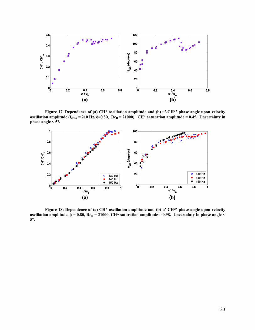
0 0.2 0.4 0.6 0.80
0.1
0.2
0.3
0.4
0.5
u′ / uo
CH
* ′ / C
H* o
(a) (b)
0 0.2 0.4 0.6 0.80
20
40
60
80
100
120
u′ / uo
θ uE (d
egre
es)
0 0.2 0.4 0.6 0.80
0.1
0.2
0.3
0.4
0.5
u′ / uo
CH
* ′ / C
H* o
(a) (b)
0 0.2 0.4 0.6 0.80
20
40
60
80
100
120
u′ / uo
θ uE (d
egre
es)
Figure 17. Dependence of (a) CH* oscillation amplitude and (b) u’-CH*’ phase angle upon velocity oscillation amplitude (fdrive = 210 Hz, φ=0.80, ReD = 21000). CH* saturation amplitude = 0.45. Uncertainty in phase angle < 5°.
0 0.2 0.4 0.6 0.8 10
0.2
0.4
0.6
0.8
1
u′/uo
CH
* ′/C
H* o
130 Hz140 Hz150 Hz
(a) (b)
0 0.2 0.4 0.6 0.8 10
20
40
60
80
100
u′ / uo
θ uE (d
egre
es)
130 Hz140 Hz150 Hz
0 0.2 0.4 0.6 0.8 10
0.2
0.4
0.6
0.8
1
u′/uo
CH
* ′/C
H* o
130 Hz140 Hz150 Hz
(a) (b)
0 0.2 0.4 0.6 0.8 10
20
40
60
80
100
u′ / uo
θ uE (d
egre
es)
130 Hz140 Hz150 Hz
Figure 18: Dependence of (a) CH* oscillation amplitude and (b) u’-CH*’ phase angle upon velocity oscillation amplitude, φ = 0.80, ReD = 21000. CH* saturation amplitude ~ 0.98. Uncertainty in phase angle < 5°.
33
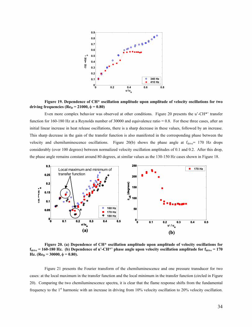
0 0.2 0.4 0.6 0.80
0.1
0.2
0.3
0.4
0.5
0.6
0.7
0.8
0.9
u′/uo
CH*′/CH* o
340 Hz410 Hz
Figure 19. Dependence of CH* oscillation amplitude upon amplitude of velocity oscillations for two driving frequencies (ReD = 21000, φ = 0.80)
Even more complex behavior was observed at other conditions. Figure 20 presents the u’-CH*’ transfer
function for 160-180 Hz at a Reynolds number of 30000 and equivalence ratio = 0.8. For these three cases, after an
initial linear increase in heat release oscillations, there is a sharp decrease in these values, followed by an increase.
This sharp decrease in the gain of the transfer function is also manifested in the corresponding phase between the
velocity and chemiluminescence oscillations. Figure 20(b) shows the phase angle at fdrive= 170 Hz drops
considerably (over 100 degrees) between normalized velocity oscillation amplitudes of 0.1 and 0.2. After this drop,
the phase angle remains constant around 80 degrees, at similar values as the 130-150 Hz cases shown in Figure 18.
0 0.1 0.2 0.3 0.4 0.50
0.05
0.1
0.15
0.2
0.25
0.3
u′/uo
CH*′ / CH* o
160 Hz170 Hz180 Hz
Local maximum and minimum of transfer function
(a) (b)
0 0.1 0.2 0.3 0.4 0.50
50
100
150
200
250
u′ / uo
θ uE (d
egre
es)
170 Hz
0 0.1 0.2 0.3 0.4 0.50
0.05
0.1
0.15
0.2
0.25
0.3
u′/uo
CH*′ / CH* o
160 Hz170 Hz180 Hz
Local maximum and minimum of transfer function
0 0.1 0.2 0.3 0.4 0.50
0.05
0.1
0.15
0.2
0.25
0.3
u′/uo
CH*′ / CH* o
160 Hz170 Hz180 Hz
Local maximum and minimum of transfer function
(a) (b)
0 0.1 0.2 0.3 0.4 0.50
50
100
150
200
250
u′ / uo
θ uE (d
egre
es)
170 Hz
Figure 20. (a) Dependence of CH* oscillation amplitude upon amplitude of velocity oscillations for fdrive = 160-180 Hz. (b) Dependence of u’-CH*’ phase angle upon velocity oscillation amplitude for fdrive = 170 Hz. (ReD = 30000, φ = 0.80).
Figure 21 presents the Fourier transform of the chemiluminescence and one pressure transducer for two
cases: at the local maximum in the transfer function and the local minimum in the transfer function (circled in Figure
20). Comparing the two chemiluminescence spectra, it is clear that the flame response shifts from the fundamental
frequency to the 1st harmonic with an increase in driving from 10% velocity oscillation to 20% velocity oscillation.
34
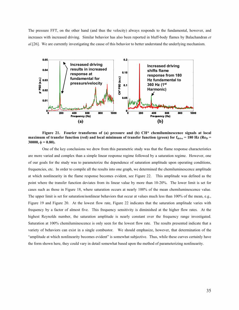
The pressure FFT, on the other hand (and thus the velocity) always responds to the fundamental, however, and
increases with increased driving. Similar behavior has also been reported in bluff-body flames by Balachandran et
al.[26]. We are currently investigating the cause of this behavior to better understand the underlying mechanism.
0 200 400 600 800 10000
0.05
0.1
0.15
0.2
Frequency (Hz)C
H* P
SD (a
.u.)
Increased driving shifts flame response from 180 Hz fundamental to 360 Hz (1st
Harmonic)
0 200 400 600 800 10000
0.01
0.02
0.03
0.04
0.05
Frequency (Hz)
p ′ P
SD
(a.u
.)
Increased driving results in increased response at fundamental for pressure/velocity
(a) (b)
0 200 400 600 800 10000
0.05
0.1
0.15
0.2
Frequency (Hz)C
H* P
SD (a
.u.)
Increased driving shifts flame response from 180 Hz fundamental to 360 Hz (1st
Harmonic)
0 200 400 600 800 10000
0.05
0.1
0.15
0.2
Frequency (Hz)C
H* P
SD (a
.u.)
Increased driving shifts flame response from 180 Hz fundamental to 360 Hz (1st
Harmonic)
0 200 400 600 800 10000
0.01
0.02
0.03
0.04
0.05
Frequency (Hz)
p ′ P
SD
(a.u
.)
Increased driving results in increased response at fundamental for pressure/velocity
0 200 400 600 800 10000
0.01
0.02
0.03
0.04
0.05
Frequency (Hz)
p ′ P
SD
(a.u
.)
Increased driving results in increased response at fundamental for pressure/velocity
(a) (b)
Figure 21. Fourier transforms of (a) pressure and (b) CH* chemiluminescence signals at local maximum of transfer function (red) and local minimum of transfer function (green) for fdrive = 180 Hz (ReD = 30000, φ = 0.80).
One of the key conclusions we drew from this parametric study was that the flame response characteristics
are more varied and complex than a simple linear response regime followed by a saturation regime. However, one
of our goals for the study was to parameterize the dependence of saturation amplitude upon operating conditions,
frequencies, etc. In order to compile all the results into one graph, we determined the chemiluminescence amplitude
at which nonlinearity in the flame response becomes evident, see Figure 22. This amplitude was defined as the
point where the transfer function deviates from its linear value by more than 10-20%. The lower limit is set for
cases such as those in Figure 18, where saturation occurs at nearly 100% of the mean chemiluminescence value.
The upper limit is set for saturation/nonlinear behaviors that occur at values much less than 100% of the mean, e.g.,
Figure 19 and Figure 20. At the lowest flow rate, Figure 22 indicates that the saturation amplitude varies with
frequency by a factor of almost five. This frequency sensitivity is diminished at the higher flow rates. At the
highest Reynolds number, the saturation amplitude is nearly constant over the frequency range investigated.
Saturation at 100% chemiluminescence is only seen for the lowest flow rate. The results presented indicate that a
variety of behaviors can exist in a single combustor. We should emphasize, however, that determination of the
“amplitude at which nonlinearity becomes evident” is somewhat subjective. Thus, while these curves certainly have
the form shown here, they could vary in detail somewhat based upon the method of parameterizing nonlinearity.
35
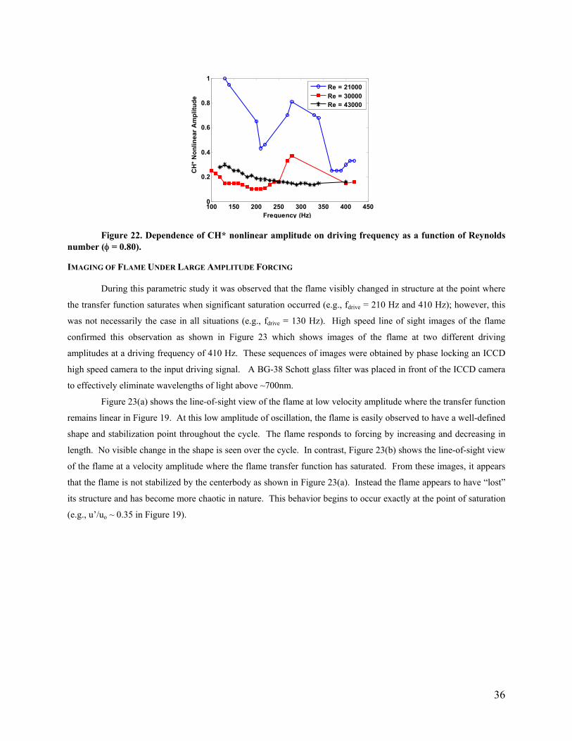
100 150 200 250 300 350 400 4500
0.2
0.4
0.6
0.8
1
Frequency (Hz)
CH
* Non
linea
r Am
plitu
de
Re = 21000Re = 30000Re = 43000
Figure 22. Dependence of CH* nonlinear amplitude on driving frequency as a function of Reynolds number (φ = 0.80).
IMAGING OF FLAME UNDER LARGE AMPLITUDE FORCING
During this parametric study it was observed that the flame visibly changed in structure at the point where
the transfer function saturates when significant saturation occurred (e.g., fdrive = 210 Hz and 410 Hz); however, this
was not necessarily the case in all situations (e.g., fdrive = 130 Hz). High speed line of sight images of the flame
confirmed this observation as shown in Figure 23 which shows images of the flame at two different driving
amplitudes at a driving frequency of 410 Hz. These sequences of images were obtained by phase locking an ICCD
high speed camera to the input driving signal. A BG-38 Schott glass filter was placed in front of the ICCD camera
to effectively eliminate wavelengths of light above ~700nm.
Figure 23(a) shows the line-of-sight view of the flame at low velocity amplitude where the transfer function
remains linear in Figure 19. At this low amplitude of oscillation, the flame is easily observed to have a well-defined
shape and stabilization point throughout the cycle. The flame responds to forcing by increasing and decreasing in
length. No visible change in the shape is seen over the cycle. In contrast, Figure 23(b) shows the line-of-sight view
of the flame at a velocity amplitude where the flame transfer function has saturated. From these images, it appears
that the flame is not stabilized by the centerbody as shown in Figure 23(a). Instead the flame appears to have “lost”
its structure and has become more chaotic in nature. This behavior begins to occur exactly at the point of saturation
(e.g., u’/uo ~ 0.35 in Figure 19).
36
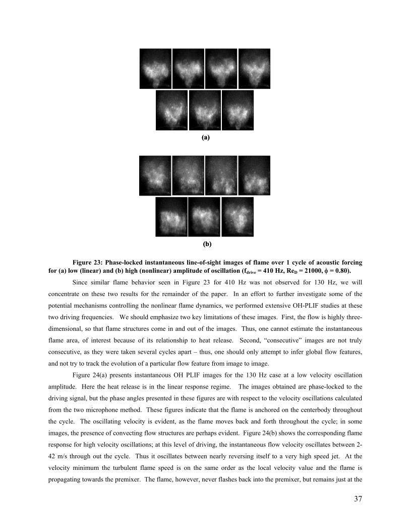
(a)
(b)
(a)
(b)
Figure 23: Phase-locked instantaneous line-of-sight images of flame over 1 cycle of acoustic forcing for (a) low (linear) and (b) high (nonlinear) amplitude of oscillation (fdrive = 410 Hz, ReD = 21000, φ = 0.80).
Since similar flame behavior seen in Figure 23 for 410 Hz was not observed for 130 Hz, we will
concentrate on these two results for the remainder of the paper. In an effort to further investigate some of the
potential mechanisms controlling the nonlinear flame dynamics, we performed extensive OH-PLIF studies at these
two driving frequencies. We should emphasize two key limitations of these images. First, the flow is highly three-
dimensional, so that flame structures come in and out of the images. Thus, one cannot estimate the instantaneous
flame area, of interest because of its relationship to heat release. Second, “consecutive” images are not truly
consecutive, as they were taken several cycles apart – thus, one should only attempt to infer global flow features,
and not try to track the evolution of a particular flow feature from image to image.
Figure 24(a) presents instantaneous OH PLIF images for the 130 Hz case at a low velocity oscillation
amplitude. Here the heat release is in the linear response regime. The images obtained are phase-locked to the
driving signal, but the phase angles presented in these figures are with respect to the velocity oscillations calculated
from the two microphone method. These figures indicate that the flame is anchored on the centerbody throughout
the cycle. The oscillating velocity is evident, as the flame moves back and forth throughout the cycle; in some
images, the presence of convecting flow structures are perhaps evident. Figure 24(b) shows the corresponding flame
response for high velocity oscillations; at this level of driving, the instantaneous flow velocity oscillates between 2-
42 m/s through out the cycle. Thus it oscillates between nearly reversing itself to a very high speed jet. At the
velocity minimum the turbulent flame speed is on the same order as the local velocity value and the flame is
propagating towards the premixer. The flame, however, never flashes back into the premixer, but remains just at the
37
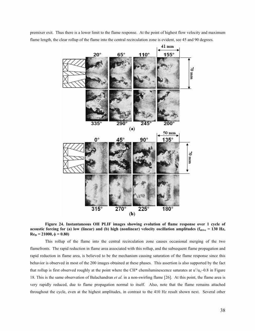
premixer exit. Thus there is a lower limit to the flame response. At the point of highest flow velocity and maximum
flame length, the clear rollup of the flame into the central recirculation zone is evident, see 45 and 90 degrees.
Figure 24. Instantaneous OH PLIF images showing evolution of flame response over 1 cycle of acoustic forcing for (a) low (linear) and (b) high (nonlinear) velocity oscillation amplitudes (fdrive = 130 Hz, ReD = 21000, φ = 0.80)
This rollup of the flame into the central recirculation zone causes occasional merging of the two
flamefronts. The rapid reduction in flame area associated with this rollup, and the subsequent flame propagation and
rapid reduction in flame area, is believed to be the mechanism causing saturation of the flame response since this
behavior is observed in most of the 200 images obtained at these phases. This assertion is also supported by the fact
that rollup is first observed roughly at the point where the CH* chemiluminescence saturates at u’/uo~0.8 in Figure
18. This is the same observation of Balachandran et al. in a non-swirling flame [26]. At this point, the flame area is
very rapidly reduced, due to flame propagation normal to itself. Also, note that the flame remains attached
throughout the cycle, even at the highest amplitudes, in contrast to the 410 Hz result shown next. Several other
38
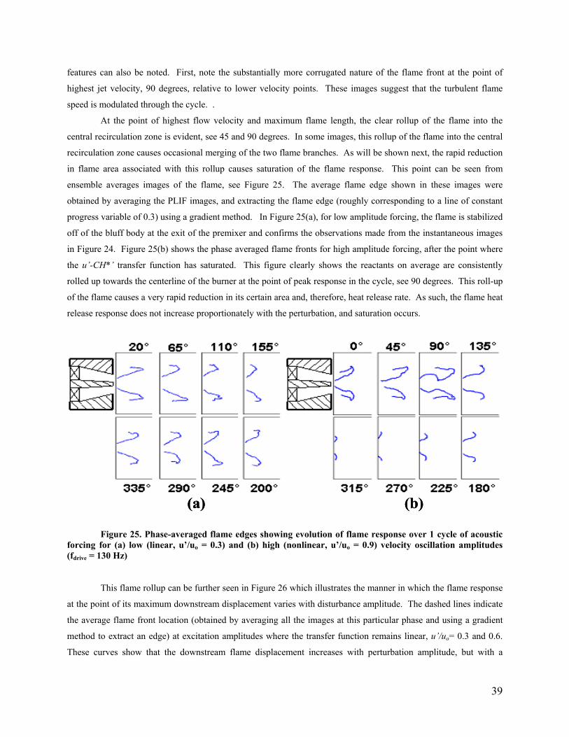
features can also be noted. First, note the substantially more corrugated nature of the flame front at the point of
highest jet velocity, 90 degrees, relative to lower velocity points. These images suggest that the turbulent flame
speed is modulated through the cycle. .
At the point of highest flow velocity and maximum flame length, the clear rollup of the flame into the
central recirculation zone is evident, see 45 and 90 degrees. In some images, this rollup of the flame into the central
recirculation zone causes occasional merging of the two flame branches. As will be shown next, the rapid reduction
in flame area associated with this rollup causes saturation of the flame response. This point can be seen from
ensemble averages images of the flame, see Figure 25. The average flame edge shown in these images were
obtained by averaging the PLIF images, and extracting the flame edge (roughly corresponding to a line of constant
progress variable of 0.3) using a gradient method. In Figure 25(a), for low amplitude forcing, the flame is stabilized
off of the bluff body at the exit of the premixer and confirms the observations made from the instantaneous images
in Figure 24. Figure 25(b) shows the phase averaged flame fronts for high amplitude forcing, after the point where
the u’-CH*’ transfer function has saturated. This figure clearly shows the reactants on average are consistently
rolled up towards the centerline of the burner at the point of peak response in the cycle, see 90 degrees. This roll-up
of the flame causes a very rapid reduction in its certain area and, therefore, heat release rate. As such, the flame heat
release response does not increase proportionately with the perturbation, and saturation occurs.
(a) (b)(a) (b)
Figure 25. Phase-averaged flame edges showing evolution of flame response over 1 cycle of acoustic forcing for (a) low (linear, u’/uo = 0.3) and (b) high (nonlinear, u’/uo = 0.9) velocity oscillation amplitudes (fdrive = 130 Hz)
This flame rollup can be further seen in Figure 26 which illustrates the manner in which the flame response
at the point of its maximum downstream displacement varies with disturbance amplitude. The dashed lines indicate
the average flame front location (obtained by averaging all the images at this particular phase and using a gradient
method to extract an edge) at excitation amplitudes where the transfer function remains linear, u’/uo= 0.3 and 0.6.
These curves show that the downstream flame displacement increases with perturbation amplitude, but with a
39
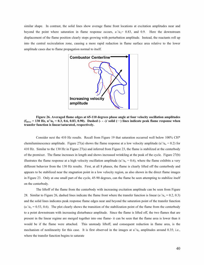
similar shape. In contrast, the solid lines show average flame front locations at excitation amplitudes near and
beyond the point where saturation in flame response occurs, u’/uo= 0.83, and 0.9. Here the downstream
displacement of the flame position clearly stops growing with perturbation amplitude. Instead, the reactants roll up
into the central recirculation zone, causing a more rapid reduction in flame surface area relative to the lower
amplitude cases due to flame propagation normal to itself.
Combustor Centerline
Increasing velocity amplitude
Combustor Centerline
Increasing velocity amplitude
Figure 26. Averaged flame edges at 65-110 degrees phase angle at four velocity oscillation amplitudes (fdrive = 130 Hz, u’/uo = 0.3, 0.6, 0.83, 0.90). Dashed (- - -)/ solid (___) lines indicate peak flame response when transfer function is linear/saturated, respectively.
Consider next the 410 Hz results. Recall from Figure 19 that saturation occurred well below 100% CH*
chemiluminescence amplitude. Figure 27(a) shows the flame response at a low velocity amplitude (u’/uo = 0.2) for
410 Hz. Similar to the 130 Hz in Figure 27(a) and inferred from Figure 23, the flame is stabilized at the centerbody
of the premixer. The flame increases in length and shows increased wrinkling at the peak of the cycle. Figure 27(b)
illustrates the flame response at a high velocity oscillation amplitude (u’/uo = 0.6), where the flame exhibits a very
different behavior from the 130 Hz results. First, at all 8 phases, the flame is clearly lifted off the centerbody and
appears to be stabilized near the stagnation point in a low velocity region, as also shown in the direct flame images
in Figure 23. Only at one small part of the cycle, 45-90 degrees, can the flame be seen attempting to stabilize itself
on the centerbody.
The liftoff of the flame from the centerbody with increasing excitation amplitude can be seen from Figure
28. Similar to Figure 26, dashed lines indicate the flame front where the transfer function is linear (u’/uo = 0.2, 0.3)
and the solid lines indicates peak response flame edges near and beyond the saturation point of the transfer function
(u’/uo = 0.53, 0.6). The plot clearly shows the transition of the stabilization point of the flame from the centerbody
to a point downstream with increasing disturbance amplitude. Since the flame is lifted off, the two flames that are
present in the linear regime are merged together into one flame- it can be seen that the flame area is lower than it
would be if the flame were attached. This unsteady liftoff, and consequent reduction in flame area, is the
mechanism of nonlinearity for this case. It is first observed in the images at u’/uo amplitudes around 0.35; i.e.,
where the transfer function begins to saturate
40
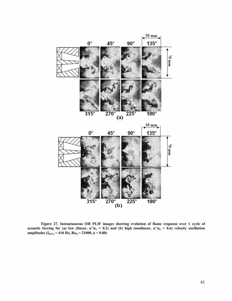
Figure 27. Instantaneous OH PLIF images showing evolution of flame response over 1 cycle of acoustic forcing for (a) low (linear, u’/uo = 0.2) and (b) high (nonlinear, u’/uo = 0.6) velocity oscillation amplitudes (fdrive = 410 Hz, ReD = 21000, φ = 0.80)
41
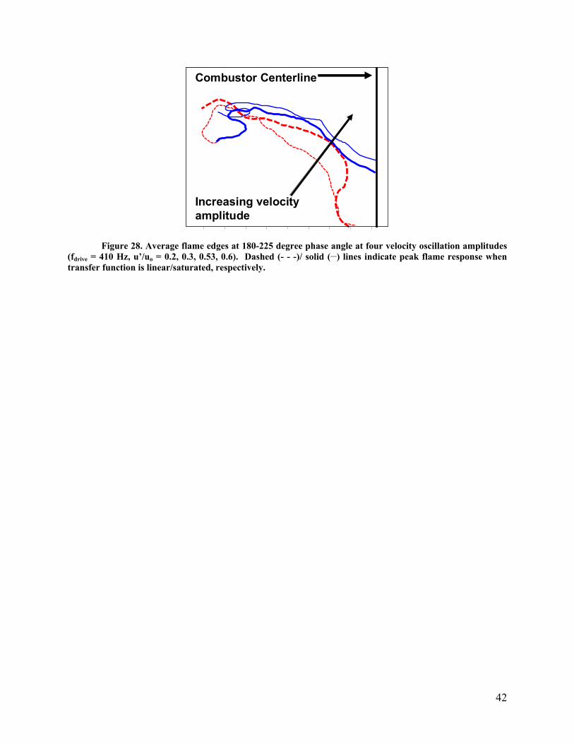
Combustor Centerline
Increasing velocity amplitude
Combustor Centerline
Increasing velocity amplitude
Figure 28. Average flame edges at 180-225 degree phase angle at four velocity oscillation amplitudes (fdrive = 410 Hz, u’/uo = 0.2, 0.3, 0.53, 0.6). Dashed (- - -)/ solid (__) lines indicate peak flame response when transfer function is linear/saturated, respectively.
42
7. THEORETICAL NONLINEAR FLAME RESPONSE
CHARACTERISTICS
This paper describes the dynamics of premixed flames responding to harmonic velocity disturbances.
Results are derived from analytical and computational solutions of the nonlinear G-equation and used to interpret a
number of experimental observations. It is shown that the linear and nonlinear characteristics of the flame dynamics
are controlled by the superposition of two sources of flame disturbances: those originating at the flame anchoring
point due to boundary conditions and from flow non-uniformities along the flame. These disturbances do not
necessarily propagate along the flame at the same speed. Consequently, they may either constructively or
destructively superpose with each other, so that the overall linear flame response depends upon two Strouhal
numbers, St2 and Stc, related to the amount of time taken for a flow (Stc) and flame front (St2) disturbance to
propagate the flame length, normalized by the acoustic period. Unsteady stretch effects, responsible for the
reduction in the flame front wrinkle size in the flow direction (referred to as “filtering” by Bouehla & Baillot25,
become significant when σ*St2~O(1), where σ* is a non-dimensionalized Markstein length. The nonlinear flame
response is driven by flame propagation normal to itself (“kinematic restoration”), which smoothens out the
wrinkles induced by the forcing. Because the overall flame response is a superposition of the two flame disturbance
contributions, the flame’s nonlinear response can exhibit two qualitatively different behaviors. For parameter values
where these disturbances constructively interfere, the nonlinear flame transfer function gain saturates and is,
therefore, always less than its linear value. When the flame disturbances destructively interfere, the nonlinear
transfer function may actually exceed its linear value before saturating. This result explains Durox et al’s27
experimentally observed variation of the nonlinear flame response with frequency. One interesting prediction of this
analysis concerns the impact of flow forcing on average flame length. We show that in most cases, the flame length
decreases with increasing perturbation amplitude, as has been experimentally observed by Bourehla & Baillot25 and
Durox et al40. However, the analysis also predicts that the flame can lengthen under certain conditions, a result that
has apparently not yet been experimentally observed.
This paper describes an analysis of the linear and nonlinear dynamics of laminar premixed flames
responding to harmonic velocity disturbances. The key objective of this work is to predict the heat release response
of the flame, and to isolate the key non-dimensional parameters which characterize these interactions. While this
problem is of great interest from a fundamental standpoint, it is also motivated by pressing practical problems. This
paper’s focus on premixed flames is motivated by the fact that low emissions combustion systems for land-based gas
turbines, future aircraft engines, industrial heaters and boilers rely on a premixed or partially premixed combustion
process. Furthermore, its focus upon harmonically oscillating flow disturbances stems from the fact that these
combustion systems are exceptionally prone to combustion instabilities3,8, 41-44 which generally occur when the
unsteady combustion process couples with the natural acoustic modes of the combustion chamber, resulting in self-
excited oscillations. These oscillations are destructive to hardware and adversely affect performance and emissions.
43
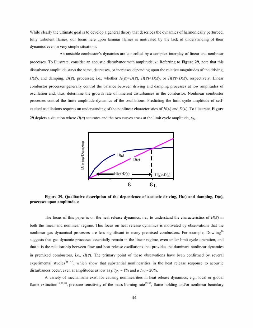
While clearly the ultimate goal is to develop a general theory that describes the dynamics of harmonically perturbed,
fully turbulent flames, our focus here upon laminar flames is motivated by the lack of understanding of their
dynamics even in very simple situations.
An unstable combustor’s dynamics are controlled by a complex interplay of linear and nonlinear
processes. To illustrate, consider an acoustic disturbance with amplitude, ε. Referring to Figure 29, note that this
disturbance amplitude stays the same, decreases, or increases depending upon the relative magnitudes of the driving,
H(ε), and damping, D(ε), processes; i.e., whether H(ε)=D(ε), H(ε)<D(ε), or H(ε)>D(ε), respectively. Linear
combustor processes generally control the balance between driving and damping processes at low amplitudes of
oscillation and, thus, determine the growth rate of inherent disturbances in the combustor. Nonlinear combustor
processes control the finite amplitude dynamics of the oscillations. Predicting the limit cycle amplitude of self-
excited oscillations requires an understanding of the nonlinear characteristics of H(ε) and D(ε). To illustrate, Figure
29 depicts a situation where H(ε) saturates and the two curves cross at the limit cycle amplitude, εLC.
ε
Driv
ing/
Dam
ping
D(ε)H(ε)
H(ε)>D(ε) H(ε)<D(ε)
εL
Figure 29. Qualitative description of the dependence of acoustic driving, H(ε) and damping, D(ε), processes upon amplitude, ε
The focus of this paper is on the heat release dynamics, i.e., to understand the characteristics of H(ε) in
both the linear and nonlinear regime. This focus on heat release dynamics is motivated by observations that the
nonlinear gas dynamical processes are less significant in many premixed combustors. For example, Dowling16
suggests that gas dynamic processes essentially remain in the linear regime, even under limit cycle operation, and
that it is the relationship between flow and heat release oscillations that provides the dominant nonlinear dynamics
in premixed combustors, i.e., H(ε). The primary point of these observations have been confirmed by several
experimental studies 45 - 47 , which show that substantial nonlinearities in the heat release response to acoustic
disturbances occur, even at amplitudes as low as p’/po ~ 1% and u’/uo ~ 20%.
A variety of mechanisms exist for causing nonlinearities in heat release dynamics; e.g., local or global
flame extinction16,19,48, pressure sensitivity of the mass burning rate49-52, flame holding and/or nonlinear boundary
44
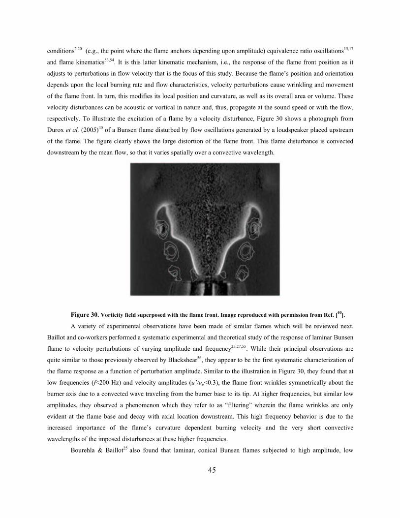
conditions2,20 (e.g., the point where the flame anchors depending upon amplitude) equivalence ratio oscillations15,17
and flame kinematics53,54. It is this latter kinematic mechanism, i.e., the response of the flame front position as it
adjusts to perturbations in flow velocity that is the focus of this study. Because the flame’s position and orientation
depends upon the local burning rate and flow characteristics, velocity perturbations cause wrinkling and movement
of the flame front. In turn, this modifies its local position and curvature, as well as its overall area or volume. These
velocity disturbances can be acoustic or vortical in nature and, thus, propagate at the sound speed or with the flow,
respectively. To illustrate the excitation of a flame by a velocity disturbance, Figure 30 shows a photograph from
Durox et al. (2005)40 of a Bunsen flame disturbed by flow oscillations generated by a loudspeaker placed upstream
of the flame. The figure clearly shows the large distortion of the flame front. This flame disturbance is convected
downstream by the mean flow, so that it varies spatially over a convective wavelength.
Figure 30. Vorticity field superposed with the flame front. Image reproduced with permission from Ref. [40].
A variety of experimental observations have been made of similar flames which will be reviewed next.
Baillot and co-workers performed a systematic experimental and theoretical study of the response of laminar Bunsen
flame to velocity perturbations of varying amplitude and frequency25,27,55. While their principal observations are
quite similar to those previously observed by Blackshear56, they appear to be the first systematic characterization of
the flame response as a function of perturbation amplitude. Similar to the illustration in Figure 30, they found that at
low frequencies (f<200 Hz) and velocity amplitudes (u’/uo<0.3), the flame front wrinkles symmetrically about the
burner axis due to a convected wave traveling from the burner base to its tip. At higher frequencies, but similar low
amplitudes, they observed a phenomenon which they refer to as “filtering” wherein the flame wrinkles are only
evident at the flame base and decay with axial location downstream. This high frequency behavior is due to the
increased importance of the flame’s curvature dependent burning velocity and the very short convective
wavelengths of the imposed disturbances at these higher frequencies.
Bourehla & Baillot25 also found that laminar, conical Bunsen flames subjected to high amplitude, low
45
frequency velocity perturbations exhibited a variety of transient flame holding behavior, such as flashback,
asymmetric blowoff, unsteady lifting and re-anchoring of the flame. In addition, they note that its response is
asymmetric and extremely disordered. However, at high frequencies and forcing amplitudes, the flame remains
firmly attached, but its overall shape dramatically changes. They found that the flame becomes “collapsed” with a
rounded off tip region, and for sufficiently high forcing intensities (u’/uo>1), the flame’s mean shape becomes
hemispherical25. Baillot et al.55 also reported a theoretical study, where they solved the G-equation and showed good
agreement between predicted and measured flame shapes, even at larger amplitudes of forcing where the flame front
becomes strongly cusped. The so-called G-equation is a front tracking equation for the flame position, given by:
LG u G S G 0t
∂+ ∇ − ∇ =
∂rg (1)
where G(x,t)=0 is an implicit expression defining the instantaneous flame position, ur is the velocity field
and SL is the laminar burning velocity.
Recent work complements the studies of Baillot and co-workers discussed above, by quantifying the global
heat release response, Q’, of the flame8,32,40. These workers obtained high speed images and transfer functions,
(Q’/Qo)/(u’/uo), of acoustically forced Bunsen and inverted wedge flames. Significantly, they showed that most of
the key flame response characteristics could be quantitatively predicted by assuming that the flame’s heat release
was directly proportional to its instantaneous area. The flame area was calculated using the G-equation, where
measured velocity fields were used as inputs.
Solution of the G-equation is a key analytical approach used in this paper, as well as the above cited
studies, for quantitative analysis of this problem. This approach for treating unsteady flame problems was apparently
first introduced by Markstein57 and, in the context of acoustically forced flames, by Marble & Candel58. It has
subsequently been extensively developed59 and is used in a variety of flame dynamic studies. The key assumption
behind its application is the separation of acoustic/hydrodynamic scales of the flow field, and the flame thickness.
Given the disparity between flame and acoustic length scales, the flame front essentially appears as a discontinuity
to the flow. As such, the fluid dynamics of the flows up and downstream of the flame can often be treated separately
from that of the flame structure. However, we should emphasize that there is not necessarily a corresponding
disparity in time scales; e.g. forming a flame response time scale, τM, from the ratio of the laminar flame thickness
and flame speed leads to values of τM~0.002 - .07 s for methane/air flames. These are of similar magnitude of
perturbations with frequencies between 20-500 Hz. Thus, the interior flame structure and, consequently, quantities
such as the flame speed, do not respond in a quasi-steady manner to flow perturbations.
Because of the mutual interaction between the flame position and the flow field, free boundary problems
such as this are extremely difficult to handle analytically. Initial studies used an integral technique58,60-63 to make it
analytically tractable. Further progress has been made in more recent studies7,8,53,60,which circumvented the
analytical difficulties encountered in the fully coupled flame-flow problem by neglecting the coupling of flow
perturbations across the flame, as will also be done in this study. As such, they calculated the response of the flame
from an imposed velocity disturbance of given amplitude and phase upstream of the flame. In essence, this
46
approximation neglects the density change across the flame front. Nonetheless, the substantially reduced complexity
of the approach facilitates a much more transparent analysis; moreover, their results give excellent agreement with
experiments in many instances. We will discuss the conditions under which this approximation is appropriate, and
not appropriate, at length below.
In closing, we should draw the readers attention to several additional analyses which, though not directly
aimed at the acoustic flame interaction problem, did analyze the kinematics of a nominally flat flame front in an
unsteady and/or periodic, prescribed, flow field; e.g., see Refs. [64-67].
The key contribution of the present work is to provide a systematic treatment of linear and nonlinear flame
dynamics – including unsteady stretch effects - in response to harmonically oscillating flow disturbances. The rest of
the paper is organized in the following manner: Section 0 describes the key processes impacting the flame dynamics
and the disturbance field. In particular, the principle assumptions of the analysis are identified and the phenomena
which can and cannot be captured by the analysis are discussed. Section 0 presents the modeling approach and
analysis procedure. Section 0 presents results that quantify the effects of flame geometry, disturbance field
characteristics, perturbation frequency and stretch sensitivity upon the flames linear (Section 0) and nonlinear
(Section 0) characteristics. The response of the flame at the perturbation frequency and its harmonics are discussed
as well as changes in the mean flame length.
Basic Considerations
Flame Dynamics
The basic problem of interest is this: Given a disturbance velocity field, ( ),t′ ru x , determine the response of
the flame position, ( )x,tζr
, and in particular, the total heat release rate of the flame. The global heat release rate of
the flame is given by:
1 L R FLs
Q( t ) S h dAρ ∆= ∫ (2)
where the integral is performed over the flame surface, AFL, and ∆hR is the heat release per unit mass of
reactant. Equation (2) shows the three fundamentally different ways of generating heat release disturbances in a
premixed flame: fluctuations in mass burning rate (ρ1SL), heat of reaction, or flame area. As noted by Clanet et al.68,
they can be classified based upon either their modification of the local internal structure of the flame (such as the
local burning rate) or its global geometry (such as its area).
As we are focused upon the flame response to flow perturbations, we assume constant ∆hR and mixture
density, ρ1; analysis of the effects of these perturbations are given in Refs. [49,69]. Of course, if the flow
perturbation is acoustic in origin, a density disturbance will accompany the velocity fluctuation. However, their
relative impacts differ greatly, on the order of the flame speed Mach number. As such, our subsequent calculations
focus upon the quantity:
47
L FL FL
L FL FL
S dA AQQ S dA A
′ ′′ ∫= +∫
(3)
Flame speed perturbations are generated by the oscillating stretch rate, proportional to ∇2G, and are
discussed in Section 0. Flame area fluctuations are directly related to perturbations in the flame position through the
relation:
( )FL oA ( t ) G G G dSδ= − ∇∫ (4)
where Go denotes the flame surface. This equation shows that the quantity of interest is not G itself, but its
gradient ∇G - a very important observation. Another key observation is that only the velocity component normal to
the flame, nu n u⋅ =r r
, a scalar quantity, impacts the flame dynamics. This can be seen by rewriting Eq. (1) as:
( )n LG u S G 0t
∂+ − ∇ =
∂ (5)
This necessarily implies that the full three dimensional details of the velocity field are not significant; it is
only the component that is normal to the flame. As such a detailed specification of the velocity field is not necessary
for an understanding of the flame dynamics and, furthermore, a variety of different velocity fields can give an
essentially identical flame response. This is the reason why we assume a relatively simple form of the disturbance
velocity field, as will be detailed in Sec. 0. However, for large amplitude oscillations, this point must be conditioned
with the fact that the flame normal exhibits large fluctuations, so the relative contribution of each vector component
of the velocity field varies throughout the cycle.
Several general comments can be made regarding the dynamics of the flame position gradient, which is
directly related to its surface area through Eq (4); these will provide a great deal of insight into the flame dynamics.
From a mathematical point of view, the linear solution to the equation for flame surface area can be decomposed
into two canonical components: the homogeneous solution and the particular solution. The linearized version of Eq.
(1) can be written in a coordinate system aligned normal to the mean flame position as (see Figure 31)
(oU U Xt Xξ ξ∂ ∂ ′+ =
∂ ∂),t
)
(6)
where X denotes the coordinate along the mean flame position, Uo is the mean velocity component along
the X axis and ( X ,tξ is the perturbed flame position normal to this coordinate. The dynamics of / Xξ∂ , which is
directly related to that of the flame area itself, is described by the following solution
∂
*:
* In Eq (7), after evaluating the velocity gradient ∂U’/∂X, the integration has to be performed with respect to
dx’after replacing the variable X by x’ and t by t-(X-x’)/Uo
48
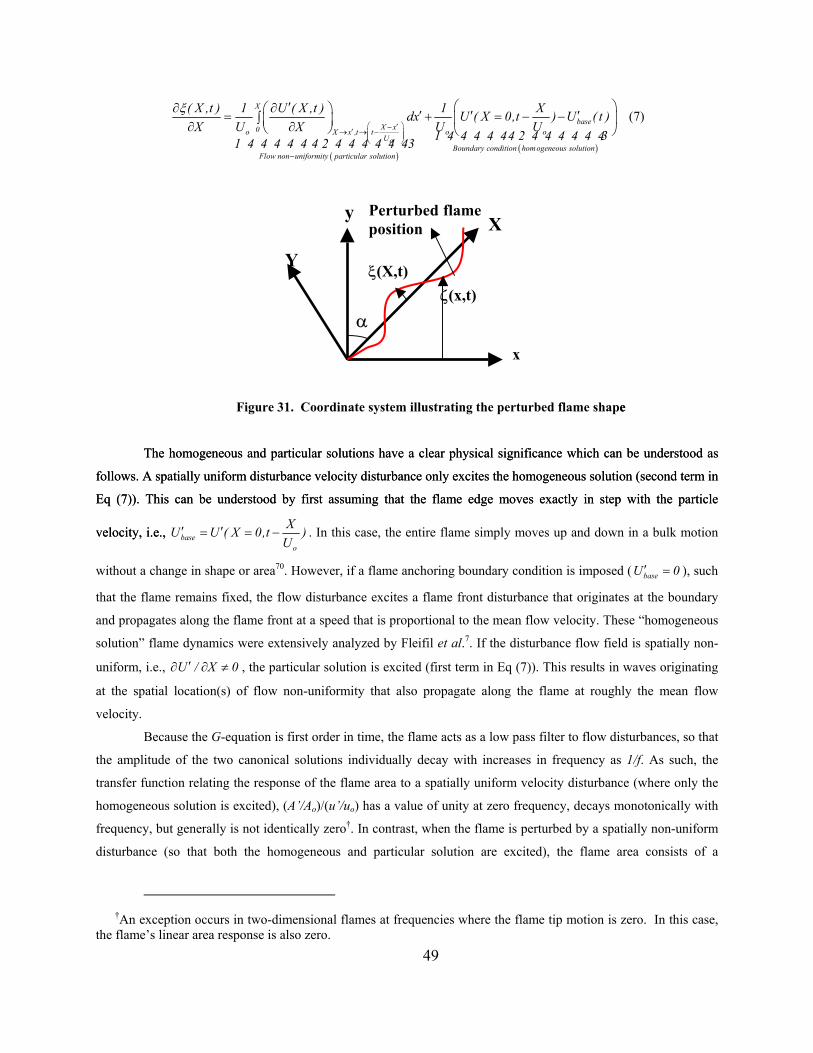
( )( )
X
baseX x0o oX x ,t tUo
Boundary condition hom ogeneous solutionFlow non uniformity particular solution
( X ,t ) 1 U ( X ,t ) 1 Xdx U ( X 0,t ) U ( t )X U X U U
ξ ′−′→ → −
−
′∂ ∂ ′ ′ ′= + =∫ ∂ ∂ 1 4 4 4 4 44 2 4 4 4 4 4 431 4 4 4 4 4 4 2 4 4 4 4 4 43o
− − (7)
Y
X
ξ(X,t) ζ(x,t)
Perturbed flameposition
y
α
x
Figure 31. Coordinate system illustrating the perturbed flame shape e
The homogeneous and particular solutions have a clear physical significance which can be understood as
follows. A spatially uniform disturbance velocity disturbance only excites the homogeneous solution (second term in
Eq (7)). This can be understood by first assuming that the flame edge moves exactly in step with the particle
velocity, i.e.,
The homogeneous and particular solutions have a clear physical significance which can be understood as
follows. A spatially uniform disturbance velocity disturbance only excites the homogeneous solution (second term in
Eq (7)). This can be understood by first assuming that the flame edge moves exactly in step with the particle
velocity, i.e., baseo
XU U . In this case, the entire flame simply moves up and down in a bulk motion
without a change in shape or area
( X 0,tU
′ ′= = − )
070. However, if a flame anchoring boundary condition is imposed (Ubase′ = ), such
that the flame remains fixed, the flow disturbance excites a flame front disturbance that originates at the boundary
and propagates along the flame front at a speed that is proportional to the mean flow velocity. These “homogeneous
solution” flame dynamics were extensively analyzed by Fleifil et al.7. If the disturbance flow field is spatially non-
uniform, i.e., ∂ ∂ , the particular solution is excited (first term in Eq (7)). This results in waves originating
at the spatial location(s) of flow non-uniformity that also propagate along the flame at roughly the mean flow
velocity.
U / X 0′ ≠
Because the G-equation is first order in time, the flame acts as a low pass filter to flow disturbances, so that
the amplitude of the two canonical solutions individually decay with increases in frequency as 1/f. As such, the
transfer function relating the response of the flame area to a spatially uniform velocity disturbance (where only the
homogeneous solution is excited), (A’/Ao)/(u’/uo) has a value of unity at zero frequency, decays monotonically with
frequency, but generally is not identically zero†. In contrast, when the flame is perturbed by a spatially non-uniform
disturbance (so that both the homogeneous and particular solution are excited), the flame area consists of a
†An exception occurs in two-dimensional flames at frequencies where the flame tip motion is zero. In this case,
the flame’s linear area response is also zero.
49
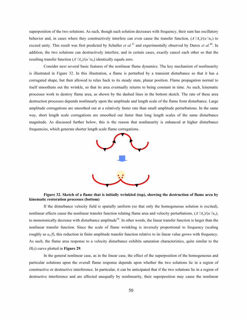
superposition of the two solutions. As such, though each solution decreases with frequency, their sum has oscillatory
behavior and, in cases where they constructively interfere can even cause the transfer function, (A’/Ao)/(u’/uo) to
exceed unity. This result was first predicted by Schuller et al.32 and experimentally observed by Durox et al.40. In
addition, the two solutions can destructively interfere, and in certain cases, exactly cancel each other so that the
resulting transfer function (A’/Ao)/(u’/uo) identically equals zero.
Consider next several basic features of the nonlinear flame dynamics. The key mechanism of nonlinearity
is illustrated in Figure 32. In this illustration, a flame is perturbed by a transient disturbance so that it has a
corrugated shape, but then allowed to relax back to its steady state, planar position. Flame propagation normal to
itself smoothens out the wrinkle, so that its area eventually returns to being constant in time. As such, kinematic
processes work to destroy flame area, as shown by the dashed lines in the bottom sketch. The rate of these area
destruction processes depends nonlinearly upon the amplitude and length scale of the flame front disturbance. Large
amplitude corrugations are smoothed out at a relatively faster rate than small amplitude perturbations. In the same
way, short length scale corrugations are smoothed out faster than long length scales of the same disturbance
magnitude. As discussed further below, this is the reason that nonlinearity is enhanced at higher disturbance
frequencies, which generate shorter length scale flame corrugations.
Figure 32. Sketch of a flame that is initially wrinkled (top), showing the destruction of flame area by kinematic restoration processes (bottom)
If the disturbance velocity field is spatially uniform (so that only the homogeneous solution is excited),
nonlinear effects cause the nonlinear transfer function relating flame area and velocity perturbations, (A’/Ao)/(u’/uo),
to monotonically decrease with disturbance amplitude54. In other words, the linear transfer function is larger than the
nonlinear transfer function. Since the scale of flame wrinkling is inversely proportional to frequency (scaling
roughly as uo/f), this reduction in finite amplitude transfer function relative to its linear value grows with frequency.
As such, the flame area response to a velocity disturbance exhibits saturation characteristics, quite similar to the
H(ε) curve plotted in Figure 29.
In the general nonlinear case, as in the linear case, the effect of the superposition of the homogeneous and
particular solutions upon the overall flame response depends upon whether the two solutions lie in a region of
constructive or destructive interference. In particular, it can be anticipated that if the two solutions lie in a region of
destructive interference and are affected unequally by nonlinearity, their superposition may cause the nonlinear
50
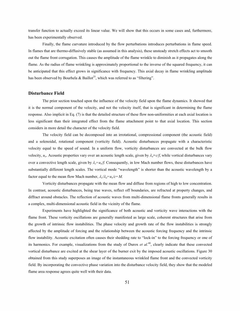
transfer function to actually exceed its linear value. We will show that this occurs in some cases and, furthermore,
has been experimentally observed.
Finally, the flame curvature introduced by the flow perturbations introduces perturbations in flame speed.
In flames that are thermo-diffusively stable (as assumed in this analysis), these unsteady stretch effects act to smooth
out the flame front corrugation. This causes the amplitude of the flame wrinkle to diminish as it propagates along the
flame. As the radius of flame wrinkling is approximately proportional to the inverse of the squared frequency, it can
be anticipated that this effect grows in significance with frequency. This axial decay in flame wrinkling amplitude
has been observed by Bourhela & Baillot25, which was referred to as “filtering”.
Disturbance Field The prior section touched upon the influence of the velocity field upon the flame dynamics. It showed that
it is the normal component of the velocity, and not the velocity itself, that is significant in determining the flame
response. Also implicit in Eq. (7) is that the detailed structure of these flow non-uniformities at each axial location is
less significant than their integrated effect from the flame attachment point to that axial location. This section
considers in more detail the character of the velocity field.
The velocity field can be decomposed into an irrotational, compressional component (the acoustic field)
and a solenoidal, rotational component (vorticity field). Acoustic disturbances propagate with a characteristic
velocity equal to the speed of sound. In a uniform flow, vorticity disturbances are convected at the bulk flow
velocity, uo. Acoustic properties vary over an acoustic length scale, given by λa=c/f, while vortical disturbances vary
over a convective length scale, given by λc=uo/f. Consequently, in low Mach number flows, these disturbances have
substantially different length scales. The vortical mode “wavelength” is shorter than the acoustic wavelength by a
factor equal to the mean flow Mach number, λc/λa=uo/c=M.
Vorticity disturbances propagate with the mean flow and diffuse from regions of high to low concentration.
In contrast, acoustic disturbances, being true waves, reflect off boundaries, are refracted at property changes, and
diffract around obstacles. The reflection of acoustic waves from multi-dimensional flame fronts generally results in
a complex, multi-dimensional acoustic field in the vicinity of the flame.
Experiments have highlighted the significance of both acoustic and vorticity wave interactions with the
flame front. These vorticity oscillations are generally manifested as large scale, coherent structures that arise from
the growth of intrinsic flow instabilities. The phase velocity and growth rate of the flow instabilities is strongly
affected by the amplitude of forcing and the relationship between the acoustic forcing frequency and the intrinsic
flow instability. Acoustic excitation often causes their shedding rate to “lock-in” to the forcing frequency or one of
its harmonics. For example, visualizations from the study of Durox et al.40, clearly indicate that these convected
vortical disturbance are excited at the shear layer of the burner exit by the imposed acoustic oscillations. Figure 30
obtained from this study superposes an image of the instantaneous wrinkled flame front and the convected vorticity
field. By incorporating the convective phase variation into the disturbance velocity field, they show that the modeled
flame area response agrees quite well with their data.
51
The characteristics of the instability waves that grow and merge to form these large scale structures are a
function of the specific characteristics of the burner exit shear layer, such as co-flow velocity, and specifically upon
the receptivity of this shear layer to external disturbances. In addition, the phase speed of the convected vortical
instability waves are not equal to the flow velocity, but vary with frequency and shear layer characteristics. The
instability wave growth rate similarly varies with frequency and the shear layer characteristics. To illustrate, Figure
33 plots Michalke’s73 theoretical curves of the dependence of the phase speed, uc, of shear layer instability waves in
a jet flow upon Strouhal number, Sθ=fθ/uo, for several values of the momentum thickness, θ, to jet radius, R, ratio,
R/θ. The figure shows that, for all R/θ values, the ratio of uc/uo equals unity and 0.5 for low and high Strouhal
numbers. For thin boundary layers, e.g., R/θ =100, the phase velocity actually exceeds the maximum axial flow
velocity in a certain Sθ range. This ultra-fast phase velocity prediction has been experimentally verified by Bechert
& Pfizenmaier71 and may explain a similar measurement in a Bunsen flame by Ferguson et al.72. The dispersive
character of the instability wave convection velocity has been confirmed by a variety of measurements in
acoustically forced flames. For example, Baillot et al.53 measured uc/uo values of 1.13 and 1.02 at 35 and 70 Hz,
respectively, on a conical Bunsen flame. Durox et al.40 measured uc/uo =0.5 values at 150 Hz in an axisymmetric
wedge flame.
Figure 33. Dependence of shear wave convection velocity and growth rate in a jet flow upon Strouhal number and ratio of jet radius to momentum thickness. Figure reproduced from Michalke73 (1971).
In general, the disturbance field may have both acoustic and vortical components, whose relative
magnitude depends strongly upon the vortex shedding dynamics at the burner shear layer. For example, Ferguson et
al.72 found that the disturbance field transitioned from a convected character to one with an acoustic character at
“low” and “high” frequencies, respectively. This behavior may be due to the corresponding dependence of vorticity
wave growth rate upon frequency. These points show that the character of the disturbance field can vary
significantly between its relative acoustic and vortical components, as well as their spatial structure (such as phase
speed) – these characteristics will change with experimental configuration, frequency, and amplitude of
52
perturbation. This point is a key motivator for our development of a general theory for arbitrary phase speed velocity
disturbances.
The amplitude dependence of the disturbance field characteristics should be noted. Even in the absence of
convected vorticity waves, the impact of the fluctuating flame position upon the acoustic field should cause the
acoustic disturbance field to have a “convected” character. This is due to the fact that the flame response to the
acoustic field and the acoustic field disturbing the flame are coupled. For large amplitude disturbances, the flame
develops large corrugations, such as can be seen in Figure 30, that convect with a phase speed proportional to the
axial flow velocity. These convecting flame wrinkles impact the character of the interior acoustic field. It can be
anticipated that this mechanism causes the acoustic field structure to revert from being nearly uniform (assuming a
compact flame) to having some convected charactereristics at low and high amplitude disturbances, respectively.
This issue requires further clarification, as the effects of amplitude and frequency on the acoustic field structure have
not been measured or calculated in the large amplitude case.
In this analysis, we prescribe, rather than solve for, the velocity field as done in most recent
studies of the problem. In general, it should be emphasized that the thermal expansion of gases at the flame front
causes the flame to influence the velocity field upstream of it; this coupling is responsible for the Darrius-Landau
flame instability. We next turn attention to the very important issue of the manner in which these mutual interactions
impact the results, the conditions under which the present analysis is appropriate, and the conditions where
additional physics qualitatively influences the flame dynamics.
First it should be noted that imposing the velocity field is a rigorously valid approximation in the limit of
low dilatation flames; i.e., in the limit where Tb/Tu→1. This is also the limit considered by other authors for studies
of the thermal-diffusive instability and is the basis of the Sivashinsky-Kuramoto equation74,75. Besides being of
academic interest in allowing one to analytically handle the problem, this is actually a useful limit for many practical
devices. It is often pointed out in the combustion literature that practical flames have temperature ratios on the order
of 6-10. This is true for flame’s consuming reactants at room temperature but not, however, for the conditions
encountered in most practical devices. Due to the need for high efficiencies (e.g., devices utilizing regenerative
heating or high compression ratios such as industrial boilers or gas turbines) or because the devices are using
vitiated air (duct burners or jet engine augmentors), unburned gas temperatures are substantially higher.
Correspondingly, the requirement for low NOx emissions implies lower burned gas temperatures. As such, typical
temperature ratios for practical premixed combustion devices are in the range of 2-3, and even as low as 1.5 in
certain industrial applications with large amounts of regenerative pre-heating.
Clearly, however, as Tb/Tu deviates from unity, there will be an impact upon the approach flow
characteristics. It can readily be shown that the impact of the flame on the acoustic field scales as (Tb/Tu)1/2, which is
the ratio of the gas impedances across the flame. Based upon the discussion in the prior section it can be anticipated
that, at least for low amplitude perturbations, the alteration of the local acoustic field by the flame does not introduce
qualitative changes into the flame dynamics, although it may certainly exert quantitative impacts that increase as
(Tb/Tu)1/2. This assertion has been previously confirmed by Lee & Lieuwen70, who computationally determined the
53

flame’s acoustic nearfield for various Tb/Tu values, determined the flame area response, and compared the results to
the constant density analyses of Fleifil et al.7 and Ducruix et al.8.
Similarly, it is known that the effect of a stable flame on the vortical approach flow velocity scales
approximately as Tb/Tu76 As in the acoustic case, there is clearly also a frequency-wavenumber dependence, as well
as an inverse dependency upon proximity to flame stability boundaries.
The qualitative similarities between fully coupled flame dynamics and that determined using an imposed
velocity field break down when both Tb/Tu and perturbation velocity amplitudes are large; i.e., new dynamics appear
that cannot be captured with this analysis. This is due to the appearance of a parametric flame instability35,36,77,
manifested by cellular structures that oscillate at half the period of the disturbance. This parametric acoustic
instability is due to the periodic acceleration of the flame front by the unsteady velocity field, which separates two
regions of differing densities. With increased amplitudes, these organized cellular structures break down into a
highly disordered, turbulent front. The regimes in Tb/Tu vs u’/SL space where this instability occurs can be
determined from from Eq. (1) in Bychkov’s analysis for a given dimensionless frequency, defined as f
LSw
ωδ=
where ω is the forcing frequency and δf is the flame thickness35. The results are plotted in Figure 34. This graph
illustrates the regions (above the curve) where application of a prescribed velocity theory is inappropriate. As could
be anticipated, it shows that the range of disturbance amplitudes diminishes with increasing temperature ratio across
the flame.
Figure 34. Parametric stability limits of flat flame (unity Lewis and Prandlt number, no gravity).
As such, we conclude that the qualitative linear dynamics of the flame are captured by this analysis for all
Tb/Tu values, although the quantitative accuracy of the results deteriorates as Tb/Tu increases. Calculations that
quantify these effects are given in Lee & Lieuwen70. In contrast, the nonlinear dynamics of the flame are only
correctly described by this analysis for low Tb/Tu values. This is the reason for the restriction to low heat release
flames indicated in the title of this paper.
54
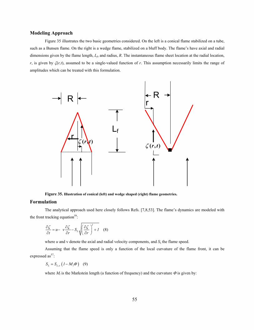
Modeling Approach Figure 35 illustrates the two basic geometries considered. On the left is a conical flame stabilized on a tube,
such as a Bunsen flame. On the right is a wedge flame, stabilized on a bluff body. The flame’s have axial and radial
dimensions given by the flame length, Lf, and radius, R. The instantaneous flame sheet location at the radial location,
r, is given by ζ(r,t), assumed to be a single-valued function of r. This assumption necessarily limits the range of
amplitudes which can be treated with this formulation.
Lf
R R
r
),( trζ),( trζ
r
Figure 35. Illustration of conical (left) and wedge shaped (right) flame geometries.
Formulation The analytical approach used here closely follows Refs. [7,8,53]. The flame’s dynamics are modeled with
the front tracking equation59:
2
Lu v S 1t r rζ ζ ζ∂ ∂ ∂ = − − + ∂ ∂ ∂
(8)
where u and v denote the axial and radial velocity components, and SL the flame speed.
Assuming that the flame speed is only a function of the local curvature of the flame front, it can be
expressed as57:
( )L L,o lS S 1 Μ Φ= − (9)
where Ml is the Markstein length (a function of frequency) and the curvature Φ is given by:
55
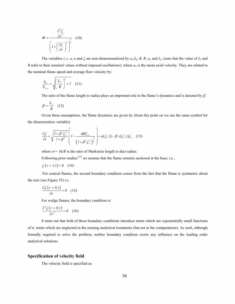
2
2
32 2
r
1r
ζ
Φ
ζ
∂∂=
∂ + ∂
(10)
The variables t, r, a, u and ζ are non-dimensionalized by uo/Lf, R, R, uo and Lf. (note that the value of Lf and
R refer to their nominal values without imposed oscillations), where uo is the mean axial velocity. They are related to
the nominal flame speed and average flow velocity by:
2fo
L,o
Lu1
S R
= +
(11)
The ratio of the flame length to radius plays an important role in the flame’s dynamics and is denoted by β.
fLR
β = (12)
Given these assumptions, the flame dynamics are given by (from this point on we use the same symbol for
the dimensionless variable):
( )( ) ( )
2 2r rr
r2 32 2 2
r
11 u ,t v
t 11
β ζ σβζζ ,tζ β ζ ζβ
β ζ
+∂
+ − = − ∂ + +
(13)
where σ = Ml/R is the ratio of Markstein length to duct radius.
Following prior studies7,53 we assume that the flame remains anchored at the base; i.e.,
( )r 1,t 0ζ = = (14)
For conical flames, the second boundary condition comes from the fact that the flame is symmetric about
the axis (see Figure 35) i.e.
( )r 0,t0
rζ∂ =
=∂
(15)
For wedge flames, the boundary condition is:
( )2
2
r 0,t0
rζ∂ =
=∂
(16)
It turns out that both of these boundary conditions introduce terms which are exponentially small functions
of σ, terms which are neglected in the ensuing analytical treatments (but not in the computations). As such, although
formally required to solve the problem, neither boundary condition exerts any influence on the leading order
analytical solutions.
Specification of velocity field The velocity field is specified as:
56
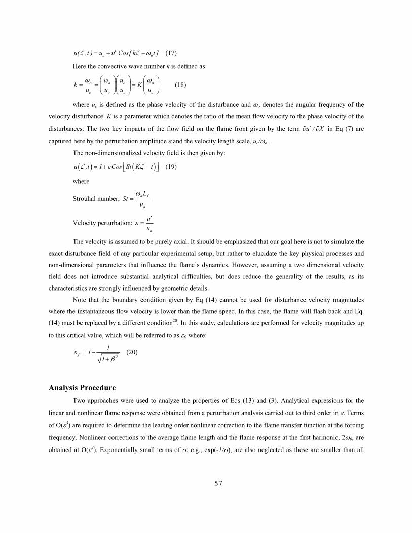
o ou( ,t ) u u Cos[ k t ]ζ ζ ω′= + − (17)
Here the convective wave number k is defined as:
o o o
c o c o
uk K
u u u uoω ω ω
= = =
(18)
where uc is defined as the phase velocity of the disturbance and ωo denotes the angular frequency of the
velocity disturbance. K is a parameter which denotes the ratio of the mean flow velocity to the phase velocity of the
disturbances. The two key impacts of the flow field on the flame front given by the term ∂ in Eq (7) are
captured here by the perturbation amplitude ε and the velocity length scale, u
u / X′ ∂
c/ωo.
The non-dimensionalized velocity field is then given by:
( ) ( )u ,t 1 Cos St K tζ ε ζ = + − (19)
where
Strouhal number, o f
o
Lu
ω=St
Velocity perturbation: o
uu
ε′
=
The velocity is assumed to be purely axial. It should be emphasized that our goal here is not to simulate the
exact disturbance field of any particular experimental setup, but rather to elucidate the key physical processes and
non-dimensional parameters that influence the flame’s dynamics. However, assuming a two dimensional velocity
field does not introduce substantial analytical difficulties, but does reduce the generality of the results, as its
characteristics are strongly influenced by geometric details.
Note that the boundary condition given by Eq (14) cannot be used for disturbance velocity magnitudes
where the instantaneous flow velocity is lower than the flame speed. In this case, the flame will flash back and Eq.
(14) must be replaced by a different condition20. In this study, calculations are performed for velocity magnitudes up
to this critical value, which will be referred to as εf, where:
f 2
111
εβ
= −+
(20)
Analysis Procedure Two approaches were used to analyze the properties of Eqs (13) and (3). Analytical expressions for the
linear and nonlinear flame response were obtained from a perturbation analysis carried out to third order in ε. Terms
of O(ε3) are required to determine the leading order nonlinear correction to the flame transfer function at the forcing
frequency. Nonlinear corrections to the average flame length and the flame response at the first harmonic, 2ω0, are
obtained at O(ε2). Exponentially small terms of σ; e.g., exp(-1/σ), are also neglected as these are smaller than all
57
powers of σ, i.e., 1
n
0L ime σσ
σ−
→< , where n is any integer.
For the fully nonlinear case, Eq.(13) is solved numerically. A robust numerical scheme is necessary which
can accurately capture the formation of sharp gradients and cusps in the distorted flame front. Spatial derivatives are
discretized using a Weighted Essentially Non-Oscillatory (WENO) scheme designed specifically for Hamilton-
Jacobi equations79. This scheme is uniformly fifth order accurate in regions wherein the spatial gradients are smooth
and third order accurate in discontinuous regions. Derivatives at the boundary nodes are calculated using fifth order
accurate upwind-differencing schemes so that only the nodes inside the computational domain are utilized. A Total
Variation Diminishing (TVD) Runge-Kutta scheme80, up to third order accurate, is used for time integration. The
flame front perturbation is tracked and the corresponding change in the flame surface area is calculated as a function
of time for a given upstream flow velocity perturbation. The transfer function relating the flame area to the
convective velocity perturbation is then evaluated. The flame response at a given frequency was determined from
the Fourier transform of the flame area at that frequency.
Results and Discussion
Linear Flame Dynamics In this section, we derive expressions for the flame area-velocity transfer function that generalize the result
of Schuller et al.32, by determining the response of a flame to a disturbance with an arbitrary phase velocity and
curvature dependent flame speed.
Flame shape The flame position is expanded as53:
( ) ( ) ( ) ( ) ( ) ( )2 3o 1 2 3r ,t r r ,t r ,t r ,t O 4ζ ζ ζ ε ζ ε ζ ε ε= + + + + (21)
The evolution equation for ζ1(r,t) is computed here and the ζ2(r,t), ζ3(r,t) terms are computed in Section 0.
The mean flame shape in the absence of perturbations is given by
1
o ( r ) 1 r O e σζ−
= − +
(22)
Stretch effects at the flame tip provide an exponentially small correction to ζo(r). An exact expression for
ζo(r) is given in Appendix A. Substituting Eqs (21) and (22) into Eq (13), the evolution equation for ζ1 is:
( ){ }
221 1 1
2 3 / 2 22Cos St K(1 r ) t 0
t r1 r1
ζ ζ ζβ σββ β
∂ ∂ ∂ − − − − − ∂ ∂+ ∂+
= (23)
The solution of Eq. (23), given the boundary condition in Eq. (14) and Eq. (15) (for conical flames) or Eq.
(16) (for wedge flames) (only terms of O(σ*) are shown below for brevity, full solutions are in Appendix B) is
58
( )
}{ }{
1 1,BC 1,Flow
2 2 2
2 2
2
2
St ( r 1 t ) St ( r 1 t )( r 1) St Sin Cos
( 1) St ( 1)
Cos St K( r 1) t Sin St K( r 1) t
( 1) St( 1)
ζ ζ ζ
α αα σ σ ηα α
α η α η
σ η
ηα η
∗ ∗
∗
= +
− + − + + − = − − −
− + − + + − −−
(24)
where 2
2 1βα
β=
+ (25)
2
(1 )
1
σ σ ασαβ β
−∗ = =
+ (26)
Kη α= (27)
This equation explicitly decomposes the solution into contributions from boundary conditions and flow
forcing non-uniformities. Note that this expression is valid for both conical and wedge flames (i.e. the second
boundary condition is satisfied by the exponentially small terms which have been neglected in the above
expressions.). The flame front position is controlled by the superposition of the flame disturbances created at each
point due to flow non-uniformity and disturbances originating from the flame base that are convected along the
flame front. The stretch contribution is controlled by the parameter σ* and becomes prominent when σ*St ~O(1).
The limit where 1η → (corresponding to instances where the two disturbances propagate along the flame
at the same speed), requires special care and is given by:
( )( )2 2
1 31
( r 1) ( r 1)2 St ( r 1) Cos[ St t ] 4 St Sin[ St t ]Lim r 1
2η
α σ σ αα αζ
α
∗ ∗
→
− − + − + + + = −
(28)
Note that for this case stretch effects have a stronger impact at high Strouhal numbers (σ*St2 ~O(1)).
In order to illustrate the effect of stretch on the flame shape, the deviation of the flame front from its
average position is shown in Figure 36. The point X=0 in Figure 36corresponds to the point of attachment at the
flame base. In the absence of stretch (σ*=0), it is well known that the flame front exhibits sinusoidal wrinkling with
a constant amplitude60. However, in the presence of stretch, the amplitude of the flame front perturbation decays
continuously from the flame base to the tip, see Figure 36. This feature wherein the oscillations on the flame front
are only evident at the flame base and become strongly damped at axial locations downstream has been
experimentally observed and referred to as “filtering” by Bourhela & Baillot25. They observed this phenomenon for
a conical flame under conditions corresponding to St>38, β=2 and σ*~0.005, the same conditions simulated in the
figure. The strong damping in the flame front oscillations away from the flame base at the same conditions is clearly
59
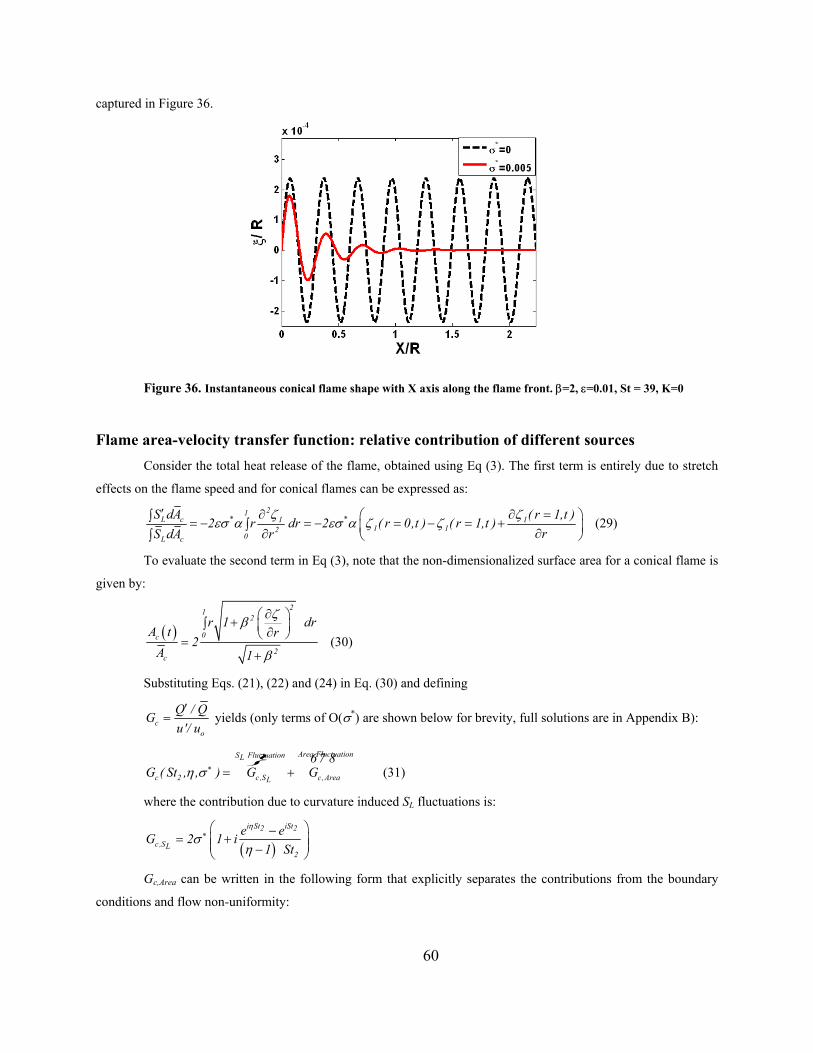
captured in Figure 36.
Figure 36. Instantaneous conical flame shape with X axis along the flame front. β=2, ε=0.01, St = 39, K=0
Flame area-velocity transfer function: relative contribution of different sources Consider the total heat release of the flame, obtained using Eq (3). The first term is entirely due to stretch
effects on the flame speed and for conical flames can be expressed as: 21
* *L c 1 11 12
0L c
S dA ( r 1,t )2 r dr 2 ( r 0,t ) ( r 1,t )
rrS dAζ ζ
εσ α εσ α ζ ζ′ ∂ ∂ ∫ = − = − = − = +∫ ∂∂ ∫
= (29)
To evaluate the second term in Eq (3), note that the non-dimensionalized surface area for a conical flame is
given by:
( )21
2
0c
2c
r 1 drA t r
2A 1
ζβ
β
∂ +∫ ∂ =+
(30)
Substituting Eqs. (21), (22) and (24) in Eq. (30) and defining
co
Q / QGu'/ u
′= yields (only terms of O(σ*) are shown below for brevity, full solutions are in Appendix B):
} Area FluctuationS FluctuationL
c 2 c,S c ,AreaLG ( St , , ) G Gη σ ∗ = +
67 8(31)
where the contribution due to curvature induced SL fluctuations is:
( )i St iSt2 2
c ,SL2
e eG 2 1 i1 St
η
ση
∗ −
= + −
Gc,Area can be written in the following form that explicitly separates the contributions from the boundary
conditions and flow non-uniformity:
60
( )( )
( ) ( ) ( )
c ,Area c,Area ,BC c,Area ,Flow
iSt iSt2 22 2iSt i St i St2 2 222 2 22 2 22 22 2
Boundary Condition
G G G
i( e 1)(1 ) St e (1 )e 1 iSt 1 e i St ie i St2 2
1 St 1 St1 St 1 St
η ηη η η η η ησ σ
η η ηη η∗ ∗
= +
− − + + − +− − − + − + = + + − − −− − 1 4 4 4 4 4 4 4 4 4 4 4 44 2 4 4 4 4 4 4 4 4 4 4 4 4 43
Flow non uniformity−
1 4 4 4 4 4 4 44 2 4 4 4 4 4 4 4 43
2η
Alternatively, it can be written in a form which separates out the stretch effects:
( )( )
( )( )( ) ( )
i St i St2 2iSt i St 2 22 2 i St2
c ,Area 2 22 2
Stretch Contribution to Area Fluctuation
e 1 e ( 1)1 e e 1 eG 2 2 i11 St 1 St
ηη η η η ηησ
ηη η η∗
− + − − −− + − = + −− − 1 4 4 4 4 4 4 4 4 4 4 2 4 4 4 4 4 4 4 4 4 43
+
where
( )2
2 2
St 1StStβ
α β
+= = (32)
Following a similar procedure, the following result can be obtained for wedge flames:
212
0w
2w
(1 r ) 1 drrA ( t )
2A 1
ζβ
β
∂ − +∫ ∂ =+
(33)
}
( )
( )( )
( )
Area FluctuationS FluctuationL
w 2 w,S w,AreaL
iSt i St2 22 2
w,SL2
iSt iSt iSt2 22 2 2iSt2 2 22w,Area 2 2
2 2
B
G ( St , , ) G G
( i St )e ( i St )eG 2
1 St
i( e 1) St e (1 ) i( 1)St e1 i( i St )eG 2
1 St 1 St
η
η σ
ησ
η
η η ησ
η η
∗
∗
∗
= +
+ − += −
− + − + + −+ + = − − −
6 7 8
( ) ( )
oundary Condition
i St i St2 22 2
2 22 2
Flow non uniformity
iSt i St2 22 2
22
(1 i St )e 1 e ( i St ) i2
1 St 1 St
1 i( i St ) e (1 i St )e2
( 1)St
η η
η
η ησ η
η η η
η η ηη η
∗
−
− − + − + + − −
− + + + −= −
1 4 4 4 4 4 4 4 4 4 4 4 4 4 44 2 4 4 4 4 4 4 4 4 4 4 4 4 4 4 43
1 4 4 4 4 4 4 4 44 2 4 4 4 4 4 4 4 4 43
( )( )( ) ( ) ( )
i St i St2 22 2 i Sti St i St2 2 22 22
2 22
Stretch Contribution to Area fluctuation
e 1 e ( 1) iSt e( 1)e e2 i11 St 1
η ηη η η η η η ησηη η
∗
− + − − − − + − − − −− − 1 4 4 4 4 4 4 4 4 4 4 4 4 4 4 4 442 4 4 4 4 4 4 4 4 4 4 4 4 4 4 4 443
+
(34)
The above results reduce to those previously developed by Schuller et al.32 when σ*=0 and the phase speed
of the disturbances is equal to that of the mean flow (i.e. K=1) (note that they refer to St2 as ω* and α as Cos2α).
61
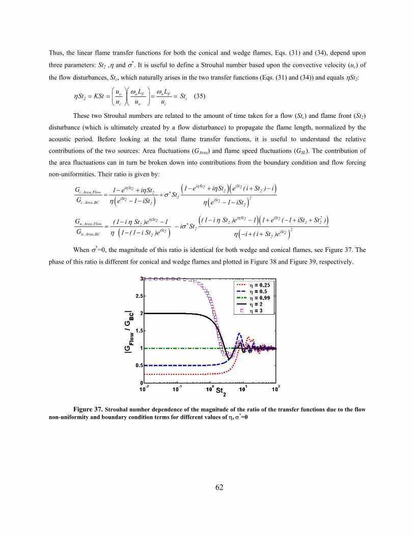
Thus, the linear flame transfer functions for both the conical and wedge flames, Eqs. (31) and (34), depend upon
three parameters: St2 ,η and σ*. It is useful to define a Strouhal number based upon the convective velocity (uc) of
the flow disturbances, Stc, which naturally arises in the two transfer functions (Eqs. (31) and (34)) and equals ηSt2:
o o F o F2 c
c o c
u L LSt KSt St
u u uω ω
η
= = = =
(35)
These two Strouhal numbers are related to the amount of time taken for a flow (Stc) and flame front (St2)
disturbance (which is ultimately created by a flow disturbance) to propagate the flame length, normalized by the
acoustic period. Before looking at the total flame transfer functions, it is useful to understand the relative
contributions of the two sources: Area fluctuations (GArea) and flame speed fluctuations (GSL). The contribution of
the area fluctuations can in turn be broken down into contributions from the boundary condition and flow forcing
non-uniformities. Their ratio is given by:
( )( )( )
( )
i St iSt2 2i St2 2 2c ,Area ,Flow 22 2iSt2 iSt2c ,Area ,BC 2 2
1 e i St e ( i St ) iG 1 e i StSt
G e 1 iSt e 1 iSt
ηη ηησ
η η∗
− + +− += +
− − − −
−
( )( )( )
( )
i St iSt 22 2i St2 2 2w,Area ,Flow 22 2iSt2 iSt2w,Area ,BC 2 2
(1 i St )e 1 1 e ( 1 iSt St )G (1 i St )e 1i St
G 1 (1 i St )e i ( i St )e
ηη ηησ
η η∗
− − + − + +− −= −
− − − + +
2
When σ*=0, the magnitude of this ratio is identical for both wedge and conical flames, see Figure 37. The
phase of this ratio is different for conical and wedge flames and plotted in Figure 38 and Figure 39, respectively.
Figure 37. Strouhal number dependence of the magnitude of the ratio of the transfer functions due to the flow non-uniformity and boundary condition terms for different values of η, σ*=0
62
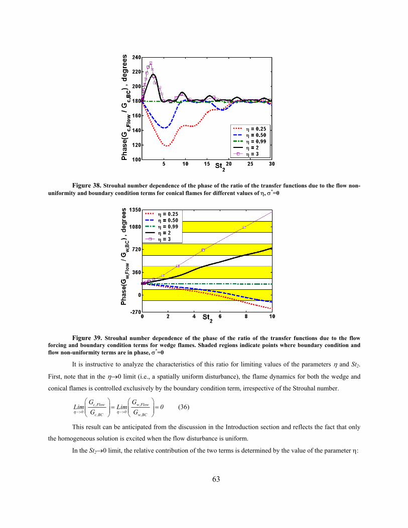
Figure 38. Strouhal number dependence of the phase of the ratio of the transfer functions due to the flow non-uniformity and boundary condition terms for conical flames for different values of η, σ*=0
Figure 39. Strouhal number dependence of the phase of the ratio of the transfer functions due to the flow forcing and boundary condition terms for wedge flames. Shaded regions indicate points where boundary condition and flow non-uniformity terms are in phase, σ*=0
It is instructive to analyze the characteristics of this ratio for limiting values of the parameters η and St2.
First, note that in the η→0 limit (i.e., a spatially uniform disturbance), the flame dynamics for both the wedge and
conical flames is controlled exclusively by the boundary condition term, irrespective of the Strouhal number.
c ,Flow w,Flow
0 0c,BC w,BC
G GLim Lim 0
G Gη η−> −>
= =
(36)
This result can be anticipated from the discussion in the Introduction section and reflects the fact that only
the homogeneous solution is excited when the flow disturbance is uniform.
In the St2→0 limit, the relative contribution of the two terms is determined by the value of the parameter η:
63
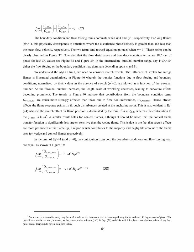
c ,Flow w,Flow
St 02 c,BC w,BC
G GLim
G Gη
−>
=
= − (37)
The boundary condition and flow forcing terms dominate when η<1 and η>1, respectively. For long flames
(β>>1), this physically corresponds to situations where the disturbance phase velocity is greater than and less than
the mean flow velocity, respectively. The two terms tend toward equal magnitudes when η = 1‡. These points can be
clearly observed in Figure 37. Note also that the flow disturbance and boundary condition terms are 180º out of
phase for low St2 values see Figure 38 and Figure 39. In the intermediate Strouhal number range, say 1<St2<10,
either the flow forcing or the boundary condition may dominate depending upon η and St2.
To understand the St2>>1 limit, we need to consider stretch effects. The influence of stretch for wedge
flames is illustrated quantitatively in Figure 40 wherein the transfer functions due to flow forcing and boundary
conditions, normalized by their values in the absence of stretch (σ*=0), are plotted as a function of the Strouhal
number. As the Strouhal number increases, the length scale of wrinkling decreases, leading to curvature effects
becoming prominent. The trends in Figure 40 indicate that contributions from the boundary condition term,
Gw,Area,BC, are much more strongly affected than those due to flow non-uniformities, Gw,Area,Flow. Hence, stretch
affects the flame response primarily through disturbances created at the anchoring point. This is also evident in Eq.
(24) wherein the stretch effect on flame position is dominated by the term σ*St in ζ1,BC whereas the contribution to
the ζ1,Flow is O~σ*. A similar result holds for conical flames, although it should be noted that the conical flame
transfer function is significantly less stretch sensitive than the wedge flame. This is due to the fact that stretch effects
are more prominent at the flame tip, a region which contributes to the majority and negligible amount of the flame
area for wedge and conical flames respectively.
In the limit of St2>>1 (and σ*=0), the contribution from both the boundary conditions and flow forcing term
are equal, as shown in Figure 37:
c ,Area ,Flow iSt22St2 c ,Area ,BC
GLim 1 i St e
Gσ ∗
−>∞
= − −
w,Area ,Flow i( 1 )St2 22St2 w,Area ,BC
GLim (1 St )e
Gησ −∗
−>∞
= − +
(38)
‡ Some care is required in analyzing this η=1 result, as the two terms tend to have equal magnitudes and are 180 degrees out of phase. The
overall response is not zero, however, as the common denominator (η-1) in Eqs. (31) and (34), which has been cancelled out when taking their ratio, causes their sum to have a non-zero value.
64
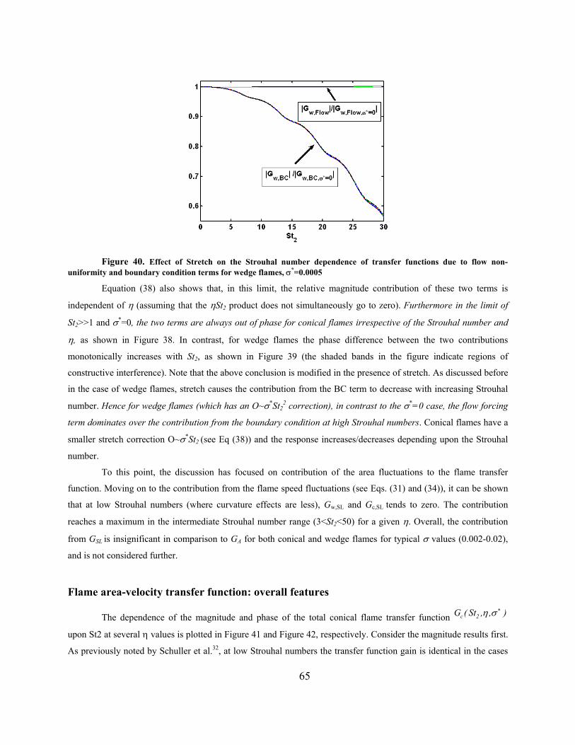
Figure 40. Effect of Stretch on the Strouhal number dependence of transfer functions due to flow non-uniformity and boundary condition terms for wedge flames, σ*=0.0005
Equation (38) also shows that, in this limit, the relative magnitude contribution of these two terms is
independent of η (assuming that the ηSt2 product does not simultaneously go to zero). Furthermore in the limit of
St2>>1 and σ*=0, the two terms are always out of phase for conical flames irrespective of the Strouhal number and
η, as shown in Figure 38. In contrast, for wedge flames the phase difference between the two contributions
monotonically increases with St2, as shown in Figure 39 (the shaded bands in the figure indicate regions of
constructive interference). Note that the above conclusion is modified in the presence of stretch. As discussed before
in the case of wedge flames, stretch causes the contribution from the BC term to decrease with increasing Strouhal
number. Hence for wedge flames (which has an O~σ*St22 correction), in contrast to the σ*=0 case, the flow forcing
term dominates over the contribution from the boundary condition at high Strouhal numbers. Conical flames have a
smaller stretch correction O~σ*St2 (see Eq (38)) and the response increases/decreases depending upon the Strouhal
number.
To this point, the discussion has focused on contribution of the area fluctuations to the flame transfer
function. Moving on to the contribution from the flame speed fluctuations (see Eqs. (31) and (34)), it can be shown
that at low Strouhal numbers (where curvature effects are less), Gw,SL and Gc,SL tends to zero. The contribution
reaches a maximum in the intermediate Strouhal number range (3<St2<50) for a given η. Overall, the contribution
from GSL is insignificant in comparison to GA for both conical and wedge flames for typical σ values (0.002-0.02),
and is not considered further.
Flame area-velocity transfer function: overall features
The dependence of the magnitude and phase of the total conical flame transfer function G (c 2St , , )η σ ∗
upon St2 at several η values is plotted in Figure 41 and Figure 42, respectively. Consider the magnitude results first.
As previously noted by Schuller et al.32, at low Strouhal numbers the transfer function gain is identical in the cases
65
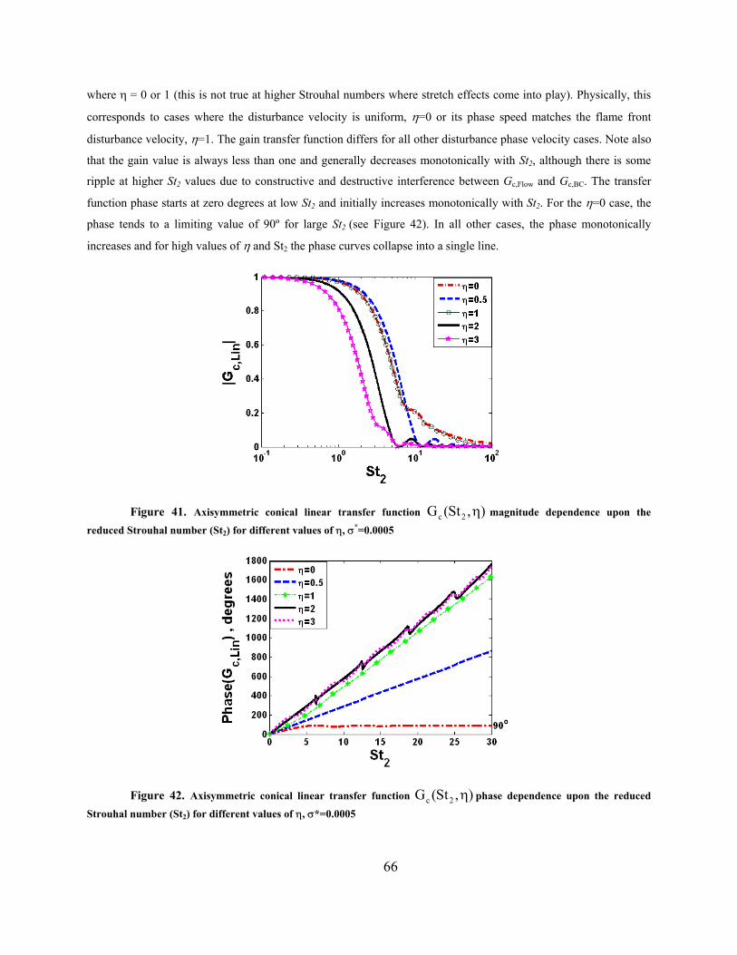
where η = 0 or 1 (this is not true at higher Strouhal numbers where stretch effects come into play). Physically, this
corresponds to cases where the disturbance velocity is uniform, η=0 or its phase speed matches the flame front
disturbance velocity, η=1. The gain transfer function differs for all other disturbance phase velocity cases. Note also
that the gain value is always less than one and generally decreases monotonically with St2, although there is some
ripple at higher St2 values due to constructive and destructive interference between Gc,Flow and Gc,BC. The transfer
function phase starts at zero degrees at low St2 and initially increases monotonically with St2. For the η=0 case, the
phase tends to a limiting value of 90º for large St2 (see Figure 42). In all other cases, the phase monotonically
increases and for high values of η and St2 the phase curves collapse into a single line.
Figure 41. Axisymmetric conical linear transfer function G (c 2St , )η magnitude dependence upon the
reduced Strouhal number (St2) for different values of η, σ*=0.0005
Figure 42. Axisymmetric conical linear transfer function G (c 2St , )η phase dependence upon the reduced
Strouhal number (St2) for different values of η, σ*=0.0005
66
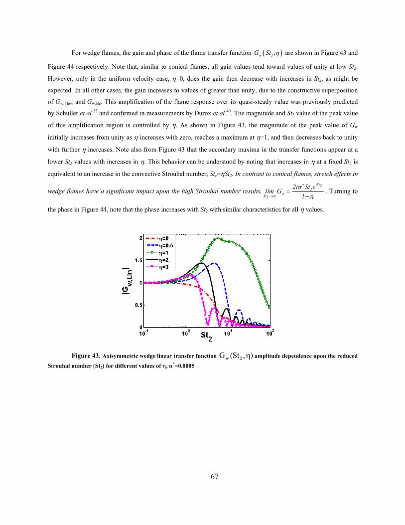
For wedge flames, the gain and phase of the flame transfer function ( )w 2t ,G S η are shown in Figure 43 and
Figure 44 respectively. Note that, similar to conical flames, all gain values tend toward values of unity at low St2.
However, only in the uniform velocity case, η=0, does the gain then decrease with increases in St2, as might be
expected. In all other cases, the gain increases to values of greater than unity, due to the constructive superposition
of Gw,Flow and Gw,Bc. This amplification of the flame response over its quasi-steady value was previously predicted
by Schuller et al.32 and confirmed in measurements by Durox et al.40. The magnitude and St2 value of the peak value
of this amplification region is controlled by η. As shown in Figure 43, the magnitude of the peak value of Gw
initially increases from unity as η increases with zero, reaches a maximum at η=1, and then decreases back to unity
with further η increases. Note also from Figure 43 that the secondary maxima in the transfer functions appear at a
lower St2 values with increases in η. This behavior can be understood by noting that increases in η at a fixed St2 is
equivalent to an increase in the convective Strouhal number, Stc=ηSt2. In contrast to conical flames, stretch effects in
wedge flames have a significant impact upon the high Strouhal number results,iSt2
22i St e1
ση
∗
=−wSt2
lim G→∞
. Turning to
the phase in Figure 44, note that the phase increases with St2 with similar characteristics for all η values.
Figure 43. Axisymmetric wedge linear transfer function G (w 2St , )η amplitude dependence upon the reduced
Strouhal number (St2) for different values of η, σ*=0.0005
67
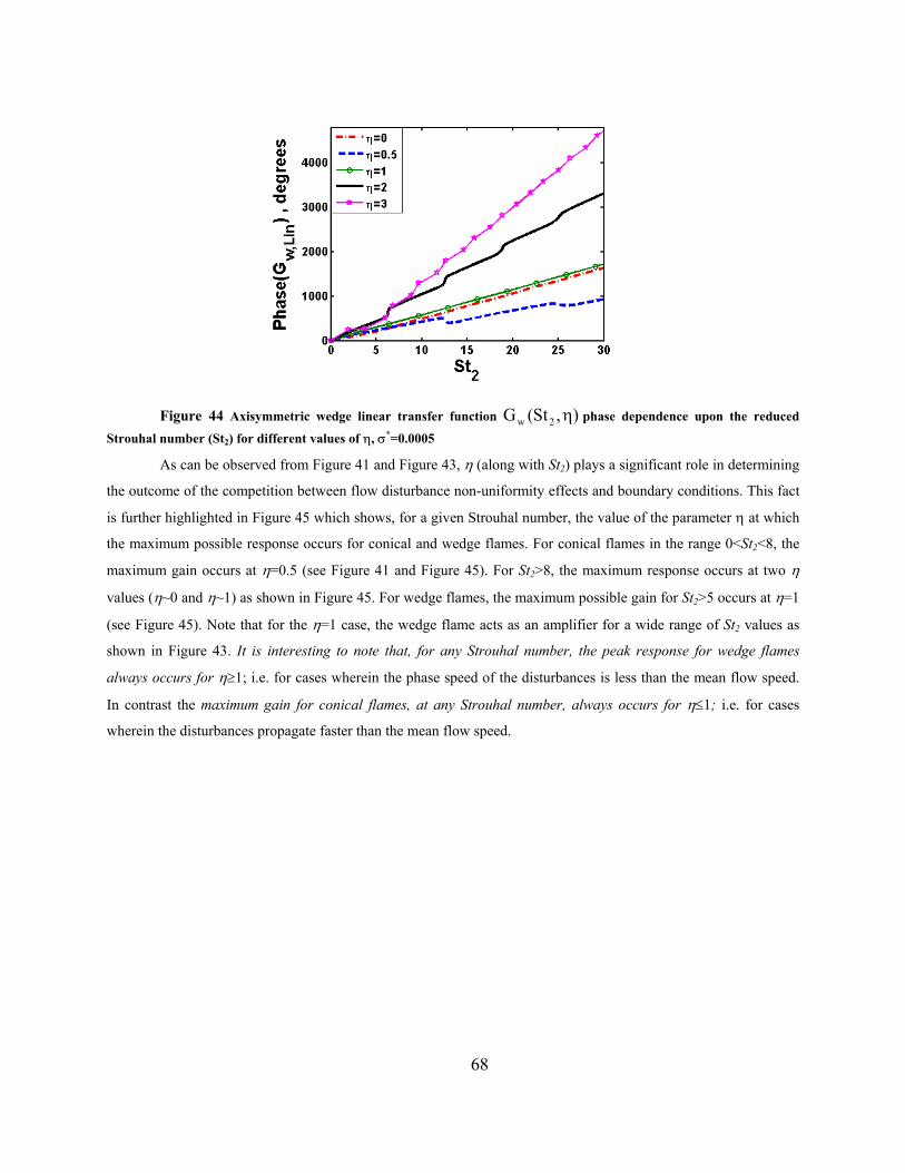
Figure 44 Axisymmetric wedge linear transfer function G (w 2St , )η phase dependence upon the reduced
Strouhal number (St2) for different values of η, σ*=0.0005
As can be observed from Figure 41 and Figure 43, η (along with St2) plays a significant role in determining
the outcome of the competition between flow disturbance non-uniformity effects and boundary conditions. This fact
is further highlighted in Figure 45 which shows, for a given Strouhal number, the value of the parameter η at which
the maximum possible response occurs for conical and wedge flames. For conical flames in the range 0<St2<8, the
maximum gain occurs at η=0.5 (see Figure 41 and Figure 45). For St2>8, the maximum response occurs at two η
values (η~0 and η~1) as shown in Figure 45. For wedge flames, the maximum possible gain for St2>5 occurs at η=1
(see Figure 45). Note that for the η=1 case, the wedge flame acts as an amplifier for a wide range of St2 values as
shown in Figure 43. It is interesting to note that, for any Strouhal number, the peak response for wedge flames
always occurs for η≥1; i.e. for cases wherein the phase speed of the disturbances is less than the mean flow speed.
In contrast the maximum gain for conical flames, at any Strouhal number, always occurs for η≤1; i.e. for cases
wherein the disturbances propagate faster than the mean flow speed.
68
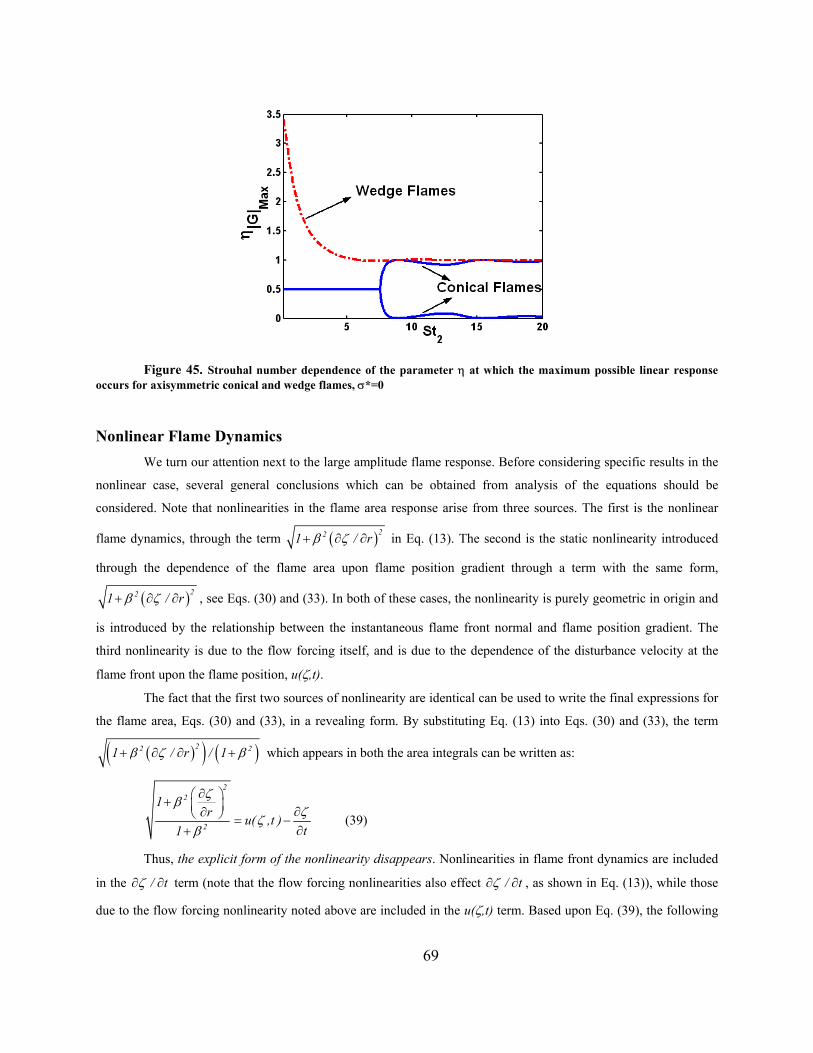
Figure 45. Strouhal number dependence of the parameter η at which the maximum possible linear response occurs for axisymmetric conical and wedge flames, σ*=0
Nonlinear Flame Dynamics We turn our attention next to the large amplitude flame response. Before considering specific results in the
nonlinear case, several general conclusions which can be obtained from analysis of the equations should be
considered. Note that nonlinearities in the flame area response arise from three sources. The first is the nonlinear
flame dynamics, through the term ( )221 /β ζ+ ∂ ∂r
)
in Eq. (13). The second is the static nonlinearity introduced
through the dependence of the flame area upon flame position gradient through a term with the same form,
( 221 /β ζ+ ∂ ∂r
)
, see Eqs. (30) and (33). In both of these cases, the nonlinearity is purely geometric in origin and
is introduced by the relationship between the instantaneous flame front normal and flame position gradient. The
third nonlinearity is due to the flow forcing itself, and is due to the dependence of the disturbance velocity at the
flame front upon the flame position, u(ζ,t).
The fact that the first two sources of nonlinearity are identical can be used to write the final expressions for
the flame area, Eqs. (30) and (33), in a revealing form. By substituting Eq. (13) into Eqs. (30) and (33), the term
( )( ) (221 / r / 1 2β ζ β+ ∂ ∂ + which appears in both the area integrals can be written as:
22
2
1r u( ,t )
t1
ζβζζ
β
∂ + ∂∂ = −∂+
(39)
Thus, the explicit form of the nonlinearity disappears. Nonlinearities in flame front dynamics are included
in the / tζ∂ term (note that the flow forcing nonlinearities also effect ∂ / tζ∂ ∂ , as shown in Eq. (13)), while those
due to the flow forcing nonlinearity noted above are included in the u(ζ,t) term. Based upon Eq. (39), the following
69
observations can be made regarding the effects of various parameters upon nonlinearity in the flame’s response to
flow perturbations.
Strouhal Number: At low Strouhal numbers, St, the unsteady term in Eq. (39) is negligible. Moreover, the
ζ dependence of the velocity field, u(ζ,t), is weak, at least for the velocity fields considered here. Thus, the flame
area’s velocity response remains linear for low Strouhal numbers, as St is the dimensionless ratio of the flame
response time to perturbation period. This point shows that the flame’s nonlinear area response is an intrinsically
dynamic phenomenon; its quasi-steady response is linear.
Flow Uniformity: Nonlinearities in the u(ζ,t) term are directly due to non-uniformity in flow disturbances.
Thus, the contribution of this term to flame area nonlinearities is suppressed in the η→0 limit.
Boundary conditions: If the flame remains anchored at the attachment point, as it is in this study, then
/ tζ∂ ∂ is identically zero at this point for all time. As such, the flame area perturbations in the vicinity of the
attachment point (where ζ≈0 ⇒ u≈u(0,t)) exhibit a linear dependence upon velocity amplitude. Nonlinearities only
arise at points of the flame that are spatially removed from the attachment point. As such, the axisymmetric conical
flame exhibits a more linear response than the axisymmetric wedge flame for comparable values of ε, since most
and very little, respectively, of the flame area is concentrated near the attachment point. This discussion also shows
the potential coupling between the flame kinematic and flame holding sources of nonlinearity.
Flame Aspect Ratio: The flame dynamics tend to linearity when β>>1; i.e., when the flame is very long.
This can be seen by noting that the left side of Eq. (13) becomes linear in this case:
( )221 / rβ ζ β ζ+ ∂ ∂ = ± ∂ ∂/ r . As such, the flame dynamics is approximately described by the
equation u( ,t )t rζ ζ ζ∂ ∂
± =∂ ∂
. In this case, the flame dynamics are linear, although the flow forcing term need not be.
This discussion shows that β is an important nonlinearity parameter for this problem; i.e., the flame’s area response
can be anticipated to exhibit a linear dependence upon the perturbation velocity for much larger ε values at large β
values.
Next, we derive an expression for the lowest order nonlinear correction to the flame area-velocity transfer
function by determining the response of a flame to a disturbance with an arbitrary phase velocity. Stretch effects are
not included here, but retained in the computations. Returning to the perturbation expansion for the flame position in
Eq. (21), the following equations describe the dynamics of the second and third order correction terms, ζ2 and ζ3: 2
2 2 11
(1 ) KSt Sin[ St{ K(1 r ) t }] 0t r 2 r
ζ ζ ζα αα ζ∂ ∂ ∂− − + + − − = ∂ ∂ ∂
3 2 2 223 3 1 1 2 1
2
K St(1 ) (1 ) Cos[ St{ K(1 r ) t }]t r 2 r r r 2
KSt Sin[ St{ K(1 r ) t }] 0
ζ ζ ζ ζ ζ ζα αα α α
ζ
∂ ∂ ∂ ∂ ∂− − + + − + − − ∂ ∂ ∂ ∂ ∂ + − − =
(40)
The solution of Eq. (40), subject to the boundary condition in Eq. (14), is given in Appendix C. In the
ensuing discussion, we focus upon the total heat release response. Defining the conical flame area-velocity transfer
70
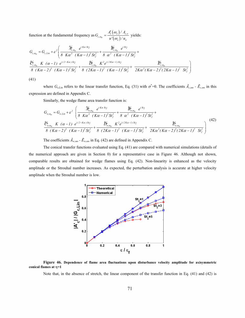
function at the fundamental frequency as( )( )
c o c,oc , o
o o
A / AG
u' / uω
ωω
′= yields:
i K St i St2 2c , c ,2 o o
c, c ,Lin 3 5 2 2 5 2o2 2
i ( 2 K ) St i ( 2K 1 ) St22 2c, c , c ,o o
3 5 2 2 5 2 3 3 22 2
A e B eG G
8 K ( K 1) St 8 ( K 1) St
C K ( 1) e D K e E8 ( K 2 ) ( K 1) St 8 ( 2K 1) ( K 1) St 2K ( K 2 ) ( 2K 1) St
αω ω
ω
α αω ω ω
εα α α α
α
α α α α α α α
− −
= + + + − −
−+ +− − − − − −
% %
% % %o
22
(41)
where Gc,Lin refers to the linear transfer function, Eq. (31) with σ*=0. The coefficients Ãc,ωo - Ẽc,ωo in this
expression are defined in Appendix C.
Similarly, the wedge flame area transfer function is:
i K St i St2 2w, w,2 o o
w, w,Lin 3 5 2 2 5 2o2 2
i ( 2 K ) St i ( 2K 1 ) St22 2w, w, w,o o
3 5 2 2 5 2 3 3 22 2
A e B eG G
8 K ( K 1) St 8 ( K 1) St
C K ( 1) e D K e E8 ( K 2 ) ( K 1) St 8 ( 2K 1) ( K 1) St 2K ( K 2 ) ( 2K 1) St
αω ω
ω
α αω ω ω
εα α α α
α
α α α α α α α
− −
= + + + − −
−+ +− − − − − −
% %
% % %o
22
(42)
The coefficients Ãw,ωo - Ẽw,ωo in Eq. (42) are defined in Appendix C.
The conical transfer functions evaluated using Eq. (41) are compared with numerical simulations (details of
the numerical approach are given in Section 0) for a representative case in Figure 46. Although not shown,
comparable results are obtained for wedge flames using Eq. (42). Non-linearity is enhanced as the velocity
amplitude or the Strouhal number increases. As expected, the perturbation analysis is accurate at higher velocity
amplitude when the Strouhal number is low.
Figure 46. Dependence of flame area fluctuations upon disturbance velocity amplitude for axisymmetric conical flames at η=1
Note that, in the absence of stretch, the linear component of the transfer function in Eq. (41) and (42) is
71
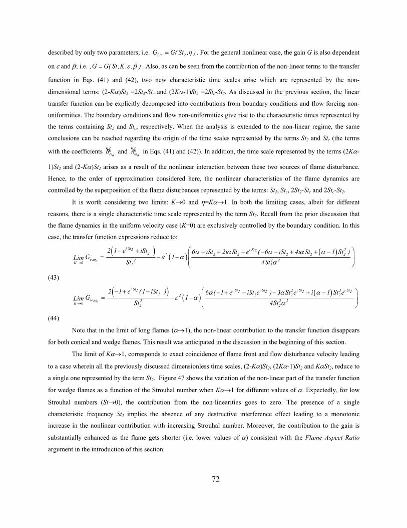
described by only two parameters; i.e. G GLin 2( St , )η= . For the general nonlinear case, the gain G is also dependent
on ε and β; i.e. , G G( St,K , , )ε β=
oB
. Also, as can be seen from the contribution of the non-linear terms to the transfer
function in Eqs. (41) and (42), two new characteristic time scales arise which are represented by the non-
dimensional terms: (2-Kα)St2 =2St2-Stc and (2Kα-1)St2 =2Stc-St2. As discussed in the previous section, the linear
transfer function can be explicitly decomposed into contributions from boundary conditions and flow forcing non-
uniformities. The boundary conditions and flow non-uniformities give rise to the characteristic times represented by
the terms containing St2 and Stc, respectively. When the analysis is extended to the non-linear regime, the same
conclusions can be reached regarding the origin of the time scales represented by the terms St2 and Stc (the terms
with the coefficients ω%
o and Aω
% in Eqs. (41) and (42)). In addition, the time scale represented by the terms (2Kα-
1)St2 and (2-Kα)St2 arises as a result of the nonlinear interaction between these two sources of flame disturbance.
Hence, to the order of approximation considered here, the nonlinear characteristics of the flame dynamics are
controlled by the superposition of the flame disturbances represented by the terms: St2, Stc, 2St2-Stc and 2Stc-St2.
It is worth considering two limits: K→0 and η=Kα→1. In both the limiting cases, albeit for different
reasons, there is a single characteristic time scale represented by the term St2. Recall from the prior discussion that
the flame dynamics in the uniform velocity case (K=0) are exclusively controlled by the boundary condition. In this
case, the transfer function expressions reduce to:
( )( ) ( )i St2 i St 22
2 2 2 2 2 22c , 2 2 2oK 0 2 2
2 1 e iSt 6 iSt 2i St e ( 6 iSt 4i St 1 St )G 1Lim
St 4Stω
α α α α αε α
α→
− + + + + − − + + −= − −
(43)
( )( ) ( )i St2 i St i St i St i St2 32 2 2
2 2 2 22w, 2 2 2oK 0 2 2
2 1 e (1 iSt ) 6 ( 1 e iSt e ) 3 St e i 1 St eG 1Lim
St 4Stω
α α αε α
α→
− + − − + − − + −= − −
2
(44)
Note that in the limit of long flames (α→1), the non-linear contribution to the transfer function disappears
for both conical and wedge flames. This result was anticipated in the discussion in the beginning of this section.
The limit of Kα→1, corresponds to exact coincidence of flame front and flow disturbance velocity leading
to a case wherein all the previously discussed dimensionless time scales, (2-Kα)St2, (2Kα-1)St2 and KαSt2, reduce to
a single one represented by the term St2. Figure 47 shows the variation of the non-linear part of the transfer function
for wedge flames as a function of the Strouhal number when Kα→1 for different values of α. Expectedly, for low
Strouhal numbers (St→0), the contribution from the non-linearities goes to zero. The presence of a single
characteristic frequency St2 implies the absence of any destructive interference effect leading to a monotonic
increase in the nonlinear contribution with increasing Strouhal number. Moreover, the contribution to the gain is
substantially enhanced as the flame gets shorter (i.e. lower values of α) consistent with the Flame Aspect Ratio
argument in the introduction of this section.
72
Figure 47. Dependence of non-linear part of the transfer function for axisymmetric wedge flames at η=1
Hence the presence of a single characteristic time scale, for the uniform velocity (K=0) and the η=Kα→1
case, causes the nonlinear contribution to monotonically increase with increasing Strouhal number and/or
decreasing flame aspect ratio. As discussed further below, it is only for these two cases that the non-linearities
always lead to a reduction in the magnitude of the total transfer function. These conclusions are valid even at higher
velocity amplitudes as shown by numerical simulations in Figure 48-Figure 51 which plot the St2 dependence of the
gain and phase of the nonlinear transfer function upon St2 at several η values. The gain transfer functions are
normalized by their linear values, G/GLin. Results are shown for two convective wave speeds, η=0 and η=1, but the
same β=1 value. Thus, these results allow for a convenient comparison of the effects of nonlinearities from
boundary conditions alone, and the combined effect of boundary conditions and flow disturbance non-uniformity.
Consider the gain curves first, Figure 48 and Figure 50. As predicted earlier, the response tends to its linear value in
all cases at low St2. In the η=0 case, nonlinear effects are more apparent at high St2. For the wedge flame in Figure
50 the response is considerably nonlinear even at moderate values of Strouhal number. The enhanced nonlinear
response of wedge over cone flames is explained by the Boundary Conditions argument discussed earlier.
Turning to the η=1 case, note the substantial reduction in flame area relative to its linear value; i.e., there is
a substantial degree of gain saturation. Although plotted in a different form, the resulting gain curves look quite
similar to the qualitative plot of Hn(A) in Figure 29. In agreement with the Strouhal Number argument discussed
earlier, the degree of nonlinearity increases with St2. As shown in Figure 48 and Figure 50, the gain for the conical
and wedge flames decreases by about 60% and 70% respectively (at ε=εf in the St2= 20 and η= 1 case). In contrast,
the gain never drops below 5% of its linear value for conical flames and 35% of its linear value for wedge flames in
the η=0 case. Moreover, unlike the η=0 case, the phase of the area response for both the conical and wedge flames
exhibits a strong amplitude dependence, as shown in Figure 49 and Figure 51 respectively. These results indicate the
extent to which flow non-uniformities can significantly modify the nonlinear flame response.
73
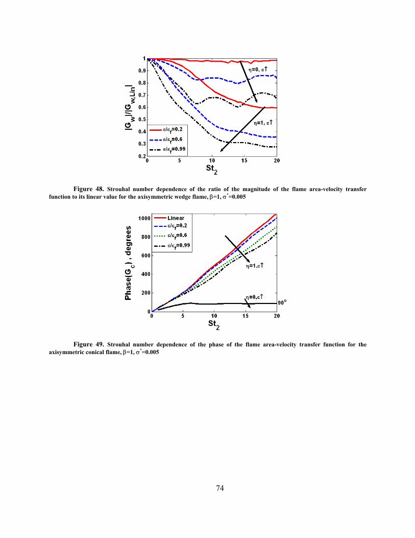
Figure 48. Strouhal number dependence of the ratio of the magnitude of the flame area-velocity transfer function to its linear value for the axisymmetric wedge flame, β=1, σ*=0.005
Figure 49. Strouhal number dependence of the phase of the flame area-velocity transfer function for the axisymmetric conical flame, β=1, σ*=0.005
74
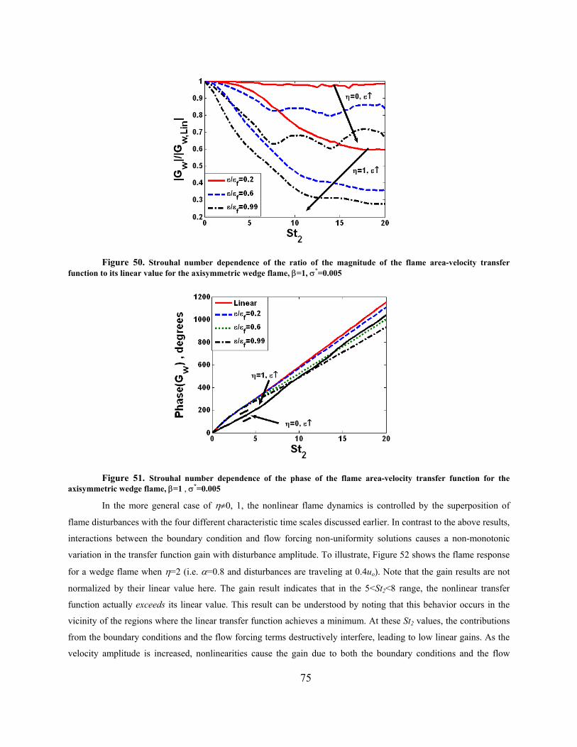
Figure 50. Strouhal number dependence of the ratio of the magnitude of the flame area-velocity transfer function to its linear value for the axisymmetric wedge flame, β=1, σ*=0.005
Figure 51. Strouhal number dependence of the phase of the flame area-velocity transfer function for the axisymmetric wedge flame, β=1 , σ*=0.005
In the more general case of η≠0, 1, the nonlinear flame dynamics is controlled by the superposition of
flame disturbances with the four different characteristic time scales discussed earlier. In contrast to the above results,
interactions between the boundary condition and flow forcing non-uniformity solutions causes a non-monotonic
variation in the transfer function gain with disturbance amplitude. To illustrate, Figure 52 shows the flame response
for a wedge flame when η=2 (i.e. α=0.8 and disturbances are traveling at 0.4uo). Note that the gain results are not
normalized by their linear value here. The gain result indicates that in the 5<St2<8 range, the nonlinear transfer
function actually exceeds its linear value. This result can be understood by noting that this behavior occurs in the
vicinity of the regions where the linear transfer function achieves a minimum. At these St2 values, the contributions
from the boundary conditions and the flow forcing terms destructively interfere, leading to low linear gains. As the
velocity amplitude is increased, nonlinearities cause the gain due to both the boundary conditions and the flow
75
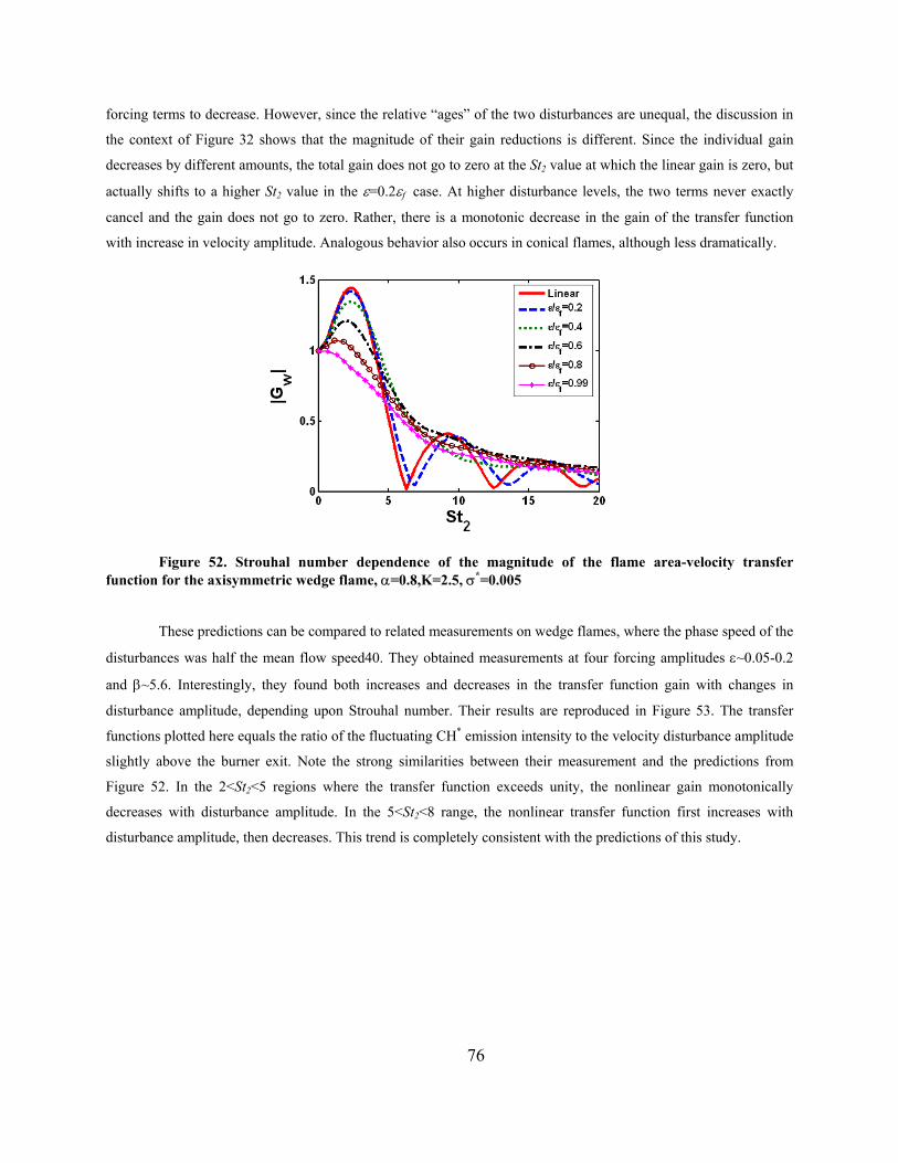
forcing terms to decrease. However, since the relative “ages” of the two disturbances are unequal, the discussion in
the context of Figure 32 shows that the magnitude of their gain reductions is different. Since the individual gain
decreases by different amounts, the total gain does not go to zero at the St2 value at which the linear gain is zero, but
actually shifts to a higher St2 value in the ε=0.2εf case. At higher disturbance levels, the two terms never exactly
cancel and the gain does not go to zero. Rather, there is a monotonic decrease in the gain of the transfer function
with increase in velocity amplitude. Analogous behavior also occurs in conical flames, although less dramatically.
Figure 52. Strouhal number dependence of the magnitude of the flame area-velocity transfer function for the axisymmetric wedge flame, α=0.8,K=2.5, σ*=0.005
These predictions can be compared to related measurements on wedge flames, where the phase speed of the
disturbances was half the mean flow speed40. They obtained measurements at four forcing amplitudes ε~0.05-0.2
and β~5.6. Interestingly, they found both increases and decreases in the transfer function gain with changes in
disturbance amplitude, depending upon Strouhal number. Their results are reproduced in Figure 53. The transfer
functions plotted here equals the ratio of the fluctuating CH* emission intensity to the velocity disturbance amplitude
slightly above the burner exit. Note the strong similarities between their measurement and the predictions from
Figure 52. In the 2<St2<5 regions where the transfer function exceeds unity, the nonlinear gain monotonically
decreases with disturbance amplitude. In the 5<St2<8 range, the nonlinear transfer function first increases with
disturbance amplitude, then decreases. This trend is completely consistent with the predictions of this study.
76
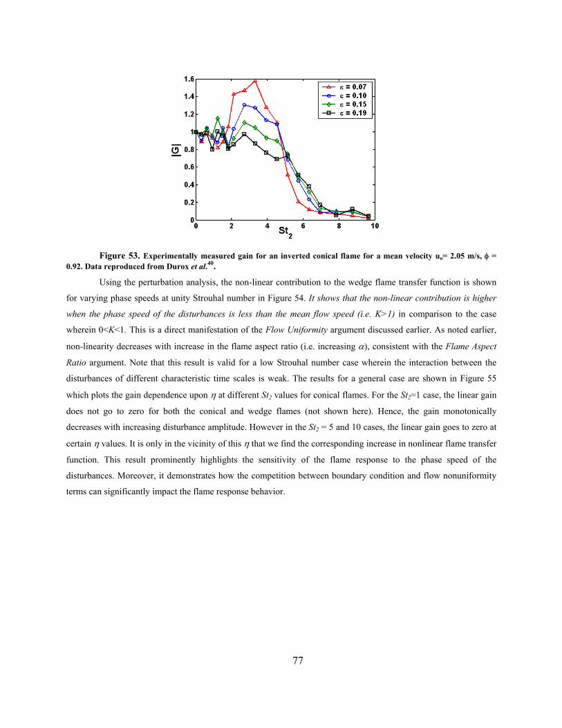
Figure 53. Experimentally measured gain for an inverted conical flame for a mean velocity uo= 2.05 m/s, φ = 0.92. Data reproduced from Durox et al.40.
Using the perturbation analysis, the non-linear contribution to the wedge flame transfer function is shown
for varying phase speeds at unity Strouhal number in Figure 54. It shows that the non-linear contribution is higher
when the phase speed of the disturbances is less than the mean flow speed (i.e. K>1) in comparison to the case
wherein 0<K<1. This is a direct manifestation of the Flow Uniformity argument discussed earlier. As noted earlier,
non-linearity decreases with increase in the flame aspect ratio (i.e. increasing α), consistent with the Flame Aspect
Ratio argument. Note that this result is valid for a low Strouhal number case wherein the interaction between the
disturbances of different characteristic time scales is weak. The results for a general case are shown in Figure 55
which plots the gain dependence upon η at different St2 values for conical flames. For the St2=1 case, the linear gain
does not go to zero for both the conical and wedge flames (not shown here). Hence, the gain monotonically
decreases with increasing disturbance amplitude. However in the St2 = 5 and 10 cases, the linear gain goes to zero at
certain η values. It is only in the vicinity of this η that we find the corresponding increase in nonlinear flame transfer
function. This result prominently highlights the sensitivity of the flame response to the phase speed of the
disturbances. Moreover, it demonstrates how the competition between boundary condition and flow nonuniformity
terms can significantly impact the flame response behavior.
77
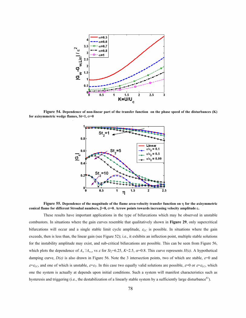
Figure 54. Dependence of non-linear part of the transfer function on the phase speed of the disturbances (K) for axisymmetric wedge flames, St=1, σ=0
Figure 55. Dependence of the magnitude of the flame area-velocity transfer function on η for the axisymmetric conical flame for different Strouhal numbers, β=8, σ=0. Arrow points towards increasing velocity amplitude ε.
These results have important applications in the type of bifurcations which may be observed in unstable
combustors. In situations where the gain curves resemble that qualitatively shown in Figure 29, only supercritical
bifurcations will occur and a single stable limit cycle amplitude, εLC is possible. In situations where the gain
exceeds, then is less than, the linear gain (see Figure 52); i.e., it exhibits an inflection point, multiple stable solutions
for the instability amplitude may exist, and sub-critical bifurcations are possible. This can be seen from Figure 56,
which plots the dependence of Aw’/Aw,o vs ε for St2=6.25, K=2.5, α=0.8. This curve represents H(ε). A hypothetical
damping curve, D(ε) is also drawn in Figure 56. Note the 3 intersection points, two of which are stable, ε=0 and
ε=εLC, and one of which is unstable, ε=εT. In this case two equally valid solutions are possible, ε=0 or ε=εLC, which
one the system is actually at depends upon initial conditions. Such a system will manifest characteristics such as
hysteresis and triggering (i.e., the destabilization of a linearly stable system by a sufficiently large disturbance81).
78
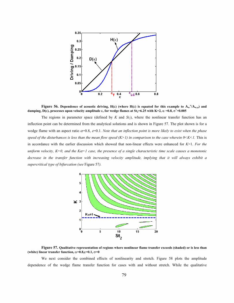
Figure 56. Dependence of acoustic driving, H(ε) (where H(ε) is equated for this example to Aw’/Aw,o) and damping, D(ε), processes upon velocity amplitude ε, for wedge flames at St2=6.25 with K=2, α =0.8, σ*=0.005
The regions in parameter space (defined by K and St2), where the nonlinear transfer function has an
inflection point can be determined from the analytical solutions and is shown in Figure 57. The plot shown is for a
wedge flame with an aspect ratio α=0.8, ε=0.1. Note that an inflection point is more likely to exist when the phase
speed of the disturbances is less than the mean flow speed (K>1) in comparison to the case wherein 0<K<1. This is
in accordance with the earlier discussion which showed that non-linear effects were enhanced for K>1. For the
uniform velocity, K=0, and the Kα=1 case, the presence of a single characteristic time scale causes a monotonic
decrease in the transfer function with increasing velocity amplitude, implying that it will always exhibit a
supercritical type of bifurcation (see Figure 57).
Figure 57. Qualitative representation of regions where nonlinear flame transfer exceeds (shaded) or is less than (white) linear transfer function, α=0.8,ε=0.1, σ=0
We next consider the combined effects of nonlinearity and stretch. Figure 58 plots the amplitude
dependence of the wedge flame transfer function for cases with and without stretch. While the qualitative
79
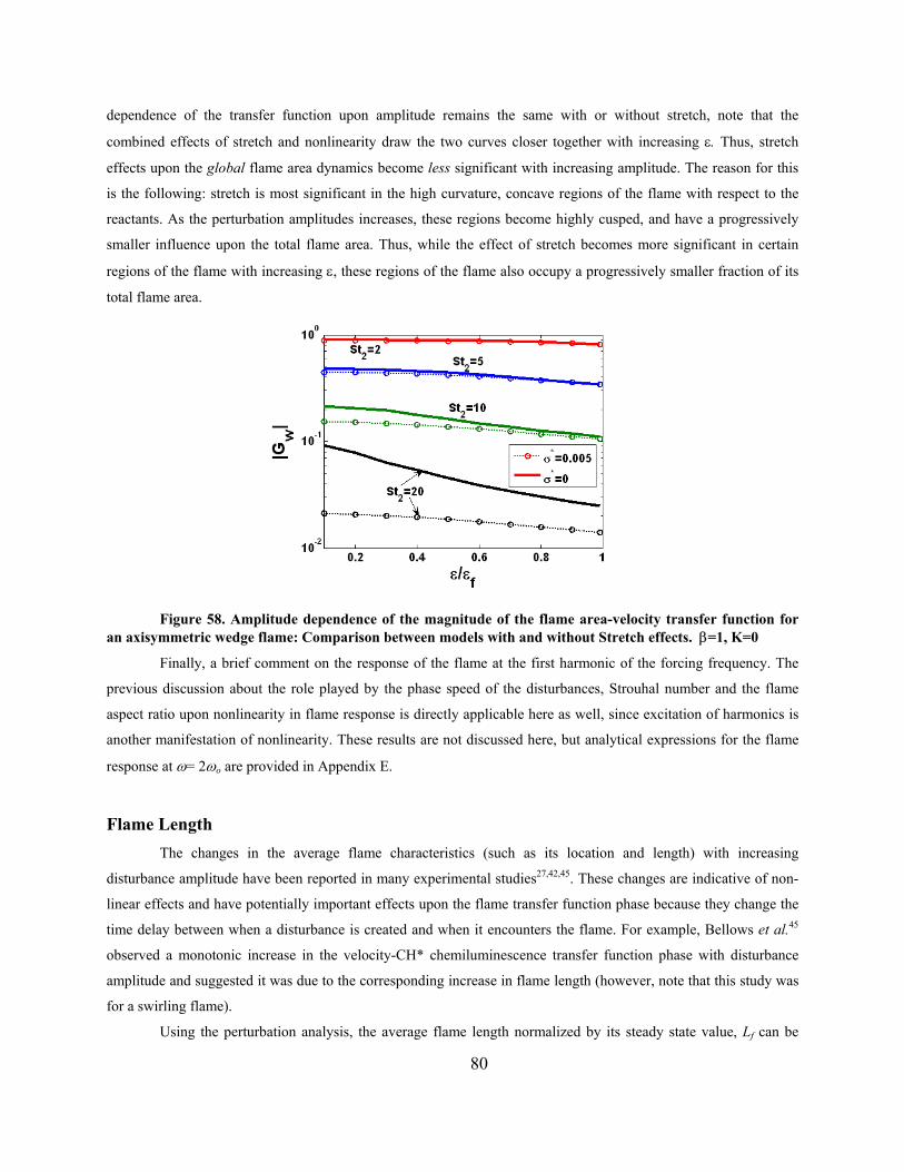
dependence of the transfer function upon amplitude remains the same with or without stretch, note that the
combined effects of stretch and nonlinearity draw the two curves closer together with increasing ε. Thus, stretch
effects upon the global flame area dynamics become less significant with increasing amplitude. The reason for this
is the following: stretch is most significant in the high curvature, concave regions of the flame with respect to the
reactants. As the perturbation amplitudes increases, these regions become highly cusped, and have a progressively
smaller influence upon the total flame area. Thus, while the effect of stretch becomes more significant in certain
regions of the flame with increasing ε, these regions of the flame also occupy a progressively smaller fraction of its
total flame area.
Figure 58. Amplitude dependence of the magnitude of the flame area-velocity transfer function for an axisymmetric wedge flame: Comparison between models with and without Stretch effects. β=1, K=0
Finally, a brief comment on the response of the flame at the first harmonic of the forcing frequency. The
previous discussion about the role played by the phase speed of the disturbances, Strouhal number and the flame
aspect ratio upon nonlinearity in flame response is directly applicable here as well, since excitation of harmonics is
another manifestation of nonlinearity. These results are not discussed here, but analytical expressions for the flame
response at ω= 2ωo are provided in Appendix E.
Flame Length The changes in the average flame characteristics (such as its location and length) with increasing
disturbance amplitude have been reported in many experimental studies27,42,45. These changes are indicative of non-
linear effects and have potentially important effects upon the flame transfer function phase because they change the
time delay between when a disturbance is created and when it encounters the flame. For example, Bellows et al.45
observed a monotonic increase in the velocity-CH* chemiluminescence transfer function phase with disturbance
amplitude and suggested it was due to the corresponding increase in flame length (however, note that this study was
for a swirling flame).
Using the perturbation analysis, the average flame length normalized by its steady state value, Lf can be
80
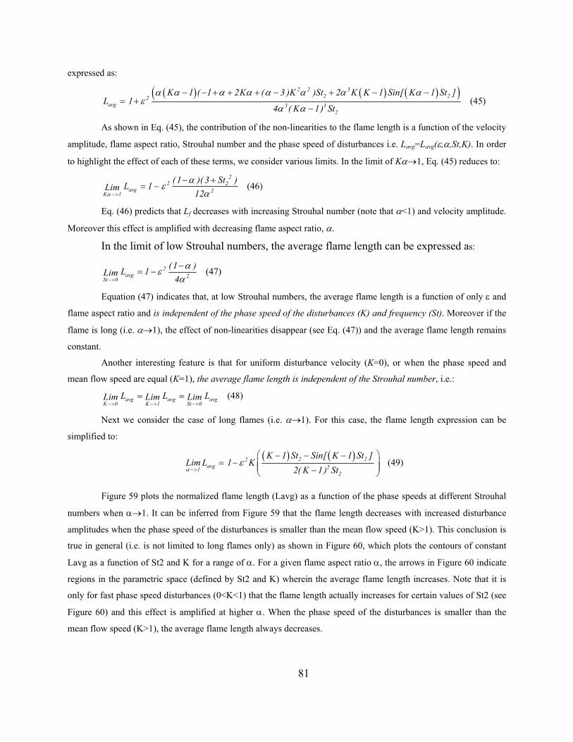
expressed as:
( ) ( ) ( )( )2 2 32 22
avg 3 32
K 1 ( 1 2K ( 3 )K )St 2 K K 1 Sin[ K 1 St ]L 1
4 ( K 1) St
α α α α α α α αε
α α
− − + + + − + − −= +
− (45)
As shown in Eq. (45), the contribution of the non-linearities to the flame length is a function of the velocity
amplitude, flame aspect ratio, Strouhal number and the phase speed of disturbances i.e. Lavg=Lavg(ε,α,St,K). In order
to highlight the effect of each of these terms, we consider various limits. In the limit of Kα→1, Eq. (45) reduces to: 2
2 2avg 2K 1
(1 )( 3 St )L 1Lim
12α
αε
α−>
− += − (46)
Eq. (46) predicts that Lf decreases with increasing Strouhal number (note that α<1) and velocity amplitude.
Moreover this effect is amplified with decreasing flame aspect ratio, α.
In the limit of low Strouhal numbers, the average flame length can be expressed as:
2avg 2St 0
(1 )L 1Lim4
αεα−>
−= − (47)
Equation (47) indicates that, at low Strouhal numbers, the average flame length is a function of only ε and
flame aspect ratio and is independent of the phase speed of the disturbances (K) and frequency (St). Moreover if the
flame is long (i.e. α→1), the effect of non-linearities disappear (see Eq. (47)) and the average flame length remains
constant.
Another interesting feature is that for uniform disturbance velocity (K=0), or when the phase speed and
mean flow speed are equal (K=1), the average flame length is independent of the Strouhal number, i.e.:
avg avg avgK 0 K 1 St 0
L LLim Lim Lim−> −> −>
= = L (48)
Next we consider the case of long flames (i.e. α→1). For this case, the flame length expression can be
simplified to:
( ) ( )2 22avg 21
2
K 1 St Sin[ K 1 St ]Lim L 1 K
2( K 1) Stαε
−>
− − −= − −
(49)
Figure 59 plots the normalized flame length (Lavg) as a function of the phase speeds at different Strouhal
numbers when α→1. It can be inferred from Figure 59 that the flame length decreases with increased disturbance
amplitudes when the phase speed of the disturbances is smaller than the mean flow speed (K>1). This conclusion is
true in general (i.e. is not limited to long flames only) as shown in Figure 60, which plots the contours of constant
Lavg as a function of St2 and K for a range of α. For a given flame aspect ratio α, the arrows in Figure 60 indicate
regions in the parametric space (defined by St2 and K) wherein the average flame length increases. Note that it is
only for fast phase speed disturbances (0<K<1) that the flame length actually increases for certain values of St2 (see
Figure 60) and this effect is amplified at higher α. When the phase speed of the disturbances is smaller than the
mean flow speed (K>1), the average flame length always decreases.
81
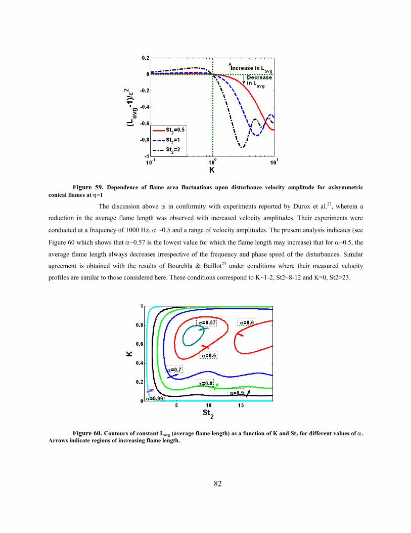
Figure 59. Dependence of flame area fluctuations upon disturbance velocity amplitude for axisymmetric conical flames at η=1
The discussion above is in conformity with experiments reported by Durox et al.27, wherein a
reduction in the average flame length was observed with increased velocity amplitudes. Their experiments were
conducted at a frequency of 1000 Hz, α ~0.5 and a range of velocity amplitudes. The present analysis indicates (see
Figure 60 which shows that α~0.57 is the lowest value for which the flame length may increase) that for α~0.5, the
average flame length always decreases irrespective of the frequency and phase speed of the disturbances. Similar
agreement is obtained with the results of Bourehla & Baillot25 under conditions where their measured velocity
profiles are similar to those considered here. These conditions correspond to K~1-2, St2~8-12 and K=0, St2>23.
Figure 60. Contours of constant Lavg (average flame length) as a function of K and St2 for different values of α. Arrows indicate regions of increasing flame length.
82
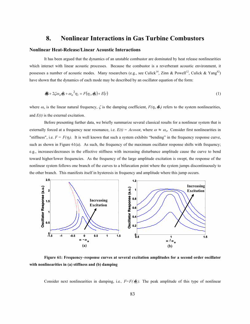
8. Nonlinear Interactions in Gas Turbine Combustors
Nonlinear Heat-Release/Linear Acoustic Interactions
It has been argued that the dynamics of an unstable combustor are dominated by heat release nonlinearities
which interact with linear acoustic processes. Because the combustor is a reverberant acoustic environment, it
possesses a number of acoustic modes. Many researchers (e.g., see Culick14, Zinn & Powell12, Culick & Yang82)
have shown that the dynamics of each mode may be described by an oscillator equation of the form:
( ) ( )tEF iiioioi +=++ ηηηωηζωη &&&& ,2 2 (1)
where ωo is the linear natural frequency, ζ is the damping coefficient, F(ηi,η&i) refers to the system nonlinearities,
and E(t) is the external excitation.
Before presenting further data, we briefly summarize several classical results for a nonlinear system that is
externally forced at a frequency near resonance, i.e. E(t) = Acosωt, where ω ≈ ωο. Consider first nonlinearities in
"stiffness", i.e. F = F(ηi). It is well known that such a system exhibits “bending” in the frequency response curve,
such as shown in Figure 61(a). As such, the frequency of the maximum oscillator response shifts with frequency;
e.g., increases/decreases in the effective stiffness with increasing disturbance amplitude cause the curve to bend
toward higher/lower frequencies. As the frequency of the large amplitude excitation is swept, the response of the
nonlinear system follows one branch of the curves to a bifurcation point where the system jumps discontinuously to
the other branch. This manifests itself in hysteresis in frequency and amplitude where this jump occurs.
-1.5 -1 -0.5 0 0.5 1 1.50
0.5
1
1.5
2
2.5
ω - ω o
Osc
illat
or R
espo
nse
(a.u
.)
0.5 1 1.50
0.2
0.4
0.6
0.8
1
1.2
ω / ω o
Osc
illat
or R
espo
nse
(a.u
.)
(a) (b)
Increasing Excitation
Increasing Excitation
-1.5 -1 -0.5 0 0.5 1 1.50
0.5
1
1.5
2
2.5
ω - ω o
Osc
illat
or R
espo
nse
(a.u
.)
0.5 1 1.50
0.2
0.4
0.6
0.8
1
1.2
ω / ω o
Osc
illat
or R
espo
nse
(a.u
.)
(a) (b)
Increasing Excitation
Increasing Excitation
Figure 61: Frequency–response curves at several excitation amplitudes for a second order oscillator
with nonlinearities in (a) stiffness and (b) damping
Consider next nonlinearities in damping, i.e., F=F( iη&). The peak amplitude of this type of nonlinear
83
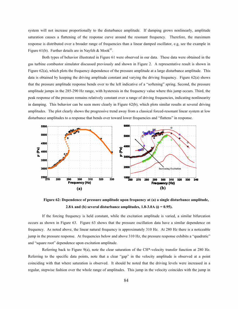
system will not increase proportionally to the disturbance amplitude. If damping grows nonlinearly, amplitude
saturation causes a flattening of the response curve around the resonant frequency. Therefore, the maximum
response is distributed over a broader range of frequencies than a linear damped oscillator, e.g, see the example in
Figure 61(b). Further details are in Nayfeh & Mook83.
Both types of behavior illustrated in Figure 61 were observed in our data. These data were obtained in the
gas turbine combustor simulator discussed previously and shown in Figure 2. A representative result is shown in
Figure 62(a), which plots the frequency dependence of the pressure amplitude at a large disturbance amplitude. This
data is obtained by keeping the driving amplitude constant and varying the driving frequency. Figure 62(a) shows
that the pressure amplitude response bends over to the left indicative of a “softening” spring. Second, the pressure
amplitude jumps in the 285-290 Hz range, with hysteresis in the frequency value where this jump occurs. Third, the
peak response of the pressure remains relatively constant over a range of driving frequencies, indicating nonlinearity
in damping. This behavior can be seen more clearly in Figure 62(b), which plots similar results at several driving
amplitudes. The plot clearly shows the progressive trend away from a classical forced-resonant linear system at low
disturbance amplitudes to a response that bends over toward lower frequencies and “flattens” in response.
270 280 290 300 310 320 3302500
3000
3500
4000
4500
5000
5500
Frequency (Hz)
p ′ (P
a)
(a) (b)
260 270 280 290 300 310 320 330 3401000
2000
3000
4000
5000
6000
Frequency (Hz)
p ′ (P
a)
Increasing Excitation
260 270 280 290 300 310 320 330 3401000
2000
3000
4000
5000
6000
Frequency (Hz)
p ′ (P
a)
260 270 280 290 300 310 320 330 3401000
2000
3000
4000
5000
6000
Frequency (Hz)
p ′ (P
a)
Increasing Excitation
270 280 290 300 310 320 3302500
3000
3500
4000
4500
5000
5500
Frequency (Hz)
p ′ (P
a)
270 280 290 300 310 320 3302500
3000
3500
4000
4500
5000
5500
Frequency (Hz)
p ′ (P
a)
(a) (b)
260 270 280 290 300 310 320 330 3401000
2000
3000
4000
5000
6000
Frequency (Hz)
p ′ (P
a)
Increasing Excitation
260 270 280 290 300 310 320 330 3401000
2000
3000
4000
5000
6000
Frequency (Hz)
p ′ (P
a)
260 270 280 290 300 310 320 330 3401000
2000
3000
4000
5000
6000
Frequency (Hz)
p ′ (P
a)
Increasing Excitation
Figure 62: Dependence of pressure amplitude upon frequency at (a) a single disturbance amplitude,
2.8A and (b) several disturbance amplitudes, 1.8-3.0A (φ = 0.95).
If the forcing frequency is held constant, while the excitation amplitude is varied, a similar bifurcation
occurs as shown in Figure 63. Figure 63 shows that the pressure oscillation data have a similar dependence on
frequency. As noted above, the linear natural frequency is approximately 310 Hz. At 280 Hz there is a noticeable
jump in the pressure response. At frequencies below and above 310 Hz, the pressure response exhibits a “quadratic”
and “square root” dependence upon excitation amplitude.
Referring back to Figure 9(a), note the clear saturation of the CH*-velocity transfer function at 280 Hz.
Referring to the specific data points, note that a clear “gap” in the velocity amplitude is observed at a point
coinciding with that where saturation is observed. It should be noted that the driving levels were increased in a
regular, stepwise fashion over the whole range of amplitudes. This jump in the velocity coincides with the jump in
84
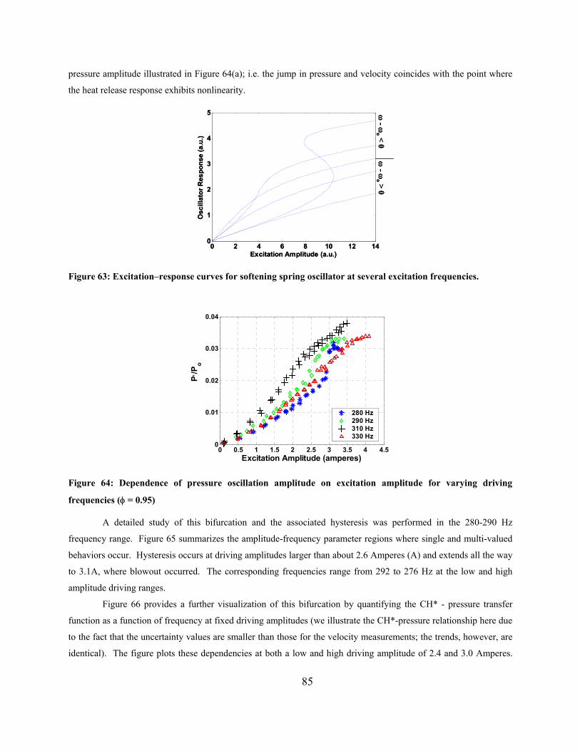
pressure amplitude illustrated in Figure 64(a); i.e. the jump in pressure and velocity coincides with the point where
the heat release response exhibits nonlinearity.
0 2 4 6 8 10 12 140
1
2
3
4
5
Excitation Amplitude (a.u.)
Osc
illat
or R
espo
nse
(a.u
.)ω
-ωo < 0
ω -ω
o > 0
0 2 4 6 8 10 12 140
1
2
3
4
5
Excitation Amplitude (a.u.)
Osc
illat
or R
espo
nse
(a.u
.)ω
-ωo < 0
ω -ω
o > 0
Figure 63: Excitation–response curves for softening spring oscillator at several excitation frequencies.
0 0.5 1 1.5 2 2.5 3 3.5 4 4.50
0.01
0.02
0.03
0.04
Excitation Amplitude (amperes)
P ′/P
o
280 Hz290 Hz310 Hz330 Hz
Figure 64: Dependence of pressure oscillation amplitude on excitation amplitude for varying driving
frequencies (φ = 0.95)
A detailed study of this bifurcation and the associated hysteresis was performed in the 280-290 Hz
frequency range. Figure 65 summarizes the amplitude-frequency parameter regions where single and multi-valued
behaviors occur. Hysteresis occurs at driving amplitudes larger than about 2.6 Amperes (A) and extends all the way
to 3.1A, where blowout occurred. The corresponding frequencies range from 292 to 276 Hz at the low and high
amplitude driving ranges.
Figure 66 provides a further visualization of this bifurcation by quantifying the CH* - pressure transfer
function as a function of frequency at fixed driving amplitudes (we illustrate the CH*-pressure relationship here due
to the fact that the uncertainty values are smaller than those for the velocity measurements; the trends, however, are
identical). The figure plots these dependencies at both a low and high driving amplitude of 2.4 and 3.0 Amperes.
85
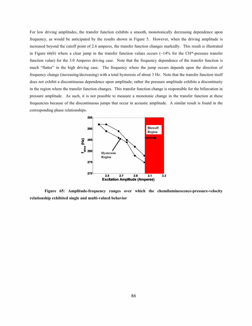
For low driving amplitudes, the transfer function exhibits a smooth, monotonically decreasing dependence upon
frequency, as would be anticipated by the results shown in Figure 5. However, when the driving amplitude is
increased beyond the cutoff point of 2.6 amperes, the transfer function changes markedly. This result is illustrated
in Figure 66(b) where a clear jump in the transfer function values occurs (~14% for the CH*-pressure transfer
function value) for the 3.0 Amperes driving case. Note that the frequency dependence of the transfer function is
much “flatter” in the high driving case. The frequency where the jump occurs depends upon the direction of
frequency change (increasing/decreasing) with a total hysteresis of about 3 Hz. Note that the transfer function itself
does not exhibit a discontinuous dependence upon amplitude; rather the pressure amplitude exhibits a discontinuity
in the region where the transfer function changes. This transfer function change is responsible for the bifurcation in
pressure amplitude. As such, it is not possible to measure a monotonic change in the transfer function at these
frequencies because of the discontinuous jumps that occur in acoustic amplitude. A similar result is found in the
corresponding phase relationships.
2.5 2.7 2.9 3.1 3.3270
275
280
285
290
295
Excitation Amplitude (Amperes)
f driv
e (Hz)
Blowoff Region
Hysteresis Region
2.5 2.7 2.9 3.1 3.3270
275
280
285
290
295
Excitation Amplitude (Amperes)
f driv
e (Hz)
Blowoff Region
Hysteresis Region
Figure 65: Amplitude-frequency ranges over which the chemiluminescence-pressure-velocity
relationship exhibited single and multi-valued behavior
86
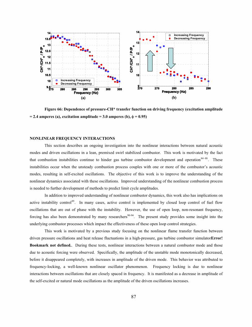
(a) (b)
275 280 285 290 295 300 3059.5
10
10.5
11
11.5
12
12.5
13
13.5
14
Frequency (Hz)
CH
* ′/C
H* o /
P ′/P
o
Increasing FrequencyDecreasing Frequency
270 275 280 285 2909
10
11
12
13
14
Frequency (Hz)
CH
* ′/C
H* o /
P ′/P
o
Increasing FrequencyDecreasing Frequency
(a) (b)
275 280 285 290 295 300 3059.5
10
10.5
11
11.5
12
12.5
13
13.5
14
Frequency (Hz)
CH
* ′/C
H* o /
P ′/P
o
Increasing FrequencyDecreasing Frequency
270 275 280 285 2909
10
11
12
13
14
Frequency (Hz)
CH
* ′/C
H* o /
P ′/P
o
Increasing FrequencyDecreasing Frequency
(a) (b)
275 280 285 290 295 300 3059.5
10
10.5
11
11.5
12
12.5
13
13.5
14
Frequency (Hz)
CH
* ′/C
H* o /
P ′/P
o
Increasing FrequencyDecreasing Frequency
270 275 280 285 2909
10
11
12
13
14
Frequency (Hz)
CH
* ′/C
H* o /
P ′/P
o
Increasing FrequencyDecreasing Frequency
Figure 66: Dependence of pressure-CH* transfer function on driving frequency (excitation amplitude
= 2.4 amperes (a), excitation amplitude = 3.0 amperes (b), φ = 0.95)
NONLINEAR FREQUENCY INTERACTIONS
This section describes an ongoing investigation into the nonlinear interactions between natural acoustic
modes and driven oscillations in a lean, premixed swirl stabilized combustor. This work is motivated by the fact
that combustion instabilities continue to hinder gas turbine combustor development and operation84-88. These
instabilities occur when the unsteady combustion process couples with one or more of the combustor’s acoustic
modes, resulting in self-excited oscillations. The objective of this work is to improve the understanding of the
nonlinear dynamics associated with these oscillations. Improved understanding of the nonlinear combustion process
is needed to further development of methods to predict limit cycle amplitudes.
In addition to improved understanding of nonlinear combustor dynamics, this work also has implications on
active instability control89. In many cases, active control is implemented by closed loop control of fuel flow
oscillations that are out of phase with the instability. However, the use of open loop, non-resonant frequency,
forcing has also been demonstrated by many researchers90-94. The present study provides some insight into the
underlying combustor processes which impact the effectiveness of these open loop control strategies.
This work is motivated by a previous study focusing on the nonlinear flame transfer function between
driven pressure oscillations and heat release fluctuations in a high-pressure, gas turbine combustor simulatorError!
Bookmark not defined.. During these tests, nonlinear interactions between a natural combustor mode and those
due to acoustic forcing were observed. Specifically, the amplitude of the unstable mode monotonically decreased,
before it disappeared completely, with increases in amplitude of the driven mode. This behavior was attributed to
frequency-locking, a well-known nonlinear oscillator phenomenon. Frequency locking is due to nonlinear
interactions between oscillations that are closely spaced in frequency. It is manifested as a decrease in amplitude of
the self-excited or natural mode oscillations as the amplitude of the driven oscillations increases.
87
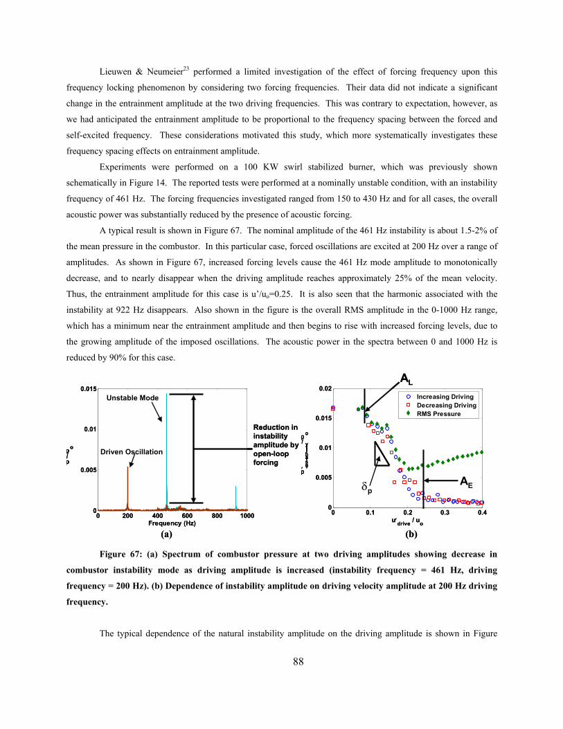
Lieuwen & Neumeier23 performed a limited investigation of the effect of forcing frequency upon this
frequency locking phenomenon by considering two forcing frequencies. Their data did not indicate a significant
change in the entrainment amplitude at the two driving frequencies. This was contrary to expectation, however, as
we had anticipated the entrainment amplitude to be proportional to the frequency spacing between the forced and
self-excited frequency. These considerations motivated this study, which more systematically investigates these
frequency spacing effects on entrainment amplitude.
Experiments were performed on a 100 KW swirl stabilized burner, which was previously shown
schematically in Figure 14. The reported tests were performed at a nominally unstable condition, with an instability
frequency of 461 Hz. The forcing frequencies investigated ranged from 150 to 430 Hz and for all cases, the overall
acoustic power was substantially reduced by the presence of acoustic forcing.
A typical result is shown in Figure 67. The nominal amplitude of the 461 Hz instability is about 1.5-2% of
the mean pressure in the combustor. In this particular case, forced oscillations are excited at 200 Hz over a range of
amplitudes. As shown in Figure 67, increased forcing levels cause the 461 Hz mode amplitude to monotonically
decrease, and to nearly disappear when the driving amplitude reaches approximately 25% of the mean velocity.
Thus, the entrainment amplitude for this case is u’/uo=0.25. It is also seen that the harmonic associated with the
instability at 922 Hz disappears. Also shown in the figure is the overall RMS amplitude in the 0-1000 Hz range,
which has a minimum near the entrainment amplitude and then begins to rise with increased forcing levels, due to
the growing amplitude of the imposed oscillations. The acoustic power in the spectra between 0 and 1000 Hz is
reduced by 90% for this case.
0 200 400 600 800 10000
0.005
0.01
0.015
Frequency (Hz)
p′ / po
0 0.1 0.2 0.3 0.40
0.005
0.01
0.015
0.02
u′drive / uo
p′instability /
po
Increasing DrivingDecreasing DrivingRMS Pressure
Driven Oscillation
Unstable Mode
(a)
Reduction in instability amplitude by open-loop forcing
(b)
AE
AL
δp
0 200 400 600 800 10000
0.005
0.01
0.015
Frequency (Hz)
p′ / po
0 0.1 0.2 0.3 0.40
0.005
0.01
0.015
0.02
u′drive / uo
p′instability /
po
Increasing DrivingDecreasing DrivingRMS Pressure
Driven Oscillation
Unstable Mode
(a)
Reduction in instability amplitude by open-loop forcing
(b)
AE
AL
δp
Figure 67: (a) Spectrum of combustor pressure at two driving amplitudes showing decrease in
combustor instability mode as driving amplitude is increased (instability frequency = 461 Hz, driving
frequency = 200 Hz). (b) Dependence of instability amplitude on driving velocity amplitude at 200 Hz driving
frequency.
The typical dependence of the natural instability amplitude on the driving amplitude is shown in Figure
88
67(b). At the highest driving amplitudes, the instability has essentially disappeared at the cost of the increase in
amplitude of the driven pressure. There are several basic features of the instability amplitude dependence upon
driving amplitude that can be discerned from Figure 67(b). First, the instability amplitude is independent of the
forcing amplitude for some amplitude range before decreasing; we have referred to the driving amplitude at which
this decrease begins as AL. Second, the instability amplitude decreases with some slope, δp, for further driving
amplitude increases. Third, the instability amplitude essentially goes to zero, or to near zero values above some
driving amplitude, referred to here as the entrainment amplitude, Ae. For example, in Figure 67(b) the entrainment
amplitude is ~25% of the mean velocity at the premixer exit. Finally, the dependence of the unstable mode
amplitude upon the driving amplitude exhibits some hysteresis. In this study, hysteresis occurred at only at select
frequencies in the 150-430 range we have tested so far at this instability condition. No significant trend was found
that was dependent on driving frequency. This hysteresis behavior is shown in Figure 68. Typical hysteresis levels
are found to be between 3-5% of the mean velocity value.
These characteristics depend significantly upon driving frequency. We consider first the entrainment
amplitude dependence upon driving frequency, which is plotted in Figure 69(a). The entrainment amplitude, AE,
grows as the forcing frequency is moved away from the instability frequency of 461 Hz, except very close to the
instability (fdrive = 400-430 Hz). The trend in Figure 69 was expected although we do not have any specific theory
our intuition was based upon. Figure 69 also reinforces the fact that the velocity oscillation amplitude in unstable
combustors is a major controlling factor which affects the nonlinear combustion process. It should be noted that a
different trend is observed if the perturbation pressure§ (see Figure 69b), rather than velocity were used to quantify
the forcing amplitude. This is due to the frequency dependence of the pressure-velocity relation. This result
explains the confusion over this issue raised in our prior study, which used the perturbation pressure as a measure of
disturbance amplitude.
§ In this combustor, the entrainment pressure amplitude increases monotonically with decreasing frequency up to
about 230 Hz. It then decreases for lower frequencies.
89
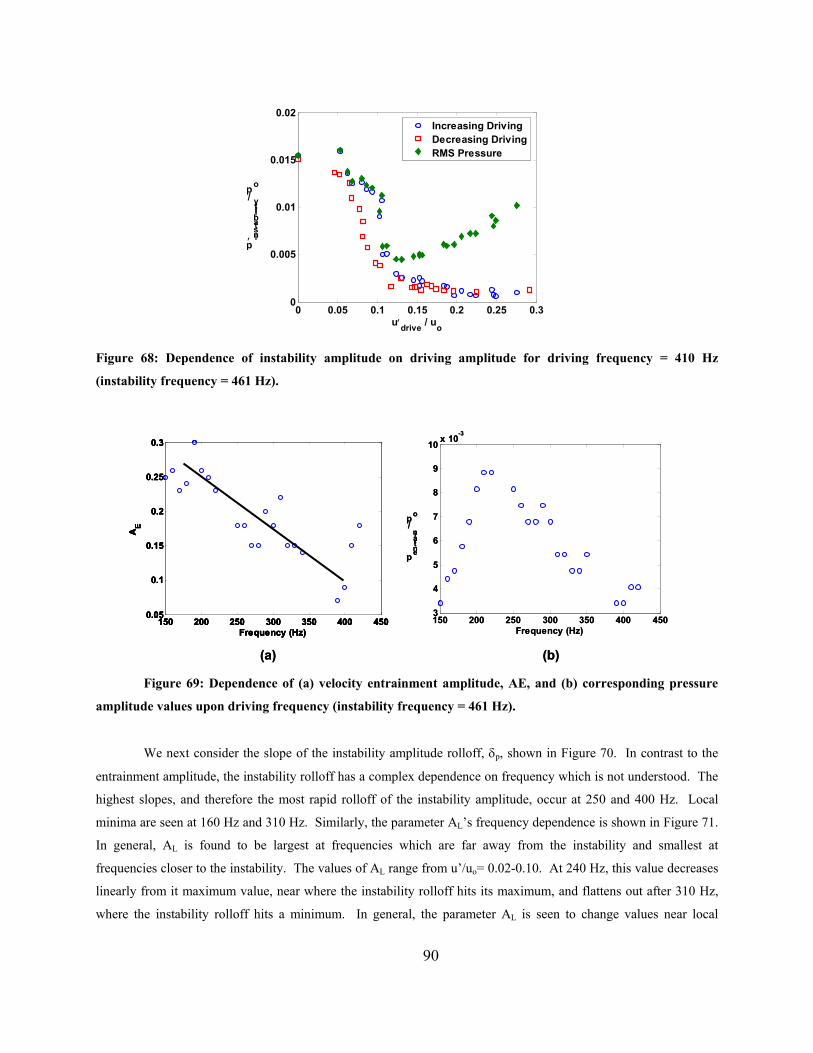
0 0.05 0.1 0.15 0.2 0.25 0.30
0.005
0.01
0.015
0.02
u′drive / uo
p′instability /
po
Increasing DrivingDecreasing DrivingRMS Pressure
Figure 68: Dependence of instability amplitude on driving amplitude for driving frequency = 410 Hz
(instability frequency = 461 Hz).
(a) (b)
150 200 250 300 350 400 4500.05
0.1
0.15
0.2
0.25
0.3
Frequency (Hz)
AE
150 200 250 300 350 400 4500.05
0.1
0.15
0.2
0.25
0.3
Frequency (Hz)
AE
150 200 250 300 350 400 4503
4
5
6
7
8
9
10 x 10-3
Frequency (Hz)
p entrain /
po
(a) (b)
150 200 250 300 350 400 4500.05
0.1
0.15
0.2
0.25
0.3
Frequency (Hz)
AE
150 200 250 300 350 400 4500.05
0.1
0.15
0.2
0.25
0.3
Frequency (Hz)
AE
150 200 250 300 350 400 4503
4
5
6
7
8
9
10 x 10-3
Frequency (Hz)
p entrain /
po
Figure 69: Dependence of (a) velocity entrainment amplitude, AE, and (b) corresponding pressure
amplitude values upon driving frequency (instability frequency = 461 Hz).
We next consider the slope of the instability amplitude rolloff, δp, shown in Figure 70. In contrast to the
entrainment amplitude, the instability rolloff has a complex dependence on frequency which is not understood. The
highest slopes, and therefore the most rapid rolloff of the instability amplitude, occur at 250 and 400 Hz. Local
minima are seen at 160 Hz and 310 Hz. Similarly, the parameter AL’s frequency dependence is shown in Figure 71.
In general, AL is found to be largest at frequencies which are far away from the instability and smallest at
frequencies closer to the instability. The values of AL range from u’/uo= 0.02-0.10. At 240 Hz, this value decreases
linearly from it maximum value, near where the instability rolloff hits its maximum, and flattens out after 310 Hz,
where the instability rolloff hits a minimum. In general, the parameter AL is seen to change values near local
90
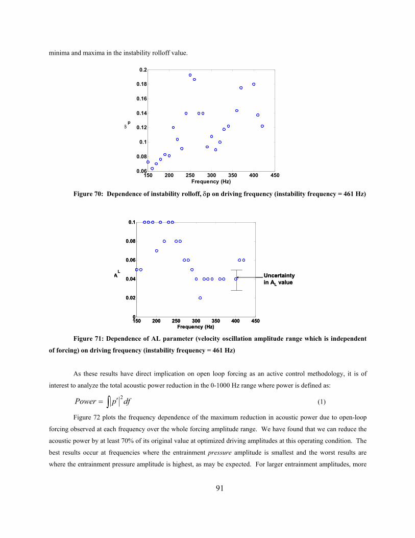
minima and maxima in the instability rolloff value.
150 200 250 300 350 400 4500.06
0.08
0.1
0.12
0.14
0.16
0.18
0.2
Frequency (Hz)
δp
Figure 70: Dependence of instability rolloff, δp on driving frequency (instability frequency = 461 Hz)
150 200 250 300 350 400 4500
0.02
0.04
0.06
0.08
0.1
Frequency (Hz)
AL
Uncertainty in AL value
150 200 250 300 350 400 4500
0.02
0.04
0.06
0.08
0.1
Frequency (Hz)
AL
Uncertainty in AL value
Figure 71: Dependence of AL parameter (velocity oscillation amplitude range which is independent
of forcing) on driving frequency (instability frequency = 461 Hz)
As these results have direct implication on open loop forcing as an active control methodology, it is of
interest to analyze the total acoustic power reduction in the 0-1000 Hz range where power is defined as:
dfpPower ∫ ′= 2 (1)
Figure 72 plots the frequency dependence of the maximum reduction in acoustic power due to open-loop
forcing observed at each frequency over the whole forcing amplitude range. We have found that we can reduce the
acoustic power by at least 70% of its original value at optimized driving amplitudes at this operating condition. The
best results occur at frequencies where the entrainment pressure amplitude is smallest and the worst results are
where the entrainment pressure amplitude is highest, as may be expected. For larger entrainment amplitudes, more
91
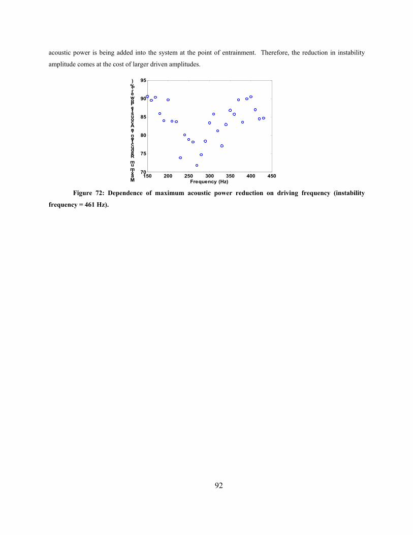
acoustic power is being added into the system at the point of entrainment. Therefore, the reduction in instability
amplitude comes at the cost of larger driven amplitudes.
150 200 250 300 350 400 45070
75
80
85
90
95
Frequency (Hz)Maximum Reduction in Acoustic Power (%)
Figure 72: Dependence of maximum acoustic power reduction on driving frequency (instability
frequency = 461 Hz).
92
9. Active Control of Combustion Instabilities This note describes an experimental investigation of active control of instabilities in a high pressure, liquid
fueled combustor. Active control has been widely demonstrated as a technically viable method for suppressing
combustion instabilities (e.g., see Refs. [95, 96,97]). For example, it has been shown that instabilities can be
suppressed by measuring the pressure or heat release in the combustor, suitably phase shifting and amplifying the
measured signal, then driving a secondary fuel injector with this signal. While significant progress has been made, a
number of problems are still in need of investigation. Active controllers are often found to work well at certain
operating conditions, while their effectiveness is significantly reduced at others. Results in the literature quantifying
the degree of suppression of the instability amplitude vary substantially, from factors of under 2 to over 50.
Experiments have shown that the same methodology performs very differently on different combustors and at
different operating conditions. Thus, although at this point it is well established that some degree of suppression of
combustion instabilities is possible, more research is needed to understand the dynamics of actively controlled
combustors and the factors that limit control effectiveness.
A variety of factors determine the impact of an active control system upon an instability. First, the
uncontrolled combustor dynamics play a significant role on the effect active control has upon the oscillations.
Control effectiveness will clearly depend upon such issues as instability amplitude, instability frequency and
background noise levels. In addition, nonlinear characteristics of the combustor, such as hysteresis and saturation,
play important roles in control effectiveness.
Next, the issues of observability and controllability are significant; i.e., the extent to which the state of the
system can be sensed and affected by actuation, respectively. Observability does not appear to be a significant issue
limiting control effectiveness, unless, for example, a pressure sensor is located in a node. Controllability issues are
more significant due to the challenges of actuating coherent fuel pulses at high frequencies. In many cases, liquid
fuel is actuated using on-off, pulse-width modulations which causes spectral broadening of the excited heat release
oscillations about the carrier wave frequency. This broadening is partially responsible for the peak splitting
phenomenon discussed by Cohen and Banaszuk [1]. Cohen and Banaszuk [1] and Lee and Santavicca [24] have
also emphasized the importance of fuel placement and/or mixedness upon control effectiveness.
Turning to the controller itself, the poorly understood nonlinear and stochastic nature of crucial combustor
processes renders classical model based approaches difficult for implementation on actual hardware. Prior
experimental controllers have either filtered the pressure/ chemiluminescence signal about the instability frequency
(which must be known a priori) or used observers to extract the amplitude and frequency of the instability. The
optimal control phase is typically determined using either off-line testing or adaptive schemes.
Probably one of the most significant factors determining the effectiveness of the combined controller-
actuation system is the overall controller time delay. As might be expected, several studies have shown that the
combined effects of background noise and time delays substantially impair control effectiveness. For example, it
has been observed that the combustor appears to “run away” from the control when sufficient control actuation is
93
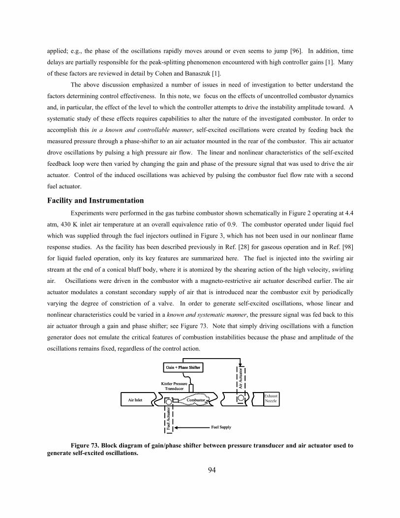
applied; e.g., the phase of the oscillations rapidly moves around or even seems to jump [96]. In addition, time
delays are partially responsible for the peak-splitting phenomenon encountered with high controller gains [1]. Many
of these factors are reviewed in detail by Cohen and Banaszuk [1].
The above discussion emphasized a number of issues in need of investigation to better understand the
factors determining control effectiveness. In this note, we focus on the effects of uncontrolled combustor dynamics
and, in particular, the effect of the level to which the controller attempts to drive the instability amplitude toward. A
systematic study of these effects requires capabilities to alter the nature of the investigated combustor. In order to
accomplish this in a known and controllable manner, self-excited oscillations were created by feeding back the
measured pressure through a phase-shifter to an air actuator mounted in the rear of the combustor. This air actuator
drove oscillations by pulsing a high pressure air flow. The linear and nonlinear characteristics of the self-excited
feedback loop were then varied by changing the gain and phase of the pressure signal that was used to drive the air
actuator. Control of the induced oscillations was achieved by pulsing the combustor fuel flow rate with a second
fuel actuator.
Facility and Instrumentation Experiments were performed in the gas turbine combustor shown schematically in Figure 2 operating at 4.4
atm, 430 K inlet air temperature at an overall equivalence ratio of 0.9. The combustor operated under liquid fuel
which was supplied through the fuel injectors outlined in Figure 3, which has not been used in our nonlinear flame
response studies. As the facility has been described previously in Ref. [28] for gaseous operation and in Ref. [98]
for liquid fueled operation, only its key features are summarized here. The fuel is injected into the swirling air
stream at the end of a conical bluff body, where it is atomized by the shearing action of the high velocity, swirling
air. Oscillations were driven in the combustor with a magneto-restrictive air actuator described earlier. The air
actuator modulates a constant secondary supply of air that is introduced near the combustor exit by periodically
varying the degree of constriction of a valve. In order to generate self-excited oscillations, whose linear and
nonlinear characteristics could be varied in a known and systematic manner, the pressure signal was fed back to this
air actuator through a gain and phase shifter; see Figure 73. Note that simply driving oscillations with a function
generator does not emulate the critical features of combustion instabilities because the phase and amplitude of the
oscillations remains fixed, regardless of the control action.
Air
Act
uato
r
Fuel SupplyFuel
Act
uato
r
CombustorExhaust NozzleAir Inlet
Kistler Pressure Transducer
Gain + Phase Shifter
Air
Act
uato
r
Fuel SupplyFuel
Act
uato
r
CombustorExhaust NozzleExhaust NozzleExhaust NozzleAir Inlet
Kistler Pressure Transducer
Gain + Phase ShifterGain + Phase Shifter
Figure 73. Block diagram of gain/phase shifter between pressure transducer and air actuator used to generate self-excited oscillations.
94
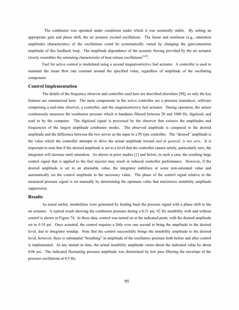
The combustor was operated under conditions under which it was nominally stable. By setting an
appropriate gain and phase shift, the air actuator excited oscillations. The linear and nonlinear (e.g., saturation
amplitude) characteristics of the oscillations could be systematically varied by changing the gain/saturation
amplitude of this feedback loop. The amplitude dependence of the acoustic forcing provided by the air actuator
closely resembles the saturating characteristic of heat release oscillations16,99.
Fuel for active control is modulated using a second magnetostrictive fuel actuator. A controller is used to
maintain the mean flow rate constant around the specified value, regardless of amplitude of the oscillating
component.
Control Implementation The details of the frequency observer and controller used here are described elsewhere [98], so only the key
features are summarized here. The main components in the active controller are a pressure transducer, software
comprising a real-time observer, a controller, and the magnetostrictive fuel actuator. During operation, the sensor
continuously measures the combustor pressure which is bandpass filtered between 20 and 1000 Hz, digitized, and
read in by the computer. The digitized signal is processed by the observer that extracts the amplitudes and
frequencies of the largest amplitude combustor modes. The observed amplitude is compared to the desired
amplitude and the difference between the two serves as the input to a PI type controller. The “desired” amplitude is
the value which the controller attempts to drive the actual amplitude toward and in general, is not zero. It is
important to note that if the desired amplitude is set to a level that the controller cannot satisfy, particularly zero, the
integrator will increase until saturation. As shown in prior studies [1] and below, in such a case, the resulting large
control signal that is applied to the fuel injector may result in reduced controller performance. However, if the
desired amplitude is set to an attainable value, the integrator stabilizes at some non-saturated value and
automatically set the control amplitude to the necessary value. The phase of the control signal relative to the
measured pressure signal is set manually by determining the optimum value that maximizes instability amplitude
suppression.
Results As noted earlier, instabilities were generated by feeding back the pressure signal with a phase shift to the
air actuator. A typical result showing the combustor pressure during a 0.31 psi, 92 Hz instability with and without
control is shown in Figure 74. In these data, control was turned on at the indicated point, with the desired amplitude
set to 0.18 psi. Once actuated, the control requires a little over one second to bring the amplitude to the desired
level, due to integrator windup. Note that the control successfully brings the instability amplitude to the desired
level; however, there is substantial “breathing” in amplitude of the oscillatory pressure both before and after control
is implemented. At any instant in time, the actual instability amplitude varies about the indicated value by about
0.06 psi. The indicated fluctuating pressure amplitude was determined by low pass filtering the envelope of the
pressure oscillations at 0.5 Hz.
95
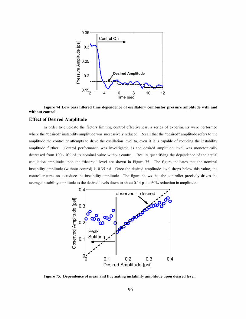
2 4 6 8 10 120.15
0.2
0.25
0.3
0.35
Time [sec]
Pre
ssur
e Am
plitu
de [p
si]
ObservedDesiredControl On
Desired Amplitude
Figure 74 Low pass filtered time dependence of oscillatory combustor pressure amplitude with and without control.
Effect of Desired Amplitude In order to elucidate the factors limiting control effectiveness, a series of experiments were performed
where the “desired” instability amplitude was successively reduced. Recall that the “desired” amplitude refers to the
amplitude the controller attempts to drive the oscillation level to, even if it is capable of reducing the instability
amplitude further. Control performance was investigated as the desired amplitude level was monotonically
decreased from 100 - 0% of its nominal value without control. Results quantifying the dependence of the actual
oscillation amplitude upon the “desired” level are shown in Figure 75. The figure indicates that the nominal
instability amplitude (without control) is 0.35 psi. Once the desired amplitude level drops below this value, the
controller turns on to reduce the instability amplitude. The figure shows that the controller precisely drives the
average instability amplitude to the desired levels down to about 0.14 psi, a 60% reduction in amplitude.
0 0.1 0.2 0.3 0.40
0.1
0.2
0.3
0.4
Desired Amplitude [psi]
Obs
erve
d A
mpl
itude
[psi
]
observed = desired
Peak Splitting
Figure 75. Dependence of mean and fluctuating instability amplitude upon desired level.
96
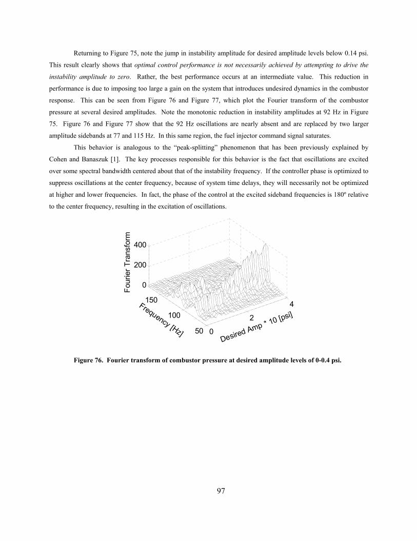
Returning to Figure 75, note the jump in instability amplitude for desired amplitude levels below 0.14 psi.
This result clearly shows that optimal control performance is not necessarily achieved by attempting to drive the
instability amplitude to zero. Rather, the best performance occurs at an intermediate value. This reduction in
performance is due to imposing too large a gain on the system that introduces undesired dynamics in the combustor
response. This can be seen from Figure 76 and Figure 77, which plot the Fourier transform of the combustor
pressure at several desired amplitudes. Note the monotonic reduction in instability amplitudes at 92 Hz in Figure
75. Figure 76 and Figure 77 show that the 92 Hz oscillations are nearly absent and are replaced by two larger
amplitude sidebands at 77 and 115 Hz. In this same region, the fuel injector command signal saturates.
This behavior is analogous to the “peak-splitting” phenomenon that has been previously explained by
Cohen and Banaszuk [1]. The key processes responsible for this behavior is the fact that oscillations are excited
over some spectral bandwidth centered about that of the instability frequency. If the controller phase is optimized to
suppress oscillations at the center frequency, because of system time delays, they will necessarily not be optimized
at higher and lower frequencies. In fact, the phase of the control at the excited sideband frequencies is 180º relative
to the center frequency, resulting in the excitation of oscillations.
50
100
150
0
2
4
0
200
400
Desired Amp * 10 [psi]Frequency [Hz]
Four
ier T
rans
form
Figure 76. Fourier transform of combustor pressure at desired amplitude levels of 0-0.4 psi.
97
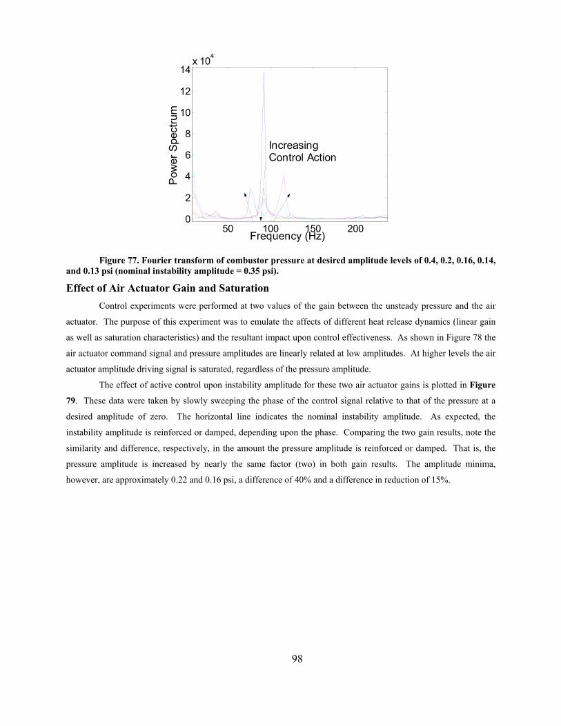
50 100 150 2000
2
4
6
8
10
12
14
Frequency (Hz)
Pow
er S
pect
rum
Increasing Control Action
x 104
Figure 77. Fourier transform of combustor pressure at desired amplitude levels of 0.4, 0.2, 0.16, 0.14, and 0.13 psi (nominal instability amplitude = 0.35 psi).
Effect of Air Actuator Gain and Saturation Control experiments were performed at two values of the gain between the unsteady pressure and the air
actuator. The purpose of this experiment was to emulate the affects of different heat release dynamics (linear gain
as well as saturation characteristics) and the resultant impact upon control effectiveness. As shown in Figure 78 the
air actuator command signal and pressure amplitudes are linearly related at low amplitudes. At higher levels the air
actuator amplitude driving signal is saturated, regardless of the pressure amplitude.
The effect of active control upon instability amplitude for these two air actuator gains is plotted in Figure
79. These data were taken by slowly sweeping the phase of the control signal relative to that of the pressure at a
desired amplitude of zero. The horizontal line indicates the nominal instability amplitude. As expected, the
instability amplitude is reinforced or damped, depending upon the phase. Comparing the two gain results, note the
similarity and difference, respectively, in the amount the pressure amplitude is reinforced or damped. That is, the
pressure amplitude is increased by nearly the same factor (two) in both gain results. The amplitude minima,
however, are approximately 0.22 and 0.16 psi, a difference of 40% and a difference in reduction of 15%.
98
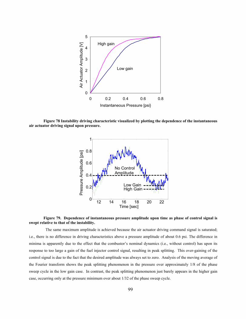
0
1
2
3
4
5
0 0.2 0.4 0.6 0.8
Instantaneous Pressure [psi}
Air A
ctua
tor A
mpl
itude
[V]
Low gain
High gain
Figure 78 Instability driving characteristic visualized by plotting the dependence of the instantaneous air actuator driving signal upon pressure.
12 14 16 18 20 220
0.2
0.4
0.6
0.8
1
Time [sec]
Pre
ssur
e A
mpl
itude
[psi
]
High Gain Low Gain
No Control Amplitude
Figure 79. Dependence of instantaneous pressure amplitude upon time as phase of control signal is swept relative to that of the instability.
The same maximum amplitude is achieved because the air actuator driving command signal is saturated;
i.e., there is no difference in driving characteristics above a pressure amplitude of about 0.6 psi. The difference in
minima is apparently due to the effect that the combustor’s nominal dynamics (i.e., without control) has upon its
response to too large a gain of the fuel injector control signal, resulting in peak splitting. This over-gaining of the
control signal is due to the fact that the desired amplitude was always set to zero. Analysis of the moving average of
the Fourier transform shows the peak splitting phenomenon in the pressure over approximately 1/8 of the phase
sweep cycle in the low gain case. In contrast, the peak splitting phenomenon just barely appears in the higher gain
case, occurring only at the pressure minimum over about 1/32 of the phase sweep cycle.
99
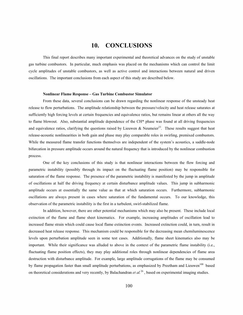
10. CONCLUSIONS
This final report describes many important experimental and theoretical advances on the study of unstable
gas turbine combustors. In particular, much emphasis was placed on the mechanisms which can control the limit
cycle amplitudes of unstable combustors, as well as active control and interactions between natural and driven
oscillations. The important conclusions from each aspect of this study are described below.
Nonlinear Flame Response – Gas Turbine Combustor Simulator
From these data, several conclusions can be drawn regarding the nonlinear response of the unsteady heat
release to flow perturbations. The amplitude relationship between the pressure/velocity and heat release saturates at
sufficiently high forcing levels at certain frequencies and equivalence ratios, but remains linear at others all the way
to flame blowout. Also, substantial amplitude dependence of the CH* phase was found at all driving frequencies
and equivalence ratios, clarifying the questions raised by Lieuwen & Neumeier23. These results suggest that heat
release-acoustic nonlinearities in both gain and phase may play comparable roles in swirling, premixed combustors.
While the measured flame transfer functions themselves are independent of the system’s acoustics, a saddle-node
bifurcation in pressure amplitude occurs around the natural frequency that is introduced by the nonlinear combustion
process.
One of the key conclusions of this study is that nonlinear interactions between the flow forcing and
parametric instability (possibly through its impact on the fluctuating flame position) may be responsible for
saturation of the flame response. The presence of the parametric instability is manifested by the jump in amplitude
of oscillations at half the driving frequency at certain disturbance amplitude values. This jump in subharmonic
amplitude occurs at essentially the same value as that at which saturation occurs. Furthermore, subharmonic
oscillations are always present in cases where saturation of the fundamental occurs. To our knowledge, this
observation of the parametric instability is the first in a turbulent, swirl-stabilized flame.
In addition, however, there are other potential mechanisms which may also be present. These include local
extinction of the flame and flame sheet kinematics. For example, increasing amplitudes of oscillation lead to
increased flame strain which could cause local flame extinction events. Increased extinction could, in turn, result in
decreased heat release response. This mechanism could be responsible for the decreasing mean chemiluminescence
levels upon perturbation amplitude seen in some test cases. Additionally, flame sheet kinematics also may be
important. While their significance was alluded to above in the context of the parametric flame instability (i.e.,
fluctuating flame position effects), they may play additional roles through nonlinear dependencies of flame area
destruction with disturbance amplitude. For example, large amplitude corrugations of the flame may be consumed
by flame propagation faster than small amplitude perturbations, as emphasized by Preetham and Lieuwen100 based
on theoretical considerations and very recently, by Balachandran et al.26 , based on experimental imaging studies.
100
While it is not possible to conclusively determine the relative roles of all potential mechanisms of
nonlinearity, we can eliminate some mechanisms which have been suggested as potentially significant:
Global” Extinction – This is the mechanism proposed by Dowling16 and Poinsot et al.19 which follows
from the simple observation that the instantaneous heat release cannot go negative, thus limiting the
chemiluminescence fluctuations to 100% of the mean value. Our data indicate saturation at substantially lower
amplitudes, however, implying that this mechanism is not significant in this combustor.
Chemical Kinetics – Reaction rates depend upon pressure and temperature in a nonlinear manner. These
nonlinearities will apparently become significant when the fluctuating pressure and temperature achieve amplitudes
on the order of their mean values. This mechanism does not appear likely here, however, as nonlinearity occurs at
p’/po values of ~2%.
Equivalence ratio oscillations – The nonlinear dependence of the equivalence ratio amplitude and heat
release response discussed by Peracchio & Proscia17 and Lieuwen15 is not important here, as the fuel/air mixture had
a constant composition. As such, though we cannot comment on the magnitude of these types of nonlinearities in
situations where they are present, the data presented here indicate that other flame processes also cause
nonlinearities in flame response.
Flame holding – The many data indicating a linear CH* response all the way to blowoff indicate that
nonlinearities due to marginal flame holding are probably not important
Nonlinear Flame Response – Atmospheric Burner
From the results presented, we can make the following conclusions. First, substantial nonlinearities in the
flame response to forced velocity oscillations have been shown. The phase between the flow oscillation and heat
release is also seen to have substantial amplitude dependence. Various mechanisms appear to be important in
different frequency and flowrate regimes. For instance, at low flow rates, the saturation amplitude of CH* can vary
greatly with driving frequency and range from 25-100% of the mean value. In contrast, for higher flow rates, it is
observed that the nonlinear amplitude of CH* is roughly independent of driving frequency. In addition, the shape of
the transfer function can change markedly for different driving frequencies and flow rates. Therefore, there are a
variety of behaviors which are present in a single combustor. Thus, one single theory is not adequate to describe the
nonlinear dynamics of a forced or unstable combustor.
OH PLIF imaging of the flame was performed at two frequencies where two mechanisms potentially
controlled the saturation amplitude of the global heat release from the flame. Two phenomena, vortex rollup and
flame liftoff, are found to be the likely mechanisms which govern saturation of the flame transfer function from
these images. The latter mechanism visibly changes the flame structure when comparing these results with line-of-
sight images. Both mechanisms act to reduce the flame area.
No sub-harmonic flame response was observed in any of these studies, as opposed to the earlier study in the
combustor simulator as mentioned above. This result is not understood, as it is well known that parametric flame
instabilities occur at high forcing amplitudes, resulting in a subharmonic response. Future work will attempt to
101
reconcile these differing observations
Theoretical Nonlinear Flame Response
One of the key points made here is that the linear and nonlinear characteristics of the flame dynamics are
controlled by the interaction between flame disturbances due to boundaries and flow non-uniformities. A
constructive superposition of the two flame disturbance contributions can cause the flame to act as an “amplifier” at
certain frequencies whereas a destructive superposition can cause the flame response to be identically zero. The
theory also captures the effect of flame stretch and shows that it is responsible for the experimentally observed
phenomenon of “filtering”.
In the nonlinear regime, the flame response is critically dependent on whether the solution lies in a region
of constructive or destructive interference of the flame disturbances. In regions of constructive interference, the
nonlinear flame transfer function gain is always less than its linear value whereas in regions of destructive
interference the nonlinear transfer function may exceed its linear value. These characteristics can cause the same
combustor to exhibit sub-or supercritical type of bifurcation depending on the operating condition. The analysis
shows that nonlinearity is enhanced and that there is a greater tendency for the nonlinear transfer function to have an
inflection point when the phase speed of the disturbances is less than the mean flow speed. Moreover, the average
flame length decreases with increasing perturbation amplitude for most conditions which is consistent with the
available experimental data.
Several additional studies are motivated by this work. First is an analysis of the nonlinear flame response in
cases where the flame is being simultaneously disturbed by deterministic harmonic fluctuations as well as random
fluctuations. The latter fluctuations simulate the impact of background turbulent fluctuations. As such, the analysis
would allow for a rudimentary comparison of the nonlinear dynamics of laminar and turbulent flames. Second there
is a need to couple the flow field and flame dynamics so that the effect of gas expansion can be captured. This would
introduce a new parameter into the results, the ratio Tb/Tu.
Nonlinear Interactions in Unstable Combustors
These results have implications of the type of bifurcations which may be observed in unstable combustors.
This study clarifies a number of issues related to the nonlinear interactions between driven and natural unstable
combustor modes but also raises new questions. It has been shown that the entrainment velocity amplitude
monotonically grows with driving-instability frequency separation. We have found that the instability rolloff and
velocity oscillation range which is independent of forcing amplitude both have complex dependencies on driving
frequency. Changes in the parameter, AL, are seen to accompany local minima and maxima in instability rolloff.
Further work is being performed to analyze the effect on these parameters of driving frequencies greater than the
instability frequency.
In addition, open loop forcing of the combustor, at frequencies different from the instability frequency, was
102
found to significantly reduce the acoustic power in the 0-1000 Hz range by as much as 90%. The performance of
this open loop control scheme is dependent on the entrainment amplitude. The best results were obtained for
frequencies which had the lowest entrainment pressure amplitudes, as might be expected.
The generality of this methodology is an open question, however, as we found some operating conditions
where entrainment did not occur in the same fashion and the instability amplitude is marginally reduced. For
example, in one situation, the addition of forcing caused a shift in instability frequency to a value 40 Hz higher than
its unforced value (from 510 Hz to 550 Hz). For driving frequencies whose harmonics do not fall around this new
frequency, this value is relatively constant. The acoustic power in the 0-1000 Hz range is only slight reduced
(~20%) before increasing rapidly, unlike the conditions presented in this paper. An investigation on this behavior is
also ongoing.
The theoretical study has further highlighted the importance of the interactions between the contributions
from flame disturbances due to boundaries and flow non-uniformities. The present investigation extends the
analytical solutions for the flame response from the linear to the non-linear regime.
Active Control Studies of Unstable Combustors
A variety of factors determine the impact of an active control system upon an instability. First, the
uncontrolled combustor dynamics play a significant role on the effect active control has upon the oscillations.
Control effectiveness will clearly depend upon such issues as instability amplitude, instability frequency and
background noise levels. In addition, nonlinear characteristics of the combustor, such as hysteresis and saturation,
play important roles in control effectiveness.
.
103
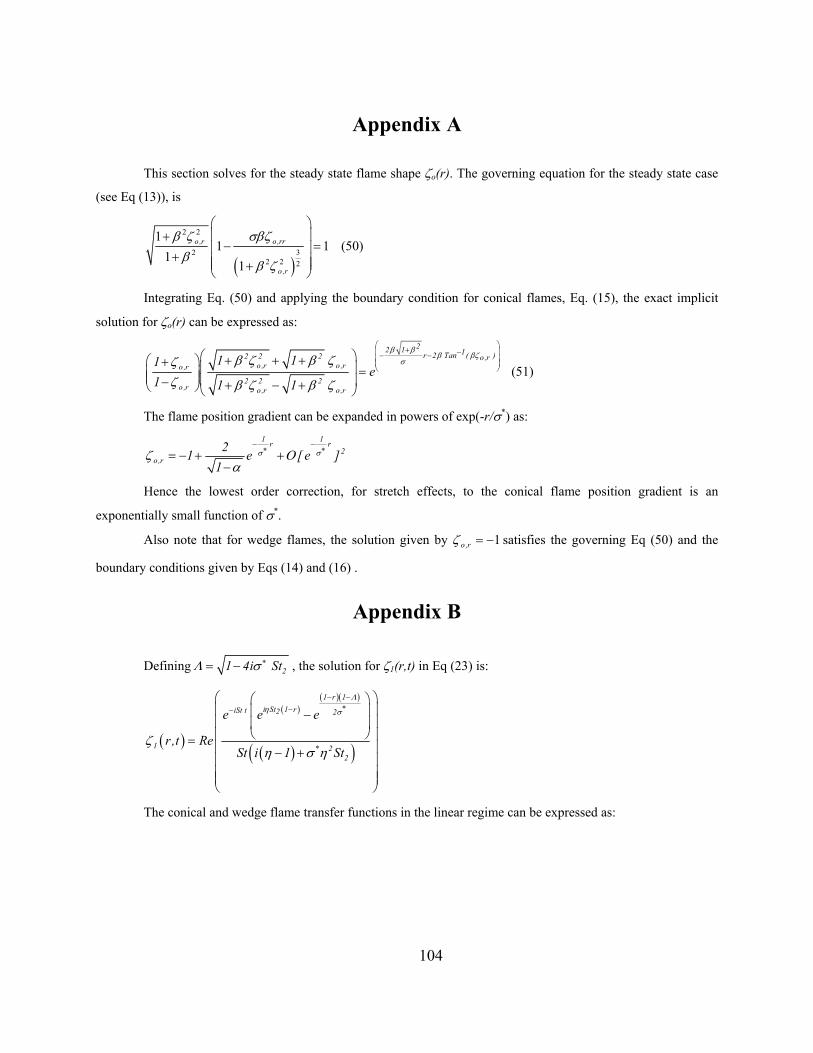
Appendix A
This section solves for the steady state flame shape ζo(r). The governing equation for the steady state case
(see Eq (13)), is
( )
2 2
2 32 2 2
11 1
11
o,r o,rr
o,r
β ζ σβζβ
β ζ
+
− = + +
(50)
Integrating Eq. (50) and applying the boundary condition for conical flames, Eq. (15), the exact implicit
solution for ζo(r) can be expressed as:
22 1 1r 2 Tan ( )2 2 2 o,ro,r o,ro,r
2 2 2o,r o,r o,r
1 11e
1 1 1
β ββ βζ
σβ ζ β ζζζ β ζ β ζ
+ −− −
+ + + + = − + − + (51)
The flame position gradient can be expanded in powers of exp(-r/σ*) as: 1 1r r
2o,r
21 e [ e1
σ σζ Οα
− −∗ ∗= − + +
−]
Hence the lowest order correction, for stretch effects, to the conical flame position gradient is an
exponentially small function of σ*.
Also note that for wedge flames, the solution given by 1o,rζ = − satisfies the governing Eq (50) and the
boundary conditions given by Eqs (14) and (16) .
Appendix B
Defining 21 4i StΛ σ ∗= − , the solution for ζ1(r,t) in Eq (23) is:
( )
( )( )( )
( )( )
1 r 1*i St 1 riSt t 2 2
1 * 22
e e e
r,t ReSt i 1 St
Λη σ
ζη σ η
− −
−− −
= − +
The conical and wedge flame transfer functions in the linear regime can be expressed as:
104
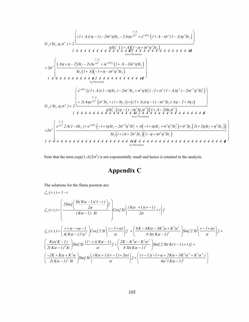
( )
( )( )
( ) ( )( )
1i St 22 2
2 2
c 2 2 22 2
Area Fluctuation
1i St2 2
2 2
2
( 1 )( 1 ) 2i St 2 e e 1 i (1 ) St
G ( St , , ) 2St 1 1 i St
2 St 2i e ie 1 2i St2
St 1 1 i
Λησ
Λησ
Λ η σ η Λη Λ σ Λ η
η ση Λ η σ η
Λη η Λ Λ σ ησ
Λ η
−∗∗ ∗
∗∗
−∗ ∗
∗
+ − − − + + − − =
+ − +
+ − − + + −+
+ − + −
1 4 4 4 4 4 4 4 4 4 4 4 4 4 442 4 4 4 4 4 4 4 4 4 4 4 4 4 443
( )22
S FluctuationL
Stσ η∗
1 4 4 4 4 4 4 4 4 4 4 44 2 4 4 4 4 4 4 4 4 4 4 443
( )
)( ( )( ) ( )
i St 2 2 2 3 322 2 2 2
1
22 2 2
w 2 2 22 2 2
Area Fluctuation
e ( 1 )(1 i St ) 2i St St ( 2 ( 1 ) ) 2i St
2i e St ( i St ) ( 1 )( 1 ) i St ( 2 3 )G ( St , , ) 2
St ( 1 ) i St 1 2iSt
η
Λ
σ
Λ η σ σ η σ Λ η σ η
Λη σ Λ η σ Λη ηη σ
η η η σ Λ σ
∗ ∗ ∗ ∗
−∗ ∗ ∗
∗∗ ∗
+ − − + − + − − + + + + + − − − + =
− − + −1 4 4 4 4 4 4 4 4 4 4 4 4 4 4 4 2
( ) (( )( ) ( )
)1
i St 2 2 2 2 2 22 22 2 2 2 2 2 2
22 2 2
S FluctuationL
e 2 (1 iSt ) e 1 i St 2 St 1 i St St St 2i 2 St St2
St i i 2 St 1 i St
Λησ Λ η σ η Λ η σ η σ η
σΛ σ η σ η
−∗ ∗ ∗ ∗
∗∗ ∗
− + − + − + − + + + + + + + + − +
4 4 4 4 4 4 4 4 4 4 4 4 4 4 4 4 43
1 4 4 4 4 4 4 4 4 4 4 4 4 4 4 4 4 4 4 4 4 4442 4 4 4 4 4 4 4 4 4 4 4 4 4 4 4 4 4 4 4 34 4 44
2η
Note that the term exp((1-Λ)/2σ*) is not exponentially small and hence is retained in the analysis.
Appendix C
The solutions for the flame position are:
o ( r ,t ) 1 rζ = −
1
St( K 1)(1 r )2Sin[ ]( K 1)( r 1)2( r ,t ) Cos[ St t ]
( K 1) St 2
αααζ
α α
− − + − = + −
2 2 2
2 2 2 3
2 2 2
3 3
r r 1 r 1 t 6K 4K 3K K r 1 t( r ,t ) Cos[ 2 St ] Sin[ 2 St ]4( K 1) 8 St( K 1)
K ( K 1) (1 r )( K 1) 2K K KSin[ St ] Sin[ 2 St( K( r 1) t )]2( K 1) St 8 St( K 1)
2K
α α α α α α αζα αα α α
α α α ααα α
+ − − − + − − + − + = + − −
− − − − −+ − + +
− −
−
+
2 2 2 2 3
3 2 2
K K ( K 1)( r 1) 2 t ( r 1)( 1 2K 3K K )Sin[ St ]2( K 1) St 4 ( K 1)
α α α α α α α ααα α
+ + + − + − − + + − + + − − α
105
2 2 2 2 3 3 3
3 4 3
2 2 2 2 4 2 2 2 2 2 3 3 2 3 3
5 4
( r 1)(1 )( 3 13K 4K 13K 3K 10K ) r 1 t( r ,t ) Cos[ St ]8( K 1)
2( r 1) (1 ) ( K 1) St K ( 4 4 8K 5K 9K 27K 15K 4K 18K 14K )16( K 1) St
r 1 tSin[ St
α α α α α α αζαα α
α α α α α α α α α α αα α
αα
− − − + − − − + − + = − −
− − − + − − − + + − − − +
−
− +×
2 2 2 3
2 3
2 2 2 3 2
5
2 4
K( r 1)( 1 2 K 3K K )] Cos[ St( K( r 1) t )]4 ( K 1)
K( 1)( 8 16K 21 K 2K 15K ) Sin[ St( K( r 1) t )]16( K 1) St
K( r 1)(1 )(1 2 K ) (1 r )( K 2 ) tCos[ St ]8 ( K 1)
K(
α α α αα α
α α α αα
α α α α ααα α
α
− − + + − + − − + −
− − + − − +− − +
− − − − + − − +
+ −
−+
2 2 2 3 2
5
1 )( 4 8K 8K 3 K 2K K ) (1 r )( K 2 ) tSin[ St ]16( K 1) St
α α α α α ααα
− + − − + − − ++
− 2 2 2 2
5
2 2 2 2 3
3 4
4 2 2 2 2 2 3 3 2 3 3
K ( 5 3K 5K 2K 2K ) (1 r )( 2K 1) tSin[ St ]16( K 1) St
(1 )( r 1)( 1 7K 4K 3K K ) r 1 tCos[ 3St ]8 ( K 1)
K ( 12 12 52K 57K 9K 45K 41K 4K 10K 6K ) 6(
α α α α α α ααα
α α α α α ααα α
α α α α α α α α α
− − − + + − − +
− − − − + − − + − + +
−
− + + − + − + − + − −+
2 2 2
5 4
2 4
2 2 2 2 2 3 3 2 3 3
5
r 1) (1 ) ( K 1) St48( K 1) St
r 1 t K( r 1)(1 )( 3 2 K ) (1 r )( K 2 ) 3 tSin[ 3St ] Cos[ St ]8 ( K 1)
K( 1)( 4 4 28K 32 K 8K 23K 17K 2K 5K K ) Si16( K 1) St
α αα α
α α α α α αα αα α
α α α α α α α α αα
− − −
− − + − − − + + − + − × +
− − − + + − + − + − + −
+ −
2
2 2 3 2 2 2 3
5
2 2 2 2 2 3 2
5
(1 r )( K 2 ) 3 tn[ St ]
K ( 4 3 K 7 K 2K K 3K ) Sin[ 3St( K( r 1) t )]48( K 1) St
K (12 13 5 9K K 2 K 2 K ) ( r 1)( 2K 1) 3 tSin[ St ]16( K 1) St
α αα
α α α α αα
α α α α α α α ααα
− + −
− − + + +− − +
− − + − + + + − + +
+ −
Appendix D
The transfer function coefficients referred to in Eq. (41) are:
106
{ } { }{ } { }
{ } {
2 2 2 2c, 2 2 2o
3 3 4 4 5 52 2 2 2 2
2 2c, 2 2 2 2o
2 2
A 8 ( 1) 4K 2 i( 1)St 2K 10 i8St i4 St
{ }
}2
K 27 ( 3 i8St ) i32St K 17 9 i32St i8St i4K St 3
B 2( 1) 6 iSt i4 St ( 1)St 4K ( 1) 10 i4St St ( i St )
K 76 81
ω
ω
α α α α α α α
α α α α α α α
α α α α α α α
α α
= − − + − − − + + + −
+ − + + + − + − + − −
= − + − − − + − − + − + +
+ − + −
%
%
{ }{ } { }
{ } { } { }{ } { }
2 2 22 2 2
3 3 2 4 42 2 2
2c , 2 2 2 2o
3 2 4 3 5 42 2
2c, o
i44( 1)St i6( 1)St 2St ( 1)
K 8 i( 1)( i49 46St 6 St ) 2K 7 9 i10St ( 1)
C 8( iSt 2 ) 4K 5 i3St (1 ) 2K 2 6 i11St i2St
2K 11 i6St K 9 i2St K
D 4 K (
ω
ω
α α α α α
α α α α α α α
α α α α α
α α α α
α α α
− − − − − −
+ − + − + + + − + − −
= − + − − + + + + +
− + + + + −
= − + −
%
%
{ }{ }{ }
{ } { }
2 2 3 3
2 2 2c, 2o
2 2 2 22
3 3 2 22
4 4 2 2 5 52 2
13 3 ) 2K ( 9 ) 8K
E 16( 1) 4K 6 10 8 iSt ( 3 5 2 )
2K 2( 15 31 2 ) iSt (19 28 9 )
3K 29 44 5 i2St (12 13 )
K 59 77 8 i2St { 9 8 ) 2K 7 9 i2St ( 1)
ω
α α α α
α α α α α α
α α α α α
α α α α α
α α α α α α α α
+ + + −
= − + − + − + − +
+ − + − − − +
+ − − + − +
+ − + + + − + + + − − −
%
The transfer function coefficients referred to in Eq. (42) are
{ } { }{ }{ } { }
2 2 2 2 2w, 2 2 2o
3 3 2 2 22 2 2 2 2
4 4 2 2 5 52 2 2 2 2 2 2
6 6 22
A 8( 1) i8K i ( 1) St 2K 10 i4St 2( 1)St
K 27 i20St i2St 16 St ( 3 i2St 8St )
2
K 17 i27St 32St ( 9 i3St 8St ) K St i17 32St ( 8St i9 )
4 K ( 3 )St
ω α α α α α α α
α α α
α α α α
α α
= − − − + − + + + + + −
+ − − − + + − −
+ + − + − − + − − + −
+ −
%
{ } { }{ }{ }
2 3 2 3w, 2 2 2o
2 2 2 22 2 2 2
3 3 2 2 22 2 2 2
B 2( 1) 3 St 6 (1 iSt ) i( 1)St i4K ( 1) ( 10 )(1 iSt ) ( 5 )St i ( 1)St )
K (1 iSt )(76 81 ) 2St ( 1)( 23 2 iSt i St )
K 8 (1 iSt ) ( 1)( 49 i49St 46St 6 St )
ω α α α α α α α α α
α α α α α α
α α α α
= − − − − − + − + − − + + −
+ − − + + − + + −
+ − − − − + + +
%
{ } { }
2
{
} { }{ } { }
2 2 2 2 22 2 2 2 2 2 2
2 3 2 2 22 2 2 2 2 2
2 5 4 2 6 52 2 2 2 2
16( i St ) 4K 5 i10St i2 St 6St 8 St 4K 1 i3St 14St
7St 5St ) 2K 11 i24St i8 St 23St 2 St
9 i2( 20 )St 16St K 1 i11St 2St iK St
α α α α
α α α α α
α α α α
= − + + − + + + + + − + +
+ + + − − + +
+ − + + − + − + +
( ) ( ){ }
{ } { } { }{ } { }
2 2 2 3 32
2 2 2 2 2 3 3 2
2 5 5
D 1 iSt (1 2K ) 4 K (13 3 ) 2K ( 9 ) 8K
E 16( 1) 8K 3 5 4 4K 15 31 2 3K 29 44 5
K 59 77 8 2K 7 9
α α α α α α α α
w, o
4 3
C
( 3 i
K
ω
+ −
%
w, o
w, o
4 4
ω
ω α α α α α α α α α α
α α α α α
= + − − + − + + − + +
− + − + + − + + − + +
+ − − + − +
= −
%
%
The transfer function expressions in the limit of Kα→1 are given by:
107
( )
( ) ( ) ( )
i St2 22 2 2
c , 2 2 2oK 1 2 2
22 2 2 3 2 42 2 2 2 2i St2
2 22
2 1 e (1 iSt ) 26 59 31 iSt ( 1)( 5 4 )GLim
St 2St
30( 26 59 31 ) 60iSt (11 25 13 ) 15St 3 2 (7 9 ) 5iSt 13 31 16 (15St 2iSt ) 1e
60St
ωα
α α α αε
α
α α α α α α α α α
α
→
− + − − + + − −= + +
− − + + − + + − − + − + − − −
(
5
)
( ) ( ) ( )
i St 22 22 2 2
w, 2 2 2oK 1 2 2
222 3 2 4 2 5 62
2 2 2 2i St2
2 22
2 1 e ( 1 iSt St ) 26 59 31GLimSt 2St
St30(1 iSt )( 26 59 31 ) 5iSt 28 61 31 5St 4 13 7 (7iSt 2St ) 12e
60St
ωα
α αεα
α α α α α α α
α
→
+ − + + − + −= + +
− − − + + − + + − + − + −
2
Appendix E
The transfer function at the first harmonic, defined as ( )( )
o2 o
o o
oA 2 / Au '/ uω
ωω
′=G , is:
i 2K St i2 St i ( K 1 ) St2 2 22 2 2 2o o o
2 3 2 3 2 2 3 2 2 2o2 2 2
A e B e C K e DG
8 ( K 1) St 8 ( K 1) St ( K 1) ( K 1) St 8 ( K 1) St
α αω ω ω
ω εα α α α α α α α
+ = + + +
− − + − +
% %% %o
2
ω (52)
where the coefficients Ã2ωo to 2 oD ω% for conical flames are given as
c ,2 o
2 2c,2 2 2 2o
2 2c ,2 o
c ,2 2 2 2 2o
A ( 3 2K )
B ( 3 ) K ( 4 2 (1 iSt ) 2iSt ) K i2( 1)( i St )
C ( 3 2 K )
D 5 ( 3 i2St ) i2St K ( 3 (1 i2St ) i2St )
ω
ω
ω
ω
α α
α α α α α
α α
α α α
= − −
= − + − + + + − +
= − + +
= − + + + − + +
%
%
%
%
The coefficients for wedge flames reduce to:
w, 2o
2 2 2 2w, 2 2 2 2 2 2o
2 2w, 2o
2w, o
A ( 3 2K )(1 i2 KSt )
B i( 3 )( i 2St ) K 2( 1)( 1 i2St 2St ) 2 K( 2 i4St i2 St 2( 1)St )
C i( 3 2 K )( i St (1 K ))
D 5 3 ( K 1) K
ω
ω
ω
ω
α α α
α α α α α α α
α α α
α α
= − + + −
= − + − − − + + + − + + − + −
= − + + + +
= − − − +
%
%
%
%
Note that the response at the first harmonic has three characteristic time scales represented by the terms
2St2, 2Stc and (Kα+1)St2 =St2+Stc. As discussed in the previous section, boundary conditions are solely responsible
for St2 while flow non-uniformities account for Stc. The new characteristic time scale represented by the term
(Kα+1)St2 arises from coupling between non-linearities due to boundary conditions and flow non-uniformities.
Similar to the response at the fundamental frequency, there is a single characteristic time scale in the limit of
(Kα→1) represented by the term 2St2. In the limit of (Kα→1), Eq. (52) reduces to:
108
109
i2St i2St i2St i2St2 32 2 22 2
c ,2 2oK 1 2
3( 2 )( e 1) 3i( 1 ( 3 )e )St 6e St i2( 1)e StGLim
24 Stωα
α α α αε
α→
− − − − + − + + −=
22
i2St i2St i2St3 42 2 22 2 2 2
2 2o2
3( 2 )( e 1) 6( 2 )( i St )e St 4St e ( i( 2 ) ( 1)St )24 Stω
α α α αε
α
− − − + − + + + − −=
w,K 1
GLimα →
For the uniform velocity case (K=0), the transfer functions for conical and wedge flames can be simplified
to:
( )2i St2
2c ,2 2oK 0 2
e (1 iSt ) 1 iStG 1Lim
4Stω ε αα→
− − −= −
2 (53)
( )2i St2
2 2w,2 2oK 0 2
1 e ( 1 2St ( i St ))G 1Lim
4Stω ε αα→
+ − + += −
(54)
As the flame becomes long (i.e. increase in α), the gain drops considerably.
11. REFERENCES
1 Cohen, J., Banaszuk, A., J. Prop. Power, Vol. 19 (5), 2003. 2 Straub, D.L., Richards, G.A., Effect of Fuel Nozzle Configuration on Premix Combustion Dynamics, ASME paper # 98-GT-492, 1998. 3 Paschereit, C.O., Gutmark, E., Weisenstein, W., Control of Thermo-Acoustic Instabilities and Emissions in an Industrial Type Gas Turbine Combustor, Proc. Comb. Inst., 1998. 4 Hsiao, G.C., Pandalai, R.P., Hura, H.S., Mongia, H.C., Combustion Dynamic Modeling for Gas Turbine Engines, AIAA paper # 98-3380. 5 Crocco, L., Cheng, S., Theory of Combustion Instability in Liquid Propellant Rocket Motors, Butterworths Scientific Publications, London, 1956. 6 Munjal, M., Acoustics of Ducts and Mufflers, John Wiley & Sons: New York, 1987. 7 Fleifil, M., Annaswamy, A.M., Ghoniem, Z.A., Ghoniem, A.F., Response of a Laminar Premixed Flame to Flow Oscillations: A Kinematic Model and Thermoacoustic Instability Results, Comb. and Flame, Vol. 106, 1996, pp. 487-510. 8 Ducruix, S., Durox, D., Candel, S., Theoretical and Experimental Determinations of the Transfer Function of a Laminar Premixed Flame, Proc. Comb. Inst, Vol. 28, 2000. 9 Kruger, U., Hüren, J., Hoffman, S., Krebs, W., Bohn, D., Prediction of Thermoacoustic Instabilities with Focus on the Dynamic Flame Behavior for the 3A-Series Gas Turbine of Siemens KWU, ASME Paper #99-GT-111. 10 Walz, G., Krebs, W., Hoffman, S., Judith, H., Detailed Analysis of the Acoustic Mode Shapes of an Annular Combustion Chamber, ASME Paper #99-GT-113. 11 Schuermans, B.H., Polifke, W., Paschereit, C.O., Modeling Transfer Matrices of Premixed Flames and Comparison with Experimental Results ASME Paper #99-GT-132. 12 Zinn, B.T., Powell, E.A., Nonlinear Combustion Instability in Liquid- Propellant Rocket Engines, Proc. Comb. Inst, Vol. 13, 1970. 13 Culick, F.E.C., Burnley, V., Swenson, G., Pulsed Instabilities in Solid-Propellant Rockets, J. Prop. Power, Vol. 11(4), 1995. 14 Culick, F.E.C., Non-Linear Growth and Limiting Amplitude of Acoustic Oscillations in Combustion Chambers, Comb. Sci. Tech., Vol. 3(1), 1971. 15 Lieuwen, T., Experimental Investigation of Limit Cycle Oscillations in an Unstable Gas Turbine Combustor, J. Prop. Power, Vol. 18 (1), 2002.
110
16 Dowling, A.P., Nonlinear Self-Excited Oscillations of a Ducted Flame, J. Fluid Mech. Vol. 346, pp. 271-290, 1997. 17 Peracchio, A.A., Proscia, W.M., Nonlinear Heat Release/Acoustic Model for Thermo-Acoustic Instability in Lean Premixed Combustors, Journal of Engineering for Gas Turbines and Power, Vol. 121, 1999. 18 Wu, X., Wang, M., Moin, P. Peters, N., Combustion Instability due to the Nonlinear Interaction Between Sound and Flame, J. Fluid Mech., Vol. 497, 2003, pp.23-53. 19 Poinsot, T., Veynante, D., Bourienne, F., Candel, S., Esposito, E., Surget, J., Initiation and Suppression of Combustion Instabilities by Active Control, Proc. Comb. Inst., Vol. 22, 1988. 20 Dowling, A.P., A Kinematic Model of a Ducted Flame, J. Fluid Mech., Vol. 394, pp. 51-72, 1999. 21 Searby, G., Acoustic Instability in Premixed Flames, Comb. Sci. Tech., Vol. 81, 1992, pp.221-231 22 Kulsheimer, C., Buchner, H. Combustion Dynamics of Turbulent, Swirling Flows, Comb. and Flame, Vol. 131, 2002, pp.70-84. 23 Lieuwen, T., Neumeier, Y., Nonlinear Pressure-Heat Release Transfer Function Measurements in a Premixed Combustor, Proc. Comb. Inst., Vol. 29, 2002. 24 Lee, J.G., Santavicca, D. Experimental Diagnostics for the Study of Combustion Instabilities in Lean, Premixed Gas Turbine Combustors, J. Prop. Power, Sept. 2003. 25 Bourehla, A., Baillot, F., Appearance and Stability of a Laminar Conical Premixed Flame Subjected to an Acoustic Perturbation, Comb. and Flame, Vol. 114, pp. 303-318, 1998. 26 Balachandran, R., Ayoola, B.O., Kaminski, C.F., Dowling, A.P., Mastorakos, E., Experimental Investigation of the Nonlinear Response of Turbulent Premixed Flames to Imposed Velocity Oscillations, Comb. And Flame, Vol. 143, 2005, pp. 37-55. 27 Durox, D., Baillot, F., Searby, G., Boyer, L., On the Shape of Flames Under Strong Acoustic Forcing: A Mean Flow Controlled by an Oscillating Flow, J. Fluid Mech., Vol. 350, pp. 295-310, 1997. 28 Lieuwen, T., Torres, H., Johnson, C., Daniel, B.R., Zinn, B.T., A Mechanism for Combustion Instabilities in Premixed Gas Turbine Combustors, Journal of Engineering for Gas Turbines and Power, Vol. 123(1), 2001, pp. 182-190. 29 Neumeier, Y., Nabi, A., Zinn, B.T., Investigation Of The Open Loop Performance Of An Active Control System Utilizing A Fuel Injector Actuator, AIAA paper # 96-2757, 1996 30 Broda, J.C., Seo, S., Santoro, R.J., Shirhattikar, G., Yang, V., An Experimental Investigation of Combustion Dynamics of a Lean, Premixed Swirl Injector, Proc. Comb. Inst., Vol. 27, 1998, pp. 1849-1856 31 Bendat, J., Piersol, A., Random Data: Analysis and Measurement Procedures, John Wiley and Sons: New York, 1986 32 Schuller, T., Durox, D., Candel, S., A Unified Model For The Prediction of Laminar Flame Transfer Functions: Comparisons Between Conical and V-Flame Dynamics, Comb. Flame, Vol. 134, pp. 21-34, 2003. 33 Coats, C., Coherent Structures in Combustion, Prog. Energy Combust. Sci., Vol. 22, 1996, pp. 427-509 34 Clavin, P., Pelce, P., He, L., One-Dimensional Vibratory Instability of Planar Flames Propagating in Tubes, J. Fluid Mech., Vol. 216, 1990, pp. 299-322 35 Searby, G., Rochwerger, D., A Parametric Acoustic Instability in Premixed Flames, J. Fluid Mech., Vol. 231, 1991, pp. 529-543 36 Vaezi, V., Aldredge, R.C., Laminar Flame Instabilities in a Taylor-Couette Combustor, Comb. and Flame, Vol. 121, 2000a, pp. 356-366 37 Vaezi, V., Aldredge, R.C., Influences of Acoustic Instabilities on Turbulent-Flame Propagation, Experimental Thermal and Fluid Science, Vol. 20, 2000b, pp.162-169. 38 Markstein, G., “Flames as Amplifiers of Fluid Mechanical Disturbances”, Proceedings of the Sixth National Congress on Applied Mechanics, 1970, pp. 11-33. [39] Abom, M., Boden H., Error Analysis of Two-Microphone Measurements in Ducts with Flow. J. Acoust. Soc. Am., 83(6), pp.2429–2438, 1988. 40 Durox, D., Schuller, T. & Candel, S. 2005. Proc. Comb. Inst 30: 1717-1724 41 Candel, S. 2002. Proc. Comb. Inst 29: 1-28 42 Broda, J. C., Seo, S., Santoro, R. J., Shirhattikar, G. & Yang, V. 1998. Proc. Comb. Inst. 27: 1849-1856 43 Dowling, A. P. & Stow, S. R. 2003. J. Prop. Power 19(5): 751-764 44 Ducruix, S., Schuller, T., Durox, D. & Candel, S. M. 2003. J. Prop. Power 19(5): 722-734 45 Bellows, B., Zhang, Q., Neumeier, Y., Lieuwen, T. & Zinn, B. T. (2003-0824). AIAA
111
46 Lee, J. G. & Santavicca, D. A. 2003. J. Prop. Power 19(5): 735-750 47 Lieuwen, T. & Neumeier, Y. 2002. Proc. Comb. Inst. Vol. 29(1): 99-105 48 Poinsot, T., Veynante, D., Bourienne, F., Candel, S., Esposito, E. & Surget, J. 1988. Proc. Comb. Inst. 22: 1363-1370 49 McIntosh, A. C. 1999. Phil. Trans. R. Soc. Lond. A. 357: 3523-3538 50 Keller, D. & Peters, N. 1994. Theoret. Comput. Fluid Dynamics 6: 141-159 51 Peters, N. & Ludford, G. S. S. 1983. Comb. Sci. Tech. 34: 331-344 52 Van Harten, A., Kapila, A. & Matkowsky, B. J. 1984. SIAM J. Appl. Math. 44(5): 982-995 53 Baillot, F., Durox, D. & Prud’homme, R. 1992. Comb. Flame 88(2): 149-168 54 Lieuwen, T. 2005. Proc. Comb. Inst. 30(2): 1725-1732 55 Baillot, F., Bourehla, A. & Durox, D. 1996. Comb. Sci Tech. 112: 327-350 56 Blackshear, P. 1953. Proc. Comb. Symp. 4: 553-566 57 Markstein, G. H. (1964). Nonsteady flame Propagation, Pergamon 58 Marble, F. E. & Candel, S. M. 1978. Proc. Comb. Inst. 17: 761-769 59 Matalon, M. & Matkowsky, B. 1982. J. Fluid Mech. 124: 239-260 60 Boyer, L. & Quinard, J. 1990. Comb. Flame 82(1): 51-65 61 Poinsot, T. & Candel, S. M. 1988. Comb. Sci. Tech. 61 62 Subbaiah, M. V. 1983. AIAA 21(11): 1557-1564 63 Yang, V. & Culick, F. E. C. 1986. Comb. Sci. Tech. 45: 1-25 64 Aldredge, R. 1992. Comb. Flame 90(2): 121-133 65 Ashurst, W. & Sivashinsky, G. 1991. Comb. Sci Tech. 80(1-3): 159-164 66 Ashurst, W., Sivashinsky, G. & Yakhot, V. 1988. Comb. Sci Tech. 62(4-6): 273-284 67 Joulin, G. & Sivashinsky, G. 1991. Comb. Sci Tech. 77: 329-335 68 Clanet, C., Searby, G. & Clavin, P. 1999. J. Fluid Mech. 385: 157-197 69 Cho, J. H. & Lieuwen, T. 2005. Comb. Flame 140(1): 116-129 70 Lee, D. H. & Lieuwen, T. 2003. J. Prop. Power 19(5): 837-846 71 Bechert, D. & Pfizenmaier, E. 1975. J. Fluid Mech. 72: 341-352 72 Ferguson, D., Richards, G., Woodruff, S., Bernal, S. & Gautam, M. 2001. Proc. 2nd Joint Meeting U.S. Sections Comb. Inst. 73 Michalke, A. 1971. Z. Flugwiss.(in German) 19 74 Kuramoto, Y. & Tsuzuki, T. 1975. Prog. Theo. Phys 54(3): 687-699 75 Sivashinsky, G. I. 1983. Ann. Rev. Fluid Mech 15: 179-199 76 Searby, G. & Clavin, P. 1986. Comb. Sci. Tech. 46(3-6): 167-193 77 Bychkov, V. 1999. Phys. Fluids 11(10): 3168-3173 78 Searby, G. & Rochwerger, D. 1991. J. Fluid Mech. 231: 529-543 79 Jiang, G. & Peng, D. 2000. SIAM J. Sci. Comput. 21: 2126-2143 80 Gottlieb, S. & Shu, C. 1998. Math. Comput. 67: 73-85 81 Wicker, J. M., Greene, W. D., Kim, S. & Yang, V. J. 1996. J. Prop. Power 12(6) 82 Culick, F.E.C., Yang, V. "Overview of Combustion Instabilities in Liquid-Propellant Rocket Engines" Liquid Rocket Engine Combustion Instability Chapter 1, Progress in Astronautics and Aeronautics vol. 169, eds., V. Yang and W.E. Anderson, pp. 3-37, 1995. 83 Nayfeh, A.H., Mook, D.T., Nonlinear Oscillations, John Wiley & Sons: New York, 1995. [84] Cohen, J., Wake, B.E., Choi, D., Investigation of Instabilities in a Lean, Premixed Step Combustor, J. Prop. Power, Vol. 19(1), pp.81-88, 2003. [85] Straub, D.L., Richards, G.A., Effect of Fuel Nozzle Configuration on Premix Combustion Dynamics, ASME paper # 98-GT-492, 1998.. [86] Paschereit, C.O., Gutmark, E., Weisenstein, W., Control of Thermo-Acoustic Instabilities and Emissions in an Industrial Type Gas Turbine Combustor, Proc. Comb. Inst., 1998. [87] Mongia, H.C., Held, T.J., Hsiao, G.C., Pandalai, R.P., Challenges and Progress in Controlling Combustion Dynamics in Gas Turbine Combustors, J. Prop. Power, Vol. 19(5), pp.822-829, 2003. [88] Cowell, L.H., Experience at Solar Turbines with Combustion Oscillations in Lean Premixed Combustion, Proceedings of AGTSR Combustion Workshop, Penn. State, Sept. 10-11, 1995.
112
[89] McManus, K.R., Poinsot, T., Candel, S.M., Review of Active Control of Combustion Instabilities, Prog. Energy Combust. Sci., 19(1), 1993, pp.1-29. [90] Neumeier, Y., Zinn, B.T., “Experimental Demonstration of Active Control of Combustion Instabilities Using Real Time Modes Observation and Secondary Fuel Injection”, Proc. Comb. Inst., 26, 1996. [91] Sattinger, S.S., Neumeier, Y., Nabi, A., Zinn, B.T., Amos, D.J., Darling, D.D., “Sub-scale Demonstration of Active Feedback Control of Gas-Turbine Combustion Instabilities”, Proc. Int. Gas Turbine and AeroEngine Congress and Exhibition, 1998. [92] Johnson, C.E., Neumeier, Y., Darling, D.D., Sattinger, D.D., Neumaier, M., Zinn, B.T., “Demonstration of Active Control of Combustion Instabilities on a Full Scale Gas Turbine Combustor”, 36th AIAA/ASME/SAE/ASEE Joint Propulsion Conference, 2000. [93] Neumeier, Y., Cohen, J., Shcherbik, D., Lubarsky, E., Zinn, B.T., “Suppression of Combustion Instabilities in Gaseous Fuel Combustor Using Fast Adaptive Control, Part 1: Controllability Tests”, AIAA paper 2002-4076, 2002. [94] Lubarsky, E., Shcherbik, D., Zinn, B.T., “Active Control of Instabilities in High-Pressure Combustor by Non-Coherent Oscillatory Fuel Injection”, AIAA paper 2003-4519, 2003 95 McManus, K., Poinsot, T., Candel, S.M., Prog. Energy Combust. Sci., Vol. 19, pp. 1-29, 1993. 96 Johnson, C., Neumeier, Y., Lubarsky, E., Lee, J., Zinn, B.T., AIAA Paper # 2000-0476. 97 Sattinger, S.S., Neumeier, Y., Nabi, A., Zinn, B.T., Amos, D.J., Darling, D.D., J. Engr. Gas Turbines Power, Vol. 122, 2000, pp 262-268. 98 Coker, A., Neumeier, Y., Lieuwen, T., Zinn, B.T., Menon, S., AIAA Paper #2003-1009. 99 Lieuwen, T., “Modeling Premixed Combustion-Acoustic Wave Interactions: A Review”, Journal of Propulsion and Power., Vol. 19 (5), 2003, pp. 765-781. 100 Preetham, Lieuwen, T., Nonlinear Flame-Flow Transfer Function Calculations: Flow Disturbance Celerity Effects Part 2, AIAA paper 2005-0543, 2005.