Underpinning /nailon/: Automatic Estimation of Pitch Range

Underpinning /nailon/: Automatic Estimation of Pitch Range and Speaker Relative Pitch

Jens Edlund and Mattias Heldner

KTH Speech, Music and Hearing, Stockholm, Sweden [email protected], [email protected]

Abstract. In this study, we explore what is needed to get an automatic estimation of speaker relative pitch that is good enough for many practical tasks in speech technology. We present analyses of fundamental frequency (F0) distributions from eight speakers with a view to examine (i) the effect of semitone transform on the shape of these distributions; (ii) the errors resulting from calculation of percentiles from the means and standard deviations of the distributions; and (iii) the amount of voiced speech required to obtain a robust estimation of speaker relative pitch. In addition, we provide a hands-on description of how such an estimation can be obtained under real-time online conditions using /nailon/ – our software for online analysis of prosody.

Keywords: pitch extraction; pitch range; speaker relative pitch; fundamental frequency (F0) distribution; online incremental methods; semitone transform; percentiles; speech technology.

1 Introduction

Prosodic features have been used in speech technology and nearby fields for a great many tasks – some directly related to spoken communication, such as segmentation and disambiguation [see e.g. 1 for an overview], and some less obviously communicative in nature, such as speaker identification and even clinical studies [e.g. 2]. Amongst these prosodic features, the fundamental frequency (F0) is perhaps the most widely used. Pitch and intonation has been associated with a large number of functions in speech [see e.g. 3 for an overview] but, in the words of Honorof & Whalen, “its [the pitch’s] linguistic significance is based on its relation to the speaker’s range, not its absolute value”. Others have made similar observations [cf. 4, 5, 6]. It has even been suggested that listeners must estimate a base value of a speaker’s pitch range in order to recover the information carried by F0 [7]. In other words, what we should be looking for when applying F0 analysis to practical tasks is commonly not the absolute F0 values, but rather an estimation of speaker relative pitch. Within speech technology, pitch and pitch range have been used for nearly as many purposes as has prosody in general. In our own studies, we have shown that online pitch analysis can be used to improve the interaction control of spoken dialogue systems [8] and that similar techniques can be used off-line to achieve more intuitive chunking into utterance-like units [9]. Tasks such as these require a

2 Jens Edlund and Mattias Heldner

classification of individuals with respect to the range they produce when they speak. The classification of intonation patterns into for example HIGH and LOW is a more general example of this. The work presented here provides underpinnings for some of the methods used for pitch extraction in /nailon/ – the computer software we maintain and use for the online pitch analysis [10]. In short, we will explore what is needed to create a model that gives a good enough estimation of speaker relative pitch.

Several studies have attempted to investigate how humans accomplish pitch range estimation [e.g. 4, 5, 6]. Here, we are concerned with how to make such estimations automatically for use in real-time in speech technology applications. In other words, we must remain within the constraints set by current technology, which makes some suggested correlates of (position in) pitch range, for example voice quality [e.g. 5], difficult to use. The current work relies on the F0 extraction provided by the ESPS get_f0 function in the Snack Sound Toolkit by Kåre Sjölander (http://www.speech.kth.se/snack/), with online and real-time abilities added by /nailon/. It is worth noting that although get_f0 is more or less the industry standard and very well proven, output from get_f0 is quite noisy. Any model built on automatic extraction of F0 values must be quite resistant to errors in the training data as well as in the test data.

We are primarily interested in how pitch relates to spoken communication, and for F0 patterns to have an effect on communication, they must be perceivable to the interlocutors. It follows that we need a model that is perceptually sound – a model of pitch rather than F0, if you will. It is clear that we lack the know-how to make a model that mimics human perception to perfection, but to the greatest extent we can, we should avoid methods that lie outside the scope of human perception. We may for example want to use a perceptually relevant scale for frequencies, say semitones or ERBs rather than Hertz [11, 12], and we may want to discard differences in frequency that are not discernable to humans.

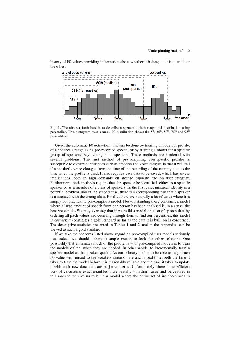
Furthermore, we want a model that is as general as possible. We will aim at finding a model capable of sensibly estimating speaker relative pitch by searching for (i) the trimmed pitch range of a speaker and (ii) a reasonable description of the distribution of pitch values within that range. Both (i) and (ii) can be approached by searching the F0 distribution for quantiles. Quantiles are values dividing an ordered set of observations. Phrased differently, a quantile is the cut-off point under which a certain proportion of the observations fall. Oft-used divisions have specific names, for example quartiles (which divide the observations into four equal parts), quintiles (five parts), deciles (10 parts), and percentiles (100 parts). For (i), the 5th and 95th percentile will be used as targets to achieve a trimming of the data. The exact numbers are ad hoc, although the techniques should not rely on the trimming being set at exactly five per cent at each end. For (ii), we will aim to further divide the speaker’s pitch values into four similarly sized parts – the quartiles. In other words, our aim is to find a method to decide if a pitch value is within a speakers range, given that we trim five per cent at the top and at the bottom of the range, and if so, which quartile of a speakers F0 distribution a given pitch value belongs to, with the first and fourth quartiles being somewhat diminished due to the trimming (see Fig. 1). Generally speaking, the task can be formulated as judging a given F0 value against some kind of

Underpinning /nailon/ 3

history of F0 values providing information about whether it belongs to this quantile or the other.

Fig. 1. The aim set forth here is to describe a speaker’s pitch range and distribution using percentiles. This histogram over a mock F0 distribution shows the 5th, 25th, 50th, 75th and 95th percentiles.

Given the automatic F0 extraction, this can be done by training a model, or profile, of a speaker’s range using pre-recorded speech, or by training a model for a specific group of speakers, say, young male speakers. These methods are burdened with several problems. The first method of pre-compiling user-specific profiles is susceptible to dynamic influences such as emotion and voice fatigue, in that it will fail if a speaker’s voice changes from the time of the recording of the training data to the time when the profile is used. It also requires user data to be saved, which has severe implications, both in high demands on storage capacity and on user integrity. Furthermore, both methods require that the speaker be identified, either as a specific speaker or as a member of a class of speakers. In the first case, mistaken identity is a potential problem, and in the second case, there is a corresponding risk that a speaker is associated with the wrong class. Finally, there are naturally a lot of cases where it is simply not practical to pre-compile a model. Notwithstanding these concerns, a model where a large amount of speech from one person has been analysed is, in a sense, the best we can do. We may even say that if we build a model on a set of speech data by ordering all pitch values and counting through them to find our percentiles, this model is correct; it constitutes a gold standard as far as the data it is built on is concerned. The descriptive statistics presented in Tables 1 and 2, and in the Appendix, can be viewed as such a gold standard.

If we take the concerns listed above regarding pre-compiled user models seriously – as indeed we should – there is ample reason to look for other solutions. One possibility that eliminates much of the problems with pre-compiled models is to train the models online, when they are needed. In other words, to incrementally train a speaker model as the speaker speaks. As our primary goal is to be able to judge each F0 value with regard to the speakers range online and in real-time, both the time it takes to train the model before it is reasonably reliable and the time it takes to update it with each new data item are major concerns. Unfortunately, there is no efficient way of calculating exact quantiles incrementally – finding range and percentiles in this manner requires us to build a model where the entire set of instances seen is


scanned to recalculate the range and percentiles each time a new instance is added. This method places high demands on memory and processor load. The relationship between the methods is the same as the relationship between the mean score and the median (indeed, if we aim to split a user’s pitch into two equally sized categories, say HIGH and LOW, then the mean or the median, respectively, would make up the threshold between the categories. All in all, the exact, instance based method of calculation is virtually useless for our purposes.

The stock pile way of getting around process intensive, instance based and exact calculation of distributions is to find some function that describes the data, either more or less exactly, as in the case of the colouring of rabbit youngs, or reasonably well, as when network and database engineers maintain estimated histograms [e.g. 13]. When it comes to the distribution of F0 values in a speaker’s speech, we and others have more or less treated them as if they were normally distributed [8, 14]. There are good reasons to suspect this not to be true. Several authors [e.g. 14] have also pointed out that the distribution is indeed not normal.

A quick survey of the F0 distributions of some individuals still leads one to believe that it is somewhere close to normal, and assuming a normal distribution allows us to straightforwardly find the percentiles given the standard deviation and the means, both of which are readily accessible in an incremental manner. The question, then, is: how close to the truth do we get if we assume a normally distributed F0 within a speaker’s speech?

Given our intention that the model be perceptually sound it is clear that we can disregard differences that cannot be perceived by humans. It is not entirely easy to say what differences in F0 humans can and cannot perceive, however. Several studies have been made on the subject: ‘t Hart, Collier, & Cohen [15] gives an overview of studies that place the just noticeable difference (JND) for F0 between 1 Hz and 5 Hz at frequencies around 100 Hz. Unsurprisingly, the higher values come from studies using voice like stimuli, and the lower from studies using sine tones and suchlike. Elsewhere, ‘t Hart reports the minimum difference between two F0 movements for them to be perceived as different. The numbers here are much larger, and range from over one and a half to more than four semitones [16]. For the purposes we have in mind – for example to classify pitch as HIGH, LOW, or MID within a speakers range - we will say that differences of less than one semitone are acceptable.

In the remainder of this chapter, we present the results of analyses of speech from eight speakers with a view to answering the following questions: What does the F0 distribution look like? How does a semitone transformation affect it? What will the error be if we assume normally distributed F0 values to approximate the 5th, 25th, 50th, 75th and 95th percentiles? How much speech is needed to build a reliable model of F0 distribution? Furthermore, we discuss whether there is a need for a decaying model – a model in which the weight of an observation decreases with time – and if so, what the rate of decay should be.


2 Method

2.1 Speech material

The speech data used for the present study consists of Swedish Map Task dialogues recorded by Pétur Helgason at Stockholm University [17, 18]. The Map Tasks were designed to elicit natural-sounding spontaneous dialogues [19]. There are two participants in a Map Task dialogue: an instruction-giver and an instruction follower. They each have a map, both maps being similar but not identical. For example, certain landmarks on these maps may be shared, whereas others are only present on one map, some landmarks occur on both maps but are in different positions etc. The task is for the instruction-giver to describe a route indicated on his or her map to the follower.

The Swedish Map Task data used in this study consists of recordings of four pairs, or eight speakers including five female (F1-F5) and three male (M1-M3) speakers. Within each pair, each speaker acted as both giver and follower at least once. They were recorded in an anechoic room, using close talking microphones, and facing away from each other. They were recorded on separate channels. The total duration of the complete speech material is about three hours.

2.2 F0 analysis and filtering

The Snack sound toolkit (http://www.speech.kth.se/snack/), with a pitch-tracker based on the ESPS tool get_f0 was used to extract F0 and intensity values. The resulting F0 values (in Hz) were transformed onto logarithmic scale (semitones relative to 100 Hz) to enable comparisons between Hertz and semitone data. Although the quality of the recordings was very good, there was some channel leakage. As the pitch-tracker analyzed parts of the leakage as voiced speech, a filter was used to remove the frames in the lower mode of the intensity distribution. Similarly, in case there was a bimodal distribution of F0 values (e.g. due to creaky voice or artefacts introduced by the pitch-tracker), another filter was applied to remove the lower mode of the F0 distribution. No filtering was used for the upper part of the distributions, however.

2.3 Statistical analysis

SPSS was used to calculate descriptive statistics, percentiles, and Kolmogorov-Smirnov tests of normality for Hertz and semitone data, respectively, in the pre-processed models condition.

For the incremental models condition the percentiles where calculated in two ways. A gold standard was achieved at each calculation interval by sorting and counting every data point, a method that, as already mentioned, is impractical for real, online purposes. Another set of function-based percentiles – which can be achieved realistically under real online circumstances – was then calculated in a two-step process, in which means and standard deviations were first calculated incrementally at


regular intervals. The straightforward method of doing this – simply adding up all instances and calculating the means and standard deviation using the sum and the number of instances – is associated with floating point errors which can be quite severe when the number of instances is high. Instead, recursion functions where used, as described by [20]. The percentiles where then looked up in a table of the area under the standard normal distribution [e.g. 21] using the incrementally calculated means and standard deviation. This technique is the same that we use in the /nailon/ software, although /nailon/ uses a very small moving window for get_f0 for performance reasons [10]. Here, in order to make the results of the incremental processing directly comparable to the pre-processed models created in SPSS, we used the same pre-extracted F0 values as input for all methods. An informal test revealed that /nailon/ data would yield very similar results, however.

3 Results: pre-processed models

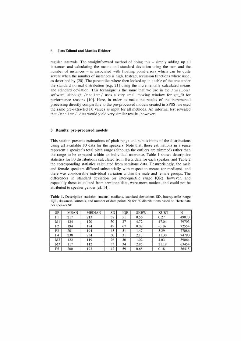
This section presents estimations of pitch range and subdivisions of the distributions using all available F0 data for the speakers. Note that, these estimations in a sense represent a speaker’s total pitch range (although the outliers are trimmed) rather than the range to be expected within an individual utterance. Table 1 shows descriptive statistics for F0 distributions calculated from Hertz data for each speaker, and Table 2 the corresponding statistics calculated from semitone data. Unsurprisingly, the male and female speakers differed substantially with respect to means (or medians), and there was considerable individual variation within the male and female groups. The differences in standard deviation (or inter-quartile range IQR), however, and especially those calculated from semitone data, were more modest, and could not be attributed to speaker gender [cf. 14].

Table 1. Descriptive statistics (means, medians, standard deviations SD, interquartile range IQR, skewness, kurtosis, and number of data points N) for F0 distributions based on Hertz data per speaker SP.

SP MEAN MEDIAN SD IQR SKEW. KURT. N F1 217 213 38 51 0.56 0.27 49070 M1 124 120 30 27 4.72 47.04 79703 F2 194 194 49 67 0.09 -0.16 72554 F3 201 194 45 51 1.47 5.29 77086 F4 238 234 30 31 2.13 11.30 74790 M2 122 119 26 30 1.02 4.03 39064 M3 117 112 33 34 2.85 21.19 63454 F5 200 193 42 59 0.68 0.18 36415


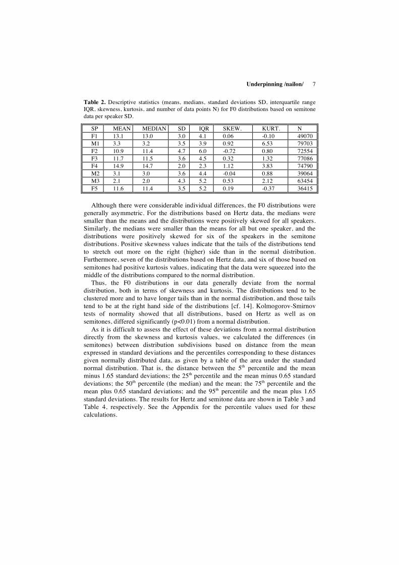
Table 2. Descriptive statistics (means, medians, standard deviations SD, interquartile range IQR, skewness, kurtosis, and number of data points N) for F0 distributions based on semitone data per speaker SD.

SP MEAN MEDIAN SD IQR SKEW. KURT. N F1 13.1 13.0 3.0 4.1 0.06 -0.10 49070 M1 3.3 3.2 3.5 3.9 0.92 6.53 79703 F2 10.9 11.4 4.7 6.0 -0.72 0.80 72554 F3 11.7 11.5 3.6 4.5 0.32 1.32 77086 F4 14.9 14.7 2.0 2.3 1.12 3.83 74790 M2 3.1 3.0 3.6 4.4 -0.04 0.88 39064 M3 2.1 2.0 4.3 5.2 0.53 2.12 63454 F5 11.6 11.4 3.5 5.2 0.19 -0.37 36415 Although there were considerable individual differences, the F0 distributions were

generally asymmetric. For the distributions based on Hertz data, the medians were smaller than the means and the distributions were positively skewed for all speakers. Similarly, the medians were smaller than the means for all but one speaker, and the distributions were positively skewed for six of the speakers in the semitone distributions. Positive skewness values indicate that the tails of the distributions tend to stretch out more on the right (higher) side than in the normal distribution. Furthermore, seven of the distributions based on Hertz data, and six of those based on semitones had positive kurtosis values, indicating that the data were squeezed into the middle of the distributions compared to the normal distribution.

Thus, the F0 distributions in our data generally deviate from the normal distribution, both in terms of skewness and kurtosis. The distributions tend to be clustered more and to have longer tails than in the normal distribution, and those tails tend to be at the right hand side of the distributions [cf. 14]. Kolmogorov-Smirnov tests of normality showed that all distributions, based on Hertz as well as on semitones, differed significantly (p<0.01) from a normal distribution.

As it is difficult to assess the effect of these deviations from a normal distribution directly from the skewness and kurtosis values, we calculated the differences (in semitones) between distribution subdivisions based on distance from the mean expressed in standard deviations and the percentiles corresponding to these distances given normally distributed data, as given by a table of the area under the standard normal distribution. That is, the distance between the 5th percentile and the mean minus 1.65 standard deviations; the 25th percentile and the mean minus 0.65 standard deviations; the 50th percentile (the median) and the mean; the 75th percentile and the mean plus 0.65 standard deviations; and the 95th percentile and the mean plus 1.65 standard deviations. The results for Hertz and semitone data are shown in Table 3 and Table 4, respectively. See the Appendix for the percentile values used for these calculations.


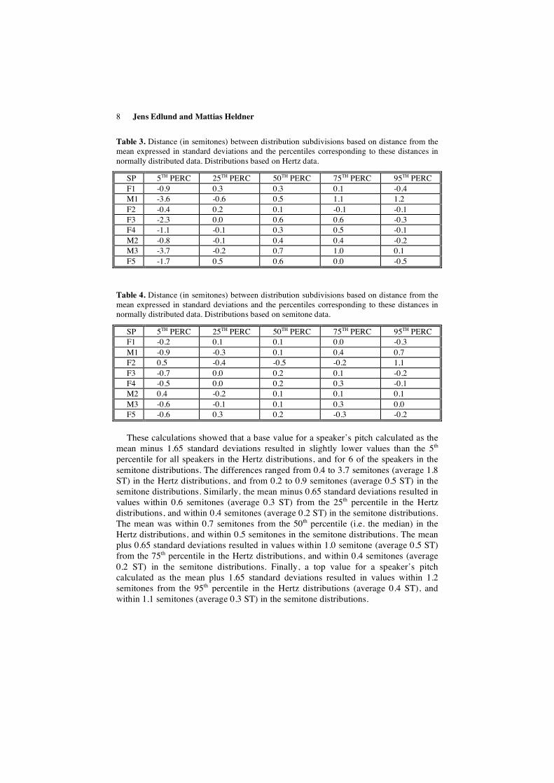
Table 3. Distance (in semitones) between distribution subdivisions based on distance from the mean expressed in standard deviations and the percentiles corresponding to these distances in normally distributed data. Distributions based on Hertz data.

SP 5TH PERC 25TH PERC 50TH PERC 75TH PERC 95TH PERC F1 -0.9 0.3 0.3 0.1 -0.4 M1 -3.6 -0.6 0.5 1.1 1.2 F2 -0.4 0.2 0.1 -0.1 -0.1 F3 -2.3 0.0 0.6 0.6 -0.3 F4 -1.1 -0.1 0.3 0.5 -0.1 M2 -0.8 -0.1 0.4 0.4 -0.2 M3 -3.7 -0.2 0.7 1.0 0.1 F5 -1.7 0.5 0.6 0.0 -0.5

Table 4. Distance (in semitones) between distribution subdivisions based on distance from the mean expressed in standard deviations and the percentiles corresponding to these distances in normally distributed data. Distributions based on semitone data.

SP 5TH PERC 25TH PERC 50TH PERC 75TH PERC 95TH PERC F1 -0.2 0.1 0.1 0.0 -0.3 M1 -0.9 -0.3 0.1 0.4 0.7 F2 0.5 -0.4 -0.5 -0.2 1.1 F3 -0.7 0.0 0.2 0.1 -0.2 F4 -0.5 0.0 0.2 0.3 -0.1 M2 0.4 -0.2 0.1 0.1 0.1 M3 -0.6 -0.1 0.1 0.3 0.0 F5 -0.6 0.3 0.2 -0.3 -0.2 These calculations showed that a base value for a speaker’s pitch calculated as the

mean minus 1.65 standard deviations resulted in slightly lower values than the 5th percentile for all speakers in the Hertz distributions, and for 6 of the speakers in the semitone distributions. The differences ranged from 0.4 to 3.7 semitones (average 1.8 ST) in the Hertz distributions, and from 0.2 to 0.9 semitones (average 0.5 ST) in the semitone distributions. Similarly, the mean minus 0.65 standard deviations resulted in values within 0.6 semitones (average 0.3 ST) from the 25th percentile in the Hertz distributions, and within 0.4 semitones (average 0.2 ST) in the semitone distributions. The mean was within 0.7 semitones from the 50th percentile (i.e. the median) in the Hertz distributions, and within 0.5 semitones in the semitone distributions. The mean plus 0.65 standard deviations resulted in values within 1.0 semitone (average 0.5 ST) from the 75th percentile in the Hertz distributions, and within 0.4 semitones (average 0.2 ST) in the semitone distributions. Finally, a top value for a speaker’s pitch calculated as the mean plus 1.65 standard deviations resulted in values within 1.2 semitones from the 95th percentile in the Hertz distributions (average 0.4 ST), and within 1.1 semitones (average 0.3 ST) in the semitone distributions.


4 Discussion: pre-processed models

The analyses of all F0 data for each speaker support the previous findings that F0 distributions are typically not normally distributed [cf. 12]. There is usually some positive skewness and some positive kurtosis indicating that the distributions lean to the right and are clustered more than the normal distribution. Thus, F0 data typically violate the assumption of normality underlying many statistical procedures, including estimations of pitch range based on means and standard deviations.

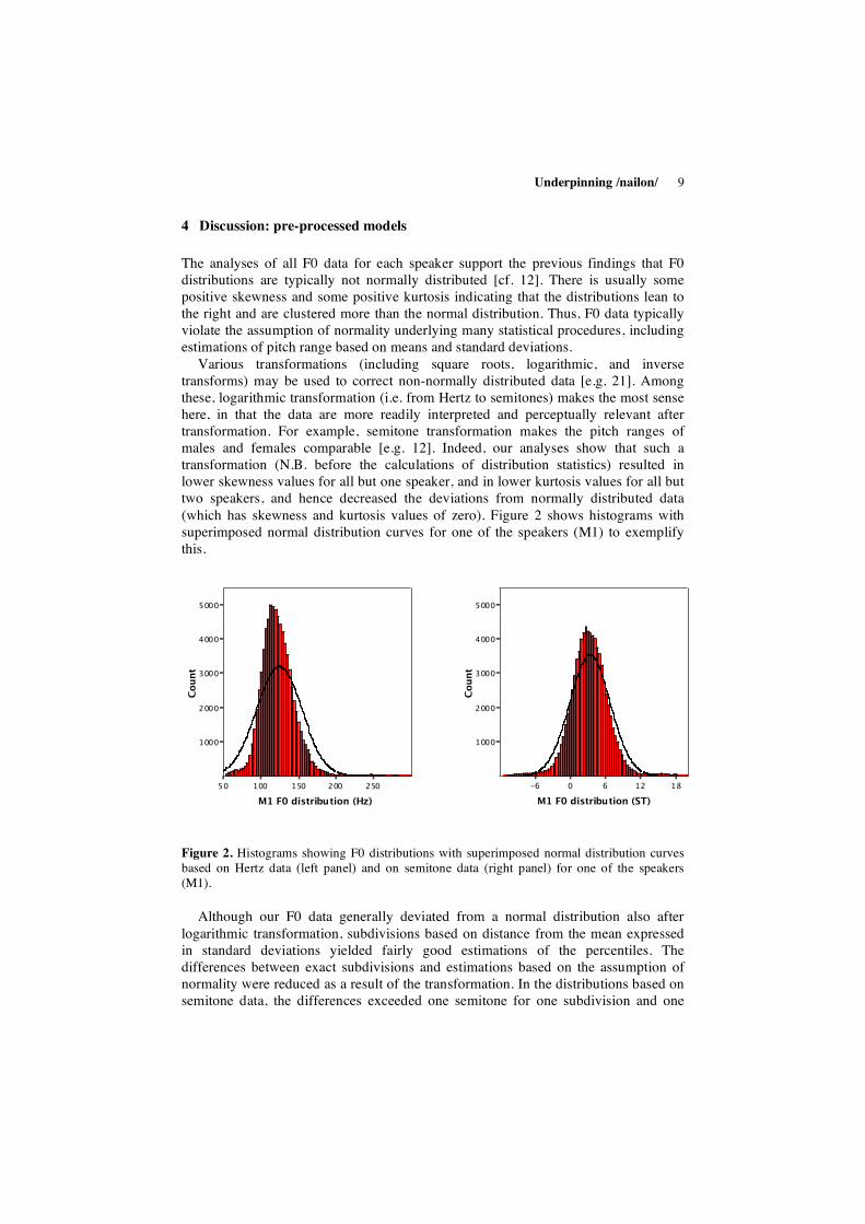
Various transformations (including square roots, logarithmic, and inverse transforms) may be used to correct non-normally distributed data [e.g. 21]. Among these, logarithmic transformation (i.e. from Hertz to semitones) makes the most sense here, in that the data are more readily interpreted and perceptually relevant after transformation. For example, semitone transformation makes the pitch ranges of males and females comparable [e.g. 12]. Indeed, our analyses show that such a transformation (N.B. before the calculations of distribution statistics) resulted in lower skewness values for all but one speaker, and in lower kurtosis values for all but two speakers, and hence decreased the deviations from normally distributed data (which has skewness and kurtosis values of zero). Figure 2 shows histograms with superimposed normal distribution curves for one of the speakers (M1) to exemplify this.

-6 0 6 12 18

M1 F0 distribution (ST)

1000

2000

3000

4000

5000

Count

Figure 2. Histograms showing F0 distributions with superimposed normal distribution curves based on Hertz data (left panel) and on semitone data (right panel) for one of the speakers (M1).

Although our F0 data generally deviated from a normal distribution also after logarithmic transformation, subdivisions based on distance from the mean expressed in standard deviations yielded fairly good estimations of the percentiles. The differences between exact subdivisions and estimations based on the assumption of normality were reduced as a result of the transformation. In the distributions based on semitone data, the differences exceeded one semitone for one subdivision and one

50 100 150 200 250

M1 F0 distribution (Hz)

1000

2000

3000

4000

5000

Count


speaker only (95th percentile, speaker F2). Given the current knowledge about pitch perception in speech [see e.g. 15 and references mentioned therein] we find it most unlikely that these differences should be perceptually relevant – we consider estimations within one semitone good enough for the kind of classification we are aiming at.

Based on these observations, we argue that use of semitone transformation is advantageous for theoretical as well as for statistical reasons, and hence a sound practice for automatic estimation of pitch range, and furthermore that distribution subdivisions based on means and standard deviations which in turn are based on a fair amount of data, yields a description of the F0 distribution that is good enough to estimate speaker relative pitch in an offline situation. It remains to be shown, however, how much speech is needed to build a reliable model of the F0 distribution in an online situation. This issue will be addressed in the following sections.

5 Results: incremental models

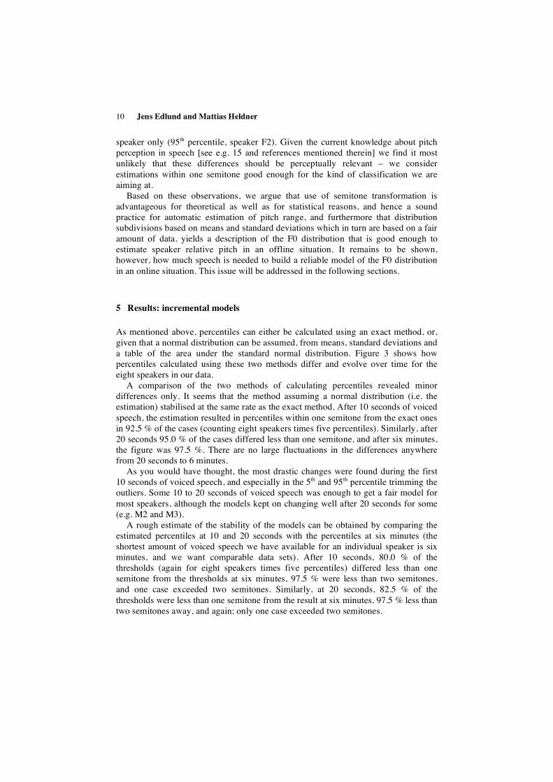
As mentioned above, percentiles can either be calculated using an exact method, or, given that a normal distribution can be assumed, from means, standard deviations and a table of the area under the standard normal distribution. Figure 3 shows how percentiles calculated using these two methods differ and evolve over time for the eight speakers in our data.

A comparison of the two methods of calculating percentiles revealed minor differences only. It seems that the method assuming a normal distribution (i.e. the estimation) stabilised at the same rate as the exact method. After 10 seconds of voiced speech, the estimation resulted in percentiles within one semitone from the exact ones in 92.5 % of the cases (counting eight speakers times five percentiles). Similarly, after 20 seconds 95.0 % of the cases differed less than one semitone, and after six minutes, the figure was 97.5 %. There are no large fluctuations in the differences anywhere from 20 seconds to 6 minutes.

As you would have thought, the most drastic changes were found during the first 10 seconds of voiced speech, and especially in the 5th and 95th percentile trimming the outliers. Some 10 to 20 seconds of voiced speech was enough to get a fair model for most speakers, although the models kept on changing well after 20 seconds for some (e.g. M2 and M3).

A rough estimate of the stability of the models can be obtained by comparing the estimated percentiles at 10 and 20 seconds with the percentiles at six minutes (the shortest amount of voiced speech we have available for an individual speaker is six minutes, and we want comparable data sets). After 10 seconds, 80.0 % of the thresholds (again for eight speakers times five percentiles) differed less than one semitone from the thresholds at six minutes, 97.5 % were less than two semitones, and one case exceeded two semitones. Similarly, at 20 seconds, 82.5 % of the thresholds were less than one semitone from the result at six minutes, 97.5 % less than two semitones away, and again; only one case exceeded two semitones.


Figure 3. Cumulative percentiles (in semitones) calculated using an exact method (black lines), and an estimation calculated from incremental means and standard deviations (grey lines) for each speaker. The 5th, 25th, 50th, 75th, and 95th percentiles are shown from the bottom and up. The scale on the time axis is logarithmic.

6 Discussion: incremental models

The analysis of the incremental models has shown that a good estimate of the shape of the F0 distribution can be obtained after a short period of time using incrementally calculated means and standard deviations, although it is clear that 10 to 20 seconds is not sufficient to create models of a speaker’s total pitch range. For most practical purposes, we would not be interested in a speaker’s total pitch range, however, but rather of a speaker’s current pitch range. We need to ask ourselves how stable F0-based models are, how much data needs to go into them, and when they become obsolete.

Figure 3 may lead us on our way towards the answers. It is important to note that if we use very large quantities of data in a model without putting less weight in old data than in new, we are quickly going to end up with a model that is in effect static, since each new data point has less and less influence on the model as a whole. Such a model will become increasingly burdened with problems typical for static models, most notably susceptibility to dynamic influences. If we on the other hand pay very little attention to older data, the model is going to flutter unpredictably. There are a number of ways to achieve a model that places more weight in new data than in old, for example by letting the weight of data points decrease as they grow older – a decaying model. The question is when the decay should start and at what speed it


should proceed. The graphs in Figure 3 indicate that in several cases, the models are quite fickle before the 10-second line. These fluctuations are not likely to be something we want to capture. At 20 seconds to a minute, the changes are much smaller and slower, and may well be worth modelling. A rough estimate, then, is that decay should commence no sooner than 10 seconds after the data is seen, and should continue slowly over 10 seconds to a minute, perhaps. Further research is needed to test these observations, however.

7 Conclusions

In this contribution, we have examined measurable manifestations of pitch range and speaker relative pitch in the speech signal and provided a hands-on description of how to capture this. The technique works and can be used on a normal computer under real-time online conditions. For concepts like “the centre of the user’s F0 range”, it is comparable to pre-processed models.

We may conclude that semitone transformation is advantageous for theoretical as well as for statistical reasons, and hence a sound practice for automatic estimation of pitch range, and furthermore that estimations of percentiles based on means and standard deviations yields a description of the F0 distribution that is good enough to estimate speaker relative pitch with errors of less than one semitone.

Finally, we note that somewhere between 10 and 20 seconds of voiced speech is sufficient training material to make such estimations for most speakers, at least in dialogue situations that change at a similar rate to Map Task, and that decaying models are likely to outperform models that grow rigid over large quantities of training data.

Acknowledgements. We thank Anders Eriksson and Rolf Carlson for their comments during this work. Any shortcomings in the present research remain our own. This work was carried out within the CHIL project. CHIL (Computers in the Human Interaction Loop) is an Integrated Project under the European Commission’s Sixth Framework Program (IP-506909).

References

1. Shriberg, E., Stolcke, A.: Direct Modeling of Prosody: An Overview of Applications in Automatic Speech Processing. In: Proceedings of Speech Prosody 2004 Nara, Japan. (2004) 575-582

2. Nilsonne, Å., Sundberg, J., Ternström, S., Askenfelt, A.: Measuring the Rate of Change of Voice Fundamental Frequency in Fluent Speech During Mental Depression. J. Acoust. Soc. Am. 83 (1987) 716-728

3. Bolinger, D.: Intonation and Its Uses: Melody in Grammar and Discourse. Edward Arnold, London (1989)


4. Carlson, R., Elenius, K., Swerts, M.: Perceptual Judgments of Pitch Range. In: Bel, B., Marlin, I. (eds.): Proceedings of the International Conference on Speech Prosody 2004, Nara, Japan. (2004) 689-692

5. Honorof, D.N., Whalen, D.H.: Perception of Pitch Location within a Speaker's F0 Range. J. Acoust. Soc. Am. 117 (2005) 2193-2200

6. Swerts, M., Veldhuis, R.: The Effect of Speech Melody on Voice Quality. Speech Com. 33 (2001) 297-303

7. Traunmüller, H.: Conventional, Biological and Environmental Factors in Speech Communication: A Modulation Theory. Phonetica. 51 (1994) 170-183

8. Edlund, J., Heldner, M.: Exploring Prosody in Interaction Control. Phonetica. 62 (2005) 215-226

9. Edlund, J., Heldner, M., Gustafson, J.: Utterance Segmentation and Turn-Taking in Spoken Dialogue Systems. In: Fisseni, B., Schmitz, H.-C., Schröder, B., Wagner, P. (eds.): Sprachtechnologie, mobile Kommunikation und linguistische Ressourcen. Peter Lang, Frankfurt am Main, Germany. (2005) 576-587

10. Edlund, J., Heldner, M.: /nailon/ – Software for Online Analysis of Prosody. In: Proceedings of the 9th International Conference on Spoken Language Processing (Interspeech 2006), Pittsburgh, PA, USA. (2006) 2022-2025

11. Hermes, D.J., van Gestel, J.C.: The Frequency Scale of Speech Intonation. J. Acoust. Soc. Am. 90 (1991) 97-102

12. Traunmüller, H., Eriksson, A.: The Perceptual Evaluation of F0 Excursions in Speech as Evidenced in Liveliness Estimations. J. Acoust. Soc. Am. 97 (1995) 1905-1915

13. Lam, E., Salem, K.: Dynamic Histograms for Non-Stationary Updates. In: Proceedings of the 9th International Database Engineering & Application Symposium (IDEAS'05). IEEE Computer Society. (2005) 235-243

14. Traunmüller, H., Eriksson, A.: The Frequency Range of the Voice Fundamental in the Speech of Male and Female Adults. [cited 2006-08-01]; Available from: http://www.ling.su.se/staff/hartmut/f0_m&f.pdf. (1995)

15. 't Hart, J., Collier, R., Cohen, A.: A Perceptual Study of Intonation: An Experimental-Phonetic Approach to Speech Melody. Cambridge Studies in Speech Science and Communication. Cambridge University Press, Cambridge (1990)

16. 't Hart, J.: Differential Sensitivity to Pitch Distance, Particularly in Speech. J. Acoust. Soc. Am. 69 (1981) 811-821

17. Helgason, P.: Preaspiration in the Nordic Languages: Synchronic and Diachronic Aspects. PhD dissertation. Department of Linguistics, Stockholm University, Stockholm (2002)

18. Helgason, P.: SMTC - A Swedish Map Task Corpus. In: Working Papers 52: Proceedings from Fonetik 2006. Lund University, Centre for Languages and Literature, Lund. (2006) 57-60

19. Anderson, A.H., Bader, M., Bard, E.G., Boyle, E., Doherty, G., Garrod, S., Isard, S., Kowtko, J., McAllister, J., Miller, J., Sotillo, C., Thompson, H., Weinert, R.: The HCRH Map Task Corpus. Lang. Speech. 34 (1991) 83-97

20. Welford, B.P.: Note on a Method for Calculating Corrected Sums of Squares and Products. Technometrics. 4 (1962) 419-420


21. Kirk, R.E.: Experimental Design: Procedures for the Behavioral Sciences. Third edn. Brooks/Cole Publishing Company, Pacific Grove, CA (1995)

Appendix

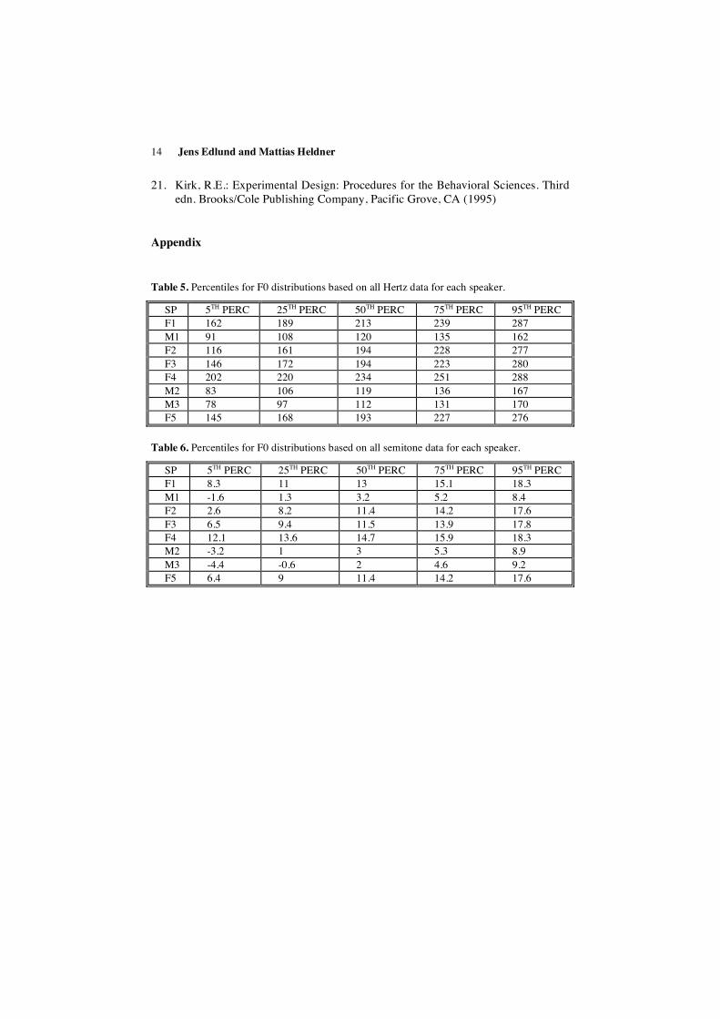
Table 5. Percentiles for F0 distributions based on all Hertz data for each speaker.

SP 5TH PERC 25TH PERC 50TH PERC 75TH PERC 95TH PERC F1 162 189 213 239 287 M1 91 108 120 135 162 F2 116 161 194 228 277 F3 146 172 194 223 280 F4 202 220 234 251 288 M2 83 106 119 136 167 M3 78 97 112 131 170 F5 145 168 193 227 276

Table 6. Percentiles for F0 distributions based on all semitone data for each speaker.

SP 5TH PERC 25TH PERC 50TH PERC 75TH PERC 95TH PERC F1 8.3 11 13 15.1 18.3 M1 -1.6 1.3 3.2 5.2 8.4 F2 2.6 8.2 11.4 14.2 17.6 F3 6.5 9.4 11.5 13.9 17.8 F4 12.1 13.6 14.7 15.9 18.3 M2 -3.2 1 3 5.3 8.9 M3 -4.4 -0.6 2 4.6 9.2 F5 6.4 9 11.4 14.2 17.6

Documents

Underpinning /nailon/: Automatic Estimation of Pitch Range