Takustraße 7D-14195 Berlin-Dahlem

GermanyKonrad-Zuse-Zentrumfur Informationstechnik Berlin

TIMO BERTHOLDAMBROS M. GLEIXNER

Undercovera primal MINLP heuristic exploring a largest sub-MIP

Supported by the DFG Research Center MATHEON Mathematics for key technologies in Berlin.

ZIB-Report 12-07 (February 2012)

Undercover

a primal MINLP heuristic exploring a largest sub-MIP

Timo Berthold∗ Ambros M. Gleixner†

February 2, 2012

Abstract

We present Undercover, a primal heuristic for nonconvex mixed-integer nonlinear pro-gramming (MINLP) that explores a mixed-integer linear subproblem (sub-MIP) of a givenMINLP. We solve a vertex covering problem to identify a minimal set of variables that needto be fixed in order to linearize each constraint, a so-called cover. Subsequently, these vari-ables are fixed to values obtained from a reference point, e.g., an optimal solution of a linearrelaxation. We apply domain propagation and conflict analysis to try to avoid infeasibilitiesand learn from them, respectively. Each feasible solution of the sub-MIP corresponds to afeasible solution of the original problem.

We present computational results on a test set of mixed-integer quadratically constrainedprograms (MIQCPs) and general MINLPs from MINLPLib. It turns out that the majorityof these instances allow for small covers. Although general in nature, the heuristic appearsmost promising for MIQCPs, and complements nicely with existing root node heuristics indifferent state-of-the-art solvers.

Keywords: Primal Heuristic, Mixed-Integer Nonlinear Programming, Large NeighborhoodSearch, Mixed-Integer Quadratically Constrained Programming, Nonconvex OptimizationMathematics Subject Classification: 90C11, 90C20, 90C26, 90C30, 90C59

1 Introduction

For mixed-integer (linear) programming it is well-known that, apart from complete solving meth-ods, general purpose primal heuristics like the feasibility pump [4, 19, 21] are able to find high-quality solutions for a wide range of problems. Over the years, primal heuristics have becomea substantial ingredient of state-of-the-art solvers for mixed-integer programming [6, 10]. Formixed-integer nonlinear programming (MINLP), the last three years saw an increasing interestof the research community in general-purpose primal heuristics [8, 9, 12, 13, 16, 30, 32, 33].

An MINLP is an optimization problem of the form

min dTx

s.t. gk(x) 6 0 for k = 1, . . . ,m,

Li 6 xi 6 Ui for i = 1, . . . , n,

xi ∈ Z for i ∈ I,

(1)

∗Zuse Institute Berlin, Takustr. 7, 14195 Berlin, Germany, berthold@zib.de†Zuse Institute Berlin, Takustr. 7, 14195 Berlin, Germany, gleixner@zib.de

1

where I ⊆ {1, . . . , n} is the index set of the integer variables, d ∈ Rn, gk : Rn → R for k =1, . . . ,m, and L ∈ (R∪{−∞})n, U ∈ (R∪{+∞})n are lower and upper bounds on the variables,respectively. Since fixed variables can always be eliminated, we assume w.l.o.g. that Li < Ui fori = 1, . . . , n, i.e., the interior of [L,U ] is nonempty. Note that a nonlinear objective function canalways be reformulated by introducing one additional constraint and variable, hence form (1) isgeneral.

If all constraint functions gk are quadratic we call (1) a mixed-integer quadratically constrainedprogram (MIQCP). If all constraints are linear we call (1) a mixed-integer program (MIP). If Iis empty, we refer to an MINLP, MIQCP, and MIP as a nonlinear program (NLP), quadraticallyconstrained program (QCP), and linear program (LP), respectively.

At the heart of many recently proposed primal MIP heuristics, such as Local Branching [20],RINS [17], DINS [23], and RENS [7], lies large neighborhood search, the paradigm of solving asmall sub-MIP that promises to contain good solutions. In this paper, we introduce Undercover, alarge neighborhood search start heuristic that constructs and solves a sub-MIP of a given MINLP.We demonstrate its effectiveness on a general test set of MIQCPs taken from the MINLPLib [14].

During the design of Undercover, our focus was its application as a start heuristic inside acomplete solver such as BARON [34], Couenne [5], Bonmin [11] or SCIP [3].

When primal heuristics are considered as standalone solving procedures, e.g., the RECIPEheuristic [30] or the Feasibility Pump [12, 16], the algorithmic design typically aims at findingfeasible solutions for as many instances as possible, even if this takes substantial running time.However, if they are used as supplementary procedures inside a complete solver, the overall solverperformance is the main objective. To this end, it is often worth sacrificing success on a smallnumber of instances for a significant saving in average running time. Primal heuristics in modernsolvers therefore often follow a “fast fail” strategy: the most crucial decisions are taken in thebeginning and in a defensive fashion such that if the procedure aborts, it will not have consumedmuch running time.

Two major features distinguish Undercover from all mentioned primal heuristics for MINLP.Firstly, unlike most of them [8, 12, 13, 16, 33], Undercover is not an extension of an existing MIPheuristic towards a broader class of problems; moreover, it does not have a counterpart in mixed-integer linear programming. Secondly, Undercover solves two auxiliary MIPs (one for finding aset of variables to be fixed plus the resulting sub-MIP), and at most two NLPs (possibly oneto compute initial fixing values, one for postprocessing the sub-MIP solution). To the contrary,most large neighborhood search heuristics [12, 16, 30, 32, 33] for MINLP solve an arbitrarily largeseries of MIPs, often alternated with a sequence of NLPs, to produce a feasible start solution.The number of iterations is typically not fixed, but depends on the instance at hand.

The paper is organized as follows. Section 2 introduces a first generic version of the Under-cover algorithm. In Section 3, we describe how to find variables to fix such that the resultingsubproblem is linear. Section 4 explains how to extract useful information, even if the sub-MIP proves to be infeasible. Finally, Section 6 provides computational results that show theeffectiveness of Undercover.

2 A generic algorithm

The paradigm of fixing a subset of the variables of a given mixed-integer program in order toobtain subproblems that are easier to solve has proven successful in many primal MIP heuristicssuch as RINS [17], DINS [23], and RENS [7]. The core difficulty in MIP solving is the integralityconstraints. Thus, in MIP context, “easy to solve” usually takes the meaning of few integervariables.

2

Actually, integrality is a special case of nonlinearity, since it is possible to model the integralityof a bounded integer variable xi ∈ {Li, . . . , Ui} by the nonconvex polynomial constraint (xi−Li)·. . .·(xi−Ui) = 0. This insight matches the practical experience that in MINLP, while integralitiesdo contribute to the complexity of the problem, the specific difficulty is the nonlinearities. Hence,“easy” in an MINLP context can be understood as few nonlinear constraints.

Our heuristic is based on the simple observation that by fixing certain variables (to somevalue within their bounds) any given mixed-integer nonlinear program can be reduced to amixed-integer linear subproblem (sub-MIP). Every feasible solution of this sub-MIP is then afeasible solution of the original MINLP.

Whereas in general it holds that many or even all of the variables might need to be fixedin order to arrive at a linear subproblem, our approach is motivated by the experience that forseveral practically relevant MINLPs fixing only a comparatively small subset of the variablesalready suffices to linearize the problem. The computational effort of solving this subproblemcompared to solving the original problem, however, is usually greatly reduced since we can applythe full strength of state-of-the-art MIP solving. Before formulating a first generic algorithm forour heuristic, consider the following definitions.

Definition 2.1. Let P be an MINLP of form (1) and C ⊆ {1, . . . , n} be a set of variable indicesof P . We call C a cover of constraint gk, k ∈ {1, . . . ,m}, if and only if the set

{(x, gk(x)) : x ∈ [L,U ], xi = x∗i for all i ∈ C} (2)

is affine for all x∗ ∈ [L,U ]. We call C a cover of P if and only if C is a cover of all con-straints g1, . . . , gm.

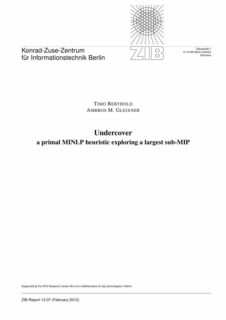
Figure 1: A convex MIQCP and the Undercover sub-MIP induced by the NLP relaxation.

The following example illustrates how covers of an MINLP are used to construct a sub-MIPfor finding feasible solutions.

Example 2.2 (the Undercover sub-MIP). Consider the following convex MIQCP:

min − y − zs.t. x+ y + z2 − 4 6 0

x, y, z > 0

x, y ∈ Z

(3)

3

The only variable that appears in a nonlinear term is z, hence {z} is the minimum coverof (3) w.r.t. the above definition. The (unique) optimal solution of its nonlinear relaxationis (0, 3.75, 0.5) with objective function value −4.25.

Taking that relaxation, the idea of Undercover is to fix z = 0.5, which makes (3) an integerlinear program. The (unique) optimal solution of this is (0, 3, 0.5) with objective function value−3.5, which is necessarily a feasible solution for the MIQCP (3). Taking the NLP as dual and theUndercover solution as primal bound, this gives an optimality gap of roughly 20%. The actual(unique) optimal solution of (3) is (0, 4, 0).

This example is illustrated in Figure 1. The light shaded region shows the solid correspondingto the NLP relaxation; the parallel lines show the mixed-integer set of feasible solutions of (3).The dark shaded area shows the polytope associated to the Undercover sub-MIP. The bluepoint B is the optimum of the NLP, the red point A is the optimum of the Undercover sub-MIP,the green point C is the optimum of the MIQCP. The smaller black points indicate furtherfeasible solutions of the Undercover sub-MIP.

A first generic algorithm for our heuristic is given in Figure 2. The clear hinge of the algorithmis found in line 5—finding a suitable cover of the given MINLP. Section 3 elaborates on this indetail.

input MINLP P as in (1)1

begin2

compute a solution x∗ of an approximation or relaxation of P3

round x∗i for i ∈ I4

determine a cover C of P5

solve the sub-MIP of P given by fixing xi = x∗i for all i ∈ C6

end7

Figure 2: Simple generic algorithm.

To obtain suitable fixing values for the selected variables, an approximation or relaxation ofthe original MINLP is used. For integer variables the approximate values are rounded. Mostcomplete solvers for MINLP are based on branch-and-bound [29]. If the heuristic is embeddedwithin a branch-and-bound solver, using its (linear or nonlinear) relaxation appears as a naturalchoice for obtaining approximate variable values.

Large neighborhood search heuristics that rely on fixing variables typically have to trade offbetween eliminating many variables in order to make the sub-MIP tractable and leaving enoughdegrees of freedom such that the sub-MIP is still feasible and contains good solutions. Oftentheir implementation inside a MIP solver demands a sufficiently large percentage of variables tobe fixed to arrive at an easy to solve sub-MIP [6, 7, 17, 23].

For our heuristic, the situation is different since we do not aim to eliminate integrality con-straints, but nonlinearities. While it still holds that fixing variables, even only few, results in asmaller search space, the main benefit is that we arrive at a MIP.

In a nutshell: instead of solving an easier problem of the same class, we solve a smallerproblem of an easier class.

In order to linearize a given MINLP, in general we may be forced to fix integer and continuousvariables. The fixing of continuous variables, especially, in an MINLP can introduce a significanterror, even rendering the subproblem infeasible. Thus our heuristic will aim at fixing as fewvariables as possible to obtain as large a linear subproblem as possible, through the utilizationof minimum covers.

4

3 Finding minimum covers

This section describes our method for determining a minimum cover of an MINLP, i.e., a minimalsubset of variables to fix in order to linearize each constraint. In this section, we make thestandard assumption that the nonlinear functions involved are twice continuously differentiable.However, the idea of Undercover can easily be applied to MINLPs in general, as will be explainedin Section 7. Note that the partial derivatives are well-defined since the domain [L,U ] hasnonempty interior.

As motivation let us first consider bilinear programs, i.e., QCPs with a bipartition of theirvariables, {1, . . . , n} = A ∪ B, A ∩ B = ∅, and each quadratic term of the form xixj , i ∈ A,j ∈ B. In this case, holding the variables of either A or B fixed, per definition one obtains alinear program—a simple property that has been used extensively in various solution approaches.The sets A and B each constitutes a cover. In the global optimization literature, the variablescorresponding to the smaller of both sets are often called complicating variables. If the partitioninto A and B is unique, then these complicating variables form a minimum cover.

Any general quadratically constrained program can be converted to a bilinear program byduplication of variables. Hansen and Jaumard [26] showed how to perform this transformationsuch as to minimize either the number of duplicated or complicating variables. The followingdefinition is a straightforward generalization of their notion of a co-occurrence graph to MINLPs.

Definition 3.1 (co-occurrence graph). Let P be an MINLP of form (1) with g1, . . . , gm twicecontinuously differentiable on [L,U ]. We call GP = (V,E) the co-occurrence graph of P withnode set VP = {1, . . . , n} given by the variable indices of P and edge set

EP ={ij | i, j ∈ V,∃k ∈ {1, . . . ,m} :

∂2

∂xi∂xjgk(x) 6≡ 0

},

i.e., we draw an edge between i and j if and only if the Hessian matrix of some constraint has astructurally nonzero entry (i, j).

Remark 3.2. Since the Hessian of a twice continuously differentiable function is symmetric,GP is a well-defined, undirected graph. It may contain loops, e.g., if square terms x2i are present.Trivially, the co-occurrence graph of a bilinear program is bipartite; the co-occurrence graph of aMIP is an edge-free graph.

Theorem 3.3. Let P be an MINLP of form (1) with g1, . . . , gm twice continuously differentiableon [L,U ]. Then C ⊆ {1, . . . , n} is a cover of P if and only if it is a vertex cover of the co-occurrence graph GP .

Proof. If h : Rn → R is twice continuously differentiable, x∗i ∈ Rn, C ⊆ {1, . . . , n}, then fixingvariables xi = x∗i , i ∈ C, and projecting to the nonfixed variables yields another twice continu-ously differentiable function h : Rn−|C| → R. Let π : Rn → Rn−|C| be the projection x 7→ (xi)i 6∈C .

Now the Hessian matrix of h is simply obtained from the Hessian of h by taking the columnsand rows of nonfixed variables:

∇2hπ(x) =( ∂2

∂xi∂xjh(x)

)i,j 6∈C

for any x ∈ Rn with xi = x∗i , i ∈ C. A twice continuously differentiable function is affine if andonly if its Hessian vanishes on its domain. Hence,

C is a cover of h⇔ ∀i, j 6∈ C :∂2

∂xi∂xjh(x) ≡ 0.

5

For the MINLP P this yields that

C is a cover of P ⇔ ∀i, j 6∈ C, k ∈ {1, . . . ,m} :∂2

∂xi∂xjgk(x) ≡ 0

⇔ ∀i, j 6∈ C : ij 6∈ EP⇔ ∀ij ∈ EP d : i ∈ C ∨ j ∈ C,

i.e., if and only if C is a vertex cover of the co-occurrence graph GP .

Note that any undirected graph G = (V,E) is the co-occurrence graph of the QCP min{0 :xixj 6 0 for all ij ∈ E}. Hence, minimum vertex cover can be transformed to computing aminimum cover of an MINLP. Since minimum vertex cover is NP-hard [22], we have

Corollary 3.4. Computing a minimum cover of an MINLP is NP-hard.

There exist, however, many polynomial-time algorithms to approximate a minimum vertexcover within a factor of 2, such as simply taking the vertices of a maximal matching. It isconjectured that 2 is also the optimal approximation factor [28] and it is proven that vertexcover is NP-hard to approximate within a factor smaller than 10

√5−21 = 1.3606 . . . [18], hence

no polynomial-time approximation scheme exists. Approximation ratios 2−ε(G) are known withε(G) > 0 depending on special properties of the graph such as number of nodes [27] or boundeddegree [25].

In this paper we aim at computing minimum covers exactly. For this we use a simple binaryprogramming formulation. For an MINLP of form (1), define auxiliary binary variables αi,i = 1, . . . , n, equal to 1 if and only if the original variable xi is fixed. Then

C(α) := {i ∈ {1, . . . , n} : αi = 1}

forms a cover of P if and only if αi + αj > 1 for all ij ∈ EP . For an MIQCP, e.g., this requiresall square terms and at least one variable in each bilinear term to be fixed. To obtain as large alinear subproblem as possible, we solve the binary program

min{ n∑i=1

αi : αi + αj > 1 for all ij ∈ EP , α ∈ {0, 1}n}

(4)

minimizing the sum of auxiliary variables.Note that for particular classes of MINLPs it is possible to exploit special features of the

co-occurrence graph in order to compute a minimum cover exactly in polynomial time—a simpleexample is the class of bilinear programs mentioned above—or to approximate it within a factorsufficiently close to 1. However, in our experiments the binary program (4) could always besolved by a standard MIP solver within a fraction of a second. In all cases, optimality wasproven at the root node, hence without enumeration.

4 Domain propagation and conflict learning

Fixing a variable can have great impact on the original problem and the approximation we use.An important detail, crucial for the success rate of Undercover, is not to fix the variables in thecover simultaneously, but sequentially one by one. This section describes how we use domainpropagation, backtracking and conflict analysis to avoid and handle infeasibilities during thisprocess.

6

Fix-and-propagate. The task of domain propagation is to analyze the individual structureof single constraints w.r.t. the current domains of the variables in order to infer additionaldomain reductions, thereby tightening the search space. For an overview of domain propagationtechniques applied in MIP and MINLP solvers, see [3] and [35], respectively.

To prevent obvious infeasibilities, we fix the variables in the cover one after the other applyingdomain propagation after each fixing in order to further tighten the bounds, in particular of theyet unfixed cover variables. During this process, it might happen that the value a variable takesin the reference solution is no longer contained in its reduced domain. In this case, we insteadfix the variable to the closest bound.1 This fix-and-propagate procedure resembles a methoddescribed in [21]. Additionally, we apply it for continuous variables.

Note that by this, the fixing values and hence the created subproblem depend on the fixing or-der. Different variable orderings lead to different propagations, thereby to different subproblemsand different solutions being found.

Of course, it might also happen that a variable domain becomes empty. This means thatthe subproblem with the currently chosen fixing values is proven to be infeasible without evenhaving started its solution procedure.

In this case, we apply a one-level backtracking, i.e., we undo the last bound change and tryalternative fixing values, see Section 5 for details. Note that if we cannot resolve the infeasibilityby one-level backtracking, Undercover will terminate. This is a “fast fail” strategy: if we cannoteasily resolve the infeasibility, we abort at an early stage of the algorithm without wasting runningtime.2

Even if fix-and-propagate runs into an infeasibility, we can extract useful information for theglobal solution process. Adding so-called conflict constraints prevents running into the samedeadlock twice.

Conflict analysis in MIP. Conflict learning is a technique that analyzes infeasible subprob-lems encountered during a branch-and-bound search. Whenever a subproblem is infeasible,conflict analysis can be used to learn one (or more) reasons for this infeasibility. This gives riseto so called conflict constraints that can be exploited in the remainder of the search to pruneother parts of the tree.

Carefully engineered conflict analysis has lead to a substantial increase in the size of problemsmodern SAT solvers can deal with [31]. It has recently been generalized to MIP [1, 2]. One maindifference between MIP and SAT solving in the context of conflict analysis is that the variablesof a MIP do not need to be of binary type. In [1] it is shown how the concept of a conflict graphcan be extended to MIPs with general integer and continuous variables.

The most successful SAT learning approaches use so called first unique implication point(1UIP) learning, which captures a conflict that is “close” to the infeasibility and can infer newinformation. Solvers for MIP or MINLP typically take a longer processing time per node andthey do not restart during search. That is why MIP solvers with conflict learning such as SCIPpotentially generate several conflicts for each infeasibility.

Conflict analysis for Undercover. The fix-and-propagate strategy can be seen as a simula-tion of a depth-first-search in the branch-and-bound tree, applying one-level backtracking when afixing results in an infeasible subproblem. Hence, using conflict analysis for these partially fixed,infeasible subproblems enables us to learn constraints that are valid for the global search of the

1Alternatively, we could recompute the reference solution to obtain values within the current bounds.2If we want to apply Undercover more aggressively, we can try to recover from infeasibility by reordering

the fixing sequence, e.g., such that the variable for which the fixing failed will be the first one in the reorderedsequence. This resembles a simple restarting mechanism from SAT solving.

7

original MINLP. This is done by building up the conflict graph that is implied by the variablefixings and the propagated bound changes. For this, the reason for each propagation, i.e., thebounds of other variables that implied the domain reduction, needs to be stored or reconstructedlater on.

Note that the generated conflict constraints will not be limited to the variables in the coversince the conflict graph also contains all variables that have changed their bounds due to domainpropagation in the fix-and-propagate procedure.

Valid constraints can be learned even after fix-and-propagate. If the subsequent sub-MIPsolution process proves infeasibility and all variables in the cover are integer, we may forbid theassignment made to the cover variables for the global solution process. The same constraintcan be learned if the Undercover sub-MIP could be solved to proven optimality, since the searchspace that is implied by these fixings has been fully explored. In both cases, this is particularlyuseful for small covers.

5 The complete algorithm

This section outlines the details of the complete Undercover algorithm, cf., Figure 3. In the firststep, we construct the covering problem (4) by collecting the edges of the co-occurrence graph,see Section 3. For constraints of simple form such as quadratic ones the sparsity pattern of theHessian matrix can be read directly from the description of the constraint function. For generalnonlinearities, we use algorithmic differentiation to automatically compute the sparsity patternof the Hessian, see, e.g., [24].

To solve the covering problem we employ a standard MIP solver, which in our computationalexperiments never took more than a fraction of a second to find an optimal cover. Nevertheless,since the covering problem is NP-hard, solving it to optimality may be time-consuming, ingeneral. To safeguard against this, we only solve the root node and proceed with the best solutionfound. Subsequently, we fix the variables in the computed cover as described in Section 4.3

As motivated in the beginning, we designed Undercover to be applied within a complete solver.During fix-and-propagate, we call two routines provided by the solver, domain propagation inline 23 and conflict analysis in line 27. If the former detects infeasibility, we call the latter tolearn conflict constraints for the global solution process, see Section 4.

If domain propagation detects infeasibility after fixing variable xi, i ∈ C, to the (rounded andprojected) value Xi in the reference solution, we try to recover by one-level backtracking. Thefollowing alternatives will be tried: for binary variables the value 1−Xi; for nonbinary variablesthe lower bound Li and, if this is also infeasible, the upper bound Ui. In the case of infinitebounds Li and Ui are replaced by Xi − |Xi| and Xi + |Xi|, respectively. If Xi = 0, then −1 and+1 will be used instead. Of course, if fixing values accidentally coincide, each value is testedonly once.

Typically, the sub-MIP solved in the next step incurs the highest computational effort and iscontrolled by work limits on the number of nodes, LP iterations, etc., see Section 6 for details.Since by construction the sub-MIP should be significantly easier than the original MINLP, we

3If we want to apply Undercover aggressively and allow for solving the covering problem multiple times, thefollowing two strategies can be used. First, during the fix-and-propagate routine variables outside the precomputedcover may be fixed simultaneously. In this case, the fixing of some of the yet unfixed variables in the cover mightbecome redundant. Recomputing the cover with αi = 1 for all i with local bounds Li = Ui may yield a smallernumber of remaining variable fixings. Second, if no feasible fixings for the cover variables are found later on, wecan re-solve the covering problem adding a cutoff constraint

∑i∈C(1−αi)+

∑i6∈C αi > 1 and try again. However,

both techniques appear to be computationally too expensive for the standard setting that we explored in ourcomputational experiments.

8

input MINLP as in (1), reference point x∗ ∈ [L,U ], ni > 0 alternative fixingvalues y∗i,1, . . . , y

∗i,ni∈ [Li, Ui] for all i ∈ {1, . . . , n}

output feasible solution x (on success)

begin/* Step 1: create covering problem */

E ← ∅ /* edge set of co-occurrence graph */1

foreach k ∈ {1, . . . ,m} do2

Sk ← {i ∈ {1, . . . , n} : gk depends on xi} /* variables in gk(x) 6 0 */3

foreach i ∈ Sk do4

if∂2

∂x2igk(x) 6≡ 0 then E ← E ∪ {(i, i)} /* must fix xi */

5

else6

foreach j ∈ Sk, j > i,∂2

∂xi∂xjgk(x) 6≡ 0 do

7

E ← E ∪ {(i, j)} /* must fix xi or xj */8

/* Step 2: solve covering problem (4) */

α∗ ← arg min{∑n

i=1 αi : αi + αj > 1 for all ij ∈ E,α ∈ {0, 1}n}

9

C ← {i ∈ {1, . . . , n} : α∗i = 1}10

/* Step 3: fix-and-propagate loop */

L← L, U ← U /* local bounds */11

foreach i ∈ C do12

L0 ← L, U0 ← U , p← 0 /* store bounds for backtracking */13

X ← ∅, success← false /* set of failed fixing values */14

while ¬success and p 6 ni do15

Xi ← if p = 0 then x∗i else y∗i,p16

if i ∈ I then Xi ← [Xi] /* round if variable integer */17

X ← min{max{Xi, Li}, Ui} /* project to bounds if outside */18

if Xi ∈ X then19

p← p+ 1 /* skip fixing values tried before */20

else21

Li ← Xi, Ui ← Xi /* fix */22

call domain propagation on [L, U ] /* propagate */23

if [L, U ] 6= ∅ then24

success← true /* accept fixing, go to next variable */25

else26

call conflict analysis27

L← L0, U ← U0 /* infeasible: backtrack */28

X ← X ∪ {Xi}, p← p+ 1 /* try next fixing value */29

if ¬success then return /* no feasible fixing found: terminate */30

/* Step 4: solve sub-MIP */

solve sub-MIP min{dTx : gk(x) 6 0 for k = 1, . . . ,m,

Li 6 xi 6 Ui for i = 1, . . . , n, xi ∈ Z for i ∈ I}

31

if sub-MIP solved to optimality or proven infeasible and C ⊆ I then32

add constraint∨

i∈C(xi 6= Xi) to original problem33

/* Step 5: solve sub-NLP */

if feasible sub-MIP solution found then34

x← best sub-MIP solution35

if sub-MIP not solved to optimality or C 6⊆ I then36

/* restore global bounds, fix integers, solve locally */

solve sub-NLP min{dTx : gk(x) 6 0 for k = 1, . . . ,m,

Li 6 xi 6 Ui for i = 1, . . . , n, xi = xi for i ∈ I}

37

x← sub-NLP solution /* update sub-MIP solution */38

return x39

end

Figure 3: The complete Undercover algorithm.

9

expect that often it can indeed be solved to optimality or proven infeasible. As described inSection 4, we may then forbid the assignment of fixing values to the cover variables if the latterare all integer, stated in line 33.

Eventually, if a feasible sub-MIP solution x has been found, we try to improve it further byfixing all integer variables to their values in x and solving the resulting NLP to local optimality.Clearly, if all cover variables are integer and x is optimal for the sub-MIP, this step can beskipped. Otherwise, we reoptimize over the continuous variables in the cover and may obtain abetter objective value.

6 Computational experiments

Only few solvers exist that handle nonconvex MINLPs, such as BARON [34], Couenne [5],and LindoGlobal [40]. Others, e.g., Bonmin [11] and SBB [41], guarantee global optimality onlyfor convex problems, but can be used as heuristic solvers for nonconvex problems. Recently,the solver SCIP [2, 3] was extended to solve nonconvex MIQCPs [9] and MINLPs [35] to globaloptimality. For a comprehensive survey of available MINLP solver software, see [15].

Experimental setup. The target of our computational experiments was to analyze the per-formance of Undercover as a start heuristic for MINLPs applied at the root node. Therefore,we evaluated the sizes of the actual covers found, the success rate of Undercover, the distribu-tion of running time among different components of the algorithm, and benchmarked againststate-of-the-art solvers.

We implemented the algorithm given in Figure 3 within SCIP4 and used SCIP’s LP solutionas reference point x∗. To perform the fix-and-propagate procedure, we called the standarddomain propagation engine of SCIP. Secondary SCIP instances were used to solve both thecovering problem (4) and the Undercover sub-MIP.

We controlled the computational effort for solving the sub-MIP in two ways. First, we imposeda hard limit of 500 nodes and a dynamic stall node limit5 between 1 and 500 nodes. Second,we adjusted the SCIP settings to find feasible solutions fast: we disabled expensive presolvingtechniques and used the “primal heuristics emphasis aggressive” and the “emphasis feasibility”settings. Furthermore, if the sub-MIP is infeasible, this is often detected already when solvingthe root relaxation, hence we deactivated expensive pre-root heuristics so as to not lose time onsuch instances. Components using sub-MIPs themselves are switched off altogether. For details,please refer to the source code at [38].

In our main experiment, we ran SCIP with all heuristics other than Undercover switchedoff and cut generation deactivated. We used SCIP 2.1.1 with CPLEX 12.3 [39] as LP solver,Ipopt 3.10 [36] as NLP solver for the postprocessing, and CppAD 20100101.4 [37] as expressioninterpreter for evaluating general nonlinear constraints. We refer to this configuration as UC.

We tested against the state-of-the-art MINLP solvers BARON 9.3.1 [34] (commercial license),Couenne 0.3 [5] (open source), and SCIP 2.1.1 (academic license) with Undercover disabled. Inorder to investigate how Undercover can enhance the root node performance of complete solvers,we compare UC with their root heuristics. SCIP, for instance, applies eleven primal heuristicsat the root node.

As test set we used a selection of 37 MIQCP instances from MINLPLib [14]. We excludedlop97ic, lop97icx, pb302035, pb351535, qap, and qapw, which are linear after the default pre-

4The source code is publicly available within SCIP 2.1.1 and can be found at [38].5With a stall node limit we terminate if no improving solutions are found within a certain number of branch-

and-bound nodes since the discovery of the current incumbent.

10

Cover Fix&Prop MIP NLP Misc

Figure 4: Distribution of running time among different components of Undercover heuristic.

solving of SCIP. On the nuclear instances, the root LP relaxation of SCIP is often unboundeddue to unbounded variables in nonconvex terms of the constraints. In this case, we cannot ap-ply Undercover since no fixing values are available. Due to this, we only included two of thoseinstances, nuclear14a and nuclear14b, for which the root LP of SCIP is bounded.

We further tested Undercover on general MINLPs from MINLPLib, excluding those whichare MIQCPs, linear after SCIP presolving, or contain expressions that cannot be handled bySCIP, e.g., sin and cos. Additionally, three more instances with unbounded root LP relaxationwere removed, leaving 110 instances. We used the same settings and solvers as described above.

All experiments were conducted on a 3.00 GHz Intel Core 2 Extreme CPU X9650 with6144 KB Cache and 8 GB RAM using openSuse 11.4 with compiler GCC 4.5.1. Hyperthreadingand Turboboost were disabled.

Results for MIQCP. The results for the experiments on MIQCPs are shown in Table 1.In columns “% cov” and “% nlcov”, we report the relative size of the cover used by UC aspercentage of the total number of variables and of the number of variables that appear in at leastone nonlinear term, respectively. All numbers are calculated w.r.t. the numbers of variables afterpreprocessing. Note that a value of 100% in the “% nlcov” column means that the trivial coverconsisting of all variables appearing in nonlinear terms is already minimal. For all other instances,the solution of the covering problem gives rise to a smaller cover, hence a larger sub-MIP andpotentially more solutions for the MINLP.

Column “UC” shows the objective value of the best solution found by Undercover. Forall other solvers, we provide the objective value of the best solution found during root nodeprocessing. The best objective value among the four columns is marked bold.

The computational results for MIQCPs seem to confirm our expectation that often a lowfixing rate suffices to obtain a linear subproblem: 13 of the instances in our test set allow a coverof at most 5% of the variables, further 13 instances of at most 25%. Only 5 instances were ina medium range of 25%–50%, for another 6 a minimum cover contained more than 80% of thevariables.

UC found a feasible solution for 24 test instances: on 11 out of the 13 instances with a coverof at most 5% of the variables, on 8 out of 13 instances with a cover of at most 25%, and on 5out of the remaining 11 instances. In comparison, BARON found a feasible solution in 18 cases,Couenne in 6, SCIP in 25. UC found an optimal solution for instances ex1266, sep1, st_e31,and tloss, and a solution within less than 0.1% gap to the optimal solution value for instancesfac3, and util.

There were 10 instances for which UC found a solution, but BARON did not, 4 times itwas the other way around. Comparing UC to Couenne, this ratio is 20 : 2, w.r.t. SCIP it is8 : 9. We note that on 7 instances UC found a solution, although none of BARON, Couenne,and SCIP did. For 11 instances UC found the single best solution and for 3 further instances itproduced the same solution quality as the best of the other solvers.

The time for applying Undercover was always less than 0.3 seconds, except for the instance

11

waste, for which Undercover ran for 2.5 seconds. Figure 4 shows the average distribution ofrunning time spent for solving the covering problem, processing the fix-and-propagate loop,solving the sub-MIP, polishing the solution with an NLP solver and for the remaining parts suchas allocating and freeing data structures, constructing the auxiliary problems, computing conflictconstraints, and so on. This average has been taken over all instances for which Undercoverfound a feasible solution, hence all main parts of the algorithm have been executed. The majoramount of time, namely 60%, is spent in solving the sub-MIP. Solving the covering problem plusperforming fix-and-propagate took only about 15% of the actual running time.

Although the polytope described by (4) is not integral, the covering problem could always besolved to optimality in the root node by SCIP’s default heuristics and cutting plane algorithms.In 23 out of 37 cases, the minimal cover was nontrivial, with cover sizes of 8–50% of the nonlinearvariables.

We note that in 11 out of the 13 cases for which the resulting sub-MIP was infeasible, theinfeasibility was already detected during the fix-and-propagate stage, in the remaining two casesduring root node processing of the sub-MIP. Thus in most cases, no time was wasted to try tofind a solution for an infeasible subproblem, since the most expensive part, see Figure 4, can beskipped. This confirms that Undercover follows a “fast fail” strategy, a beneficial property ofheuristic procedures applied within complete solvers, as argued in Section 1. Also, all feasible sub-MIPs could be solved to optimality within the imposed node limit of 500, which indicates that—with a state-of-the-art MIP solver at hand—the generated subproblems are indeed significantlyeasier than the full MIQCP.

For 14 out of 24 successful runs, all cover variables were integral. For the remaining 10instances, NLP postprocessing was applied; 7 times, it could further improve the Undercoversolution.

Recall that an arbitrary point x∗ ∈ [L,U ] can serve as reference solution for Undercover. Anatural alternative to the LP solution is a (locally) optimal solution of the NLP relaxation. Anadditional experiment showed that, using an NLP solution, Undercover only succeeded in findinga feasible solution for 18 instances of the MIQCP test set, instead of 24. If both versions founda solution, the quality of the one based on the NLP solution was better in eight cases, worse inthree. Our interpretation for the lower success rate is that the advantage of the NLP solution,namely being feasible for all nonlinear constraints, is dominated by the fact that an NLP solutiontypically has a higher fractionality, which leads to a higher chance that infeasibility is introducedin line 17 of the Undercover algorithm in Figure 3.

Results for MINLP. As expected, Undercover is much less powerful for general MINLPscompared to MIQCPs. UC produced feasible solutions for only six out of more than a hundredtest problems from MINLPLib. During root node processing, BARON found feasible solutionsfor 39 instances, Couenne for 23, SCIP for 35. Table 2 shows results only for those instanceson which Undercover succeeded. Although it is clearly outperformed by the other solvers w.r.t.the number of solutions found, we would like to mention that for each other solver there is atleast one instance for which UC succeeded, but the solver did not.

Nevertheless, the experiments showed that fixing a small fraction of the variables would oftenhave sufficed to obtain a linear subproblem: for 77 out of the 110 test instances, the minimumcover contained at most 25% of the variables, similar to the MIQCP case, but only 5 MINLPsallowed for a cover size below 5%. Hence, compared to the MIQCP test set, cover sizes areon average larger and very small covers occur rarely, but this alone does not explain the lowersuccess rate. It simply appears to be more difficult to find feasible fixing values due to the highercomplexity of the nonlinear constraints, even if we use the solution of an NLP relaxation asthe reference point x∗. Curiously enough, Undercover produced feasible solutions for the two

12

instances with smallest and the two instances with largest minimum cover.

Further experiments. We experimented with the following extensions of Undercover: re-ordering the fixing sequence if fix-and-propagate fails, see Footnote 2; re-solving the coveringproblem if the sub-MIP is infeasible, see Footnote 3; using a weighted version of the coveringproblem, see Section 7. None of those performed significantly better than our default strategy.

In a complete solver, primal heuristics are applied in concert, hence a feasible solution may bealready at hand when starting Undercover. In our implementation, this is exploited in two ways.First, we use values from the incumbent solution as fixing alternatives during fix-and-propagate.Fixing the variables to values in the incumbent has the advantage that the resulting sub-MIP isguaranteed to be feasible, compare, e.g., [17]. Second, we add a primal cutoff to the sub-MIP toonly look for improving solutions.6 On four instances of the MIQCP testset, SCIP 2.1.1 withdefault heuristics including Undercover produced a primal solution that was significantly betterthan the best solution found by either SCIP or Undercover alone; a worse solution was producedonly for one instance.

7 Variants

We experimented with a few more variants of the Undercover heuristic. Some of them provedbeneficial for specific problem classes. For the standard setting presented in our computationalresults, however, they showed no significant impact. As they might prove useful for futureapplications of Undercover, we will give a brief description.

Our initial motivation for using a minimum cardinality cover was to minimize the impacton the original MINLP. Instead of measuring the impact of fixing variables uniformly, we couldsolve a weighted version of the covering problem (4). To better reflect the problem structure,the objective coefficients of the auxiliary variables αi could be computed from characteristics ofthe original variables xi such as the domain size, variable type, or appearance in nonlinear termsor constraints violated by the reference solution.

Instead of fixing the variables in a cover, we could also merely reduce their domains to asmall neighborhood around the reference solution. Especially for continuous variables this leavesmore freedom to the subproblem explored and can lead to better solutions found. Of course,the difficulty of solving the subproblem is increased. Nevertheless, small domains may allow forsufficiently tight underestimators for an MINLP solver to tackle the subproblem.

The main idea of Undercover is to reduce the computational effort by switching to a problemclass that is easier to address. While we have focused on exploring a linear subproblem, fornonconvex MINLPs, convex subproblems may provide a larger neighborhood to be searched andstill be sufficiently easy to solve.

8 Conclusion

In this paper, we have introduced Undercover, a primal MINLP heuristic exploring large linearsubproblems induced by a minimum vertex cover. It differs from other recently proposed MINLPheuristics in that it is neither an extension of an existing MIP heuristic, nor solves an entiresequence of MIPs.

We defined the notion of a minimum cover of an MINLP and proved that it can be computedby solving a vertex covering problem on the co-occurrence graph induced by the sparsity patterns

6A primal cutoff is an upper bound on the objective function that results in branch-and-bound nodes withworse dual bound not being explored.

13

of the Hessians of the nonlinear constraint functions. Although NP-hard, in our experimentscovering problems could be solved rapidly. Several extensions and algorithmic details have beendiscussed.

Undercover exploits the fact that small covers correspond to large sub-MIPs. We showedthat most instances of the MINLPLib [14] allow for covers consisting of at most 25% of theirvariables.

In particular for MIQCPs, Undercover proved to be a fast start heuristic, that often producesfeasible solutions of reasonable quality. The computational results indicate, that it complementsnicely with existing root node heuristics in different solvers. Undercover is now one of the defaultheuristics applied in SCIP.

Acknowledgements

Many thanks to Tobias Achterberg, Christina Burt, and Stefan Vigerske for their valuable com-ments. This research has been supported by the DFG Research Center Matheon Mathematicsfor key technologies in Berlin, http://www.matheon.de.

References

[1] Achterberg, T.: Conflict analysis in mixed integer programming. Discrete Optimization4(1), 4–20 (2007)

[2] Achterberg, T.: Constraint integer programming. Ph.D. thesis, Technische UniversitatBerlin (2007)

[3] Achterberg, T.: SCIP: Solving Constraint Integer Programs. Mathematical ProgrammingComputation 1(1), 1–41 (2009)

[4] Achterberg, T., Berthold, T.: Improving the feasibility pump. Discrete Optimization 4(1),77–86 (2007)

[5] Belotti, P., Lee, J., Liberti, L., Margot, F., Wachter, A.: Branching and bounds tighteningtechniques for non-convex MINLP. Optimization Methods & Software 24, 597–634 (2009)

[6] Berthold, T.: Primal heuristics for mixed integer programs. Diploma thesis, TechnischeUniversitat Berlin (2006)

[7] Berthold, T.: RENS – Relaxation Enforced Neighborhood Search. ZIB-Report 07-28, ZuseInstitute Berlin (2007)

[8] Berthold, T., Heinz, S., Pfetsch, M.E., Vigerske, S.: Large neighborhood search beyondMIP. In: L.D. Gaspero, A. Schaerf, T. Stutzle (eds.) Proceedings of the 9th MetaheuristicsInternational Conference (MIC 2011), pp. 51–60 (2011)

[9] Berthold, T., Heinz, S., Vigerske, S.: Extending a CIP framework to solve MIQCPs. In:J. Lee, S. Leyffer (eds.) Mixed Integer Nonlinear Programming, The IMA Volumes in Math-ematics and its Applications, vol. 154, pp. 427–444. Springer (2011)

[10] Bixby, R., Fenelon, M., Gu, Z., Rothberg, E., Wunderling, R.: MIP: Theory and practice– closing the gap. In: M. Powell, S. Scholtes (eds.) Systems Modelling and Optimization:Methods, Theory, and Applications, pp. 19–49. Kluwer Academic Publisher (2000)

14

[11] Bonami, P., Biegler, L., Conn, A., Cornuejols, G., Grossmann, I., Laird, C., Lee, J., Lodi,A., Margot, F., Sawaya, N., Wachter, A.: An algorithmic framework for convex mixedinteger nonlinear programs. Discrete Optimization 5, 186–204 (2008)

[12] Bonami, P., Cornuejols, G., Lodi, A., Margot, F.: A feasibility pump for mixed integernonlinear programs. Mathematical Programming 119(2), 331–352 (2009)

[13] Bonami, P., Goncalves, J.: Heuristics for convex mixed integer nonlinear programs. Com-putational Optimization and Applications pp. 1–19 (2010)

[14] Bussieck, M., Drud, A., Meeraus, A.: MINLPLib – a collection of test models for mixed-integer nonlinear programming. INFORMS Journal on Computing 15(1), 114–119 (2003)

[15] Bussieck, M.R., Vigerske, S.: MINLP solver software. In: J.J. Cochran, L.A. Cox, P. Ke-skinocak, J.P. Kharoufeh, J.C. Smith (eds.) Wiley Encyclopedia of Operations Research andManagement Science. Wiley and Sons, Inc. (2010)

[16] D’Ambrosio, C., Frangioni, A., Liberti, L., Lodi, A.: Experiments with a feasibility pumpapproach for nonconvex MINLPs. In: P. Festa (ed.) Experimental Algorithms, Lecture Notesin Computer Science, vol. 6049, pp. 350–360. Springer Berlin / Heidelberg (2010)

[17] Danna, E., Rothberg, E., Pape, C.L.: Exploring relaxation induced neighborhoods to im-prove MIP solutions. Mathematical Programming 102(1), 71–90 (2004)

[18] Dinur, I., Safra, S.: On the hardness of approximating vertex cover. Annals of Mathematics162, 439–485 (2005)

[19] Fischetti, M., Glover, F., Lodi, A.: The feasibility pump. Mathematical Programming104(1), 91–104 (2005)

[20] Fischetti, M., Lodi, A.: Local branching. Mathematical Programming 98(1-3), 23–47 (2003)

[21] Fischetti, M., Salvagnin, D.: Feasibility pump 2.0. Mathematical Programming Computa-tion 1, 201–222 (2009)

[22] Garey, M.R., Johnson, D.S.: Computers and Intractability: A Guide to the Theory ofNP-Completeness. W. H. Freeman & Co., New York, NY, USA (1979)

[23] Ghosh, S.: DINS, a MIP improvement heuristic. In: Proceedings of the 12th IPCO, pp.310–323 (2007)

[24] Griewank, A., Walther, A.: Evaluating derivatives: principles and techniques of algorithmicdifferentiation. Society for Industrial and Applied Mathematics (SIAM) (2008)

[25] Halperin, E.: Improved approximation algorithms for the vertex cover problem in graphsand hypergraphs. SIAM Journal on Computation 31, 1608–1623 (2002)

[26] Hansen, P., Jaumard, B.: Reduction of indefinite quadratic programs to bilinear programs.Journal of Global Optimization 2(1), 41–60 (1992)

[27] Karakostas, G.: A better approximation ratio for the vertex cover problem. ACM Transac-tions on Algorithms 5, 41:1–41:8 (2009)

[28] Khot, S., Regev, O.: Vertex cover might be hard to approximate to within 2− ε. Journal ofComputer and System Sciences 74(3), 335–349 (2008). Computational Complexity 2003

15

[29] Land, A.H., Doig, A.G.: An automatic method of solving discrete programming problems.Econometrica 28(3), 497–520 (1960)

[30] Liberti, L., Mladenovic, N., Nannicini, G.: A recipe for finding good solutions to MINLPs.Mathematical Programming Computation 3, 349–390 (2011)

[31] Moskewicz, M., Madigan, C., Zhao, Y., Zhang, L., Malik, S.: Chaff: Engineering an efficientSAT solver. In: Proceedings of DAC’01, pp. 530–535 (2001)

[32] Nannicini, G., Belotti, P.: Rounding-based heuristics for nonconvex MINLPs. MathematicalProgramming Computation (2011)

[33] Nannicini, G., Belotti, P., Liberti, L.: A local branching heuristic for MINLPs. ArXive-prints (2008)

[34] Tawarmalani, M., Sahinidis, N.: Global optimization of mixed-integer nonlinear programs:A theoretical and computational study. Mathematical Programming 99, 563–591 (2004)

[35] Vigerske, S.: Decomposition in multistage stochastic programming and a constraint integerprogramming approach to mixed-integer nonlinear programming. Ph.D. thesis, Humboldt-Universitat zu Berlin (2012). Submitted

[36] Wachter, A., Biegler, L.: On the implementation of a primal-dual interior point filterline search algorithm for large-scale nonlinear programming. Mathematical Programming106(1), 25–57 (2006)

[37] CppAD. A Package for Differentiation of C++ Algorithms. http://www.coin-or.org/

CppAD/

[38] SCIP. Solving Constraint Integer Programs. http://scip.zib.de/

[39] IBM ILOG CPLEX Optimizer. http://www.cplex.com/

[40] LindoGlobal. Lindo Systems, Inc. http://www.lindo.com

[41] SBB. ARKI Consulting & Development A/S and GAMS Inc. http://www.gams.com/

solvers/solvers.htm#SBB

16

Table 1: Computational results on MIQCP instances.

instance % cov % nlcov UC BARON Couenne SCIP

du-opt5 94.74 100.00 546.280975 – 157.082231 15.62177du-opt 95.24 100.00 632.891424 108.331477 3.905155 4.904642elf 5.56 50.00 1.675 1.675 – 0.328ex1263 4.40 20.00 30.1 – – –ex1264 4.88 20.00 11.1 – – –ex1265 4.10 16.67 15.1 – – –ex1266 3.57 14.29 16.3 – – –fac3 80.60 100.00 31995143.5 72826487.6 – 32039523.2feedtray2 4.67 50.00 – – – 0meanvarx 23.33 100.00 14.824808 14.369232 14.404062 14.369212netmod dol1 0.30 100.00 0 -0.250023 – -0.372303netmod dol2 0.38 100.00 0 0.0571641 – 0netmod kar1 0.88 100.00 0 -0.364809 – 0netmod kar2 0.88 100.00 0 -0.364809 – 0nous1 29.79 36.84 – – 1.567072 –nous2 30.43 36.84 – 0.625967 0.625967 1.384316nuclear14a 12.24 48.98 – -1.129079 – -1.100766nuclear14b 12.24 48.98 – – – -1.097686nvs19 88.89 100.00 – -1098 – -1097.8nvs23 90.00 100.00 484.2 -1124.8 – -1122.2nvs24 90.91 100.00 – -1027.4 – -1028.8product2 23.80 100.00 – – – -2102.377product 36.22 100.00 – – – -2094.688sep1 10.53 40.00 -510.081 -510.081 -510.081 -470.13space25a 5.84 41.86 – – – –space25 1.04 30.77 – – – –space960 27.74 43.43 – – – 17130000spectra2 44.12 100.00 306.3343 119.8743 – 13.97830st e31 3.39 40.00 -2 -2 – –tln12 6.67 8.33 – – – –tln5 14.29 16.67 15.1 – – 15.5tln6 12.50 14.29 32.3 – – –tln7 11.11 12.50 30.3 – – –tloss 13.04 14.29 16.3 – – –tltr 16.07 33.33 61.133333 – – 83.475util 3.12 16.67 999.690564 999.57875 – 1005.26814waste 2.50 13.78 661.337258 684.087647 – 692.983766

17

Table 2: Computational results on selected MINLP instances.

instance % cov % nlcov UC BARON Couenne SCIP

mbtd 0.18 0.18 9.00006 – 9.6667 –nvs09 85.00 87.18 28.865663 – -43.134337 -9.451041nvs20 96.97 100.00 3276194408 230.922165 258.96067 –stockcycle 9.98 100.00 357714.332 433304.376 – 306163.247synthes1 33.33 100.00 6.009759 6.009759 7.092732 6.009759johnall 0.14 0.16 -224.73017 -222.373032 -224.73017 -224.73017

18