1

An Efficient Multiperiod MINLP Model for Optimal

Planning of Offshore Oil and Gas Field Infrastructure

Vijay Gupta* and Ignacio E. Grossmann

†

Department of Chemical Engineering, Carnegie Mellon University

Pittsburgh, PA 15213

Abstract

In this paper, we present an efficient strategic/tactical planning model for offshore oilfield

development problem that is fairly generic and can be extended to include other complexities.

The proposed multiperiod non-convex MINLP model for multi-field site includes three

components (oil, water and gas) explicitly in the formulation using 3rd

and higher order

polynomials avoiding bilinear and other nonlinear terms. With the objective of maximizing total

NPV for long-term planning horizon, the model involves decisions related to FPSO (floating

production, storage and offloading) installation and expansion schedule and respective oil, liquid

and gas capacities, connection between the fields and FPSOs, well drilling schedule and

production rates of these three components in each time period. The resulting model can be

solved effectively with DICOPT for realistic instances and gives good quality solutions.

Furthermore, the model can be reformulated into an MILP after piecewise linearization and exact

linearization techniques that can be solved globally in an efficient way. Solutions of realistic

instances involving 10 fields, 3 FPSOs, 84 wells and 20 years planning horizon are reported, as

well as comparisons between the computational performance of the proposed MINLP and MILP

formulations.

Keywords: multiperiod optimization, planning, Offshore Oil and Gas field development, MINLP,

Investment and operations planning, FPSO

*E-mail: vijaygup@andrew.cmu.edu

†To whom all correspondence should be addressed. E-mail: grossmann@cmu.edu

2

1 Introduction

Offshore oil and gas field development represents a very complex problem and involves multi-

billion dollar investments and profits (Babusiaux et al., 2004). The complexity comes from the

fact that usually there are many alternatives available for installation of the platforms and their

sizes, for deciding which fields to develop and what should be the order to develop them, and

which and how many wells are to be drilled in those fields and in what order, which field to be

connected to which facility, and how much oil and gas to produce from each field. The

sequencing of these installations and connections must also be based on physical considerations,

e.g. field can only be developed if a corresponding facility is present. The other complexities are

the consideration of nonlinear profiles of the reservoir that are critical to predict the actual

flowrates of oil, water and gas from each field as there can be significant variations in these

flowrates over time, limitation on the number of wells that can be drilled each year due to

availability of the drilling rigs, and long-term planning horizon that is the characteristics of the

these projects. Moreover, installation and operation decisions in these projects involve very large

investments that can lead to large profits, or losses in the worst case if these decisions are not

made carefully.

Therefore, based on the above, there is a clear motivation to optimize the investment and

operations decisions for oil and gas field development problem to ensure reasonable return on the

investments over the time horizon considered. By including all the considerations described

above in an optimization model, this leads to a multiperiod MINLP problem. Furthermore, the

extension of this model to the cases where we consider the fiscal rules (Van den Heever et al.

(2000) and Van den Heever and Grossmann (2001)) and the uncertainties, especially endogenous

uncertainty cases (Jonsbraten et al. (1998), Goel and Grossmann (2004, 2006), Goel et al. (2006),

Tarhan et al. (2009, 2011) and Gupta and Grossmann (2011)), can lead to a very complex

problem to solve. Therefore, an effective model for the deterministic case is proposed that on the

one hand captures the realistic reservoir profiles, interaction among various fields and facilities,

wells drilling limitations and other practical trade-offs involved in the offshore development

planning, and on the other hand can be used as the basis for extensions that include other

complexities, especially fiscal rules and uncertainties. This paper focuses on a non-convex

MINLP model for the strategic/tactical planning of the offshore oil and gas fields, which

3

includes sufficient details to make it useful for realistic oilfield development projects, as well as

for extensions to include fiscal and uncertainty considerations.

The oilfield investment and operation planning is traditionally modeled as separate LP

(Lee and Aranofsky (1958), Aronofsky and Williams (1962)) or MILP (Frair, 1973) problems

under certain assumptions to make them computationally tractable. Simultaneous optimization of

the investment and operation decisions was addressed in Bohannon (1970), Sullivan (1982) and

Haugland et al. (1988) using MILP formulations with different levels of details in these models.

Behrenbruch (1993) emphasized the need to consider a correct geological model and to

incorporate flexibility into the decision process for an oilfield development project.

Iyer et al. (1998) proposed a multiperiod MILP model for optimal planning and

scheduling of offshore oilfield infrastructure investment and operations. The model considers the

facility allocation, production planning, and scheduling within a single model and incorporates

the reservoir performance, surface pressure constraints, and oil rig resource constraints. To solve

the resulting large-scale problem, the nonlinear reservoir performance equations are

approximated through piecewise linear approximations. As the model considers the performance

of each individual well in a reservoir independently, it becomes expensive to solve for realistic

multi-field sites. Moreover, the flow rate of water was not considered explicitly for facility

capacity calculations.

Van den Heever and Grossmann (2000) extended the work of Iyer et al. (1998) and

proposed a multiperiod generalized disjunctive programming model for oil field infrastructure

planning for which they developed a bilevel decomposition method. As opposed to Iyer and

Grossmann (1998), they explicitly incorporated a nonlinear reservoir model into the formulation.

Van den Heever et al. (2000), and Van den Heever and Grossmann (2001) extended their work to

handle complex economic objectives including royalties, tariffs, and taxes for the multiple gas

fields site. These authors incorporated these complexities into their model through disjunctions

as well as big-M formulations. The results were presented for realistic instances involving 16

fields and 15 years. However, the model considers only gas production and the number of wells

were used as parameters (fixed well schedule) in the model.

Ortiz-Gomez et al. (2002) presented three mixed integer multiperiod optimization models

of varying complexity for the oil production planning. The problem considers fixed topology and

is concerned with the decisions involving the oil production profiles and operation/shut in times

4

of the wells in each time period assuming nonlinear reservoir behavior. Based on the continuous

time formulation for gas field development with complex economics, Lin and Floudas (2003)

presented an MINLP model and solved it with a two stage algorithm. Carvalho and Pinto (2006)

considered an MILP formulation for oilfield planning based on the model developed by

Tsarbopoulou (2000), and proposed a bilevel decomposition algorithm for solving large scale

problems where master problem determines the assignment of platforms to wells and a planning

subproblem calculates the timing for the fixed assignments. The work was further extended by

Carvalho and Pinto (2006) to consider multiple reservoirs within the model.

In the papers described above, one of the major assumptions is that there is no uncertainty

in the parameters. Jonsbraten (1998) addressed the oilfield development planning problem under

oil price uncertainty using an MILP formulation which was solved with a progressive hedging

algorithm. Aseeri et al. (2004) introduced uncertainty in the oil prices and well productivity

indexes, financial risk management, and budgeting constraints into the model proposed by Iyer

and Grossmann (1998) and solved the resulting stochastic model using a sampling average

approximation algorithm. Goel and Grossmann (2004) considered a gas field development

problem under uncertainty in the size and quality of reserves where decisions on the timing of

field drilling were assumed to yield an immediate resolution of the uncertainty, i.e. the problem

involves decision-dependent uncertainty as discussed in Jonsbraten et al. (1998). Linear reservoir

models, which can provide a reasonable approximation for gas fields, were used. In their solution

strategy, the authors used a relaxation problem to predict upper bounds, and solved multistage

stochastic programs for a fixed scenario tree for finding lower bounds. Goel et al. (2006) later

proposed a branch and bound algorithm for solving the corresponding disjunctive/mixed-integer

programming model where lower bounds are generated by Lagrangean duality.

Ulstein et al. (2007) addressed the tactical planning of petroleum production that involves

regulation of production levels from wells, splitting of production flows into oil and gas

products, further processing of gas and transportation in a pipeline network. The model was

solved for different cases with demand variations, quality constraints, and system breakdowns.

Tarhan et al. (2009) developed a multistage stochastic programming model for planning offshore

oil field infrastructure under uncertainty where the uncertainties in initial maximum oil flowrate,

recoverable oil volume, and water breakthrough time of the reservoir are revealed gradually as a

function of investment and operating decisions. The model is formulated as a disjunctive/mixed-

5

integer nonlinear programming model that consists of individual non-convex MINLP

subproblems connected to each other through initial and conditional non-anticipativity

constraints. The duality-based branch and bound algorithm was proposed taking advantage of the

problem structure and globally optimizing each scenario problem independently. However, it

considers either gas/water or oil/water components for single field and single reservoir at a

detailed level. Hence, realistic multi-field site instances can be expensive to solve with this

model.

Li et al. (2010) presented a stochastic pooling optimization formulation to address the

design and operation of natural gas production networks, where the qualities of the flows are

described with a pooling model and the uncertainty is handled with a two-stage stochastic

approach. The resulting large-scale nonconvex MINLP is solved with a rigorous decomposition

method. Elgsæter et al. (2010) proposed a structured approach to optimize offshore oil and gas

production with uncertain models which iteratively updates setpoints while documenting the

benefits of each proposed setpoint change through excitation planning and result analysis. The

approach is able to realize a significant portion of the available profit potential while ensuring

feasibility despite large initial model uncertainty.

In this paper, there are six major extensions and differences that are addressed as

compared to the previous work:

(1) We consider all three components (oil, water and gas) explicitly in the formulation,

which allows to consider realistic problems for facility installation and capacity decisions.

(2) Nonlinear reservoir behavior in the model is approximated by 3rd and higher order

polynomials to ensure sufficient accuracy for the predicted reservoir profiles.

(3) Reservoir profiles are modeled as independent polynomials for each field-facility

connections for simplicity.

(4) The number of wells is used as a variable for each field to capture the realistic drill rig

limitations and the resulting trade-offs among various fields.

(5) We include the possibility of expanding the facility capacities in the future, and

including the lead times for construction and expansions for each facility to ensure realistic

investments.

(6) Reservoir profiles are also expressed in terms of cumulative water and cumulative gas

produced that are derived from WOR and GOR expressions avoiding bilinearities in the model.

6

The outline of this paper is as follows. First, we present a brief background on the basic

structure of an offshore oilfield site and major reservoir features. Next, we introduce the problem

statement and the MINLP model for offshore oilfield development problem. The MINLP model

is then reformulated as an MILP problem. Furthermore, both models are reformulated with

reduced number of binary variables. Numerical results of three realistic cases up to 10 oilfields

and 20 years are considered to report the performance of the proposed models.

2 Background

An offshore oilfield infrastructure consists of various production facilities such as Floating

Production, Storage and Offloading (FPSO), fields, wells and connecting pipelines to produce oil

and gas from the reserves. Each oilfield consists of a number of potential wells to be drilled

using drilling rigs, which are then connected to the facilities through pipelines to produce oil.

There is two-phase flow in these pipelines due to the presence of gas and liquid that comprises

oil and water. Therefore, there are three components, and their relative amounts depend on

certain parameters like cumulative oil produced. The field to facility connection involves trade-

offs associated to the flowrates of oil and gas for a particular field-facility connection,

connection costs, and possibility of other fields to connect to that same facility, while the number

of wells that can be drilled in a field depends on the availability of the drilling rig that can drill a

certain number of wells each year.

We assume in this paper that the type of offshore facilities connected to fields to produce

oil and gas are FPSOs with continuous capacities and ability to expand them in the future. These

FPSO facilities costs multi-billion dollars each depending on their sizes and have the capability

of operating in remote locations for very deep offshore oilfields (200m-2000m) where seabed

pipelines are not cost effective. FPSOs are large ships that can process the produced oil and store

until it is shipped to the onshore site or sales terminal. Processing includes the separation of oil,

water and gas into individual streams using separators located at these facilities. Each FPSO

facility has a lead time between the construction or expansion decision, and the actual

availability. The wells are subsea wells in each field that are drilled using drilling ships.

Therefore, there is no need to have a facility present to drill a subsea well. The only requirement

to recover oil from it is that the well must be connected to a FPSO facility. In this paper, we

focus on multi-field site and include sufficient details in the model to account for the various

trade-offs involved without going into much detail for each of these fields. However, the

7

proposed model can easily be extended to include various facility types and other details in the

oilfield development planning problem.

The location of production facilities and possible field and facility allocation itself is a

very complex problem. In this work, we assume that the potential location of facilities and field-

facility connections are given. In addition, the potential number of wells in each field is also

given. Note that each field can be potentially allocated to more than one FPSO facility, but once

the particular field-connection is selected, the other possibilities are not considered. Furthermore,

each facility can be used to produce oil from more than one field.

The facilities and connection involved in the offshore planning are often in operation

over many years, and it is therefore important to take future conditions into consideration when

designing an initial infrastructure or any expansions. This can be incorporated by dividing the

planning horizon, for example, 20 years, into a number of time periods with a length of 1 year,

and allowing investment and operating decisions in each period, which leads to a multi-period

planning problem.

fig 1

0

2

4

6

8

10

12

14

0 0.2 0.4 0.6 0.8 1

x (k

stb

/d)

fc

Oil Deliveribility per well

x(F1-FPSO1)

x(F1-FPSO2)

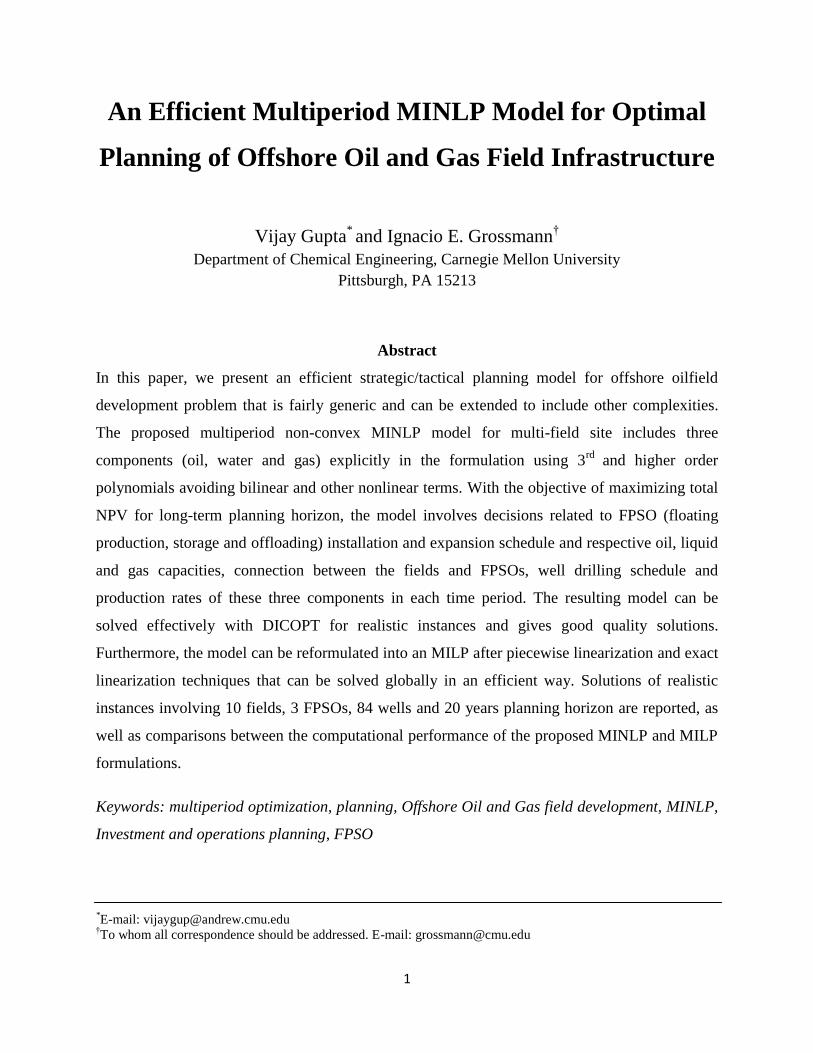
(a) Oil Deliverability per well for field (F1)

8

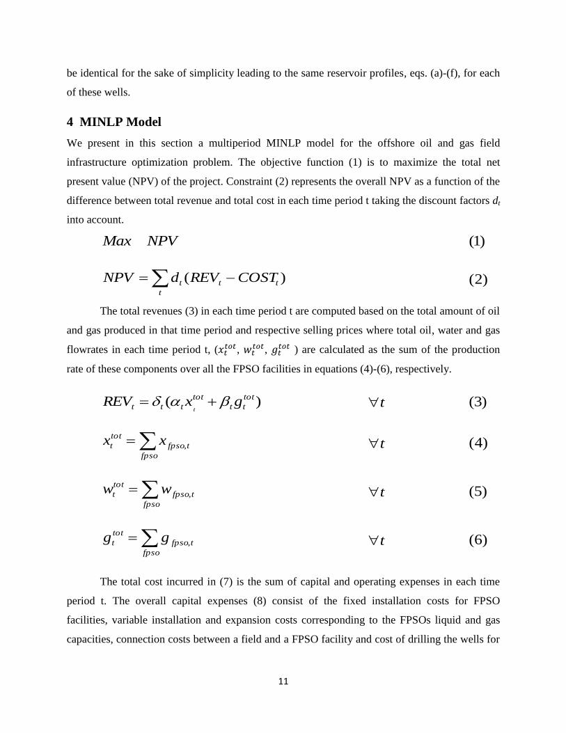
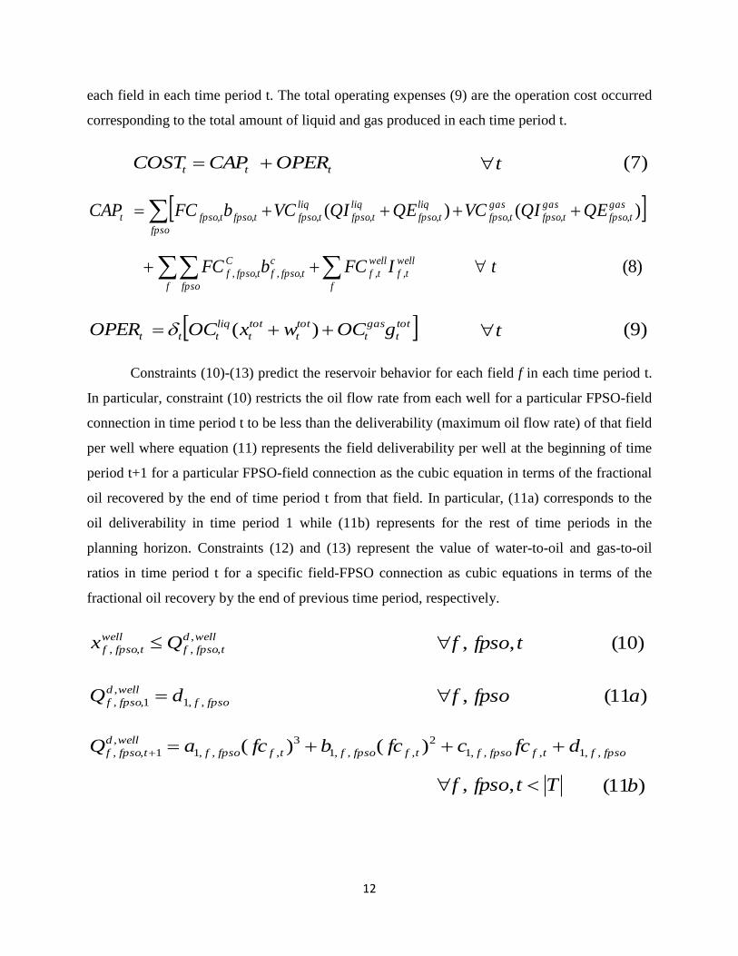
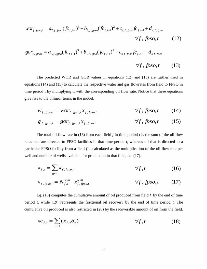
When oil is extracted from a reservoir oil deliverability, water-to-oil ratio (WOR) and

gas-to-oil ratio (GOR) change nonlinearly as a function of the cumulative oil recovered from the

reservoir. The initial oil and gas reserves in the reservoirs, as well as the relationships for WOR

and GOR in terms of fractional recovery (fc), are estimated from geologic studies. Figures 1 (a) –

(c) represent the oil deliverability from a field per well, WOR and GOR versus fractional oil

recovered from that field. We can see from these figures that there are different nonlinear field

profiles for different field-FPSO connections to account for the variations in the flows for each

of these possible connections.

The maximum oil flowrate (field deliverability) per well can be represented as a 3rd

order

polynomial equation (a) in terms of the fractional recovery. Furthermore, the actual oil flowrate

(xf ) from each of the wells is restricted by both the field deliverability , (b), and facility

capacity. We assume that there is no need for enhanced recovery, i.e., no need for injection of

gas or water into the reservoir. The oil produced from the wells (xf ) contains water and gas and

their relative rates depend on water-to-oil ratio (worf) and gas-to-oil ratio (gorf) that are

approximated using 3rd

order polynomial functions in terms of fractional oil recovered (eqs. (c)-

(d)). The water and gas flow rates can be calculated by multiplying the oil flowrate (xf ) with

water-to-oil ratio and gas-to-oil ratio as in eqs. (e) and (f), respectively. Note that the reason for

considering fractional oil recovery compared to cumulative amount of oil was to avoid numerical

difficulties that could arise due to very small magnitude of the polynomial coefficients in that

case.

0

0.5

1

1.5

2

2.5

3

0 0.5 1

WO

R (

stb

/stb

)

fc

Water-oil-ratio

wor(F1-FPSO1)

wor(F1-FPSO2)

0

0.2

0.4

0.6

0.8

1

1.2

0 0.5 1

GO

R (

kscf

/stb

)

fc

Gas-oil-ratio

gor(F1-FPSO1)

gor(F1-FPSO2)

Figure 1: Nonlinear Reservoir Characteristics for field (F1) for 2 FPSO facilities (FPSO 1 and 2)

(b) Water to oil ratio for field (F1) (b) Gas to oil ratio for field (F1)

9

1,1

2

,1

3

,,1 )()( dfccfcbfcaQ fffftff

d

f

f (a)

d

ff Qx

f (b)

ffffffff dfccfcbfcawor ,2,2

2

,2

3

,2 )()(

f (c)

ffffffff dfccfcbfcagor ,3,3

2

,3

3

,3 )()(

f (d)

fff xworw

f (e)

fff xgorg

f (f)

In Appendix A we derive the polynomial equations for the cumulative water and

cumulative gas produced as a function of fractional recovery using equations (c) and (d),

respectively, in order to avoid the bilinear terms (e)-(f) that are required in the model based on

the above reservoir equations. In the next section, we give a formal description of the oilfield

development problem considered in the paper that is formulated as an MINLP problem in the

subsequent section.

3 Problem Statement

Given is a typical offshore oilfield infrastructure consisting of a set of oil fields F = {1,2,…f}

available for producing oil using a set of FPSO (Floating, Production, Storage and Offloading)

facilities, FPSO = {1,2,…fpso}, (see Fig. 2). To produce oil from a field, it must be connected to a

FPSO facility that can process the produced oil, store and offload it to the other tankers.

FPSO FPSO

Field

Field

Field

Field

Figure 2: Typical Offshore Oilfield Infrastructure Representation

Total Oil/Gas

Production

10

We assume that the location of each FPSO facility and its possible connections to the

given fields are known (Figure 2). Notice that each FPSO facility can be connected to more than

one field to produce oil while a field can only be connected to a single FPSO facility. There can

be a significant amount of water and gas that comes out with the oil during the production

process that needs to be considered while planning for FPSO capacity installations and

expansions. The water is usually re-injected after separation from the oil while the gas can be

sold in the market. In this case for simplicity we do not consider water or gas re-injection i.e.

natural depletion of the reserves.

To develop and operate such a complex and capital intensive offshore oilfield

infrastructure, we have to make the optimum investment and operation decisions to maximize the

NPV considering a long-term planning horizon. The planning horizon is discretized into a

number of time periods t, typically each with 1 year of duration. Investment decisions in each

time period t include which FPSO facilities should be installed or expanded, and their respective

installation or expansion capacities for oil, liquid and gas, which fields should be connected to

which FPSO facility, and the number of wells that should be drilled in a particular field f given

the restrictions on the total number of wells that can be drilled in each time period t over all the

given fields. Operating decisions include the oil/gas production rates from each field f in each

time period t. It is assumed that all the installation and expansion decisions occur at the

beginning of each time period t, while operation takes place throughout the time period. There is

a lead time of l1 years for each FPSO facility initial installation and a lead time of l2 years for the

expansion of an earlier installed FPSO facility. Once installed, we assume that the oil, liquid (oil

and water) and gas capacities of a FPSO facility can be expanded only once.

Field deliverability, i.e. maximum oil flowrate from a field, WOR and GOR are

approximated by a cubic equation, while cumulative water produced and cumulative gas

produced from a field are represented by fourth order polynomials in terms of the fractional oil

recovered from that field. Notice that these 4th

order polynomials correspond to the integration of

the cubic equations for WOR and GOR as explained in Appendix A. The motivation for using

polynomials for cumulative water produced and cumulative gas produced as compared to WOR

and GOR is to avoid bilinear terms in the formulation and to allow converting the resulting

model into an MILP formulation. Furthermore, all the wells in a particular field f are assumed to

11

be identical for the sake of simplicity leading to the same reservoir profiles, eqs. (a)-(f), for each

of these wells.

4 MINLP Model

We present in this section a multiperiod MINLP model for the offshore oil and gas field

infrastructure optimization problem. The objective function (1) is to maximize the total net

present value (NPV) of the project. Constraint (2) represents the overall NPV as a function of the

difference between total revenue and total cost in each time period t taking the discount factors dt

into account.

NPVMax

)1(

)( tt

t

t COSTREVdNPV

)2(

The total revenues (3) in each time period t are computed based on the total amount of oil

and gas produced in that time period and respective selling prices where total oil, water and gas

flowrates in each time period t, ( ,

, ) are calculated as the sum of the production

rate of these components over all the FPSO facilities in equations (4)-(6), respectively.

)( tot

tt

tot

ttt gxREVt

t )3(

fpso

tfpso

tot

t xx ,

t )4(

fpso

tfpso

tot

t ww ,

t )5(

fpso

tfpso

tot

t gg ,

t )6(

The total cost incurred in (7) is the sum of capital and operating expenses in each time

period t. The overall capital expenses (8) consist of the fixed installation costs for FPSO

facilities, variable installation and expansion costs corresponding to the FPSOs liquid and gas

capacities, connection costs between a field and a FPSO facility and cost of drilling the wells for

12

each field in each time period t. The total operating expenses (9) are the operation cost occurred

corresponding to the total amount of liquid and gas produced in each time period t.

ttt OPERCAPCOST

t )7(

)8(

)()(

,,,,,,

,,,,,,,,

tIFCbFC

QEQIVCQEQIVCbFCCAP

f fpso f

well

tf

well

tf

c

tfpsof

C

tfpsof

fpso

gas

tfpso

gas

tfpso

gas

tfpso

liq

tfpso

liq

tfpso

liq

tfpsotfpsotfpsot

tot

t

gas

t

tot

t

tot

t

liq

ttt gOCwxOCOPER )(

t )9(

Constraints (10)-(13) predict the reservoir behavior for each field f in each time period t.

In particular, constraint (10) restricts the oil flow rate from each well for a particular FPSO-field

connection in time period t to be less than the deliverability (maximum oil flow rate) of that field

per well where equation (11) represents the field deliverability per well at the beginning of time

period t+1 for a particular FPSO-field connection as the cubic equation in terms of the fractional

oil recovered by the end of time period t from that field. In particular, (11a) corresponds to the

oil deliverability in time period 1 while (11b) represents for the rest of time periods in the

planning horizon. Constraints (12) and (13) represent the value of water-to-oil and gas-to-oil

ratios in time period t for a specific field-FPSO connection as cubic equations in terms of the

fractional oil recovery by the end of previous time period, respectively.

welld

tfpsof

well

tfpsof Qx ,

,,,,

tfpsof ,,

)10(

fpsof

welld

fpsof dQ ,,1

,

1,,

fpsof ,

)11( a

fpsoftffpsoftffpsoftffpsof

welld

tfpsof dfccfcbfcaQ ,,1,,,1

2

,,,1

3

,,,1

,

1,, )()(

Ttfpsof ,,

)11( b

13

fpsoftffpsoftffpsoftffpsoftfpsof dfccfcbfcawor ,,21,,,2

2

1,,,2

3

1,,,2,, )()(

tfpsof ,, )12(

fpsoftffpsoftffpsoftffpsoftfpsof dfccfcbfcagor ,,31,,,3

2

1,,,3

3

1,,,3,, )()(

tfpsof ,,

)13(

The predicted WOR and GOR values in equations (12) and (13) are further used in

equations (14) and (15) to calculate the respective water and gas flowrates from field to FPSO in

time period t by multiplying it with the corresponding oil flow rate. Notice that these equations

give rise to the bilinear terms in the model.

tfpsoftfpsoftfpsof xworw ,,,,,, tfpsof ,,

)14(

tfpsoftfpsoftfpsof xgorg ,,,,,, tfpsof ,, )15(

The total oil flow rate in (16) from each field f in time period t is the sum of the oil flow

rates that are directed to FPSO facilities in that time period t, whereas oil that is directed to a

particular FPSO facility from a field f is calculated as the multiplication of the oil flow rate per

well and number of wells available for production in that field, eq. (17).

fpso

tfpsoftf xx ,,,

tf ,

)16(

well

tfpsof

well

tftfpsof xNx ,,,,,

tfpsof ,,

)17(

Eq. (18) computes the cumulative amount of oil produced from field f by the end of time

period t, while (19) represents the fractional oil recovery by the end of time period t. The

cumulative oil produced is also restricted in (20) by the recoverable amount of oil from the field.

)(1

,,

t

ftf xxc

tf ,

)18(

14

f

tf

tfREC

xcfc

,

,

tf ,

)19(

ftf RECxc , tf ,

)20(

Eqs. (21)-(23) compute total oil, water and gas flow rates into each FPSO facility,

respectively, in time period t from all the given fields.

f

tfpsoftfpso xx ,,,

tfpso,

)21(

f

tfpsoftfpso ww ,,,

tfpso,

)22(

f

tfpsoftfpso gg ,,,

tfpso,

)23(

There are three types of capacities i.e. for oil, liquid (oil and water) and gas that are used

for modeling the capacity constraints for FPSO facilities. Specifically, Eqs. (24)-(26) restrict the

total oil, liquid and gas flow rates into each FPSO facility to be less than its corresponding

capacity in each time period t respectively. These three different kinds of capacities of a FPSO

facility in time period t are computed by equalities (27)-(29) as the sum of the corresponding

capacity at the end of previous time period t-1, installation capacity at the beginning of time

period t-l1 and expansion capacity at the beginning of time period t-l2. Specifically, the term

in equation (27) represents the oil capacity of a FPSO facility that started to install l1

years earlier and is expected to be ready for production in time period t, to account for the lead

time of l1 years for a FPSO facility installation. The term represents the expansion

decision in the oil capacity of an already installed FPSO facility that is taken l2 years before time

period t, to consider the lead time of l2 years for capacity expansion. Similarly, the corresponding

terms in equations (28) and (29) represent the lead times for liquid and gas capacity installation

or expansion, respectively. Notice that due to one installation and expansion of a FPSO facility,

and

can have non-zero values only once in the planning horizon while

can be non-zero in the multiple time periods.

15

oil

tfpsotfpso Qx ,, tfpso,

)24(

liq

tfpsotfpsotfpso Qwx ,,,

tfpso,

)25(

gas

tfpsotfpso Qg ,, tfpso,

)26(

oil

ltfpso

oil

ltfpso

oil

tfpso

oil

tfpso QEQIQQ21 ,,1,,

tfpso,

)27(

liq

ltfpso

liq

ltfpso

liq

tfpso

liq

tfpso QEQIQQ21 ,,1,,

tfpso,

)28(

gas

ltfpso

gas

ltfpso

gas

tfpso

gas

tfpso QEQIQQ21 ,,1,,

tfpso,

)29(

Inequalities (30) and (31) restrict the installation and expansion of a FPSO facility to take

place only once, respectively, while inequality (32) states that the connection between a FPSO

facility and a field can be installed only once during the whole planning horizon. Inequality (33)

ensures that a field can be connected to at most one FPSO facility in each time period t, while

(34) states that at most one FPSO-field connection is possible for a field f during the entire

planning horizon T due to engineering considerations. Constraints (35) and (36) state that the

expansion in the capacity of a FPSO facility and the connection between a field and a FPSO

facility, respectively, in time period t can occur only if that FPSO facility has already been

installed by that time period.

1, Tt

tfpsob

fpso

)30(

1,

Tt

ex

tfpsob

fpso

)31(

1,,

Tt

c

tfpsofb

fpsof ,

)32(

1,,

fpso

c

tfpsofb

tf ,

)33(

Tt fpso

c

tfpsofb 1,,

f

)34(

16

t

fpso

ex

tfpso bb1

,,

tfpso,

)35(

t

fpso

c

tfpsof bb1

,,,

tfpsof ,,

)36(

Inequality (37) states that the oil flow rate per well from a field f to a FPSO facility in

time period t will be zero if that FPSO-field connection is not available in that time period.

Notice that equations (17) and (37) ensure that for production from a field in time period t there

must be a field-FPSO connection and at-least one well available in that field at the beginning of

time period t. Constraints (38)-(43) are the upper-bounding constraints on the installation and

expansion capacities for FPSO facilities in time period t corresponding to the three different

kinds of capacities mentioned earlier.

t

c

fpsof

oilwell

fpsof

well

tfpsof bUx1

,,

,

,,,

tfpsof ,,

)37(

tfpso

oil

fpso

oil

tfpso bUQI ,, tfpso,

)38(

tfpso

liq

fpso

liq

tfpso bUQI ,, tfpso,

)39(

tfpso

gas

fpso

gas

tfpso bUQI ,, tfpso,

)40(

ex

tfpso

oil

fpso

oil

tfpso bUQE ,, tfpso,

)41(

ex

tfpso

liq

fpso

liq

tfpso bUQE ,, tfpso,

)42(

exp

,, tfpso

gas

fpso

gas

tfpso bUQE

tfpso,

)43(

The additional restrictions on the oil, liquid and gas expansion capacities of FPSO

facilities, (44)-(46), come from the fact that these expansion capacities should be less than a

certain fraction (µ) of the initial built capacities, respectively. Notice that available capacitates

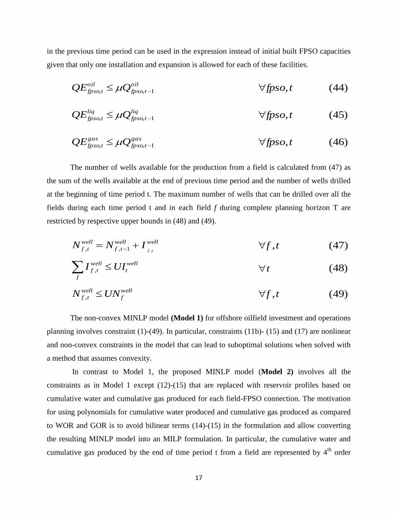
17

in the previous time period can be used in the expression instead of initial built FPSO capacities

given that only one installation and expansion is allowed for each of these facilities.

oil

tfpso

oil

tfpso QQE 1,,

tfpso,

)44(

liq

tfpso

liq

tfpso QQE 1,,

tfpso,

)45(

gas

tfpso

gas

tfpso QQE 1,,

tfpso,

)46(

The number of wells available for the production from a field is calculated from (47) as

the sum of the wells available at the end of previous time period and the number of wells drilled

at the beginning of time period t. The maximum number of wells that can be drilled over all the

fields during each time period t and in each field f during complete planning horizon T are

restricted by respective upper bounds in (48) and (49).

wellwell

tf

well

tf tfINN

,1,, tf ,

)47(

well

t

f

well

tf UII ,

t

)48(

well

f

well

tf UNN , tf ,

)49(

The non-convex MINLP model (Model 1) for offshore oilfield investment and operations

planning involves constraint (1)-(49). In particular, constraints (11b)- (15) and (17) are nonlinear

and non-convex constraints in the model that can lead to suboptimal solutions when solved with

a method that assumes convexity.

In contrast to Model 1, the proposed MINLP model (Model 2) involves all the

constraints as in Model 1 except (12)-(15) that are replaced with reservoir profiles based on

cumulative water and cumulative gas produced for each field-FPSO connection. The motivation

for using polynomials for cumulative water produced and cumulative gas produced as compared

to WOR and GOR is to avoid bilinear terms (14)-(15) in the formulation and allow converting

the resulting MINLP model into an MILP formulation. In particular, the cumulative water and

cumulative gas produced by the end of time period t from a field are represented by 4th

order

18

polynomial equations (50) and (51), respectively, in terms of fractional oil recovery by the end of

time period t. Notice that these 4th

order polynomials (50) and (51) correspond to the cubic

equations for WOR and GOR, respectively, that are derived in Appendix A.

tffpsoftffpsoftffpsoftffpsof

wc

tfpsof fcdfccfcbfcaQ ,,,2

2

,,,2

3

,,,2

4

,,,2,, )()()(

tfpsof ,,

)50(

tffpsoftffpsoftffpsoftffpsof

gc

tfpsof fcdfccfcbfcaQ ,,,3

2

,,,3

3

,,,3

4

,,,3,, )()()(

tfpsof ,,

)51(

Notice that variables and

will be non-zero in equations (50) and (51)

if is non-zero even though that particular field-FPSO connection is not present. Therefore,

and

represent dummy variables in equations (50) and (51) instead of actual

cumulative water ( and cumulative gas recoveries due to the fact that only

those cumulative water and cumulative gas produced can be non-zero that has the specific FPSO-

field connection present in that time period t. Therefore, we introduce constraints (52)-(55) to

equate the actual cumulative water produced, , for a field-FPSO connection by the end

of time period t to the corresponding dummy variable only if that field-FPSO

connection is present in time period t else is set to zero. Similarly, constraints (56)-(59)

equate the actual cumulative gas produced , to the dummy variable

only if

that field-FPSO connection is present in time period t, otherwise it is set to zero. and

correspond to maximum amount of cumulative water and gas that can be produced for a

particular field and FPSO connection during the entire planning horizon, respectively. Note that

the motivation for using dummy variables ( and

) for cumulative water and

cumulative gas flows in equations (50)-(51) followed by big-M constraints (52)-(59), instead of

using disaggregated variables for the fractional recovery in equations (50)-(51) directly, was to

avoid large number of SOS1 variables while MILP reformulation of this model as explained in

the next section.

19

t

c

fpsof

wc

fpsof

wc

tfpsoftfpsof bMQwc1

,,,,,,, )1(

tfpsof ,,

)52(

t

c

fpsof

wc

fpsof

wc

tfpsoftfpsof bMQwc1

,,,,,,, )1(

tfpsof ,,

)53(

t

c

fpsof

wc

fpsoftfpsof bMwc1

,,,,,

tfpsof ,,

)54(

t

c

fpsof

wc

fpsoftfpsof bMwc1

,,,,,

tfpsof ,,

)55(

t

c

fpsof

gc

fpsof

gc

tfpsoftfpsof bMQgc1

,,,,,,, )1(

tfpsof ,,

)56(

t

c

fpsof

gc

fpsof

gc

tfpsoftfpsof bMQgc1

,,,,,,, )1(

tfpsof ,,

)57(

t

c

fpsof

gc

fpsoftfpsof bMgc1

,,,,,

tfpsof ,,

)58(

t

c

fpsof

gc

fpsoftfpsof bMgc1

,,,,,

tfpsof ,,

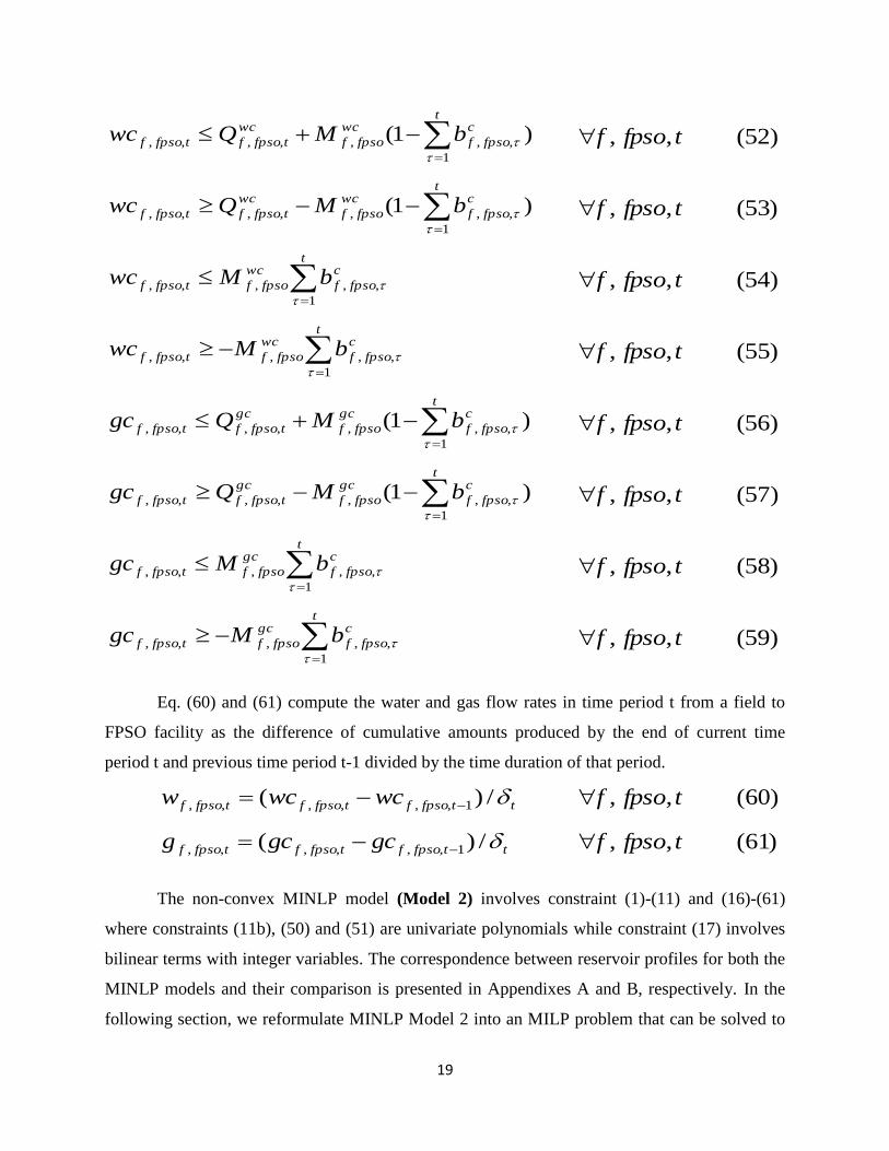
)59(

Eq. (60) and (61) compute the water and gas flow rates in time period t from a field to

FPSO facility as the difference of cumulative amounts produced by the end of current time

period t and previous time period t-1 divided by the time duration of that period.

ttfpsoftfpsoftfpsof wcwcw /)( 1,,,,,,

tfpsof ,,

)60(

ttfpsoftfpsoftfpsof gcgcg /)( 1,,,,,,

tfpsof ,,

)61(

The non-convex MINLP model (Model 2) involves constraint (1)-(11) and (16)-(61)

where constraints (11b), (50) and (51) are univariate polynomials while constraint (17) involves

bilinear terms with integer variables. The correspondence between reservoir profiles for both the

MINLP models and their comparison is presented in Appendixes A and B, respectively. In the

following section, we reformulate MINLP Model 2 into an MILP problem that can be solved to

20

global optimality in an effective way. Notice that due to the presence of bilinear terms in

equations (14) and (15), Model 1 cannot be reformulated into an MILP problem.

5 MILP Reformulation

The nonlinearites involved in Model 2 include univariate polynomials (11b), (50), (51) and

bilinear equations (17). In this section, we reformulate this model into an MILP model, Model 3

using piecewise linearization and exact linearization techniques that can give the global solution

of the resulting approximate problem.

To approximate the 3rd

and 4th

order univariate polynomials (11b), (50) and (51) SOS1

variables are introduced to select the adjacent points l-1 and l for interpolation over an

interval l. Constraints (62)-(65) represent the piecewise linear approximation for the fractional

recovery and corresponding oil deliverability, cumulative water and cumulative gas produced for

a field in each time period t, respectively, where ̃ , ̃

, ̃

and ̃

are the

values of the corresponding variables at point l used in linear interpolation based on the reservoir

profiles (11b), (50) and (51). Note that only variables are sufficient to approximate the

constraints (11b), (50) and (51) by selecting a specific value of the fractional recovery for each

field in each time period t that applies to all possible field-FPSO connections for that field. This

avoids the requirement of a large number of SOS1 variables and resulting increase in the solution

times that would have been required in the case if constraints (50) and (51) were represented in

terms of the disaggregated variables for fractional recovery in Model 2.

n

l

ll

tftf cffc1

,,

~

tf ,

)62(

n

l

lwelld

fpsof

l

tf

welld

tfpsof QQ1

,,

,,

,

1,,

~

Ttfpsof ,,

)63(

n

l

lwc

fpsof

l

tf

wc

tfpsof QQ1

,

,,,,

~

tfpsof ,,

)64(

n

l

lgc

fpsof

l

tf

gc

tfpsof QQ1

,

,,,,

~

tfpsof ,,

)65(

21

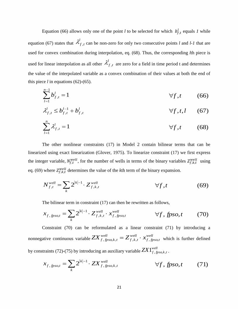
Equation (66) allows only one of the point l to be selected for which equals 1 while

equation (67) states that l

tf , can be non-zero for only two consecutive points l and l-1 that are

used for convex combination during interpolation, eq. (68). Thus, the corresponding lth piece is

used for linear interpolation as all other l

tf , are zero for a field in time period t and determines

the value of the interpolated variable as a convex combination of their values at both the end of

this piece l in equations (62)-(65).

1

1

, 1n

l

l

tfb

tf ,

)66(

l

tf

l

tf

l

tf bb ,

1

,,

ltf ,,

)67(

n

l

l

tf

1

, 1

tf ,

)68(

The other nonlinear constraints (17) in Model 2 contain bilinear terms that can be

linearized using exact linearization (Glover, 1975). To linearize constraint (17) we first express

the integer variable, , for the number of wells in terms of the binary variables

using

eq. (69) where determines the value of the kth term of the binary expansion.

k

well

tkf

kwell

tf ZN ,,

1

, 2

tf ,

)69(

The bilinear term in constraint (17) can then be rewritten as follows,

k

well

tfpsof

well

tkf

k

tfpsof xZx ,,,,

1

,, 2

tfpsof ,,

)70(

Constraint (70) can be reformulated as a linear constraint (71) by introducing a

nonnegative continuous variablewell

tfpsof

well

tkf

well

tkfpsof xZZX ,,,,,,, which is further defined

by constraints (72)-(75) by introducing an auxiliary variablewell

tkfpsofZX ,,,1 .

k

well

tkfpsof

k

tfpsof ZXx ,,,

1

,, 2

tfpsof ,,

)71(

22

well

tfpsof

well

tkfpsof

well

tkfpsof xZXZX ,,,,,,,, 1

tkfpsof ,,,

)72(

well

tkf

well

fpsof

well

tkfpsof ZUZX ,,,,,,

tkfpsof ,,,

)73(

)1(1 ,,,,,,

well

tkf

well

fpsof

well

tkfpsof ZUZX

tkfpsof ,,,

)74(

01,0 ,,,,,, well

tkfpsof

well

tkfpsof ZXZX

tkfpsof ,,,

)75(

The reformulated MILP Model 3 involves constraints (1)-(10), (11a), (16), (18)-(69) and

(71)-(75) which are linear and mixed-integer linear constraints and allow to solve this

approximate problem to global optimality using standard mixed-integer linear programming

solvers.

Remarks

The previous two sections present a multiperiod MINLP model for the oilfield investment

and operations planning problem for long-term planning horizon and its reformulation as an

MILP model using linearization techniques. The MINLP models involve non-convexities and

can yield suboptimal solutions when using an MINLP solver that relies on convexity

assumptions, while the reformulated MILP model is guaranteed to be solved to global optimality

using linear programming based branch and cut methods. However, given the difficulties

involved in solving large scale instances of the MINLP and MILP models, especially due to the

large number of binary variables, we extend these formulations by reducing the number of the

binary variables. The next section describes the proposed procedure for binary reduction for

MINLP and MILP formulations.

6 Reduced MINLP and MILP models

Due to the potential computational expense of solving the large scale MINLP and MILP models

presented in the previous sections, we further reformulate them by removing many binary

variables, namely . These binary variables represent the timing of the connections

between fields and FPSOs and are used for discounting the connection cost in the objective

function along with some logic constraints in the proposed models. The motivation for binary

reduction comes from the fact that in the solution of these models the connection cost is only ~2-

3% of the total cost, and hence, this cost can be removed from the objective function as its exact

23

discounting does not has a significant impact on the optimal solution. In particular, we propose

to drop the index t from , which results in a significant decrease in the number of binary

variables (~33% reduction) and the solution time can be improved significantly for both the

MINLP and MILP formulations.

Therefore, to formulate the reduced models that correspond to Model 2 and 3 we use the

binary variables to represent the connection between field and FPSOs instead of using

which results in a significant decrease in the number of binary variables in the model.

As an example for a field with 5 possible FPSO connections and 20 years planning horizon the

number of binary variables required can be reduced from 100 to 5. The connection cost term in

the objective function (8) is also removed as explained above yielding constraint (76).

Moreover, some of the constraints in the previous MINLP and MILP models that involve binary

variables are reformulated to be valid for

based reduced model, i.e. constraints

(77)-(87). Notice that constraints (87) and (17) ensure that the oil flow rate from a field to FPSO

facility in time period t, , will be non-zero only if that particular field-FPSO connection

is installed and there is atleast one well available in that field for production in time period t, i.e.

equals 1 and

is non-zero, otherwise is set to zero. Moreover, it may be

possible that variable can take non-zero value in equation (87) if

equals 1 even

though there is no well available in that field in time period t, but this will not have any effect on

the solution given that the fractional recovery from a field and other calculations/constraints in

the model are based on the actual amount of oil produced from the field, i.e. variable

which is still zero in this case. Therefore, variable can be considered as a dummy

variable in the reduced model.

)76(

)()(

,,

,,,,,,,,

tIFC

QEQIVCQEQIVCbFCCAP

f

well

tf

well

tf

fpso

gas

tfpso

gas

tfpso

gas

tfpso

liq

tfpso

liq

tfpso

liq

tfpsotfpsotfpsot

)1( ,,,,,,

R

fpsof

wc

fpsof

wc

tfpsoftfpsof bMQwc

tfpsof ,,

)77(

)1( ,,,,,,

R

fpsof

wc

fpsof

wc

tfpsoftfpsof bMQwc

tfpsof ,,

)78(

24

R

fpsof

wc

fpsoftfpsof bMwc ,,,,

tfpsof ,,

)79(

R

fpsof

wc

fpsoftfpsof bMwc ,,,,

tfpsof ,,

)80(

)1( ,,,,,,

R

fpsof

gc

fpsof

gc

tfpsoftfpsof bMQgc

tfpsof ,,

)81(

)1( ,,,,,,

R

fpsof

gc

fpsof

gc

tfpsoftfpsof bMQgc

tfpsof ,,

)82(

R

fpsof

gc

fpsoftfpsof bMgc ,,,,

tfpsof ,,

)83(

R

fpsof

gc

fpsoftfpsof bMgc ,,,,

tfpsof ,,

)84(

1,

fpso

R

fpsofb

f

)85(

t

fpso

R

fpsof bb1

,,

tfpsof ,,

)86(

R

fpsof

oilwell

fpsof

well

tfpsof bUx ,

,

,,,

tfpsof ,,

)87(

The non-convex MINLP Model 2-R for offshore oilfield investment and operations

planning after binary reduction involves constraints (1)-(7), (9)-(11), (16)-(31), (35), (38)-(51),

(60)-(61) and (76)-(87). The reformulated MILP Model 3-R after binary reduction involves

constraints (1)-(7), (9)-(10), (11a), (16), (18)-(31), (35), (38)-(51), (60)-(69) and (71)-(87) which

are linear and mixed-integer linear constraints. Similarly, Model 1-R corresponds to the non-

convex MINLP model, which is based on WOR and GOR expression after binary reduction as

described above.

The resulting reduced models with fewer binaries can be solved much more efficiently as

compared to the original models. To calculate the discounted cost of connections between field

and FPSOs that corresponds to the reduced model solution, we use the well installation schedule

from the optimal solution of reduced models to find the Field-FPSO connection timing and

subtract the corresponding discounted connection cost from the optimal NPV of the reduced

model. The resulting NPV represents the optimal NPV of the original models in case connection

costs are relatively small.

25

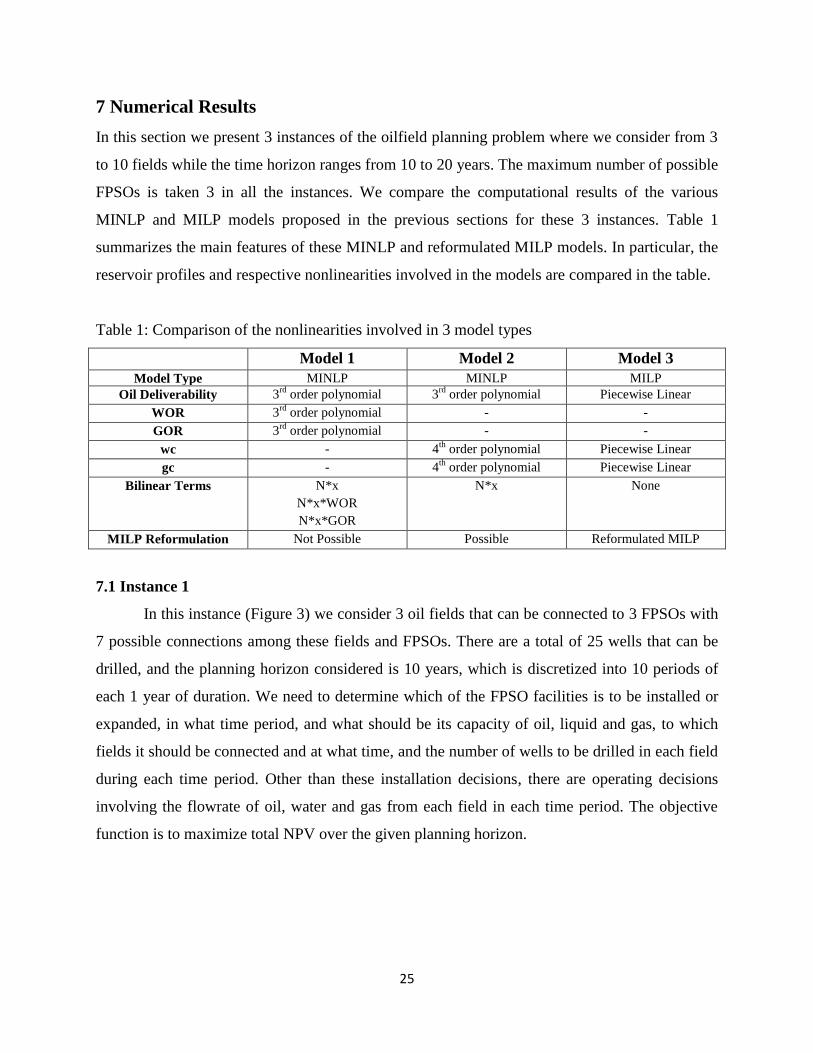
7 Numerical Results

In this section we present 3 instances of the oilfield planning problem where we consider from 3

to 10 fields while the time horizon ranges from 10 to 20 years. The maximum number of possible

FPSOs is taken 3 in all the instances. We compare the computational results of the various

MINLP and MILP models proposed in the previous sections for these 3 instances. Table 1

summarizes the main features of these MINLP and reformulated MILP models. In particular, the

reservoir profiles and respective nonlinearities involved in the models are compared in the table.

Table 1: Comparison of the nonlinearities involved in 3 model types

Model 1 Model 2 Model 3

Model Type MINLP MINLP MILP

Oil Deliverability 3rd

order polynomial 3rd

order polynomial Piecewise Linear

WOR 3rd

order polynomial - -

GOR 3rd

order polynomial - -

wc - 4th

order polynomial Piecewise Linear

gc - 4th

order polynomial Piecewise Linear

Bilinear Terms N*x

N*x*WOR

N*x*GOR

N*x None

MILP Reformulation Not Possible Possible Reformulated MILP

7.1 Instance 1

In this instance (Figure 3) we consider 3 oil fields that can be connected to 3 FPSOs with

7 possible connections among these fields and FPSOs. There are a total of 25 wells that can be

drilled, and the planning horizon considered is 10 years, which is discretized into 10 periods of

each 1 year of duration. We need to determine which of the FPSO facilities is to be installed or

expanded, in what time period, and what should be its capacity of oil, liquid and gas, to which

fields it should be connected and at what time, and the number of wells to be drilled in each field

during each time period. Other than these installation decisions, there are operating decisions

involving the flowrate of oil, water and gas from each field in each time period. The objective

function is to maximize total NPV over the given planning horizon.

26

The problem is solved using DICOPT 2x-C solver for Models 1 and 2, and CPLEX 12.2

for Model 3. These models were implemented in GAMS 23.6.3 and run on Intel Core i7

machine. The optimal solution of this problem that corresponds to Model 2, suggests installing

only FPSO 3 with a capacity of 300 kstb/d, 420.01 kstb/d and 212.09 MMSCF/d for oil, liquid

and gas, respectively, at the beginning of time period 1. All the three fields are connected to this

FPSO facility at time period 4 when installation of the FPSO facility is completed and a total of

20 wells are drilled in these 3 fields in that time period to start production. One additional well is

also drilled in field 3 in time period 5 and there are no expansions in the capacity of FPSO

facility. The total NPV of this project is $6912.04 M.

Table 2: Performance of various solvers with Model 1 and 2 for Instance 1

Model 1 Model 2

Constraints 1,357 1,997

Continuous Var. 1,051 1,271

Discrete Var. 151 151

Solver

Optimal NPV

(million$)

Time (s) Optimal NPV

(million$)

Time (s)

DICOPT 6980.92 3.56 6912.04 3.07

SBB 7038.26 211.53 6959.06 500.64

BARON 6983.65 >36,000 6919.28 >36,000

Table 2 compares the computational results of Model 1 and 2 for this instance with

various MINLP solvers. We can observe from these results that DICOPT performs best among

FPSO 1 FPSO 3

Field 1

Field 3

Field 2

Figure 3: Instance 1 (3 Fields, 3 FPSO, 10 years) for oilfield problem

Total Oil/Gas

Production

FPSO 2

27

all the MINLP solvers in terms of computational time, while solving directly both Models 1 and

2. The number of OA iterations required is approximately 3-4 in both cases, and solving Model 2

is slightly easier than solving Model 1 directly with this solver. However, the solutions obtained

are not guaranteed to be the global solution. SBB is also reasonable in terms of solution quality

but it takes much longer time to solve. BARON can in principle find the global optimum solution

to models 1 and 2, but it is very slow and takes more than 36,000s to be within ~23% and ~10%

of optimality gap for these models, respectively. Note that we use the DICOPT solution to

initialize in this case, but BARON could only provide a slightly better solution (6983.65 vs.

6980.92 and 6919.28 vs. 6912.04) than DICOPT in more than 10 hours for both the cases.

The performance of Models 1 and 2 are compared before and after reducing the binary

variables for connection, i.e. Models 1-R and 2-R, in Table 3. There is one third reduction in the

number of binary variables for both models. It can also be seen that there is a significant decrease

in the solution time after binary reduction (for e.g. 1.55s vs. 3.56s for Model 1). Moreover, the

reduced models also yield better local solutions too for both the MINLP formulations. Notice

that these MINLP Models are solved with DICOPT here for comparison as it is much faster as

compared to other solvers as seen from the previous results.

The MILP Model 3 and its binary reduction Model 3-R that are formulated from Model 2

and Model 2-R, respectively, solved with CPLEX 12.2 and results in Table 3 show the

significant reduction in the solution time after binary reduction (6.55s vs. 37.03s) while both the

models give same optimal NPV i.e. $7030.90M. Notice that these approximate MILP models are

solved upto global optimality in few seconds while global solution of the original MINLP

formulations is much expensive to obtain. Although the higher the number of points for the

approximate MILP model the better will be the solution quality, but we found that beyond 5

points for the piecewise approximation there was not much significant change in the optimal

solution, while it led to large increases in the solution time due to increase in the SOS1 variables

in the model. Therefore we use 5 point estimates for piecewise linearization to formulate Model

3 and 3-R for all the instances.

28

*Model 1 and 2 solved with DICOPT 2x-C, Model 3 solved with CPLEX 12.2

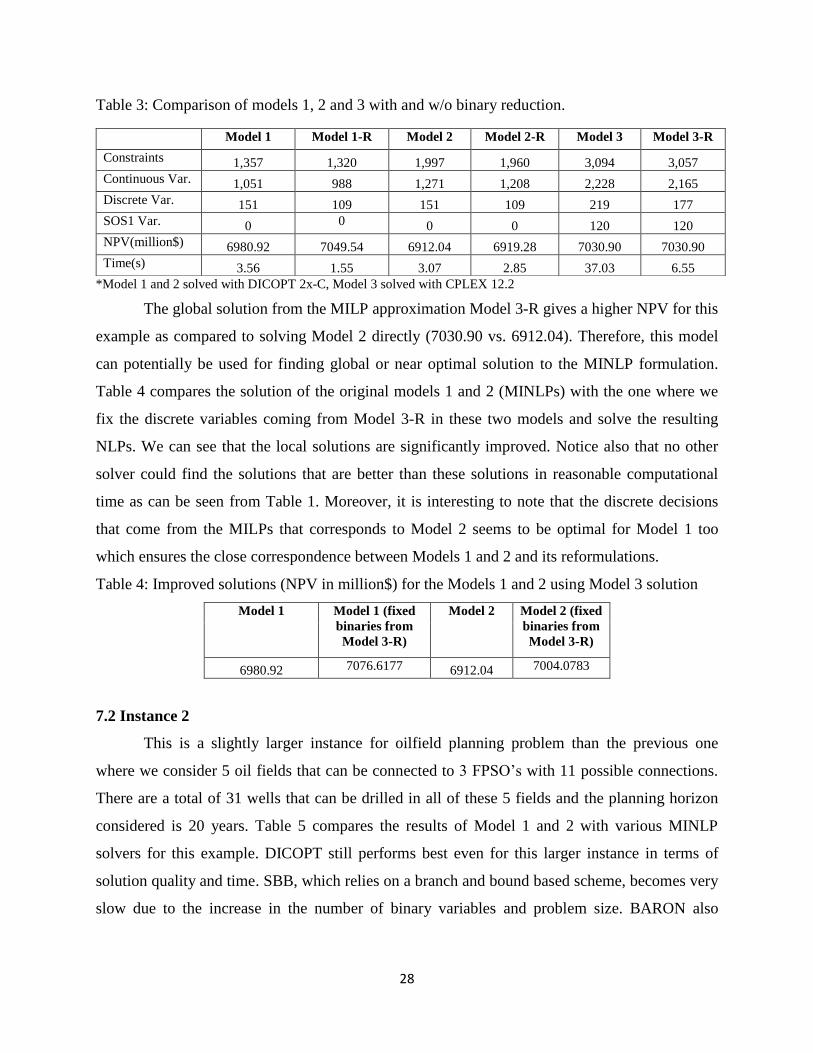
The global solution from the MILP approximation Model 3-R gives a higher NPV for this

example as compared to solving Model 2 directly (7030.90 vs. 6912.04). Therefore, this model

can potentially be used for finding global or near optimal solution to the MINLP formulation.

Table 4 compares the solution of the original models 1 and 2 (MINLPs) with the one where we

fix the discrete variables coming from Model 3-R in these two models and solve the resulting

NLPs. We can see that the local solutions are significantly improved. Notice also that no other

solver could find the solutions that are better than these solutions in reasonable computational

time as can be seen from Table 1. Moreover, it is interesting to note that the discrete decisions

that come from the MILPs that corresponds to Model 2 seems to be optimal for Model 1 too

which ensures the close correspondence between Models 1 and 2 and its reformulations.

Table 4: Improved solutions (NPV in million$) for the Models 1 and 2 using Model 3 solution

Model 1

Model 1 (fixed

binaries from

Model 3-R)

Model 2 Model 2 (fixed

binaries from

Model 3-R)

6980.92 7076.6177 6912.04 7004.0783

7.2 Instance 2

This is a slightly larger instance for oilfield planning problem than the previous one

where we consider 5 oil fields that can be connected to 3 FPSO’s with 11 possible connections.

There are a total of 31 wells that can be drilled in all of these 5 fields and the planning horizon

considered is 20 years. Table 5 compares the results of Model 1 and 2 with various MINLP

solvers for this example. DICOPT still performs best even for this larger instance in terms of

solution quality and time. SBB, which relies on a branch and bound based scheme, becomes very

slow due to the increase in the number of binary variables and problem size. BARON also

Model 1 Model 1-R Model 2 Model 2-R Model 3 Model 3-R

Constraints 1,357 1,320 1,997 1,960 3,094 3,057

Continuous Var. 1,051 988 1,271 1,208 2,228 2,165

Discrete Var. 151 109 151 109 219 177

SOS1 Var. 0 0 0 0 120 120

NPV(million$) 6980.92 7049.54 6912.04 6919.28 7030.90 7030.90

Time(s) 3.56 1.55 3.07 2.85 37.03 6.55

Table 3: Comparison of models 1, 2 and 3 with and w/o binary reduction.

29

becomes expensive to solve this larger instance and could not improve the DICOPT solution that

is used for its initialization for both the cases in more than 10 hours.

Table 5: Comparison of various models and solvers for Instance 2

Model 1 Model 2

Constraints 3,543 5,543

Continuous Var. 2,781 3,461

Discrete Var. 477 477

Solver Optimal NPV

(million$)

Time (s) Optimal NPV

(million$)

Time (s)

DICOPT 11412.48 58.53 11204.86 18.43

SBB 11376.57 1057.68 11222.34 3309.73

BARON 11412.48 >36,000 11204.86 >36,000

There are significant improvements in computational times for Model 1 and 2 after

binary reduction as can be seen in Table 6 (5.69s vs. 58.53s and 9.92s vs. 18.43s). Moreover,

there are possibilities to find even better local solution too from the reduced model as in the case

of Model 2. The reduced models (Model 1-R and 2-R) should yield the same optimal solutions as

the original models (Model 1 and 2), respectively, for small connection costs but there are slight

differences in the NPV values reported in Table 6 as these models are solved here with DICOPT

that gives the local solutions. The reformulated MILP after binary reduction Model 3-R becomes

slightly expensive to solve as compared to finding local solutions for the original MINLP

models, but the solution obtained in this case is the global one (within 2% optimality tolerance).

Notice that the MILP solutions can be either lower (instance 1) or higher (instance 2) than the

global optimal for MINLP models as these involves approximations of oil deliverability,

cumulative water and cumulative gas produced all three functions and the resulting MILP could

over or underestimate the original NPV function. We do not present the result of Model 3 here as

it gives the same NPV as Model 3-R but at much higher computational expense since a larger

number of binary variables is involved in the model. Note that some of the binary variables are

pre-fixed in all of the models considered based on the earliest installation time of the FPSO

facilities and corresponding limitations on the FPSO expansions, field-FPSO connections and

drilling of the wells in the fields that improves the computational performance of these models.

30

Table 6: Comparison of models 1, 2 and 3 with and w/o binary reduction

Model 1 Model 1-R Model 2 Model 2-R Model 3-R

Constraints 3,543 3,432 5,543 5,432 8,663

Continuous Var. 2,781 2,572 3,461 3,252 6,103

Discrete Var. 477 301 477 301 451

SOS1 Var. 0 0 0 0 400

NPV(million$) 11412.48 11335.01 11204.86 11294.82 11259.61

Time(s) 58.53 5.69 18.43 9.92 871.80

*Model 1 and 2 solved with DICOPT 2x-C, Model 3 solved with CPLEX 12.2

The solution of Model 3-R can also be used to fix discrete variables in the MINLPs to

obtain near optimal solutions to the original problem as done for instance 1. Table 7 presents the

solutions of the NLPs obtained after fixing binary decisions and show that none of the solver in

Table 5 could provide better NPV values than this case. Overall, we can say that the results for

this larger instance also show similar trends as what is observed for instance 1.

Table 7: Improved solutions (NPV in million$) for Models 1 and 2 using Model 3-R solution

Model 1 Model 1 (fixed

binaries from

Model 3-R)

Model 2 Model 2 (fixed

binaries from

Model 3-R)

11412.48 11412.48 11204.86 11356.31

7.3 Instance 3

In this instance we consider 10 oil fields (Figure 4) that can be connected to 3 FPSOs

with 23 possible connections. There are a total of 84 wells that can be drilled in all of these 10

fields and the planning horizon considered is 20 years.

Figure 4: Instance 3 (10 Fields, 3 FPSO, 20 years) for oilfield problem

31

The optimal solution of this problem that corresponds to Model 2-R solved with DICOPT

2x-C, suggests to install all the 3 FPSO facilities in the first time period with their respective

liquid (Figure 5-a) and gas (Figure 5-b) capacities. These FPSO facilities are further expanded in

future when more fields come online or liquid/gas flow rates increases as can be seen from these

figures.

After initial installation of the FPSO facilities by the end of time period 3, these are

connected to the various fields to produce oil in their respective time periods for coming online

as indicated in Figure 6. The well installation schedule for these fields Figure 7 ensures that the

maximum number of wells drilling limit and maximum potential wells in a field are not violated

in each time period t. We can observe from these results that most of the installation and

expansions are in the first few time periods of the planning horizon.

0

100

200

300

400

500

600

700

800

1 3 5 7 9 11 13 15 17 19

Q

liq (

kstb

/d)

Year

Liquid Capacity

fpso1

fpso2

fpso3

0

50

100

150

200

250

300

350

400

1 3 5 7 9 11 13 15 17 19

Qga

s (M

MSC

F/d

)

Year

Gas Capacity

fpso1

fpso2

fpso3

0

2

4

6

8

10

12

14

1 3 5 7 9 11 13 15 17 19

Nu

mb

er o

f W

ells

Year

Well Drilling Schedule f1f2f3f4f5f6f7f8f9f10

Figure 5: FPSO installation and expansion schedule

(a) Liquid capacities of FPSO facilities (b) Gas capacities of FPSO facilities

Figure 6: FPSO-field connection schedule Figure 7: Well drilling schedule for fields

32

Other than these investment decisions, the operations decisions are the production rates

of oil and gas from each of the fields, and hence, the total flow rates for the installed FPSO

facilities that are connected to these fields as can be seen from Figures 8 (a)-(b). Notice that the

oil flow rates increases initially until all the fields come online and then they start to decrease as

the oil deliverability decreases when time progresses. Gas flow rate, which depends on the

amount of oil produced, also follows a similar trend. The total NPV of the project is

$30946.39M.

Tables 8-10 represent the results for the various model types considered for this instance.

We can draw similar conclusions as discussed for instances 1 and 2 based on these results.

DICOPT performs best in terms of solution time and quality, even for the largest instance

compared to other solvers as can be seen from Table 8.

Table 8: Comparison of various models and solvers for Instance 3

Model 1 Model 2

Constraints 5,900 10,100

Continuous Var. 4,681 6,121

Discrete Var. 851 851

Solver Optimal NPV

(million$)

Time (s) Optimal NPV

(million$)

Time (s)

DICOPT 31297.94 132.34 30562.95 114.51

SBB 30466.36 4973.94 30005.33 18152.03

BARON 31297.94 >72,000 30562.95 >72,000

There are significant computational savings with the reduced models as compared to the

original ones for all the model types in Table 9. Even after binary reduction of the reformulated

0

50

100

150

200

250

300

350

400

450

1 3 5 7 9 11 13 15 17 19

x (k

stb

/d)

Year

Oil Flowrate

fpso1

fpso2

fpso3

0

50

100

150

200

250

300

350

400

1 3 5 7 9 11 13 15 17 19

g (M

MSC

F/d

)

Time

Gas Flowrate

fpso1

fpso2

fpso3

Figure 8: Total flowrates from each FPSO facility

(a) Total oil flowrates from FPSO’s (b) Total gas flowrates from FPSO’s

(b)

33

MILP, Model 3-R becomes expensive to solve, but yields global solutions, and provides a good

discrete solution to be fixed/initialized in the MINLPs for finding better solutions.

Table 9: Comparison of models 1, 2 and 3 with and w/o binary reduction

Model 1 Model 1-R Model 2 Model 2-R Model 3-R

Constraints 5,900 5,677 10,100 9,877 17,140

Continuous Var. 4,681 4,244 6,121 5,684 12,007

Discrete Var. 851 483 851 483 863

SOS1 Var. 0 0 0 0 800

NPV(million$) 31297.94 30982.42 30562.95 30946.39 30986.22

Time(s) 132.34 53.08 114.51 67.66 16295.26

*Model 1 and 2 solved with DICOPT 2x-C, Model 3 with CPLEX 12.2

We can see from Table 10 that the solutions that come from the Models 1 and 2 after

fixing discrete variables based on MILP solution (even though it was solved within 10% of

optimality tolerance) are the best among all other solutions obtained in Table 8. Therefore, the

MILP approximation is an effective way to obtain near optimal solution for the original problem.

Notice also that the optimal discrete decisions for Models 1 and 2 are very similar even though

they are formulated in a different way. However, only Model 2 can be reformulated into an

MILP problem that gives a good estimate of the near optimal decisions to be used for these

MINLPs.

Table 10: Improved solutions (NPV in million$) for Models 1 and 2 using Model 3-R solution

Model 1 Model 1 (fixed

binaries from

Model 3-R)

Model 2 Model 2 (fixed

binaries from

Model 3-R)

31297.94 31329.8136 30562.95 31022.4813

Remarks

(a) The optimal NPV of both models 1 and 2 are very close (within ~1-3%) for all the instances.

Moreover, the difference is even smaller when we compare the global solutions and they tend

to have same discrete decisions at the optimal solution. Hence, in principle we can use either

of these models for the oilfield problem directly or with some other method. However, since

Model 1 involves a large number of non-convexities because of the extra bilinear terms, it is

more prone to converging to local solutions, and needs good initializations as compared to

Model 2. Moreover, as opposed to Model 2, it is not possible to convert Model 1 to an MILP

model that can be solved to global optimality. However, the nonlinearities and non-

convexities perform reasonably well for both of these models as seen from the computational

34

results, and few trials with DICOPT can give good quality local solutions within few seconds

for these models.

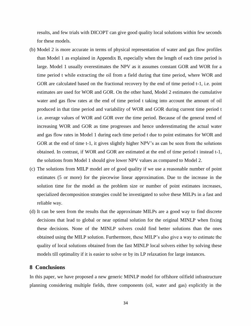
(b) Model 2 is more accurate in terms of physical representation of water and gas flow profiles

than Model 1 as explained in Appendix B, especially when the length of each time period is

large. Model 1 usually overestimates the NPV as it assumes constant GOR and WOR for a

time period t while extracting the oil from a field during that time period, where WOR and

GOR are calculated based on the fractional recovery by the end of time period t-1, i.e. point

estimates are used for WOR and GOR. On the other hand, Model 2 estimates the cumulative

water and gas flow rates at the end of time period t taking into account the amount of oil

produced in that time period and variability of WOR and GOR during current time period t

i.e. average values of WOR and GOR over the time period. Because of the general trend of

increasing WOR and GOR as time progresses and hence underestimating the actual water

and gas flow rates in Model 1 during each time period t due to point estimates for WOR and

GOR at the end of time t-1, it gives slightly higher NPV’s as can be seen from the solutions

obtained. In contrast, if WOR and GOR are estimated at the end of time period t instead t-1,

the solutions from Model 1 should give lower NPV values as compared to Model 2.

(c) The solutions from MILP model are of good quality if we use a reasonable number of point

estimates (5 or more) for the piecewise linear approximation. Due to the increase in the

solution time for the model as the problem size or number of point estimates increases,

specialized decomposition strategies could be investigated to solve these MILPs in a fast and

reliable way.

(d) It can be seen from the results that the approximate MILPs are a good way to find discrete

decisions that lead to global or near optimal solution for the original MINLP when fixing

these decisions. None of the MINLP solvers could find better solutions than the ones

obtained using the MILP solution. Furthermore, these MILP’s also give a way to estimate the

quality of local solutions obtained from the fast MINLP local solvers either by solving these

models till optimality if it is easier to solve or by its LP relaxation for large instances.

8 Conclusions

In this paper, we have proposed a new generic MINLP model for offshore oilfield infrastructure

planning considering multiple fields, three components (oil, water and gas) explicitly in the

35

formulation, facility expansions decisions and nonlinear reservoir profiles. The model can

determine the installation and expansion schedule of facilities and respective oil, liquid and gas

capacities, connection between the fields and FPSO’s, well drilling schedule and production rates

of oil, water and gas simultaneously in a multiperiod setting. The resulting model yields good

solutions to realistic instances when solving with DICOPT directly. Furthermore, the model can

be reformulated into an MILP using piecewise linearization and exact linearization techniques

with which the problem can be solved to global optimality. The proposed MINLP and MILP

formulations are further improved by using a binary reduction scheme resulting in the improved

local solutions and more than an order of magnitude reduction in the solution times. Realistic

instances involving 10 fields, 3 FPSO’s and 20 years planning horizon have been solved and

comparisons of the computational performance of the proposed MINLP and MILP formulations

are presented. Moreover, the models presented here are very generic and can either be used for

simplified cases (e.g. linear profiles for reservoir, fixed well schedule etc.) or extended to include

other complexities. There are various trade-offs involve in selecting a particular model for

oilfield problem. In case that we are concerned with the solution time, especially for the large

instances, it would be better to use DICOPT on Model 2R directly that gives good quality

solution very fast. If fast computing times are of no much concern one may want to use MILP

approximation model that can yield better solutions but at higher computational cost.

Furthermore, these MILP solutions also provide a way to access the quality of suboptimal

solutions from the MINLPs or finding better once using its solution for the original problem.

9 Acknowledgements

The authors acknowledge to ExxonMobil Upstream Research Company for the financial support

of this work.

References

Aronofsky JS, Williams AC. The use of linear programming and mathematical models in

underground oil production. Manage Sci. 1962; 8:394–407.

Aseeri, A., Gorman, P., Bagajewicz, M. J., Financial risk management in offshore oil

infrastructure planning and scheduling. Ind. Eng. Chem. Res. 2004, 43, 3063–3072.

36

Babusiaux, D., Favennec, J., Bauquis, P., Bret-Rouzaut, N., & Guirauden, D. 2004. Oil and gas

exploration and production—reserves, costs, contracts. Technip.

Behrenbruch, P. Offshore oilfield development planning. J. Pet. Technol. 1993, 45 (8), 735–743.

Bohannon J. A linear programming model for optimum development of multi-reservoir pipeline

systems. J Petrol Tech. 1970;22:1429–1436.

Carvalho, M., Pinto, J. M. A bilevel decomposition technique for the optimal planning of

offshore platforms. Brazilian J. Chem. Eng. 2006, 23, 67–82.

Carvalho, M., Pinto, J. M. An MILP model and solution technique for the planning of

infrastructure in offshore oilfields. J. Pet. Sci. Eng. 2006,51, 97–110.

Elgsæter, S. M., O. Slupphaug, Johansen T. A. A structured approach to optimizing offshore oil

and gas production with uncertain models. Comput. Chem. Eng. 2010, 34(2), 163-176.

Glover, F., Improved Linear Integer Programming Formulations of Nonlinear Integer Problems.

Management Science 1975, 22, (4), 455.

Goel, V., Grossmann, I. E. A stochastic programming approach to planning of offshore gas field

developments under uncertainty in reserves. Comput. Chem. Eng. 2004, 28 (8), 1409–1429.

Goel, V., Grossmann, I. E. A class of stochastic programs with decision dependent uncertainty.

Mathematical Programming, 2006, 108(2–3, Ser. B), 355–394.

Goel, V., Grossmann, I. E., El-Bakry, A. S., Mulkay, E. L. A novel branch and bound algorithm

for optimal development of gas fields under uncertainty in reserves. Comput. Chem. Eng. 2006,

30, 1076-1092.

Gupta, V., Grossmann, I. E. Solution strategies for multistage stochastic programming with

endogenous uncertainties. Comput. Chem. Eng. 2011, 35, 2235–2247.

Haugland, D., Hallefjord, Å., Asheim, H. Models for Petroleum Field Exploitation. Eur. J. Oper.

Res. 1988, 37, 58.

Iyer, R. R., Grossmann, I. E., Vasantharajan, S., Cullick, A. S. Optimal planning and scheduling

offshore oilfield infrastructure investment and operations. Ind. Eng. Chem. Res. 1998, 37, 1380–

1397.

Jonsbraten, T. W. Oil-field optimization under price uncertainty. Journal of the Operational

Research Society,1998, 49, 811.

37

Jonsbraten, T. W., Wets, R. J. B., Woodruff, D. L. A class of stochastic programs with decision

dependent random elements. Ann. Oper. Res. 1998, 82, 83–106.

Lee AS, Aronofsky JS. A linear programming model for scheduling crude oil production. J

Petrol Tech. 1958;10:51–54.

Lin, X., Floudas, C. A. A Novel Continuous-Time Modeling and Optimization Framework for

Well Platform Planning Problems. Optim. Eng. 2003, 4 (1-2), 65–95.

Ortiz-Gomez, A., Rico-Ramirez, V., & Hernandez-Castro, S. Mixed-integer multiperiod model

for the planning of oil-field production. Comput. Chem. Eng.,2002, 26(4–5), 703.

Sullivan J. A computer model for planning the development of an offshore gas field. J Petrol

Tech. 1982;34:1555–1564.

Tarhan, B., Grossmann, I.E., Goel, V. Stochastic programming approach for the planning of

offshore oil or gas field infrastructure under decision- dependent uncertainty. Ind. Eng. Chem.

Res. 2009, 48(6), 3078–3097.

Tarhan, B., Grossmann, I.E., Goel, V. Computational strategies for non-convex multistage

MINLP models with decision-dependent uncertainty and gradual uncertainty resolution. Ann.

Oper. Res., 2011, DOI: 10.1007/s10479-011-0855-x.

Tsarbopoulou, C. Optimization of oil facilities and oil production. M.Sc. Dissertation, University

College London, London, U.K., 2000.

Ulstein, N. L., Nygreen, B., Sagli, J. R. Tactical planning of offshore petroleum production. Eur.

J. Oper. Res. 2007, 176, 550–564.

van den Heever, S. A., Grossmann, I. E. An iterative aggregation/disaggregation approach for the

solution of a mixed integer nonlinear oilfield infrastructure planning model. Ind. Eng. Chem.

Res. 2000, 39, 1955–1971.

van den Heever, S. A., Grossmann, I. E., Vasantharajan, S.; Edwards, K. Integrating complex

economic objectives with the design and planning of offshore oilfield infrastructures. Comput.

Chem. Eng. 2000, 24, 1049–1055.

van den Heever, S. A., Grossmann, I. E. A Lagrangean Decomposition Heuristic for the Design

and Planning of Offshore Hydrocarbon Field Infrastructures with Complex Economic

Objectives. Ind. Eng. Chem. Res. 2001, 40, 2857–2875.

Li X., Armagan E., Tomasgard A., and Barton P. I. Stochastic pooling problem for natural gas

production network design and operation under uncertainty. AIChE J., 2010. In Press.

38

Nomenclature

Indices

t, τ time periods, { }

f field

fpso FPSO facility

Binary Variables

whether or not FPSO facility fpso is installed at the beginning of time period t

whether or not FPSO facility fpso is expanded at the beginning of time period t

whether or not a connection between field f and FPSO facility fpso is installed at

the beginning of time period t

whether or not a connection between field f and FPSO facility fpso is installed

Integer Variables

Number of wells drilled in field f at the beginning of time period t

Number of wells available in field f for production in time period t

Continuous Variables

NPV net present value

total revenues in time period t

total costs in time period t

total capital costs in time period t

total operating costs in time period t

total oil flow-rate in time period t

total water flow-rate in time period t

total gas flow-rate in time period t

oil production rate from field f in time period t

water production rate from field f in time period t

gas production rate from field f in time period t

cumulative oil produced from field f by the end of time period t

39

cumulative water produced from field f to FPSO facility fpso by the end of time

period t

cumulative gas produced from field f to FPSO facility fpso by the end of time

period t

fraction of oil recovered from field f by the end of time period t

oil flow rate per well from field f to FPSO facility fpso in time period t

field deliverability (maximum oil flow rate) per well for field f and FPSO facility

fpso combination in time period t

dummy variable for cumulative water produced from field f to FPSO facility fpso

by the end of time period t

dummy variable for cumulative gas produced from field f to FPSO facility fpso

by the end of time period t

total oil flow rate into FPSO facility fpso in time period t

total water flow rate into FPSO facility fpso in time period t

total gas flow rate into FPSO facility fpso in time period t

total oil flow rate from field f to FPSO facility fpso in time period t

total water flow rate from field f to FPSO facility fpso in time period t

total gas flow rate from field f to FPSO facility fpso in time period t

oil processing capacity of FPSO facility fpso in time period t

liquid (oil and water) capacity of FPSO facility fpso in time period t

gas capacity of FPSO facility fpso in time period t

oil installation capacity of FPSO facility fpso at the beginning of time period t

liquid installation capacity of FPSO facility fpso at the beginning of time period t

gas installation capacity of FPSO facility fpso at the beginning of time period t

oil expansion capacity of FPSO facility fpso at the beginning of time period t

liquid expansion capacity of FPSO facility fpso at the beginning of time period t

gas expansion capacity of FPSO facility fpso at the beginning of time period t

40

Parameters

fixed capital cost for installing FPSO facility fpso at the beginning of time period t

fixed cost for installing the connection between field f and FPSO facility fpso at

the

beginning of time period t

fixed cost for drilling a well in field f at the beginning of time period t

variable capital cost for installing or expanding the liquid (oil and water) capacity

of FPSO facility fpso at the beginning of time period t

variable capital cost for installing or expanding the gas capacity of FPSO facility

fpso at the beginning of time period t

operating cost for per unit of liquid (oil and water) produced in time period t

operating cost for per unit of gas produced in time period t

RECf total amount of recoverable oil from field f

Upper bound on the oil flow rate per well from field f to FPSO facility fpso

Upper bound on the installation or expansion of oil capacity of a FPSO facility

Upper bound on the installation or expansion of liquid capacity of a FPSO facility

Upper bound on the installation or expansion of gas capacity of a FPSO facility

Maximum number of wells that can be drilled in field f during planning horizon T

Maximum number of wells that can be drilled during each time period t

Maximum cumulative water that can be produced for a field-FPSO connection

Maximum cumulative gas that can be produced for a field-FPSO connection

l1 lead time for initial installation of a FPSO facility

l2 lead time for expansion of an earlier installed FPSO facility

µ Maximum fraction of the initial built FPSO capacities that can be expanded

αt price of oil in time period t

βt price of gas in time period t

dt discounting factor for time period t

δt number of days in time period t

a( ),b( ),c( ),d( ) coefficients for polynomials used for reservoir models

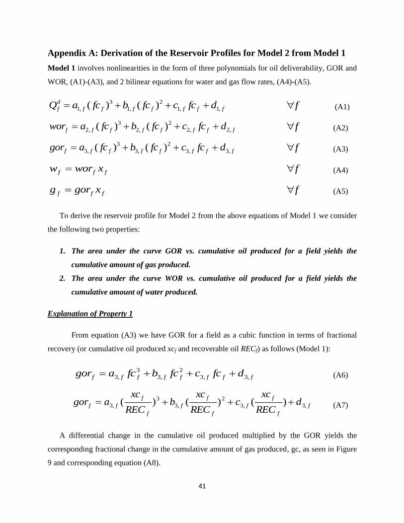
41

Appendix A: Derivation of the Reservoir Profiles for Model 2 from Model 1

Model 1 involves nonlinearities in the form of three polynomials for oil deliverability, GOR and

WOR, (A1)-(A3), and 2 bilinear equations for water and gas flow rates, (A4)-(A5).

fffffff

d

f dfccfcbfcaQ ,1,1

2

,1

3

,1 )()(

f

(A1)

ffffffff dfccfcbfcawor ,2,2

2

,2

3

,2 )()( f

(A2)

ffffffff dfccfcbfcagor ,3,3

2

,3

3

,3 )()( f (A3)

fff xworw

f (A4)

fff xgorg

f (A5)

To derive the reservoir profile for Model 2 from the above equations of Model 1 we consider

the following two properties:

1. The area under the curve GOR vs. cumulative oil produced for a field yields the

cumulative amount of gas produced.

2. The area under the curve WOR vs. cumulative oil produced for a field yields the

cumulative amount of water produced.

Explanation of Property 1

From equation (A3) we have GOR for a field as a cubic function in terms of fractional

recovery (or cumulative oil produced xcf and recoverable oil RECf) as follows (Model 1):

ffffffff dfccfcbfcagor ,3,3

2

,3

3

,3

(A6)

f

f

f

f

f

f

f

f

f

ff dREC

xcc

REC

xcb

REC

xcagor ,3,3

2

,3

3

,3 )()()(

(A7)

A differential change in the cumulative oil produced multiplied by the GOR yields the

corresponding fractional change in the cumulative amount of gas produced, gc, as seen in Figure

9 and corresponding equation (A8).

42

)(.)( fff xcdgorgcd

(A8)

We should note that Figure 9 corresponds to gor vs fc but it is easy to convert it to gor vs

xc given that the reservoir size (RECf) is known. Integrating in (A8) both sides from zero (i.e.

area under the curve between GOR and xc), yields,

ff xc

ff

gc

f xcdgorgcd00

)(.)(

(A9)

)(.)()()()(0

,3,3

2

,3

3

,3

0

f

xc

f

f

f

f

f

f

f

f

f

f

gc

f xcddREC

xcc

REC

xcb

REC

xcagcd

ff

(A10)

)()(2

)(3

)(4

,3

2

,3

2

3

,3

3

4

,3

ff

f

ff

f

ff

f

ff

f xcdREC

xcc

REC

xcb

REC

xcagc (A11)

)(.)(2

.)(

3

.)(

4

.,3

2,33,34,3

f

f

ff

f

fff

f

fff

f

fff

fREC

xcRECd

REC

xcRECc

REC

xcRECb

REC

xcRECagc

(A12)

)(.)(2

.)(

3

.)(

4

.,3

2,33,34,3

ffff

ff

f

ff

f

ff

f fcRECdfcRECc

fcRECb

fcRECa

gc

(A13)

0

0.2

0.4

0.6

0.8

1

1.2

0 0.2 0.4 0.6 0.8 1

GO

R (

kscf

/stb

)

fc

GOR gor(F1-FPSO1)

Figure 9: GOR profile for field (F1) and FPSO (FPSO 1) connection

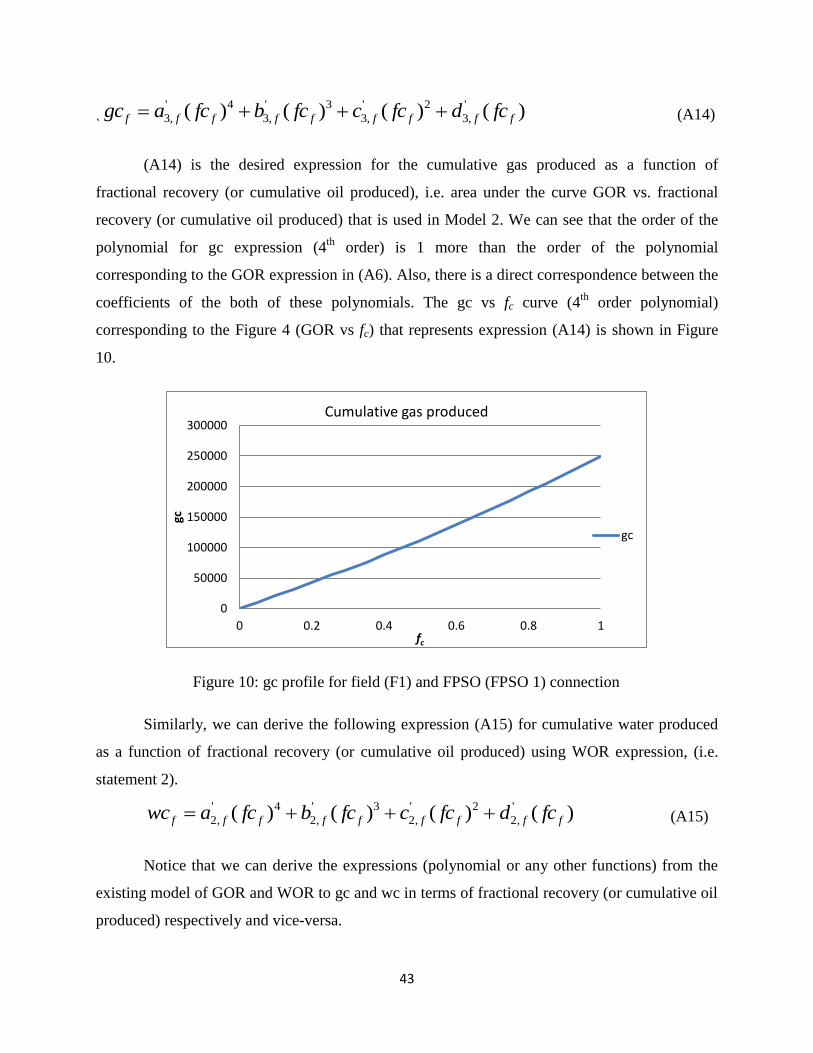
43

`)()()()( '

,3

2'

,3

3'

,3

4'

,3 fffffffff fcdfccfcbfcagc

(A14)

(A14) is the desired expression for the cumulative gas produced as a function of

fractional recovery (or cumulative oil produced), i.e. area under the curve GOR vs. fractional

recovery (or cumulative oil produced) that is used in Model 2. We can see that the order of the

polynomial for gc expression (4th

order) is 1 more than the order of the polynomial

corresponding to the GOR expression in (A6). Also, there is a direct correspondence between the

coefficients of the both of these polynomials. The gc vs fc curve (4th

order polynomial)

corresponding to the Figure 4 (GOR vs fc) that represents expression (A14) is shown in Figure

10.

Similarly, we can derive the following expression (A15) for cumulative water produced

as a function of fractional recovery (or cumulative oil produced) using WOR expression, (i.e.

statement 2).

)()()()( '

,2

2'

,2

3'

,2

4'

,2 fffffffff fcdfccfcbfcawc

(A15)

Notice that we can derive the expressions (polynomial or any other functions) from the

existing model of GOR and WOR to gc and wc in terms of fractional recovery (or cumulative oil

produced) respectively and vice-versa.

0

50000

100000

150000

200000

250000

300000

0 0.2 0.4 0.6 0.8 1

gc

fc

Cumulative gas produced

gc

Figure 10: gc profile for field (F1) and FPSO (FPSO 1) connection

44

Appendix B: Comparisons of the Models based on (gor, wor) and (gc, wc)

functions

1. Model 1 (GOR and WOR as a function of cumulative oil produced) requires the bilinear

equations (B1) and (B2) for water and gas flow rates while Model 2 does not need these

equations as these flowrates can be expressed as equations (B3) and (B4) given that we have

polynomials for gc and wc. Hence, Model 2 involving only univariate polynomials should

computationally perform better.

tftftf xgorg ,,, tf ,

(B1)

tftftf xworw ,,, tf , (B2)

ttftftf gcgcg /)( 1,,, tf , (B3)

ttftftf wcwcw /)( 1,,, tf , (B4)

2. The WOR and GOR functions in (A2) and (A3) introduce a large number of non-convexities

in Model 1 as compared to the gc and wc functions in (A14) and (A15) that are univariate

monotonically increasing functions. Hence, these functions will be better for approximating

them by piecewise linearization. As an example the GOR and corresponding gc functions for

a field are shown in Figure 11.

3. In Model 1 we assume that the WOR and GOR equations (B5) and (B6) used in time period t

are calculated in terms of the fractional oil recovery by the end of previous time period t-1,

0

0.2

0.4

0.6

0.8

1

1.2

1.4

0 0.5 1

GO

R (

kscf

/stb

)

fc

GOR

gor(F2-FPSO2)

gor(F2-FPSO3)

0

0.2

0.4

0.6

0.8

1

0 0.5 1

gc/R

EC*1

00

0

fc

gc

gc(F2-FPSO2)

gc(F2-FPSO3)

Figure 11: GOR and gc profiles for 1 field and 2 FPSO connections

45

i.e. uses point estimate values. Therefore, GOR and WOR essentially perform as constants in

current time period t, and the oil flowrate does not account for the variability in GOR and

WOR values during that time period.

ftfftfftfftf dfccfcbfcawor ,21,,2

2

1,,2

3

1,,2, )()( tf ,

(B5)

ftfftfftfftf dfccfcbfcagor ,31,,3

2

1,,3

3

1,,3, )()( tf ,

(B6)

tftftf xworw ,,, tf , (B7)

tftftf xgorg ,,, tf , (B8)

However, equations (B9) and (B10) for wc and gc explicitly predicts the cumulative amount

of water and gas produced, respectively, by the end of period t as a function of cumulative oil

produced by the end of period t, and hence also accounts for the variability of the GOR and

WOR values during current period t i.e. considers average values of WOR and GOR over the

time period t. Therefore, Model 2 is also better in terms of representing the physical reservoir

characteristics.

ftfftfftfftf dfccfcbfcawc ,2,,2

2

,,2

3

,,2, )()( tf , (B9)

ftfftfftfftf dfccfcbfcagc ,3,,3

2

,,3

3

,,3, )()( tf ,

(B10)

Notice that equations (B5) and (B6) for Model 1 could also be represented as a function of

fractional recovery by the end of time period t instead of time period t-1, however, the model

will still consider the WOR and GOR values based on the point estimate instead average values

over the time period t as used in Model 2.