Uncoupling of coupled flows in soil-a finite element method · PDF file · 2013-01-23ELEMENT METHOD DAICHAO SHENG* AND ... x3)=, the space coordinate vector, R is the space domain

INTERNATIONAL JOURNAL FOR NUMERICAL AND ANALYTICAL METHODS I N GEOMECHANICS, VOL. 19,537-553 (1995)

UNCOUPLING OF COUPLED FLOWS IN SOIL-A FINITE ELEMENT METHOD

DAICHAO SHENG* AND KENNET AXELSSON'

Department of Civil Engineering, Lulea University of Technology, 5-97187 Luled, Sweden

SUMMARY

Coupled flow of water, chemicals, heat and electrical potential in soil are of significance in a variety of circumstances. The problem is characterized by the coupling between different flows, i.e. a flow of one type driven by gradients of other types, and by the dual nature of certain flows, i.e. combined convection and conduction. Effective numerical solutions to the problem are challenged due to the coupling and the dual nature.

In this paper, we first present a general expression that can be used to represent various types of coupled flows in soil. A finite element method is then proposed to solve the generalized coupled flows of convection-conduction pattern. The unknown vector is first decomposed into two parts, a convective part forming a hyperbolic system and a conductive part forming a parabolic system. At each time step, the hyperbolic system is solved analytically to give an initial solution. To solve the multi-dimensional hyperbolic system, we assume that a common eigenspace exists for the coefficient matrices, so that the system can be uncoupled by transforming the unknown vector to the common eigenspace. The uncoupled system is solved by the method of characteristics. Using the solution of the hyperbolic system as the initial condition, we then solve the parabolic system by a Galerkin finite element method for space discretization and a finite difference scheme for time stepping.

The proposed technique can be used for solving multi-dimensional, transient, coupled or simultaneous flows of convection-conduction type. Application to a flow example shows that the technique indeed exhibits optimality in convergence and in stability.

INTRODUCTION

Coupled flows take place when a flow of one type is induced by gradients of other types, such as a hydraulic flow caused by an electrical gradient. In geotechnical engineering, we are already familiar with direct flows like water flow caused by hydraulic gradient, heat flow by temperature gradient, and chemical flow by concentration gradient. However, these direct flows often occur simultaneously and interact with one another. The constitutive relationships for the direct flows, such as the Darcy law for water flow, the Fourier law for heat conduction, the Fick law for chemical diffusion and the Ohm law for electrical current, are not sufficient to desoribe coupled flows. Recently Mitchell' has given a review of conduction phenomena in soils, with emphasis on coupled flows. Yeung and Mitchell' have developed the general formulation of coupled flows that are caused by hydraulic, electrical and chemical gradients.

The significance of coupled flows in geotechnical engineering has been assessed by Mitchell.' Some interesting applications in geotechnical engineering are given as follows.

*Senior Research Engineer 'Professor of Civil Engneering

CCC 0363-906 1/95/080537- 17 0 1995 by John Wiley & Sons, Ltd.

Received 12 November 1993 Revised 13 March 1995

538 D. SHENG AND K. AXELSSON

(1) Coupled heat and moisture flows in porous media. Moisture, both liquid and vapour phases, can move under pressure and temperature gradients in porous media like soil and concrete. Examples of related problems are thermal stability of buried power cable backfill, of heat storage and of nuclear waste disposal,'.3 fire response of concrete structure^,^ and freezing of fined-grained soils.5

( 2 ) Coupled or simultaneous flows of water, chemical and heat. Chemical components flow in the ground under gradients of concentration, hydraulic head and temperature. Examples refer to contaminant transport in groundwater,6. diffusive chemical flow through a landfill linear,'q9 gas diffusion in soils.'O

(3) Coupled hydraulic, electrical and chemical flows. Examples of application include electro- osmotic consolidation,' chemico-osmotic cons~lidation,~* '' electro-kinetics in waste con- tainment and cleanup of contaminated sites,', '' electro-osmosis for stabilization of a foun- dation on a soft clay,' influence of coupled flows on slope ~tability.'. '~

According to Yeung and Mitchell,' coupled flows by conduction can be expressed by n

j = 1

where JD denotes the conductive flow of type i, X j the gradient of type j , K i j the phenomenological coefficient relating the flow of type i to the gradient of type j . If the flow and the gradient are of the same type, i.e. i = j , we return to the known coefficients like the hydraulic conductivity, the thermal conductivity, the diffusivity and the electrical conductivity. The coupling coefficients Kij when i # j are usually assumed to follow the Onsager reciprocal relations, i.e. K i j = K j i . Particular values of such coefficients have been discussed by Mitchell' and by Yeung and Mitchell.'

Besides the coupling of conduction between different flow, another important feature of flows in soil is the dual nature of certain flows due to combination of convection and conduction. The total flux of a flow such as a heat flow and a chemical flow is

Ji = JD + J y + uiJw ( 2 )

where J i is the total flow of type i, JF the convective flow due to the fluid velocity, Lai an extensive quantity such as the enthalpy and the concentration, and J , the fluid velocity. When the convection parts J y are significant compared to the conduction parts, the conventional numerical solution techniques such as the central finite difference methods and the standard Galerkin finite element method are challenged in stability, convergence and accuracy.

Numerical solution to coupled flows excluding the convection term has been discussed by e.g. Lewis and Garner,14 Lewis and H u m p h e s ~ n . ' ~ More recently, attention has been paid to numerical solutions to convective-conductive transport problems, and indeed effective solution techniques have been developed. Outstanding examples of such techniques include the Petrov-Galerkin methods and the characteristic-Galerkin methods. By a Petrov-Galerkin method, the weighting functions differ from the shape functions.16-" A typical example of such weighting methods is the so-called streamline upwind weighting. Although the Petrov-Galerkin methods generally give significant improvement on accuracy and stability over the standard Galerkin method, they are characterized by some artificial diffusion and by the restriction on the values of time step.

Another family of numerical methods used to solve convective-conductive equations is the so-called characteristic-Galerkin methods.'' -" B y a characteristic-Galerkin method, the finite element solutions are searched along the characteristics. An example of such methods is the

UNCOUPLING OF COUPLED FLOWS IN SOIL 539

Eulerian-Lagrangian finite element method proposed by Neuman,20s21 by which the unknown is decomposed into a convective part and a diffusive part, being solved respectively by an adaptive method of characteristics and a Galerkin finite element method. Sheng et ~ 1 . ’ ~ successfully applied this method to solve convective-conductive heat transfer with phase change. In this paper, a similar technique is applied to solve the multi-dimensional coupled flow problem.

GENERALIZED GOVERNING EQUATIONS

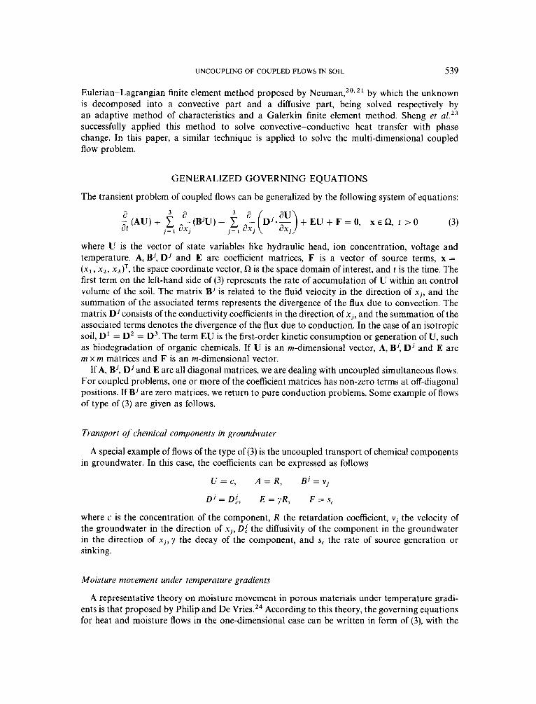
The transient problem of coupled flows can be generalized by the following system of equations:

where U is the vector of state variables like hydraulic head, ion concentration, voltage and temperature. A, Bj, Dj and E are coefficient matrices, F is a vector of source terms, x = (xl, x2, x3)=, the space coordinate vector, R is the space domain of interest, and t is the time. The first term on the left-hand side of (3) represents the rate of accumulation of U within an control volume of the soil. The matrix B’ is related to the fluid velocity in the direction of x j , and the summation of the associated terms represents the divergence of the flux due to convection. The matrix D’consists of the conductivity coefficients in the direction of xj, and the summation of the associated terms denotes the divergence of the flux due to conduction. In the case of an isotropic soil, D’ = D2 = D3. The term EU is the first-order kinetic consumption or generation of U, such as biodegradation of organic chemicals. If U is an m-dimensional vector, A, B’, D’ and E are m x m matrices and F is an rn-dimensional vector.

If A, B’, Dj and E are all diagonal matrices, we are dealing with uncoupled simultaneous flows. For coupled problems, one or more of the coefficient matrices has non-zero terms at off-diagonal positions. If B’ are zero matrices, we return to pure conduction problems. Some example of flows of type of (3) are given as follows.

Transport of chemical components in groundwater

A special example of flows of the type of (3) is the uncoupled transport of chemical components in groundwater. In this case, the coefficients can be expressed as follows

U = C, A = R, B ’ = ~j

D j = Df, E = y R , F = s ,

where c is the concentration of the component, R the retardation coefficient, vj the velocity of the groundwater in the direction of x j , D! the diffusivity of the component in the groundwater in the direction of x i , ? the decay of the component, and s, the rate of source generation or sin king.

Moisture movement under temperature gradients

A representative theory on moisture movement in porous materials under temperature gradients is that proposed by Philip and De Vr ie~ . ’~ According to this theory, the governing equations for heat and moisture flows in the one-dimensional case can be written in form of (3), with the


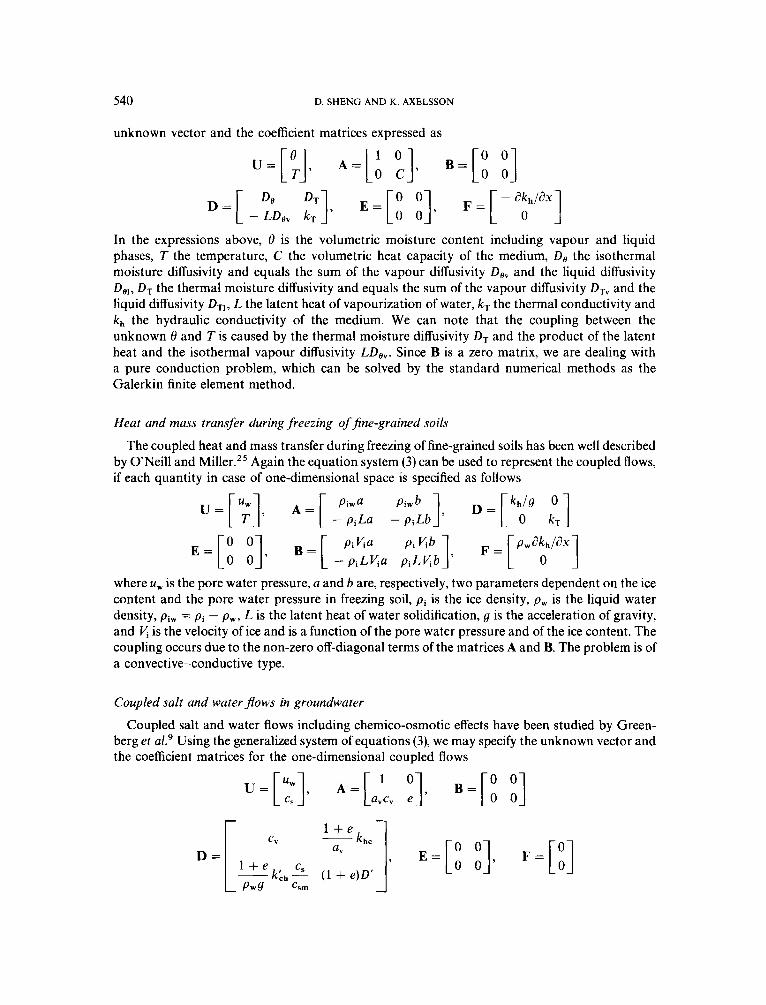
unknown vector and the coefficient matrices expressed as

u=[;], A=[; "c3. B = [ o 0 0 03

In the expressions above, 8 is the volumetric moisture content including vapour and liquid phases, T the temperature, C the volumetric heat capacity of the medium, De the isothermal moisture diffusivity and equals the sum of the vapour diffusivity DBv and the liquid diffusivity Do,, DT the thermal moisture diffusivity and equals the sum of the vapour diffusivity D T v and the liquid diffusivity DTI, L the latent heat of vapourization of water, kT the thermal conductivity and kh the hydraulic conductivity of the medium. We can note that the coupling between the unknown 8 and T is caused by the thermal moisture diffusivity DT and the product of the latent heat and the isothermal vapour diffusivity LDB,. Since B is a zero matrix, we are dealing with a pure conduction problem, which can be solved by the standard numerical methods as the Galerkin finite element method.

Heat and mass transfer during freezing of fine-grained soils

The coupled heat and mass transfer during freezing of fine-grained soils has been well described by ONeill and Miller.25 Again the equation system (3) can be used to represent the coupled flows, if each quantity in case of one-dimensional space is specified as follows

where u, is the pore water pressure, a and b are, respectively, two parameters dependent on the ice content and the pore water pressure in freezing soil, pi is the ice density, pw is the liquid water density, pi, = pi - p,, L is the latent heat of water solidification, g is the acceleration of gravity, and 6 is the velocity of ice and is a function of the pore water pressure and of the ice content. The coupling occurs due to the non-zero off-diagonal terms of the matrices A and B. The problem is of a convective-conductive type.

Coupled salt and water ffows in groundwater

Coupled salt and water flows including chemico-osmotic effects have been studied by Green- berg et aL9 Using the generalized system of equations (3), we may specify the unknown vector and the coefficient matrices for the one-dimensional coupled flows

r

UNCOUPLING OF COUPLED FLOWS IN SOIL 54 1

where c, is the salt concentration in groundwater, a, the coefficient of compressibility of the soil, e the void ratio, c, the coefficient of consolidation, khc and kbh the coupling coefficients, c,, the possible maximum value of c,, D’ the effective diffusion constant, and g the acceleration of gravity.

Consolidation of soils including electro-osmosis effects

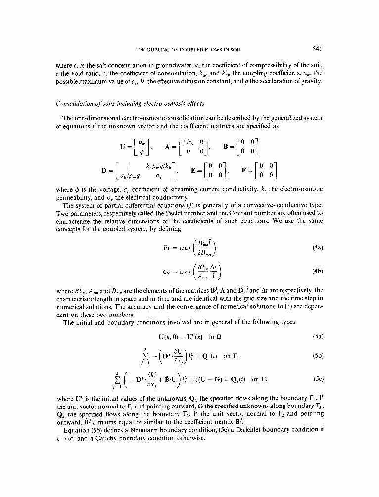
The one-dimensional electro-osmotic consolidation can be described by the generalized system of equations if the unknown vector and the coefficient matrices are specified as

.=[:I, A=[’:’ :], . = L o 0 0 0]

D = [ k e p w g ’ k h ] , .=[ 0 0 1, F = [ 0 0 ] fJh/Pwg fJe 0 0 0 0

where 4 is the voltage, gh coefficient of streaming current conductivity, k , the electro-osmotic permeability, and oe the electrical conductivity.

The system of partial differential equations (3) is generally of a convective-conductive type. Two parameters, respectively called the Peclet number and the Courant number are often used to characterize the relative dimensions of the coefficients of such equations. We use the same concepts for the coupled system, by defining

B’,,, At c o = max ( A,n 7)

where B’,,, A,, and D,, are the elements of the matrices Bj, A and D, rand At are respectively, the characteristic length in space and in time and are identical with the grid size and the time step in numerical solutions. The accuracy and the convergence of numerical solutions to (3) are dependent on these two numbers.

The initial and boundary conditions involved are in general of the following types

lj’ + E(U - G ) = Q2(t) on r, j = 1

where Uo is the initial values of the unknowns, Q1 the specified flows along the boundary r,, I’ the unit vector normal to r, and pointing outward, G the specified unknowns along boundary r,, Q2 the specified flows along the boundary r2, l2 the unit vector normal to r2 and pointing outward, B’ a matrix equal or similar to the coefficient matrix BJ.

Equation (5b) defines a Neumann boundary condition, (5c) a Dirichlet boundary condition if E -+ co and a Cauchy boundary condition otherwise.


DECOMPOSITION AND APPROXIMATION

First, let us rewrite the system of equations (3) in Lagrangian form

where

denotes the material derivative. Let a part of the unknown, say U, satisfy the following initial value problem

U(x, 0) = U(x, 0) = U"x) (8b)

The set of equations (8) represents a convection problem, which can be solved by the method of characteristics.

Subtracting @a) from (6) yields the following diffusion problem:

The initial condition for the diffusion problem becomes

U(x, 0) - U(x, 0) = 0 (9b)

The boundary conditions are described by (5b) and (5c). The diffusion problem defined by (9) and (5b) and (54 can be solved by the standard Galerkin finite element method. By such a method, the unknowns are approximated by

m

U z 1 Ni(x)Ui(t) = NU i = 1

where m is the number of nodes after space discretization; Ni the NiI, Ni shape functions, I a n x n identity matrix; Ui the values of U at node i, a n-dimensional vector; N the n x (n x m) matrix, consisting of Ni; U the (n x m)-dimensional vector, consisting of Ui.

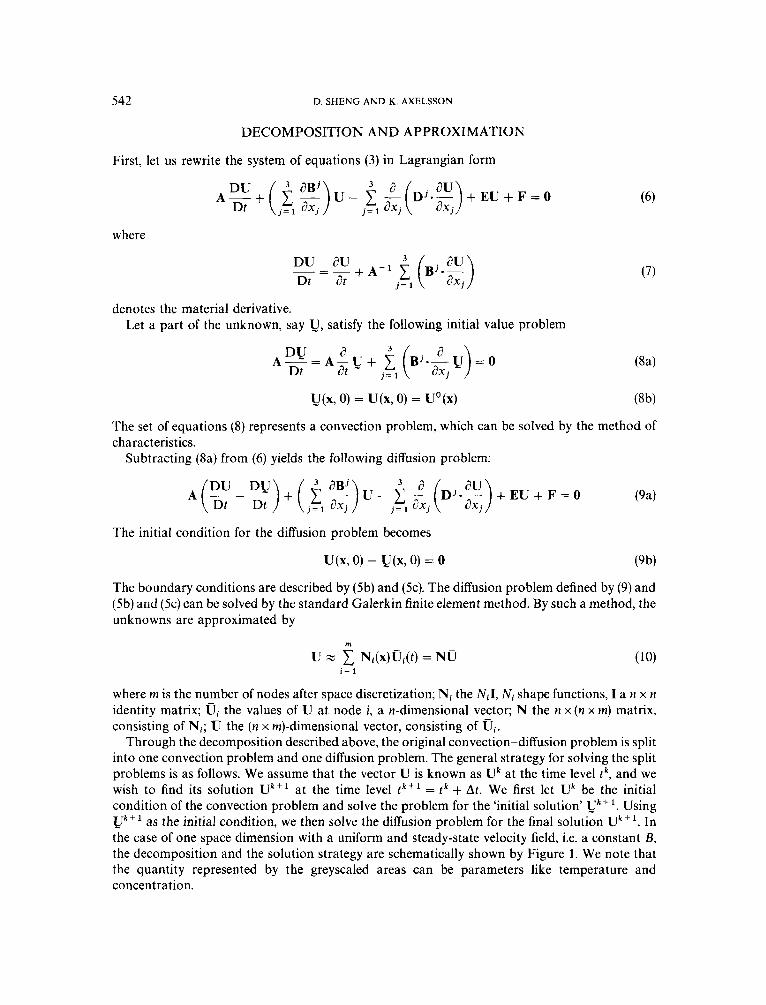
Through the decomposition described above, the original convection-diffusion problem is split into one convection problem and one diffusion problem. The general strategy for solving the split problems is as follows. We assume that the vector U is known as Uk at the time level tk , and we wish to find its solution Uk+' at the time level t k + ' = t k + At. We first let Uk be the initial condition of the convection problem and solve the problem for the 'initial solution' Uk+l. Using Uk+' - as the initial condition, we then solve the diffusion problem for the final solution Uk+'. In the case of one space dimension with a uniform and steady-state velocity field, i.e. a constant B, the decomposition and the solution strategy are schematically shown by Figure 1. We note that the quantity represented by the greyscaled areas can be parameters like temperature and concentration.


Figure 1. Schematic view of the decomposition of a convective-conductive transport

INITIAL SOLUTION BY CONVECTION

The matrix A is associated with the capacitance of the unknown U and is positive definite and invertible. In the case of a linear problem, the elements of the matrices A and B’ are constants or functions of x. In the case of a nonlinear problem, A or B’ may be functions of U and t. Since at each time step the unknown U is approximated by (lo), A and B’ can still be treated as only functions of x even for nonlinear cases. Therefore, the matrix products of A - ‘B’ ( j = 1,2,3) exist and the values of their elements can be determined a t each time step.

The hyperbolic system (8) can be uncoupled if the matrices A - ‘B’ ( j = 1,2,3) are all diagonalizable and share the same eigenvector matrix. The existence of a common eigenspace for three matrices requires one of the following conditions:

I. the three matrices are diagonalizable and commute with one another, or 11. the three matrices are all symmetric.

In general, the first requirement is satisfied for coupled flows of interest. In certain cases such as in the Philip and De Vries’ model of moisture and heat flow the second requirement is also satisfied. The physical implication of these requirements has to be discussed when we are dealing with particular flow and at this moment we reasonably assume that the system (8) can be uncoupled. Let us denote the common eigenvector matrix of A-’Bj ( j = 1,2 ,3) by P. We can then use P to introduce a new unknown vector W by the transformation

Substitution of (1 1) into (8a) gives


Multiplying by P-'A-' from the left of each term of (12) yields

where A = P- '(A-'B')P, the diagonal matrix with the eigenvalues of A-'BJ on its diagonal. The system of equations above consists of n uncoupled hyperbolic equations that can be solved independently. The solutions of W are constant along the characteristic curves defined by

- dX dt - _

dx: dx i dx: dt dt dt

dx: dx; dx:

- - _ _

- - - dt dt dt . . . . . . . . .

dx; dx; dx:

= A

- 1 1 1 1

where Ai is the ith eigenvalue of A-'BJ, X denote the characteristic curves of W, and xjldt defines the slope of the characteristics X i of U: in the direction of xj. Substitution of (1 1) into the initial condition (8b) gives the constant solutions of W along the characteristics X

W(X, t) = WO(X) = P-'UO(x) (15)

Along the characteristics defined by (14), the unknowns u are obviously constant too. The constant solutions are given by

U(X, t) = PW(X, t) = PP-'UO(x) = U"x) (16)

The solution technique described above can be applied node by node step by step. At any time level tk, the nodal values of U, known as Uk, can be treated as the initial condition of the convection problem. If the approximation defined by (10) is used, the initial condition for the convection is

n

U(X, tk) = U(X, t k ) = 1 Ni(x)Ui(tk) i = l

where Ui( tk ) is the values of U at the node i at the time level tk. If a fictitious particle that moves along a characteristic curve is exactly located at a nodal point at tk+', we can backwards track the particle to its original positions at tk

..

where X k is the positions of the nodal point x on the characteristic curves at tk. The system of equations above shows that the fictitious particle carries information from two different positions


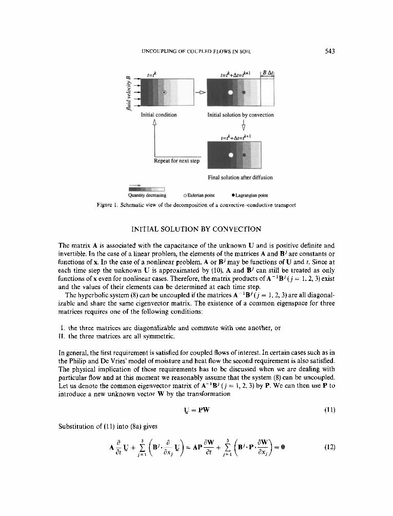
Figure 2. Characteristic lines and backward tracking for a two-flow system in one-dimensional space

for different unknowns if A1 # Az. These two positions X : and X$ are demonstrated in Figure 2. The values of !J at the nodal point at t k + ' can be determined by

m

Uk" - = u(X, t k + ' ) = V(Xk, t k ) = U(Xk, t k ) = C Ni(Xk)Ui(tk) (19) i = 1

In the case where no steep gradient in the unknowns is encountered, equations (18) and (19) give the initial solution Qk+ of the convection. Otherwise, continuous forward tracking of the steep gradients is needed.'l In this paper, we do not consider steep gradients. The solution of the convection given by (18) and (19) will be used as the initial condition for the diffusion problem, which will be solved numerically for the final solution Uk+'.

FINAL SOLUTION AFTER DIFFUSION

The diffusion problem defined by (9) and (5b) and (5c) can be solved by the standard Galerkin method. Using the approximation (10) and applying the Galerkin weighting procedure to (9a) lead to the following system of ordinary differential equations

where

M = NTANdx I,


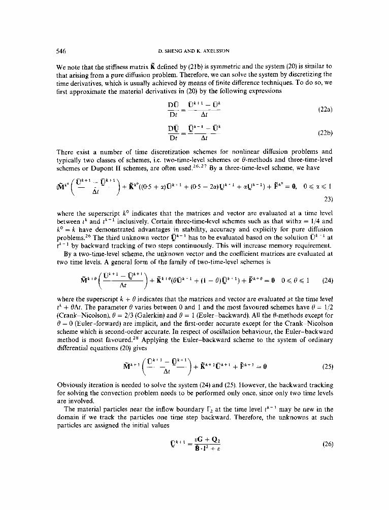
We note that the stiffness matrix g defined by (21b) is symmetric and the system (20) is similar to that arising from a pure diffusion problem. Therefore, we can solve the system by discretizing the time derivatives, which is usually achieved by means of finite difference techniques. To do so, we first approximate the material derivatives in (20) by the following expressions

There exist a number of time discretization schemes for nonlinear diffusion problems and typically two classes of schemes, i.e. two-time-level schemes or &methods and three-time-level schemes or Dupont I1 schemes, are often ~ s e d . ~ ~ , ~ ' By a three-time-level scheme, we have

where the superscript ko indicates that the matrices and vector are evaluated at a time level between tk and t k + ' inclusively. Certain three-time-level schemes such as that withcr = 1/4 and ko = k have demonstrated advantages in stability, accuracy and explicity for pure diffusion problems.26 The third unknown vector gk-' has to be evaluated based on the solution Uk- ' at t k - ' by backward tracking of two steps continuously. This will increase memory requirement.

By a two-time-level scheme, the unknown vector and the coefficient matrices are evaluated at two time levels. A general form of the family of two-time-level schemes is

where the superscript k + % indicates that the matrices and vector are evaluated at the time level t k + BAt. The parameter 8 varies between 0 and 1 and the most favoured schemes have 8 = 1/2 (Crank-Nicolson), 0 = 2/3 (Galerkin) and 6 = 1 (Euler-backward). All the &methods except for B = 0 (Euler-forward) are implicit, and the first-order accurate except for the Crank-Nicolson scheme which is second-order accurate. In respect of oscillation behaviour, the Euler-backward method is most favoured.28 Applying the Euler-backward scheme to the system of ordinary differential equations (20) gives

u k + 1

M k + I ( uk+'it - ) + g k + l f j k + l + @ k + l = O

Obviously iteration is needed to solve the system (24) and (25). However, the backward tracking for solving the convection problem needs to be performed only once, since only two time levels are involved.

The material particles near the inflow boundary r, at the time level tk+ ' may be new in the domain if we track the particles one time step backward. Therefore, the unknowns at such particles are assigned the initial values

547 UNCOUPLING OF COUPLED FLOWS IN SOIL

The same expression is valid for computing gk- near the inflow boundary, if the three-time-level scheme (23) is applied.

NUMERICAL EXAMPLE

So far, the problem has been discussed in general terms, i.e. for multi-flow systems in three- dimensional space for any type of elements with general shape functions. Computer implementation of a general solution to general coupled flows requires considerable programming work and right now we are not ready to present some results. However, it if possible to apply the solution technique to simple cases like a two-flow system in one-dimensional space, using linear elements and an explicit time-stepping scheme. The one-dimensional coupled heat and water flow in a freezing soil column can be used as such an example.

As is now understood, freezing of a moist soil is essentially a process of coupled heat and mass transfer. When a saturated fine-grained soil is subjected to a subfreezing temperature at e.g. its surface, part of the water in the soil pores close to the surface will solidify into ice, i t . pore ice particles, while close to the soil particles and more tightly bound to them films of unfrozen water remain. According to thermodynamics, these films of adsorbed water have a lower free energy at a lower negative temperature. Therefore, a potential gradient can develop along the temperature gradient. Water can be sucked from the warm portion to replace the amount of water lost due to freezing and to feed the accumulation of pore ice. As the temperature continues to decrease, the pore ice particles grow and the pressure is balanced by the pore pressure, the ice particles can finally contact each other and form an pure ice lens, oriented perpendicular to the direction of the heat and water flow. This ice lens, connected to the pore ice particles below in a warmer zone, will keep growing until a new ice lens forms at somewhere a warmer position. The soil will heave at approximately the same rate as the growth rate of ice lenses. The details about coupled heat and water flow, ice lens formation and frost heave in a freezing soil may refer to References 25 and 29.

There exists a number of models about the freezing process of a fine-grained soil. The frost heave model by ONeill and Miller 2 5 has been considered as the most complete and realistic one developed to date. However, the appearance of both the first and the second-order space derivatives in the governing equations has caused difficulties to solve the model effectively. O’Neill and Millerz5 tried to use a standard Galerkin method and they found that the numerical solutions became unstable during the terminal stage of heave, even cautious choice of the time step.

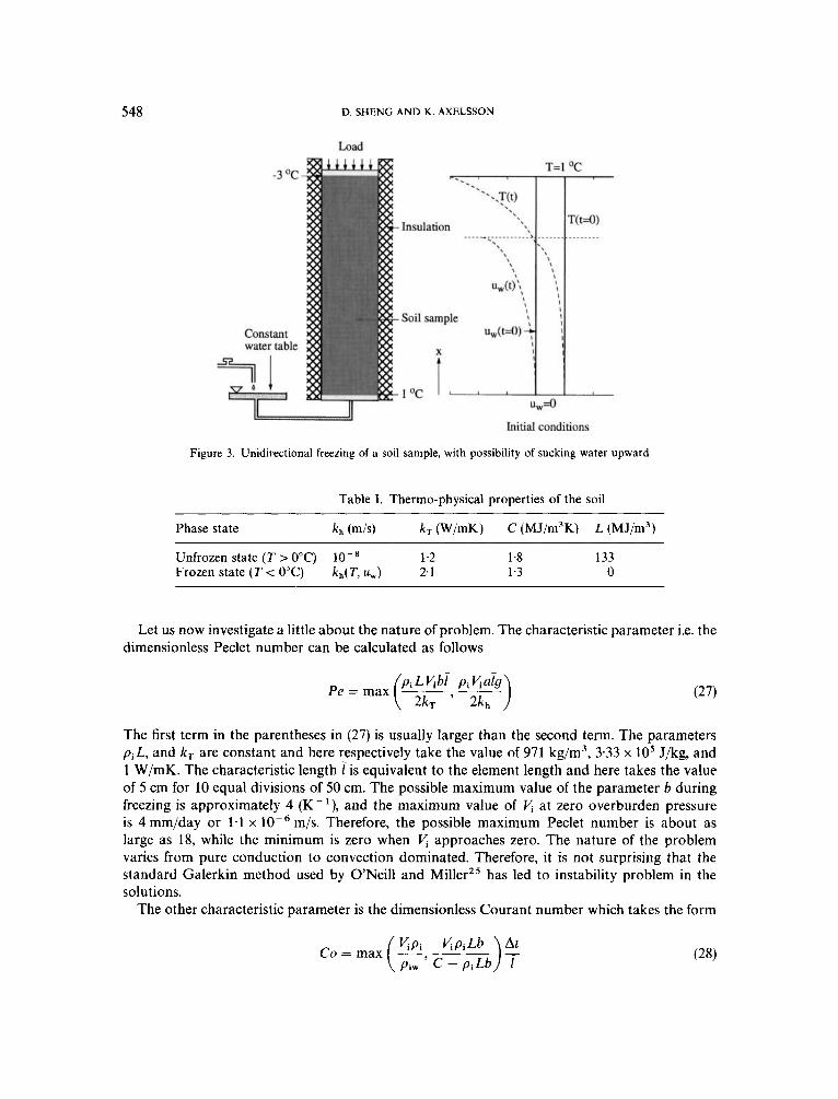
The problem can be illustrated by Figure 3. A soil sample of 50 cm in length is assumed to be insulated so that the lateral heat flow is negligible. The initial temperature in the sample is 1°C. At time zero the temperature at the top of the sample is dropped - 3°C while the temperature at the bottom remains 1°C. The bottom of the sample is connected to a constant water table so that water can be sucked upward during freezing. The sample is loaded at the top. The material properties of the samples is listed in Table I.

The main unknowns in the governing equations are the temperature and the pore water pressure. The ice content, the parameters a and b, the ice velocity, the vertical displacement or the heave, the ice pressure and the effective pore pressure or the neutral stress are intermediate unknowns which have to be evaluated based on the solutions of the main unknowns at each time step. The details about how to evaluate these intermediate unknowns may refer to References 25 and 29.


Figure 3. Unidirectional freezing of a soil sample, with possibility of sucking water upward

Table I. Thermo-physical properties of the soil

Phase state kh (m/s) kT (W/mK) C (MJ/m3K) L (MJ/m3)

Unfrozen state ( T > OOC) lo-* 1.2 1.8 133 Frozen state (T < 0°C) kh(T, u,) 2.1 1.3 0

Let us now investigate a little about the nature of problem. The characteristic parameter i.e. the dimensionless Peclet number can be calculated as follows

Pe = max (-, piLGbf piKaig -) 2kT 2kh

The first term in the parentheses in (27) is usually larger than the second term. The parameters piL, and kT are constant and here respectively take the value of 971 kg/m3, 3.33 x lo5 J/kg, and 1 W/mK. The characteristic length i is equivalent to the element length and here takes the value of 5 cm for 10 equal divisions of 50 cm. The possible maximum value of the parameter b during freezing is approximately 4 (IC'), and the maximum value of at zero overburden pressure is 4 mm/day or 1.1 x m/s. Therefore, the possible maximum Peclet number is about as large as 18, while the minimum is zero when approaches zero. The nature of the problem varies from pure conduction to convection dominated. Therefore, it is not surprising that the standard Galerkin method used by O'Neill and Millerz5 has led to instability problem in the solutions.

The other characteristic parameter is the dimensionless Courant number which takes the form


Courant Number

1 10 100 loo0 loo00 Time step (seconds) - characteristic-Galerkin method standard Galerkin method

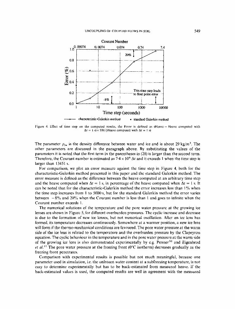
Figure 4. Effect of time step on the computed results, the Error is defined as (Heave - Heave computed with At = 1 s) x lOO/(Heave computed with At = 1 s)

The parameter piw is the density difference between water and ice and is about 29 kg/m3. The other parameters are discussed in the paragraph above. By substituting the values of the parameters it is noted that the first term in the parentheses in (28) is larger than the second term. Therefore, the Courant number is estimated as 7.4 x lo4 At and it exceeds 1 when the time step is larger than 13451 s.

For comparison, we plot an error measure against the time step in Figure 4, both for the characteristic-Galerkin method presented in this paper and the standard Galerkin method. The error measure is defined as the difference between the heave computed at an arbitrary time step and the heave computed when At = 1 s, in percentage of the heave computed when At = 1 s. It can be noted that for the characteristic-Galerkin method the error increases less than 1 % when the time step increases from 1 to 5000 s, but for the standard Galerkin method the error varies between -8% and 20% when the Courant number is less than 1 and goes to infinite when the Courant number exceeds 1.

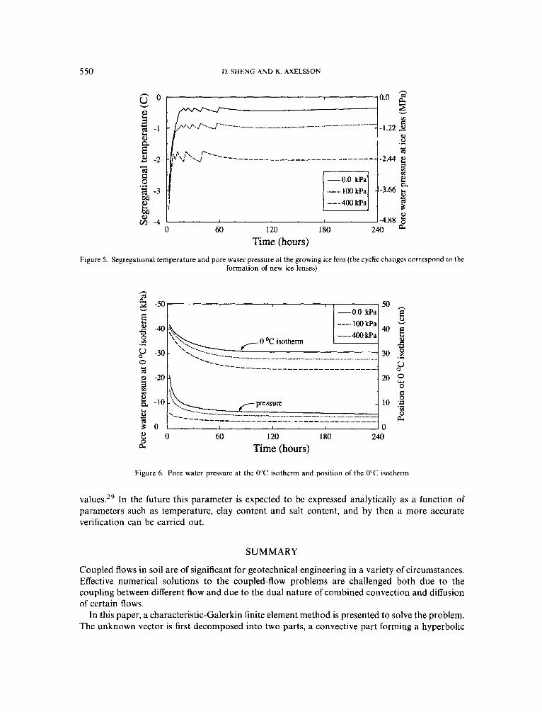
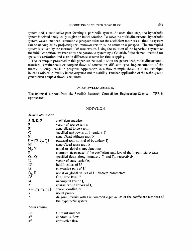
The numerical solutions of the temperature and the pore water pressure at the growing ice lenses are shown in Figure 5, for different overburden pressures. The cyclic increase and decrease is due to the formation of new ice lenses, but not numerical oscillation. After an ice lens has formed, its temperature decreases continuously. Somewhere at a warmer position, a new ice lens will form if the thermo-mechanical conditions are favoured. The pore water pressure at the warm side of the ice lens is related to the temperature and the overburden pressure by the Clapeyron equation. The cyclic behaviour in the temperature and in the pore water pressure at the warm side of the growing ice lens is also demonstrated experimentally by e.g. Penner3' and Eigenbrod et aL3' The pore water pressure at the freezing front (0°C isotherm) decreases gradually as the freezing front penetrates.

Comparison with experimental results is possible but not much meaningful, because one parameter used in simulation, i.e. the unfrozen water content at a subfreezing temperature, is not easy to determine experimentally but has to be back-estimated from measured heave. If the back-estimated values is used, the computed results are well in agreement with the measured

5 50 D. SHENG AND K. AXELSSON

0.0 G O -

2 3 - - -1.22 g -1

3 -2 - /,J'\p,J----- ----________________--------- -2.44

W

- 0 a E

I I

3

---400kPa

-4.88 240

co EI 0 .d Y co -3

$ - 4 L

0 60 120 180 Time (hours)

Figure 5. Segregational temperature and pore water pressure at the growing ice lens (the cyclicchanges correspond to the formation of new ice lenses)

Figure 6. Pore water pressure at the 0°C isotherm and position of the 0°C isotherm

values.29 In the future this parameter is expected to be expressed analytically as a function of parameters such as temperature, clay content and salt content, and by then a more accurate verification can be carried out.

SUMMARY

Coupled flows in soil are of significant for geotechnical engineering in a variety of circumstances. Effective numerical solutions to the coupled-flow problems are challenged both due to the coupling between different flow and due to the dual nature of combined convection and diffusion of certain flows.

In this paper, a characteristic-Galerkin finite element method is presented to solve the problem. The unknown vector is first decomposed into two parts, a convective part forming a hyperbolic


system and a conductive part forming a parabolic system. At each time step, the hyperbolic system is solved analytically to give an initial solution. To solve the multi-dimensional hyperbolic system, we assume that a common eigenspace exists for the coefficient matrices, so that the system can be uncoupled by projecting the unknown vector to the common eigenspace. The uncoupled system is solved by the method of characteristics. Using the solution of the hyperbolic system as the initial condition, we then solve the parabolic system by a Galerkin finite element method for space discretization and a finite difference scheme for time stepping.

The techniques presented in this paper can be used to solve the generalized, multi-dimensional, transient, simultaneous or coupled flows of convection-diffusion type. Implementation of the theory to computers is in progress. Application to a flow example shows that the technique indeed exhibits optimality in convergence and in stability. Further application of the technique to generalized coupled flows is required.

ACKNOWLEDGEMENTS

The financial support from the Swedish Research Council for Engineering Science - TFR is appreciated.

NOTATION

Matrix and vector

A, B, D, E F P G ii

N j , N P Q 1 , Qz U U0 I! ui, u uk

Latin notation

c o JD J C

coefficient matrices vector of source terms generalized force vector specified unknowns at boundary r, generalized stiffness matrix outward unit normal of boundary rj generalized mass matrix nodal or global shape functions common eigenspace of the coefficient matrices of the hyperbolic system specified flows along boundary r, and r,, respectively vector of state variables initial values of U convective part of U nodal or global values of U, discrete parameters D at time level tk uncoupled vector &J characteristic curves of &J space coordinates nodal points diagonal matrix with the common eigenvalues of the coefficient matrices of the hyperbolic system

Courant number conductive flow convective flow


K Pe X t At

Greek letters

n l-1, r2 A

phenomenological coefficient Peclet number gradient of e.g. hydraulic head, chemical concentration, temperature time time step

domain of interest boundaries of 0 eigenvalue

REFERENCES

1. J. K. Mitchell, ‘Conduction phenomena-from the theory to geotechnical practice: 31st Rankine Lecture’, Giotech-

2. A. T. Yeung and J. K. Mitchell, ‘Coupled fluid, electrical and chemical flows in soil’, Gkotechnique, 43(1), 121-134

3. H. S. Radhakrishna, K-C. Lau and A. M. Crawford, ‘Coupled heat and mositure through soils’, ASCE J . Geotech.

4. C. L. D. Huang and G. N. Ahmed, ‘Computational solution for heat and mass transfer in concrete slabs under fire’, in

5. R. D. Miller, ‘Freezing phenomena in soils’, in D. Hillel, (ed.), Application o f so i l Physics Academic Press, New York,

6. J. Bear and Y. Bachmat, Introduction to Modeling of Transport Phenomena in Porous Media, Kluwer Academic

7. H. E. Kobus and W. Kinzebach (eds.), Contaminant Transport in Groundwater, A. A. Balkema, Rotterdam, The

8. R. M. Quigely et al., ‘Hydraulic conductivity of contaminated natural clay directly below a domestic landfill, Can.

9. J. A. Greenberg, J. K. Mitchell and P. A. Witherspoon, ‘Coupled salt and water flows in groundwater basin’, J .

nique, 41(3), 299-340 (1991).

( 1993).

Eng., 110, 1766--1784 (1984).

R. W. Lewis and K. Morgan (eds), Num. Meth. in Thermal Problems, Pineridge Press, Swansea, U.K., 1989.

1982, pp. 254-299.

Publishers, The Netherlands, 1990.

Netherlands, 1989.

Geotech. J . , 20(2), 377-383 (1987).

Geophys. Res. 78, 6341-6353 (1973). 10. W. A. Jury, W. R. Gardner and W. H. Gardner, Soil Physics, 5th edn, Wiley, New York, 1991. 11. J. K. Mitchell, J. A. Greenberg and P. A. Witherspoon, ‘Chemico-osmotic effects in fine-grained soils’, ASCE J . Soil

12. D. Cabrera-Guzman, J. T. Swartzbaugh and A. W. Weisman, ‘The use of electrokinetics for hazardous waste site

13. C. Veder, in R. Hillbert (ed.), Landslides and Their Stabilization, with Contribution Springer, New York, 1981. 14. R. W. Lewis and R. W. Garner, ‘A finite element solution of coupled electrokinetic and hydrodynamic flow in porous

15. R. W. Lewis and C. Humpheson, ‘Numerical analysis of electro-osmotic flow in soils’, ASCE J . Soil Mech. Found. Diu.,

16. I . Christie, D. F. Griffiths, A. R. Mitchell and 0. C. Zienkiewicz, ‘Finite element methods for second order differential equations with significant first derivatives’, Int. j . numer. methods eng., 10, 1389-1396 (1976).

17. A. N. Brooks and T. J. R. Hughes, ‘Streamline upwind/Petrov-Galerkin formulation for convection dominated flows with particular emphasis on the incompressible Navier Stokes equation’, Comput. methods appl. mech. eng., 32,

Mech. Found. Din , 99(SM4), 307-322 (1973).

remediation’, J . Air Waste Manage. Assoc. 40, 1670-1676 (1990).

media’, ln t . j . numer. methods eng., 5 , 52-56 (1972).

99(SMS), 603-616 (1973).

199-259 (1982). 18. 0. C. Zienkiewicz and R. L. Taylor, The Finite Element Method, 4th edn, Vol. 2, McGraw-Hill, London, 1989. 19. J. Douglas Jr. and T. F. Russell, ‘Numerical methods for convection dominated diffusion problems based on

combining the method of characteristics with finite element or finite difference procedures’, SlAM J . Numer. Anal., 19, 871-885 (1982).

20. S. P. Neuman, ‘A Eulerian-Lagrangian numerical scheme for the dispersion-convection equation using conjugate space time grids’, J . Comput. Phys., 41, 270-294 (1981).

21. S. P. Neuman, ‘Adaptive Eulerian-Lagrangian finite element method for advection-dispersion’, Int. j . numer. methods eng., 20, 321-337 (1984).

22. R. E. Ewing, ‘Efficient adaptive procedures for fluid flow application’, Comput. methods appl. mech. eng., 55, 89-103 (1986).

23. D. Sheng, K. Axelsson and S. Knutsson, ‘Finite element analysis of convective heat diffusion with phase change’, Comput. methods appl. mech. eng., 104(1), 19-30 (1993).


24. J. R. Philip and D. A. de Vries, ‘Moisture movement in soils under temperature gradients’, Trans. Am. Geophys. Un.,

25. K. ONeill and R. D. Miller, ‘Exploration of a rigid-ice model of frost heave’, Waf. Resour. Res., 21(3), 281-296 (1985). 26. M. Hogge, ‘A comparison of two- and three-level integration schemes for non-linear heat conduction’, in R. W. Lewis,

27. B. G. Thomas, I. V. Samarasekera and J. K. Brimacombe, ‘Comparison of numerical modeling techniques for complex

28. A. J. Dalhuijen and A. Segal, ‘Comparison of finite element techniques for solidification problems’, Int. j . numer.

29. D. Sheng, Thermodynamics of freezing soils, Doctoral Dissertation, LuleA University of Technology, Sweden, 1994. 30. E. Penner, ‘Aspects of ice lens growth in soils’, Cold Region Sci. Technol., 13, 91-100 (1986). 31. K. D. Eigenbrod, S. Knutsson and D. Sheng, ‘Measurement of pore pressures in freezing and thawing soft fine-grained

38, 222-228 (1957).

K. Morgan and 0. C. Zienkiewicz (eds), Num. Meth. in Heat Transfer, Wiley, Chichester, 1981, pp. 75-90.

two-dimensional, transient heat-conduction problems’, Met. Trans. B., 15, 307-31 8 (1984).

methods eng., 23, 1807-1829 (1986).

soils’, 44th Canadian Geotechnical Conference, Winnipeg, Canadian Geotechnical Society, (1992).

Documents

Uncoupling of coupled flows in soil-a finite element method · PDF file · 2013-01-23ELEMENT METHOD DAICHAO SHENG* AND ... x3)=, the space coordinate vector, R is the space domain