Uncertainty Quantification for the Orion Crew Exploration ... · Uncertainty Quantification for the Orion Crew Exploration Vehicle Heat Shield Using Cielo and Dakota John E. Schiermeier

Uncertainty Quantification for theOrion Crew Exploration Vehicle Heat Shield

Using Cielo and DakotaJohn E. Schiermeier

Jet Propulsion LaboratoryCalifornia Institute of Technology

Jeremy C. Vander KamNASA Ames Research Center

NAFEMS 2020 Vision of Engineering Analysis and Simulation

Outline of Presentation

• Introduction• Software

– Cielo– Dakota

• Application– Cielo vs. Nastran Comparison– Uncertainty Quantification

• Summary• Acknowledgments


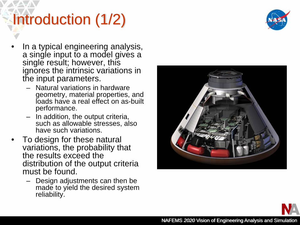
Introduction (1/2)• In a typical engineering analysis,

a single input to a model gives a single result; however, this ignores the intrinsic variations in the input parameters.– Natural variations in hardware

geometry, material properties, and loads have a real effect on as-built performance.

– In addition, the output criteria, such as allowable stresses, also have such variations.

• To design for these natural variations, the probability that the results exceed the distribution of the output criteria must be found.– Design adjustments can then be

made to yield the desired system reliability.


Introduction (2/2)• The Orion Crew Exploration

Vehicle (CEV) is part of the NASA Constellation Program to return humans to the moon and to serve as a building block to Mars and other destinations in the solar system.– It is similar in shape to the Apollo

spacecraft, but significantly larger, and will also be capable of carrying crew and cargo to the International Space Station.

– The figure depicts an exploded view of the Orion CEV, with the Heat Shield (HS) on the far right.

– The Heat Shield consists of individual ablator tiles bonded to a metallic carrier structure.

– http://www.nasa.gov/mission_pages/constellation/multimedia/orion_contract_images.html


Cielo Overview (1/2)• Goals:

– Enable “integrated modeling” via fundamentally-integrated thermal, structural, and optical aberration analytic capabilities.

– Overcome “Commercial Off-The-Shelf” (COTS) tool limitations.– Provide a platform for continuing methods and vertical application development.

• Status:– Six-year-plus development effort largely by team of former MSC/NASTRAN developers.– MATLAB hosted, modular, large model implementation (> 1M structural degrees of

freedom, tens of thousands of radiation exchange surfaces).– Extensible serial and parallel components (heterogeneous compute environment).– Under active development.

Diffuse View Factors Thermal Deformations Optical Aberrations


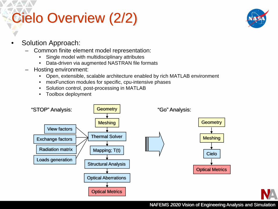
Cielo Overview (2/2)• Solution Approach:

– Common finite element model representation:• Single model with multidisciplinary attributes• Data-driven via augmented NASTRAN file formats

– Hosting environment:• Open, extensible, scalable architecture enabled by rich MATLAB environment• mexFunction modules for specific, cpu-intensive phases• Solution control, post-processing in MATLAB• Toolbox deployment

“STOP” Analysis: “Go” Analysis:

Geometry

Meshing

Cielo

Optical Metrics

Optical Metrics

Geometry

Meshing

Mapping; T(t)

Structural Analysis

Optical Aberrations

Thermal SolverView factors

Exchange factors

Radiation matrix

Loads generation


Cielo Architecture

Solnx

GUIx

Datax

Modx

Customuser components

HostLayer(MATLAB API)

Object-based Data Layer

GUI/results postprocessing

Solution sequences

Inputdata file

CADModeling

tools

View OpticsOrbit …Computationalmodules (serialor parallel)

Data API

MATLAB

Optional MATLAB

input


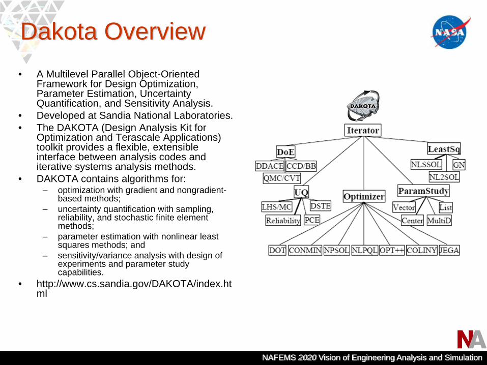
Dakota Overview• A Multilevel Parallel Object-Oriented

Framework for Design Optimization, Parameter Estimation, Uncertainty Quantification, and Sensitivity Analysis.

• Developed at Sandia National Laboratories.• The DAKOTA (Design Analysis Kit for

Optimization and Terascale Applications) toolkit provides a flexible, extensible interface between analysis codes and iterative systems analysis methods.

• DAKOTA contains algorithms for:– optimization with gradient and nongradient-

based methods;– uncertainty quantification with sampling,

reliability, and stochastic finite element methods;

– parameter estimation with nonlinear least squares methods; and

– sensitivity/variance analysis with design of experiments and parameter study capabilities.

• http://www.cs.sandia.gov/DAKOTA/index.html


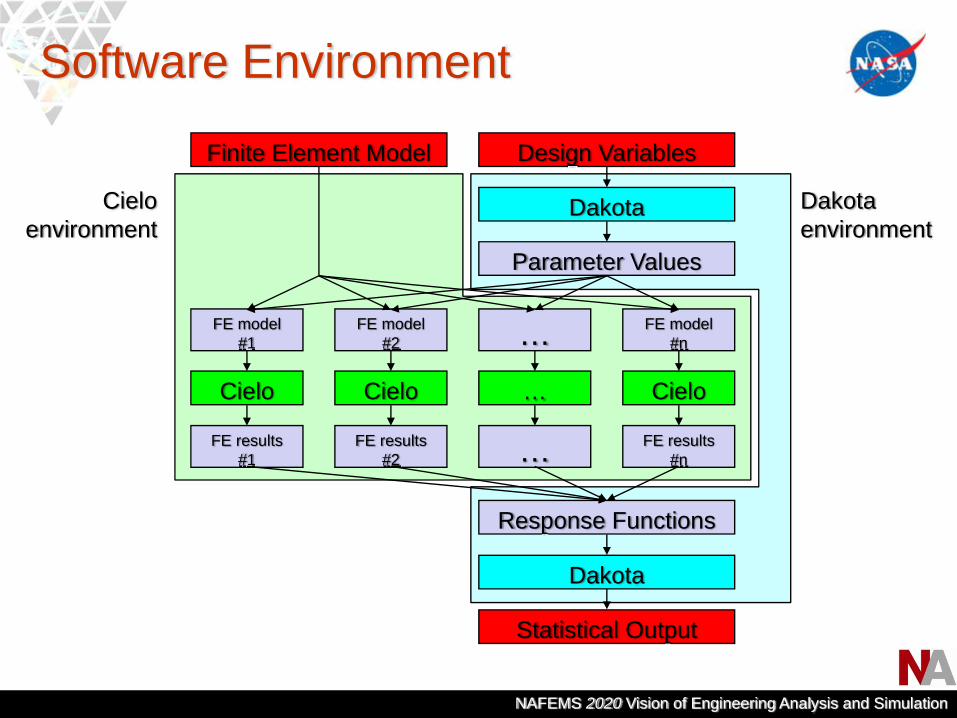
Software Environment

Dakota

Dakota

Statistical Output

Cielo…CieloCielo

Design VariablesFinite Element Model

FE model #n…FE model

#2FE model

#1

FE results #n…FE results

#2FE results

#1

Parameter Values

Response Functions

Cielo environment

Dakota environment


Orion CEV Heat Shield DetailPICA Blocks (365)

Compression Pads (6)

+Z

+Y

Carrier Structure dish regiongore panels

Carrier Structure shoulder

Compression Pad inserts

Main Seal (HS-BS joint)


Reentry Load Case Analysis

DisplacementMapping

Pressure Loadsfrom CBAERO

PressureMapping

PV Model

Temperature Loadsfrom FIAT

TemperatureMapping

Tile Model


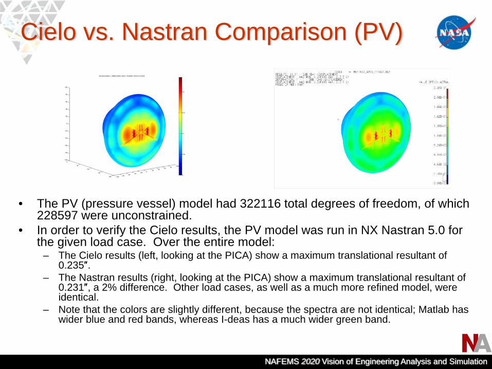
Cielo vs. Nastran Comparison (PV)

• The PV (pressure vessel) model had 322116 total degrees of freedom, of which 228597 were unconstrained.

• In order to verify the Cielo results, the PV model was run in NX Nastran 5.0 for the given load case. Over the entire model:

– The Cielo results (left, looking at the PICA) show a maximum translational resultant of 0.235″.

– The Nastran results (right, looking at the PICA) show a maximum translational resultant of 0.231″, a 2% difference. Other load cases, as well as a much more refined model, were identical.

– Note that the colors are slightly different, because the spectra are not identical; Matlab has wider blue and red bands, whereas I-deas has a much wider green band.


Cielo vs. Nastran Comparison (Tile)

• The PICA (phenolic impregnated carbon ablator) tile model had 219786 degrees of freedom, of which 104304 were unconstrained.

• The tile model was run in Cielo and NX Nastran 5.0 (SOL 106) with temperature-dependent material properties. On the tile:

– The Cielo results (left, looking at the PICA) show a maximum translational resultant of 0.0705″.

– The Nastran results (right, looking at the PICA) show a maximum translational resultant of 0.0705″, exact to the number of digits given.

– The individual displacement components (not shown) agree equally well.– Note that the colors are slightly different, because the spectra are not identical; Matlab has

wider blue and red bands, whereas I-deas has a much wider green band.


Uncertainty Quantification (1/5)• CS Design Variables:

– The CS (carrier structure) was divided into nine sandwich zones and two shoulder zones, which were used as design variables.

• normal_uncertain distribution of thicknesses with nominal mean and standard deviation of 5%.

– Factors were added to the external load cases from CBAERO.

• normal_uncertain distribution of factor of safety with nominal mean and standard deviation of 5%.

• Tile Design Variables– The PICA material properties are given

at a virgin, intermediate, and char temperatures and interpolated in between.

• normal_uncertain distribution of CTE’s, moduli, and temperatures with nominal means and standard deviations of 5%.

• Scaling was required for CTE’s in Dakota.


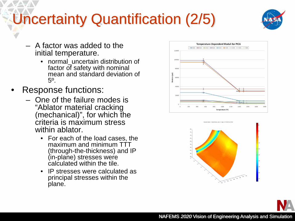
Uncertainty Quantification (2/5)– A factor was added to the

initial temperature.• normal_uncertain distribution of

factor of safety with nominal mean and standard deviation of 5º.

• Response functions:– One of the failure modes is

“Ablator material cracking (mechanical)”, for which the criteria is maximum stress within ablator.

• For each of the load cases, the maximum and minimum TTT (through-the-thickness) and IP (in-plane) stresses were calculated within the tile.

• IP stresses were calculated as principal stresses within the plane.


Uncertainty Quantification (3/5)• Various uncertainty quantification (UQ) analyses can be run using the

Cielo/Dakota environment:– Sampling methods (nond_sampling):

• Monte Carlo sampling (sample_type random) – traditional• Latin Hypercube sampling (sample_type lhs) – stratified sampling technique

• In addition to the sampling methods, there are also reliability methods in Dakota:– Based on probabilistic approaches that compute approximate response function

distribution statistics based on uncertain variable distributions.– Local reliability methods (nond_local_reliability):

• Mean value– Estimates statistics based on a single evaluation of response functions and gradients at

the means (MV).– Can have acceptable accuracy when response functions are nearly linear and

distributions are approximately Gaussian.• MPP search

– Solves an optimization problem to compute a most probable point (MPP) and then integrate to compute probabilities.

– Can use first or second order Taylor series approximation at a single point, with or without iterative expansion; multipoint approximations; or original response function with no approximations.


Uncertainty Quantification (4/5)• Forward algorithm of computing CDF probabilities for specified response

levels is the reliability index approach (RIA).• Inverse algorithm of computing response levels for specified CDF

probabilities is the performance measure approach (PMA).– Global reliability methods (nond_global_reliability):

• Designed to handle non-smooth and multimodal failure surfaces by creating global approximations.

• Accurately resolve a particular contour and then estimate probabilities using multimodal adaptive importance sampling.

– Does not depend on accurate gradient information.– Ability to locate multiple failure points.– Because of adaptive nature, often uses only a single processor.

– Available output:• All reliability methods output either the probabilities (RIA) or the response

levels (PMA).• In addition, the MV methods output estimated means and standard

deviation along with importance factors:– For independent random variables, importance factors are computed

for each of the uncertain variables.


Uncertainty Quantification (5/5)

• Sampling analyses were run on a four-processor Sun Ultra 40 workstation at JPL:– Dakota drives the Cielo analyses:

• Supplies files of design variables, which are integrated into bulk data files.• Starts Matlab sessions for Cielo, which may be sequential or simultaneous.• Retrieves files of response functions, which are written by post-processing.

– Dakota can actually run Matlab directly, bypassing the text files, but this capability has not yet been used.

– Up to four Cielo analyses can run simultaneously on the Sun Ultra 40.– Dakota uncertainty analysis required about 77 hours for 1000 Cielo

finite element analyses.• Reliability analyses were also run on the Sun Ultra 40 at JPL:

– Local reliability analyses using the mean-value method, both RIA and PMA, were run.

• For RIA, the ultimate material quartiles were input as response levels.• For PMA, the percentages into the tails of the CDF’s were input.

– Each took less than ten hours with four processors for the given load case.


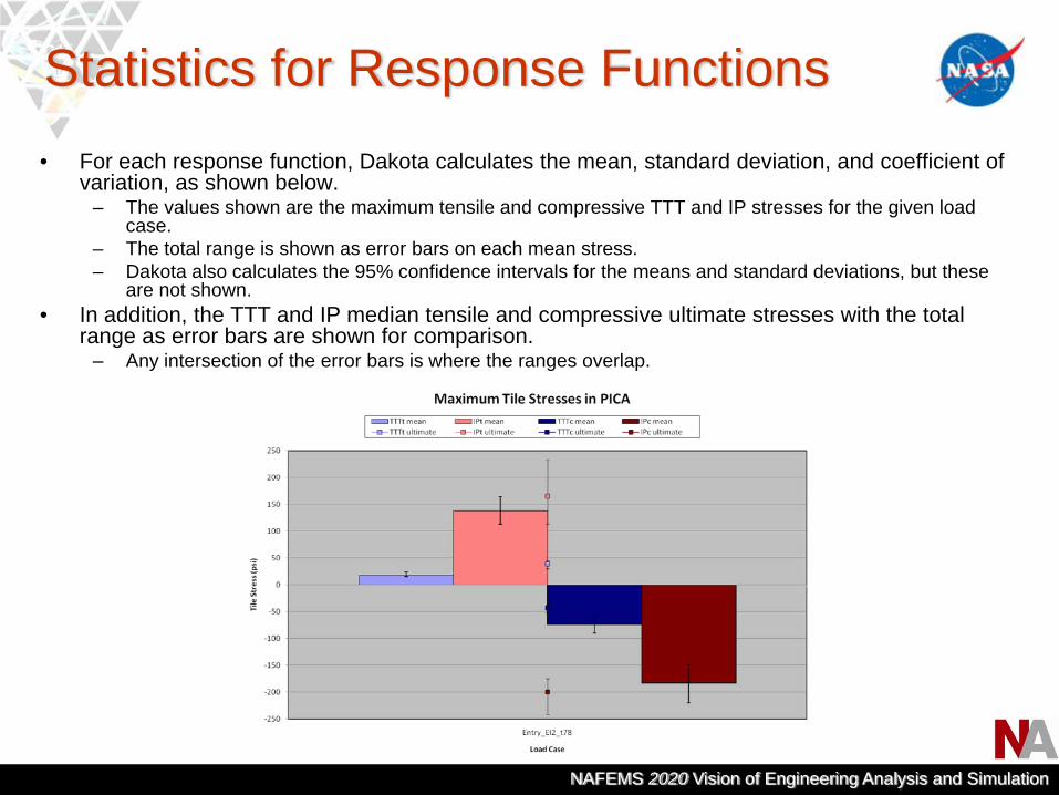
Statistics for Response Functions• For each response function, Dakota calculates the mean, standard deviation, and coefficient of

variation, as shown below.– The values shown are the maximum tensile and compressive TTT and IP stresses for the given load

case.– The total range is shown as error bars on each mean stress.– Dakota also calculates the 95% confidence intervals for the means and standard deviations, but these

are not shown.• In addition, the TTT and IP median tensile and compressive ultimate stresses with the total

range as error bars are shown for comparison.– Any intersection of the error bars is where the ranges overlap.


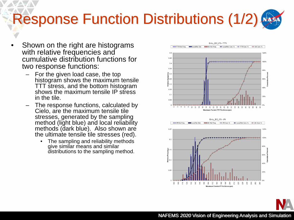
Response Function Distributions (1/2)• Shown on the right are histograms

with relative frequencies and cumulative distribution functions for two response functions:

– For the given load case, the top histogram shows the maximum tensile TTT stress, and the bottom histogram shows the maximum tensile IP stress in the tile.

– The response functions, calculated by Cielo, are the maximum tensile tile stresses, generated by the sampling method (light blue) and local reliability methods (dark blue). Also shown are the ultimate tensile tile stresses (red).

• The sampling and reliability methods give similar means and similar distributions to the sampling method.


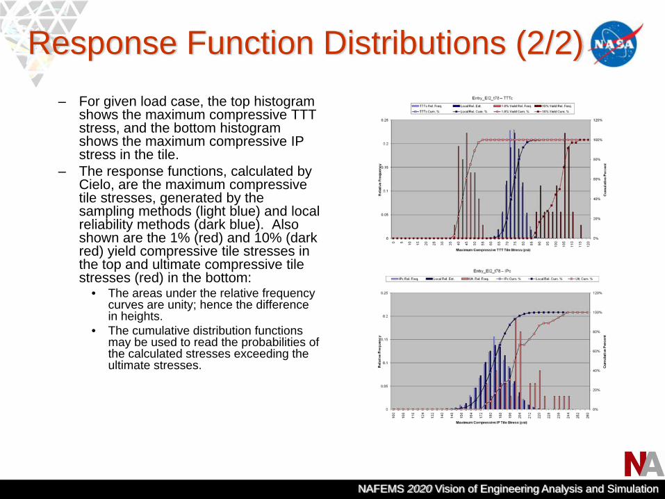
Response Function Distributions (2/2)– For given load case, the top histogram

shows the maximum compressive TTT stress, and the bottom histogram shows the maximum compressive IP stress in the tile.

– The response functions, calculated by Cielo, are the maximum compressive tile stresses, generated by the sampling methods (light blue) and local reliability methods (dark blue). Also shown are the 1% (red) and 10% (dark red) yield compressive tile stresses in the top and ultimate compressive tile stresses (red) in the bottom:

• The areas under the relative frequency curves are unity; hence the difference in heights.

• The cumulative distribution functions may be used to read the probabilities of the calculated stresses exceeding the ultimate stresses.


Probabilities for Response Functions• If requested, Dakota calculates the cumulative distribution functions for each

response function.– Probabilities and reliabilities may be calculated from the response levels, or vice versa.

• The quartiles for the TTT and IP ultimate stresses were used as the response levels to calculate the probability levels, as shown below for the tile.

• The chart show the probability for the response functions to be below each quartile.

– The four quartiles of the tensile and compressive ultimate stresses, along with below the minimum and above the maximum, are color-coded for each stress.


Simple Correlation Matrix• Dakota calculates four correlation matrices:

– Simple and partial “raw”, where “raw” refers to actual input and output data.– Simple and partial “ranked”, where “ranked” refers to input and output data in ascending

order.• The simple correlation matrix is shown below.

– The correlations between the design variables themselves show that they are chosen to be uncorrelated.

– The correlations between the design variables and the response functions show which design variables have the largest effect. These are color-coded from the most positive (green) to most negative (red) correlations, with uncorrelated as yellow.


Importance Factors• The importance factors are

shown on the right for the RIA and PMA local reliability methods, respectively. – For each response function, the

factors add up to unity.– The two methods give identical

results.– Though difficult to see with 60

design variables, the top 4 are:• aip_a2 (dark red in all)• k33_k3 (light pink in ip_c)• k33_k1 (light green in ip_t)• k11_k1 (dark green in ttt_c)

– The values agree qualitatively with those in the simple correlation matrix for the sampling method.

– Note that none of the PV design variables are noticeable.


Summary

• Two software packages, Cielo from JPL and Dakota from Sandia, were coupled to create an environment for performing uncertainty quantification.

• This environment was applied to the Orion CEV Heat Shield:– Design variables consisted of:

• geometrical thicknesses and load factors in the PV; and• temperature-dependent material properties in the tile.

– Response functions consisted of:• TTT and IP stresses in the tile.

• Given the distributions on the design variables, such as those determined by machining tolerances and material testing, distributions of the output stresses were calculated.

• Calculating the probabilities that the outputs with their distributions exceed the failure criteria with their distributions provides a more sound basis for making engineering decisions.


Acknowledgments

• The authors are grateful for the contributions of Greg Moore, Mike Chainyk, Claus Hoff, and Eric Larour at the Jet Propulsion Laboratory for Cielo development; and of Kenneth R. Hamm Jr., Structures and Analysis Lead, and Alberto Makino, Mechanical Engineer and Structural Analyst at the NASA Ames Research Center, and David F. Moore, Aerospace Engineer at the NASA Langley Research Center for model development.

• Part of the research described in this presentation was carried out at the Jet Propulsion Laboratory, California Institute of Technology, under a contract with the National Aeronautics and Space Administration. Reference herein to any specific commercial product, process, or service by trade name, trademark, manufacturer, or otherwise, does not constitute or imply its endorsement by the United States Government or the Jet Propulsion Laboratory, California Institute of Technology.

• This presentation has been cleared for unlimited release (JPL CL#08-3885). This clearance is valid for US and foreign release.


References• Contributing references:

– http://www.nasa.gov/mission_pages/constellation/multimedia/orion_contract_images.html

– Greg Moore, Mike Chainyk, Claus Hoff, Eric Larour, John Schiermeier, “Cielo: An Open Environment for Analysis-Driven Systems Engineering”, AIAA Space 2007, Long Beach, Calif., September 18-20, 2007.

– http://www.cs.sandia.gov/DAKOTA/index.html– Mitch S. Eldred, et.al., “DAKOTA Version 4.1 User’s Manual”, Sandia National

Laboratories, September, 2007.• Additional references:

– Claus Hoff, Mike Chainyk, Eric Larour, Greg Moore, John Schiermeier, “Modeling and Simulation of the SIM TOM3 Testbed: A V&V Exercise Using Cielo”, WCCM 2008, Venice, Italy, July 2, 2008.

– Mike Chainyk, Claus Hoff, Eric Larour, Greg Moore, John Schiermeier, “Cielo: An Open Environment for Multi-Physics Simulation Applied to Thermal, Structural and Optical Aberration Analysis of Large Space Based Instruments”, NAFEMS World Congress 2007, Vancouver, Canada May 22-25, 2007.

– Eric Larour, Eric Rignot, “A new penalty based approach to large scale modeling of Antarctica using 2d-3d lower and higher order finite elements”, Los Alamos National Laboratory meeting: Building a next generation community ice sheet model, August 18, 2008.


Author Contact Information

• John E. SchiermeierSenior Member Technical StaffMS 157-316Jet Propulsion LaboratoryCalifornia Institute of Technology4800 Oak Grove DrivePasadena, California [email protected]

• Jeremy C. Vander KamAerospace EngineerMS 258-1NASA Ames Research CenterMoffett Field, California [email protected]

Documents

Uncertainty Quantification for the Orion Crew Exploration ... · Uncertainty Quantification for the Orion Crew Exploration Vehicle Heat Shield Using Cielo and Dakota John E. Schiermeier