Embed Size (px)
Citation preview
1
Institutt for marin teknikk
Error and Uncertainty AnalysisExperimental Methods in Marine Hydrodynamics
Week 37
Objectives:• Understand the importance of getting a measure of the uncertainty of an
experimental result• Learn how to find the uncertainty of the outcome of an experiment
Covers chapter 12 in the Lecture Notes
2
Institutt for marin teknikk
Contents
• What is the difference between error and uncertainty?• Introduction of some basic concepts• Why uncertainty analysis?• How to determine the uncertainty of measurements?• Error propagation and sensitivity to errors on final results• Calculation of total uncertainty of experiments • Impact on final conclusions?

3
Institutt for marin teknikk
Measured model resistance in lab 1 2011

4
Institutt for marin teknikk
Measured model resistance comparison

5
Institutt for marin teknikk
Residual Resistance Coefficient

6
Institutt for marin teknikk
Residual Resistance Coefficient Comparison

7
Institutt for marin teknikk
Error
Suppose we know the true value
Then, this is the error of a single measurement
The problem is that we usually don’t know the true value(That is why we do the experiment)

8
Institutt for marin teknikk
Definition of error and uncertainty
• Error is the difference between the measured value and the true value:
|Error| = | measured value – true value |
– Problem: The true value is very seldom known
• Uncertainty is the statistical representation of error → the expected error of a measurement
• Confidence interval: The range of probable values of an experiment– Example: A 95% confidence interval of 2 N means that 95% of all
readings of a particular measurement will be within 2 N from the ”true” value

9
Institutt for marin teknikk
Measured model resistance comparison

10
Institutt for marin teknikk
Bias and Precision Error
• Precision error: ”scatter” in the experimental results– Found from repeated measurements
• Bias error: Systematic errors, not found from repeated measurements
• Replication level: How much of an experimental set-up that is repeated when finding the precision error– Example of different repetition levels of a resistance test:
1. Only the test itself (running the same speed twice)2. Repeat also the connection to the carriage3. Repeat also the ballasting of the model4. Making a new model, testing in the same tank5. Making a new model at another towing tank, testing in a different tank
(facility bias)

11
Institutt for marin teknikk
Results of repeated resistance tests
1
1.2
1.4
1.6
1.8
2
2.2
0.1 0.15 0.2 0.25 0.3 0.35Froude number Fn [-]
Res
idua
l res
ista
nce
CR*1
000
[-]Group 1 2004Group 2 2004Group 3 2004Group 4 2004Group 3&4 2005Group 1&2 2005All groups 2006
12
Institutt for marin teknikk
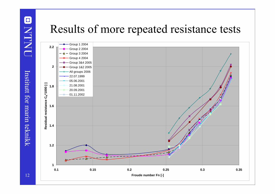
Results of more repeated resistance tests
1
1.2
1.4
1.6
1.8
2
2.2
0.1 0.15 0.2 0.25 0.3 0.35Froude number Fn [-]
Res
idua
l res
ista
nce
CR*1
000
[-]Group 1 2004Group 2 2004Group 3 2004Group 4 2004Group 3&4 2005Group 1&2 2005All groups 200622.07.199905.06.200121.08.200120.09.200101.11.2002

13
Institutt for marin teknikk
Why do we want to know the uncertainty of an experimental result?

14
Institutt for marin teknikk
5000
7000
9000
11000
13000
15000
17000
19000
21000
23000
17 18 19 20 21 22 23 24 25
Ship speed [knots]
Tota
l Bra
ke P
ower
[kW
]
Prediction from model testContractual condition
Example: Speed prediction of a car carrier
Cancellation limit
Contract: The ship shall do 23 knots at a brake power of 20 000 kW

15
Institutt for marin teknikk
Uncertainty of PB calculated to 2%
5000
7000
9000
11000
13000
15000
17000
19000
21000
23000
25000
17 18 19 20 21 22 23 24 25
Ship speed [knots]
Tota
l Bra
ke P
ower
[kW
]
Prediction from model testContractual condition
Uncertainty: 2% on PB

16
Institutt for marin teknikk
Uncertainty of PB calculated to 10%
5000
7000
9000
11000
13000
15000
17000
19000
21000
23000
25000
17 18 19 20 21 22 23 24 25
Ship speed [knots]
Tota
l Bra
ke P
ower
[kW
]
Prediction from model testContractual condition
Uncertainty: 10% on PB
In this case there might be a problem!

17
Institutt for marin teknikk
Example 2a: Comparison of experimentally and numerically calculated RAO in heave acc.
Response amplitude operators
accelerations at pos AP
0.00
0.20
0.40
0.60
0.80
1.00
1.20
1.40
1.60
1.80
0 5 10 15 20 25 30
Wave period [s]
RAO Heave acc.3 / a [m/s²]
VERESModel testModel test, mean
Conclusion: Calculations not in agreement with experiments
Uncertainty: 2.08%

18
Institutt for marin teknikk
Example 2b: Comparison of experimentally and numerically calculated RAO in heave acc.
Response amplitude operatorsaccelerations at pos AP
0.00
0.50
1.00
1.50
2.00
2.50
0 5 10 15 20 25 30
Wave period [s]
RAO Heave acc.3 / a [m/s²]
VERESModel testModel test, mean
Conclusion: Calculations in agreement with experiments
Uncertainty: 30%

19
Institutt for marin teknikk
mean true
1.0-0.95
-0.2
0
0.2
0.4
0.6
0.8
1
1.2
1.4
1.6
1.8
2
-0.5 0 0.5 1 1.5 2 2.5 3 3.5
Result X
Gau
ssia
n di
strib
utio
nf(X
)Bias error
Confidence interval
Calculation of precision error
2
2212
X
f X e
20
Institutt for marin teknikk
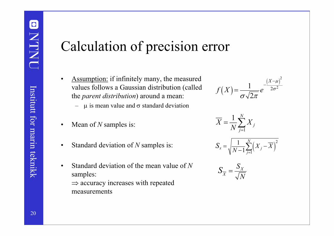
Calculation of precision error
• Assumption: if infinitely many, the measured values follows a Gaussian distribution (called the parent distribution) around a mean:
– is mean value and standard deviation
• Mean of N samples is:
• Standard deviation of N samples is:
• Standard deviation of the mean value of Nsamples: accuracy increases with repeated measurements
2221
2
X
f X e
1
1 N
jj
X XN
21
11
N
x jj
X XN
S
XX
SN
S

21
Institutt for marin teknikk
Calculation of precision error
• For the parent distribution the confidence interval of a sample is given by:
– t 1.96 for a normal distribution– is the confidence interval, = 0.95 when t 1.96
• For a finite number of samples N, σ and t of the parent distribution is unknown
• Re-write eq. 1 as:
• Then is random and follow a Student’s t distribution with N-1 degrees of freedom
• The precision limit of a sample is now easily found from
Prob j jX t X t
Prob j
x
XS
t t
j
X
X
S
x xP t S

22
Institutt for marin teknikk
The weight t for estimating confidence intervals using Student’s t distribution
0
1
2
3
4
5
6
7
8
0 5 10 15 20 25 30
Degrees of freedom (N-1)
Wei
ght t
95% confidence99% confidence

23
Institutt for marin teknikk
Finding the precision limit
• The precision limit of a sample:
• The precision limit of the average of N samples:
• Note that more than one sample is needed to calculate Sx:
Repeated measurements are required to calculate the precision limit of a single sample
Repeated measurements is a good (but time-consuming) way of decreasing the precision error of the results
x xP t S
XX
SP tN
21
11
N
x jj
X XN
S

24
Institutt for marin teknikk
0
1
2
3
4
5
6
7
8
0 5 10 15 20 25 30
Degrees of freedom (N-1)
Wei
ght t
95% confidence99% confidence
Typical number of repeated tests:
25
Institutt for marin teknikk
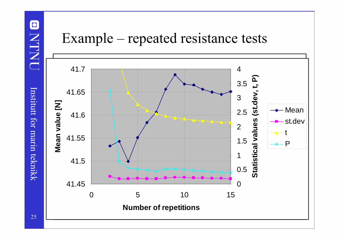
Example – repeated resistance testsRepeated resistance test with a conventional ship
model
41.341.441.541.641.741.841.9
4242.1
1.7015 1.702 1.7025 1.703 1.7035 1.704 1.7045 1.705 1.7055
Model speed Vm [N]
Mod
el re
sist
ance
RTm
[N]
41.45
41.5
41.55
41.6
41.65
41.7
0 5 10 15
Number of repetitions
Mea
n va
lue
[N]
0
0.5
1
1.5
2
2.5
3
3.5
4
Stat
istic
al v
alue
s (s
t.dev
, t, P
)
Meanst.devtP

26
Institutt for marin teknikk
Repeated tests in practice
1. Repeat all test conditions to reduce the uncertainty of the results– Too time consuming (and expensive) to be done in practice (in marine
hydrodynamics), except on some special research projects2. Repeat one (or a few carefully selected) test conditions to calculate the
precision error– Recommended practice in all research projects– Typically not done in routine commercial verification tests
3. Do a thorough uncertainty analysis, including repeated tests, of a typical standard tests (for instance resistance), and use the results as being representative for all standard tests of the same type• Recommended practice in standardized commercial testing

27
Institutt for marin teknikk
Chauvenet’s criterion for rejecting outliers
1 12 (1 )chauvenett F p
j xchauvenetX X St
Reject samples with larger deviation from the mean than given by:
F is the cumulative density function of the normal distributionp=1-1/(2N)

28
Institutt for marin teknikk
Estimating Bias Errors
• Can not be found from repeated tests• No standard way of calculating bias errors
– That’s why we say ”estimating”• Examples of bias errors:
– Calibration factors of the sensors• The bias error can be estimated from the precision error of the calibration
factor– Geometrical accuracy of a ship model
• Find the geometrical accuracy (for instance by control measurements)• Estimate the sensitivity of the measurement results from the geometrical
deviations (that is the hard part!)– Inaccurate calibration of (wave) environment– Tank wall effects
• Blockage (it is a pure bias error)• Wave reflections (can give both bias and precision)
29
Institutt for marin teknikk
Reducing bias errors
• Careful calibration of sensors and environment• Well-designed test set-up• Accurate manufacture of model• Careful installation of the model• Increase the replication level• Correlation
– Empirically based correction factors

30
Institutt for marin teknikk
What is the uncertainty of the final end result?
Example:• We want to find the uncertainty of the full-scale speed-power
prediction of our car carrier• Assume we have found the uncertainty of the model resistance
measurement and of the measurement of model propeller thrust and torque from repeated measurements (and by estimating bias errors)
• How do we find the uncertainty of the final prediction in full scale?
Two key concepts:– Data reduction equations– Error Propagation
31
Institutt for marin teknikk
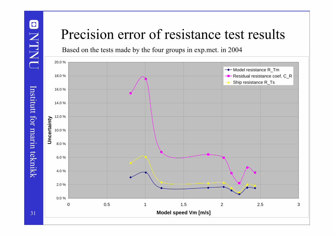
Precision error of resistance test results
0.0 %
2.0 %
4.0 %
6.0 %
8.0 %
10.0 %
12.0 %
14.0 %
16.0 %
18.0 %
20.0 %
0 0.5 1 1.5 2 2.5 3
Model speed Vm [m/s]
Unc
erta
inty
Model resistance R_TmResidual resistance coef. C_RShip resistance R_Ts
Based on the tests made by the four groups in exp.met. in 2004

32
Institutt for marin teknikk
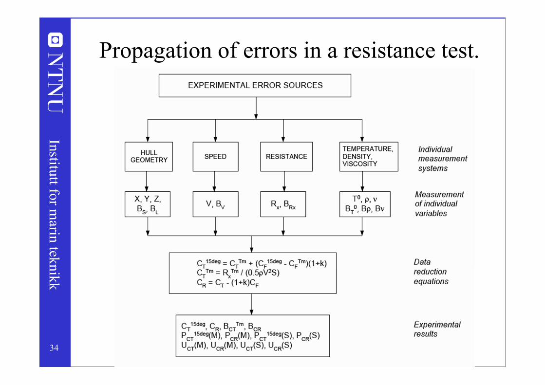
Data reduction equations
The mathematical equations describing the conversion from test result to final result
• The data reduction can in general be written as:• Taylor-expansion of the data reduction equation gives:
• The influence coefficient is defined as:
• The elemental error is then:
1 2, ,..., ,NX f Y Y Y
1
1
22 3
21 ( )2
N
i i
N
i i
i i ii
i
X XX X Y Y O YY YXX YY
i
i
XY
i i ii
iY YXe Y

33
Institutt for marin teknikk
Error propagation
• Assuming elemental error sources are independent, total error is found by summation:
• Total bias and precision errors are determined independently. Total error is found as:
– For 95% coverage
– For 99% coverage
2
1
N
ii
e e
2 2BSe e e
S Be ee
34
Institutt for marin teknikk
Propagation of errors in a resistance test.

35
Institutt for marin teknikk
Monte-Carlo simulation
Data reduction equations
Mea
sure
d va
riabl
es
Final result
Select range of variation for each “measured” variableCreate many (typically 10 000) randomly different sets of “measured” variables Gives you 10 000 slightly different final results
Analysis of the variation of final result, compared to the variation of inputs, shows the sensitivity of uncertainty in measured values of the final result Useful technique when the data reduction process is complicated

36
Institutt for marin teknikk
Steps in an uncertainty analysis
1. Identify all error sources2. Determine the individual precision and bias errors for each error
source3. Determine the sensitivity of the end result to error sources4. Create the total precision interval5. Create the total bias uncertainty6. Combine the total bias and precision7. Declare results from steps 4-6 separately in the report

37
Institutt for marin teknikk
Summary of the uncertainty analysis
• We always need knowledge about the uncertainty of an experimental result– Often, this “knowledge” is based on “gut feeling”, experience, or a crude order-of-
magnitude estimate– Increasingly, there is a demand for a formal analysis. Examples:
• When verifying numerical calculation methods by comparison with experiments• When it is very important to know that the experimental result is true within a known
uncertainty band• Error vs. Uncertainty:
– Error is the actual difference between a result and the true value– Uncertainty is the expected error – calculated based on statistics
• Problem: We don’t know the true value (that’s why we do the experiment!)• Error estimates are commonly divided in two categories:
– Precision errors – found from the scatter in repeated measurements– Bias errors – systematic errors, that can not be found from repeated measurements
• To find the uncertainty of the final result (for instance ship resistance) one needs to consider how the experimental error propagates through the data analysis (error propagation)
– We have seen how to use the data reduction equations to set up an analysis of the error propagation

38
Institutt for marin teknikk
Scale effects and other error sources

39
Institutt for marin teknikk
How can the accuracy be increased?
• Improve calibration procedures– More careful– Include more of the test set-up in the calibration– Non-linear calibration relation
• Change to more accurate transducers– More expensive– More sensitive (but then usually less robust)
• Re-design test set-up– For instance using larger model
• More careful test execution– For instance longer waiting times between runs
• Repeated measurements– Accuracy increases with √N

40
Institutt for marin teknikk
Bias Error Sources
• Scale effects• Model inaccuracies• Errors in test set-up• Calibration errors• Errors due to environmental modeling• Wave parameters and spectral shape• Tank wall effects

41
Institutt for marin teknikk
Model inaccuracies
• Inaccurate draught/ballasting– Error is minimized by ballasting to correct weight, not to specified draught
• Model surface too rough– Poor paintwork– The surface finish deteriorates with time
It is common for the resistance to increase about 2% after one year storage• Inaccurate shape (production errors)• Model deformations
– Could be the reason for the fact that model resistance tend to increase with time

42
Institutt for marin teknikk
Errors in test set-up
• Influence of Model Connections (Example: resistance test)– Towed at a position too high in the model– Model not correctly aligned– External forces acting, for instance strain in cables– The force transducer might not measure the force exactly in the horizontal
direction• Uncertainty of calibrations
– The uncertainty in calibrations can be calculated• Systematic errors in measurement systems
– Use end-to-end calibrations to find and correct such error(End-to-end calibrations means to calibrate the entire test set-up)

43
Institutt for marin teknikk
Errors due to environmental modeling• Wave parameters and spectral shape
– Always calibrate the waves used in an experiment– Use the results of the calibrations rather than the specified wave– Quality of wave makers and wave generation system is important!– Wave reflections from tank walls is an important problem
• Effective wave damping is important• Reflection will often limit the length of measurement
• Seiching and temperature layers in the water– Might turn up also as precision errors
• For offshore testing, quality of modeled current is often critical
Seiching:Standing wave in the tank or basin
Termperature layers:Might cause internal waves, since the different layers have different density

44
Institutt for marin teknikk
Seiching – standing waves in the tank
Length Ltank
Depth h
Amplitude a
Horisontal velocity Vx
)sin()cos( kxta
)sin()sin( kxtgkV ax
hgLT Tank
2
•Wave elevation:
•Horizontal velocity:
•Wave period:

45
Institutt for marin teknikk
Error from seishing on total resistance- Example from the large towing tank
•Wave amplitude a = 1 cm
•Horizontal max velocity Vx = 0.03 m/s
•Carriage speed Vm = 1.5 m/s
•Total resistance: ½V2
•Induced max. Error: 4%

46
Institutt for marin teknikk
Tank wall effects• Usually, we want our test to represent our model in the open sea• When we do the experiments in a model basin there will inevitably be
boundaries• We must make sure that these boundaries doesn’t influence the results• Types of influence:
– Blockage – influencing steady velocity and pressure around a forward-moving model
– Wave reflections• Generated waves are reflected from imperfect wave damping devices• Reflected and radiated waves from the model are reflected from tank walls and
wave maker back to the model

47
Institutt for marin teknikk
Tank wall effects - Blockage
• Effective speed is increased due to the presence of the model
Blockage correction
0
0.001
0.002
0.003
0.004
0.005
0.006
0.007
0.008
0.009
0.01
0 0.5 1 1.5 2 2.5 3 3.5
Vm [m/s]
Velo
city
cor
rect
ion
fact
or
V/V
[-]
ScottSchuster
48
Institutt for marin teknikk
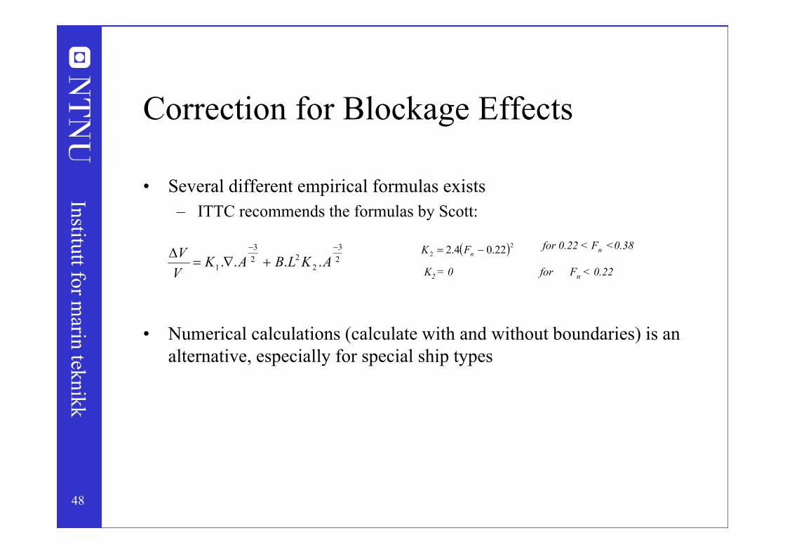
Correction for Blockage Effects
• Several different empirical formulas exists– ITTC recommends the formulas by Scott:
• Numerical calculations (calculate with and without boundaries) is an alternative, especially for special ship types
23
222
3
1 ....
AKLBAKVV 2
2 22.04.2 nFK for 0.22 < Fn <0.38
K2 = 0 for Fn < 0.22

49
Institutt for marin teknikk
Tank wall effects - Wave reflections
Comparison between numerical and experimental results for first order vertical wave forces on a hemisphere – Effect of tank wall interference

50
Institutt for marin teknikk
Wave reflections from moving models
•Radiated waves=created by model motions
•Diffracted waves=incoming waves reflected • by the model
2ge
gc
•Wave group speed:
2M gM M
w e
L cL L gUcrit
t B B
•This is why you should not run zero speed tests in a towing tank!

51
Institutt for marin teknikk
Ways to minimize the wave reflection problem for zero and low speed• Keep the model small relative to the size of the basin (or width of tank)• Install effective wave damping devices
– Hardly possible along the sides of a towing tank– Even the best wave beaches aren’t 100% effective at all wave lengths
• Limit the duration of the test– Not much of an alternative for irregular wave conditions– To be considered for regular wave and impulse wave tests

52
Institutt for marin teknikk
Wave reflections – in labtest 5
The carriage stops Wave reflections start

53
Institutt for marin teknikk
Scale Effects
• Reynolds effects– Frictional resistance– Boundary layer thickness– Different flow separation pattern
• Cavitation– Important only for performance of foils and propulsors
• Surface tension, spray, Weber number– Gives a limit for minimum model size
• Air pressure ratio– The atmospheric pressure is not scaled– Relevant for seakeeping testing of ships with air cushion

54
Institutt for marin teknikk
Reynolds scale effects - Forces
• Froude scaling requires:
• When C is dependent on scale we are most likely having a Reynolds scale effect
212
equal in model and full scaleFCV A
(When V is scaled by square root of scale ratio)

55
Institutt for marin teknikk
Reynolds Scale Effects – Skin Friction

56
Institutt for marin teknikk
Correcting for Reynolds scale effect on full scale resistance

57
Institutt for marin teknikk
Reynolds Scale Effect on Lift of Foils
3
1
2 2
3
1

58
Institutt for marin teknikk
Wake scale effect
Model Ship
Reynolds number
Boundary layer thickness
0.04 ( 0.04 ) Fs Fs m
Fm
C Cw t w t
C

59
Institutt for marin teknikk
Reynolds Scale Effects – Drag forces
Squared cylinder
221 DUCdF DD
Circular cylinder

60
Institutt for marin teknikk
Reynolds scale effects on propellers
• Scale effect on blade drag → propeller torque → KQ
– Due to Rn-effect on skin friction– Possibly due to flow separation
• Scale effect on blade lift→ propeller thrust → KT
– Rn-effect on foil lift• Minimize effect by requiring model Rn>2·105
• Established correction method (ITTC’78 method ):
DZc
DPCCKK DSDMTPMTPS
.3.0
DZcCCKK DSDMQMQS.25.0

61
Institutt for marin teknikk
Reynolds scale effects – short summary
• On skin friction– Established correction methods exists (friction lines)
• On pressure drag – Depends on flow separation and vortex generation– Established correction methods exist for simple cases (geometries)
• On flow fields (f.i. boundary layers)– Established correction methods exists only for simple cases– CFD (RANS codes) might play an increasing role
• On lift from lifting surfaces (foils and propellers)– Commonly neglected effect– Little data exists– Depends on details in the geometry -> boundary layer development
62
Institutt for marin teknikk
Summary of error sources
• Discussed sources of precision error• Discussed sources of bias error:
– Scale effects– Model inaccuracies– Errors in test set-up– Calibration errors– Errors due to environmental modeling– Wave parameters and spectral shape– Tank wall effects