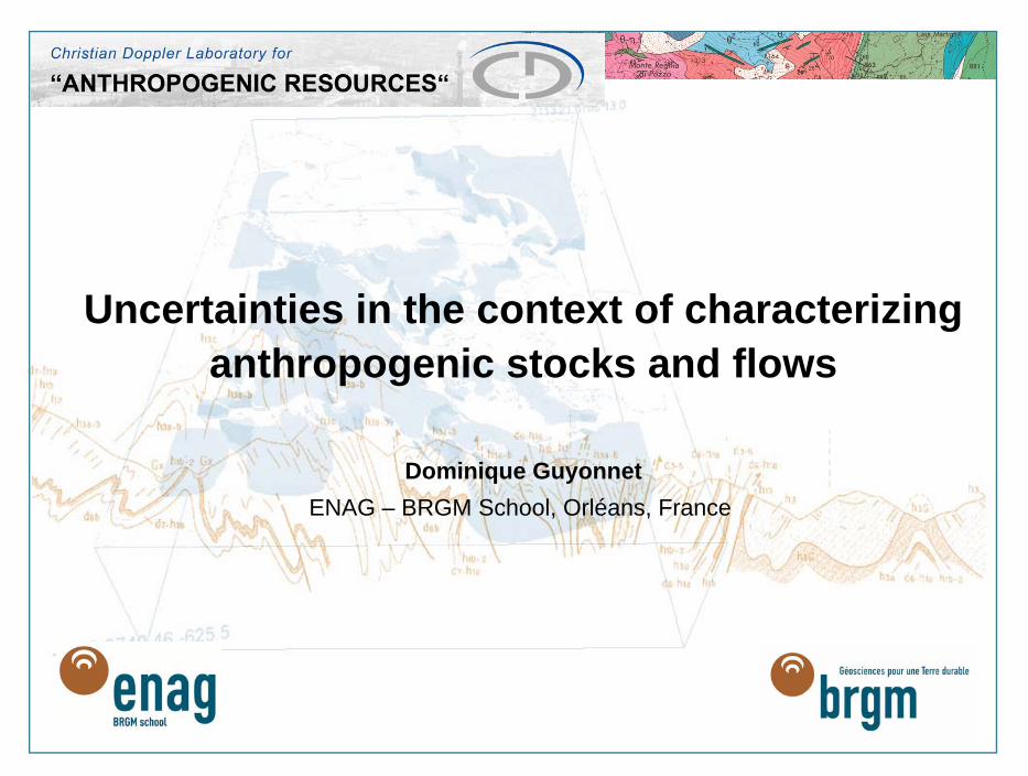
Uncertainties in the context of characterizing anthropogenic stocks and flows

Dominique GuyonnetENAG – BRGM School, Orléans, France

> 2

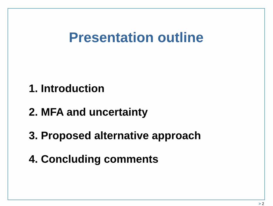
Presentation outline

1. Introduction

2. MFA and uncertainty

3. Proposed alternative approach

4. Concluding comments

> 3

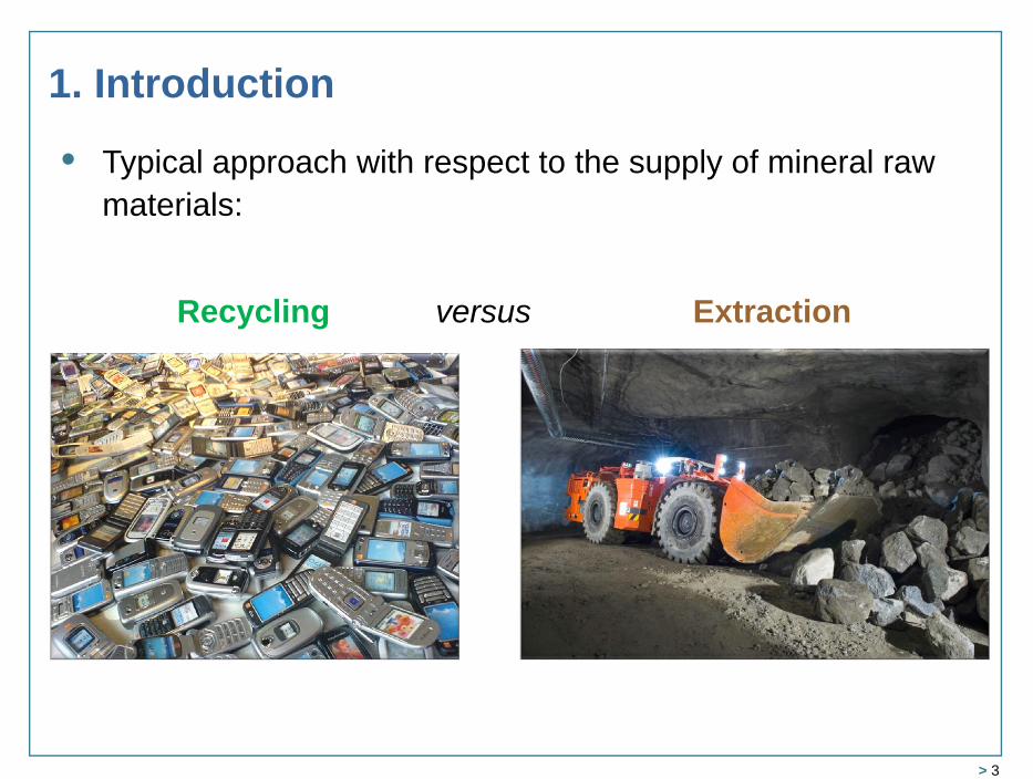
• Typical approach with respect to the supply of mineral raw materials:

Recycling Extractionversus

1. Introduction

> 4

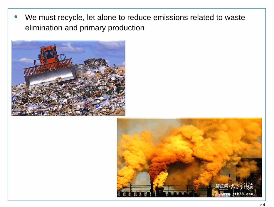
• We must recycle, let alone to reduce emissions related to waste elimination and primary production

> 5

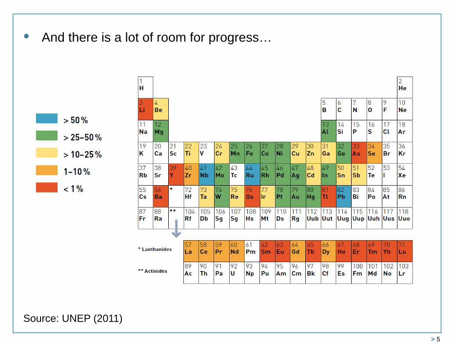
• And there is a lot of room for progress…

Source: UNEP (2011)

> 6

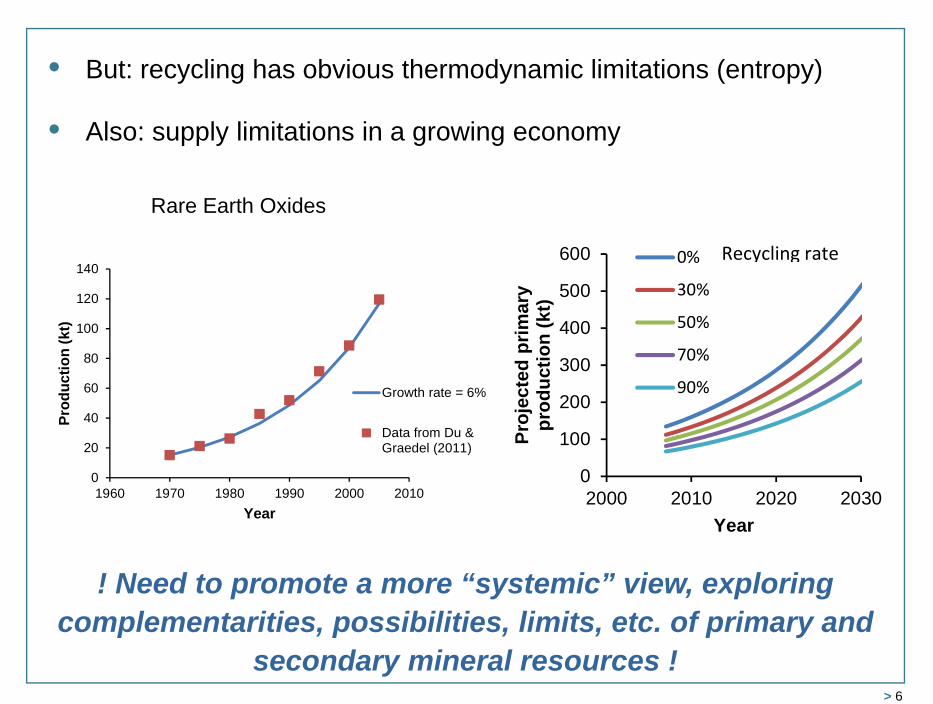
• But: recycling has obvious thermodynamic limitations (entropy)

• Also: supply limitations in a growing economy

Rare Earth Oxides

! Need to promote a more “systemic” view, exploring complementarities, possibilities, limits, etc. of primary and

secondary mineral resources !

0

20

40

60

80

100

120

140

1960 1970 1980 1990 2000 2010

Prod

uctio

n (k

t)

Year

Growth rate = 6%

Data from Du &Graedel (2011)

0

20

40

60

80

100

120

140

1960 1970 1980 1990 2000 2010

Prod

uctio

n (k

t)

Year

Growth rate = 6%

Data from Du &Graedel (2011)

0

100

200

300

400

500

600

2000 2010 2020 2030Pr

ojec

ted

prim

ary

prod

uctio

n (k

t)Year

0%

30%

50%

70%

90%

Recycling rate

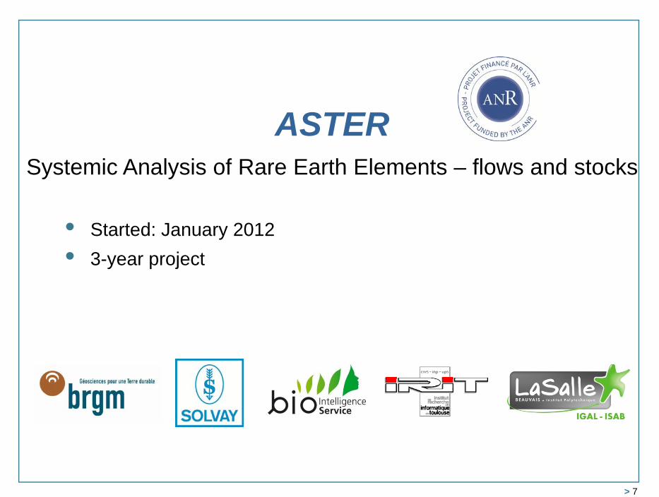
ASTERSystemic Analysis of Rare Earth Elements – flows and stocks

> 7

• Started: January 2012• 3-year project

> 8

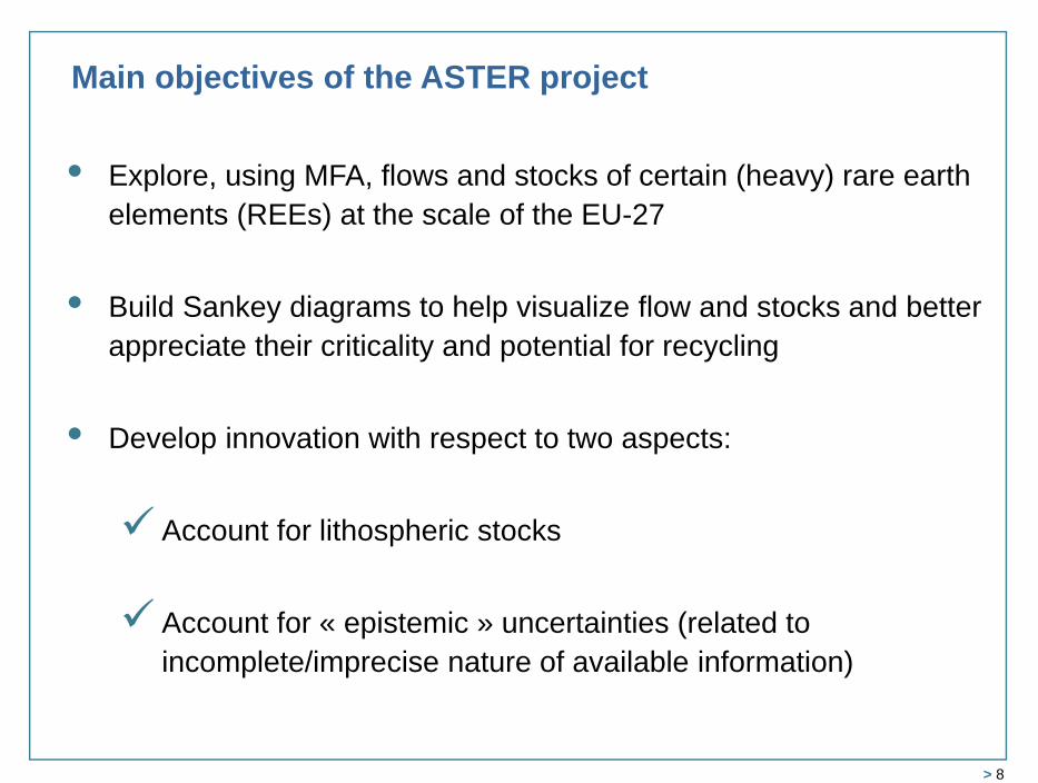
Main objectives of the ASTER project

• Explore, using MFA, flows and stocks of certain (heavy) rare earth elements (REEs) at the scale of the EU-27

• Build Sankey diagrams to help visualize flow and stocks and better appreciate their criticality and potential for recycling

• Develop innovation with respect to two aspects:

Account for lithospheric stocks

Account for « epistemic » uncertainties (related to incomplete/imprecise nature of available information)

> 9

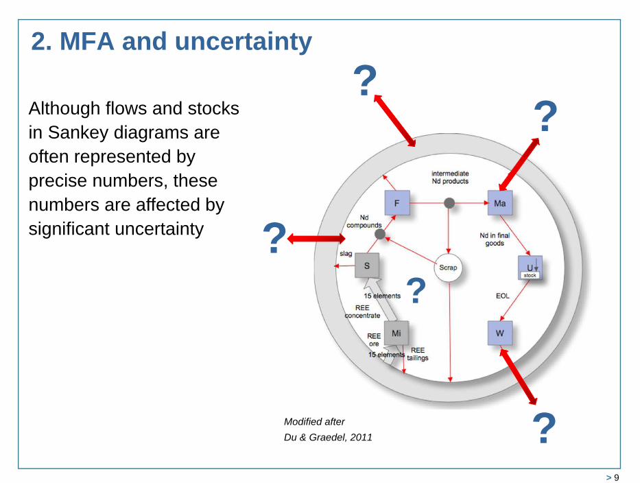
2. MFA and uncertainty

?

?

?

?

Modified afterDu & Graedel, 2011

?

Although flows and stocks in Sankey diagrams are often represented by precise numbers, these numbers are affected by significant uncertainty

> 10

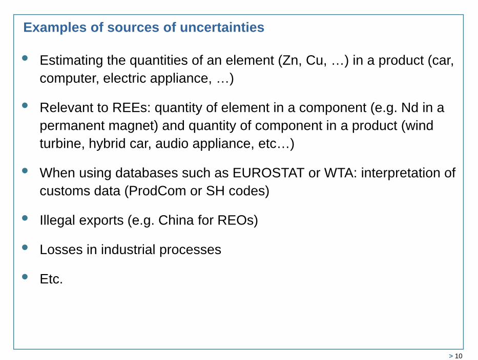
Examples of sources of uncertainties

• Estimating the quantities of an element (Zn, Cu, …) in a product (car, computer, electric appliance, …)

• Relevant to REEs: quantity of element in a component (e.g. Nd in a permanent magnet) and quantity of component in a product (wind turbine, hybrid car, audio appliance, etc…)

• When using databases such as EUROSTAT or WTA: interpretation of customs data (ProdCom or SH codes)

• Illegal exports (e.g. China for REOs)

• Losses in industrial processes

• Etc.

> 11

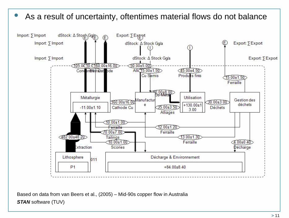
• As a result of uncertainty, oftentimes material flows do not balance

Based on data from van Beers et al., (2005) – Mid-90s copper flow in AustraliaSTAN software (TUV)

> 12

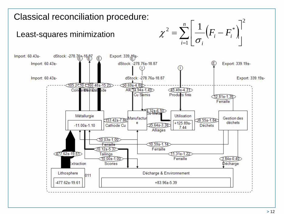
Classical reconciliation procedure:

Least-squares minimization 2

1

*2 1

n

iii

i

FF

> 13

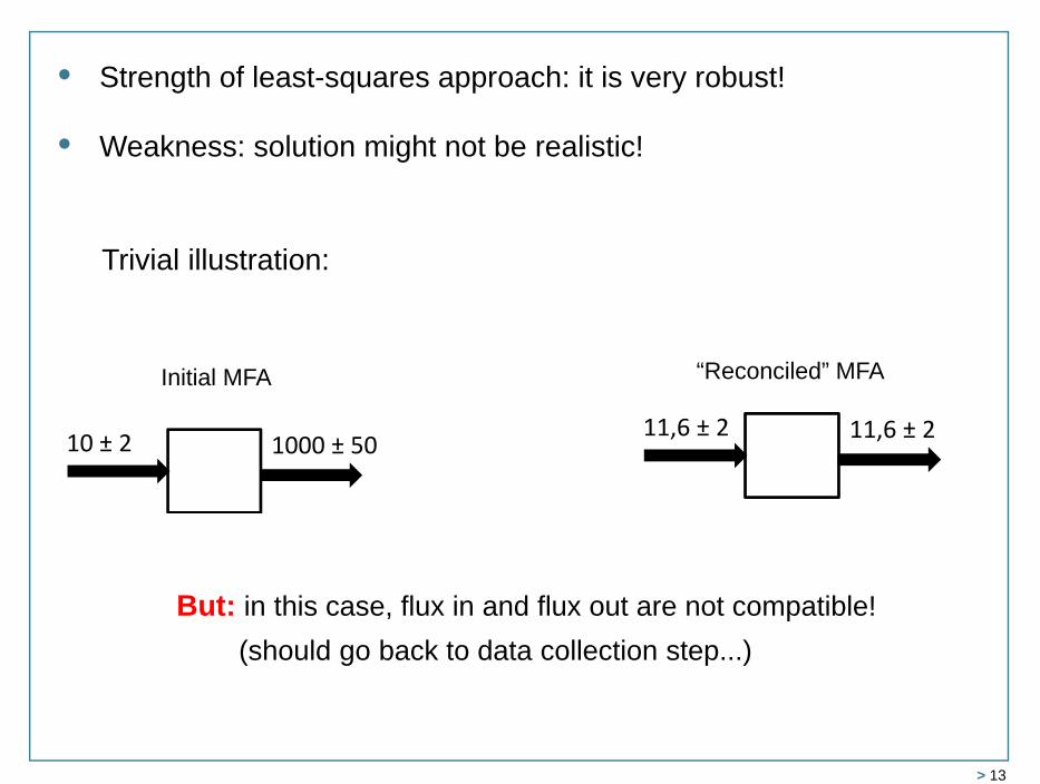
• Strength of least-squares approach: it is very robust!

• Weakness: solution might not be realistic!

Trivial illustration:

10 ± 2 1000 ± 5011,6 ± 2 11,6 ± 2

Initial MFA “Reconciled” MFA

But: in this case, flux in and flux out are not compatible! (should go back to data collection step...)

> 14

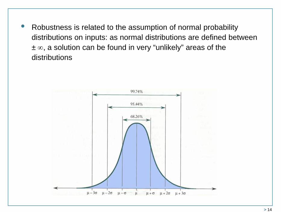
• Robustness is related to the assumption of normal probability distributions on inputs: as normal distributions are defined between ± , a solution can be found in very “unlikely” areas of the distributions

> 15

Message réel Message perçu

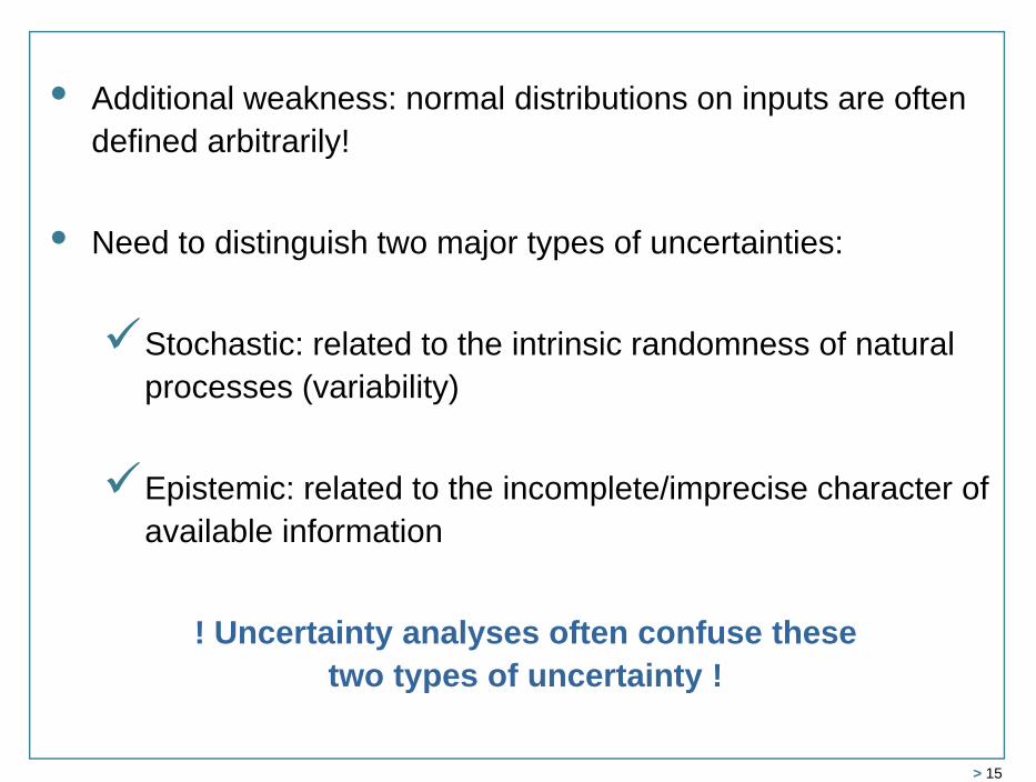
• Additional weakness: normal distributions on inputs are often defined arbitrarily!

• Need to distinguish two major types of uncertainties:

Stochastic: related to the intrinsic randomness of natural processes (variability)

Epistemic: related to the incomplete/imprecise character of available information

! Uncertainty analyses often confuse these two types of uncertainty !

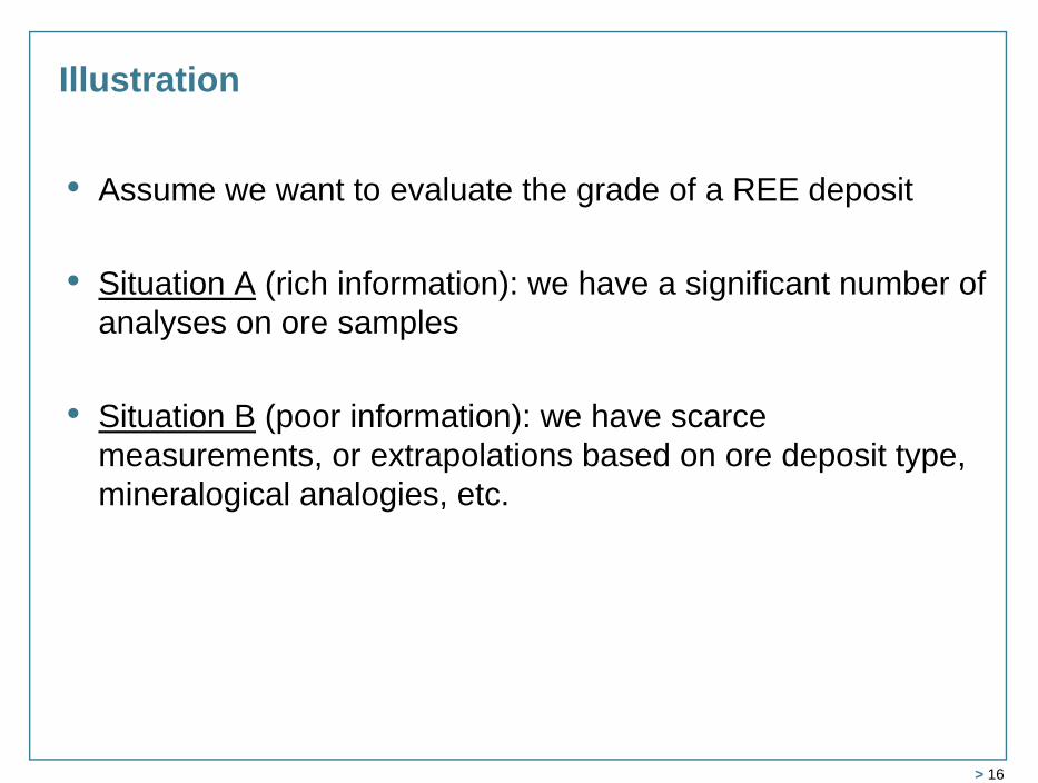
• Assume we want to evaluate the grade of a REE deposit

• Situation A (rich information): we have a significant number of analyses on ore samples

• Situation B (poor information): we have scarce measurements, or extrapolations based on ore deposit type, mineralogical analogies, etc.

Illustration

> 16

0

0,1

0,2

0,3

0,4

0,5

0,6

0,7

0,8

0,9

1

2 4 6 8 10 12 14 16

Fréq

uenc

es r

elat

ives

cum

ulée

s

Teneur en oxydes de terres rares (%)

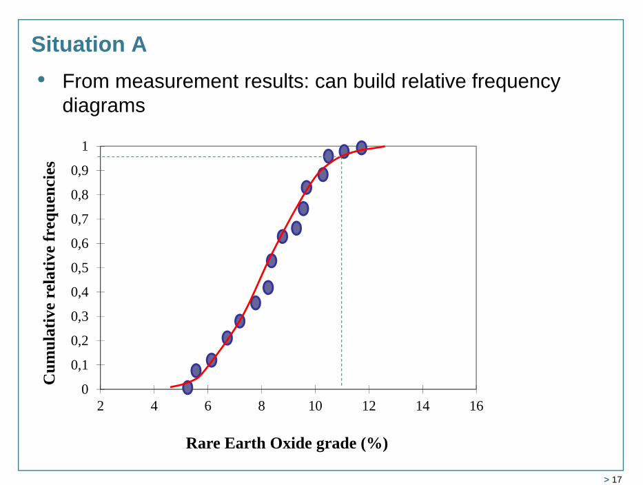
• From measurement results: can build relative frequency diagrams

Situation A

Rare Earth Oxide grade (%)

Cum

ulat

ive

rela

tive

freq

uenc

ies

> 17

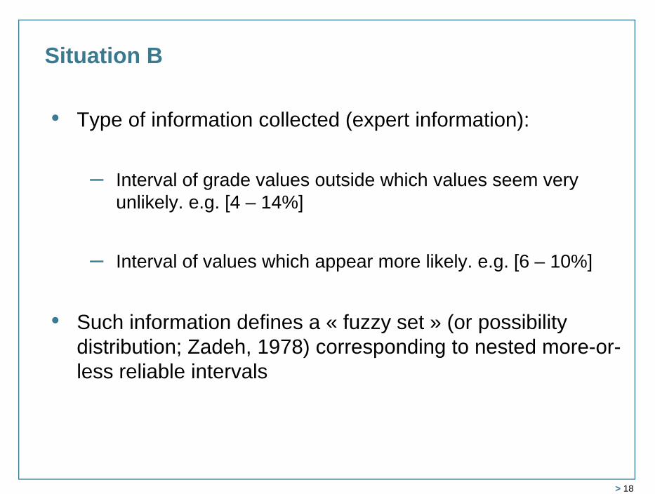
• Type of information collected (expert information):

– Interval of grade values outside which values seem very unlikely. e.g. [4 – 14%]

– Interval of values which appear more likely. e.g. [6 – 10%]

• Such information defines a « fuzzy set » (or possibility distribution; Zadeh, 1978) corresponding to nested more-or-less reliable intervals

Situation B

> 18

0

0,2

0,4

0,6

0,8

1

2 4 6 8 10 12 14 16

Poss

ibili

té

Teneur en oxydes de terres raresRare Earth Oxide grade (%)

Poss

ibili

ty

> 19

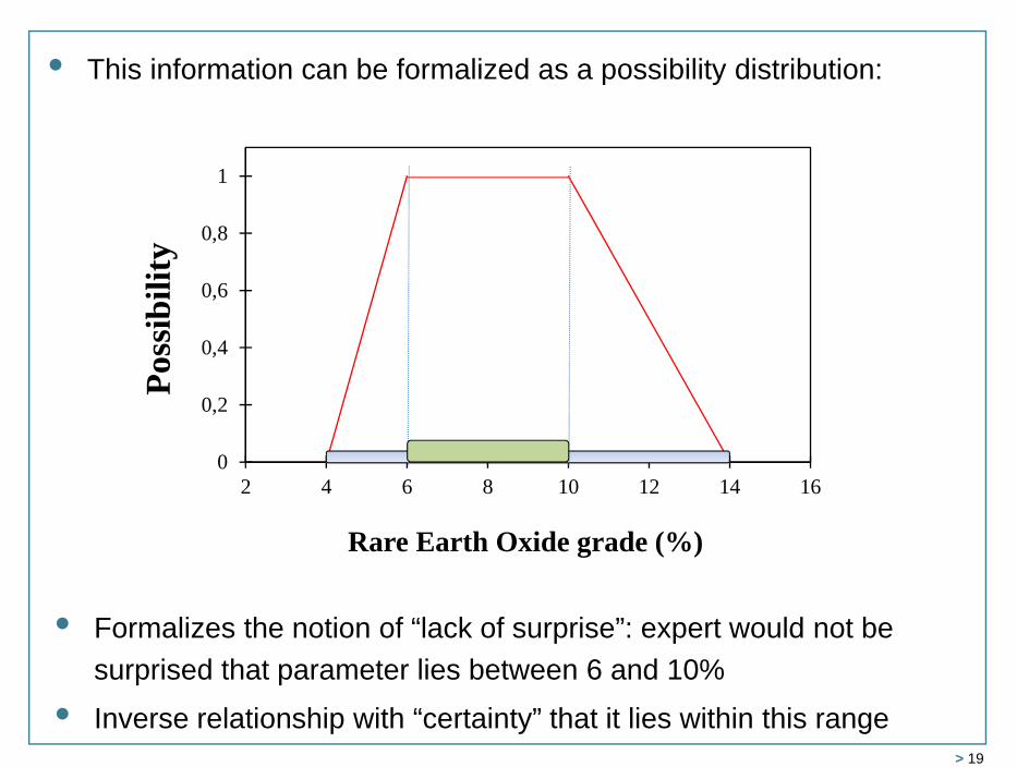
• This information can be formalized as a possibility distribution:

• Formalizes the notion of “lack of surprise”: expert would not be surprised that parameter lies between 6 and 10%

• Inverse relationship with “certainty” that it lies within this range

00,10,20,30,40,50,60,70,80,9

1

2 4 6 8 10 12 14 16

Prob

abili

té P

(x <

X)

Teneur en oxydes de terres rares (%)

limite haute de probabilité

limite basse 

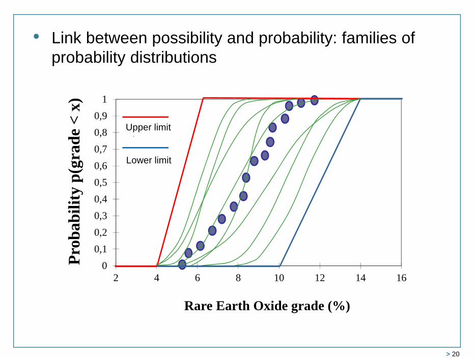
• Link between possibility and probability: families of probability distributions

Rare Earth Oxide grade (%)

Prob

abili

typ(

grad

e <

x)

Lower limit

Upper limit

> 20

> 21

• We have developed methods, in the 90s, to jointly address probabilistic and possibilistic information in engineering problems (risk analysis)

• These methods are being applied by an increasing number of researchers in various areas:

– Groundwater contamination (Zhang et al., 2009, Qin et al., 2009, Li et al., 2007)

– Soil erosion (Guneralp et al., 2007)– Ageing of water distribution systems (Tesfamariam et al., 2006)– Exposure to emissions from waste incinerators (Kumar et al., 2009)– Radionuclide migration in the envronment (Baccou et al., 2008)– Health risks (Kentel et Aral, 2005)– Greenhouse gas sequestration (Bellenfant et al., 2008)– Impact of waves on the shoreline (Koç, 2009)– …

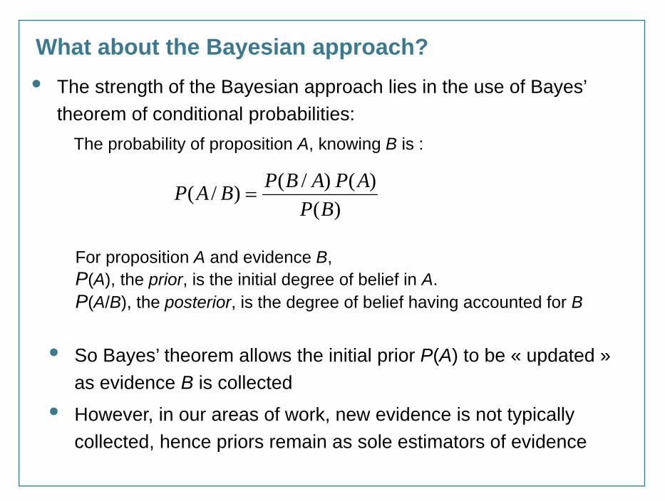
• The strength of the Bayesian approach lies in the use of Bayes’ theorem of conditional probabilities:

The probability of proposition A, knowing B is :

What about the Bayesian approach?

)()( )/()/(

BPAPABPBAP

For proposition A and evidence B,P(A), the prior, is the initial degree of belief in A.P(A/B), the posterior, is the degree of belief having accounted for B

• So Bayes’ theorem allows the initial prior P(A) to be « updated » as evidence B is collected

• However, in our areas of work, new evidence is not typically collected, hence priors remain as sole estimators of evidence

0.00 0.05 0.10 0.15

BCF

0.00

0.20

0.40

0.60

0.80

1.00

Cum

ulat

ive

prob

abili

ty

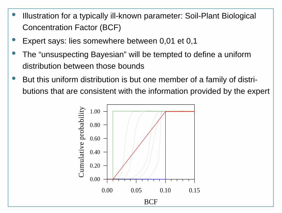
• Illustration for a typically ill-known parameter: Soil-Plant Biological Concentration Factor (BCF)

• Expert says: lies somewhere between 0,01 et 0,1

• The “unsuspecting Bayesian” will be tempted to define a uniform distribution between those bounds

• But this uniform distribution is but one member of a family of distri-butions that are consistent with the information provided by the expert

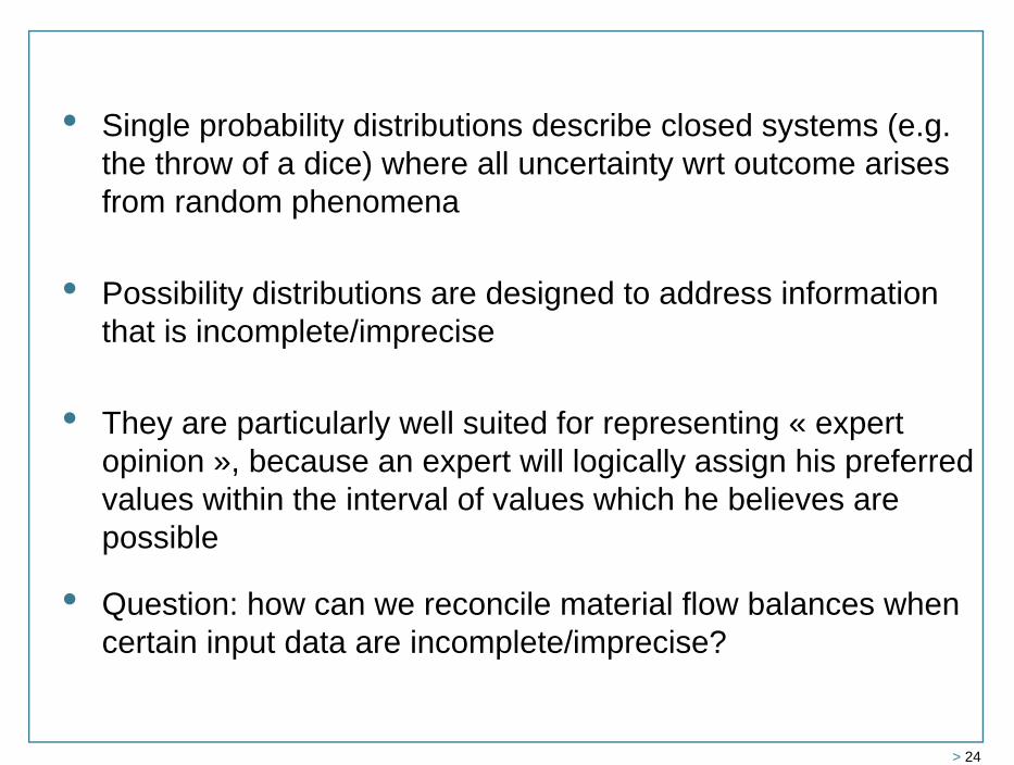
• Single probability distributions describe closed systems (e.g. the throw of a dice) where all uncertainty wrt outcome arises from random phenomena

• Possibility distributions are designed to address information that is incomplete/imprecise

• They are particularly well suited for representing « expert opinion », because an expert will logically assign his preferred values within the interval of values which he believes are possible

• Question: how can we reconcile material flow balances when certain input data are incomplete/imprecise?

> 24

> 25

3. Proposed alternative approach

> 26

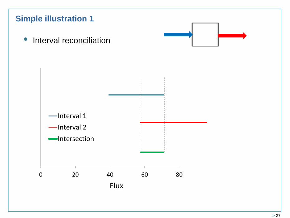
Data reconciliation under fuzzy constraints

• Principle: minimize the maximum deviation between information on each quantity, rather than minimize an average squared error

• Analogous to looking for maximum consistency between intervals at various levels of likelihood

0 20 40 60 80

Flux

Interval 1Interval 2Intersection

> 27

Simple illustration 1

• Interval reconciliation

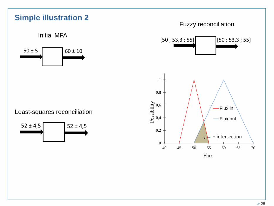
> 28

50 ± 5 60 ± 10

52 ± 4,5 52 ± 4,5

[50 ; 53,3 ; 55] [50 ; 53,3 ; 55]

intersection0

0,2

0,4

0,6

0,8

1

40 45 50 55 60 65 70Po

ssib

ility

Flux

Flux in

Flux out

Initial MFA

Least-squares reconciliation

Fuzzy reconciliationSimple illustration 2

> 29

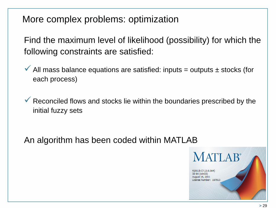
Find the maximum level of likelihood (possibility) for which the following constraints are satisfied:

All mass balance equations are satisfied: inputs = outputs ± stocks (for each process)

Reconciled flows and stocks lie within the boundaries prescribed by the initial fuzzy sets

An algorithm has been coded within MATLAB

More complex problems: optimization

> 30

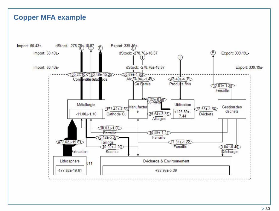
Copper MFA example

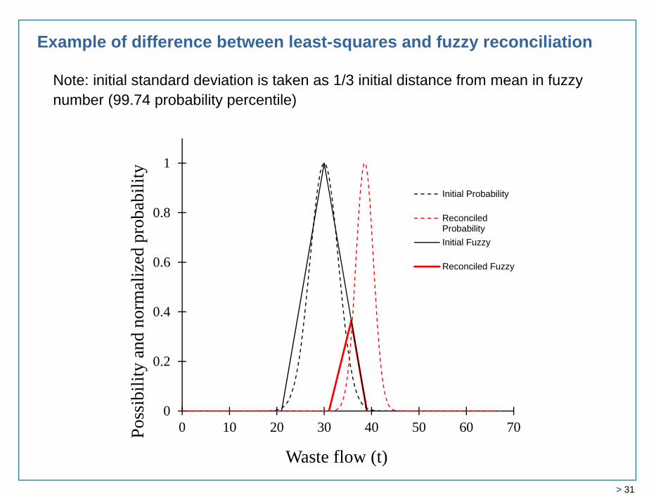
> 31

0

0.2

0.4

0.6

0.8

1

0 10 20 30 40 50 60 70Poss

ibili

ty a

nd n

orm

aliz

ed p

roba

bilit

y

Waste flow (t)

Initial Probability

ReconciledProbabilityInitial Fuzzy

Reconciled Fuzzy

Example of difference between least-squares and fuzzy reconciliation

Note: initial standard deviation is taken as 1/3 initial distance from mean in fuzzy number (99.74 probability percentile)

> 32

4. Concluding comments• MFAs and Sankey diagrams provide a systemic view of material

flows and stocks in the economy

• While data-mining is the crucial step, data are typically fraught with uncertainties that are often epistemic (knowledge gaps) rather than stochastic (randomness)

• The proposed approach wrt uncertainty representation aims at formalizing expert opinion in a more consistent manner than with a single normal probability distribution

• The proposed method avoids “force-fitting” unrealistic solutions as can sometimes be the case with the least-squares method

• It is a possible alternative to the least-squares method in situations where information is incomplete/imprecise

> 33

Thank you for your attention

Nd, Pr, Dy, Tb

Y, Er… ?

Y, Eu, La, Ce, Tb