Embed Size (px)
Citation preview

Uncertain knowledge and
Reasoning
Artificial Intelligence
Slides are taken from Svetlana Lazebnik (UIUC)

Where are we?
• Now leaving: sequential, deterministic reasoning
• Entering: probabilistic reasoning and machine learning

Probability:
Review of main concepts

Making decisions under uncertainty
• Let action At = leave for airport t minutes before flight
– Will At succeed, i.e., get me to the airport in time for the flight?
• Problems:
• Partial observability (road state, other drivers' plans, etc.)
• Noisy sensors (traffic reports)
• Uncertainty in action outcomes (flat tire, etc.)
• Complexity of modeling and predicting traffic
• Hence a non-probabilistic approach either
• Risks falsehood: “A25 will get me there on time,” or
• Leads to conclusions that are too weak for decision making:
• A25 will get me there on time if there's no accident on the bridge and it doesn't rain
and my tires remain intact, etc., etc.
• A1440 will get me there on time but I’ll have to stay overnight in the airport

Making decisions under uncertainty
• Suppose the agent believes the following:
P(A25 gets me there on time) = 0.04
P(A90 gets me there on time) = 0.70
P(A120 gets me there on time) = 0.95
P(A1440 gets me there on time) = 0.9999
• Which action should the agent choose?
– Depends on preferences for missing flight vs. time spent waiting
– Encapsulated by a utility function
• The agent should choose the action that maximizes the expected
utility:
P(At succeeds) * U(At succeeds) + P(At fails) * U(At fails)

Making decisions under uncertainty
• More generally: the expected utility of an action is defined as:
EU(a) = Σoutcomes of a P(outcome|a) U(outcome)
• Utility theory is used to represent and infer preferences
• Decision theory = probability theory + utility theory

Monty Hall problem
• You’re a contestant on a game show. You see three closed doors, and behind one of them is a prize. You choose one door, and the host opens one of the other doors and reveals that there is no prize behind it. Then he offers you a chance to switch to the remaining door. Should you take it?
http://en.wikipedia.org/wiki/Monty_Hall_problem

Monty Hall problem
• With probability 1/3, you picked the correct door, and with probability 2/3, picked the wrong door. If you picked the correct door and then you switch, you lose. If you picked the wrong door and then you switch, you win the prize.
• Expected utility of switching:
EU(Switch) = (1/3) * 0 + (2/3) * Prize
• Expected utility of not switching:
EU(Not switch) = (1/3) * Prize + (2/3) * 0

Random variables
• We describe the (uncertain) state of the world using random variables Denoted by capital letters
– R: Is it raining?
– W: What’s the weather?
– D: What is the outcome of rolling two dice?
– S: What is the speed of my car (in MPH)?
• Just like variables in CSPs, random variables take on values in a domain Domain values must be mutually exclusive and exhaustive
– R in {True, False}
– W in {Sunny, Cloudy, Rainy, Snow}
– D in {(1,1), (1,2), … (6,6)}
– S in [0, 200]

Events
• Probabilistic statements are defined over events, or sets of world states “It is raining”
“The weather is either cloudy or snowy”
“The sum of the two dice rolls is 11”
“My car is going between 30 and 50 miles per hour”
• Events are described using propositions about random variables: R = True
W = “Cloudy” W = “Snowy”
D {(5,6), (6,5)}
30 S 50
• Notation: P(A) is the probability of the set of world states in which proposition A holds

Kolmogorov’s axioms of probability
• For any propositions (events) A, B
0 ≤ P(A) ≤ 1
P(True) = 1 and P(False) = 0
P(A B) = P(A) + P(B) – P(A B)– Subtraction accounts for double-counting
• Based on these axioms, what is P(¬A)?
• These axioms are sufficient to completely specify probability theory for discrete random variables• For continuous variables, need density functions

Atomic events
• Atomic event: a complete specification of the state of the world, or a complete assignment of domain values to all random variables
– Atomic events are mutually exclusive and exhaustive
• E.g., if the world consists of only two Boolean variables Cavity and Toothache, then there are four distinct atomic events:
Cavity = false Toothache = falseCavity = false Toothache = trueCavity = true Toothache = falseCavity = true Toothache = true

Joint probability distributions
• A joint distribution is an assignment of probabilities to every possible atomic event
– Why does it follow from the axioms of probability that the probabilities of all possible atomic events must sum to 1?
Atomic event P
Cavity = false Toothache = false 0.8
Cavity = false Toothache = true 0.1
Cavity = true Toothache = false 0.05
Cavity = true Toothache = true 0.05

Joint probability distributions
• A joint distribution is an assignment of probabilities to every possible atomic event
• Suppose we have a joint distribution of n random variables with domain sizes d– What is the size of the probability table?
– Impossible to write out completely for all but the smallest distributions

Notation
• P(X1 = x1, X2 = x2, …, Xn = xn) refers to a single entry
(atomic event) in the joint probability distribution table
– Shorthand: P(x1, x2, …, xn)
• P(X1, X2, …, Xn) refers to the entire joint probability
distribution table
• P(A) can also refer to the probability of an event
– E.g., X1 = x1 is an event

Marginal probability distributions
• From the joint distribution P(X,Y) we can find the marginal distributions P(X) and P(Y)
P(Cavity, Toothache)
Cavity = false Toothache = false 0.8
Cavity = false Toothache = true 0.1
Cavity = true Toothache = false 0.05
Cavity = true Toothache = true 0.05
P(Cavity)
Cavity = false ?
Cavity = true ?
P(Toothache)
Toothache = false ?
Toochache = true ?

Marginal probability distributions
• From the joint distribution P(X,Y) we can find the marginal distributions P(X) and P(Y)
• To find P(X = x), sum the probabilities of all atomic events where X = x:
• This is called marginalization (we are marginalizing out all the variables except X)
n
i
in
n
yxPyxyxP
yYxXyYxXPxXP
1
1
1
),(),(),(
)()()(

Conditional probability
• Probability of cavity given toothache: P(Cavity = true | Toothache = true)
• For any two events A and B,
)(
),(
)(
)()|(
BP
BAP
BP
BAPBAP
P(A) P(B)
P(A B)

Conditional probability
• What is P(Cavity = true | Toothache = false)?0.05 / 0.85 = 0.059
• What is P(Cavity = false | Toothache = true)?0.1 / 0.15 = 0.667
P(Cavity, Toothache)
Cavity = false Toothache = false 0.8
Cavity = false Toothache = true 0.1
Cavity = true Toothache = false 0.05
Cavity = true Toothache = true 0.05
P(Cavity)
Cavity = false 0.9
Cavity = true 0.1
P(Toothache)
Toothache = false 0.85
Toothache = true 0.15

Conditional distributions
• A conditional distribution is a distribution over the values of one variable given fixed values of other variables
P(Cavity, Toothache)
Cavity = false Toothache = false 0.8
Cavity = false Toothache = true 0.1
Cavity = true Toothache = false 0.05
Cavity = true Toothache = true 0.05
P(Cavity | Toothache = true)
Cavity = false 0.667
Cavity = true 0.333
P(Cavity|Toothache = false)
Cavity = false 0.941
Cavity = true 0.059
P(Toothache | Cavity = true)
Toothache= false 0.5
Toothache = true 0.5
P(Toothache | Cavity = false)
Toothache= false 0.889
Toothache = true 0.111

Normalization trick
• To get the whole conditional distribution P(X | Y = y) at once, select all entries in the joint distribution table matching Y = y and renormalize them to sum to one
P(Cavity, Toothache)
Cavity = false Toothache = false 0.8
Cavity = false Toothache = true 0.1
Cavity = true Toothache = false 0.05
Cavity = true Toothache = true 0.05
Toothache, Cavity = false
Toothache= false 0.8
Toothache = true 0.1
P(Toothache | Cavity = false)
Toothache= false 0.889
Toothache = true 0.111
Select
Renormalize

Normalization trick
• To get the whole conditional distribution P(X | Y = y) at once, select all entries in the joint distribution table matching Y = y and renormalize them to sum to one
• Why does it work?
)(
),(
),(
),(
yP
yxP
yxP
yxP
x
by marginalization

Product rule
• Definition of conditional probability:
• Sometimes we have the conditional probability and want to obtain the joint:
)(
),()|(
BP
BAPBAP
)()|()()|(),( APABPBPBAPBAP

Chain rule
• Product rule:
• Chain rule:
)()|()()|(),( APABPBPBAPBAP
n
i
ii
nnn
AAAP
AAAPAAAPAAPAPAAP
1
11
112131211
),,|(
),,|(),|()|()(),,(

Independence
• Two events A and B are independent if and only if P(A B) = P(A, B) = P(A) P(B)
– In other words, P(A | B) = P(A) and P(B | A) = P(B)
– This is an important simplifying assumption for modeling, e.g., Toothache and Weather can be assumed to be independent
• Are two mutually exclusive events independent?
– No, but for mutually exclusive events we have P(A B) = P(A) + P(B)

Independence
• Two events A and B are independent if and only if P(A B) = P(A, B) = P(A) P(B)
– In other words, P(A | B) = P(A) and P(B | A) = P(B)
– This is an important simplifying assumption for modeling, e.g., Toothache and Weather can be assumed to be independent
• Conditional independence: A and B are conditionally independent given C iff P(A B | C) = P(A | C) P(B | C)
– Equivalently:P(A | B, C) = P(A | C) or P(B | A, C) = P(B | C)

Conditional independence: Example
• Toothache: boolean variable indicating whether the patient has a toothache
• Cavity: boolean variable indicating whether the patient has a cavity
• Catch: whether the dentist’s probe catches in the cavity
• If the patient has a cavity, the probability that the probe catches in it doesn't depend on whether he/she has a toothache
P(Catch | Toothache, Cavity) = P(Catch | Cavity)
• Therefore, Catch is conditionally independent of Toothache given Cavity
• Likewise, Toothache is conditionally independent of Catch given Cavity
P(Toothache | Catch, Cavity) = P(Toothache | Cavity)
• Equivalent statement:
P(Toothache, Catch | Cavity) = P(Toothache | Cavity) P(Catch | Cavity)

Conditional independence: Example
• How many numbers do we need to represent the joint probability table P(Toothache, Cavity, Catch)?
23 – 1 = 7 independent entries
• Write out the joint distribution using chain rule:
P(Toothache, Catch, Cavity)
= P(Cavity) P(Catch | Cavity) P(Toothache | Catch, Cavity)
= P(Cavity) P(Catch | Cavity) P(Toothache | Cavity)
• How many numbers do we need to represent these distributions?
1 + 2 + 2 = 5 independent numbers
• In most cases, the use of conditional independence reduces the size of the representation of the joint distribution from exponential in n to linear in n

Bayes Rule
• The product rule gives us two ways to factor
a joint probability:
• Therefore,
• Why is this useful?
– Can update our beliefs about A based on evidence B
• P(A) is the prior and P(A|B) is the posterior
– Key tool for probabilistic inference: can get diagnostic probability from
causal probability
• E.g., P(Cavity = true | Toothache = true) from
P(Toothache = true | Cavity = true)
)()|()()|(),( APABPBPBAPBAP
)(
)()|()|(
BP
APABPBAP
Rev. Thomas Bayes
(1702-1761)

Bayes Rule example
• Marie is getting married tomorrow, at an outdoor ceremony in the desert. In recent years, it has rained only 5 days each year (5/365 = 0.014). Unfortunately, the weatherman has predicted rain for tomorrow. When it actually rains, the weatherman correctly forecasts rain 90% of the time. When it doesn't rain, he incorrectly forecasts rain 10% of the time. What is the probability that it will rain on Marie's wedding?
P(rain | predict) =P(predict | rain)P(rain)
P(predict)
=P(predict | rain)P(rain)
P(predict | rain)P(rain)+P(predict | Ørain)P(Ørain)

Law of total probability
P(X = x) = P(X = x,Y = yi )i=1
n
å
= P(X = x |Y = yi )P(i=1
n
å Y = yi )

Bayes Rule example
• Marie is getting married tomorrow, at an outdoor ceremony in the desert. In recent years, it has rained only 5 days each year (5/365 = 0.014). Unfortunately, the weatherman has predicted rain for tomorrow. When it actually rains, the weatherman correctly forecasts rain 90% of the time. When it doesn't rain, he incorrectly forecasts rain 10% of the time. What is the probability that it will rain on Marie's wedding?
P(rain | predict) =P(predict | rain)P(rain)
P(predict)
111.00986.00126.0
0126.0
986.01.0014.09.0
014.09.0
=P(predict | rain)P(rain)
P(predict | rain)P(rain)+P(predict | Ørain)P(Ørain)

Bayes rule: Example
• 1% of women at age forty who participate in routine screening have breast cancer. 80% of women with breast cancer will get positive mammographies. 9.6% of women without breast cancer will also get positive mammographies. A woman in this age group had a positive mammography in a routine screening. What is the probability that she actually has breast cancer?
P(cancer | positive) =P(positive | cancer)P(cancer)
P(positive)
0776.0095.0008.0
008.0
99.0096.001.08.0
01.08.0
=P(positive | cancer)P(cancer)
P(positive | cancer)P(cancer)+P(positive | Øcancer)P(Øcancer)

Probabilistic inference
• Suppose the agent has to make a decision about the value
of an unobserved query variable X given some observed
evidence variable(s) E = e
– Partially observable, stochastic, episodic environment
– Examples: X = {spam, not spam}, e = email message
X = {zebra, giraffe, hippo}, e = image features

MAP decision
• Value x of X that has the highest posterior probability given the evidence E = e:
• Maximum likelihood (ML) decision:
x̂ = argmaxx P(e | x)
)()|()|( xPxePexP
likelihood priorposterior
x̂ = argmaxx P(X = x |E = e) =P(E = e | X = x)P(X = x)
P(E = e)
)()|(maxarg xXPxXeEPx

Naïve Bayes model
• Suppose we have many different types of observations (symptoms, features) E1, …, En that we want to use to obtain evidence about an underlying hypothesis X
• MAP decision:
• We can make the simplifying assumption that the different features are conditionally independent given the hypothesis:
– If each feature can take on d values, what is the complexity of storing the resulting distributions?
P(E1 = e1, ... , En = en | X = x) =
P(X = x |E1 = e1, ... , En = en )
µP(X = x)P(E1 = e1, ... , En = en | X = x)
P(Ei = ei | X = x)i=1
n
Õ

Naïve Bayes model
• Posterior:
• MAP decision:
P(X = x |E1 = e1, ... , En = en )
µP(X = x)P(E1 = e1, ... , En = en | X = x)
= P(X = x) P(Ei = ei | X = x)i=1
n
Õ
likelihoodpriorposterior
x̂ = argmaxx P(x | e)µP(x) P(ei | x)i=1
n
Õ

Case study: Text document classification
• MAP decision: assign a document to the class with the highest posterior P(class | document)
• Example: spam classification– Classify a message as spam if P(spam | message) > P(¬spam | message)

Case study: Text document classification
• MAP decision: assign a document to the class with the highest posterior P(class | document)
• We have P(class | document) P(document | class)P(class)
• To enable classification, we need to be able to estimate the likelihoodsP(document | class) for all classes andpriors P(class)

Naïve Bayes Representation
• Goal: estimate likelihoods P(document | class) and priors P(class)
• Likelihood: bag of words representation– The document is a sequence of words (w1, …, wn)
– The order of the words in the document is not important
– Each word is conditionally independent of the others given document class
P(document | class) = P(w1, ... ,wn | class) = P(wi | class)i=1
n
Õ

Naïve Bayes Representation
• Goal: estimate likelihoods P(document | class) and P(class)
• Likelihood: bag of words representation– The document is a sequence of words (w1, … , wn)
– The order of the words in the document is not important
– Each word is conditionally independent of the others given document class
– Thus, the problem is reduced to estimating marginal likelihoods of individual words P(wi | class)
P(document | class) = P(w1, ... ,wn | class) = P(wi | class)i=1
n
Õ

Parameter estimation
• Model parameters: feature likelihoods P(word | class) and priorsP(class)
– How do we obtain the values of these parameters?
spam: 0.33
¬spam: 0.67
P(word | ¬spam)P(word | spam)prior

Parameter estimation
• Model parameters: feature likelihoods P(word | class) and priorsP(class)
– How do we obtain the values of these parameters?
– Need training set of labeled samples from both classes
– This is the maximum likelihood (ML) estimate, or estimate that maximizes the likelihood of the training data:
P(word | class) =# of occurrences of this word in docs from this class
total # of words in docs from this class
D
d
n
i
idid
d
classwP1 1
,, )|(
d: index of training document, i: index of a word

Parameter estimation
• Parameter estimate:
• Parameter smoothing: dealing with words that were never seen or seen too few times
– Laplacian smoothing: pretend you have seen every vocabulary word one more time than you actually did
P(word | class) =# of occurrences of this word in docs from this class + 1
total # of words in docs from this class + V
(V: total number of unique words)
P(word | class) =# of occurrences of this word in docs from this class
total # of words in docs from this class

Summary: Naïve Bayes for Document Classification
• Assign the document to the class with the highest posterior
• Model parameters:
P(class | document)µP(class) P(wi | class)i=1
n
Õ
P(class1)
…
P(classK)
P(w1 | class1)
P(w2 | class1)
…
P(wn | class1)
Likelihood
of class 1prior
P(w1 | classK)
P(w2 | classK)
…
P(wn | classK)
Likelihood
of class K
…

Summary: Naïve Bayes for Document Classification
• Assign the document to the class with the highest posterior
• Note: by convention, one typically works with logs of probabilities instead:
– Can help to avoid underflow
P(class | document)µP(class) P(wi | class)i=1
n
Õ
L(class | document) = logP(class)+ logP(wi | class)i=1
n
å

Bayesian networks
• More commonly called graphical models
• A way to depict conditional independence relationships between random variables
• A compact specification of full joint distributions

Bayesian networks: Structure
• Nodes: random variables
• Arcs: interactions– An arrow from one variable to another indicates
direct influence
– Must form a directed, acyclic graph

Example: N independent coin flips
• Complete independence: no interactions
X1 X2 Xn…

Example: Naïve Bayes document model
• Random variables:– X: document class
– W1, …, Wn: words in the document
W1 W2 Wn…
X

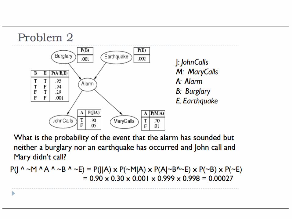
Example: Burglar Alarm
• I have a burglar alarm that is sometimes set off by minor
earthquakes. My two neighbors, John and Mary, promised
to call me at work if they hear the alarm
• Example inference tasks
– Suppose Mary calls and John doesn’t call. What is the probability
of a burglary?
– Suppose there is a burglary and no earthquake. What is the
probability of John calling?
– Suppose the alarm went off. What is the probability of burglary?
– …

Example: Burglar Alarm
• I have a burglar alarm that is sometimes set off by minor
earthquakes. My two neighbors, John and Mary, promised
to call me at work if they hear the alarm
• What are the random variables?
– Burglary, Earthquake, Alarm, John, Mary
• What are the direct influence relationships?
– A burglar can set the alarm off
– An earthquake can set the alarm off
– The alarm can cause Mary to call
– The alarm can cause John to call

Example: Burglar Alarm

Conditional independence relationships
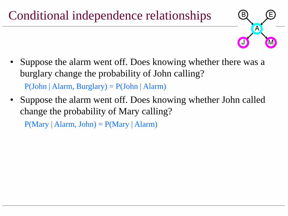
• Suppose the alarm went off. Does knowing whether there was a
burglary change the probability of John calling?
P(John | Alarm, Burglary) = P(John | Alarm)
Conditional independence relationships
• Suppose the alarm went off. Does knowing whether there was a
burglary change the probability of John calling?
P(John | Alarm, Burglary) = P(John | Alarm)
• Suppose the alarm went off. Does knowing whether John called
change the probability of Mary calling?
P(Mary | Alarm, John) = P(Mary | Alarm)
• Suppose the alarm went off. Does knowing whether there was an
earthquake change the probability of burglary?
P(Burglary | Alarm, Earthquake) != P(Burglary | Alarm)
• Suppose there was a burglary. Does knowing whether John called
change the probability that the alarm went off?
P(Alarm | Burglary, John) != P(Alarm | Burglary)

Conditional independence relationships
• John and Mary are conditionally independent of Burglary and Earthquake given
Alarm
– Children are conditionally independent of ancestors given parents

Conditional independence relationships
• John and Mary are conditionally independent of Burglary and Earthquake given
Alarm
– Children are conditionally independent of ancestors given parents
• John and Mary are conditionally independent of each other given Alarm
– Siblings are conditionally independent of each other given parents
• Burglary and Earthquake are not conditionally independent of each other given
Alarm
– Parents are not conditionally independent given children

Conditional independence relationships
• John and Mary are conditionally independent of Burglary and Earthquake given Alarm
– Children are conditionally independent of ancestors given parents
• John and Mary are conditionally independent of each other given Alarm
– Siblings are conditionally independent of each other given parents
• Burglary and Earthquake are not conditionally independent of each other given Alarm
– Parents are not conditionally independent given children
• Alarm is not conditionally independent of John and Mary given Burglary and Earthquake
– Nodes are not conditionally independent of children given parents
• General rule: each node is conditionally independent of its non-descendants given its parents

Conditional independence and the joint distribution
• General rule: each node is conditionally independent of its
non-descendants given its parents
• Suppose the nodes X1, …, Xn are sorted in topological
order (parents before children)
• To get the joint distribution P(X1, …, Xn),
use chain rule:
n
i
iin XXXPXXP1
111 ,,|),,(
n
i
ii XParentsXP1
)(|
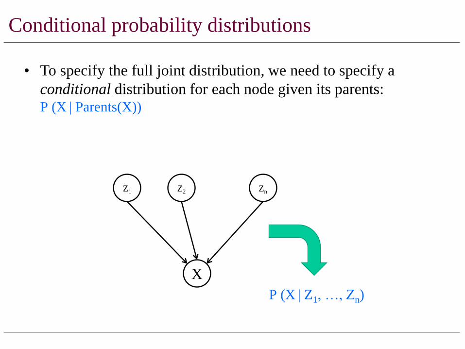
Conditional probability distributions
• To specify the full joint distribution, we need to specify a
conditional distribution for each node given its parents: P (X | Parents(X))
Z1 Z2 Zn
X
…
P (X | Z1, …, Zn)

Example: Burglar Alarm
The conditional
probability tables are
the model parameters

The joint probability distribution
• For example, P(j, m, a, b, e)
= P(b) P(e) P(a | b, e) P(j | a) P(m | a)
n
i
iin XParentsXPXXP1
1 )(|),,(

Bayes Nets

Conditional independence
• General rule: X is conditionally independent of every non-descendant node given its parents
• Example: causal chain
• Are X and Z independent?
• Is Z independent of X given Y?

Compactness
• Suppose we have a Boolean variable Xi with k Boolean parents. How many rows does its conditional probability table have?
– 2k rows for all the combinations of parent values
– Each row requires one number for P(Xi = true | parent values)
• If each variable has no more than k parents, how many numbers does the complete network require?
– O(n · 2k) numbers – vs. O(2n) for the full joint distribution
• How many nodes for the burglary network? 1 + 1 + 4 + 2 + 2 = 10 numbers (vs. 25-1 = 31)

Conditional independence
• Common cause
• Are X and Z independent?
– No
• Are they conditionally independent given Y?
– Yes
• Common effect
• Are X and Z independent?
– Yes
• Are they conditionally independent given Y?
– No

Constructing Bayesian networks
1. Choose an ordering of variables X1, … , Xn
2. For i = 1 to n
– add Xi to the network
– select parents from X1, … ,Xi-1 such thatP(Xi | Parents(Xi)) = P(Xi | X1, ... Xi-1)

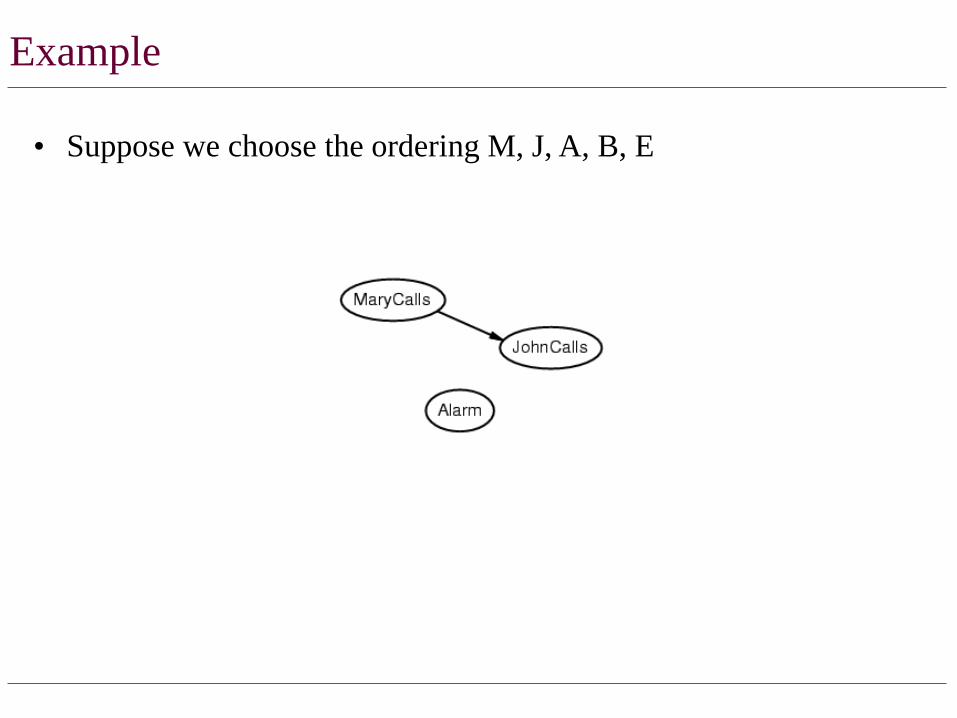
• Suppose we choose the ordering M, J, A, B, E
Example

• Suppose we choose the ordering M, J, A, B, E
Example
• Suppose we choose the ordering M, J, A, B, E
Example

• Suppose we choose the ordering M, J, A, B, E
Example

• Suppose we choose the ordering M, J, A, B, E
Example

• Suppose we choose the ordering M, J, A, B, E
Example

• Suppose we choose the ordering M, J, A, B, E
Example

• Suppose we choose the ordering M, J, A, B, E
Example

Example contd.
• Deciding conditional independence is hard in noncausal directions
– The causal direction seems much more natural
• Network is less compact: 1 + 2 + 4 + 2 + 4 = 13 numbers needed (vs. 10 for the causal ordering)

A more realistic Bayes Network: Car diagnosis
• Initial observation: car won’t start
• Orange: “broken, so fix it” nodes
• Green: testable evidence
• Gray: “hidden variables” to ensure sparse structure, reduce parameteres

Car insurance

In research literature…
Causal Protein-Signaling Networks Derived from Multiparameter Single-Cell Data
Karen Sachs, Omar Perez, Dana Pe'er, Douglas A. Lauffenburger, and Garry P. Nolan
(22 April 2005) Science 308 (5721), 523.

In research literature…
Describing Visual Scenes Using Transformed Objects and Parts
E. Sudderth, A. Torralba, W. T. Freeman, and A. Willsky.
International Journal of Computer Vision, No. 1-3, May 2008, pp. 291-330.

In research literature…
Audiovisual Speech Recognition with Articulator Positions as Hidden Variables
Mark Hasegawa-Johnson, Karen Livescu, Partha Lal and Kate Saenko
International Congress on Phonetic Sciences 1719:299-302, 2007
audio video

In research literature…
Detecting interaction links in a collaborating group using manually annotated data
S. Mathur, M.S. Poole, F. Pena-Mora, M. Hasegawa-Johnson, N. Contractor
Social Networks 10.1016/j.socnet.2012.04.002

In research literature…
Detecting interaction links in a collaborating group using manually annotated data
S. Mathur, M.S. Poole, F. Pena-Mora, M. Hasegawa-Johnson, N. Contractor
Social Networks 10.1016/j.socnet.2012.04.002
• Speaking: Si=1 if #i
is speaking.
• Link: Lij=1 if #i is
listening to #j.
• Neighborhood:
Nij=1 if they are
near one another.
• Gaze: Gij=1 if #i is
looking at #j.
• Indirect: Iij=1 if #i
and #j are both
listening to the same
person.

Summary
• Bayesian networks provide a natural representation for (causally induced) conditional independence
• Topology + conditional probability tables
• Generally easy for domain experts to construct

Bayes network inference
A general scenario:
Query variables: X
Evidence (observed) variables and their values: E = e
Unobserved variables: Y
Inference problem: answer questions about the query
variables given the evidence variables

Bayes network inference
A general scenario:
Query variables: X
Evidence (observed) variables and their values: E = e
Unobserved variables: Y
Inference problem: answer questions about the query
variables given the evidence variables
Example: what is the
probability of a burglary
given that John and
Mary called?

Bayes network inference
A general scenario:
Query variables: X
Evidence (observed) variables and their values: E = e
Unobserved variables: Y
Inference problem: answer questions about the query
variables given the evidence variables
This can be done using the posterior distribution P(X | E = e)
The posterior can be derived from the full joint P(X, E, Y)
Since Bayesian networks can afford exponential savings in
representing joint distributions, can they afford similar
savings for inference?
y
yeXe
eXeEX ),,(
)(
),()|( P
P
PP

Full Joint distribution


Burglary example
• Query: P(b | j, m)
P(b | j,m) =P(b, j,m)
P( j,m)µ P(b,e,a, j,m)E=e,A=a
å
= P(b)P(e)P(a | b,e)P( j | a)P(m | a)E=e,A=a
å


Example


Another example
• Variables: Cloudy, Sprinkler, Rain, WetGrass

Another example
• Given that the grass is wet, what is the probability that it has rained?
P(r |w) =P(r,w)
P(w)µ P(c, s, r,w)C=c,S=s
å
= P(c)P(s | c)P(r | c)P(w | r, s)C=c,S=s
å
= P(c)P(r | c) P(w | r, s)S=s
åC=c
å P(s | c)
= P(c)P(r | c)P(w | r,c)C=c
å
= P(w | r) P(r | c)P(c)C=c
å
= P(w | r)P(r)

• What determines whether you will pass the exam?– A: Do you attend class?
– S: Do you study?
– Pr: Are you prepared for the exam?
– F: Is the grading fair?
– Pa: Do you get a passing grade on the exam?
A S
PrF
Pa
Another example
Source: UMBC CMSC 671, Tamara Berg

Another example
Source: UMBC CMSC 671, Tamara Berg
A S P(Pr|A,S)
T T 0.9
T F 0.5
F T 0.7
F F 0.1
A S
PrF
Pa
P(A=T) = 0.8P(S=T) = 0.6
P(F=T) = 0.9
Pr A F P(Pa|A,Pr,F)
T T T 0.9
T T F 0.6
T F T 0.2
T F F 0.1
F T T 0.4
F T F 0.2
F F T 0.1
F F F 0.2

Another example
Query: What is the probability
that a student attended class,
given that they passed the
exam?
Source: UMBC CMSC 671, Tamara Berg
A S
PrF
PaP(a | pa)µP(a, pa)
= P(a, s, f , pr, pa)S=s,F= f ,Pr=pr
å
= P(a)P(s)P( f )P(pr | a, s)P(pa | a, pr, f )S=s,F= f ,Pr=pr
å

Efficient inference
• Query: P(b | j, m)
• Can we compute this sum efficiently?
P(b | j,m) =P(b, j,m)
P( j,m)µ P(b,e,a, j,m)E=e,A=a
å
= P(b)P(e)P(a | b,e)P( j | a)P(m | a)E=e,A=a
å

Efficient inference
eE aA
amPajPebaPePbPmjbP )|()|(),|()()(),|(

Efficient inference
• Key idea: compute the results of
sub-expressions in a bottom-up way and cache them
for later use
– Form of dynamic programming
– Polynomial time and space complexity for polytrees:
networks at most one undirected path between any two
nodes