tuprints.ulb.tu-darmstadt.de · Unbalance and Resonance Elimination on General Rotors with Active Bearings Am Fachbereich Maschinenbau an der Technischen Universität Darmstadt zur

Unbalance and ResonanceElimination on General Rotorswith Active BearingsUnwucht- und Resonanzeliminierung allgemeiner Rotorenmit aktiven LagernZur Erlangung des akademischen Grades Doktor-Ingenieur (Dr.-Ing.)genehmigte Dissertation von Stefan Heindel aus Hanau

Please cite this document as:URL: http://tuprints.ulb.tu-darmstadt.de/6967

This document is provided by tuprints,E-Publishing-Service of the TU Darmstadthttp://[email protected]

This work is published under the following Creative Commons license:Attribution -– Non Commercial -– No Derivatives 4.0https://creativecommons.org/licenses/by-nc-nd/4.0/

Unbalance and Resonance Eliminationon General Rotors with Active Bearings

Am Fachbereich Maschinenbau

an der Technischen Universität Darmstadt

zur

Erlangung des Grades eines Doktor-Ingenieurs (Dr.-Ing.)

genehmigte

Dissertation

vorgelegt von

Dipl.-Ing. Stefan Heindel

aus Hanau

Berichterstatter: Prof. Dr.-Ing. Stephan RinderknechtMitberichterstatter: Prof. Dr.-Ing. Bernhard Schweizer

Tag der Einreichung: 23.1.2017

Tag der mündlichen Prüfung: 19.4.2017

Darmstadt 2017

D 17

VorwortDie hier vorliegende Arbeit entstand während meiner Zeit als Promotionsstu-dent am Institut für Mechatronische Systeme im Maschinenbau im Rahmendes DFG geförderten Graduiertenkollegs 1344. Ich bedanke mich bei HerrnProfessor Dr.-Ing. Stephan RINDERKNECHT, der mir als Institutsleiter die Pro-motion ermöglichte und mir großes Vertrauen bei der Gestaltung der Arbeitentgegenbrachte. Bedanken möchte ich mich ebenfalls bei Herrn Professor Dr.-Ing. Bernhard SCHWEIZER, der die Zweitkorrektur der Arbeit übernahm.

Ein ganz besonderer Dank geht an Herrn Professor Dr.-Ing. Peter Chris-tian MÜLLER, der durch umfangreiche postalische Korrespondenz ganz erheblichzum Gelingen dieser Arbeit beitrug. Teile des Stabilitätsbeweises und insbeson-dere der Nachweis asymptotischer Stabilität basieren auf seinen Ausführungen.Sein herausragendes Fachwissen, die wissenschaftliche Präzision seiner Pub-likationen und sein freundlicher Umgang haben mich tief beeindruckt.

Die Kolleginnen und Kollegen machten das IMS zu einem Ort, an dem fachlicheund private Themen immer offen und in freundschaftlicher Atmosphäre disku-tiert werden konnten. In guter Erinnerung bleibt mir auch unsere SekretärinFrau Ursula WILLNER, welche die kleinen und großen Probleme des wis-senschaftlichen Alltags immer unkompliziert und mit einem Lächeln löste. Ganzbesonders möchte ich mich bei den Herren Ramakrishnan AMBUR, Fabian BECKER

und Philipp ZECH bedanken, die immer ein offenes Ohr für meine Fragen undProbleme hatten.

Diese Arbeit wäre nicht möglich gewesen ohne die Unterstützung von vielenStudenten und Hiwis, denen ich hiermit für Ihren Einsatz danken möchte.Herrn Bastian PFAU danke ich für die Hilfe bei der Versuchsdurchführung.Den Herren Daniel PLÖGER, Philipp ZECH und Frau Barbara CASTRO ROJAS seian dieser Stelle für das Gegenlesen der Arbeit gedankt.

Meinen Eltern Roswitha und Josef HEINDEL danke ich von Herzen für ihre bedin-gungslose Unterstützung auf meinem Lebensweg. Der wichtigste Dank gebührtaber meiner Freundin Laura CÁRDENAS CONTRERAS, die mich liebevoll und mitviel Verständnis durch die schwierigen Zeiten der Promotion führte.

I

Kurzfassung

Rotierende Maschinen haben einen tiefgehenden Einfluss auf heutige Gesell-schaften. Moderne Errungenschaften wie Elektrizität, Autos, Flugzeuge undauch Raketen wären ohne diese Maschinen undenkbar. Unwuchten am Rotorführen zu Schwingungen, welche sich in einer reduzierten Lebensdauer undLärmbelästigung niederschlagen. Für Jahrzehnte waren das Auswuchten desRotors und die Einbringung von Dämpfung die einzigen Möglichkeiten um die-se Schwingungen zu reduzieren.

Magnetlager eröffneten neue Möglichkeiten bei der Schwingungsreduktion,und hochentwickelte Regelungsalgorithmen erlauben das vollständige Entfer-nen von Unwuchtkräften. Leider sind viele dieser Verfahren mit Nachteilenbehaftet, beispielsweise das unbestimmte Verhalten in Resonanzen und dieschlechten Stabilitätseigenschaften. Die Einführung von aktiven Lagern mitPiezoaktoren verkomplizierte die Situation zusätzlich: Abhängig von der ver-wendeten Technologie werden verschiedene, sich scheinbar widersprechendeMethoden eingesetzt, welche eine vereinheitlichte Betrachtung des Problemsverhindern.

Das Ziel dieser Arbeit ist es, die Widersprüche und Nachteile gegenwärtiger Me-thoden zur Eliminierung von Lagerkräften zu lösen, wodurch eine vereinheit-lichte Betrachtung verschiedener aktiver Lagertechnologien ermöglicht wird.Für den LAVAL-Rotor wird ein neuer Regelungsansatz vorgestellt. Dieser elimi-niert nicht nur die Unwuchtkräfte, sondern auch dessen Resonanz. Der Ansatzwird schließlich erweitert, um auch Rotoren mit beliebigen Massen, Steifig-keiten, Dämpfungen und gyroskopischen Effekten abzubilden. Die analytischeLösung des geschlossenen Regelkreises zeigt, dass nicht nur alle Lagerkräfte,sondern auch zwei Resonanzen eliminiert werden können. Dies ist sogar fürRotoren in einem flexiblen Gehäuse möglich.

Die theoretischen Betrachtungen erlauben die Ableitung von Regelgesetzen fürverschiedene Aktorprinzipien, Technologien und Anordnungen, welche zu ei-nem vereinheitlichten Problemlösung führen. Auslegungsvorschriften für Akto-ren vereinfachen eine praktische Realisierung.

III

Diese Arbeit führt weiterhin ein neues Stabilitätskriterium für mechanischeSysteme mit kollokiertem Regler ein. Mit diesem Kriterium werden die au-ßergewöhnlichen Stabilitätseigenschaften des vorgestellten Reglers geschlossenbewiesen.

IV Kurzfassung

AbstractRotating machinery has a subtle, but profound impact on contemporary so-cieties. Many modern achievements owe their existence to these machines,ranging from electrical power, cars, airplanes, to rockets. In these machines,rotor unbalances cause vibrations and stresses, decreasing their lifetime andleading to noise pollution. For decades, balancing and damping were the onlymethods to reduce these vibrations.

The introduction of active magnetic bearings enabled new possibilities for rotorvibration reduction. Sophisticated control algorithms do not only allow for a re-duction, but for a complete elimination of bearing forces caused by unbalances.Still, the existing methods suffer from drawbacks, including unclear behavior inrotor resonances, and poor stability. The invention of active bearings based onpiezoactuators complicated the situation further: depending on the researcher’sbackground, contradicting methods are used for vibration reduction, resultingin an unclear and fragmented problem understanding.

This work strives to resolve the apparent contradictions and drawbacks of thecurrently available methods to eliminate unbalances, generating a unified prob-lem solution for different active bearing technologies. After a careful revisionof the JEFFCOTT rotor, a new control approach is suggested. The latter does notonly eliminate the rotor’s unbalance forces, but also the rotor’s resonance. Theapproach is extended to cover rotors with arbitrary mass, stiffness, dampingand gyroscopic properties. A general, analytic solution indicates that the pro-posed control algorithm allows for a complete elimination of bearing forces andtwo rotor resonances. This is possible even when the rotor is attached to anarbitrary, flexible structure.

The theoretical considerations allow for a derivation of control strategies for dif-ferent actuator principles, technologies and arrangements, resulting in a consis-tent problem treatment and understanding. Actuator dimensioning guidelinesenable an effortless practical realization.

This work introduces a new stability theorem for arbitrary mechanical systemswith collocated controllers. The theorem is subsequently applied to proof the

V

controller’s superior stability properties, resulting in unconditional stability forgeneral rotors.

VI Abstract

Symbols

a Actuator displacementa Actuator displacement vectora Condensed actuator displacement vectoraB Negative compensating controller displacement

elementaD Dissipating controller displacement elementaF Positive compensating controller displacement elementaFB Reduced actuator displacementA Controlled rotor system matrixA Controller transformation matrixAδ Controller peak avoidance matrixAR Controller system matrixAR Transformed controller system matrix

B Controlled rotor input matrixBR Controller input matrix

C Controlled rotor output matrixcC , cC Controller adaption speedcD Inverse controller dampingCR Controller output matrix

d... External damping coefficientsD Outer damping matrixDI Inner damping matrix

Ekin Kinetic energyEpot Potential energyEdis Dissipated energy

f FrequencyfC1 Resonance frequency of controlled rotorfP1, fP2, fP3 Resonance frequencies of passive rotorF Active bearing forceF Active bearing force vector

VII

F Condensed active bearing force vectorF Estimated active bearing force vectorFA Actuator forceFD Outer damping force vectorFI Inner damping force vectorFP Passive bearing forceFP Passive bearing force vectorFR Shaft node vectorFS Parasitic forceFS Parasitic force vector

G Gyroscopic matrix

H HAMILTONian matrix

i Imaginary unitI Identity matrix

j Individual bearing identifier

k... StiffnessK Stiffness matrixkD Controller stiffness elementKR Free rotor stiffness matrixKL Bearing stiffness matrixKL Condensed bearing stiffness matrixkS Parasitic stiffnesskS Estimated parasitic stiffnessKS Parasitic stiffness matrixKS Estimated parasitic stiffness matrix

m... MassM Mass matrix

n Bearing allocation matrixn j Bearing allocation vector for j-th active bearingp Total number of shaft nodes

Q RALEIGH dissipation matrixqW Shaft centerqW Shaft displacement vectorqS Center of massqS Mass displacement vectorq0 Homogeneous shaft solution

VIII Symbols

q...i Displacement eigenvector

r Distribution vectorR Distribution matrix

t TimeT Coordinate transformation matrixtS Sampling time

U Eigenvector matrix active solutionUP Eigenvector matrix passive solution

V Diagonal active eigenvalue matrixVP Diagonal passive eigenvalue matrix

x Controlled rotor state vectorxi State eigenvectorxR Controller state vectorxR Transformed controller state vector

z Total number of active bearingsZ Dimensionless stiffness ratio matrix

α Phase shift / Node rotation angleα0..5 Coefficients of characteristic polynomialβ Node rotation angle∆a Actuator stroke∆1..5 HURWITZ-Determinantsϵ Eccentricityϵ Eccentricity vectorΘt Transversal moment of inertiaΘp Polar moment of inertiaϕ Rotor rotational angleω Angular frequencyω0 Natural angular frequency of the passive JEFFCOTT

rotorωP... Natural angular frequency of the passive, general rotorωC ... Natural angular frequency of the free, general rotorΩ Rotor rotational speed

( )+ Positive rotating coordinate system (rotor-fixed)( )− Negative rotating coordinate system( )T Transpose

IX

( )H Complex conjugate transpose( )A,B,.., j First, second, j-th controller( )+1 Next time step( )i Eigenvector( )r Rotor-casing interaction: Rotor( )c Rotor-casing interaction: Casing( )g Rotor-casing interaction: Full system

const. Constantdiag Diagonal matrixe Exponential functionmin Minimumrank Matrix rankRe( ) Real partIm( ) Imaginary part|x | Absolute value of xx Derivative of x with respect to timex Second derivative of x with respect to timeX≥ 0 Positive semidefiniteness of XX> 0 Positive definiteness of X

X Symbols

ContentsVorwort I

Kurzfassung II

Abstract V

Symbols VII

1 Introduction 11.1 Current state of research . . . . . . . . . . . . . . . . . . . . . . . . 21.2 Objectives, proceeding and structure . . . . . . . . . . . . . . . . 4

2 The Jeffcott rotor with active bearings 72.1 Mechanical properties of the passive system . . . . . . . . . . . . 72.2 The Jeffcott rotor with active bearings . . . . . . . . . . . . . . . 112.3 The controlled Jeffcott rotor . . . . . . . . . . . . . . . . . . . . . 13

2.3.1 Controller derivation . . . . . . . . . . . . . . . . . . . . . 132.3.2 Unbalance response . . . . . . . . . . . . . . . . . . . . . . 172.3.3 Hurwitz stability proof . . . . . . . . . . . . . . . . . . . . 212.3.4 The secrets of hyperstability . . . . . . . . . . . . . . . . . 22

3 General rotors with active bearings 293.1 Mechanical model . . . . . . . . . . . . . . . . . . . . . . . . . . . . 29

3.1.1 Elastic properties of free rotors . . . . . . . . . . . . . . . 293.1.2 The rotor with passive bearings . . . . . . . . . . . . . . . 323.1.3 The rotor with active bearings . . . . . . . . . . . . . . . . 36

3.2 The controlled rotor . . . . . . . . . . . . . . . . . . . . . . . . . . 383.2.1 Control approach . . . . . . . . . . . . . . . . . . . . . . . . 383.2.2 Unbalance response of the controlled system . . . . . . . 403.2.3 Example rotor with two discs . . . . . . . . . . . . . . . . 443.2.4 Example rotor with three discs . . . . . . . . . . . . . . . 473.2.5 Outer and inner damping . . . . . . . . . . . . . . . . . . . 493.2.6 Gyroscopic effect and generalized coordinates . . . . . . 53

XI

3.2.7 Parasitic stiffness . . . . . . . . . . . . . . . . . . . . . . . . 573.2.8 Bearing invariance . . . . . . . . . . . . . . . . . . . . . . . 59

3.3 Rotor-casing interaction . . . . . . . . . . . . . . . . . . . . . . . . 60

4 Physical realization 654.1 Displacement actuators . . . . . . . . . . . . . . . . . . . . . . . . 67

4.1.1 Fixed displacement actuators . . . . . . . . . . . . . . . . 684.1.2 Rotating displacement actuators . . . . . . . . . . . . . . 714.1.3 Passive suspension . . . . . . . . . . . . . . . . . . . . . . . 734.1.4 Stiffness compensation for displacement actuators . . . 75

4.2 Force actuators . . . . . . . . . . . . . . . . . . . . . . . . . . . . . . 784.2.1 Fixed force actuators . . . . . . . . . . . . . . . . . . . . . 804.2.2 Stiffness compensation for force actuators . . . . . . . . 82

4.3 Actuator dimensioning . . . . . . . . . . . . . . . . . . . . . . . . . 834.4 Resonance peak avoidance . . . . . . . . . . . . . . . . . . . . . . 86

5 Stability proof 875.1 Derivation of a stability theorem . . . . . . . . . . . . . . . . . . . 87

5.1.1 Fundamentals of Lyapunov stability . . . . . . . . . . . . 885.1.2 Observability criteria . . . . . . . . . . . . . . . . . . . . . 915.1.3 A simple system with semidefinite mass matrix . . . . . 935.1.4 Complex mechanical systems . . . . . . . . . . . . . . . . 955.1.5 Damping, gyroscopy and complexity . . . . . . . . . . . . 985.1.6 Lyapunov stability theorem

for controlled mechanical systems . . . . . . . . . . . . . 995.1.7 A note on circulatory matrices and inner damping . . . 101

5.2 Stability of the controlled rotor . . . . . . . . . . . . . . . . . . . . 1025.2.1 Proof applicability . . . . . . . . . . . . . . . . . . . . . . . 1025.2.2 Positive definiteness of H . . . . . . . . . . . . . . . . . . . 1035.2.3 Positive semidefiniteness of Q . . . . . . . . . . . . . . . . 1045.2.4 Observability and asymptotic stability . . . . . . . . . . . 1055.2.5 Proof results . . . . . . . . . . . . . . . . . . . . . . . . . . . 108

6 Experiments 1096.1 Rotor with one disc and piezoelectric actuators . . . . . . . . . . 1096.2 Rotor with two discs and piezoelectric actuators . . . . . . . . . 113

7 Conclusion 1177.1 Scientific contribution . . . . . . . . . . . . . . . . . . . . . . . . . 1187.2 Outlook . . . . . . . . . . . . . . . . . . . . . . . . . . . . . . . . . . 119

XII Contents

Bibliography 121

Index 131

Appendix A: Unbalance response calculation 134A.1 Steady-state solution of the controlled rotor . . . . . . . . . . . . 135A.2 Unbalance response with rotating damping . . . . . . . . . . . . 138A.3 Parasitic stiffness compensation . . . . . . . . . . . . . . . . . . . 140A.4 Unbalance response with casing . . . . . . . . . . . . . . . . . . . 141

Contents XIII

1 IntroductionRotating machines are the foundation for our modern civilization, invisibly af-fecting our daily lives in a multitude of ways. They are commonly used forpower generation, transport, spaceflight but also for domestic appliances. Theirsignificance is also reflected in the intense research activities for the past 150years. With real rotors, the center of mass never coincides with the center ofrotation, and the resulting eccentricities lead to rotor bending and alternatingbearing forces. Both quantities become especially large when the rotor is op-erated close to its resonance speed, and scientists initially believed that thesecritical speeds could not be passed. It was not until DE LAVAL demonstrated thata rotor can be operated above its resonance that refuted these beliefs. Still, DE

LAVAL was not the first to doubt the latter. Beforehand, FÖPPL and JEFFCOTT hadcontributed the theoretical foundation for DE LAVAL’s findings [53].

Rotor vibrations are generally undesired as they cause material stresses, noiseand excessive bearing wear. They do not only affect negatively the machine per-formance, but are also a nuisance for humans in the machine’s vicinity [2, 46].The most common technique to reduce rotor vibrations is balancing, a proce-dure where the rotor’s mass is redistributed to keep the eccentricity reasonablysmall [20, 85]. Even for well-balanced rotors, operations conducted at a crit-ical speed are generally avoided. Another technique for vibration reduction isdamping, which can be achieved either through inherent material properties ordedicated damping elements [11, 80]. Until today, both methods are prevalentfor vibration reduction [94].

The introduction of active bearings enables new possibilities for vibration reduc-tion. The development of active magnetic bearings in the 1980s first allowedto cover applications where conventional bearings might not be feasible [66].One decade later, PALAZZOLO investigated active bearings based on piezoelec-tric actuators [77–79]. Both bearing types allow for electronic adjustments ofstiffness and damping to maintain favorable operating conditions.

Even with active bearings and sophisticated control algorithms, unbalance stillcauses speed-dependent harmonic rotor displacements and bearing forces [66].These unwanted effects are not only a burden for man and machine, but alsocause increased actuator activity and amplifier utilization. This results not only

1

in higher energy requirements, but may also lead to instability when the maxi-mum actuator forces are exceeded.

1.1 Current state of research

The unique possibility to implement arbitrary control algorithms encouragedresearchers to specifically focus on the unwanted effects of unbalances. The nu-merous approaches can be divided in two different categories. The former onereduces the rotor displacements caused by unbalances [1, 55, 57, 100], whichis advantageous when a high radial runout precision is required. In terms ofdisadvantages, forcing the rotor in a defined position requires high actuatorforces. However, many applications do not require a perfect radial rotor runoutas long as the displacements remain within the given boundaries. In turboma-chinery for example, the exact radial movement is irrelevant as long as the rotordoes not touch the casing. In this case, a reduction of the unbalance-inducedbearing forces results in a smoother machine run and gives a lesser actuatorload. Researchers found a large number of algorithms to accomplish this tasksuch as Adaptive Autocentering Control [54], Adaptive Forced Balancing [86],Convergent Control [91], notch filters [42, 98], Periodic Learning Control [45],Automatic Inertial Autocentering [59], Unbalance Compensation [65], Adap-tive Feedforward Compensation [87] and Unbalance Force Rejection Control,a method given in an ISO Standard [51]. Two main concepts have stood outfrom all of these approaches. The notch filter approach eliminates the syn-chronous bearing forces so that the rotor rotates around its principal axis ofinertia. The main disadvantage is that notch filters become unstable at criti-cal rotor speeds [98]. The second concept is known as adaptive feedforwardcompensation, where a speed-dependent harmonic signal is injected into thecontrol loop to compensate the unbalance forces [10]. This method gener-ally passes critical speeds but its level of stability remains hard to quantify.Moreover, the physical interpretation of the injected harmonic signal remainsunclear. LARSONNEUR recognized that all approaches can be seen as generalizednotch filters [42]. Even though it is apparent that all unbalance compensationalgorithms exploit the same physical effect, each contribution follows its uniqueline of wording and argumentation. Some operational principles seemingly con-tradict each other, as it is the case for filtering and feedforward compensation.The uncertainty grows with each new contribution that introduces new assump-tions and opens new lines of argumentation. The situation worsens as differentactive bearing types require distinct compensation algorithms, often developedin individual scientific communities.

2 1 Introduction

To conclude, the main drawbacks of the existing approaches are:

Explanation limited to rigid rotors. Researchers correctly stated that the elimi-nation of unbalance forces causes the rotor to turn around its principal axis ofinertia [10, 54]. The changing geometry of flexible rotors inhibits a definitionof the fixed principle axis of inertia. Even though some algorithms work alsofor flexible rotors, the rotordynamic background remains unclear.

Vague statements about principles of operation. The line of argumentation be-tween filtering and adaptive feedforward compensation appears contradictory.While notch filters eliminate the synchronous bearing forces, “harmonic signalsare injected into the control loop in such a way as to minimize the harmoniccomponents of force” [10] in case of the adaptive feedforward compensation.The physical background of the injected signal remains unclear, raising ques-tions how both approaches are linked together.

Rotor model required. Some approaches require a mathematical model ofthe rotor system [45, 65], making a practical application costly and difficult.Even with available models, unmodeled dynamics may cause additional prob-lems [4]. It is generally acknowledged that collocated controllers have advan-tages regarding performance, stability and modeling [14, 30].

Unclear resonance behavior. The behavior of unbalance compensation algo-rithms at critical speeds remains unclear. Some experiments show that un-balance compensation does not work at critical speeds, others show that bothforces and displacements can be reduced simultaneously. LARSONNEUR statedthat unbalance compensation works in rigid body critical speeds, but could notgive a mathematical justification [66].

Poorly reflected rotordynamics. Many approaches originate from a signal-theoretic viewpoint, often leading to an oversimplification of the underlyingrotordynamics and a lack of physical insight. A general problem treatment isonly available for rigid rotors [54], whereas more complicated rotors are gen-erally treated using numeric simulation. However, this only proves that thealgorithm in scope works for a particular setup.

Domain-specific problem description. The existing approaches are specifically tai-lored to one specific technology, namely magnetic bearings [10], piezoelectricactuators [37, 58] or balancing actuators [23]. Depending on the researchers’background, different solution techniques prevent a generalized problem treat-ment. Possible similarities and links between different technologies are buriedin complex algorithms and domain-specific assumptions.

1.1 Current state of research 3

Unproven stability. Most unbalance compensation algorithms have unprovenstability properties. When stable, most controllers offer impressive force reduc-tions, however notch filters in particular tend to instability if operated close tothe resonance [10]. Algorithms based on “Open loop adaptive control” [15]or “Adaptive feedforward compensation” [87] claim superior stability whiletheir inner control loop remains unaltered, yet ignore the fact that the adap-tion process is also a potentially instable feedback loop. Moreover, the complexmathematical background prevents a thorough stability analysis. Some con-tributions perform a stability analysis for rigid rotors, but can only guaranteestability for certain controller parameters [54].

1.2 Objectives, proceeding and structure

The objective of this work is a complete mathematical treatment of the elimina-tion of unbalance-induced bearing forces using active bearings. The anticipatedsolution should not only avoid the problems of the existing approaches, butalso be easily understandable. It should further be compatible with structuraldynamics, control engineering and system theory. Additionally, it should estab-lish a link between different active bearing technologies.

It is good scientific practice to establish theories using only as few assump-tions as possible. Among all theories, the easiest explanation is not necessarilythe right one, but it is the easiest one to falsify. Among two competing theo-ries that both explain the same phenomena, the simpler one should always bepreferred [83].

The premises of this work are explicit assumptions and consistency. The firstpremise recognizes to simplicity and falsification, while the latter premise al-lows for a consistent reduction from unnecessarily intricate considerations tothe simplest.

A generalized problem description requires a strict separation between systemtheory and practical realization. The advantage of a theoretic problem descrip-tion is its technology independence, making the solution relevant for future real-ization concepts. Another advantage is that different existing technologies canbe consistently explained by the same theoretic considerations.

4 1 Introduction

Based on these objectives and premises, the work is structured in the followingmanner:

Chapter 2 deals with the unbalance force elimination on the JEFFCOTT rotor us-ing active bearings. After a thorough revision of the underlying kinematics, anew control algorithm is introduced. Subsequent analysis reveals that the con-troller can eliminate both bearing forces and the rotor resonance. Finally, theremarkable stability properties are proven and discussed.

Chapter 3 extends the considerations from the previous chapter to general ro-tors. A closed analytical solution demonstrates that the previously introducedcontroller also works for arbitrary isotropic rotors. The influence of damping,gyroscopy and parasitic stiffnesses is thoroughly investigated. In the last step ofgeneralization, the behavior of general rotors in flexible casings is studied.

Chapter 4 demonstrates possible physical realization of the theoretic consid-erations. The distinction between displacement and force actuators leads todeviating controller derivations, linking different active bearing principles. Fur-thermore, it demonstrates that the controller allows for a direct measurementof the rotor’s eccentricity. This information can be used for a simple machinehealth monitoring. The considerations also unveil the connection between bal-ancing actuators and active bearings. Finally, the dimensioning of actuators andthe effect of parasitic stiffnesses and remaining rotor resonances are discussed.

Chapter 5 investigates the stability of general, controlled rotors. Proving generalstability on arbitrary rotors requires sophisticated calculation methods. There-fore, the fundamentals of LYAPUNOV stability are introduced and discussed. Anew stability theorem for mechanical systems with collocated control is devel-oped. Using this theorem, the stability of the controlled rotor is finally proven.

Chapter 6 experimentally validates the previous assumptions. Using twotest rigs with active piezoelectric bearings in different rotor configurations, itdemonstrates that unbalance forces and resonances can not only be eliminatedin theory, but also in practice.

1.2 Objectives, proceeding and structure 5

2 The Jeffcott rotor withactive bearings

The JEFFCOTT rotor describes the first and most basic rotordynamic model. De-spite its age, the model - first used by FÖPPL in 1895, and later rediscovered byJEFFCOTT in 1919 [53] - has lost nothing of its popularity because most rotordy-namic effects can be studied in a clear and comprehensible manner.

This chapter extends the JEFFCOTT rotor model with active bearings. After athorough discussion and illustration of the rotor kinematics, a new controlalgorithm is introduced. With this new controller, an analytical proof thatunbalance-induced bearing forces can be eliminated, is performed. Surpris-ingly, the controller also eliminates the rotor’s only resonance. A subsequentanalytical stability proof reveals that the controlled rotor is always stable. Thisremarkable stability behavior is meticulously investigated. The ideas of thischapter are the basis for all following chapters.

The chapter bases on the publication “Unbalance and resonance eliminationwith active bearings on a Jeffcott Rotor” written by HEINDEL et al. [38]. TheFigures are taken from the same source.

2.1 Mechanical properties of the passive system

The purpose of this section is twofold. It serves both as a general introduc-tion to rotordynamics and defines variables which will be subsequently usedthroughout this work. It is assumed that the rotor is isotropic, meaning the ro-tor’s mechanical properties are the same in each direction. In this case, the rotorresponds similarly in both axes, and both can be gathered using complex coor-dinates. The real part of a complex coordinate represents one axis, while thecomplex part represents the perpendicular one. The main advantage of com-plex coordinates is to halve the governing equations, resulting in clearer resultsand less calculation effort.

Figure 2.1 shows a model of the rotor in the complex coordinate system. Adisc with a mass m is attached to a flexible shaft with the stiffness k. The

7

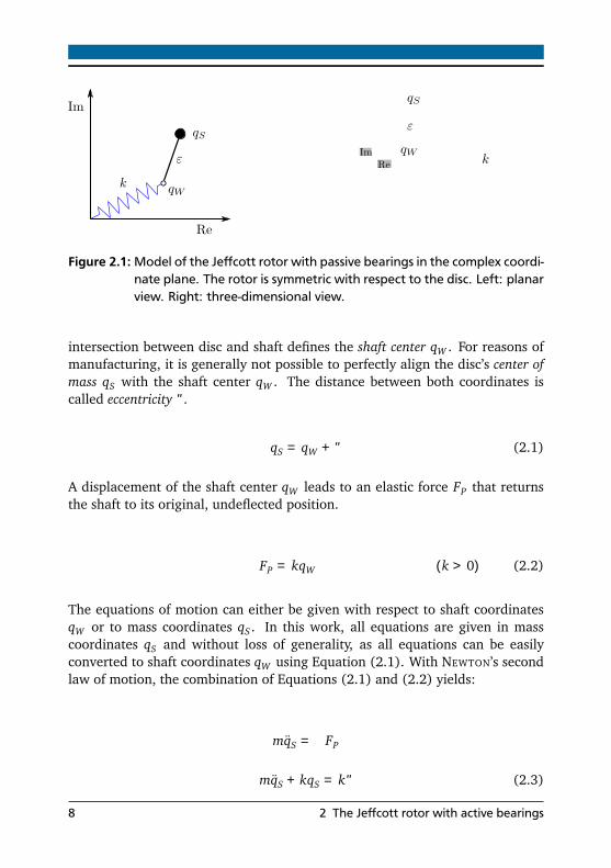
Figure 2.1: Model of the Jeffcott rotor with passive bearings in the complex coordi-nate plane. The rotor is symmetric with respect to the disc. Left: planarview. Right: three-dimensional view.

intersection between disc and shaft defines the shaft center qW . For reasons ofmanufacturing, it is generally not possible to perfectly align the disc’s center ofmass qS with the shaft center qW . The distance between both coordinates iscalled eccentricity ϵ.

qS = qW + ϵ (2.1)

A displacement of the shaft center qW leads to an elastic force FP that returnsthe shaft to its original, undeflected position.

FP = kqW (k > 0) (2.2)

The equations of motion can either be given with respect to shaft coordinatesqW or to mass coordinates qS . In this work, all equations are given in masscoordinates qS and without loss of generality, as all equations can be easilyconverted to shaft coordinates qW using Equation (2.1). With NEWTON’s secondlaw of motion, the combination of Equations (2.1) and (2.2) yields:

mqS = −FP

mqS + kqS = kϵ (2.3)

8 2 The Jeffcott rotor with active bearings

It is further assumed that the rotor turns with the angular rotational speed Ω,and that angular rotor accelerations can be neglected.

Ω= const. (2.4)

The eccentricity is a quantity that is bound to the rotor. When the rotor turns,the eccentricity also changes periodically from the viewpoint of the inertial coor-dinate system. To facilitate its description, a positive rotating coordinate systemis introduced. It shares the same origin as the inertial coordinate system, butis turned by the angle ϕ = Ωt, with t being the time. All quantities givenin the positive rotating coordinate system are identified by the superscript “+”.From the viewpoint of the positive rotating coordinate system, the eccentricityis constant.

ϵ+ = const. (2.5)

Another advantage of complex coordinates is that coordinate system rotationsby ϕ can be performed by a simple multiplication with eiϕ [19], and a coor-dinate transformation of the eccentricity ϵ+ from rotating coordinates to fixedones, gives:

ϵ = ϵ+ eiΩt (2.6)

Combining Equations (2.3) and (2.6) leads to the differential equation of thepassive rotor:

mqS + kqS = kϵ+ eiΩt (2.7)

Mathematically, this is an ordinary differential equation with constant coeffi-cients that can be solved using the ansatz qS = q+

S eiΩt . From the theory oflinear equations, it is known that q+

S is constant, and its second derivativeis qS = −q+

SΩ2 eiΩt . The solutions for the mass center qS and for the shaft

center qW can be simplified with the introduction of the natural frequencyω0 =

pm−1k. According to Equation (2.2), the passive bearing forces are

directly proportional to the displacements of the shaft center qW .

2.1 Mechanical properties of the passive system 9

qS =

−Ω2m+ k−1

kϵ+ eiΩt =

ω20 −Ω

2−1

ω20ϵ

+ eiΩt (2.8)

qW =

−Ω2m+ k−1

mΩ2ϵ+ eiΩt =

ω20 −Ω

2−1

Ω2ϵ+ eiΩt (2.9)

The Equations (2.8) and (2.9) give the solutions for mass and shaft center dis-placements. For low rotational speeds Ω ≪ ω0, both shaft displacements andbearing forces remain small, while the center of mass qS rotates around thebearing centerline and describes a circle with the radius |ϵ|. When the ro-tational speed Ω approaches the rotor’s natural frequency ω0, the quantities|qS |, |qW | as well as the bearing forces |FP | become very large. For Ω = ω0, therotor has reached its critical speed, and all quantities lean towards infinity withincreasing time. Operating a rotor at its critical speed without sufficient damp-ing is generally not recommended. In the late 19th century, engineers believedthat the rotor’s critical speed could never be passed. It was DE LAVAL who firstpractically demonstrated that a critical speed could be passed. For rotationalspeeds Ω > ω0, rotor displacements and forces become smaller. JEFFCOTT de-scribed this as “The effect of want of balance” in his pioneering work [53]. Forvery high rotational speeds Ω ≫ ω0, the mass center approaches the bearingcenterline qS → 0, while the shaft center qW circles around it.

Solving a differential equation requires the superposition of a particular solu-tion and a homogeneous solution. In case of a rotor, the first one describes theunbalance response, while the latter one describes the rotor’s natural vibra-tion. The homogeneous solution can be calculated when the right-hand side ofEquation (2.7) is set to zero:

q0 = q+O eiω0 t +q−O e−iω0 t (2.10)

The homogeneous solution q0 is a superposition of two complex quantities de-fined in different coordinate systems. The quantity q+

O is constant in the positiverotating coordinate system, while the solution q−O is constant in the negative ro-tating coordinate system, rotating in the opposite direction. Throughout thiswork, the superscript “−” represents quantities defined in the latter coordinatesystem. Both values depend on the initial conditions and are independent ofthe unbalance excitation.


2.2 The Jeffcott rotor with active bearings

Figure 2.2: Model of the actively supported Jeffcott rotor. The active bearing isrepresented by an arrow (red) that can move the flexible shaft (blue)in the complex plane. Left: 2D-projection of the extended Jeffcott rotorwith active bearings. Right: 3D representation.

As the name already indicates, the purpose of both active and passive bearingsis to bear or support the rotor, keeping it in its intended position. The JEFFCOTT

rotor is a statically determinate system. The forces on a bearing are reactionforces, they only depend on shaft loading. Imagine a planar rotor with a con-stant load FG on its disc, caused for example by gravity. Under static conditions,the bearing has to develop a reaction force FL of exactly the same magnitude sothat the sum of both vanishes, FG + FL = 0. Failure to deliver this force leads tostatic instability, regardless of whether the bearing is passive or active, or howsophisticated the underlying control algorithm might be.

Since in statically determinate systems the bearing loads only depend on theshaft forces, active bearings have no opportunity to alter them. In consequence,an active bearing cannot exert arbitrary forces on a rotor, as it leads to staticinstability. However, what active bearings can control is the shaft displacementin the complex plane, as they are able to move the rotor in the complex plane.Figure 2.2 illustrates a model of the JEFFCOTT rotor with active bearings. The redarrow depicts the displacements a of the active bearing in the complex plane.For now, this displacement is thought of as a purely abstract quantity. The goal isa strict separation between system-theoretic considerations and their physicalrealization, given in Chapter 4. With the actuator displacement a, the activebearing force F is:

2.2 The Jeffcott rotor with active bearings 11

F = k (qW − a) (2.11)

In analogy to Equation (2.7), the equation of motion is:

mqS + kqS = ka + kϵ (2.12)

The equation’s right-hand side only differs in the summand ka from its passivecounterpart. This summand requires special attention, as it contains productsof a stiffness k with the displacement quantities a and ϵ. In structural me-chanics, this product indicates a footpoint excitation or support excitation [102].Although the unit of the product ka is ‘Force’, the quantity physically representsa displacement excitation. Although replacing the expression ka with an ‘actu-ator force’ fa is mathematically correct, it leads to ambiguous, if not incorrectinterpretations of the physical realities. The only valid definition for the ac-tuator force is the one given in Equation (2.11). This important difference isclarified in an example of a rotor without eccentricity (ϵ = 0). The equationmqS + kqS = ka represents a rotor with active bearings at the shaft ends. In thiscase, the bearings are able to move the rotor in the complex plane without anyforces on the actuator or shaft. In contrast, if just the equation mqS +kqS = fa isgiven without further explanation, it might as well represent a system with fixedshaft ends and a force fa directly acting on the disc. Although both equationsare almost identical, they represent different physical setups with completelydifferent properties.

Given the findings in Equation (2.12), one can conclude that the evidence isnothing new. Moreover, the authors of standard literature on rotordynamicsand active bearings have found similar expressions [26, 29, 66]. The expressiona is usually named reference input and is either used for a static displacementcompensation or subsequently omitted. The presented approach differs fromthe standard one as the actuator displacement a is seen as dynamic control input,not a static compensation feature. The controller only uses the displacementsa to control the rotor. The advantage of this approach is that the conditionsfor static stability are automatically satisfied, leading to inherently consistentequations.


2.3 The controlled Jeffcott rotor

This section deals with the properties of the controlled rotor. After the deriva-tion of a new control algorithm, the rotor’s controlled unbalance response andits stability are thoroughly investigated.

2.3.1 Controller derivation

Figure 2.3: Illustration of the force free condition. The mass qS is kept still in therotational center without accelerations or forces. The shaft center qW

performs a circular motions, while the bearing displacement a followsthis motion, keeping the shaft in an undeflected position.

In this section, a new control algorithm that eliminates unbalance-induced bear-ing forces is derived. According to NEWTON’s second law of motion, the mass isforce free when it is kept at the rotational center, qS = 0. In this case, the shaftcenter qW performs according to Equation (2.1) and (2.6) circular motions withthe radius |ϵ+| around the rotational center, qW = −ϵ. However, no forces onthe mass also requires an unbent shaft, so according to Equation (2.11), theactuator displacement a and the shaft center qW must be coincident.

a = qW = −ϵ (2.13)

Figure 2.3 illustrates the kinematics of this force free condition. The designof an algorithm that meets this condition is challenging due to the followingreasons:

2.3 The controlled Jeffcott rotor 13

• The eccentricity ϵ changes periodically with the rotational speed Ω fromthe viewpoint of the inertial coordinate system.

• Although the eccentricity ϵ+ is constant in rotating coordinates, it is gen-erally unknown and unavailable for the control algorithm.

• The rotor movement is a combination of the unbalance response and thefree rotor vibration, hence a superposition of homogeneous and particu-lar solution. The controller has not only to alter the unbalance response,but also to stop the free vibration.

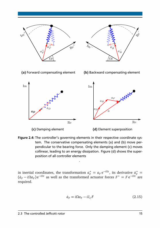
Considering the findings from Figure 2.3 it is clear that the rotor is in a forcefree condition when the actuator displacement is exactly opposite to the ec-centricity (a = −ϵ) so that the center of mass remains still in the rotationalcenter (qS = 0). The fact that the eccentricity ϵ+ is constant in the positivecoordinate system leads to the idea to define a controller with a displacementelement a+

F in rotating coordinates. In order to reach a force free condition, thisdisplacement control element must be opposite to the eccentricity (a+

F = −ϵ+).Although it is clear that this steady-state condition must be finally reached, it isunclear how to do so. The controller should always be able to converge to thisforce free condition, a demand which is closely linked to the stability of the con-trolled rotor. A system can be considered stable when its overall energy balanceis negative [74]. When this is the case, the free vibration’s energy will finallyvanish and the movement will stop. As a minimum requirement, the displace-ment element a+

F should not excite the rotor by introducing energy. Accordingto the principle of work, no power will be transferred to the mechanical systemwhen the velocity a+

F is geometrically perpendicular to the bearing force F+.This reasoning was conditionally inspired by conservative gyroscopic moments,which are energy-neutral because the involved moments and velocities are alsoperpendicular to each other. Figure 2.4a illustrates the situation, where the ve-locity a+

F causes a “spiral dive” of the mass. The control law of the conservativeforward compensation element a+

F is then:

a+F = −i cC F+ (2.14)

Throughout this work, i =p−1 represents the imaginary unit, and reflects

here the property of perpendicularity. The real parameter cC represents theadaption speed of the controller element. To express the controller equations


Although the controller element will not destabilize the system, it will not stabi-lize the rotor either – the homogeneous solution will not vanish. This behaviorshould not surprise as the controller element was specifically designed to beconservative. The stabilization of the controlled system requires a dissipatingcontroller element, depicted in Figure 2.4c. Its differential equation resemblesa mechanical spring-damper system.

aD = cD (F − kDaD) (2.16)

The parameter cD represents an inverse damping coefficient, while the factorkD is the stiffness of a fictitious return spring. A superposition of both controllerelements is able to finally stabilize the system. However, this stability is onlyconditional as it depends on both the rotor properties as well as the exact choiceof controller parameters. The problem of conditional stability is present in manyunbalance compensation algorithms [10, 55, 60], a unwanted property thatinhibits a broad application of these algorithms.

The stability of the controlled system depends on the eigenvalues of the ho-mogeneous differential equation and is independent of the rotor’s unbalanceresponse. It is interesting that the rotor’s free vibration solution from Equa-tion (2.10) consists of two parts. One is defined in positive rotating coor-dinates, whereas the other one is defined in the negative rotating coordinatesystem. The superposition of these counterrotating pointers leads to a symmetryin the homogeneous solution.

A supposition is that the controller’s conditional stability is caused by compen-sation element a+

F that is only defined in the positive rotating coordinate system.This asymmetric pointer might disturb the rotor’s initial symmetric solution. Theidea is to symmetrize the controller by introducing a second compensating elementa−B that is defined in the negative rotating coordinate system.

a−B = +i cC F− (2.17)

Figure 2.4b depicts the element’s governing equation. In analogy to Equa-tion (2.15), a transformation to the inertial coordinate system yields:


aB = −iΩaB + i cC F (2.18)

The controller is governed by three superpositioned elements as Figure 2.4dindicates. The forward compensation element a+

F from Equation (2.15), thebackward compensation element a−B from Equation (2.18), and the dampingelement aD deduced in Equation (2.16). A state-space representation conve-niently gathers all controller elements.

˙⎡

⎣

aFaBaD

⎤

⎦

xR

=

⎡

⎣

iΩ 0 00 −iΩ 00 0 −cDkD

⎤

⎦

AR

⎡

⎣

aFaBaD

⎤

⎦

xR

+

⎡

⎣

−i cC+i cC

cD

⎤

⎦

BR

F

a =

1 1 1

CR

xR (2.19)

The controller uses the bearing or actuator force F as control input while itcontrols the bearing displacement a. Figure 2.2 indicates that force and dis-placement are bound to the same degree of freedom. In this case, the sen-sor / actuator pair is collocated, a generally favorable property for controlledsystems [30]. Standard controllers have fixed parameters, but in case of Equa-tion (2.19), the system matrix AR is adaptive as it depends on the rotationalspeed Ω. The controller’s adaptive structure was derived through the coordi-nate transformations from rotating to inertial coordinates in Equations (2.15)and (2.18), based on the kinematic considerations from Figure 2.3 and Equa-tion (2.13). In contrast to many publications where an adaptive algorithm isan a-priori choice [10, 55, 60], the controller’s adaptive structure here wasthe logic result from kinematic considerations. A prerequisite for a successfulcontrol is accurate knowledge of the rotational speed Ω.

2.3.2 Unbalance response

Combining the actively supported rotor from Equation (2.12) with the con-troller from Equation (2.19) using the bearing force Equation (2.11) leads tothe state-space description of the controlled rotor:


˙⎡

⎢

⎢

⎢

⎢

⎣

qS

qS

aF

aB

aD

⎤

⎥

⎥

⎥

⎥

⎦

x

=

⎡

⎢

⎢

⎢

⎢

⎣

0 1 0 0 0−m−1k 0 m−1k m−1k m−1k−i cC k 0 iΩ+ i cC k icC k icC kicC k 0 −i cC k −iΩ− i cC k −i cC kcDk 0 −cDk −cDk −cD (k + kD)

⎤

⎥

⎥

⎥

⎥

⎦

A

⎡

⎢

⎢

⎢

⎢

⎣

qS

qS

aF

aB

aD

⎤

⎥

⎥

⎥

⎥

⎦

x

+

⎡

⎢

⎢

⎢

⎢

⎣

0m−1kicC k−i cC k−cDk

⎤

⎥

⎥

⎥

⎥

⎦

B

ϵ

x = Ax+Bϵ+ eiΩt (2.20)

In principle, the derivation of the rotor’s controlled unbalance response is sim-ilar to the calculation of the rotor’s passive response from Equation (2.9),with the difference that the ansatz is now a vector and not a constant. Withx = x+ eiΩt and its derivative x = iΩx+ eiΩt , the unbalance response is definedas:

x+ = (iΩI−A)−1 Bϵ+ (2.21)

Throughout this work, I represents the identity matrix of adequate dimensions.The particular solution exists if (iΩI−A) is invertible, which is the case when:

det (iΩI−A) = −2cC kΩ3 (iΩ+ cDkD) (2.22)

A solution exists when the rotor is rotating Ω = 0 and all other parametersare real and non-zero. This result differs from the uncontrolled JEFFCOTT rotorfrom Equation (2.9) which is singular when the rotational frequency matchesthe rotor’s eigenfrequency Ω = ω0. It can be concluded that the controlledrotor has no no resonance for any rotational speed Ω. The explicit solution ofEquation (2.21) requires a symbolic inversion of the (5× 5) matrix (iΩI−A).To avoid a tedious symbolic inversion, a particular solution x+ can be guessed,followed by a check of whether the preliminary solution solves Equation (2.20).According to Figure 2.3, a force free steady-state solution requires that the massremains still in the rotational center, so that both qS and qS must be zero andfurthermore according to Equation (2.13) – the negative eccentricity −ϵ mustmatch the actuator displacement a. The latter one is a superposition of three


controller elements a+F , a−B and aD, but since the eccentricity ϵ+ is defined in

the positive rotating coordinate system, it is assumed that the controller el-ement a+

F compensates the unbalance displacement entirely. Meanwhile, theother elements a−B and aD remain at zero. With these assumptions, the initialhypothetical solution is as follows:

x+ =

0 0 −ϵ+ 0 0T

(2.23)

It is now checked if the preliminary solution satisfies the equation:

(iΩI−A)x+ = Bϵ+

⎡

⎢

⎢

⎢

⎣

. . . . . . 0 . . . . . .

. . . . . . −m−1k . . . . . .

. . . . . . −i cC k . . . . . .

. . . . . . i cC k . . . . . .

. . . . . . cDk . . . . . .

⎤

⎥

⎥

⎥

⎦

(iΩI−A)

⎡

⎢

⎢

⎢

⎣

00−ϵ+

00

⎤

⎥

⎥

⎥

⎦

x+

=

⎡

⎢

⎢

⎢

⎣

0m−1kicC k−i cC k−cDk

⎤

⎥

⎥

⎥

⎦

B

ϵ+ (2.24)

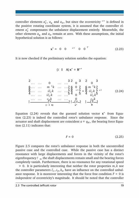
Equation (2.24) reveals that the guessed solution vector x+ from Equa-tion (2.23) is indeed the controlled rotor’s unbalance response. Since theactuator and shaft displacement are coincident a = qW , the bearing force Equa-tion (2.11) indicates that:

F = 0 (2.25)

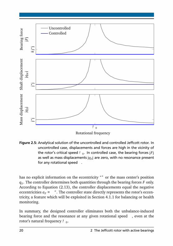
Figure 2.5 compares the rotor’s unbalance response in both the uncontrolledpassive case and the controlled case. While the passive case has a distinctresonance with large displacements and forces in the vicinity of the rotor’seigenfrequencyω0, the shaft displacements remain small and the bearing forcescompletely vanish. Furthermore, there is no resonance for any rotational speedΩ > 0. It is particularly interesting that neither the rotor properties m, k northe controller parameters cC , cD, kD have an influence on the controlled unbal-ance response. It is moreover interesting that the force free condition F = 0 isindependent of eccentricity’s magnitude. It should be noted that the controller


k|ϵ|

Bea

ring

forc

e|F|

UncontrolledControlled

|ϵ|

Shaf

tdi

spla

cem

ent

|qW|

ω0

|ϵ|

Rotational frequency Ω

Mas

sdi

spla

cem

ent

|qS|

Figure 2.5: Analytical solution of the uncontrolled and controlled Jeffcott rotor. Inuncontrolled case, displacements and forces are high in the vicinity ofthe rotor’s critical speed ω0. In controlled case, the bearing forces |F |as well as mass displacements |qS | are zero, with no resonance presentfor any rotational speed Ω.

has no explicit information on the eccentricity ϵ+ or the mass center’s positionqS . The controller determines both quantities through the bearing forces F only.According to Equation (2.13), the controller displacements equal the negativeeccentricities aF = −ϵ. The controller state directly represents the rotor’s eccen-tricity, a feature which will be exploited in Section 4.1.1 for balancing or healthmonitoring.

In summary, the designed controller eliminates both the unbalance-inducedbearing force and the resonance at any given rotational speed Ω, even at therotor’s natural frequency ω0.


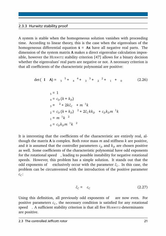
2.3.3 Hurwitz stability proof

A system is stable when the homogeneous solution vanishes with proceedingtime. According to linear theory, this is the case when the eigenvalues of thehomogeneous differential equation x = Ax have all negative real parts. Thedimension of the system matrix A makes a direct eigenvalue calculation impos-sible, however the HURWITZ stability criterion [47] allows for a binary decisionwhether the eigenvalues’ real parts are negative or not. A necessary criterion isthat all coefficients of the characteristic polynomial are positive:

det (λI−A) = α5λ5 +α4λ

4 +α3λ3 +α2λ

2 +α1λ+α0 (2.26)

α5 = 1

α4 = cD (k + kD)

α3 = Ω2 + 2kcCΩ+ m−1k

α2 = cD (k + kD)Ω2 + 2cC kkDΩ+ cDkDm−1k

α1 = m−1kΩ2

α0 = cDkDm−1kΩ2

It is interesting that the coefficients of the characteristic are entirely real, al-though the matrix A is complex. Both rotor mass m and stiffness k are positive,and it is assumed that the controller parameters cD and kD are chosen positiveas well. Some coefficients of the characteristic polynomial have odd exponentsfor the rotational speed Ω, leading to possible instability for negative rotationalspeeds. However, this problem has a simple solution. It stands out that theodd exponents of Ω exclusively occur with the parameter cC . In this case, theproblem can be circumvented with the introduction of the positive parametercC :

cC = ΩcC (2.27)

Using this definition, all previously odd exponents of Ω are now even. Forpositive parameters cC , the necessary condition is satisfied for any rotationalspeed Ω. A sufficient stability criterion is that all five HURWITZ-determinants ∆are positive.


∆1 = cD (k + kD) > 0

∆2 = cDk2

2cCΩ2 + m−1

> 0

∆3 = c2Dk2

2cC (k + kD) + 4c2C kkD

Ω4 + 4cC kkDm−1Ω2 + kkDm−2

> 0

∆4 = 2cC c2Dk4m−1Ω6 > 0

∆5 = 2cC c3Dk5kDm−2Ω8 > 0

The HURWITZ-determinants are all positive for controller parameters cC , cD, kD >0. This is the proof that the controlled system is always stable, independent ofthe rotor or controller parameters. Interestingly, the controlled system is evenasymptotically stable at the passive rotor’s natural frequency ω0. Althoughthe property of inherently stable control systems was extensively studied byPOPOV and called hyperstability or passivity [13], the concept primarily focusedat standard controllers with mostly damping properties. It is the author’s un-derstanding that the unique combination of an unbalance force elimination andhyperstability has not yet been reported or proven.

2.3.4 The secrets of hyperstability

The controller’s property of unlimited stability for positive controller parame-ters is a key finding of this work, and also a feature that sets it apart from other,conditionally stable control approaches. This remarkable stability property shallbe further investigated in this section. During the controller derivation in Sec-tion 2.3.1, it was revealed that the combination of two counterrotating com-pensating and a damping element finally led to unlimited stability. Apparently,a controller with one compensating element leads only to conditional stability.In order to better understand the secrets of unconditional stability, a controllerwith only one compensating element and conditional stability is compared withthe hyperstable controller from the previous section.

˙aFaD

=

iΩ 00 −cDkD

aFaD

+

−i cCcD

F

a =

1 1

aF aD

T(2.28)


10−3

100

103

Ω= 2π · 50 s−1

Mag

nitu

de[a/F]

Conditionally stableHyperstable

0 10 20 30 40 50 60 70 80 90 100−180

−135

−90

−45

0

Rotational frequency f (Hz)

Phas

ean

gle

()

Figure 2.6: Comparison of example frequency response functions for a condition-ally stable and a hyperstable controller for a rotational frequency Ω =2π50 s−1. The minor magnitude differences give no explanations as towhy one controller is hyperstable while the other is not.

Equation (2.28) gives the shortened, conditionally stable controller with onlyone compensating element defined in the positive rotating coordinate system aFand a damping element aD. In a first test, the controller’s closed-loop stability isinvestigated using its characteristic polynomial. Although the dimensions of thesystem matrix A are now (4× 4) and therefore smaller than the original (5× 5)system from Equation (2.20), its characteristic polynomial is more complicatedand also contains complex entries. For stability, all HURWITZ-determinants areregarded as positive. However, the results find out that:

∆2 = k2m−2

−mcC c2Dk2

D i + cDkD −Ωi −mcDΩ2

Looking at the last summand −mcDΩ2, it is clear that the closed-loop system

may become unstable, whereas the HURWITZ-determinants of the hyperstablecontroller (2.19) were always positive. In control engineering, frequency re-sponse functions or BODE plots are used to characterize the controllers [93] inthe frequency domain. Figure 2.6 gives the frequency response function forthe hyperstable controller from Equation (2.19) and the conditionally stable


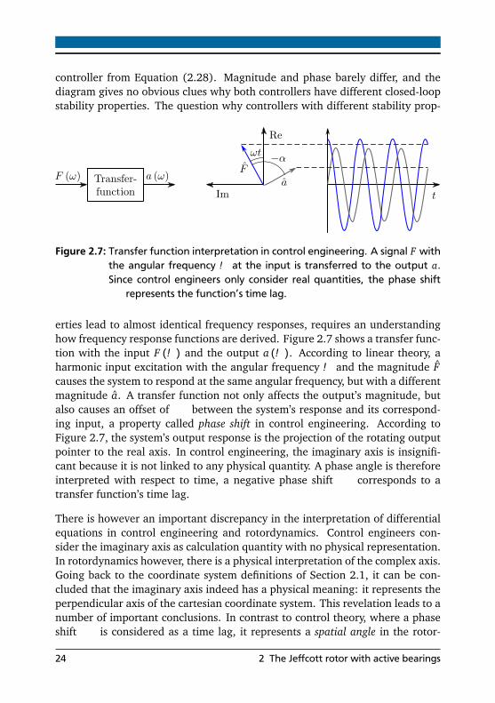
controller from Equation (2.28). Magnitude and phase barely differ, and thediagram gives no obvious clues why both controllers have different closed-loopstability properties. The question why controllers with different stability prop-masses which is depicted in figure ??.

Figure 2.7: Transfer function interpretation in control engineering. A signal F withthe angular frequency ω at the input is transferred to the output a.Since control engineers only consider real quantities, the phase shift−α represents the function’s time lag.

erties lead to almost identical frequency responses, requires an understandinghow frequency response functions are derived. Figure 2.7 shows a transfer func-tion with the input F (ω) and the output a (ω). According to linear theory, aharmonic input excitation with the angular frequency ω and the magnitude Fcauses the system to respond at the same angular frequency, but with a differentmagnitude a. A transfer function not only affects the output’s magnitude, butalso causes an offset of −α between the system’s response and its correspond-ing input, a property called phase shift in control engineering. According toFigure 2.7, the system’s output response is the projection of the rotating outputpointer to the real axis. In control engineering, the imaginary axis is insignifi-cant because it is not linked to any physical quantity. A phase angle is thereforeinterpreted with respect to time, a negative phase shift −α corresponds to atransfer function’s time lag.

There is however an important discrepancy in the interpretation of differentialequations in control engineering and rotordynamics. Control engineers con-sider the imaginary axis as calculation quantity with no physical representation.In rotordynamics however, there is a physical interpretation of the complex axis.Going back to the coordinate system definitions of Section 2.1, it can be con-cluded that the imaginary axis indeed has a physical meaning: it represents theperpendicular axis of the cartesian coordinate system. This revelation leads to anumber of important conclusions. In contrast to control theory, where a phaseshift −α is considered as a time lag, it represents a spatial angle in the rotor-


dynamic complex coordinate system, which also changes the interpretation ofthe frequency response function. In control engineering, negative frequenciesrepresent acausal systems which require knowledge of future events. On thecontrary this perspective makes sense from a rotordynamic view. When positivefrequencies represent a rotor rotating in the mathematically positive directionof rotation in the complex plane (forward whirling), negative frequencies rep-resent the shaft rotating in the mathematically negative direction of rotation(backward whirling). In this interpretation, negative frequencies do not repre-sent future events, but only a change in the direction of rotation.

10−3

100

103

Ω= 2π · 50 s−1

Mag

nitu

de[a/

F]

−75 −50 −25 0 25 50 75−180

−90

0

90

180


Phas

ean

gle

()

HyperstableConditionally stable

Figure 2.8: Two-sided frequency response functions for both controllers. In rotor-dynamics, negative frequencies ω < 0 do not represent future events,but rather rotations in mathematically negative direction. In contrastto the conditionally stable controller, its hyperstable counterpart is sym-metrical in the complex plane, explaining its unique stability properties.

Figure 2.8 depicts a two-sided frequency response function and extends theone-sided version from Figure 2.6 to negative frequencies. Although both con-trollers are almost equal for ω > 0, differences become apparent for negativefrequenciesω< 0. In contrast to its conditionally stable counterpart, the hyper-stable controller has a symmetry in the complex plane. In this case, the phaseangle does not represent a time lag, but spatial information about the directionbetween the inputs and outputs in the complex plane.


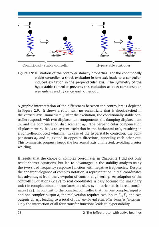
It can be concluded that the one-sided transfer function from Figure 2.6 canexplain the controlled rotor’s unbalance response, but is unable to explainthe controller’s superior stability properties. In contrast to control engineer-ing where the imaginary axis is physically meaningless, the latter represents aphysical dimension in rotordynamics. Under this changed paradigm, negativefrequencies as well as phase angles are interpreted not in a time, but in a spatialcontext. The symmetry of the two-sided frequency response function depictedin Figure 2.8 finally explains the controller’s unique stability properties. In realcoordinates, the controller requires four non-trivial transfer functions. The rea-son of the controller’s stability properties lies in the special controller coupling ofthe rotor axes.


3 General rotors withactive bearings

The ideas of the previous chapter are now extended to general rotor systems.After a revision of the rotor’s elastic properties and its passive unbalance re-sponse, the research turns to a thorough investigation of the kinematics forrotors with active bearings. Using the controller from the previous section, aclosed-loop state-space model is built. The controlled unbalance response iscalculated. Two examples demonstrate that the controller allows for a forcefree operation and an elimination of resonances even for arbitrary rotors. Theapproach is extended to rotors with gyroscopy and damping, and the influenceof parasitic stiffnesses as well as the bearing placement is discussed. In manyapplications not only the rotor, but also the bearing foundations are flexible.The chapter’s last topic gives also a solution for this common problem.

The contents as well as some figures of this chapter are based on the publication“Unbalance and resonance elimination with active bearings on General Rotors”written by HEINDEL et al. [39].

3.1 Mechanical model

This section derives the matrix properties of elastic rotors, discusses the rotor’spassive behavior and finally highlights the characteristics of flexible rotors withactive bearings.

3.1.1 Elastic properties of free rotors

Throughout this section, the theoretical analysis and the derivation of the ro-tor’s characteristic elastic features are demonstrated on a slender beam, ac-centuating the connection between physical and mathematical properties. It isstressed that the following considerations are manifested on, but not limitedto this particular beam structure. The continued use of complex notation lim-its the considerations to isotropic rotors only. This limitation is motivated in

29

The relation between displacements qW and corresponding node forces FR isgiven by HOOKE’s law.

FR = KRqW (3.2)

(a) Beam translation

(b) Beam rotation

Figure 3.2: The free beam can be translated and rotated without any node forces.

Symmetry is not the only exploitable property of the stiffness matrix. Objectscan be moved or turned as a whole. These movements cause no internal stressesand deformations, leaving the object as it is, and are subsequently called rigidbody motions. Figure 3.2 shows these cases. Although never explicitly de-rived, this special property is already included in the stiffness matrix. Bothshaft translations qW t and rotations qW r leave the shaft unbent and cause nobearing forces [67].

0 = KRqW t , 0 = KRqW r (3.3)

A general three-dimensional body has six rigid body modes, three translationsplus the same quantity of rotations. Since rotor movements in axial directionare neglected and the rotor rotates around one axis with the rotational angleΩt, only four rigid body modes remain. These split up in one translational androtational mode for each plane. The use of complex notation already accountsfor two perpendicular axes, so only two vectors are needed to represent fourrigid body motions.

From the mathematical viewpoint, the matrix KR is a linear map that relates thedisplacement vector qW to the force vector FR. A deduction of Equation (3.3)

3.1 Mechanical model 31

is that the stiffness matrix KR maps any linear combination of qW t and qW r tothe null vector. This property is named rank deficiency, and since the (p× p)matrix KR maps two linear independent eigenvectors to the null vector, its rankdeficiency is two [3].

rank (KR) = p− 2 (3.4)

This makes KR singular, making it impossible to determine the shaft displace-ments qW when only the node forces FR are known. Another implication is thattwo eigenvalues of KR are zero. These two zero eigenvalues correspond to onefree translation and rotation. In real coordinates, the shaft’s stiffness matrixwould have four zero eigenvalues.

Stiffness matrices are normally generated with finite elemente software, suchas Nastran or Ansys. Many programs generate stiffness matrices that have notonly translational, but also rotational degrees of freedom. For these matrices, astatic condensation technique eliminates the unnecessary rotational degrees offreedom [67, 103]. Matrices with rotational degrees of freedom will be consid-ered in Section 3.2.6.

3.1.2 The rotor with passive bearings

The distribution of matter on a real rotor is continuous, but for modeling pur-poses, these distributions are discretized by a finite number of masses. One canimagine this discretization as if the real rotor was cut into slices. Each slicehas a different weight and center of gravity, represented by point masses inthe model. When the slices get thinner, the model reaches higher fidelity, butalso gets more complex and more difficult to handle. In many cases, the rotor’smasses are not evenly distributed, but concentrate on specific elements, suchas discs, fans, impellers, etc. whereas the interconnecting shaft is thin. Thenit is often sufficient to consider each of these features as a total number of ppoint masses connected to a massless shaft. The coordinates of the centers ofgravities qS1, . . . , qSp are gathered in the (1× p) vector qS , while the mass pointsm1, . . . , mp are joined in the mass matrix M. The further considerations do notaccount for massless nodes, so it is demanded that M is regular.

It is practically impossible to perfectly align the slices’ centers of gravity to theshaft, leading to small residual eccentricities ϵ+1 , . . . ,ϵ+p , which are all gatheredin the rotor-fixed eccentricity vector ϵ+. Analogous to Equation (2.1), the rela-tion between fixed and rotating coordinate system is:

32 3 General rotors with active bearings

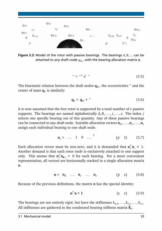
Figure 3.3: Model of the rotor with passive bearings. The bearings A, B, ... can beattached to any shaft node qW j with the bearing allocation matrix n.

ϵ = ϵ+ eiΩt (3.5)

The kinematic relation between the shaft nodes qW , the eccentricities ϵ and thecenter of mass qS is similarly:

qS = qW + ϵ (3.6)

It is now assumed that the free rotor is supported by a total number of z passivesupports. The bearings are named alphabetically A, B, . . . , j, . . . , z. The index jselects one specific bearing out of this quantity. Any of these passive bearingscan be connected to any shaft node. Suitable allocation vectors nA, . . . ,n j , . . . ,nzassign each individual bearing to one shaft node.

n j =

. . . 1 0 . . .T

(p× 1) (3.7)

Each allocation vector must be non-zero, and it is demanded that nTj n j = 1.

Another demand is that each rotor node is exclusively attached to one supportonly. This means that nT

j n = j = 0 for each bearing. For a more convenientrepresentation, all vectors are horizontally stacked in a single allocation matrixn.

n =

nA . . . n j . . . nz

(p× z) (3.8)

Because of the previous definitions, the matrix n has the special identity:

nT n = I (z × z) (3.9)

The bearings are not entirely rigid, but have the stiffnesses kLA, . . . , kL j , . . . , kLz .All stiffnesses are gathered in the condensed bearing stiffness matrix KL .


KL = diag

kLA, . . . , kL j , . . . , kLz

(z × z) (3.10)

For all following considerations, it is demanded that each stiffness element kL j

is positive, making KL regular. Finally, the diagonal and spare bearing stiffnessmatrix KL can be defined.

KL = nKLnT (p× p) (3.11)

The careful definition of the matrices n, KL and KL is important as many futureresults make extensive use of the defined matrices and their identities. Since thebearings are attached to the shaft, they both share the same coordinate vectorqW . The passive bearing forces FP that act on the shaft are then:

FP = KLqW (3.12)

For static stability, it is further assumed that the rotor is supported in a statically(in-)determinate manner. This condition is satisfied when the rotor is supportedat least in two bearing planes. The total system stiffness matrix is then positivedefinite, which is signalized using the “>” symbol:

KR +KL > 0 (3.13)

Two basic forces act on the mass. The rotor’s elastic forces FR that were definedin Equation (3.2) and the passive bearing forces FP defined in Equation (3.12).Applying NEWTON’s second law of motion yields:

MqS = −FP − FR (3.14)

As already stated in Section 2.1, the equations of motion can be either expressedin shaft coordinates qW or in mass coordinates qS . Although books on basicrotordynamics introduce both variants [26, 64], shaft coordinates qW are com-monly used. For the sake of a comprehensive presentation, the following resultsare presented in mass coordinates qS . This is without loss of generality, sincethe coordinates can be transformed from one system to the other. With theeccentricity definition from Equation (3.5) and the kinematic relations fromEquation (3.6), the equation of motion is:

MqS + (KR +KL)qS = (KR +KL)ϵ+ eiΩt (3.15)


In analogy to Section 2.1, the unbalance response is calculated using the har-monic ansatz qS = q+

S eiΩt in vectorized form.

qS =

−Ω2M+ (KR +KL)−1

(KR +KL)ϵ+ eiΩt (3.16)

A modal transformation helps to understand the solution’s properties. The de-composition M−1(KR+KL) = UPVPU−1

P can be applied where the diagonal matrixVP stores the p squared eigenfrequencies of the passive system:

VP = diag

ω2P1, . . . ,ω2

Pp

(3.17)

Both M and the total stiffness matrix (KR +KL) are positive, real and symmetric[25]. The eigenvectors are then orthogonal and can be normalized in a way thatU−1

P = UTP . Through the decomposition Equation (3.16), the system simplifies

to p modal oscillators.

qS = UP

VP −Ω2I−1

VPUTP ϵ

+ eiΩt

= UP diag

ω2P1

ω2P1 −Ω2

, . . . ,ω2

Pp

ω2Pp −Ω2

UTP ϵ

+ eiΩt (3.18)

An analysis of Equation (3.18) indicates that the diagonal entries become verylarge when the rotational frequency Ω approaches the system’s eigenfrequen-cies ωp. When the both frequencies match exactly , the solution is no longervalid: the resonance requires a different type of ansatz. When the rotationalspeed Ω is raised even further so that it is higher than the system’s eigenfre-quencies ωp, the diagonal entries get smaller again and finally approach zero.It is interesting though that the sign shifts as the resonance is passed. Close tothe resonance, the mass deflections qS become very large. The correspondingshaft displacements qW are calculated with Equation (3.6).

qW = UP

VP −Ω2I−1

VP − I

UTP ϵ

+ eiΩt

= UP diag

Ω2

ω2P1 −Ω2

, . . . ,Ω2

ω2Pp −Ω2

UTP ϵ

+ eiΩt (3.19)

The shaft deflections qW behave similarly to the mass deflections qS derived inEquation (3.18). Both have in common that they become very large close to


the rotor’s resonance frequency, and that they change their sign from positiveto negative. From Equation (3.12) it is clear that the passive bearing forcesare directly proportional to the shaft deflections, FP = KLqW . The followingstatements summarize the main results of the rotor with passive bearings.

• For a given rotational speed Ω, the system’s force response behaves lin-early. Doubling the eccentricity ϵ also doubles the bearing forces FP .

• A rotor system with p degrees of freedom has p resonances.

• In the vicinity of a resonance, both rotor deflections qW and passive bear-ing forces FP are very high.

• The p resonance frequencies ω1, . . . ,ωp depend on the properties of therotor as well as on the bearings, including their quantity, position andstiffness.

3.1.3 The rotor with active bearings

It is now assumed that the free rotor from Section 3.1.1 is now supported byactive bearings. In analogy with the controlled JEFFCOTT rotor, they are also rep-resented by abstract displacement quantities. Generally speaking, both activeand passive bearings need to hold a rotor in its designated position. Withoutbearings, the rotor would just move through space under the influence of exter-nal forces, a behavior which is almost never desired. The purpose of a bearingis to oppose these forces to keep the rotor in its desired position.

Similar to their passive counterparts, active bearings are unable to modify theforces on a statically determinate rotor. A rotor displacement causes a bear-ing reaction force as an effect, not vice versa. This fact raises the question ofwhat active bearings can actually control. Unable to change the rotor forcesdirectly, they can control the rotor displacements. In a statically determinateconfiguration, active bearings are able to actively translate and rotate the rotorwithout bearing forces. These force free movements occur in two perpendicularplanes, leading to four degrees of freedom. It must be stressed that this prop-erty does not depend on the active bearings’ physical realization. Whether theyare based on piezoelectricity, magnetic effects, or other technological realiza-tions, all forms are able to statically move the rotor without forces. The abilityto move the rotor without constraints depends only on the system’s topology.

Figure 3.4 illustrates the rotor with active bearings. Each active bearing A, . . . , zis able to displace the rotor; the displacement vectors aA, . . . , az are represented


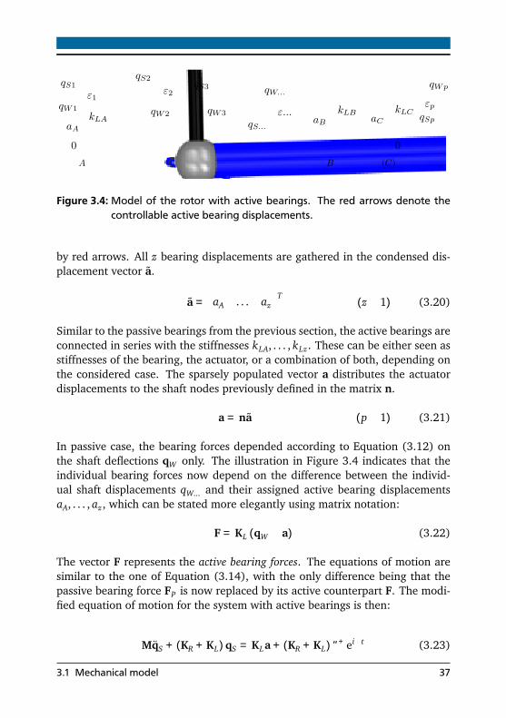
Figure 3.4: Model of the rotor with active bearings. The red arrows denote thecontrollable active bearing displacements.

by red arrows. All z bearing displacements are gathered in the condensed dis-placement vector a.

a =

aA . . . az

T(z × 1) (3.20)

Similar to the passive bearings from the previous section, the active bearings areconnected in series with the stiffnesses kLA, . . . , kLz . These can be either seen asstiffnesses of the bearing, the actuator, or a combination of both, depending onthe considered case. The sparsely populated vector a distributes the actuatordisplacements to the shaft nodes previously defined in the matrix n.

a = na (p× 1) (3.21)

In passive case, the bearing forces depended according to Equation (3.12) onthe shaft deflections qW only. The illustration in Figure 3.4 indicates that theindividual bearing forces now depend on the difference between the individ-ual shaft displacements qW... and their assigned active bearing displacementsaA, . . . , az , which can be stated more elegantly using matrix notation:

F = KL (qW − a) (3.22)

The vector F represents the active bearing forces. The equations of motion aresimilar to the one of Equation (3.14), with the only difference being that thepassive bearing force FP is now replaced by its active counterpart F. The modi-fied equation of motion for the system with active bearings is then:

MqS + (KR +KL)qS = KLa+ (KR +KL)ϵ+ eiΩt (3.23)


The only difference between the passive equation of motion (3.14) and theactive one is the actuator displacement summand KLa on the equation’s right-hand side. In analogy to the JEFFCOTT rotor from Section 2.2, the active bearingsstimulate the rotor via a footpoint excitation [92]. The right-hand side expres-sion requires special attention: although the unit of KLa is ‘force’, it does notrepresent an actual force. The right-hand side expression KLa is nonzero andmay lead to the tempting but false conclusion that the right-hand side expres-sion actually represents a real physical force excitation. This false conclusionmight sneak in gradually: the expression KLa might be renamed as an ‘activebearing force’. Although this substitution is mathematically faultless, it pavesthe way to wrong conclusions about the system’s physical realities. A moredetailed treatment of this topic is given in Section 4.2.

When the free rotor is supported in more than two bearing planes, it is staticallyindeterminate. In this case, individual actuator displacements cause shaft bend-ing and consequently impose forces on the bearings. This behavior is alreadycovered by Equation (3.23). It is revealed later that a force free operation isguaranteed even when the rotor is supported by active bearings in a staticallyindeterminate manner.

3.2 The controlled rotor

During the study of the JEFFCOTT rotor in Chapter 2, an inherently stable adap-tive controller was introduced. This controller did not only eliminate the bear-ing forces, but also removed the rotor’s resonance. These special propertiesseemed interesting enough to apply the control algorithm to general, isotropicrotors with an arbitrary number of masses and stiffnesses.

3.2.1 Control approach

In Section 3.1.3, the mechanical model for an arbitrary rotor with a total num-ber of z active bearings was introduced. It is now assumed that each activebearing is equipped with its own, individual controller. The state-space nota-tion for this controller is identical to the one given in Equation (2.19), but sincethe subindices have changed, it is repeated here for completeness:


˙⎡

⎣

aF jaB jaD j

⎤

⎦

xRj

=

⎡

⎣

iΩ 0 00 −iΩ 00 0 −cD jkD j

⎤

⎦

ARj

⎡

⎣

aF jaB jaD j

⎤

⎦

xRj

+

⎡

⎣

−i cC j+i cC j

cD j

⎤

⎦

BRj

F j

a j =

1 1 1

CRj

xRj (3.24)

The force of the j-th active bearing is denoted as F j , while a j is the actuatordisplacement (represented by the red arrow in Figure 3.4) of the same activebearing. Since all controllers are independent from each other, they are allarranged in a block-diagonal matrix structure:

˙⎡

⎣

xRAxRB

...

⎤

⎦

xR

=

⎡

⎣

ARA 0 00 ARB 0

0 0. . .

⎤

⎦

AR

⎡

⎣

xRAxRB

...

⎤

⎦

xR

+

⎡

⎣

BRA 0 00 BRB 0

0 0. . .

⎤

⎦

BR

⎡

⎣

FAFB...

⎤

⎦

F

aRA aRB . . .T

a

= diag (CRA,CRB, . . . )

CR

xR (3.25)

The state vector xR has the dimensions (3z × 1). Similar to the relation betweenthe condensed actuator displacements a with the actuator displacements a innode coordinates from Equation (3.21), the condensed bearing forces F gatherthe forces FA, . . . , Fz of all z bearings and are related to the node bearing forcesF in the following manner:

F = nT F (z × 1) (3.26)

3.2 The controlled rotor 39

3.2.2 Unbalance response of the controlled system

Both the mechanical system with active bearings as well as the controller havebeen defined in Sections 3.1.3 and 3.2.1. Both are now joined in a single state-space system for further analysis of the system’s unbalance response. The com-bined state vector x together with Equations (3.6), (3.22) and the combinationof Equations (3.23)-(3.26) leads to the combined state-space description:

˙⎡

⎢

⎣

qS

qS

xR

⎤

⎥

⎦

x

=

⎡

⎢

⎣

0 I 0

−M−1 (KR +KL) 0 M−1KLnCR

BRnT KL 0 AR −BRnT KLnCR

⎤

⎥

⎦

A

⎡

⎢

⎣

qS

qS

xR

⎤

⎥

⎦

x

+

⎡

⎢

⎣

0

M−1 (KR +KL)

−BRnT KL

⎤

⎥

⎦

B

ϵ

x = Ax+Bϵ (3.27)

The state-space representation of Equation (3.27) is composed of many subma-trices. However, the large monolithic structure of the system matrix A can bedecomposed into several blocks, where each block has its unique designation.The (2p× 2p) matrix in the upper-left corner represents the equation of motionfor the mechanical system. The controller resides in the (3z × 3z) matrix in thelower-right corner. The controller influences the mechanical systems throughactuators, where the (2p× 3z) matrix on the upper-right corner connects thecontrollers states to the mechanical degrees of freedom. In the lower-left cor-ner, the (3z × 2p) sensor matrix feeds the mechanical displacements back to thecontroller.

Linear theory states that a harmonic unbalance excitation ϵ = ϵ+ eiΩt causes thesystem to respond at exactly the same frequency. Similar to the passive solu-tion of Equation (3.15), a similar harmonic ansatz can be used to calculate thesystem’s unbalance response. The unbalance response is assumed to satisfy theequation x = x+ eiΩt , with x+ being a constant vector for a particular rotationalspeed Ω. Its derivative yields x = iΩx+ eiΩt . Combining these harmonic re-sponses with the system’s state-space notation x = Ax+Bϵ leads to the wantedsolution when (iΩI−A) is invertible:

x = (iΩI−A)−1 Bϵ (3.28)


Although the solution of Equation (3.28) is theoretically straightforward, onehas to remember that the system matrix A is a block matrix of the dimension(2p + 3z), which has to be inverted. A relatively simple system with p = 3masses and z = 2 active bearings already requires the inversion of a matrixwith the dimensions (10× 10). The comprehensible solution for the controlledJEFFCOTT rotor in Section 2.3.2 encouraged the search for a solution on arbi-trary rotors, and finding a general solution is one of the key elements of thiswork. Due to its length, the detailed calculation is moved to Appendix A.1, buta brief description of the necessary steps is also given here. The system matrixA is divided into a mechanical, controller, sensor and actuator part. The matrixinversion lemma [104] allows for a problem simplification because the parti-tioned smaller matrix blocks can be calculated separately. Finding a general yetsimple solution heavily relies on the structure of the involved matrices. Suitablematrix definitions in the Sections 3.1.1 and 3.2.1 allow for the application ofthe WOODBURY Matrix Identity, finally leading to a comprehensive, yet simplesolution.

x(t) =

⎡

⎢

⎣

−Ω2M+KR

−1KR

iΩ

−Ω2M+KR

−1KR

RnT

−Ω2M+KR

−1KR −RnT

⎤

⎥

⎦ϵ+ eiΩt (3.29)

The steady-state unbalance response given in Equation (3.29) contains the ma-trix R, which was defined during the solution process in Appendix A.1, but isrepeated here for convenience. The diagonal matrix R = diag(r, r, . . . ) con-tains z column vectors r =

1 0 0T

. The implications of the unbalanceresponse (3.29) are successively reviewed in detail, and starts with the discus-sion of the mass motion:

qS =

−Ω2M+KR

−1KRϵ

+ eiΩt

When the rotor motion of the active solution is compared to its passive coun-terpart from Equation (3.16), remarkable similarities can be observed: the onlyformal difference between the active solution and the passive one is that itlacks the bearing stiffness matrix KL , while the rest remains exactly the same. Amodal decomposition gives a better understanding of the rotor behavior. Sup-pose that UVUT is the modal decomposition of M−1KR. With this decomposition,V is:


V = diag

0,0,ω21, . . . ,ω2

p−2

(3.30)

Two diagonal entries of V are zero, leading to two zero matrix rows and colums.The reason for this property can be traced back to the matrix product of M−1KR.It was stated earlier that the free rotor has two rigid body modes. Accordingto Equation (3.4), these are reflected in a rank deficiency of two in the rotor’sstiffness matrix KR. The inequality states that the rank deficiency of KR alsoaffects the matrix product:

rank(M−1KR)≤min

rank(M−1), rank(KR)

= p− 2 (3.31)

This rank deficiency is the reason why the diagonal eigenvalue matrix (3.30)holds at least two zero diagonal entries. The equations of motion for the massesare then:

qS = U

V−Ω2I−1

VUTϵ+ eiΩt

= Udiag

0,0,ω2

1

ω21 −Ω2

, . . . ,ω2

p−2

ω2p−2 −Ω2

UTϵ+ eiΩt (3.32)

The two zero diagonal entries from Equation (3.32) indicate that the systemlacks two resonances. The passive system from Equation (3.18) had p reso-nances, leading to theoretically infinite deflections and forces when the rota-tional speed Ω matches any of these p resonance frequencies. In the activecase, the deflections lean to infinity for only p − 2 frequencies. Consequently,the controller enables the elimination of two rotor resonances. This behavior canbe traced back to the rank deficiency of Equations (3.4) and (3.31), which orig-inated in the free shaft’s property to rotate and tilt without node forces. Theshaft deflections qW are then:

qW = U

V−Ω2I−1

V− I

UTϵ+ eiΩt

= Udiag

−1,−1,Ω2

ω21 −Ω2

, . . . ,Ω2

ω2p−2 −Ω2

UTϵ+ eiΩt (3.33)


Comparing the passive solution from Equation (3.19) with the active one fromEquation (3.33) illustrates how the rotor’s motion differs. In the passive case,the rotor displacements qW → 0 are negligible for small rotational speedsΩ → 0. In latter case, the diagonal entries (−1) indicate that the shaft ex-ecutes circular movements with the magnitude of the eccentricity ϵ, whereasEquation (3.32) expresses that the mass movements qS are approximately zero.As a conclusion, the active control system displaces the rotor in a way that thecenter of masses always stay in the rotational center. Some more interestingproperties can be found when the controller states xR from Equation (3.29) arereviewed:

xR =

RnT

−Ω2M+KR

−1KR −RnT

ϵ+ eiΩt

Finally, the kinematic relations between the shaft and mass displacements fromEquation (3.6) allow the following simplifications:

xR = RnT

qS − ϵ+ eiΩt

= RnT qW (3.34)

Consequently, the controller states xR directly depend on the shaft coordinatesqW . This property gets clearer when it is not the states, but the individual con-troller outputs which are observed. According to Equation (3.25), the relationbetween the condensed actuator displacements a and the controller states xR isa = CRxR. This expression leads to the product of the block-matrices CR and R,which results in the identity matrix I. The use of Equation (A.9) leads to thecondensed actuator displacements:

a = CRRnT qW = nT qW (3.35)

It is now clear that the actuator displacement matches the shaft displacement attheir respective nodes. In steady-state, the actuator movements follow exactlythe shaft movements. This is particularly interesting as it has consequences forthe actuator forces. Equation (3.22) demonstrated that the active bearing forcesF are the difference between the actuator displacement and shaft displacement.Using the relation a = na from Equation (3.21) allows the calculation of thebearing forces:


F = KL (qW − a) = KLqW −KLnnT

=KL

qW = 0 (3.36)

Equation (3.36) is the proof that the bearing forces in steady-state are always zero.This result is considered as one of the key elements in this work. It is particularsurprising because of the following reasons: apart from the basic definitionsin Section 3.1.1, no further assumptions were made on the stiffness, shape ormass of the rotor. It is further surprising given that the force free condition isindependent of the eccentricity vector ϵ. The control algorithm has no specificknowledge about the mass distribution, yet is able to control the actuators in away that the bearing forces vanish. The result is valid for all rotational speedsΩ. The control algorithm does not require any information about the rotoror the mechanical setup, i.e. the bearing’s position or stiffness, since only therotational speed Ω must be known.

• For a given rotational speed Ω, the system’s active bearing force responseremains zero for any unbalance distribution ϵ+.

• Two resonances can be eliminated – a passive rotor system with p degreesof freedom has p− 2 resonances in controlled case.

• In the vicinity of a free rotor resonance, the deflections qW become large,but the active bearing forces F remain zero.

• The p − 2 resonance frequencies ω1, . . . ,ωp−2 depend on the propertiesof the free rotor only. The number of active bearings as well as theirposition or stiffness have no effect on the rotor’s unbalance response.

3.2.3 Example rotor with two discs

An example illustrates the solution derived in the previous section. The consid-ered rotor consists of two discs attached to a flexible shaft. Figure 3.5 showsthe mechanical setup, but in contrast to the illustration, it is assumed that theactive bearings support the rotor directly at the disc location. The mass matrixM has then the dimension (2× 2), and according to the rank deficiency of thefree rotor found in Equation (3.4), it is clear that the rank of the rotor’s stiff-ness matrix is zero. Consequently, the rotor’s stiffness matrix KR is also zero,representing the fact that both nodes are completely independent from eachother as the shaft translates and tilts without constraints. The system with two


(a) 1st passive resonanceat frequency fP1

(b) 2nd passive resonanceat frequency fP2

Figure 3.5: Uncontrolled (passive) rotor with two discs. In passive operation, twodiscs lead to two resonances with distinct eigenmodes.

masses essentially degenerates to two controlled, uncoupled JEFFCOTT rotors.The bearing stiffness matrix KL is assumed to be diagonal, but with differentstiffnesses for two distinct passive eigenfrequencies. Figure 3.7 compares rotorrun-ups in passive and active cases. Two distinct resonances develop at the fre-quencies fP1 and fP2 in the passive case. There are no resonances in the activecase because the controller is able to always align the center of both masses inthe rotational center, as Figure 3.6 indicates. The bearing forces vanish becausein steady-state operation, the actuator displacements a j follow exactly the shaftmovement qW j at the corresponding node. This example pursues two different

Figure 3.6: Controlled (active) rotor with two discs. The rotor is resonance-free forany rotational speed Ω due to the masses remaining in the center ofrotation.


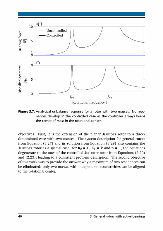
01

5

10·k|ϵ|

Bea

ring

forc

e|F|


fP1 fP201

5

10·|ϵ|

Rotational frequency f

Dis

cdi

spla

cem

ent

|qW|

Figure 3.7: Analytical unbalance response for a rotor with two masses. No reso-nances develop in the controlled case as the controller always keepsthe center of mass in the rotational center.

objectives. First, it is the extension of the planar JEFFCOTT rotor to a three-dimensional case with two masses. The system description for general rotorsfrom Equation (3.27) and its solution from Equation (3.29) also contains theJEFFCOTT rotor as a special case: for KR = 0, KL = k and n = 1, the equationsdegenerate to the ones of the controlled JEFFCOTT rotor from Equations (2.20)and (2.23), leading to a consistent problem description. The second objectiveof this work was to provide the answer why a maximum of two resonances canbe eliminated: only two masses with independent eccentricities can be alignedto the rotational center.


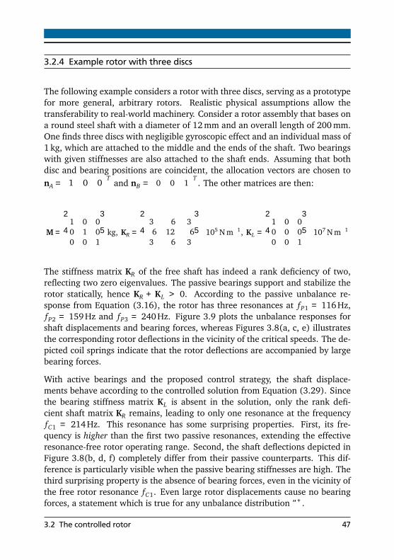
3.2.4 Example rotor with three discs

The following example considers a rotor with three discs, serving as a prototypefor more general, arbitrary rotors. Realistic physical assumptions allow thetransferability to real-world machinery. Consider a rotor assembly that bases ona round steel shaft with a diameter of 12 mm and an overall length of 200 mm.One finds three discs with negligible gyroscopic effect and an individual mass of1 kg, which are attached to the middle and the ends of the shaft. Two bearingswith given stiffnesses are also attached to the shaft ends. Assuming that bothdisc and bearing positions are coincident, the allocation vectors are chosen tonA =

1 0 0T

and nB =

0 0 1T

. The other matrices are then:

M =

⎡

⎣

1 0 00 1 00 0 1

⎤

⎦kg, KR =

⎡

⎣

3 −6 3−6 12 −63 −6 3

⎤

⎦ · 105 N m−1, KL =

⎡

⎣

1 0 00 0 00 0 1

⎤

⎦ · 107 N m−1

The stiffness matrix KR of the free shaft has indeed a rank deficiency of two,reflecting two zero eigenvalues. The passive bearings support and stabilize therotor statically, hence KR + KL > 0. According to the passive unbalance re-sponse from Equation (3.16), the rotor has three resonances at fP1 = 116Hz,fP2 = 159 Hz and fP3 = 240 Hz. Figure 3.9 plots the unbalance responses forshaft displacements and bearing forces, whereas Figures 3.8(a, c, e) illustratesthe corresponding rotor deflections in the vicinity of the critical speeds. The de-picted coil springs indicate that the rotor deflections are accompanied by largebearing forces.

With active bearings and the proposed control strategy, the shaft displace-ments behave according to the controlled solution from Equation (3.29). Sincethe bearing stiffness matrix KL is absent in the solution, only the rank defi-cient shaft matrix KR remains, leading to only one resonance at the frequencyfC1 = 214 Hz. This resonance has some surprising properties. First, its fre-quency is higher than the first two passive resonances, extending the effectiveresonance-free rotor operating range. Second, the shaft deflections depicted inFigure 3.8(b, d, f) completely differ from their passive counterparts. This dif-ference is particularly visible when the passive bearing stiffnesses are high. Thethird surprising property is the absence of bearing forces, even in the vicinity ofthe free rotor resonance fC1. Even large rotor displacements cause no bearingforces, a statement which is true for any unbalance distribution ϵ+.


(a) 1st passive resonanceat frequency fP1

(b) No resonance with controlat frequency fP1.

(c) 2nd passive resonanceat frequency fP2

(d) No resonance with controlat frequency fP2.

(e) 3rd passive resonanceat frequency fP3

(f) Force-free resonance with controlat frequency fC1.

Figure 3.8: Graphical comparison of a rotor with three discs in passive (left column)and active case (right column). Three critical frequencies develop in thepassive case, leading to high bearing forces. With active bearings, onlyone force free resonance develops (Figure f).


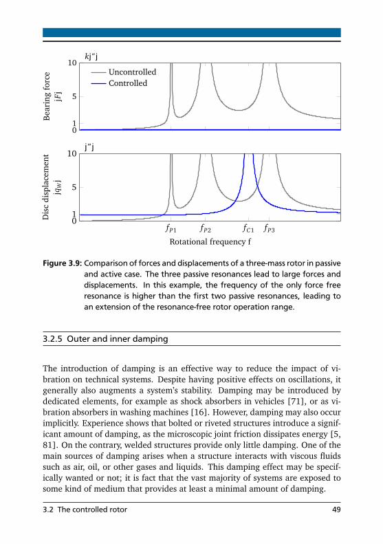
01

5

10·k|ϵ|

Bea

ring

forc

e|F|


fP1 fP2 fC1 fP301

5

10·|ϵ|


Dis

cdi

spla

cem

ent

|qW|

Figure 3.9: Comparison of forces and displacements of a three-mass rotor in passiveand active case. The three passive resonances lead to large forces anddisplacements. In this example, the frequency of the only force freeresonance is higher than the first two passive resonances, leading toan extension of the resonance-free rotor operation range.

3.2.5 Outer and inner damping

The introduction of damping is an effective way to reduce the impact of vi-bration on technical systems. Despite having positive effects on oscillations, itgenerally also augments a system’s stability. Damping may be introduced bydedicated elements, for example as shock absorbers in vehicles [71], or as vi-bration absorbers in washing machines [16]. However, damping may also occurimplicitly. Experience shows that bolted or riveted structures introduce a signif-icant amount of damping, as the microscopic joint friction dissipates energy [5,81]. On the contrary, welded structures provide only little damping. One of themain sources of damping arises when a structure interacts with viscous fluidssuch as air, oil, or other gases and liquids. This damping effect may be specif-ically wanted or not; it is fact that the vast majority of systems are exposed tosome kind of medium that provides at least a minimal amount of damping.


Figure 3.10: Rotor with external damping. Although external damping reducesfree rotor deflections, it creates a parallel path to the environment.This parallel path transmits forces to the ambiance, voiding the rotor’sforce free operation.

Since some amount of damping is generally unavoidable, the implications ofits occurrence are studied in this section. Rotordynamic theory distinguishesbetween two kinds of damping: outer or external damping and inner damping.Outer damping results from the rotor’s interaction with the fixed environmentand has the effect that a mechanical engineer would expect – it reduces the rotorvibrations and augments the rotor’s stability margin. On the other hand, innerdamping describes the rotor’s intrinsic dissipation. Surprisingly, inner dampinghas an adverse effect on stability, leading to the paradox effect that augmentingthe rotors’ inner damping eventually leads to instability. It took decades andmany damaged or destroyed rotors until this negative effect could finally beendeciphered by NEWKIRK and KIMBALL. Statements about the stability of innerdamping are generally hard, but will be discussed briefly in Section 5.1.7. It ishowever possible to study both the effects of outer and inner damping on theunbalance response and their effect on the force free operation.

External damping is defined in the inertial coordinate system. The dampingforces act on the rotor, and the most obvious approach is that the dampingforces are directly proportional to the shaft velocities qW . For the sake of sim-plicity and presentation, it is assumed here that the damping forces act directlyon the masses. Even though this case allows a detailed discussion about thegeneral effects, as this change only affects the right-hand side of the state-spaceequation. The damping force vector FD is assumed to be directly proportional tothe absolute mass velocities qS . Because of energy considerations, the external


damping matrix is symmetric, so D = DT . Figure 3.10 illustrates the externaldamping arrangement.

FD = DqS (3.37)

Inner damping is entirely defined in rotating coordinates. The inner dampingforces defined in the positive rotating coordinate system F+

I are directly pro-portional to the mass velocities q+

S . The inner damping matrix DI must satisfythe same energy considerations and is symmetric also: DI = DT

I . For innerdamping, the governing equation is:

F+I = DI q

+S (3.38)

Before Equation (3.38) can be incorporated in the equation of motion, it hasto be transferred first to the inertial coordinate system. The transformation forthe force vector from fixed to rotating coordinates yields F+

I = FI e−iΩt . Thedisplacement transformation is then: q+

S = qS e−iΩt . Its derivative requires theproduct rule: q+

S = qS e−iΩt −iΩqS e−iΩt . With these replacements, the equationfor the inner damping can be expressed in inertial coordinates:

FI = DI qS − iΩDIqS (3.39)

The transformation to inertial coordinates creates not only a velocity-dependentquantity, but also one which is proportional to the displacement qS . Until now,position-dependent forces were only used in conjunction with conservative elas-tic elements. In Section 3.1.1, the principle of virtual works led to symmetryin the stiffness matrices, see Equation (3.1). However, the product iΩDI isskew-hermitian, (Hermitian matrices are the complex equivalent to symmet-ric real matrices) and consequently not conservative. The existence of thisskew-hermitian matrix identifies systems with circulatory forces. Consideringall forces, the equation of motion yields:

MqS = −F− FR − FD − FI

This leads to an updated state-space description. Compared to the state-spacenotation in Equation (3.27), only the system matrix A has changed, while thematrix B remains the same. If the assumptions were changed in a way that the


damping is proportional to the shaft displacement qW , the matrix B also wouldhave changed.

A =

⎡

⎢

⎣

0 I 0

−M−1 (KR +KL − iΩDI ) −M−1 (D+DI ) M−1KLnCR


⎤

⎥

⎦(3.40)

A solution for the state-space system of Equation (3.27) with the updated sys-tem matrix from Equation (3.40) that involves outer and inner damping hasbeen calculated in Appendix A.2. The result from Equation (A.28) is also pre-sented here:

x(t) =

⎡

⎢

⎣

−Ω2M+ iΩD+KR

−1KR

iΩ

−Ω2M+ iΩD+KR

−1KR

RnT

−Ω2M+ iΩD+KR

−1KR −RnT

⎤

⎥

⎦ϵ+ eiΩt (3.41)

External damping: Comparing the unbalance response for the undamped sys-tem from Equation (3.29) with the solution of the damped case from Equa-tion (3.41), shows that only marginal changes occurred in the dynamic stiffnessmatrix

−Ω2M+ iΩD+KR

, where only the summand iΩD is new. A modalsolution is only indicated when the matrix D is also diagonalizable with theeigenvectors of the undamped system, otherwise the solution gets more com-plicated [25]. However, some important properties are known even without anexplicit modal solution. Damping leaves the number of resonances unaffected,the controlled system has only p − 2 resonances. Furthermore, the introduc-tion of damping limits the modal displacements from infinite to finite valuesin the resonance. Repeating the calculation from Equation (3.36) reveals thatthe bearing forces F remain zero. Both results are generally appreciated, butimply a severe drawback. Looking again at Figure 3.10, it is apparent that thedamping elements give a twofold response. The same damping force FD thatacts on the rotor also requires a reaction force of the same magnitude on theenvironment. Even though the active bearings are in a force free condition,oscillatory forces may still be transmitted to the environment through a paral-lel path. A necessary requirement for a complete rotor isolation is the absenceof any external damping D = 0, but this implies large rotor deflections in thevicinity of a free rotor resonance, as it was demonstrated in Equation (3.18). It


is clear that this property depends on the rotor only and has nothing to do withthe controller, as its properties are not part of the unbalance response.

As a corollary, it is generally impossible to operate a rotor at the speed of its freeresonance and fully eliminate the bearing forces it at the same time.

Internal damping: Although the inner damping matrix DI appeared in the sys-tem matrix A from Equation (3.40), it is not present in the unbalance responsefrom Equation (3.41). This is no mistake; it turns out that the unbalance re-sponse remains indeed unaffected by inner damping. This surprising result hasa plausible explanation. A closer inspection of the unbalance response fromEquation (A.28) indicates that the relation between rotor-fixed, constant eccen-tricity vector ϵ+ and rotor displacements in rotating coordinates q+

S is actuallyconstant. When observed from the rotating coordinate system, the rotor de-flects statically, and for a given rotational speed Ω no movement can be seen.According to Equation (3.38), inner damping was also defined in rotating co-ordinates, and the absence of any relative movements q+

S = 0 also causes thatthe inner damping forces on the rotor are zero, FI = 0. The name inner damp-ing already suggests that these forces do not interact with the environment,consequently inner damping allows for a complete force free rotor operation.Although it has no negative impact on the unbalance response, its occurrenceshould be avoided whenever possible. Its circulatory parts encourage instabilityfor passive rotors, and it is likely that this negative property also applies for thecontrolled system. Since the stability theorems of Chapter 5 do not apply forsystems with circulatory matrices, a numeric stability test is indicated for rotorswith suspected inner damping.

3.2.6 Gyroscopic effect and generalized coordinates

The modeling approach of Section 3.1.1 gives good results for slender rotors,but not so much for short and thick rotor shapes. STODOLA discovered more thana century ago that the cause for the deviation between model and experimentcould be attributed to the gyroscopic effect [89]. It was assumed previously thatthe rotor is cut into slices, and that the center of mass is represented as a pointwith an assigned eccentricity. For thick rotors, this assumption is inaccurate.The continuous mass distribution of one slice is not only reflected in a centerof mass, but also in a transversal moment of inertia Θt and a polar moment ofinertia Θp.


⎡

⎣

MP1...

MPp

⎤

⎦=

⎡

⎣

iΩΘP1. . .

iΩΘPp

⎤

⎦

G(Ω)

⎡

⎢

⎣

β1...βp

⎤

⎥

⎦(3.42)

The gyroscopic matrix changes with the rotational speed Ω, which means noth-ing else that the cross-coupling becomes stronger the faster the rotor spins. Forthe trivial case of that Ω= 0, the matrix vanishes and there is no coupling at all.In complex coordinates, the matrix G (Ω) is diagonal but imaginary. The mostimportant property is that the matrix is skew-hermitian.

G (Ω) = −GH (Ω) (3.43)

It seems that the introduction of transversal and polar moments of inertia com-plicate the equations of motions considerably. Previously, it was sufficient tocare about masses, displacements and forces. Now a whole new set of vari-ables appears, namely inertia, angles and moments, which are coupled throughthe gyroscopic effect. This raises the question of whether or not the previouslyfound solutions can be adapted in such a way, that they account for the neweffects. When the transversal moment was discussed earlier, it was already im-plied that the equations of motions for node rotations are in complete analogyto their displacement counterparts. During the derivation of the stiffness ma-trix in Section 3.1.1, it was already mentioned that a stiffness matrix may alsohave rotational degrees of freedom, but as they were superfluous, they could beremoved using static condensation.

Because of the structural analogy between translations and rotations, general-ized coordinates can be used to facilitate the problem description. The vector qSis extended so that it holds not only displacements qS but also the node rota-tions β . Then the matrix M does not only hold masses m, but also transversalmoments of inertia Θt , and the eccentricity vector ϵ+ does not only contain ec-centricities ϵ+, but also an error for skewed discs. The advantage of generalizedcoordinates is that the problem’s matrix formulation remains exactly the same,and all solutions found in Section 3 are also valid for generalized coordinates.Generalized coordinates allow the problem’s abstraction from a specific physicalsetup to the study of matrix properties. For instance, the rotor’s ability to move


freely is expressed in the rank deficiency of KR, independent if only displace-ments or displacements and rotations are used as governing coordinates.

Only the speed-dependent, gyroscopic moments have to be updated in the state-space matrix:

A =

⎡

⎢

⎣

0 I 0

−M−1 (KR +KL) −M−1 (D+G (Ω)) M−1KLnCR


⎤

⎥

⎦(3.44)

The solution has been calculated in Section A.1, but is also given here:

x(t) =

⎡

⎢

⎣

−Ω2M+ iΩ(D+G(Ω)) +KR

−1KR

iΩ


−1KR

RnT


−1KR −RnT

⎤

⎥

⎦ϵ+ eiΩt (3.45)

An eigenvalue decomposition for the complete M,D,G,K system is only possi-ble in special cases. When damping is omitted, the shortened M,G,K-systemcan be decomposed in complex coordinates. This decomposition leads to com-plex eigenvectors and a breakdown of the resonance frequencies into a forwardwhirling frequency and a backward whirling frequency. In real coordinates, adiagonalization is still possible when a bimodal decomposition that uses dif-ferent left and right eigenvectors, is applied [25]. More solution techniques,decomposition strategies and interpretations, are found in standard books onrotordynamics [26, 29].

The speed-dependent character of G(Ω) leads to a gyroscopic stiffening. Thiseffect is not a stiffening in the classical sense as it does not alter the rotor’s stiff-ness matrix, but describes that an augmentation in the rotor’s rotational speedΩ also leads to increased forward whirling frequencies ω. At the same time,the backward whirling frequencies diminish. In theory, rotor unbalances ϵ+ eiΩt

only excite the forward whirling frequencies, whereas the backward whirl doesnot contribute to the rotor’s unbalance response.

Gyroscopic moments are conservative and generally have unproblematic stabil-ity behavior, as it will be demonstrated in Section 5.2. But since the rotor’seigenvectors change for different rotational speeds, one must check carefully


whether the observability criteria of Section 5.2.4 are always satisfied. Gyro-scopic moments do not require any external reaction forces and are entirelybound to the rotor, hence a complete rotor isolation is possible. To simplifypresentation, the matrices’ G(Ω) explicit dependence of the rotational speed Ωwill be omitted, and only G will be used.

3.2.7 Parasitic stiffness

Figure 3.12: Parasitic stiffnesses inhibit a force free rotor operation and create newresonances. However, they can be compensated when they arise inthe active bearing planes.

Another effect which has not been considered yet is the presence of parasiticstiffnesses. Until now, it was assumed that active bearings are able to translateand tilt the rotor freely. There are cases where these conditions may not beentirely satisfied. Some machines feature elements that partially hinder a freerotor movement. In some cases, this may be a design feature, for example whenthe system is equipped with passive bearings. However, sometimes parasiticstiffnesses occur as a secondary effect, this happens for example for a flexiblecoupling whose primary purpose is the transmission of torque. Finally, eventhe active bearings may introduce parasitic stiffnesses. In case of displacementactuators, some extra stiffness may create a parallel path which is not measuredby the force sensors (see Section 4.1.4).

In this section, the properties of parasitic stiffnesses are investigated. Fig-ure 3.12 shows a sketch of the modified system with the additional springelements kS1, . . . , kSp. All are stored in the sparsely populated, diagonal ma-


trix KS . The forces that are transmitted to the environment via the parasiticstiffnesses are consequently:

FS = KSqW (3.46)

Parasitic stiffnesses remain unobserved by the active bearings, and the updatedstate space matrices are then:

A =

⎡

⎢

⎣

0 I 0

−M−1 (KR +KL +KS) 0 M−1KLnCR


⎤

⎥

⎦, B =

⎡

⎢

⎣

0

M−1 (KR +KL +KS)

−BRnT KL

⎤

⎥

⎦

Solving the system is straightforward as KR is now replaced by KR +KS .

x(t) =

⎡

⎢

⎣

−Ω2M+KR +KS

−1(KR +KS)

iΩ

−Ω2M+KR +KS

−1(KR +KS)

RnT

−Ω2M+KR +KS

−1(KR +KS)−RnT

⎤

⎥

⎦ϵ+ eiΩt (3.47)

A force free rotor operation always leads to some residual rotor movements.According to Equation (3.46), forces will be transmitted to the environment.The presence of a parasitic stiffness disables the possibility to completely isolatethe rotor. In Section 3.2.2, it was stated that two rotor resonances can be elimi-nated using active bearings. This effect was attributed to the rank deficiency ofKR in Equation (3.4), a property that reflected the rotor’s ability to move freely.In presence of parasitic stiffnesses, not the stiffness matrix KR determines thesolution properties, but the sum of KR + KS . When the rotor is supported notonly by an active bearing, but also by a passive one, only one resonance canbe eliminated as the rank (KR +KS) = p − 1. When the rotor is fully supportedby passive bearings, no resonance can be eliminated: the active bearings areuseless as they have no influence on the rotor’s unbalance response.

These parasitic resonances are particularly dangerous as they may occur at ro-tational frequencies that do neither match the eigenfrequencies of the free, un-constrained rotor nor the ones of the fixed rotor, and may be misidentified ascontroller instabilities.

Until now, it was assumed that the bearing force and the actuator force are oneand the same. For parasitic stiffnesses in the bearing plane, this is no longer thecase: the bearing force vector F differs from the actuator force vector Fa. Whenthe parasitic stiffness kS at the respective node is known, the control algorithm


may compensate it using the actuator. This enables a complete rotor isolationand resonance elimination even in the presence of these unwanted effects. InChapter 4, compensating strategies for force and displacement actuators arepresented.

In summary, the presence of parasitic stiffnesses counteracts all positive effectsthat may come from a controlled solution with active bearings: first, they estab-lish a parallel path that transmits unbalance forces to the surrounding, imped-ing a full rotor isolation. Second, they create new resonances that may occurat unexpected rotational frequencies. Third, they have no positive impact onthe resonance magnitudes. External damping in contrast limits the resonancepeaks and does not introduce new resonances. As a conclusion, parasitic stiff-nesses should be avoided whenever possible or compensated when they occurin a bearing plane.

3.2.8 Bearing invariance

(a) Controlled rotor with two bear-ings

(b) Controlled rotor with three bear-ings.

Figure 3.13: Bearing invariance: the rotor’s unbalance response is independent ofboth the number and the placement of the active bearings. This coun-terintuitive behavior can be explained by the absence of unbalance-induced bearing forces during steady-state operation.

The solution for the controlled shaft from Equation (3.29) does neither dependon the controller parameters nor on the matrix KL . This matrix contains not onlyinformation about the stiffness of each active bearing, but also stores accord-ing to Equation (3.11) the position where each individual bearing is attached.Consequently, the rotor’s controlled unbalance response depends neither on the


position nor the number of the used active bearings. This unintuitive steady-statebehavior makes sense, as the force free condition also implies that there is nointeraction between the rotor and the bearings. For the unbalance response,the rotor behaves as if there were no bearings. However, the system’s homo-geneous solution which governs the rotor’s natural vibration and damping iscertainly affected by active bearing placement, see Chapter 5.

Figure 3.13 depicts two identical rotor systems with the rotational frequencybut with different bearing locations. With either two or three bearings, andindependent of the the bearing location, the rotor’s unbalance response remainsthe same.

This bearing invariance property can be exploited when passing free rotor reso-nances. Details can be found in Section 4.4.

3.3 Rotor-casing interaction

In real-world machinery, rotor foundations and casings are rarely considered asfixed elements. Weight matters especially when rotating machines are part oftransport systems, such as cars, planes, rockets, and so on. To reduce weight,the rotor casings are built as light as possible, leading to softer structures withaugmented oscillation tendencies. But even large stationary rotating machinessuch as generators in power plants or steam turbines do not only excite theirthick-walled steel housing, but also the surrounding building. The rotor’s cas-ing excitation is not only a nuisance, but also affects the rotor behavior itself,leading to an interaction of both components. Neglecting the casing’s effect onthe rotor may lead to surprises when they are joined. The aforementioned situ-ation encouraged researchers to study the problem in detail [26] or to developsophisticated calculation methods [24].

Aircraft engines are particularly susceptible to this problem. The lightweightdesign of the engine cowling and fuselage encourages the transmissions ofunbalance-induced vibrations in the form of audible noises to passengers. BothBORSDORF and ZHAO investigated active elements to reduce unbalance-inducedengine vibrations with rotor-casing interactions [12, 101]. This section de-scribes the derivation of the unbalance response with a casing. In this section,the rotor coordinates are represented by the subindex “r” (rotor), whereas allcasing quantities are represented by the subindex “c” (casing). Both subsys-tems are joined in the combined system with the subindex “g”. The combineddisplacement vector qSg is then:


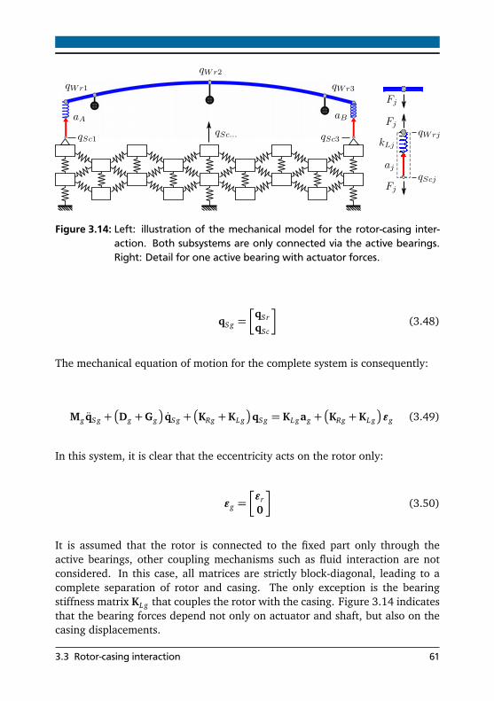
F = KL (qW r − qSc − a) (3.51)

Appendix A.4 demonstrates that only small modifications of the previously de-rived unbalance response are necessary to cover also this problem. Then, thecontrolled unbalance response for the mechanical system is:

qSg =

−Ω2Mg + iΩ

Dg +Gg

+KRg

−1KRgϵg (3.52)

The solution of Equation (3.52) shows that the bearing stiffness matrix KLg ,which coupled both systems, vanished. Since the remaining matrices are strictlyblock-diagonal, both systems are completely decoupled. Equation (3.50) re-vealed that the unbalance only acts on the rotor, consequently there is no exci-tation of the casing.

To illustrate the findings, the rotor with three masses from example 3.2.4 isnow attached to a lightly damped casing with multiple resonances in the rotor’soperating range. Since the passive stiffness matrix KRg +KLg is of full rank, thepassive system counts not only with three, but with rank(KRg +KLg) resonances.In these resonances the rotor excites the casing. In controlled case, no forcesare transmitted through the bearings, leading to a silent casing. However, thefree rotor resonance cannot be eliminated. Figure 3.15 illustrates a rotor run-upin passive and active case.


01

5

10·k|ϵ|

Bea

ring

forc

e|F|


01

5

10·|ϵ|

Rot

ordi

sp.

|qW

r|

fC101

5

10·|ϵ|


Cas

ing

disp

.|q

Sc|

Figure 3.15: Example for a rotor-casing interaction. The run-up of a rotor withthree discs excites the multiple resonance frequencies of the flexiblecasing in the passive case. In active case however, the absence of anybearing forces stops the casing vibration entirely, but a free rotor res-onance remains. A complete unbalance decoupling is possible evenwhen the rotor is attached to an arbitrary, flexible casing.

3.3 Rotor-casing interaction 63

4 Physical realizationUntil this point, the problem of a force free rotor operation was only consid-ered from system-theoretic viewpoint. The previous chapters dealt mainlywith the question how to control an ideal actuator so that a complete rotorisolation is possible. The abstract component focused on ensuring a completeseparation between the theoretic foundations and the active bearings’ practi-cal implementation. By first establishing the theoretical foundations and dis-cussing their physical properties, two immediate advantages are found: firstly,the system-theoretic considerations are of general nature and technology inde-pendent, widening the problem’s understanding. Second, by deriving controlstrategies for different technologies emerging from the same theory uncoversconnections that would be unnoticed otherwise. For a specific implementation,two major decisions have to be made.

The first decision concerns the actuator type. Independent of the particulartechnology used, actuators can be categorized into two idealized groups [32].The first group is formed by displacement actuators. These actuators have ide-ally an infinite inherent stiffness. For any given operating point, a change in theactuator force Fa leads to a negligible relative actuator displacement ∆a = 0.Corollary, any small actuator displacement ∆a leads to an infinite change inactuator forces Fa →∞. Latter group is formed by ideal force actuators whichhave no inherent stiffness. Without control, even a small change in the actuatorforces Fa leads to infinite displacements ∆a →∞, but displacements ∆a leavethe actuator forces Fa = 0 unchanged. The type of actuator naturally affectsthe required sensor. Collocated controllers require the knowledge of both forceand displacement for a respective node. Displacement actuators are invariantto changing forces. Hence only a force sensor may measure the unknown quan-tity. Force actuators on the other hand require a position measurement as theirforces are invariant to displacements. In conclusion, the measured quantitymust be complementary to the one of the actuator [30].

Figure 4.1 illustrates the behavior of real-world actuators that are only approx-imations to these idealizations. Displacement actuators have a finite stiffness,whereas force actuators might even have negative stiffnesses. Most actuatorsare located somewhere in between, and their characterization largely depends

65

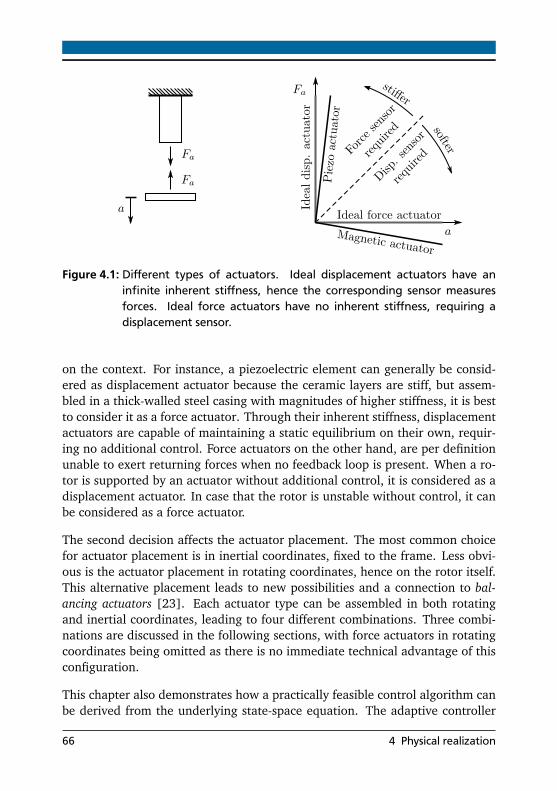
Figure 4.1: Different types of actuators. Ideal displacement actuators have aninfinite inherent stiffness, hence the corresponding sensor measuresforces. Ideal force actuators have no inherent stiffness, requiring adisplacement sensor.

on the context. For instance, a piezoelectric element can generally be consid-ered as displacement actuator because the ceramic layers are stiff, but assem-bled in a thick-walled steel casing with magnitudes of higher stiffness, it is bestto consider it as a force actuator. Through their inherent stiffness, displacementactuators are capable of maintaining a static equilibrium on their own, requir-ing no additional control. Force actuators on the other hand, are per definitionunable to exert returning forces when no feedback loop is present. When a ro-tor is supported by an actuator without additional control, it is considered as adisplacement actuator. In case that the rotor is unstable without control, it canbe considered as a force actuator.

The second decision affects the actuator placement. The most common choicefor actuator placement is in inertial coordinates, fixed to the frame. Less obvi-ous is the actuator placement in rotating coordinates, hence on the rotor itself.This alternative placement leads to new possibilities and a connection to bal-ancing actuators [23]. Each actuator type can be assembled in both rotatingand inertial coordinates, leading to four different combinations. Three combi-nations are discussed in the following sections, with force actuators in rotatingcoordinates being omitted as there is no immediate technical advantage of thisconfiguration.

This chapter also demonstrates how a practically feasible control algorithm canbe derived from the underlying state-space equation. The adaptive controller

66 4 Physical realization

structure leads to a different control law for each operating point, making astraightforward implementation difficult. A coordinate transformation tech-nique is presented which allows for an implementation of this controller even onmachines with very limited computational power. When the hazardous effectsof parasitic stiffnesses from Section 3.2.7 occur in the active bearing plane, theycan be compensated. Compensation techniques are presented for both displace-ment and force actuators. A practical implementation requires dimensioning ofthe actuators, and it is demonstrated how the closed-loop solution can be usedfor this purpose. The same solution also revealed that both rotor and actua-tor displacements may become very large close to the free rotor resonances -a property that is intolerable in real machines. The introduction of an addi-tional controller factor inhibits a perfect force free operation, but also reducesboth rotor and actuator displacements to tolerable values. The proposed factorlimits the travel of the compensation elements and leads to a blending of rotorisolation and the classical introduction of damping.

The displacement and force formulations in Sections 4.1.1 and 4.2 are based onthe publication “Unbalance and resonance elimination with active bearings ona Jeffcott Rotor” by HEINDEL et al. [38].

4.1 Displacement actuators

Displacement actuators with finite stiffness may be realized through differenttechnologies. For slowly turning machines with large eccentricities, the lowbandwidth of linear electric motors may be negligible. Machines with higherrotational speeds tend to smaller eccentricities, a domain where other actuatorprinciples have their advantages. Hydraulic actuators offer very high powerdensities, large strokes and bandwidths exceeding 100 Hz. For even higherfrequencies and smaller strokes, piezoelectric actuators qualify. They offerextremely high bandwidths in the kilohertz range [32], but their small strainof approximately 0.2 % leads to either long actuators or small strokes. Someless common actuator principles include magnetorestrictive actuators and shapememory alloys [52]. A special role have actuators that are based on thermalexpansion. They feature large forces, but have the drawbacks of very smallstrains and only quasi-static operation. However, they may still be suitable forunbalance elimination, as the upcoming sections will show.

4.1 Displacement actuators 67

Figure 4.2: Physical realization of an active bearing with displacement actuators.Each actuator displaces the bearing in one plane; the sensors directlymeasure the shaft forces.

4.1.1 Fixed displacement actuators

Following the previous theoretical derivations, an actuator assembly in inertialcoordinates is the most intuitive solution. Figure 4.2 shows such an assem-bly. A mechanical bearing that allows the shaft’s rotation while it prevents theshaft’s radial movements is connected in series with two perpendicularly ar-ranged linear displacement actuators. Each actuator is connected to a forcesensor; the assembly is then attached to a fixed support. Sample implemen-tations can be found in [6, 82, 88]. The controller outputs the displacementa in complex coordinates, consequently one actuator is fed by the real partRea, while its perpendicular counterpart is fed with Ima. The sensor in-puts ReF and ImF must be converted to complex coordinates using therelation F = ReF + i ImF, accordingly. Until now, there was no clear dis-tinction between bearing and actuator stiffness. This was perfectly justified asit made no difference from the system-theoretic viewpoint. If both shall beconsidered simultaneously, their total stiffness is simply defined by their seriesconnection.

In principle, the implementation of the controller from Equations (2.19)or (3.24) is straightforward. In practice however, many machines do not runat a constant rotational speed Ω, but rather change their rotational frequencyto operate at different operating points. In this case, the rotational speed Ωmust be measured using a resolver or an encoder. Thus, in these cases, the con-troller must be adaptive so that it can cover the machine’s different operatingpoints. This adaptive structure requires either a parametric model or different


controllers for each operating point. Both variants are rather tedious, makingtheir implementation on systems with little computational power difficult. Amore elegant solution takes advantage of the fact that the involved controllerelements were defined in different coordinate systems. The controller’s for-ward compensating element a+

F was defined in the positive rotating coordinatesystem, whereas the backward compensating element a−F was defined in thenegative rotating coordinate system, while the damping element aD was de-fined in inertial coordinates. With a modified state vector xR, the controllerdifferential equation can be transformed in a way that its explicit dependenceon the rotational speed Ω lapses.

xR =

a+F a−B aD

T(4.1)

A speed-dependent transformation matrix T (Ωt) is introduced which trans-forms between the two state vectors xR and xR. For a shorter representation, itsdependency of time and speed it not explicitly annotated, hence only T will beused. In the same step, their time derivatives are also calculated:

xR =

⎡

⎣

eiΩt 0 00 e−iΩt 00 0 1

⎤

⎦

T

xR xR =

⎡

⎣

iΩ 0 00 −iΩ 00 0 0

⎤

⎦

A

TxR + T˙xR (4.2)

Inserting the transformations into the controller Equation (2.19) yields:

˙xR = T−1

AR − A

AR

TxR + T−1BRF

= T−1 diag (0,0,−cDkD)

AR

TxR + T−1BRF

= ARxR + T−1BRF (4.3)

During the process of transformation the transformation matrices T−1 and Tcanceled out. It must be stressed that this cancellation is only possible whenthe including matrix is diagonal. It is now clear that the modified system matrixAR depends on one constant coefficient only, avoiding an Ω-dependent systemmatrix. After the measured complex bearing force is multiplied with BR, eachelement is transformed to their respective coordinate systems and multipliedwith the inverse transformation matrix T−1, which is trivially obtained by swap-


ping the first diagonal matrix elements eiΩt and e−iΩt of the matrix T. After thecalculation of xR, the elements can be transformed to inertial coordinates usingthe relation of Equation (4.2), and the controller output is then:

a = CRTxR (4.4)

When the selected controller architecture prohibits the use of complex coor-dinates, the use of EULER’s identity is indicated, using the relation eiΩt =cos (iΩt) + i sin (iΩt). Despite its simplified implementation, another advan-tage is that the state a+

F now directly represents the rotor’s eccentricity ϵ+ forthe JEFFCOTT rotor in physically meaningful units. When not only the relativeangle Ωt is known, but an absolute rotor angle ϕ can be measured with anencoder, the controller’s complex state directly represents magnitude and phaseof the eccentricity as constant value. For stiff rotors which are supported by atleast two bearings, the controller states a+

F directly represent the rotor’s princi-pal axis of inertia. As flexible rotors do not have a principal axis of inertia, thecontroller states a+

F represent the magnitude and phase of the shaft center q+W

at the respective bearing.

The controller states in rotating coordinates are a direct representation of the ro-tor’s eccentricity in physical meaningful units. When the absolute rotor positionϕ is known, both magnitude and phase of the eccentricity are stored as constantvalues in the controller. These values can be used to evaluate the rotor’s physicalcondition, serving as a simple machine health monitoring.

Digital controllers are generally sampled systems, requiring a discretization ofthe continuous differential controller equations. The forward finite differencemethod [90] allows for a simple discretization using the approximation ˙xR ≈(xR+1 − xR) t−1

S , with xR+1 defining the state vector at the next time step and tSbeing the sample time.

(xR+1 − xR) t−1S ≈ ARxR + T−1BRF

xR+1 ≈

AR tS + I

xR + T−1BR tS F

a+1 = CRTxR+1 (4.5)

In contrast to the previous controller representation from Equation (4.3), thediscrete time version is only an approximation of the continuous time differen-tial equation. Naturally, the stability considerations of the continuous versiondo no apply for discrete time controller. However, experience shows that thedifferences between continuous and discretized controller versions are negligi-


ble when the sampling frequency t−1S is more than 20 times higher than control

loops’ cut-off frequency [62]. For lower sampling frequencies, an additionalstability analysis that accounts for the discretization effects is required.

In conclusion, the advantages and disadvantages of displacement actuators ininertial coordinates are summarized:

+ Easy accessibility and power supply. The assembly in inertial coordinatessimplifies the connection of actuators and sensors.

+ Increased assembly space. Fixed actuators can be integrated into thecasing, relaxing the space constraints.

+ No centrifugal forces on the actuators.

+ No rotor modifications necessary.

– Actuator bandwidth depends on the rotational speed Ω. The actuatormust follow the rotor’s movement, requiring a bandwidth that exceedsthe rotational speed Ω of the rotor.

– Power consumption. Even without forces, the oscillatory actuator move-ments lead to idle energy consumption.

4.1.2 Rotating displacement actuators

Figure 4.3: Active bearing with rotor-mounted displacement actuators. In rotatingcoordinates, only static displacements are required for a bearing forceelimination.

Less obvious is the actuator placement in rotating coordinates, hence on the ro-tor itself. Figure 4.3 illustrates such an arrangement. Compared to the technical


realization, the mathematics are simple. Starting with the original state-spacedescription from Equation (2.19), the controller can be converted to rotatingcoordinates using the relations xR = x+

R eiΩt and F = F+ eiΩt , yielding:

˙⎡

⎣

a+F

a+B

a+D

⎤

⎦

x+R

=

⎡

⎣

0 0 00 −2iΩ 00 0 −iΩ− cDkD

⎤

⎦

(AR−iΩI)

⎡

⎣

a+F

a+B

a+D

⎤

⎦

x+R

+

⎡

⎣

−i cC+i cCcD j

⎤

⎦

BR

F+

a+ =

1 1 1

CR

x+R (4.6)

It is assumed that the forces are measured directly on the rotating shaft. Ifthey are measured in inertial coordinates, the transformation F+ = F eiΩt mustbe applied first. Needless to say, the controller’s dependence of the rotationalspeed Ω can be avoided using the same transformation techniques applied inEquations (4.2) and (4.3).

The advantage of mounting actuators directly on the rotor are visible when therotor’s unbalance responses of Equations (2.23) and (A.23) are studied. Theyreveal that the state vector x+ and hence the controller vector x+

R depends onthe constant eccentricity ϵ+, leading to a constant vector x+

R for any rotationalspeed Ω. In steady-state, the actuator displacements a+ are consequently alsoconstant.

a+ = const. (for Ω= const.) (4.7)

An actuator assembly in rotating coordinates requires only a steady actuator dis-placement during the operation at one particular rotational speed Ω. This allowsnot only for a quasistatic and a theoretically powerless operation, but also en-ables the use of slower actuator principles. It must be stressed that the rotatingactuators do neither alter the systems state-space representation from Equa-tion (3.27), nor do they alter the closed-loop solution of Equation (3.29). Con-sidering the latter, it is interesting that the derived theory also covers rotor-fixedactuators which are closely related to balancing actuators [23]. The presentedarrangement has the drawback that it has a complicated damping mechanism,as the actuator’s damping action has to be transferred from rotating to inertialcoordinates. From the viewpoint of stability, this process rules out slower actu-ator principles. However, Section 4.1.3 provides a solution to this problem.


In conclusion, the advantages and disadvantages of this arrangement are:

+ Low actuator bandwidth. The required actuator bandwidth is indepen-dent of the rotational speed Ω, allowing slow actuator principles.

+ Low power operation. Quasistatic actuator operation requires almost nopower for appropriate actuators.

– Stresses through centrifugal forces.

– Rotor modifications required. Additional actuators might result in in-creased rotor size, weight or inertia.

– Difficult power and data transmission. The required power can eitherbe directly generated on the rotor or transferred from the stator. Theprinciple’s inherent low power requirements make this disadvantage lesslimiting.

4.1.3 Passive suspension

It was implicitly assumed that rotor damping is provided by the control system.Providing dissipation through the controller has the advantage that the damp-ing coefficients can be dynamically adjusted. Although beneficial in theory,providing damping electronically has many drawbacks in practice. Experienceshows that the inherent time delay in the sensor-controller-actuator chain mayexcite higher structural harmonics for large controller gains. Power or con-troller failures void rotor damping and make the system inoperable. Moreover,active rotor damping requires some portion of the actuator’s stroke - which issubsequently unavailable for the actual unbalance compensation.

A solution for this problem is provided in Figure 4.4. The introduction of a con-ventional spring-damper system can provide the required rotor damping. Forthe inertial actuator configuration from Section 4.1.1, passive damping merelyrequires a serial arrangement between the sensor-actuator pair and the passivespring-damper system. Passive suspension is also advantageous when the ac-tuators are installed on the rotor. In this case, the passive suspension shouldbe arranged on the stator; otherwise the introduced inner damping may causestability problems (see Section 5.1.7).

According to the controller derivation from Section 2.3.1, the control algorithmis based on the superposition of three displacement vectors, the forward com-pensating element aF , the backward compensating element aB and the damp-


Figure 4.4: Passive actuator suspension has the advantage of being inherently fail-safe and requiring less actuator usage. Left: Suspension for fixed actu-ators. Right: Suspension for rotating actuators.

ing element aD. The serial connection of a passive spring-damper element is anexact representation of aD, and hence yields the same closed loop system be-havior. With passive damping, the controller only consists of the compensationelements aF and aB, leading to a simplified controller version with the actuatordisplacements aFB for actuators in inertial coordinates:

˙aFaB

=

iΩ 00 −iΩ

aFaB

+

−i cC+i cC

F

aFB =

1 1

aF aB

T

For the rotating actuator assembly, the modified controller equations similarlyyield:

˙a+F

a+B

=

0 00 −2iΩ

aFaB

+

−i cC+i cC

F+

a+FB =

1 1

a+F a+

B

T

Since the control algorithm does not have to provide damping, it simplifies thecontrol algorithm, leading to a separation of the unbalance compensation pro-vided by actuators and the vibration damping provided by the passive spring-damper system. In mathematical terms, the actuators exclusively affect the dif-ferential’s equation particular solution, whereas the passive damper part ensuresa vanishing homogeneous solution, leaving the particular solution unaffected.


Designing the active bearing with a passive suspension provides several advan-tages. In contrast to damping provided by a control algorithm, passive dampingis always stable. This property is especially advantageous for the rotating dis-placement actuators of Section 4.1.2, where it is difficult to provide dampingfrom rotating coordinates. A further advantage is that the setup is inherentlyfailsafe. Any power, controller, sensor or actuator failure disables the possibilityto compensate unbalances, however it still allows for a conventional, passiverotor operation. Active bearings with passive suspension qualify for applica-tions where high reliability is mandatory, for example as rotor support in jetengines.

Depending on the application, the complexity of the passive suspension designmay vary. In simple machines, O-rings provide sufficient damping [24], whereasin high-performance applications more sophisticated suspension elements suchas Squeeze-Film-Dampers are required to provide adequate damping [18].

4.1.4 Stiffness compensation for displacement actuators

During the system-theoretic considerations of the controlled system in Chap-ter 3, a detailed analysis of possible force mechanisms was performed. Itbecame clear that the gyroscopic effect has no negative impact on the forcefree rotor operation, and that external damping inhibits a complete rotor iso-lation, but instead has a positive effect on the rotor deflections in the vicinityof the free rotor resonances. On the other hand, parasitic stiffnesses have anoverall negative effect on the unbalance elimination, as it was demonstratedin Section 3.2.7. The parallel path transmits oscillations to the environmentand introduces two additional resonances with large rotor deflections. Parasiticstiffnesses may occur for a variety of reasons, one of them lying in the mechan-ical setup of the active bearing itself, see Figure 4.5. However, they can becompensated when they occur in the active bearing plane.

Until now, both bearing and actuator forces were considered to be identical. Forparasitic stiffnesses in the bearing plane, both forces differ. The effective bearingforce vector F denotes the effective forces on the rotor through the bearings(including parasitic stiffness and actuator forces). They must be distinguishedfrom the actuator forces, represented though the vector Fa. Both forces arerelated through Equation (3.46).

F = Fa + FS = Fa +KSqW (4.8)


Figure 4.5: Actuator with parasitic stiffnesses. Left: Sketch. Right: Free body dia-gram.

Figure 4.5 reveals that the sensor can only measure the actuator force vector Fa,not the total bearing forces F. When Fa is used as controller input, the actuatorforces indeed vanish, but the parallel path from the parasitic stiffness remains.It is therefore necessary to build a virtual sensor that estimates the effectivebearing forces. The estimated effective bearing forces F are as follows:

F = Fa + KSqW (4.9)

The stiffness compensation matrix KS is structurally identical to the bearing stiff-ness matrix KL from Equation (3.11). It is a diagonal, sparsely populated matrixwith z entries that contain the estimates kS for each parasitic bearing stiffnesskS . The state-space system with uncompensated stiffnesses was already givenin Equation (3.2.7). For compensation, the controller of Equation (3.25) usesnow the estimated bearing force vector F from Equation (4.9). The matricesof the updated state-space system and the resulting unbalance response can befound in Appendix (A.3), but will be discussed also here.

x+ =

⎡

⎢

⎣

−Ω2M+KR +KS − KS

−1 KR +KS − KS

iΩ


−1 KR +KS − KS

RnT Z


−1 KR +KS − KS

−RnT Z

⎤

⎥

⎦ϵ+ (4.10)

The solution structure differs from the previous ones, mainly because of thedimensionless factor matrix Z, which is defined as:

Z = nK−1L nT

KL + KS

= n

nT KLn−1

nT

KL + KS

(4.11)


Equation (A.28) indicates that a complete force free rotor operation and reso-nance elimination is possible when the estimated parasitic bearing stiffnesses inthe matrix KS match their real counterparts from KS , resulting in two conclu-sions. First, the individual parasitic bearing stiffnesses must be exactly known,so that kS = kS . Second, a complete compensation is only possible when par-asitic stiffnesses occur exclusively in the active bearing planes, since the ma-trix structure must be identical. Imperfect compensation KS ≈ KS still leads toresonances; in practical applications these resonance frequencies can be low-ered sufficiently to be well below the rotor’s operational speeds. It is worthmentioning that the actuator displacements a are not coincident with the shaftdisplacements qW for the force free condition as it was seen previously.

The controller implementation bases on Equation (3.25), with the differencebeing that now the estimated forces F from Equation (4.9) are used as con-trol inputs. Estimating the bearing force requires the unavailable shaft positionqW . Since the actuator force vector Fa is known, the coordinate can be calcu-lated using the actuator force equation Fa = KL (qW − a). Using Equations (4.9)and (4.11) leads to a force estimate F that only depends on the actuator forcesFa and the actuator displacements a.

F = ZFa + KSa (4.12)

In conclusion, the results of this section are summarized:

• Parasitic stiffnesses can be fully compensated when they occur in theactive bearing plane.

• An incomplete compensation leads to additional resonances. For practi-cal purposes, these should be below the rotor’s operational speed.

• Shaft displacements qW and actuator displacements a are not coincidentanymore.

• Any uncompensated stiffness nullifies a complete rotor isolation.

• Parasitic stiffnesses should be avoided wherever possible. When they areunavoidable, they should be chosen as soft as possible to minimize theirimpact.


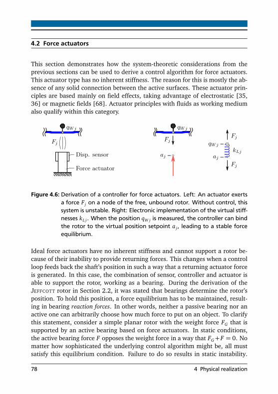
In statically determined systems, the actuator force depends on the rotor loadonly, raising the question what an active bearing can actually control. Activebearings are able to control the rotor displacements.

Active bearings with force actuators measure the shaft displacement qW andcontrol a force F and thus, from the viewpoint of control engineering, it istempting to believe that the actuator force F is the cause, while the displacementqW is the effect. From the viewpoint of structural engineering, it is clear thatthe situation is reversed. Holding the rotor in its position (cause) results inan actuator reaction force (effect). The latter statement is always compatiblewith the equilibrium conditions, while the former one is not. Although thisdifference might seem inconsequential, it alters the understanding of the forcefree condition. Going back to the considerations from Sections 3.1.1 and 3.1.3,the equations of motion for the free, unconstrained rotor are:

MqS +KRqW = −F (4.13)

Naturally, this system is unstable as the stiffness matrix KR of the free rotor isrank deficient, but active bearings can stabilize the system. When the shaft po-sition qW j is known at the j-th active bearing, a simple proportional controllerwith the gain kL j can bind the rotor to a virtual position setpoint a j using theactuator force F j . The variable names are no coincidence: the mechanical prop-erties for displacement actuators are now transferred to their controller coun-terparts. The bearing/actuator stiffness kL j is now a controller gain, and whatwas previously an actuator displacement a j is now a controller-internal virtualposition setpoint. The commanded actuator force is then F j = kL j

qW j − a j

,and using the assignments from Section 3.1.3 yields:

MqS + (KR +KL)qS = KLa+ (KR +KL)ϵ

This is the same equation that was already found in (3.23), describing a me-chanical system with force actuators. Now the same equation describes a con-trolled system that binds a rotor to the virtual position setpoint a. Special caremust be taken of the right-hand side of the equation. The unit of the expres-sion KLa is ‘force’, although it physically describes an actuator displacement ora position setpoint. Some books and publications [26, 29] substitute the ex-pression KLa with a ‘generalized force’ fa, the expression (KR +KL)ϵ with an

4.2 Force actuators 79

‘unbalance force’ fϵ, and the stiffness matrix of the supported system KR + KLwith a generalized stiffness matrix K, leading to the simplified representation:

MqS +KqS = fa + fϵ

Although these substitutions are mathematically precise, they pave the wayfor subsequent misinterpretation. A comparison between the equations of thefree rotor from Equation (4.13) contrasted with the supported one from Equa-tion (4.2), reveals that they are mathematically almost identical, although theyrepresent systems with completely different properties. The right-hand side ofEquation (4.13) represents real, physical forces, but the right-hand side of Equa-tion (4.2) are actually displacements, disguised as forces. It is in fact temptingto draw the wrong conclusion that the ’actuator forces’ fa must counteract the’unbalance forces’ fϵ so that fa+fϵ = 0. The formula’s correct interpretation getsclear when JEFFCOTT rotor’s steady state condition from Figure 2.3 is considered:the actuator displacement a must oppose the eccentricity ϵ so that the center ofmass remains in the rotational center, leading to vanishing node forces.

4.2.1 Fixed force actuators

A controller for force actuators performs two different tasks. The first and mostimportant task, is to bind the rotor to the virtual position setpoint a j so thatthe rotor is statically stabilized. The second task is the elimination of theunbalance-induced bearing forces. From the previous section it is clear thatthe stabilizing part of the controller simply resembles the displacement actua-tor stiffness electronically. Using the relation F = kL (qW − a) (The subindex jwill be omitted for improved clarity), the controller for displacement actuatorsfrom Equation (3.24) can be transformed in:

xR = (AR −BRkLCR)xR +BRkLqW

F = kL (qW −CRxR) (4.14)

The control input is the measured shaft displacement at the coordinate qW ,while the control output is the actuator force F . Although the controller wasderived from the displacement controller, their structure differs. For displace-ment controllers the system matrix was diagonal, while force controllers feature


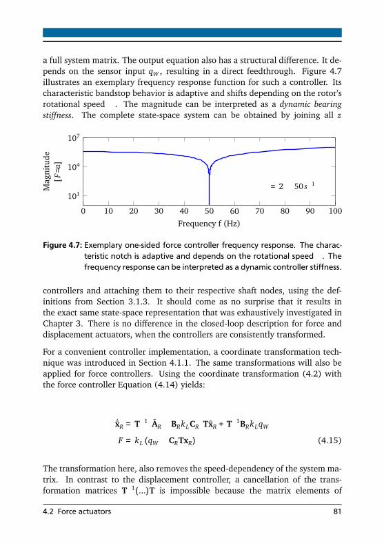
a full system matrix. The output equation also has a structural difference. It de-pends on the sensor input qW , resulting in a direct feedthrough. Figure 4.7illustrates an exemplary frequency response function for such a controller. Itscharacteristic bandstop behavior is adaptive and shifts depending on the rotor’srotational speed Ω. The magnitude can be interpreted as a dynamic bearingstiffness. The complete state-space system can be obtained by joining all z

0 10 20 30 40 50 60 70 80 90 100

101

104

107

Ω= 2π · 50 s−1

Frequency f (Hz)

Mag

nitu

de[F/a]

Figure 4.7: Exemplary one-sided force controller frequency response. The charac-teristic notch is adaptive and depends on the rotational speed Ω. Thefrequency response can be interpreted as a dynamic controller stiffness.

controllers and attaching them to their respective shaft nodes, using the def-initions from Section 3.1.3. It should come as no surprise that it results inthe exact same state-space representation that was exhaustively investigated inChapter 3. There is no difference in the closed-loop description for force anddisplacement actuators, when the controllers are consistently transformed.

For a convenient controller implementation, a coordinate transformation tech-nique was introduced in Section 4.1.1. The same transformations will also beapplied for force controllers. Using the coordinate transformation (4.2) withthe force controller Equation (4.14) yields:

˙xR = T−1

AR −BRkLCR

TxR + T−1BRkLqW

F = kL (qW −CRTxR) (4.15)

The transformation here, also removes the speed-dependency of the system ma-trix. In contrast to the displacement controller, a cancellation of the trans-formation matrices T−1(...)T is impossible because the matrix elements of

4.2 Force actuators 81

(AR − BRkLCR) are all non-zero. A forward difference discretization facilitatesa controller implementation:

xR+1 ≈ T−1

AR −BRkLCR

tS + I

TxR + T−1BRkLqW

F+1 = kL (qW −CRTxR) (4.16)

All relationships that were found for the displacement controller states xR inSection 4.1.1 are also valid for force controllers. In steady-state, the controllerstates directly represent the rotor’s eccentricity in magnitude and phase.

This section ends with some concluding remarks on controllers for force actu-ators. Figure 4.7 shows the typical notch-filter behavior for unbalance elimi-nation algorithms [42]. This behavior resulted elegantly from system-theoreticdeductions, whereas in most other works it was an a-priori choice. Even thoughmany unbalance compensation algorithms share a similar notch filter behavior,only the one presented in this work guarantees stability, as it was demonstratedin Section 2.3.4. The considerations also help to resolve the apparent contradic-tions between notch filters and adaptive feedforward compensation algorithmsmentioned in the introductory Section 1.2. In case of unconstrained rotors, thecontroller exhibits a notch filter behavior as it has to support the rotor and elimi-nate the unbalance forces. When the rotor is statically stabilized, either throughthe actuators or through an additional control loop, adaptive feedforward com-pensation can be applied. The injected harmonic signal then represents anactuator displacement which adjusts the rotational axis until all bearing forcesvanish.

4.2.2 Stiffness compensation for force actuators

Parasitic stiffnesses are not only limited to displacement actuators, but oftenmay be present when force actuators are used. According to Section 3.2.7,these stiffnesses impede the rotor’s force free operation, but may be compen-sated when they occur in the bearing plane. This is of particular interest forActive Magnetic Bearings [76]. Building on that, this section demonstrates howthe controller can be adapted in a way that also parasitic stiffnesses for forceactuators can be compensated.

The basis for the following considerations is the partitioning of the effectivebearing force F into a controllable part Fa and displacement-dependent part


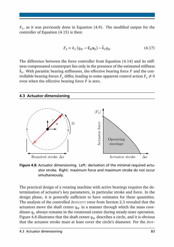
COTT rotor, the circle’s radius equals the eccentricity ϵ+, resulting in minimalabsolute actuator stroke ∆a of:

∆a ≥ 2

ϵ+

(4.18)

The steady-state actuator stroke directly depends on the rotor’s eccentricity.More than 90% of all rotors can be considered rigid [26]; in this case theInternational Standard ISO 1940 [85] provides orientation on the expected ec-centricities.

In steady-state operation, the actuator forces are zero, consequently the max-imum forces during passive rotor operation are the limiting design criterion.According to Equation (2.2), the forces are:

|FP |= k

Ω2

ω20 −Ω2

ϵ+ eiΩt

= k

Ω2

ω20 −Ω2

ϵ+

(4.19)

When the rotor’s eigenfrequencyω0 =p

m−1k is well above the rotational speedΩ, the rotor can be considered rigid. With k →∞, the equation simplifies to:

|FP |= mΩ2

ϵ+

(rigid rotor) (4.20)

Equation (4.20) allows the determination of the maximum actuator forces forrigid rotors. Together with the minimal actuator stroke from Equation (4.18),the actuator’s basic parameters are completely known. The situation is morecomplicated for flexible rotors, because according to Equation (4.19), they re-sult in theoretically unlimited forces on the bearing. For a realistic actuatordimensioning, additional assumptions are required. Either the maximum rotordisplacements are limited through the rotor casing or retainer bearings, or exter-nal damping must be assumed to limit the maximal forces and displacements.On the positive side, both forces and strokes do not occur simultaneously, asFigure 4.8 illustrates. For general rotors, the minimal required actuator strokesare a direct result of the steady-state solution (3.44):

∆aA, ...,∆az

T= 2nT

−Ω2M+ iΩ(D+G) +KR

−1KR − I

ϵ+

(4.21)

This solution is the generalization of the rotor with a single mass from Equa-tion (4.18), but in contrast to the previous solution, the required actuator dis-


placements change with the rotational speed Ω. Without damping, the actuatordisplacements become very large in the vicinity of a free rotor resonance, tend-ing to infinity. Without assuming external damping, no reasonable actuatordimensioning is possible.

Even without external damping, one can exploit the bearing invariance propertyfrom Section 3.2.8. Because the bearing’s position has no effect on the rotor’sunbalance response, they can be positioned in the vibration node of a free rotorresonance. In this case, the actuator displacements remain small even if therotor is in a free bending eigenmode.

The maximum actuator forces occur during passive rotor operation. The com-bination of Equations (3.6), (3.12), (3.16) and (3.26) results in the passivebearing forces at each bearing. Similar to its single-mass counterpart fromEquation (4.19), some damping D = 0 is required when the rotor should pass apassive, critical speed.

⎡

⎣

|FPA|...

|FPz |

⎤

⎦= nT KL

−Ω2M+ iΩ(D+G) +KR +KL

−1(KR +KL)− I

ϵ+

(4.22)

It is worth mentioning that the dimensioning guidelines only consider the forcesand strokes during steady-state operation. Naturally, the actuator requires ad-ditional strokes and forces to cover also the rotor’s transient behavior. The pre-sented equations consequently establish only lower bounds for actuator strokesand forces.

The section concludes with a summary of the derived dimensioning guide-lines:

• Maximum actuator displacements and forces are proportional to the ro-tor’s eccentricity. Without knowledge or reliable assumptions on the ro-tor’s unbalance, a useful actuator dimensioning is impossible.

• For rigid rotors, the required actuator strokes and forces can be evaluatedusing Equations (4.18) and (4.20).

• When passing a free eigenmode on a flexible rotor, additional assump-tions on the external damping are required. Alternatively, the bearingscan be placed in the nodes of the rotor’s free eigenforms.

• The maximum actuator stroke and force do not occur simultaneously.

4.3 Actuator dimensioning 85

4.4 Resonance peak avoidance

The investigated controller allows for a complete isolation of the unbalance-induced bearing forces for arbitrary rotors. In Section 3.2, it was found thata force free rotor operation close to a free resonance leads to large rotor andactuator displacements. Large rotor displacements are generally unwanted anda operation close to a free resonance should be avoided. In Section 3.10 itwas demonstrated that external mechanical damping reduces these resonances,having the drawback that a complete isolation is not possible anymore. Theremight be circumstances where external damping is unavailable or where it isnot strong enough to limit the rotor displacements in the free rotor resonances.In these cases, the controller equations can be modified to also limit the rotordisplacements in the free rotor resonances. Unfortunately, this modificationimpedes a complete force free rotor operation.

xR =

⎡

⎣

iΩ 0 00 −iΩ 00 0 −cDkD

⎤

⎦

AR

xR −

⎡

⎣

δ 0 00 δ 00 0 0

⎤

⎦

Aδ

xR +BRF (4.23)

In contrast to the previous controller, the modified version features a diagonalmatrix Aδ with two diagonal elements δ. During the controller derivation inSection 2.3.1, it was stated that the controller elements a+

F and a−B are inte-grators, defined in the their corresponding coordinate systems. In a free rotorresonance, the element a+

F is continuously integrating because there is no forceequilibrium. One can imagine the δ-element as a return spring, preventingan infinite integration. The introduction of the δ-element leads to a combina-tion of different control strategies. For δ → ∞, the integrating elements aFand aB are blocked, and the differential equation degenerates to an IntegralForce Feedback-controller [12, 30]. For δ→ 0, it returns to an ideal force freeoperation.

This additional parameter can either be determined through a simulation, or bechosen manually. In latter case, the control algorithm is initially adjusted withδ = 0. When the actuator displacements become too large, the parameter δ isincreased until the displacements remain within the limits.


5 Stability proofThe purpose of this chapter is to give a complete stability proof for the pre-viously introduced controller on arbitrary, isotropic rotors. In contrast to thedirect stability proof for the JEFFCOTT rotor demonstrated in Section 2.3.3, thecorresponding proof for general rotors is considerably more sophisticated.

The stability proof is partitioned. To begin with, a new stability theorem basedon LYAPUNOV’s stability theory is developed. This theorem is not only useful forthis particular problem, but also for general mechanical systems with attachedcollocated controllers. In a second step, the derived stability theorem is appliedto the problem of general rotors controlled by active bearings.

Some parts of this chapter are based on the work of P. C. MÜLLER, an expert inthe fields of rotordynamics [72], linear vibrations [75] and stability theory [73,74]. The particular contributions are mentioned in the corresponding section.Furthermore, the stability proof has been already published in the joint publi-cation "Unbalance and resonance elimination with active bearings on generalrotors" authored by HEINDEL, MÜLLER and RINDERKNECHT [39].

5.1 Derivation of a stability theorem

This section deals with the derivation of a LYAPUNOV stability theorem for me-chanical systems with collocated controllers. The evolution of stability theory isclosely coupled to the understanding and analysis of dynamic systems. Modernstability theory originated in 1867, when THOMSON and TAIT published Trea-tise on Natural Philosphy [56]. Back then, the stability of mechanical systemswas already well understood, including the effects of stiffness, damping andgyroscopy.

Some years later, STODOLA attempted to design a velocity governor for steamturbines, but initially failed because he could not determine the eigenvaluesof problem’s 7th-order characteristic polynomial [9]. HURWITZ then found amethod to determine stability avoiding a direct eigenvalue calculation [61]. De-spite its practicality, the proof gets tedious for systems of higher dimensions.

87

In 1892, LYAPUNOV published his work The general problem of the stability of mo-tion, which connected the problem of stability to energy considerations ratherthan eigenvalues. Using only matrix properties, it elegantly proofs stability forwhole classes of systems. Based on this idea, researches have obtained remark-able stability theorems within the last century, including ones for complicatedmechanical arrangements [7, 48].

However, the special matrix structure of mechanical systems with collocatedcontrollers inhibits a treatment of the problem using LYAPUNOV’s stability the-ory [74]. Although INMAN proves stability for collocated controllers, his as-sumed matrix structure represents a standard mechanical system and is lackingin continuing progress over established solutions [49].

The absence of available solutions encouraged the development of a new the-orem for mechanical systems with collocated controllers. After an introductionto the fundamentals of LYAPUNOV stability, the characteristic matrix structure ofcollocated systems is explained with a simple example. After the derivation ofa stability theorem for this system, the approach is generalized to systems ofarbitrary dimensions. Finally, the solution is extended to mechanical systemswith damping and gyroscopy.

5.1.1 Fundamentals of Lyapunov stability

Figure 5.1: Three mass oscillator with damping.

An introductory example demonstrates how quickly a stability analysis basedon HURWITZ-determinants leads to complicated calculations even for a simplesystems. Figure 5.1 depicts an oscillatory, damped system with three massesand the corresponding equation of motion:

Mq+Dq+Kq = 0 (5.1)

88 5 Stability proof

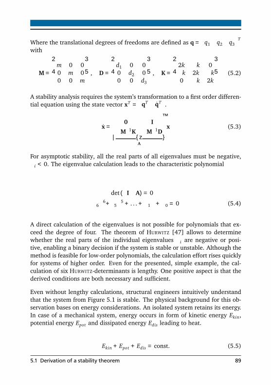
Where the translational degrees of freedoms are defined as q =

q1 q2 q3

T

with

M =

⎡

⎣

m 0 00 m 00 0 m

⎤

⎦ , D =

⎡

⎣

d1 0 00 d2 00 0 d3

⎤

⎦ , K =

⎡

⎣

2k −k 0−k 2k −k0 −k 2k

⎤

⎦ (5.2)

A stability analysis requires the system’s transformation to a first order differen-tial equation using the state vector xT =

qT qT

.

x =

0 I

−M−1K −M−1D

A

x (5.3)

For asymptotic stability, all the real parts of all eigenvalues must be negative,λi < 0. The eigenvalue calculation leads to the characteristic polynomial

det (λI−A) = 0

α6λ6+α5λ

5 + . . .+α1λ+α0 = 0 (5.4)

A direct calculation of the eigenvalues is not possible for polynomials that ex-ceed the degree of four. The theorem of HURWITZ [47] allows to determinewhether the real parts of the individual eigenvalues λi are negative or posi-tive, enabling a binary decision if the system is stable or unstable. Although themethod is feasible for low-order polynomials, the calculation effort rises quicklyfor systems of higher order. Even for the presented, simple example, the cal-culation of six HURWITZ-determinants is lengthy. One positive aspect is that thederived conditions are both necessary and sufficient.

Even without lengthy calculations, structural engineers intuitively understandthat the system from Figure 5.1 is stable. The physical background for this ob-servation bases on energy considerations. An isolated system retains its energy.In case of a mechanical system, energy occurs in form of kinetic energy Ekin,potential energy Epot and dissipated energy Edis leading to heat.

Ekin + Epot + Edis = const. (5.5)

5.1 Derivation of a stability theorem 89

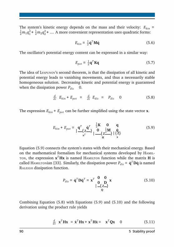
The system’s kinetic energy depends on the mass and their velocity: Ekin =12 m1q2

1 +12 m2q2

2 + .... A more convenient representation uses quadratic forms:

Ekin =12 qT Mq (5.6)

The oscillator’s potential energy content can be expressed in a similar way:

Epot =12 qT Kq (5.7)

The idea of LYAPUNOV’s second theorem, is that the dissipation of all kinetic andpotential energy leads to vanishing movements, and thus a necessarily stablehomogeneous solution. Decreasing kinetic and potential energy is guaranteedwhen the dissipation power Pdis ≥ 0.

dd t

Ekin + Epot

= − dd t

Edis

= −Pdis ≤ 0 (5.8)

The expression Ekin + Epot can be further simplified using the state vector x.

Ekin + Epot =

qT qT

xT

12 K 00 1

2 M

H

qq

x

(5.9)

Equation (5.9) connects the system’s states with their mechanical energy. Basedon the mathematical formalism for mechanical systems developed by HAMIL-TON, the expression xT Hx is named HAMILTON function while the matrix H iscalled HAMILTONian [33]. Similarly, the dissipation power Pdis = qT Dq is namedRALEIGH dissipation function.

Pdis = qT DqT = xT

0 00 D

Q

x (5.10)

Combining Equation (5.8) with Equations (5.9) and (5.10) and the followingderivation using the product rule yields

dd t

xT Hx

= xT Hx+ xT Hx = −xT Qx≤ 0 (5.11)


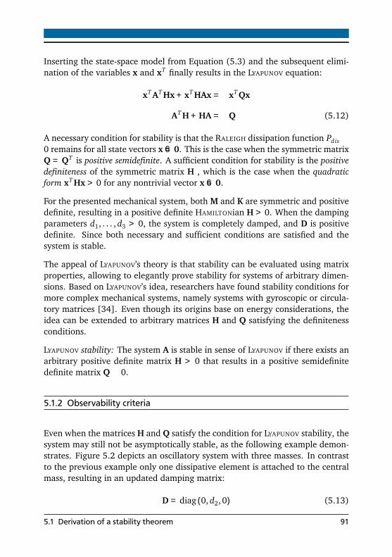
Inserting the state-space model from Equation (5.3) and the subsequent elimi-nation of the variables x and xT finally results in the LYAPUNOV equation:

xT AT Hx+ xT HAx = −xT Qx

AT H+HA = −Q (5.12)

A necessary condition for stability is that the RALEIGH dissipation function Pdis ≥0 remains for all state vectors x = 0. This is the case when the symmetric matrixQ = QT is positive semidefinite. A sufficient condition for stability is the positivedefiniteness of the symmetric matrix H , which is the case when the quadraticform xT Hx> 0 for any nontrivial vector x = 0.

For the presented mechanical system, both M and K are symmetric and positivedefinite, resulting in a positive definite HAMILTONian H> 0. When the dampingparameters d1, . . . , d3 > 0, the system is completely damped, and D is positivedefinite. Since both necessary and sufficient conditions are satisfied and thesystem is stable.

The appeal of LYAPUNOV’s theory is that stability can be evaluated using matrixproperties, allowing to elegantly prove stability for systems of arbitrary dimen-sions. Based on LYAPUNOV’s idea, researchers have found stability conditions formore complex mechanical systems, namely systems with gyroscopic or circula-tory matrices [34]. Even though its origins base on energy considerations, theidea can be extended to arbitrary matrices H and Q satisfying the definitenessconditions.

LYAPUNOV stability: The system A is stable in sense of LYAPUNOV if there exists anarbitrary positive definite matrix H > 0 that results in a positive semidefinitedefinite matrix Q≥ 0.

5.1.2 Observability criteria

Even when the matrices H and Q satisfy the condition for LYAPUNOV stability, thesystem may still not be asymptotically stable, as the following example demon-strates. Figure 5.2 depicts an oscillatory system with three masses. In contrastto the previous example only one dissipative element is attached to the centralmass, resulting in an updated damping matrix:

D = diag (0, d2, 0) (5.13)


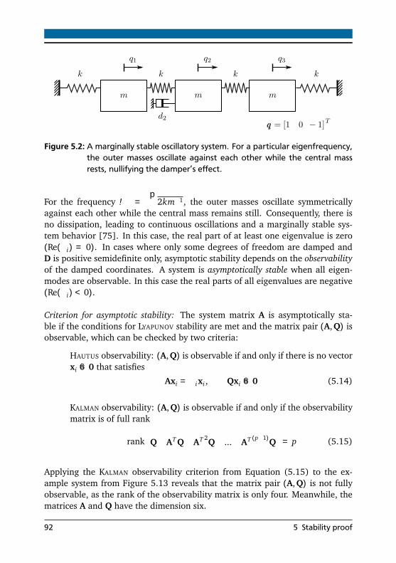
masses which is depicted in figure ??.

Figure 5.2: A marginally stable oscillatory system. For a particular eigenfrequency,the outer masses oscillate against each other while the central massrests, nullifying the damper’s effect.

For the frequency ω =p

2km−1, the outer masses oscillate symmetricallyagainst each other while the central mass remains still. Consequently, there isno dissipation, leading to continuous oscillations and a marginally stable sys-tem behavior [75]. In this case, the real part of at least one eigenvalue is zero(Re(λi) = 0). In cases where only some degrees of freedom are damped andD is positive semidefinite only, asymptotic stability depends on the observabilityof the damped coordinates. A system is asymptotically stable when all eigen-modes are observable. In this case the real parts of all eigenvalues are negative(Re(λi)< 0).

Criterion for asymptotic stability: The system matrix A is asymptotically sta-ble if the conditions for LYAPUNOV stability are met and the matrix pair (A,Q) isobservable, which can be checked by two criteria:

HAUTUS observability: (A,Q) is observable if and only if there is no vectorxi = 0 that satisfies

Axi = λixi , Qxi = 0 (5.14)

KALMAN observability: (A,Q) is observable if and only if the observabilitymatrix is of full rank

rank

Q AT Q AT 2Q ... AT (p−1)Q

= p (5.15)

Applying the KALMAN observability criterion from Equation (5.15) to the ex-ample system from Figure 5.13 reveals that the matrix pair (A,Q) is not fullyobservable, as the rank of the observability matrix is only four. Meanwhile, thematrices A and Q have the dimension six.


Even when systems are not completely damped, they can be asymptoticallystable. The example considered is now modified in such a way that thedamper is attached to the coordinate q1, the damping matrix changes toD = diag (d1, 0, 0). In this case, the matrix pair (A,Q) is fully observable andtherefore asymptotically stable. Systems where damping affects only some de-grees of freedom (D ≥ 0), but which are still asymptotically stable are calledpervasively damped [84, 99]. This case is of particular interest for rotating ma-chinery, where in many cases significant damping is only provided through thebearings.

5.1.3 A simple system with semidefinite mass matrix

Figure 5.3: A damped mechanical system with a massless guide. The application ofLyapunov’s theory is difficult for systems with semidefinite mass matri-ces.

Throughout the last century, stability theorems have been found even for com-plex mechanical systems. On the other hand, there are even simple systemswhere LYAPUNOV’s theory cannot be applied. The mechanical system from Fig-ure 5.3 represents such an example. The corresponding matrices are:

M =

m 00 0

, D =

0 00 c−1

D

, K =

k1 −k1

−k1 k1 + kD

. (5.16)

Since the mass matrix M is positive semidefinite and consequently noninvert-ible, the state-space representation from Equation (5.3) is invalid. With themodified state vector xT =

q1 q1 aD

T, the system matrix yields

A =

⎡

⎣

0 1 0−m−1k1 0 m−1k1

cDk1 0 −cD (k1 + kD)

⎤

⎦ (5.17)


Since the matrix structure of A has changed, the HAMILTONian found in Equa-tion (5.9) does not satisfy the LYAPUNOV equation, partly because of a dimen-sional mismatch, but mainly because the state vector x lacks the state aD whichis needed for the dissipation function xT Qx. Finding a suitable HAMILTONianfor mechanical systems with semidefinite mass matrices M ≥ 0 has been underinvestigation by various researchers [27, 74, 96]. Instead of finding a suitableHAMILTONian H for the modified system, the presented works rely on proofsby contradiction. On the downside, these approaches forfeit the elegance andclearness of the initial LYAPUNOV proof.

Although LYAPUNOV’s theory originated from energy considerations, it can befurther generalized. Any arbitrary matrix H > 0 that results in a positivesemidefinite matrix Q≥ 0 implies a stable system matrix A. Theoretically, thesematrices could be chosen arbitrarily, but their definiteness properties must beknown. Since the definiteness of a matrix depends on its eigenvalues, the prob-lem shifts from the eigenvalue calculation of A to the eigenvalues of H and Q.Consequently, this helps only when the matrices have a structure that allows fora simple determination of the definiteness properties. When the matrices arediagonal or block-diagonal, determining the definiteness is relatively easy, as itonly depends on the diagonal elements. For instance, the matrices from Equa-tions (5.9) and (5.10) have such a convenient form, that results in an elegantstability proof for M,D,K-systems. Unfortunately, there is no general recipe howto choose the matrices H and Q so that they count with favorable properties. Asstarting point for good choices of the matrix Q is the inclusion of dissipation ele-ments at their respective coordinates, as it was done in Equation (5.10). For thesystem of Figure 5.3, the dissipation function is Pdis = aDc−1

D aD. Since only theposition aD is part of the state vector x, a direct dissipation representation withrespect to aD is not possible and the quantity aD2c−1

D aD is chosen instead.

Q = diag

0, 0,2c−1D

(5.18)

The expression is physically meaningless, but the symmetric and positivesemidefinite matrix Q serves as valid starting point for the solution of Equa-tion (5.12). With both A and Q defined, the solution H can be determined.

Historically, several methods for the analytical solution of LYAPUNOV equationsemerged. One method bases on LEVERRIER-FADDEEV-matrices [73, 74], anothermethod bases on the KRONECKER-product [8, 17]. Latter method defines a (p×p)matrix H with the unknowns h11...hpp. Expanding the LYAPUNOV equation leadsto a system of p2 linear equations, which can be solved with standard methods.


The complexity is further reduced since H = HT , so only the upper triangularmatrix must be considered, reducing the number of unknowns to p (p− 1)/2.

Due to the large number of equations, the manual calculation of analytical solu-tions is complicated and prone to errors. Using computer algebra systems suchas Mathematica or Matlab solve even complicated analytical problems almostinstantly and without errors. The following result was obtained using MATLAB’ssymbolic toolbox.

H =

⎡

⎣

m 0 00 m2 k−1 mc−1

D k−1D

0 mc−1D k−1

D c−2D k−1

D

⎤

⎦ with k−1 =k1 + kD

k1kD(5.19)

The matrix is positive definite if the leading principal minors are positive [3].

a1 = m

a2 =

m 00 m2 k

= m3 k

a3 =

m 0 00 m2 k−1 mc−1

D k−1D

0 mc−1D k−1

D c−2D k−1

D

= m3c−2D (k1kD)

−1

The matrix is positive definite when the mass m is positive, the series connectionof the two stiffnesses is positive k > 0 and the product k1kD is positive. It issurprising that an arbitrary value for cD leads to H > 0, however Q is positivedefinite only for cD > 0. To summarize, a sufficient condition for the stabilityof A is that the parameters m, k1, kD, cD are positive. This result is consistentwith the expectations of a mechanical engineer. Indeed, the same result can beobtained with less effort using the HURWITZ stability criterion [9, 47]. However,the advantages of LYAPUNOV’s theory are better visible for large systems.

5.1.4 Complex mechanical systems

The previous section demonstrated how a suitable HAMILTONian for a simplemechanical system with a semidefinite mass matrix can be found. This basicstability proof is now extended to a more complex mechanical system. Howeverit is modified in such a way that preserves various similarities with the previousresult.


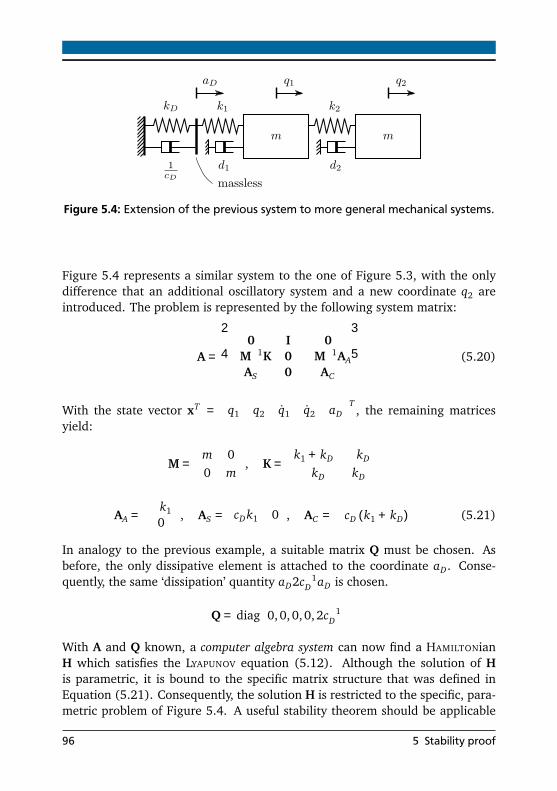
Figure 5.4: Extension of the previous system to more general mechanical systems.

Figure 5.4 represents a similar system to the one of Figure 5.3, with the onlydifference that an additional oscillatory system and a new coordinate q2 areintroduced. The problem is represented by the following system matrix:

A =

⎡

⎣

0 I 0−M−1K 0 −M−1AA

AS 0 AC

⎤

⎦ (5.20)

With the state vector xT =

q1 q2 q1 q2 aD

T, the remaining matrices

yield:

M =

m 00 m

, K =

k1 + kD −kD

−kD kD

AA =

−k10

, AS =

cDk1 0

, AC = −cD (k1 + kD) (5.21)

In analogy to the previous example, a suitable matrix Q must be chosen. Asbefore, the only dissipative element is attached to the coordinate aD. Conse-quently, the same ‘dissipation’ quantity aD2c−1

D aD is chosen.

Q = diag

0,0, 0, 0, 2c−1D

With A and Q known, a computer algebra system can now find a HAMILTONianH which satisfies the LYAPUNOV equation (5.12). Although the solution of His parametric, it is bound to the specific matrix structure that was defined inEquation (5.21). Consequently, the solution H is restricted to the specific, para-metric problem of Figure 5.4. A useful stability theorem should be applicable


for more general systems such as the one from Equation (5.20) – with only fewrestrictions on the structure of M,K,AA,AS ,AC .

It would appear that finding a general HAMILTONian for Equation (5.20) shouldbe manageable, considering that it inherits the same matrix structure as thesimple system of Equation (5.17) where a solution was easily found. Unfortu-nately, the block-matrix structure of Equation (5.20) inhibits the use of directsolution techniques that were introduced in Section 5.1.3. Contrary to scalarcalculations, matrix algebra is not commutative, so X·Y is generally not the sameas Y · X. Even though some computer algebra systems support noncommutativematrix algebra, a different solution technique is preferred.

The presented approach has the advantage of not requiring noncommutativematrix algebra. It bases on the hypothesis that there is a solution H for the gen-eral state-space system A of Equation (5.20) which can be expressed somehowin terms of the matrices M,K,AA,AS ,AC . If this hypothesis holds, the HAMIL-TONian of Equation (5.19) must be a specific solution for the still unknown,general matrix H. Similarly, if there is a universal solution for H, inserting thespecific matrices of Equation (5.21) must result in the correct solution of theLYAPUNOV equation. Any specific system must be a part of the general solution.This property can be exploited to find a general solution:

• Create the simplest (scalar) system A that satisfies the problem’s generalmatrix structure (In this case, Equation (5.17) is the simplest system thatsatisfies the general form of Equation (5.20)).

• Set-up a matrix Q and find a parametric solution H with a computer usingthe techniques presented in Section 5.1.3.

• Express the scalar solution matrix H in terms of the matrices M,K,AA, ...

• Create a new, more complex system matrix A. (The matrices of Equa-tion (5.1.4) are a good choice to proceed).

• Find a parametric solution H using the computer. Check if the guessedmatrix operation still satisfies the more complex system. Modify if neces-sary.

• The process is finished when the guessed solution for H automaticallysatisfies any new system.

• The final solution is verified using the LYAPUNOV equation.


The presented process is highly iterative and certainly lacks the mathematicalelegance of a direct calculation. On the other hand, it is unclear if there evenare efficient methods to solve the LYAPUNOV equation when only the generalblock-matrix structure and their respective matrix properties are known. Thepresented method demonstrates a straightforward way to obtain a stability the-orem for a collocated mechanical system, and should be seen only as a tool. Infuture works, this manual approach could be replaced by dedicated algorithmsto find stability theorems for even more complex systems.

5.1.5 Damping, gyroscopy and complexity

To generalize the result of the previous section further, the system can be aug-mented with a damping matrix D and a gyroscopic matrix G. Similar to thematrices M and K, the damping matrix D = DT is symmetric, whereas the gyro-scopic matrix G = −GT is skew-symmetric.

A =

⎡

⎣

0 I 0−M−1K −M−1 (D+G) −M−1AA

AS 0 AC

⎤

⎦ (5.22)

Equation (5.22) augments the previous system from Equation (5.4) with damp-ing and gyroscopy. The introduction of a dissipative matrix D also requires anupdate of Q. In Equation (5.10), the quadratic form Pdis = qT Dq representedthe dissipation energy. With the state-space vector xT =

q q xR

T, the nat-

ural choice for Q = diag (0, 2D, ...), representing a dissipation energy. However,it turns out that solutions of H become large and cumbersome. The alterna-tive choice Q = diag (2D,0, ...) results in simpler solutions H. Even thoughthe quantity is physically meaningless, the definiteness properties of Q remainunaffected.

Gyroscopic forces are conservative and do not alter the system’s energy [34].For this reason, the gyroscopic matrix G does not contribute to the dissipationfunction, leaving the dissipation matrix Q unchanged. The augmented systemwith the previously presented techniques.

So far, it is supposed that the matrix A is real. The use of complex coordinatesrequires an extension of the stability theorem to complex numbers. The com-


plex version of the LYAPUNOV Equation (5.12) is similar to the real one [21],except that it requires the complex conjugate transpose AH :

AHH+HA = −Q (5.23)

The introduction of complex coordinates leads to updated symmetry properties:the matrix D = DH must be hermitian, and the matrix G = −GH is now skew-hermitian. Permitting complex matrices A may lead to problems with somecomputer algebra systems. As a solution, each complex matrix can be decom-posed into a real (subindex “r”), and an imaginary (subindex “i”) part, leadingto two individual problems with real coefficient matrices.

(Ar + iAi)H

AH

(Hr + iHi)

H

+(Hr + iHi)

H

(Ar + iAi)

A

= − (Qr + iQi)

Q

(5.24)

real: ATr Hr +HrAr +AT

i Hi −HiAi = −Qr (5.25)

imag: ATr Hi +HiAr −AT

r Hr +HrAi = −Qi!= 0 (5.26)

5.1.6 Lyapunov stability theorem for controlled mechanical systems

The previous considerations result in a LYAPUNOV stability theorem for generalmechanical systems with collocated controllers. This result has already beenpublished in a publication written bei HEINDEL, MÜLLER and RINDERKNECHT [39].Consider a matrix A of the structure

A =

⎡

⎣

0 I 0−M−1K −M−1(G+D) −M−1AA

AS 0 AC

⎤

⎦ (5.27)

with hermitian matrices M,K,D and a skew-hermitian matrix G. It is furtherassumed that an arbitrary chosen matrix P with the following properties can befound:

• P satisfies AHA = PAS (generalized collocation),

• The matrix product PAC is hermitian, i.e. PAC = (PAC)H .


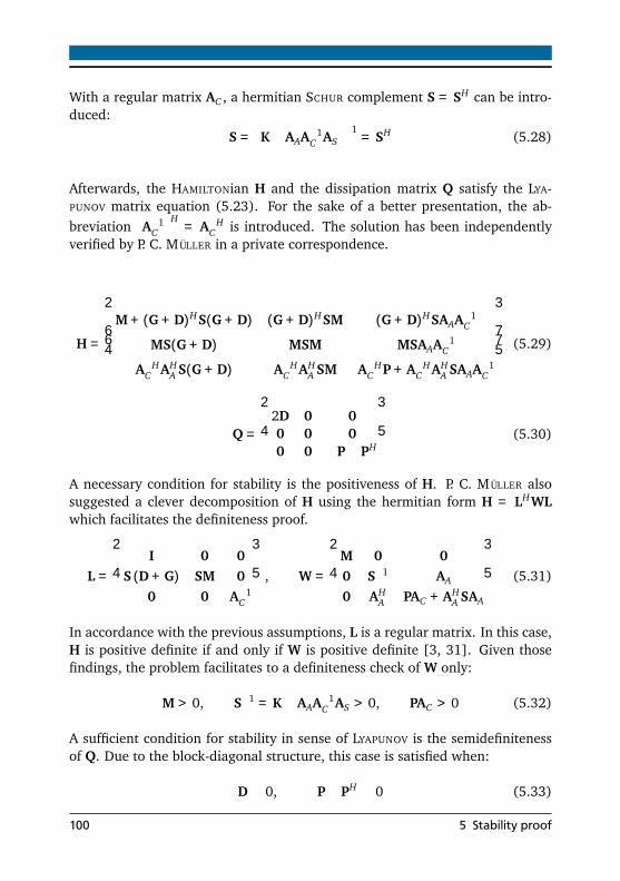
With a regular matrix AC , a hermitian SCHUR complement S = SH can be intro-duced:

S =

K−AAA−1C AS

−1= SH (5.28)

Afterwards, the HAMILTONian H and the dissipation matrix Q satisfy the LYA-PUNOV matrix equation (5.23). For the sake of a better presentation, the ab-breviation

A−1C

H= A−H

C is introduced. The solution has been independentlyverified by P. C. MÜLLER in a private correspondence.

H =

⎡

⎢

⎢

⎣

M+ (G+D)HS(G+D) (G+D)HSM (G+D)HSAAA−1C

MS(G+D) MSM MSAAA−1C

A−HC AH

A S(G+D) A−HC AH

A SM A−HC P+A−H

C AHA SAAA−1

C

⎤

⎥

⎥

⎦

(5.29)

Q =

⎡

⎣

2D 0 00 0 00 0 −P− PH

⎤

⎦ (5.30)

A necessary condition for stability is the positiveness of H. P. C. MÜLLER alsosuggested a clever decomposition of H using the hermitian form H = LHWLwhich facilitates the definiteness proof.

L =

⎡

⎣

I 0 0S (D+G) SM 0

0 0 A−1C

⎤

⎦ , W =

⎡

⎣

M 0 00 S−1 AA

0 AHA PAC +AH

A SAA

⎤

⎦ (5.31)

In accordance with the previous assumptions, L is a regular matrix. In this case,H is positive definite if and only if W is positive definite [3, 31]. Given thosefindings, the problem facilitates to a definiteness check of W only:

M> 0, S−1 = K−AAA−1C AS > 0, PAC > 0 (5.32)

A sufficient condition for stability in sense of LYAPUNOV is the semidefinitenessof Q. Due to the block-diagonal structure, this case is satisfied when:

D≥ 0, −P− PH ≥ 0 (5.33)


As a concluding remark, it shall be noted that the conditions (5.32), (5.33)only guarantee marginal stability, that is Re(λi) ≤ 0, since Q is semidefinite.Asymptotic stability can be proven with the observability criterion from Sec-tion 5.1.2.

5.1.7 A note on circulatory matrices and inner damping

Most mechanical systems can be represented with mass, stiffness, damping andgyroscopic matrices. However, some systems count with forces whose defini-tion depends on the displacement of the body on which they act, so calledfollower forces [44]. Due to their nonconservative nature, they differ fromthe conservative elastic forces and cannot be represented in a stiffness matrix.The position-dependent, but skew-symmetric circulatory matrix N = −NH rep-resents these forces [49]. For example, an aeroelastic instability phenomenoncalled flutter is contributed to follower forces [41]. On aircraft, flutter causesvibrations of the wings or control surfaces and may lead to structural damage[95].

In rotordynamics, circulatory matrices are mainly attributed to inner damping.As already mentioned in Section 3.2.5, it describes damping that occurs on therotor itself. This phenomenon is of particular interest as it may lead to violentvibrations [94]. This effect often occurs on built-up rotors which are assembledfrom several force- or form-fitted elements, such as discs or blades [63]. It isfound that this instability mechanism is mathematically closely related to flutter,as the damping’s coordinate transformation from rotating to inertial coordinatesalso leads to skew-symmetric matrices N. It is worth mentioning that innerdamping is ambivalent: for subcritical rotor operation, it stabilizes the rotor,whereas it destabilizes the system for supercritical operation [28].

Finding stability theorems for systems with circulatory forces is difficult, asthe nonconservative nature of N makes it difficult to find suitable LYAPUNOV-functions [34]. MINGORI distinguished between systems with actual followerforces and those where circulatory matrices arise only in certain coordinatesystems [69, 70]. For the latter ones, he demonstrates that an appropriate coor-dinate transformation eliminates the circulatory matrices, and that the resultingsystem can be processed using standard methods. The proposed transformationonly worked for positive definite damping matrices D > 0, a restriction whichcould be dropped in a consecutive work [74].

Attempts to widen the presented stability proof to systems with circulatoryforces were unsuccessful. Using the method from Section 5.1.4 resulted in


overly complex solutions for the HAMILTONian H even for simple systems, beingtoo complicated to be useful. When general stability statements are required,an adaption of MINGORI’s transformation theorem to controlled mechanical sys-tems is promising. For the investigation of a particular machine, a numericeigenvalue calculation is the fastest way to check stability.

5.2 Stability of the controlled rotor

The stability theorem is now used to prove the stability of the controlled systemwith arbitrary rotors. To enhance readability, the proof is sectioned. Startingwith the proof’s applicability, the reasoning shifts to a check of the matrix def-initeness properties. A subsequent proof of the system’s observability ensuresasymptotic stability. In conclusion, all necessary and sufficient conditions forstability are conveniently listed.

5.2.1 Proof applicability

A prerequisite for the stability proof is the checking of whether or not the prooffor collocated mechanical systems from Equation (5.27) is applicable to the sys-tem matrix of the controlled rotor system from Equations (3.27) and (3.40).The presented proof was tailored to the problem and later generalized. Conse-quently it is no surprise that the system matrix of the controlled rotor indeedsatisfies the conditions. A matrix comparison reveals that:

K = KR +KL (5.34)

And for the controller Equations:

AA = −KLnCR, AS = BRnT KL , AC = AR −BRnT KLnCR (5.35)

According to the conditions of Section 5.1.6, the stability proof is only appli-cable if an arbitrary matrix P can be found which satisfies both the conditionsfor generalized collocation, and also the condition that the matrix product PACmust be hermitian. With P defined as:


P = diag

PA,PB, · · · ,P j , · · ·

, P j =

⎡

⎣

−i c−1C j 0 0

0 i c−1C j 0

0 0 −c−1D j

⎤

⎦ (5.36)

The condition for generalized collocation requires that AHA = PAS . Using the

relations from Equation (5.35) and (5.36), the problem can be rewritten asCH

R = −PBR. The block-diagonal, repetitive form of the matrices BR, CR of Equa-tion (3.25) reduces the problem to only one block, and results in the conditionbeing satisfied. Furthermore, the condition PAC = (PAC)H must be satisfied andcan be rewritten as PAC = PAR + (nCR)

T KLnCR. As it turns out, the secondsummand is a hermitian form, so only the first summand PAR must be checked.This is true since the resulting matrix is diagonal and real. With both conditionssatisfied, it is clear that Equation (5.36) is valid and the proof is applicable.

5.2.2 Positive definiteness of H

A necessary condition for the stability of the matrix A is the positive definitenessof H. According to Equation (5.32), the first condition is that M> 0. A semidef-inite mass matrix can be ruled out as Equation (5.27) requires its inverse. Thus,M must be regular. A second condition is that the inverse SCHUR complementS−1 = K−AAA−1

C AS is positive definite:

S−1 = K−AAA−1C AS = KR +KL +KLnCR

AR −BRnT KLnCR

−1BRnT KL (5.37)

The WOODBURY Matrix Identity [40, 97] could be applied to simplify the expres-sion, but it requires the regularity of KL , which is generally not given. Theproblem is solved by expanding the expression KL = KLnnT = nnT KL , as theexpression nnT acts like a neutral element for KL . Finally, the matrix nT KLn isper definition invertible, and Equation (5.37) can first be rewritten and subse-quently simplified:

S−1 = KR + n

nT KLn+ nT KLnCR

AR −BRnT KLnCR

−1BRnT KLn

nT

= KR + n

nT KLn−1 −CRA−1

R BR

−1nT

= KR + ndiag

· · · , k−1L j + k−1

D j + 2cC jΩ−1, · · ·

−1nT for any j (5.38)

5.2 Stability of the controlled rotor 103

Two conditions govern the definiteness of the inverse SCHUR complement S−1

from Equation (5.38). The first summand is the positive semidefinite rotor stiff-ness matrix KR. The second summand is at least positive semidefinite when itsinner diagonal matrix is positive definite. A sufficient condition is that the sum-mands kL j , kD j , and 2cC jΩ

−1 are all positive. It is remarkable that the parameter2cC jΩ

−1 might lead to instability for negative values of Ω. This surprising re-sult was already found during the stability analysis of the controlled JEFFCOTT

rotor in Section 2.3.3. As a solution, a new parameter cC j from Equation (2.27)was introduced to circumvent the problem. Finally, the sum of both semidefi-nite summands KR + ndiag (· · · )−1 nT must be positive definite, which is givenwhen KR +KL > 0. This condition means that the rotor must be supported in astatically (in-)determined manner by the bearings.

The last condition for H> 0 is the positive definiteness of PAC . In Section 5.2.1the relation PAC = PAR + (nCR)

T KLnCR was uncovered. The second summandis at least positive semidefinite, consequently the first one must be positive def-inite. The block-diagonal form of both P and AR reduces the definiteness checkto a check of the definiteness of P jARj .

P jARj = diag

c−1C j Ω, c−1

C j Ω, kD j

= diag

c−1C j , c−1

C j , kD j

(5.39)

Equation (5.39) is positive definite when all parameters kD j and cC j are positivefor each controller j. This condition is redundant to the ones found earlier.After all conditions have been satisfied, it is clear that H> 0.

5.2.3 Positive semidefiniteness of Q

According to Equation (5.33), Q is positive semidefinite when either the me-chanical damping matrix is positive semidefinite D≥ 0 or when the matrix sum−P−PH is positive semidefinite. Using the definition of P from Equation (5.36)yields:

− P− PH = diag

...,−P j − PHj , ...

, −P j − PHj = diag

0, 0, 2c−1D j

(5.40)

The expression is positive semidefinite when the controller parameters cD j arepositive. An external mechanical damping D is not required to ensure positivesemidefiniteness of Q.


5.2.4 Observability and asymptotic stability

The previous section proved that the system matrix A of the controlled rotor isat least stable in sense of LYAPUNOV, hence at least marginally stable. However,a successful control requires asymptotic stability. Section 5.1.2 stated that anadditional stability criterion must be satisfied to guarantee asymptotic stability.In this case, the HAUTUS-criterion is used. The matrix pair (A,Q) is completelyobservable if and only if there does not exist an eigenvector xi of A which isorthogonal to Q:

(A−λiI)xi = 0, Qxi = 0 for all i (5.41)

Together with the definition of the matrix A from Equation (3.44) and Q fromEquation (5.30), this observability definition leads to the following expres-sions:

Mλ2i + (D+G)λi +K

qSi +AAxRi = 0, DqSi = 0 (5.42)

ASqSi + (AC −λiI)xRi = 0,

P+ PH

xRi = 0 (5.43)

The stability criterion of Equations (5.42) and (5.43) can be divided into twodifferent cases, which will be treated separately:

Case I: Pervasive damping. When assuming that the controller states are zero,hence xRi = 0, the reduced equations are:

Mλ2i +Gλi +K

qSi = 0, ASqSi = 0, DqSi = ? (5.44)

This case can also be divided in two cases. The first case is that the passivemechanical system without controller is pervasively damped:

rank

Mλ2i + (D+G)λi +K

Dλi

= p for all λi (5.45)


Equation (5.45) is an observability criterion for the mechanical subsystem,where p reflects the number of shaft nodes. When this condition is satisfied,it is guaranteed that DqSi = 0, and the system is pervasively damped and con-sequently asymptotically stable. In case that the mechanical damping is notpervasive, there is at least one i with λi , qSi = 0, so that

Mλ2i + (D+G)λi +K

qSi = 0, DqSi = 0 (5.46)

Now asymptotic stability depends on the expression ASqSi:

ASqSi = BRnT KLqSi = BRnT KLn

rank=z

nT qSi

−→ ASqSi = 0 ⇐⇒ nT qSi = 0 (5.47)

The system is marginally stable when the natural vibrations of the passive me-chanical systems have vibration nodes at all bearings. When for at least at onebearing nT

j qSi = 0, hence at least one bearing is not located in the vibrationnode, damping is introduced through this bearing and the controlled system isasymptotically stable.

Case II: Free rotor resonance. In this case, it is assumed that xRi = 0, but

P+ PH

xRi = 0. This is only possible when all controller damping elementsare zero, hence aD ji = 0 for all controllers. According to the controller Equa-tion (3.24), this also leads to vanishing forces at all bearings, hence F j = 0.The controller equation then simplifies to xRj = ARjxRj . For λi = ±iΩ, there arenontrivial eigenvectors xRj+ and xRj− that solve the following equation:

For λi = +iΩ :

ARj − iΩI

xRj+ = 0 with xRj+ =

1 0 0T

(5.48)

For λi = −iΩ :

ARj + iΩI

xRj− = 0 with xRj− =

0 1 0T

(5.49)

With these particular eigenvalues λi = ±iΩ, the eigenvalue problem from Equa-tion (5.43) with the matrix definitions from Equation (5.35) leads to:


ASqSi + (AC −λiI)xRi = 0 for λi = ±iΩ

BRnT KLqSi +

AR ± iΩI

xRi

=0

−BRnT KLnCRxRi = 0 (5.50)

Using the definition that relates the controller states xRi with the actuator dis-placements ai from Equations (3.21) and (3.25) gives:

BRnT KLqSi −BRnT KL nCRxRi

ai

= 0

BRnT KL

reg.

(qSi − ai) = 0

qSi = ai (5.51)

With this result, the mechanical subsystem from Equation (5.42) is consid-ered:

Mλ2i + (D+G)λi +K

qSi +AAxRi = 0 (5.52)

With the matrix definitions from Equations (5.34), (5.35) and the result fromEquation (5.51) finally leads to:

−MΩ2 ± iΩ (D+G) +KR +KL

qSi −KL nCRxRi

=ai=qSi

= 0

−MΩ2 ± iΩ (D+G) +KR

qSi = 0 (5.53)

The problem now reduces to an investigation of the mechanical system: If thereis a nontrivial eigenvector qSi = 0 that solves Equation (5.53), the system ismarginally stable only. On the contrary, if qSi = 0 is the only solution, the sys-tem is asymptotically stable. The mechanical interpretation of Equation (5.53)is the following: The equation represents the free, unconstrained rotor. A non-trivial eigenvector qSi exists when the rotational speed Ω matches a free rotorresonance (λi = +iΩ is the forward whirl; whereas λi = −iΩ is the backwardwhirl). When no external mechanical damping is present DqSi = 0, the systemis only marginally stable in the free rotor resonance.


5.2.5 Proof results

The diversity of different conditions complicate the stability proof. Removingthe redundant conditions and categorizing them leads to a few comprehensibleresults:

• Mechanical system:The mass matrix must be positive definite. (M> 0)The stiffness matrix of the free rotor is positive semidefinite. (KR ≥ 0)The rotor is entirely supported by the active bearings. (KR +KL > 0)Mechanical damping may or may not be present. (D≥ 0)The system is stable in presence of gyroscopy. (G = −GH)The proof gives no statements for circulatory matrices (N = 0)

• Controller:All controller stiffness parameters are positive. (kL j , kD j > 0)The controller damping parameters are positive. (cD j > 0)The controllers adaption parameters are positive. (cC j > 0)

• Asymptotic stability:Is given when the external mechanical damping is pervasive. (DqSi = 0)Without external mechanical damping (D = 0):

– Is given when the rotational speed Ω does not match the rotor’sfree eigenfrequency (Ω2 +λ2

i = 0)

– At least one bearing must be outside the rotor’s passive vibrationnodes (nT qSi = 0)


6 ExperimentsA series of experiments is performed to evaluate whether the previous assump-tions hold under real-world conditions. Two test rigs with different rotor con-figurations are used to compare the theoretic considerations with the experi-mental results. Both test rigs are equipped with piezoelectric actuators as activeelements.

6.1 Rotor with one disc and piezoelectric actuators

Figure 6.1: Jeffcott rotor test rig with one disc and one active bearing. Left: theactive bearing assembly with piezoactuators and collocated force sen-sors displaces the shaft, while the coil springs ensure the mechanicalintegrity. Right: Displacement sensors measure the disc’s position, butare not used for control.

Figure 6.1 depicts a test rig with one disc and an active bearing plane usingpiezoelectric actuators. The central disc has a mass of 2.5 kg. It is attached toa steel shaft with a diameter of 9 mm and spans a length of 190 mm betweenboth a passive bearing plane on the right side and an active one on the left

109

side. Both bearing planes are equipped with industrial-grade self-aligning ballbearings. An electric motor drives the shaft through a flexible coupling witha maximum speed of 9000min−1 = 150 s−1. The active bearing consists oftwo perpendicularly arranged piezoelectric actuators with a maximum strokeof ∆a = 60 µm. The piezoelectric actuators are equipped with strain gauges tomeasure the actuator deflections. Two coil springs exert a force on the bearingassembly to ensure the mechanical integrity. Two piezoelectric force sensors arearranged directly below the actuators. This arrangement ensures collocation inthe considered frequency range. Two eddy-current sensors monitor the discdisplacements, but remain unused for control. The controller is implementedusing Simulink Real-Time with a sampling frequency of t−1

S = 15kHz.

The test rig description allows its classification whether a bearing force elim-ination can be achieved. The free rotor is connected to the environment onthree points: the coupling, the passive bearing and the active bearing. Bothcoupling and passive bearing can be considered as parasitic stiffnesses KS . Thepre-tension coil springs of the active bearing plane also qualifies as parasiticstiffness. The actuator stiffness resides in the actuator stiffness matrix KL . Withthree entries in the bearing stiffness matrix KS and only two degrees of freedomfor the rotor, it is clear that the system is statically indeterminate. However,since the effect of the parasitic coupling stiffness is negligible and the coilspring stiffness can be compensated, the setup allows for the elimination ofone passive resonance. It is assumed that the actuator is connected to an idealvoltage source with negligible series resistance. To allow a linear problem treat-ment, the actuator’s hysteresis is neglected. In standard literature [30, 50], thegoverning actuator equation is given as:

f

F

= KA

kL

( ∆

qW

−nd33U

a

) (6.1)

In this equation f denotes the actuator force, n the number of active piezo-electric elements, d33 the piezoelectric constant, KA the actuator stiffness, ∆the actuator displacement and U the applied actuator voltage. With the givensubstitutions, they match the previous assumptions from Equation (2.11).

Although the voltage is directly proportional to the actuator displacementa = nd33U and a voltage control is feasible, a different control approach is cho-sen. A subsidiary Proportional-Integral (PI) controller minimizes the deviationbetween the measured actuator displacement and the commanded setpoint toremove the actuator hysteresis, especially for larger actuator strokes. The setup

110 6 Experiments

Figure 6.2: Subsidiary PI control. This additional control loop removes the actuatorhysteresis, resulting in better linearity. It is optional and has only littleeffect on the overall performance.

is depicted in Figure 6.2. This additional control algorithm is not generallynecessary, but removes the higher harmonics induced by hysteresis.

The parasitic bearing stiffness causes a difference between bearing and actua-tor forces. The estimated bearing forces F were calculated according to Equa-tion (4.9) and subsequently used as control input. The actuator displacementsa are then passed to the subsidiary PI-controller.

The algorithm’s simplicity allowed a manual parameter tuning. The standstillrotor was excited with a small hammer and the parameters cD and kD were ad-justed until the excitation response quickly vanished. The unbalance compen-sation parameter cC was adjusted during rotor operation close to the passiveresonance and changed until the controller converged quickly.

Although the control algorithm is unconditionally stable in theory, the con-trolled system became unstable for certain rotational frequencies. Surprisingly,these problems occurred at rotational speeds that did not match the resonancefrequency of the passive system. It is reckoned that deviations between theparasitic bearing stiffness kS and the estimated bearing stiffness kS might havea negative impact on the rotor’s unbalance response. This effect is assumedto be particularly significant outside the resonance where the ratio betweenbearing force and actuator displacement is small. To ensure stability, a smallδ-summand prevents an integrator windup, as explained in Section 4.4. Smallvalues for δ prevent instability and degrade the controller’s performance merelyinsignificantly.

The practical application of the theory is demonstrated with a rotor run-upfrom standstill to 9000 min−1 in both passive and active configuration. Sincethe theoretical consideration neglected rotational accelerations, a rather lowrun-up acceleration of 25 min−1s−1 was chosen to minimize transient behavior.The presented bearing forces and disc displacements were recorded in both

6.1 Rotor with one disc and piezoelectric actuators 111

passive and active case. During the passive run-up, the piezoactuators weredisconnected from the amplifiers.

0

20

40

60

80

100

Act

.be

arin

gfo

rce

|F|(

N)


0

0.1

0.2

0.3

0.4

0.5

Dis

cdi

sp.

|qW|(

mm

)

25 50 75 100 125 1500

10

20

30


Act

uato

rdi

sp.

|a|(

µm)

Figure 6.3: Experimental run-up of a rotor test rig with one disc and an active bear-ing using piezoactuators. The uncontrolled resonance peak leads to aforce magnitude of 95 N, whereas the forces are below 6 N in controlledcase at the same frequency. The controlled case shows no visible reso-nance.

Figure 6.3 shows the envelopes for bearing forces and disc displacements. Themagnitude of the actuator displacement |a| is estimated through the actuatorvoltages. The passive rotor has a distinct resonance at 85 Hz, where the discdisplacements exceed 0.4 mm and the bearing forces reach 95 N. Whereas inthe controlled case, no clear resonance peak is visible neither in the disc dis-placements nor in the forces. However, the previously mentioned instabilityis still visible in the actuator displacements |a| at a frequency of 95 Hz. In-

112 6 Experiments

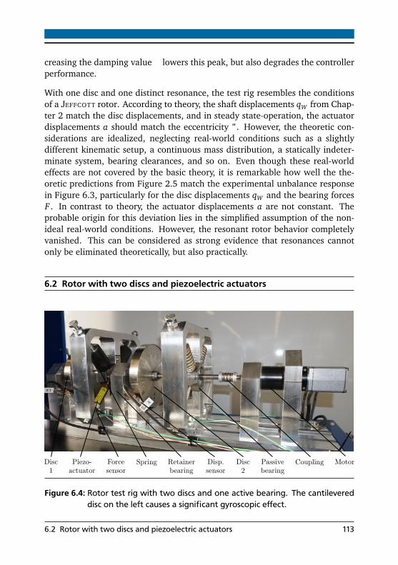
creasing the damping value δ lowers this peak, but also degrades the controllerperformance.

With one disc and one distinct resonance, the test rig resembles the conditionsof a JEFFCOTT rotor. According to theory, the shaft displacements qW from Chap-ter 2 match the disc displacements, and in steady state-operation, the actuatordisplacements a should match the eccentricity ϵ. However, the theoretic con-siderations are idealized, neglecting real-world conditions such as a slightlydifferent kinematic setup, a continuous mass distribution, a statically indeter-minate system, bearing clearances, and so on. Even though these real-worldeffects are not covered by the basic theory, it is remarkable how well the the-oretic predictions from Figure 2.5 match the experimental unbalance responsein Figure 6.3, particularly for the disc displacements qW and the bearing forcesF . In contrast to theory, the actuator displacements a are not constant. Theprobable origin for this deviation lies in the simplified assumption of the non-ideal real-world conditions. However, the resonant rotor behavior completelyvanished. This can be considered as strong evidence that resonances cannotonly be eliminated theoretically, but also practically.

6.2 Rotor with two discs and piezoelectric actuators

Figure 6.4: Rotor test rig with two discs and one active bearing. The cantilevereddisc on the left causes a significant gyroscopic effect.

6.2 Rotor with two discs and piezoelectric actuators 113

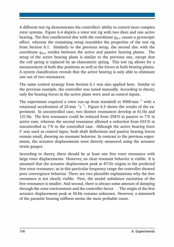
A different test rig demonstrates the controllers’ ability to control more complexrotor systems. Figure 6.4 depicts a rotor test rig with two discs and one activebearing. The first cantilevered disc with the coordinate qW1 causes a gyroscopiceffect; whereas the remaining setup resembles the properties of the test rigfrom Section 6.1. Similarly to the previous setup, the second disc with thecoordinate qW2 resides between the active and passive bearing planes. Thesetup of the active bearing plane is similar to the previous one, except thatthe coil spring is replaced by an elastomeric spring. This test rig allows for ameasurement of both disc positions as well as the forces in both bearing planes.A system classification reveals that the active bearing is only able to eliminateone out of two resonances.

The same control strategy from Section 6.1 was also applied here. Similar tothe previous example, the controller was tuned manually. According to theory,only the bearing forces in the active plane were used as control inputs.

The experiment required a rotor run-up from standstill to 9000 min−1 with arotational acceleration of 25 min−1s−1. Figure 6.5 shows the results of the ex-periment. In uncontrolled case, two distinct resonances develop at 61 Hz and131 Hz. The first resonance could be reduced from 258 N in passive to 7 N inactive case, whereas the second resonance allowed a reduction from 655 N inuncontrolled to 7 N in the controlled case. Although the active bearing forceF was used as control input, both shaft deflections and passive bearing forcesremain small, showing no resonant behavior. In contrast to the previous exper-iment, the actuator displacements were directly measured using the actuatorstrain gauges.

According to theory, there should be at least one free rotor resonance withlarge rotor displacements. However, no clear resonant behavior is visible. It isassumed that the actuator displacement peak at 87 Hz origins in the predictedfree rotor resonance, as in this particular frequency range the controller showedpoor convergence behavior. There are two plausible explanations why the freeresonance is not clearly visible. First, the modal unbalance excitation of thefree resonance is smaller. And second, there is always some amount of dampingthrough the rotor environment and the controller factor δ. The origin of the firstactuator displacement peak at 56 Hz remains unknown. However, a mismatchof the parasitic bearing stiffness seems the most probable cause.

114 6 Experiments

0100200300400500600

Act

.be

arin

gfo

rce

|F|(

N)


0

50

100

150

Psv.

bear

ing

forc

e|F

P|(

N)

00.20.40.60.8

1

Dis

c1

disp

.|q

W1|(

mm

)

00.20.40.60.8

1

Dis

c2

disp

.|q

W2|(

mm

)

25 50 75 100 125 1500

10

20


Act

uato

rdi

sp.

|a|(

µm)

Figure 6.5: Experimental run-up of a rotor test rig with two discs and an activebearing using piezoactuators.

6.2 Rotor with two discs and piezoelectric actuators 115

7 ConclusionThis work deals with the elimination of unbalance-induced forces on generalisotropic rotors with active bearings. Starting with the JEFFCOTT rotor as thesimplest and most representative rotordynamic model, it was reasoned that ac-tive bearings can statically displace the rotor without bearing forces. A newadaptive controller is introduced which uses the bearing forces as input andcontrols the actuator displacements. A subsequent analysis of the controlledsystem reveals that the bearing forces can be completely eliminated for anyrotational speed, also leading to an elimination of the rotor’s resonance. A sta-bility analysis proves that the controller is always stable, a property which canbe attributed to the electronic coupling of the rotor’s perpendicular axes.

The same controller is used to extend the approach to general, isotropic rotors.The analytical closed-loop unbalance response indicates that the controller caneven eliminate the forces of arbitrary rotors, while additionally canceling outtwo critical speeds. Advanced rotordynamic effects such as the influence ofouter and inner damping, gyroscopy and parasitic stiffnesses are thoroughlyinvestigated, solved and discussed.

A physical realization requires a distinction between displacement and forceactuators. The ones aforementioned are inherently stiff and able to supportthe rotor without additional control, while the latter ones require an electronicstabilization. The consistent derivation of control laws for both actuator typesrequires the generalized theory from the previous Chapters. Suitable coordi-nate transformations simplify the controller implementation and allow a directobservation of the rotor’s eccentricity in magnitude and phase. The correctactuator selection is simplified through dimensioning formulas based on theanalytical solutions. Additionally, guidelines how to treat free rotor resonancesare also given.

A universal stability proof for controlled general rotors requires the applicationof LYAPUNOV’s second theorem. The theory’s main advantage is that stability canbe guaranteed for systems of arbitrary dimensions, knowing solely their matrixproperties. However, the problem’s particular matrix inhibited an application ofknown stability theorems. Consequently, a new stability theorem for mechanicalsystems with collocated controller has been derived. Using this theorem, it

117

could be proven that the presented model-free controller is stable for arbitrary,gyroscopic rotors.

The theoretic assumptions are validated in two experiments. The first experi-ment is performed on a test rig with one active piezoelectric bearing plane anda disc attached to a flexible shaft, resembling a JEFFCOTT rotor. The compari-son between passive and active rotor run-up revealed that not only the bearingforces lowered from 95 N to 7 N, but also led to an elimination of the reso-nance, confirming the previous assumptions. The following experiment with amore complex rotor system demonstrated even better force and displacementreductions.

7.1 Scientific contribution

In the introductory Section 1.1 it was indicated that the current problem under-standing is inconsistent and fragmented. This work strives to eliminate theseproblems, giving a clear, consistent problem solution which is compatible withstructural mechanics, control engineering and different active bearing technolo-gies. In particular, the scientific contributions of this work are:

General solution for flexible rotors. This approach gives a general solution forthe unbalance elimination with active bearings on general, flexible rotors. Nat-urally, rigid rotors are also covered by the same theoretical considerations.

Clear principle of operation. The introduced actuator displacements resolve theongoing confusion between filtering and adaptive feedforward compensation.According to Chapter 4, active bearings with force actuators require a controllerthat both supports the rotor and eliminates the unbalance forces, resulting in anotch filter characteristic. For statically stabilized rotors, adaptive feedforwardcompensation can be applied. In this case, the injected harmonic signals areactuator displacements, changing the rotor’s axis of rotation.

No rotor model required. The presented collocated controller removes theunbalance-induced bearing forces even in the absence of a mathematical model.To do so, actuator and sensor must be collocated. Even with a flexible casing,no modeling effort is necessary. Regardless, the controller still requires the ro-tor’s rotational speed.

Elimination of two rotor resonances. This work gave mathematical evidence forwhy two resonances can be eliminated. The root cause can be found in the rankdeficiency of the rotor’s stiffness matrix, reflecting the fact that the rotor can be

118 7 Conclusion

translated and tilted. Moreover, the analytical solution proves that a force freerotor operation at the speed of the free rotor resonance is generally impossible.

Accurate rotordynamics. Many approaches originate from a signal-theoreticviewpoint, often leading to an oversimplification of the underlying rotordynam-ics. The presented approach is compatible with control engineering, structuralmechanics and rotordynamics, resulting in a complete treatment of the problemincluding more complicated rotordynamic effects such as gyroscopy and innerdamping.

Generalized solution. The abstract, technology-independent solution leads toa generalized understanding how active bearings of all types can be used toeliminate unbalance-induced bearing forces. Chapter 4 demonstrated how dif-ferent actuator technologies and arrangements can be linked consistently to thesame system representation, bridging the gap between active magnetic bear-ings, piezoelectric bearings and balancing actuators.

Proven stability. In contrast to all existing approaches, the stability of the con-trolled rotor system was proven analytically. The analysis revealed that thecontrolled system is generally asymptotically stable, except when either the ro-tor’s passive eigenmodes are unobservable or when the rotor is operated atits free resonance frequency. This remarkable solution is based on the discov-ered hyperstable controller and the developed stability proof. Naturally, thisproof is not only limited to the investigated system, but can be applied to anymechanical system with collocated controllers.

7.2 Outlook

The elimination of unbalance-induced bearing forces not only reduces stresses,but also allows for quieter machine operation. The experiments demonstratedan impressive reduction of both forces and displacements, still, there is theoret-ical and practical evidence that both performance and stability are poor in thevicinity of a free rotor resonance. Without external forces, the rotor bends indef-initely – a clearly unwanted behavior. Further analytical approaches could notonly consider the active bearing forces, but also the rotor’s bending energy. Thisleads to the question of how the actuator displacements should be controlled inorder to minimize this energy expression. It is assumed that this problem has ageneral, analytical solution based on specific eigenmodes or other matrix prop-erties. Given these findings, the insight gained will contribute valuable assetsfor the development of new, even more powerful control algorithms.

7.2 Outlook 119

Bibliography[1] ABRAHAM, D. Aktive Beeinflussung von Rotoren: Dissertation, Universität

der Bundeswehr Hamburg. 1992.

[2] ALIZADEH ROSHDI, A. Robuste Regelung zur aktiven Schwingungsdämp-fung elastischer Rotoren mit Piezo-Stapelaktoren: Dissertation, TechnischeUniversität Darmstadt. 2005.

[3] AYRES, F. Schaum’s outline of theory and problems of matrices. Schaum’soutline series. New York: McGraw-Hill, 1962.

[4] BALAS, M. J. “Modal Control of Certain Flexible Dynamic Systems”. In:SIAM Journal on Control and Optimization 16.3 (1978), pp. 450–462.ISSN: 0363-0129. DOI: 10.1137/0316030.

[5] BEARDS, C. F. and WILLIAMS, J. L. “The damping of structural vibrationby rotational slip in joints”. In: Journal of Sound and Vibration 53.3(1977), pp. 333–340. ISSN: 0022460X. DOI: 10.1016/0022-460X(77)90418-7.

[6] BECKER, F., HEINDEL, S., and RINDERKNECHT, S. “Active Vibration Isola-tion of a Flexible Rotor Being Subject to Unbalance Excitation andGyroscopic Effect Using H∞-Optimal Control”. In: Proceedings of the9th IFToMM. Vol. 21. 2015, pp. 1727–1739. DOI: 10.1007/978-3-319-06590-8_142.

[7] BERNSTEIN, D. S. and BHAT, S. P. “Lyapunov Stability, Semistability, andAsymptotic Stability of Matrix Second-Order Systems”. In: Journal ofVibration and Acoustics 117.B (1995), p. 145. ISSN: 07393717. DOI: 10.1115/1.2838656.

[8] BINGULAC, S. “An alternate approach to expanding PA+A’P=-Q”. In:IEEE Transactions on Automatic Control 15.1 (1970), pp. 135–137. ISSN:0018-9286. DOI: 10.1109/TAC.1970.1099386.

[9] BISSELL, C. C. “Stodola, Hurwitz and the genesis of the stability crite-rion”. In: International Journal of Control 50.6 (1989), pp. 2313–2332.ISSN: 0020-7179. DOI: 10.1080/00207178908953500.

121

https://doi.org/10.1137/0316030

https://doi.org/10.1016/0022-460X(77)90418-7

https://doi.org/10.1016/0022-460X(77)90418-7

https://doi.org/10.1007/978-3-319-06590-8_142

https://doi.org/10.1007/978-3-319-06590-8_142

https://doi.org/10.1115/1.2838656

https://doi.org/10.1115/1.2838656

https://doi.org/10.1109/TAC.1970.1099386

https://doi.org/10.1080/00207178908953500

[10] BLEULER, H. et al. “Application of digital signal processors for industrialmagnetic bearings”. In: IEEE Transactions on Control Systems Technology2.4 (1994), pp. 280–289. DOI: 10.1109/87.338647.

[11] BLUTKE, R. et al. “Nichtlineares rotordynamisches Verhalten einesNiederdruckrotors bei nicht zentrierten Quetschöldämpfern”. In: 8. In-ternationale Tagung Schwingungen in rotierenden Maschinen. Vienna,2009.

[12] BORSDORF, M. Aktive Schwingungsminderung elastischer Flugtriebwerk-srotoren mit Piezostapelaktoren unter Berücksichtigung der Dynamikdes Triebwerkgehäuses: Dissertation, Technische Universität Darmstadt.Aachen: Shaker, 2014. ISBN: 3-8440-3007-7.

[13] BROGLIATO, B. Dissipative systems analysis and control: Theory and appli-cations. 2nd ed. London: Springer, 2007. ISBN: 978-1-84628-517-2.

[14] BURROWS, C. R. “An evaluation of some strategies for vibration controlof flexible rotors”. In: International Symposium on Magnetic Suspension.Washington, DC, 1992.

[15] BURROWS, C. R., SAHINKAYA, M., and S. CLEMENTS. “Active Vibration Con-trol of Flexible Rotors: An Experimental and Theoretical Study”. In:Proceedings of the Royal Society of London. Series A, Mathematical andPhysical Sciences 422.1862 (1989), pp. 123–146. ISSN: 00804630.

[16] CAMPOS, R. O. and NICOLETTI, R. “Vibration reduction in vertical wash-ing machine using a rotating dynamic absorber”. In: Journal of theBrazilian Society of Mechanical Sciences and Engineering 37.1 (2015),pp. 339–348. ISSN: 1678-5878. DOI: 10.1007/s40430-014-0151-1.

[17] CHEN, C. and SHIEH, L. “A note on expanding PA + A’P= -Q”. In:IEEE Transactions on Automatic Control 13.1 (1968), pp. 122–123. ISSN:0018-9286. DOI: 10.1109/TAC.1968.1098819.

[18] CHILDS, D. W. Turbomachinery rotordynamics: Phenomena, modeling,and analysis. New York: Wiley, 1993. ISBN: 9780471538400.

[19] DEAUX, R. and EVES, H. Introduction to the Geometry of Complex Num-bers. Newburyport: Dover Publications, 2013. ISBN: 978-0-486-15804-4.

[20] EHRICH, F. F. Handbook of rotordynamics. Malabar: Krieger Pub., 2004.ISBN: 1575242567.

[21] FAIRMAN, F. W. Linear control theory: The state space approach. Chich-ester: Wiley, 1998. ISBN: 0471974897.

122 Bibliography

https://doi.org/10.1109/87.338647

https://doi.org/10.1007/s40430-014-0151-1

https://doi.org/10.1109/TAC.1968.1098819

[22] FERTIG, F. “Untersuchung begrenzender Faktoren für die Anwendungaktiver piezoelektrischer Lager in Rotorsystemen”. MA thesis. TU Darm-stadt, 2016.

[23] FOMI WAMBA, F. Automatische Auswuchtstrategie für einen magnetge-lagerten elastischen Rotor mit Auswuchtaktoren: Dissertation, TechnischeUniversität Darmstadt. 2009.

[24] GASCH, R. “Vibration of large turbo-rotors in fluid-film bearings on anelastic foundation”. In: Journal of Sound and Vibration 47.1 (1976),pp. 53–73. ISSN: 0022460X. DOI: 10.1016/0022-460X(76)90407-7.

[25] GASCH, R. and KNOTHE, K. Strukturdynamik: Band 1: Diskrete Systeme.Berlin: Springer, 1987. ISBN: 3540168494.

[26] GASCH, R., NORDMANN, R., and PFÜTZNER, H. Rotordynamik. Berlin:Springer, 2006. ISBN: 3-540-41240-9.

[27] GENIN, J. and MAYBEE, J. S. “Nonconservative linear systems with con-stant coefficients”. In: Journal of the Institute of Mathematics and itsApplications 8 (1971), pp. 358–370.

[28] GENTA, G. “On a Persistent Misunderstanding of the Role of HystereticDamping in Rotordynamics”. In: Journal of Vibration and Acoustics126.3 (2004), p. 459. ISSN: 07393717. DOI: 10.1115/1.1759694.

[29] GENTA, G. and LING, F. F. Dynamics of Rotating Systems. New York:Springer, 2005. ISBN: 978-0-387-28687-7. DOI: 10 . 1007 / 0 - 387 -28687-X.

[30] GLADWELL, G. and PREUMONT, A. Vibration Control of Active Structures.Vol. 179. Dordrecht: Springer, 2011. ISBN: 978-94-007-2032-9. DOI: 10.1007/978-94-007-2033-6.

[31] GOLUB, G. H. and VAN LOAN, C. Matrix computations. 3rd ed. Johns Hop-kins studies in the mathematical sciences. Baltimore: Johns HopkinsUniversity Press, 1996. ISBN: 0801854148.

[32] GOMIS-BELLMUNT, O. and CAMPANILE, L. F. Design Rules for Actuators inActive Mechanical Systems. London: Springer, 2010. ISBN: 978-1-84882-613-7. DOI: 10.1007/978-1-84882-614-4.

[33] GREINER, W. Classical mechanics: Systems of particles and Hamiltoniandynamics. Heidelberg: Springer, 2010. ISBN: 978-3-642-03434-3.

[34] HAGEDORN, P. and HOCHLENERT, D. Technische Schwingungslehre: Schwin-gungen linearer diskreter mechanischer Systeme. Frankfurt: H. Deutsch,2012. ISBN: 9783817118908.

Bibliography 123

https://doi.org/10.1016/0022-460X(76)90407-7

https://doi.org/10.1115/1.1759694

https://doi.org/10.1007/0-387-28687-X

https://doi.org/10.1007/0-387-28687-X

https://doi.org/10.1007/978-94-007-2033-6

https://doi.org/10.1007/978-94-007-2033-6

https://doi.org/10.1007/978-1-84882-614-4

[35] HAN, F., WU, Q., and GAO, Z. “Initial levitation of an electrostatic bear-ing system without bias”. In: Sensors and Actuators A: Physical 130-131(2006), pp. 513–522. ISSN: 09244247. DOI: 10.1016/j.sna.2005.12.007.

[36] HAN, F. et al. “Nonlinear compensation of active electrostatic bearingssupporting a spherical rotor”. In: Sensors and Actuators A: Physical119.1 (2005), pp. 177–186. ISSN: 09244247. DOI: 10.1016/j.sna.2004.08.030.

[37] HASCH, B. et al. “Model-Based Fault Detection on a Rotor in an Ac-tively Supported Bearing Using Piezoelectric Actuators and the FXLMS-Algorithm”. In: Motion and Vibration Control. Dordrecht: Springer,2009, pp. 123–132. ISBN: 978-1-4020-9437-8. DOI: 10.1007/978-1-4020-9438-5.

[38] HEINDEL, S., BECKER, F., and RINDERKNECHT, S. “Unbalance and reso-nance elimination with active bearings on a Jeffcott Rotor”. In: Me-chanical Systems and Signal Processing 85 (2017), pp. 339–353. DOI:10.1016/j.ymssp.2016.08.016.

[39] HEINDEL, S., MÜLLER, P. C., and RINDERKNECHT, S. “Unbalance and reso-nance elimination with active bearings on general rotors”. In: Journalof Sound and Vibration (2018). ISSN: 0022-460X. DOI: 10.1016/j.jsv.2017.07.048.

[40] HENDERSON, H. and SEARLE, S. “On Deriving the Inverse of a Sum ofMatrices”. In: SIAM Review 23.1 (1981), pp. 53–60. ISSN: 00361445.

[41] HERRMANN, G. Dynamics and stability of mechanical systems with fol-lower forces. Vol. CR-1782. NASA contractor report. Washington, DC:National Aeronautics and Space Administration, 1971.

[42] HERZOG, R. et al. “Unbalance compensation using generalized notchfilters in the multivariable feedback of magnetic bearings”. In: IEEETransactions on Control Systems Technology 4.5 (1996), pp. 580–586.DOI: 10.1109/87.531924.

[43] HEYMAN, J. Structural analysis: A historical approach. Cambridge: Cam-bridge University Press, 1998. ISBN: 0521622492.

[44] HIBBIT, H. D. “Some follower forces and load stiffness”. In: InternationalJournal for Numerical Methods in Engineering 14.6 (1979), pp. 937–941. ISSN: 0029-5981. DOI: 10.1002/nme.1620140613.

124 Bibliography

https://doi.org/10.1016/j.sna.2005.12.007




https://doi.org/10.1007/978-1-4020-9438-5

https://doi.org/10.1007/978-1-4020-9438-5

https://doi.org/10.1016/j.ymssp.2016.08.016

https://doi.org/10.1016/j.jsv.2017.07.048


https://doi.org/10.1109/87.531924

https://doi.org/10.1002/nme.1620140613

[45] HIGUCHI, T., OTSUKA, M., and MIZUNO, T. “Identification of Rotor Unbal-ane and Reduction of Housing Vibration by Periodic Learning Control inMagnetic Bearings”. In: Proceedings of the 3rd International Symposiumon Magnetic Bearings. Alexandria, USA, 1992.

[46] HORST, H. G. Aktive Schwingungsminderung an elastischen Rotoren mit-tels piezokeramischer Aktoren: Dissertation, Technische Universität Darm-stadt. Aachen: Shaker, 2005. ISBN: 3-8322-4150-7.

[47] HURWITZ, A. “Ueber die Bedingungen, unter welchen eine Gleichungnur Wurzeln mit negativen reellen Theilen besitzt”. In: MathematischeAnnalen 46.2 (1895), pp. 273–284. ISSN: 0025-5831. DOI: 10.1007/BF01446812.

[48] HUSEYIN, K., HAGEDORN, P., and TESCHNER, W. “On the stability of lin-ear conservative gyroscopic systems”. In: ZAMP Zeitschrift für ange-wandte Mathematik und Physik 34.6 (1983), pp. 807–815. DOI: 10.1007/BF00949057.

[49] INMAN, D. J. Vibration with Control. Chichester: Wiley, 2006. ISBN:9780470010532. DOI: 10.1002/0470010533.

[50] INSTITUTE OF ELECTRICAL AND ELECTRONICS ENGINEERS (IEEE). Standardon piezoelectricity. New York, N.Y.: Institute of Electrical and ElectronicsEngineers, 1988.

[51] INTERNATIONAL ORGANIZATION FOR STANDARDIZATION (ISO). Mechanical vi-bration: Vibration of rotating machinery equipped with active magneticbearings. First edition. Vol. ISO 14839-4. Geneva, 2012.

[52] JANOCHA, H., BONERTZ, T., and PAPPERT, G. Unkonventionelle Aktoren:Eine Einführung. Zweite ergänzte und aktualisierte Auflage. München:Oldenbourg Verlag, 2013. ISBN: 978-3-486-75692-0.

[53] JEFFCOTT, H. H. “The lateral vibration of loaded shafts in the neighbour-hood of a whirling speed - The effect of want of balance”. In: Philosoph-ical Magazine Series 6 37.219 (1919), pp. 304–314. ISSN: 1941-5982.DOI: 10.1080/14786440308635889.

[54] KAI, Y. L., COPPOLA, V. T., and BERNSTEIN, D. S. “Adaptive autocenter-ing control for an active magnetic bearing supporting a rotor with un-known mass imbalance”. In: IEEE Transactions on Automatic Control 4.5(1996), pp. 587–597. DOI: 10.1109/87.531925.

Bibliography 125

https://doi.org/10.1007/BF01446812

https://doi.org/10.1007/BF01446812

https://doi.org/10.1007/BF00949057

https://doi.org/10.1007/BF00949057

https://doi.org/10.1002/0470010533

https://doi.org/10.1080/14786440308635889

https://doi.org/10.1109/87.531925

[55] KAI, Y. L. et al. “Adaptive virtual autobalancing for a magnetic rotorwith unknown dynamic imbalance”. In: Proceedings of the 34th IEEEConference on Decision and Control. Vol. 3. 1995, pp. 2159–2164. ISBN:0-7803-2685-7. DOI: 10.1109/CDC.1995.480522.

[56] KELVIN, W. T. and TAIT, P. G. Treatise on natural philosophy. Oxford:Clarendon Press, 1867.

[57] KNOSPE, C., TAMIR, S., and FEDIGAN, S. “Design of robust adaptive un-balance response controllers for rotors with magnetic bearings”. In:Proceedings of the 3rd International Symposium on Magnetic SuspensionTechnology. Tallahassee, USA, 1995.

[58] LINDENBORN, O., HASCH, B., and NORDMANN, R. “Vibration Reduction andIsolation of a Rotor in an Actively Supported Bearing Using Piezoelec-tric Actuators and the FXLMS Algorithm”. In: 9th International Confer-ence on Vibrations in Rotating Machinery. 2008.

[59] LÖWIS, J. and RUDOLPH, J. “Adaptive inertial autocentering of a rigid ro-tor with unknown imbalance supported by active magnetic bearings”.In: Proceedings of the 7th International Symposium on Magnetic Bear-ings. Switzerland, 2000.

[60] LUM, K. Y., COPPOLA, V. T., and BERNSTEIN, D. S. “Adaptive Virtual Au-tobalancing for a Rigid Rotor With Unknown Mass Imbalance Sup-ported by Magnetic Bearings”. In: Journal of Vibration and Acoustics120.2 (1998), p. 557. ISSN: 07393717. DOI: 10.1115/1.2893865.

[61] LUNZE, J. Regelungstechnik 1: Systemtheoretische Grundlagen, Analyseund Entwurf einschleifiger Regelungen. 9th ed. Berlin: Springer, 2013.ISBN: 978-3-642-29533-1.

[62] LUNZE, J. Regelungstechnik 2: Mehrgrößensysteme, Digitale Regelung. 7thed. Berlin: Springer, 2013. ISBN: 978-3-642-29561-4.

[63] MAHRENHOLTZ, O. Dynamics of rotors: Stability and system identifica-ton. Vol. no. 273. Courses and lectures. Wien: Springer, 1984. ISBN:9783211818466.

[64] MARKERT, R. Strukturdynamik. Darmstadt: Technische UniversitätDarmstadt, 2011. ISBN: 978-3-9814163-1-2.

[65] MARKERT, R., STRICKA, N., and ZHANG, X. “Unbalance compensation onflexible rotors by magnetic bearings using transfer functions”. In: 8thInternational Symposium on Magnetic Bearings. Mito, Japan, 2002.

126 Bibliography

https://doi.org/10.1109/CDC.1995.480522

https://doi.org/10.1115/1.2893865

[66] MASLEN, E. H. and SCHWEITZER, G. Magnetic Bearings. Berlin: Springer,2009. ISBN: 978-3-642-00496-4. DOI: 10.1007/978-3-642-00497-1.

[67] MEEK, J. L. Matrix structural analysis. New York: McGraw-Hill, 1971.ISBN: 9780070413160.

[68] MESCHEDE, D. and GERTHSEN, C. Gerthsen Physik. Berlin: Springer-Spektrum, 2015. ISBN: 3-662-45976-0.

[69] MINGORI, D. L. “A Stability Theorem for Mechanical Systems With Con-straint Damping”. In: Journal of Applied Mechanics 37.2 (1970), p. 253.ISSN: 00218936. DOI: 10.1115/1.3408497.

[70] MINGORI, D. L. “Stability of whirling shafts with internal and exter-nal damping”. In: International Journal of Non-Linear Mechanics 8.2(1973), pp. 155–160. ISSN: 00207462. DOI: 10.1016/0020-7462(73)90032-2.

[71] MITSCHKE, M. and WALLENTOWITZ, H. Dynamik der Kraftfahrzeuge. 5thed. Wiesbaden: Springer Vieweg, 2014. ISBN: 978-3-658-05068-9.

[72] MÜLLER, P. C. “Allgemeine lineare Theorie für Rotorsysteme ohne odermit kleinen Unsymmetrien”. In: Ingenieur-Archiv 51.1-2 (1981), pp. 61–74. DOI: 10.1007/BF00535955.

[73] MÜLLER, P. C. “Solution of the Matrix Equations AX + X B = −Q andST X+XS = −Q”. In: SIAM Journal on Applied Mathematics 18.3 (1970),pp. 682–687. ISSN: 0036-1399. DOI: 10.1137/0118061.

[74] MÜLLER, P. C. Stabilität und Matrizen: Matrizenverfahren in der Stabil-itätstheorie linearer dynamischer Systeme. Berlin: Springer, 1977. ISBN:0387079815.

[75] MÜLLER, P. C. and SCHIEHLEN, W. O. Forced linear vibrations. Wien:Springer, 1977. ISBN: 978-3-7091-4356-8.

[76] MUSHI, S. E., LIN, Z., and ALLAIRE, P. E. “Design, Construction, andModeling of a Flexible Rotor Active Magnetic Bearing Test Rig”. In:IEEE/ASME Transactions on Mechatronics 17.6 (2012), pp. 1170–1182.ISSN: 1083-4435. DOI: 10.1109/TMECH.2011.2160456.

[77] PALAZZOLO, A. B. et al. “Active Vibration Control of Rotating MachineryWith a Hybrid Piezohydraulic Actuator System”. In: Journal of Engineer-ing for Gas Turbines and Power 117.4 (1995), p. 767. ISSN: 07424795.DOI: 10.1115/1.2815463.

Bibliography 127

https://doi.org/10.1007/978-3-642-00497-1

https://doi.org/10.1115/1.3408497

https://doi.org/10.1016/0020-7462(73)90032-2

https://doi.org/10.1016/0020-7462(73)90032-2

https://doi.org/10.1007/BF00535955

https://doi.org/10.1137/0118061

https://doi.org/10.1109/TMECH.2011.2160456

https://doi.org/10.1115/1.2815463

[78] PALAZZOLO, A. B. et al. “Piezoelectric Pushers for Active Vibration Con-trol of Rotating Machinery”. In: Journal of Vibration Acoustics Stressand Reliability in Design 111.3 (1989), p. 298. ISSN: 07393717. DOI:10.1115/1.3269856.

[79] PALAZZOLO, A. B. et al. “Test and Theory for Piezoelectric Actuator-Active Vibration Control of Rotating Machinery”. In: Journal of Vibra-tion and Acoustics 113.2 (1991), p. 167. ISSN: 07393717. DOI: 10.1115/1.2930165.

[80] PETERS, D. Schwingungsdämpfung elastischer Flugtriebwerksrotoren inQuetschöldämpfern: Dissertation, TU Darmstadt. 2011.

[81] PIAN, T. A study of the structural damping of a simple built-up beam withriveted joints in bending. Cambridge, USA: M.I.T. Aeroelastic and Struc-tures Research Laboratory, 1954.

[82] PINTE, G. et al. “A piezo-based bearing for the active structural acousticcontrol of rotating machinery”. In: Journal of Sound and Vibration 329.9(2010), pp. 1235–1253. ISSN: 0022460X. DOI: 10.1016/j.jsv.2009.10.036.

[83] POPPER, K. Logik der Forschung. Vienna: Springer, 1935. ISBN: 978-3-7091-2021-7. DOI: 10.1007/978-3-7091-4177-9.

[84] PRINGLE, R. “Stability of damped mechanical systems”. In: AIAA Journal3.2 (1965), p. 363. ISSN: 0001-1452. DOI: 10.2514/3.2861.

[85] SCHNEIDER, H. Auswuchttechnik. Berlin: Springer, 2003. ISBN: 3-540-00596-X.

[86] SHAFAI, B. et al. “Magnetic bearing control systems and adaptive forcedbalancing”. In: IEEE Control Systems 14.2 (1994), pp. 4–13. DOI: 10.1109/37.272775.

[87] SHI, J., ZMOOD, R., and QIN, L. “The indirect adaptive feed-forward con-trol in magnetic bearing systems for minimizing the selected vibrationperformance measures”. In: 8th International Symposium on MagneticBearings. Mito, Japan, 2002.

[88] STALLAERT, B., DEVOS, S., and PINTE, G. “Active Structural Acous-tic Source Control of Rotating Machinery Using Piezo Bearings”. In:26th IMAC. Bethel: Society for Experimental Mechanics, 2008. ISBN:9781605600666.

[89] STODOLA, A. Die Dampfturbinen, mit einem Anhang über die Aussichtender Wärmekraftmaschinen und über die Gasturbine. Berlin: Springer,1905.

128 Bibliography

https://doi.org/10.1115/1.3269856

https://doi.org/10.1115/1.2930165

https://doi.org/10.1115/1.2930165



https://doi.org/10.1007/978-3-7091-4177-9

https://doi.org/10.2514/3.2861

https://doi.org/10.1109/37.272775

https://doi.org/10.1109/37.272775

[90] STRIKWERDA, J. C. Finite difference schemes and partial differential equa-tions. 2nd ed. Philadelphia: Society for Industrial and Applied Mathe-matics, 2004. ISBN: 0898715679.

[91] TAMMI, K. Active control of radial rotor vibrations: Identification, feed-back, feedforward, and repetitive control methods. Espoo, Finland: VTTTechnical Research Centre, 2007. ISBN: 9513870073.

[92] THOMSON, W. T. Theory of vibration with applications. Englewood Cliffs,USA: Prentice-Hall, 1972. ISBN: 0139145494.

[93] UNBEHAUEN, H. Regelungstechnik I: Klassische Verfahren zur Analyseund Synthese linearer kontinuierlicher Regelsysteme, Fuzzy-Regelsysteme.Wiesbaden: Vieweg+Teubner, 2008. ISBN: 978-3-8348-9491-5.

[94] VANCE, J. M., MURPHY, B., and ZEIDAN, F. Machinery vibration and rotor-dynamics. Hoboken, USA: Wiley, 2010. ISBN: 978-0-471-46213-2.

[95] VEDENEEV, V. V. “Panel flutter at low supersonic speeds”. In: Journal ofFluids and Structures 29 (2012), pp. 79–96. ISSN: 08899746. DOI: 10.1016/j.jfluidstructs.2011.12.011.

[96] WEIDNER, P. “Zur Stabilität linearer Systeme unter dem Einfluß vonDämpfungs- und Kreiselkräften”. In: ZAMM Zeitschrift für AngewandteMathematik und Mechanik 50.1-4 (1970), pp. 249–250. DOI: 10.1002/zamm.197005001120.

[97] WOODBURY, M. A. Inverting modified matrices: Statistical Research Group,Memo. 42. Princeton University, 1950.

[98] YOO, S. et al. “Optimal Notch filter for active magnetic bearing con-trollers”. In: 2011 IEEE/ASME International Conference on Advanced In-telligent Mechatronics (AIM), pp. 707–711. DOI: 10.1109/AIM.2011.6027087.

[99] ZAJAC, E. E. “Comments on: Stability of Damped Mechanical Systemsand a Further Extension”. In: AIAA Journal 3.9 (1965), pp. 1749–1750.ISSN: 0001-1452. DOI: 10.2514/3.55187.

[100] ZHANG, X. Aktive Regel- und Kompensationsstrategien für magnetgelagerteMehrfreiheitsgrad-Rotoren: Dissertation, Technische Universität Darm-stadt. Herdecke: GCA-Verlag, Jan. 2003. ISBN: 3-89863-118-4.

[101] ZHAO, X. Transmission of Vibration Caused by Unbalance in an AircraftEngine with Active Control Strategies: Dissertation, Technische UniversitätDarmstadt. Aachen: Shaker, 2016. ISBN: 978-3-8440-4271-9.

Bibliography 129

https://doi.org/10.1016/j.jfluidstructs.2011.12.011

https://doi.org/10.1016/j.jfluidstructs.2011.12.011

https://doi.org/10.1002/zamm.197005001120

https://doi.org/10.1002/zamm.197005001120

https://doi.org/10.1109/AIM.2011.6027087

https://doi.org/10.1109/AIM.2011.6027087

https://doi.org/10.2514/3.55187

[102] ZIEGLER, F. Mechanics of Solids and Fluids. New York: Springer, 1995.ISBN: 978-1-4612-6907-6. DOI: 10.1007/978-1-4612-0805-1.

[103] ZIENKIEWICZ, O. C. and CHEUNG, Y. K. The finite element method in struc-tural and continuum mechanics. European civil engineering series. Lon-don: McGraw-Hill, 1967.

[104] ZURMÜHL, R. and FALK, S. Matrizen 1: Grundlagen. 6th ed. Berlin:Springer, 1992. ISBN: 3540539441.

130 Bibliography

https://doi.org/10.1007/978-1-4612-0805-1

Indexacausal system, 25active magnetic bearing, 1, 82,

119actuator

balancing, 66displacement, 57, 59, 65, 68,

71, 75, 79–82force, 5, 65–67, 78–80, 82,

117hydraulic, 67hysteresis, 110linear, 67magnetorestrictive, 67piezoelectric, 1, 3, 36, 67,

109shape memory alloy, 67thermal expanison, 67

bandwidth, 67, 71, 73bearing invariance, 60, 85BETTI, 30BODE plot, 23

circulatoryforces, 51, 101matrix, 53, 91, 101, 108

collocation, 17, 99, 102, 103,110

complexconjugate transpose, 99coordinates, 7, 9, 25, 26,

54–56, 68, 70, 98eigenvectors, 56

computer algebra system, 95–97,99

conservative, 14, 56, 98controller

adaptive, 66, 68, 117Integral Force Feedback, 86

convergence, 14, 114counterrotating, 16, 22critical speed, 1–3, 10, 20, 47, 85,

117cut-off frequency, 71

dampingcomplete, 91, 93inner, 50–53, 73, 101, 117,

119outer, 50, 52, 117pervasive, 93

decompositionbimodal, 56modal, 35, 41, 56

definitepositive, 34, 91, 95, 100, 101,

104, 108positive semi-, 91–95, 100,

101, 103, 104, 108dynamic bearing stiffness, 81dynamic stiffness matrix, 52

encoder, 68, 70EULER’s identity, 70

FÖPPL, 1, 7

131

failsafe, 75finite elemente software, 32follower forces, 101footpoint excitation, 12, 38forward difference, 70, 82frequency response function, 23

generalized coordinates, 55gyroscopic

effect, 47, 53–55, 75, 114matrix, 54, 55, 91, 98, 101moments, 14, 56stiffening, 56

HAMILTON, 90-ian, 90, 91, 94–97, 100,

102health monitoring, 5, 20, 70hermitian, 99, 100, 102

form, 100, 103skew-, 51, 55, 99

higher harmonics, 73, 111homogeneous solution, 10, 14, 16,

60, 74, 90HOOKE, 31HURWITZ, 21, 87, 89

-determinants, 21, 23, 88,89

hyperstability, 22, 23, 25, 119

identity matrix, 18imaginary unit, 14, 26, 54inherent stiffness, 65, 66, 78,

117INMAN, 88instability, 2, 4, 21, 50, 53, 78,

104, 111, 112aeroelastic, 101static, 11

invertible matrix, 18, 40, 103

ISO 1940, 84isotropic rotor, 5, 7, 29, 87, 117

JEFFCOTT, 1, 7, 10-rotor, 5, 7, 11, 18, 36, 38, 41,

45, 46, 70, 78, 80, 83,84, 87, 104, 113, 117,118

jet engine, 75

KIMBALL, 50KRONECKER-product, 94

LARSONNEUR, 2, 3DE LAVAL, 1, 10LEVERRIER-FADDEEV-matrices, 94LYAPUNOV, 88, 91, 93, 94, 100

-equation, 94, 96–100-function, 101-stability, 5, 87, 88, 91, 92,

95, 99, 105second theorem, 90, 117

MÜLLER, 87, 100mass coordinates, 8, 34, 50Mathematica, 95Matlab, 95matrix inversion lemma, 41MAXWELL, 30MINGORI, 101, 102

natural vibration, 10negative frequency, 25NEWKIRK, 50NEWTON, 8, 13, 34noncommutative matrix algebra,

97nonconservative, 101noninvertible matrix, 93

O-ring, 75

132 Index

observability, 57, 92, 101, 102,105

HAUTUS, 92, 105KALMAN, 92

PALAZZOLO, 1parallel path, 52, 57, 59, 75, 76parasitic resonances, 58particular solution, 10, 14, 18,

74passivity, 22perpendicularity, 14, 54phase shift, 24polar moment of inertia, 53–55POPOV, 22principal axis of inertia, 2, 3, 70

quadratic form, 90, 91, 98

RALEIGH dissipation function, 90,91, 94

rank deficiency, 32, 42, 44, 47, 56,58, 118

reaction force, 11, 30, 36, 52, 57,78, 79

reference input, 12regular matrix, 32, 34, 100, 103resolver, 68retainer bearings, 84rigid body modes, 3, 31, 42runout, 2

SCHUR complement, 100, 103,104

shaft coordinates, 8, 34, 43Simulink Real-Time, 110

Squeeze-Film-Damper, 75stability

asymptotic, 22, 89, 91–93,101, 102, 105, 108,119

conditional, 16, 22, 26marginal, 92, 101, 105

staticcondensation, 32, 55determinacy, 11, 34, 36, 79,

104indeterminacy, 38, 110, 113

STODOLA, 53, 87strain gauge, 110support excitation, 12symmetric matrix, 30, 35, 51, 91,

94, 98skew-, 26, 98, 101

technology independence, 4, 65,119

THOMSON-TAIT, 87transversal moment of inertia,

53–55

unit displacements, 30

virtual position setpoint, 79, 80virtual sensor, 76virtual work, 30, 51

whirlbackward, 25, 56forward, 25, 56

WOODBURY matrix identity, 41,103

Index 133

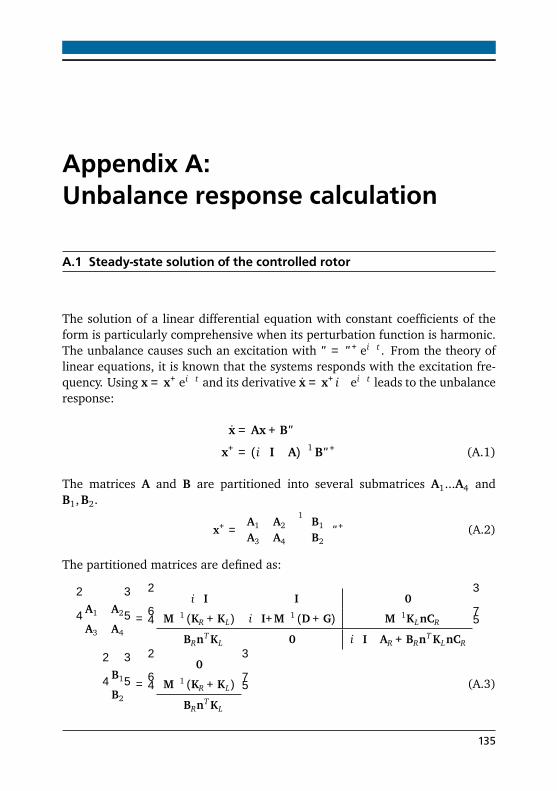
Appendix A:Unbalance response calculation

A.1 Steady-state solution of the controlled rotor

The solution of a linear differential equation with constant coefficients of theform is particularly comprehensive when its perturbation function is harmonic.The unbalance causes such an excitation with ϵ = ϵ+ eiΩt . From the theory oflinear equations, it is known that the systems responds with the excitation fre-quency. Using x = x+ eiΩt and its derivative x = x+iΩeiΩt leads to the unbalanceresponse:

x = Ax+Bϵ

x+ = (iΩI−A)−1 Bϵ+ (A.1)

The matrices A and B are partitioned into several submatrices A1...A4 andB1,B2.

x+ =

A1 A2

A3 A4

−1 B1

B2

ϵ+ (A.2)

The partitioned matrices are defined as:

⎡

⎣

A1 A2

A3 A4

⎤

⎦=

⎡

⎢

⎣

iΩI −I 0

M−1 (KR +KL) iΩI+M−1 (D+G) −M−1KLnCR

−BRnT KL 0 iΩI−AR +BRnT KLnCR

⎤

⎥

⎦

⎡

⎣

B1

B2

⎤

⎦=

⎡

⎢

⎣

0

M−1 (KR +KL)

−BRnT KL

⎤

⎥

⎦(A.3)

135

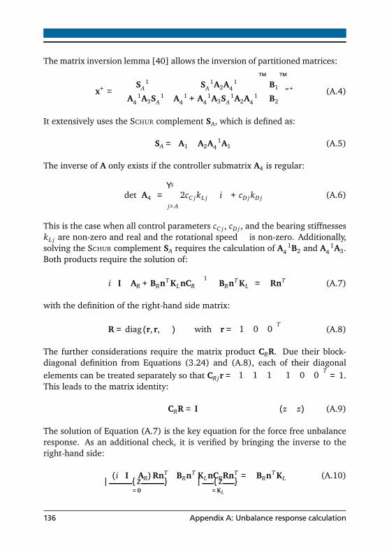
The matrix inversion lemma [40] allows the inversion of partitioned matrices:

x+ =

S−1A −S−1

A A2A−14

−A−14 A3S−1

A A−14 +A−1

4 A3S−1A A2A−1

4

B1

B2

ϵ+ (A.4)

It extensively uses the SCHUR complement SA, which is defined as:

SA =

A1 −A2A−14 A1

(A.5)

The inverse of A only exists if the controller submatrix A4 is regular:

det

A4

=z∏

j=A

2cC jkL jΩ

iΩ+ cD jkD j

(A.6)

This is the case when all control parameters cC j , cD j , and the bearing stiffnesseskL j are non-zero and real and the rotational speed Ω is non-zero. Additionally,solving the SCHUR complement SA requires the calculation of A−1

4 B2 and A−14 A3.

Both products require the solution of:

iΩI−AR +BRnT KLnCR

−1 −BRnT KL

= −RnT (A.7)

with the definition of the right-hand side matrix:

R = diag (r, r, · · · ) with r =

1 0 0T

(A.8)

The further considerations require the matrix product CRR. Due their block-diagonal definition from Equations (3.24) and (A.8), each of their diagonalelements can be treated separately so that CRjr =

1 1 1

·

1 0 0T

= 1.This leads to the matrix identity:

CRR = I (z × z) (A.9)

The solution of Equation (A.7) is the key equation for the force free unbalanceresponse. As an additional check, it is verified by bringing the inverse to theright-hand side:

− (iΩI−AR)RnT

=0

−BRnT KLnCRRnT

=KL

= −BRnT KL (A.10)

136 Appendix A: Unbalance response calculation

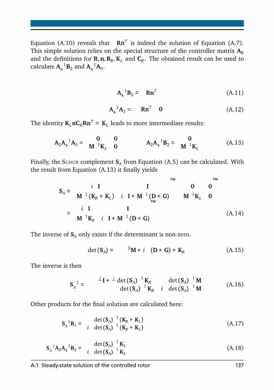
Equation (A.10) reveals that −RnT is indeed the solution of Equation (A.7).This simple solution relies on the special structure of the controller matrix ARand the definitions for R,n,BR,KL and CR. The obtained result can be used tocalculate A−1

4 B2 and A−14 A3.

A−14 B2 = −RnT (A.11)

A−14 A3 =

−RnT 0

(A.12)

The identity KLnCRRnT = KL leads to more intermediate results:

A2A−14 A3 =

0 0M−1KL 0

A2A−14 B2 =

0M−1KL

(A.13)

Finally, the SCHUR complement SA from Equation (A.5) can be calculated. Withthe result from Equation (A.13) it finally yields

SA =

iΩI −I

M−1 (KR +KL) iΩI+M−1 (D+G)

−

0 0

M−1KL 0

=

iΩI −I

M−1KR iΩI+M−1 (D+G)

(A.14)

The inverse of SA only exists if the determinant is non-zero.

det (SA) =

−Ω2M+ iΩ (D+G) +KR

(A.15)

The inverse is then

S−1A =

− iΩ I+ i

Ω det (SA)−1 KR det (SA)

−1 M− det (SA)

−1 KR iΩdet (SA)−1 M

(A.16)

Other products for the final solution are calculated here:

S−1A B1 =

det (SA)−1 (KR +KL)

iΩdet (SA)−1 (KR +KL)

(A.17)

S−1A A2A−1

4 B2 =

det (SA)−1 KL

iΩdet (SA)−1 KL

(A.18)

A.1 Steady-state solution of the controlled rotor 137

A−14 A3S−1

A A2A−14 B2 = −RnT det (SA)

−1 KL (A.19)

A−14 A3S−1

A =

−RnT

iΩ det (SA)

−1 KR −iΩ I

−RnT

det (SA)−1 M

(A.20)

A−14 A3S−1

A B1 = −RnT det (SA)−1 (KR +KL) (A.21)

The final unbalance response can be calculated using Equation (A.4).

x+ =

S−1A B1 − S−1

A A2A−14 B2

−A−14 A3S−1

A B1 +A−14 B2 +A−1

4 A3S−1A A2A−1

4 B2

ϵ+ (A.22)

and finally

x+ =

⎡

⎢

⎣


−1KR

iΩ


−1KR

RnT


−1KR −RnT

⎤

⎥

⎦ϵ+ (A.23)

A.2 Unbalance response with rotating damping

In this section, the unbalance response with rotating damping is calculated.Therefore, two damping matrices are introduced: the one with nonrotatingdamping D and the one with rotating damping DI . The special feature of lattermatrix is that it appears as a summand with the stiffness matrices KR and KL .Although the damping matrix DI is symmetric, the coordinate transformationto inertial coordinates made it skew-symmetric. The solution of the state-spacesystem

x = Ax+Bϵ

with the matrices

A =

⎡

⎢

⎣

0 I 0

−M−1 (KR +KL − iΩDI ) −M−1 (D+DI +G) M−1KLnCR


⎤

⎥

⎦


B =

⎡

⎢

⎣

0

M−1 (KR +KL)

−BRnT KL

⎤

⎥

⎦(A.24)

can be calculated in the same fashion as it was done in Appendix A.1. Forbrevity, only the differences in the calulation are reported here. Most notably,the SCHUR complement of Equation (A.14) has changed:

SA =

⎡

⎣

iΩI −I

M−1 (KR − iΩDI ) iΩI+M−1 (D+DI +G)

⎤

⎦ (A.25)

A short calculation reveals that the determinant of SA does not contain the ro-tating damping matrix DI :

det (SA) =


(A.26)

The matrix inverse S−1A then yields:

S−1A =

⎡

⎣

− iΩ I+ i

Ω det (SA)−1 (KR − iΩDI ) det (SA)

−1 M

− det (SA)−1 (KR − iΩDI ) iΩdet (SA)

−1 M

⎤

⎦ (A.27)

Despite the fact that the matrix inverse has changed compared to Equa-tion (A.16), the Equations (A.17)-(A.21) show that the only products formedwith the SCHUR complements are S−1

A A2 and S−1A B1. It turns out that the prod-

ucts are left unchanged, because both A2 and B1 contain null matrices. Theunbalance response for the system with inner and outer damping is then:

x+ =

⎡

⎢

⎣


−1KR

iΩ


−1KR

RnT


−1KR −RnT

⎤

⎥

⎦ϵ+ (A.28)

As a conclusion, the rotating damping DI has no influence on the steady-statesolution.

A.2 Unbalance response with rotating damping 139

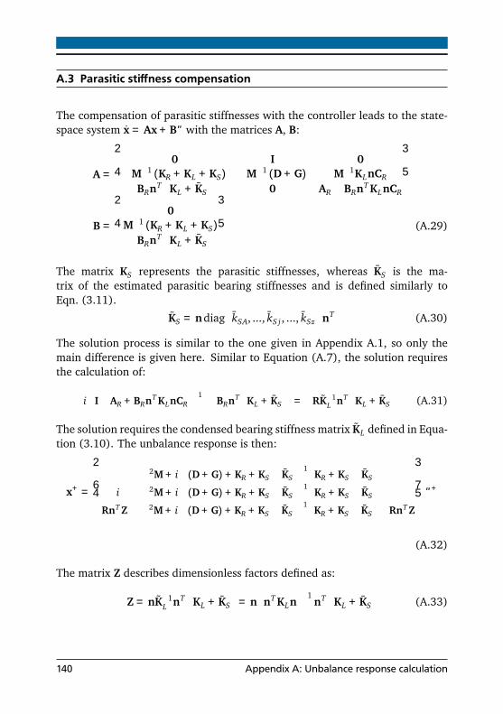
A.3 Parasitic stiffness compensation

The compensation of parasitic stiffnesses with the controller leads to the state-space system x = Ax+Bϵ with the matrices A, B:

A =

⎡

⎣

0 I 0−M−1 (KR +KL +KS) −M−1 (D+G) M−1KLnCR

BRnT

KL + KS

0 AR −BRnT KLnCR

⎤

⎦

B =

⎡

⎣

0M−1 (KR +KL +KS)−BRnT

KL + KS

⎤

⎦ (A.29)

The matrix KS represents the parasitic stiffnesses, whereas KS is the ma-trix of the estimated parasitic bearing stiffnesses and is defined similarly toEqn. (3.11).

KS = ndiag

kSA, ..., kS j , ..., kSz

nT (A.30)

The solution process is similar to the one given in Appendix A.1, so only themain difference is given here. Similar to Equation (A.7), the solution requiresthe calculation of:

iΩI−AR +BRnT KLnCR

−1 −BRnT

KL + KS

= −RK−1L nT

KL + KS

(A.31)

The solution requires the condensed bearing stiffness matrix KL defined in Equa-tion (3.10). The unbalance response is then:

x+ =

⎡

⎢

⎣

−Ω2M+ iΩ (D+G) +KR +KS − KS

−1 KR +KS − KS

iΩ


−1 KR +KS − KS

RnT Z


−1 KR +KS − KS

−RnT Z

⎤

⎥

⎦ϵ+

(A.32)

The matrix Z describes dimensionless factors defined as:

Z = nK−1L nT

KL + KS

= n

nT KLn−1

nT

KL + KS

(A.33)


A.4 Unbalance response with casing

The approach starts with the equations of motion for rotor and casing. To dif-ferentiate between both, additional subindices are introduced. The subindex r(rotor) is appended to all vectors and matrices of the rotating parts, while thesupport structure is augmented with the subindex c (casing).

Rotor: Mr qSr + (Dr +Gr) qSr +KRrqW r = −Fr

Casing: Mc qSc + (Dc +Gc) qSc +KRcqSc = −Fc (A.34)

The matrices Mc ,Dc ,Gc ,KRc are arbitrary mass, damping, gyroscopic and stiff-ness matrices of the casing. Furthermore, the unbalance acts only on the rotat-ing part with the eccentricity ϵr , whereas the eccentricity ϵc = 0 for the casing.The force on the individual active bearings are then:

F = KL (qW r − qSc − a) (A.35)

In accordance with the previous definitions, the vector F contains the bearingforces FA, ..., Fz and a represents the condensed actuator forces. The condensedbearing stiffness matrix KL was defined in Equation (3.10), the condensed vec-tors qW c , qSc that only contain the j coordinates for the attached bearings. Thetransformation matrix nr uses the definition from Equation (3.8) and convertsthe rotor’s nodes qW r to their condensed counterparts qW r .

qW r = nTr qW r , qSc = nT

c qSc (A.36)

The same principle applies for the transformation of bearing forces, but withthe peculiarity that the forces which act on the rotor are opposing the ones ofthe fixed part:

Fr = nr F, Fc = −nc F (A.37)

With the kinematic relations from Equation (3.6) , the active bearing forces thatact on both systems can be expressed as:

A.4 Unbalance response with casing 141

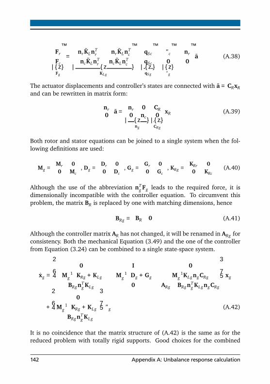
Fr

Fc

Fg

=

nr KLnTr −nr KLnT

c

−ncKLnTr ncKLnT

c

KLg

qSc

qSc

qSg

−

ϵc

0

ϵg

−

nr

0

a

(A.38)

The actuator displacements and controller’s states are connected with a = CRxRand can be rewritten in matrix form:

nr0

a =

nr 00 nc

ng

CR0

CRg

xR (A.39)

Both rotor and stator equations can be joined to a single system when the fol-lowing definitions are used:

Mg =

Mr 00 Mc

, Dg =

Dr 00 Dc

, Gg =

Gr 00 Gc

, KRg =

KRr 00 KRc

(A.40)

Although the use of the abbreviation nTg Fg leads to the required force, it is

dimensionally incompatible with the controller equation. To circumvent thisproblem, the matrix BR is replaced by one with matching dimensions, hence

BRg =

BR 0

(A.41)

Although the controller matrix AR has not changed, it will be renamed in ARg forconsistency. Both the mechanical Equation (3.49) and the one of the controllerfrom Equation (3.24) can be combined to a single state-space system.

xg =

⎡

⎢

⎣

0 I 0

−M−1g

KRg +KLg

−M−1g

Dg +Gg

M−1g KLgngCRg

BRgnTg KLg 0 ARg −BRgnT

g KLgngCRg

⎤

⎥

⎦xg

+

⎡

⎢

⎣

0

M−1g

KRg +KLg

−BRgnTg KLg

⎤

⎥

⎦ϵg (A.42)

It is no coincidence that the matrix structure of (A.42) is the same as for thereduced problem with totally rigid supports. Good choices for the combined


matrices allow the exploitation of the already derived solution, generalizing itfurther. However, the unbalance response calculation from A.1 relies on simpli-fications and identities for some matrix operations. Before accepting the finalsolution, it has to be checked if each simplification also holds for this systemwith modified matrices. A central role takes the SCHUR complement SA, whichwas calculated in Equations (A.5)-(A.10). A dimensional analysis reveals thatthe matrix R from Equation (A.8) cannot be part of the solution. A new matrixRg is defined as:

RG =

R R

(A.43)

A central role in the verification of Equation (A.10) is the matrix identity KL =KLnCRRnT . However, it is still unclear if the matrix identity is also satisfiedfor:

KLg = KLgngCRgRgnTg (A.44)

Despite being immediately obvious, the choice of Rg indeed satisfies this matrixidentity. With this result, it is easy to show that Equations (A.7) and (A.10) alsohold. Since there are no further obstacles to overcome, the unbalance responseof Appendix A.1 not only solves the problem of the rotor with fixed supports,but is also valid for the general case.

qSg =

−Ω2Mg + iΩ

Dg +Gg

+KRg

−1KRgϵ

+g eiΩt (A.45)

A.4 Unbalance response with casing 143

Documents

tuprints.ulb.tu-darmstadt.de · Unbalance and Resonance Elimination on General Rotors with Active Bearings Am Fachbereich Maschinenbau an der Technischen Universität Darmstadt zur