1. INTRODUCTION

In previous works, Sampaio de Sousa e Ramos de Sousa (1999a, 1999b) used non-parametric techniques - DEA (Data Envelopment Analysis) and FDH (Free Disposal Hull) to measure the level of technical efficiency for the Brazilian municipalities. This research permitted to evaluate the performance of the Brazilian cities and furnished an instrumental flexible enough to be used for evaluating local governments. Yet, we should emphasize the exploratory nature of those works. Besides the data set limitations, the computed indicators should be careful used, as the inefficiencies found are not explained only by managerial incompetence or by the inexistence of satisfactory incentive schemes to assure an adequate functioning of the communes. Due to the deterministic nature of non-parametric models, such inefficiencies may also reflect the presence of atypical observations, measurement errors, omitted variables and other statistical discrepancies. Additionally, in DEA methods, heterogeneity of the data set may aggravate this problem and underestimate, substantially, efficiency scores as in those methods, the frontier is constituted by a small number of municipalities. This problem becomes particularly preoccupant when the data set is both huge and diverse, as is the case of the Brazilian municipalities. Here, the size and heterogeneity of sample makes it virtually impossible to manually detect the outliers and/or errors, thus requiring the use of some automatic approach. Therefore, to make efficiency scores credible it is necessary to use an adequate procedure to correct those indices for outliers. Only then, one may hope to obtain truly representative estimators, which could be useful for the decision making process. Moreover, those inefficiencies may also be caused by the existence of exogenous factors, that are out of the control of the municipalities such as natural and climatic characteristics, political factors, demographic and socio economic features, which have not been taken into consideration on the previous non-parametric analysis. The importance of those aspects has been pointed out by several studies, using different techniques, in an attempt to separate the influence of those factors from the ones associated with productive efficiency and thus get a “pure” measure of technical efficiency (see Lovell, Walters and Wood (1990), Kalirajan (1990), McCarty e Yaisawarng (1993), Gillen e Lall (1997) e Yu (1998)). Hence, the key issue here is to identify the conditioning factors lying behind the efficiency scores. In this paper we estimate efficiency indices for the Brazilian municipalities by using Bootstrap and Jackknife resampling techniques to eliminate the effect of outliers and possible errors in the data set, using both the constant and variable returns to scale variants of the DEA method. After computing the efficiency scores we use techniques of spatial econometrics and quantile regressions to investigate the determinants of those computed efficiency scores. This paper is organized as follows. Section 2 presents the methodology used to compute the outliers-corrected DEA efficiency scores. Section 3 briefly comments the data set and the choice of the indicators used as proxies for the supply of local public services. Section 4 discusses the non-parametric efficiency estimators obtained. Section 5 presents the econometric results of the analysis of the conditional factors underlying those scores. Finally, Section 6 summarizes the main conclusions of our study.

2. DATA ENVELOPMENT ANALYSIS MEASUREMENTS OF TECHNICAL EFFICIENCY Non-parametric deterministic approaches to efficiency measurements are characterized by the use of very weak assumptions concerning the reference technology. Except for the usual regularity axioms such as the bounded-ness and closed-ness of the technology, those methods rely on very simple hypothesis such as convexity and strong free disposability in inputs and outputs. In particular, the linear programming based techniques, known as DEA (Data Envelopment Analysis).1 Below we will briefly describe those methodologies.

2. 1 Data Envelopment Analysis Reference Technology For each decision making unit (DMU), the technology transforms nonnegative inputs xk = ( xk1, ..., xkN ) ∈ ℜ+

N into the nonnegative outputs yk = ( yk1,..., ykM) ∈ ℜ+M. For the

input-based measures of technical efficiency, the technology is represented by its production possibility set T = (x,y): x can produce y, the set of all feasible input-output vectors. The input correspondence for the DEA reference technology, characterized by constant returns to scale (C) and strong disposability of inputs (S) defines a piecewise linear technology constructed on the basis of observed input-output combinations:

(2.1) L(y |C, S) = x: y ≤ zM, zN ≤ x, z ∈ ℜ+

K , y ∈ ℜ+M

The k x m matrix M contains the m observed outputs of each of the k observations in the data set, N is the k x n matrix of observed inputs and z is the 1 x k vector of intensity parameters.2 Now, for each activity, the technical efficiency on inputs, Fi, may be defined, as: (2.2) Fi (yk, xk | C,S) = minθ: θ x ∈ L(yk | C,S) This radial efficiency measure is always situated between zero and one. The efficient production on the isoquant is indicated by the unity. Thus, 1-θ represents the proportion at which the inputs could be reduced without changing the production. By using the technology specified in (2.1), technical efficiency for the municipality k may be computed as the solution for the following linear program: (2.3) Fi (yk, xk | C,S) = θ DEA-CCR = min θ θ , z subject to: θ xnk - Σk=1

K zk xnk

≥ 0 n = 1,..., N

Σj=1K zk

ykm ≥ yrk, m = 1,..., M

θ

, zk ≥ 0 k = 1,..., K

2

This first version of the DEA methodology – henceforth mentioned as CCR – implies strong restrictions concerning the production set. In particular, this methodology presupposes constant returns to scale. This hypothesis can be easily relaxed by modifying the restrictions on the intensity vector, z. Maintaining the hypothesis of strong disposability, Färe, Grosskopf and Lovell (1985, 1994) extended this technique to include the existence of non increasing returns to scale by adding, to program (2.3), the following restriction: (2.4) ∑K

k=1 zk ≤ 1 Here, the sum of the intensity variables cannot exceed the unity implying that the different activities can be contracted but cannot be expanded limitlessly. In the case of variable returns to scale model (Banker, Charnes and Cooper (1984)), activities cannot be expanded or contracted radially without limits and radial contractions to the origin are also excluded. The feasible set of activities is formed by all convex combination of observed activities, located on the boundary of the productive set. We have, thus, increasing returns for low levels of production and decreasing returns for higher levels. It is well known that the efficiency indexes associated with this technology - henceforth denominated DEA-BCC – are obtained by imposing equality on restriction (2.4). 2.2 The Leverage and “Jackstrap” Procedure As previously mentioned, one of the main drawbacks of DEA is that the efficiency scores are rather sensitive to presence of DMUs that perform extremely well (so called outliers), which may stem from some outstanding practice, or may simply be the result of errors in the data. In either case, the results for the remaining DMUs become shifted towards lower efficiency values, the efficiency frequency distribution becomes highly asymmetric, and the overall efficiency scale becomes non-linear. Several approaches have been proposed to deal with this effect (Wilson (1993,1995), Banker and Gifford (1985), Seaver and Triantis (1989)) but they largely depend on manual inspection of data, which becomes virtually impossible for large data sets, like the one used in this paper. To tackle this issue, we will use a recently proposed method by Stosic and Sampaio de Sousa (2003), based on a combination of Bootstrap and Jackknife resampling schemes, for automatic detection of outliers. This approach is based on the concept of leverage, that is, the effect produced on the outcome of DEA efficiencies of all the other DMUs, when the observed DMU is removed from the data set (See Cribari-Neto and Zarkos (2002). The leverage information is calculated for each DMU, and it is then used to detect outliers and errors in the data set, and automatically eliminate them, or just reduce their influence. The underlying idea is that outliers are expected to show leverage much above the mean and then should be selected with lower probability than the other DMUs. Below we will briefly describe this procedure. Leverage of a single observed DMU might be understood as the quantity that measures the impact of removal of the DMU from the data set, on the efficiency scores of all the other DMUs. Formally, it may be defined as the standard deviation of the efficiency measures before and after the removal. The most straightforward possibility is to perform Jackknife resampling technique as follows. One first applies DEA for each of the DMUs using the unaltered original data set, to obtain the set of efficiencies Kkk ,,1| …= θ . Then, one by one DMU is successively removed, and each time the

3

set of efficiencies jkKkkj ≠= ;,,1|* …θ

( )

is recalculated, where index represents the removed DMU. The leverage of j-th DMU may then be defined as standard deviation

Kj ,,1…=

.1

;1

2*

−

−∑≠=

K

K

jkkkkj θθ

~

K,,1…

kb~

K/

≥

<

K

K

k

k

log~~,0

log~~,1

(2.5) =j

While rather straightforward, this direct approach is extremely computationally intensive, and may turn unfeasible for very large data sets with the available computer resources. More precisely, removing each of the K DMUs from the data set and then performing (K-1) DEA calculations requires solving K(K-1) linear programs, and may become prohibitively computationally expensive for large K. We therefore proposed a more efficient stochastic procedure, which combines Bootstrap resampling with the above Jackknife scheme as follows: 1. Select randomly a subset of L DMUs (typically 10% of K) and perform the above

procedure to obtain subset leverages 1k , where index takes on L (randomly selected) values from the set .

k

2. Repeat the above step B times, accumulating the subset leverage information for all randomly selected DMUs (for B large enough, each DMU should be selected roughly times). BLnk ≈

3. Calculate mean leverage for each DMU as

k

n

bkb

k n

k

∑== 1

~~

and the global mean leverage as

K

K

kk∑

== 1

~~

This completes the first phase of the proposed approach. In the second phase, one can either use the leverage information to detect and simply eliminate outliers from the data set, or one can implement Bootstrap method to produce confidence intervals and bias information, using leverage information to reduce the probability of selecting the outliers in the stochastic resampling process. In this paper we used the Heaviside step function, given by

(2.6) ( )

=P k~

4

Here the threshold level Klog~ was chosen in order to take into account the sample size, so that for e.g. K=1000 a DMU with leverage greater than three times the global mean is rejected. 3. DATA The implementation of the above outlined methodologies requires information about aggregate total costs and other relevant inputs, as well as the amount of public services available to the population for the municipalities (outputs). Initially, information for the 5264 Brazilians municipalities was collected. We excluded data for municipalities for which some key information was missing. These way 620 communes were dropped since 493 of them had a recorded population of zero and 127 others had no data on current expenditure.3 The final data set was composed of 4796 municipalities. All data refers to the year 2000. 3.1 Input and Output Indicators for the Brazilian Municipalities A list of inputs and outputs are provided in Table 3.1, together with their respective sources, and the public service they are supposed to represent.

Table 3.1 - Input and Output Indicators and the Corresponding Municipal Services – 2000 Input and Output Indicators Source Municipal Services of which

indicators serve as proxies

- Input Indicators 1. Current spending STN1 Aggregate total costs 2. Number of teachers Censo Escolar/MEC Personnel input 3. Rate of infant mortality IBGE2 Public health services 4. Hospital and health services IBGE Public health services - Output Indicators 1.Total resident population IBGE Administrative services 2. Literate population MEC3 Educational services 3. Enrollment4 per school Censo Escolar/MEC Educational services 4. Student attendance per school Censo Escolar/MEC Educational services 5. Students approved per school Censo Escolar/MEC Educational services 6. Students in the right class per school Censo Escolar/MEC Educational services 7. Domiciles with access to safe water IBGE Health and housing conditions 8. Domiciles with access to sewage system IBGE Health and housing conditions 9. Domiciles with access to garbage collection

IBGE Health and housing conditions

Sources: 1: STN - Secretaria do Tesouro Nacional (National Treasure Secretariat); 2: IBGE - Instituto Brasileiro de Estatística, Censo Demográfico de 2000; 3: MEC - Ministério da Educação; 4: All data refer to primary and secondary municipal schools.

Aggregate total costs were computed as the value of municipal current spending. The other inputs used were the number of teachers (as a proxy for personnel inputs), the number of hospital and health centers, as they are the main providers of health services. The rate of infant mortality stands as an input because if health services are efficient, this indicator should be as low as possible. As for output measures, due to the impossibility of quantifying directly the supply of public services, they were approximated by a set of selected indicators, which are observable factors taken as

5

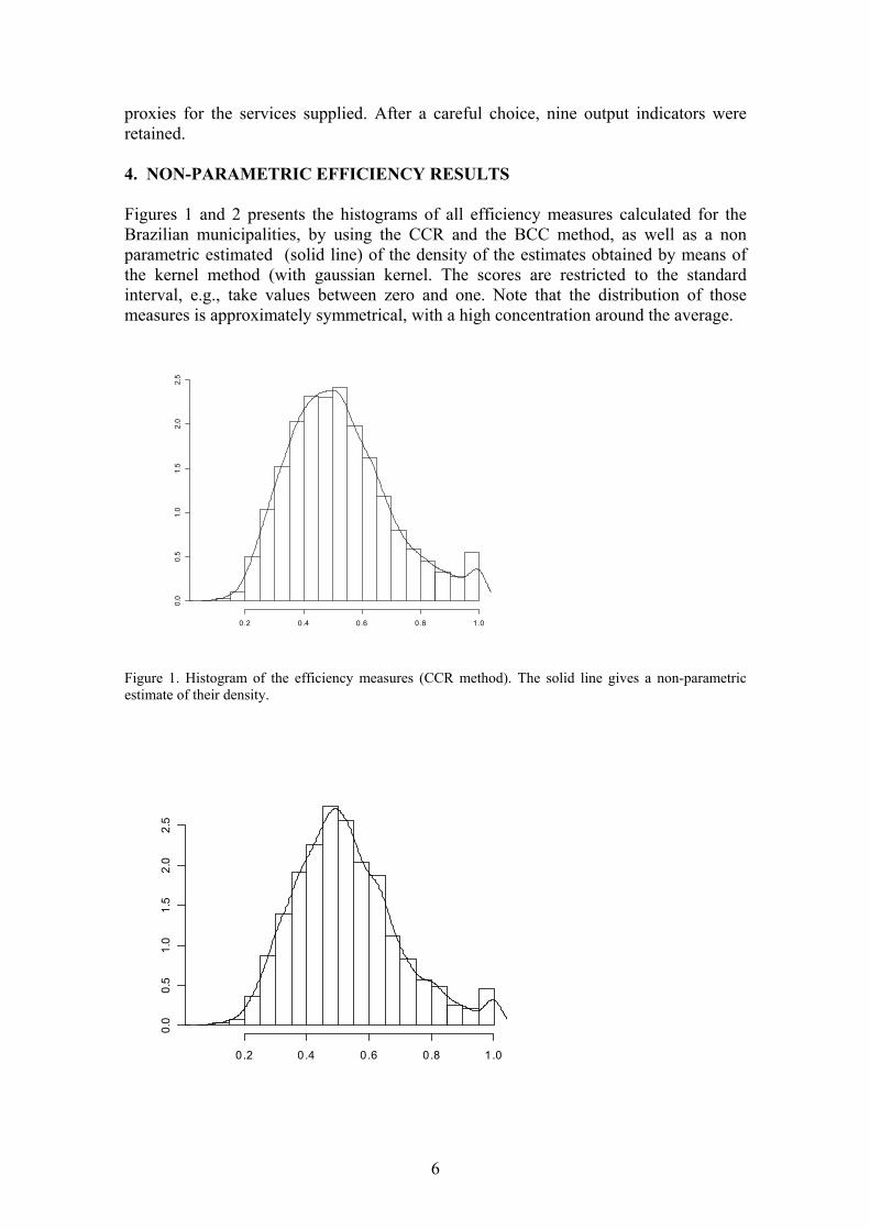
proxies for the services supplied. After a careful choice, nine output indicators were retained. 4. NON-PARAMETRIC EFFICIENCY RESULTS

Figures 1 and 2 presents the histograms of all efficiency measures calculated for the Brazilian municipalities, by using the CCR and the BCC method, as well as a non parametric estimated (solid line) of the density of the estimates obtained by means of the kernel method (with gaussian kernel. The scores are restricted to the standard interval, e.g., take values between zero and one. Note that the distribution of those measures is approximately symmetrical, with a high concentration around the average.

0.2 0.4 0.6 0.8 1.0

0.0

0.5

1.0

1.5

2.0

2.5

Figure 1. Histogram of the efficiency measures (CCR method). The solid line gives a non-parametric estimate of their density.

0.2 0.4 0.6 0.8 1.0

0.0

0.5

1.0

1.5

2.0

2.5

6

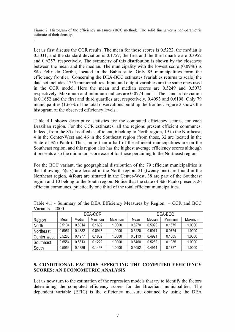
Figure 2. Histogram of the efficiency measures (BCC method). The solid line gives a non-parametric estimate of their density. . Let us first discuss the CCR results. The mean for those scores is 0.5222, the median is 0.5031, and the standard deviation is 0.1757; the first and the third quartile are 0.3952 and 0.6257, respectively. The symmetry of this distribution is shown by the closeness between the mean and the median. The municipality with the lowest score (0.0946) is São Félix do Coribe, located in the Bahia state. Only 85 municipalities form the efficiency frontier. Concerning the DEA-BCC estimates (variables returns to scale) the data set includes 4755 municipalities. Input and output variables are the same ones used in the CCR model. Here the mean and median scores are 0.5249 and 0.5073 respectively. Maximum and minimum indices are 0.0774 and 1. The standard deviation is 0.1652 and the first and third quartiles are, respectively, 0.4093 and 0.6198. Only 79 municipalities (1.66% of the total observations build up the frontier. Figure 2 shows the histogram of the observed efficiency levels.. Table 4.1 shows descriptive statistics for the computed efficiency scores, for each Brazilian region. For the CCR estimates, all the regions present efficient communes. Indeed, from the 85 classified as efficient, 6 belong to North region, 19 to the Northeast, 4 in the Center-West and 46 in the Southeast region (from those, 32 are located in the State of São Paulo). Thus, more than a half of the efficient municipalities are on the Southeast region, and this region also has the highest average efficiency scores although it presents also the minimum score except for those pertaining to the Northeast region. For the BCC variant, the geographical distribution of the 79 efficient municipalities is the following: 6(six) are located in the North region, 21 (twenty one) are found in the Northeast region, 4(four) are situated in the Center-West, 38 are part of the Southeast region and 10 belong to the South region. Notice that the state of São Paulo presents 26 efficient communes, practically one third of the total efficient municipalities. Table 4.1 - Summary of the DEA Efficiency Measures by Region – CCR and BCC Variants – 2000 DEA-CCR DEA-BCC Region Mean Median Minimum Maximum Mean Median Minimum Maximum North 0.5134 0.5014 0.1602 1.0000 0.5270 0.5090 0.1675 1.0000 Northeast 0.5051 0.4882 0.0947 1.0000 0.5220 0.5071 0.0774 1.0000 Center-west 0.5266 0.4977 0.1862 1.0000 0.5113 0.4921 0.1605 1.0000 Southeast 0.5554 0.5313 0.1222 1.0000 0.5460 0.5282 0.1085 1.0000 South 0.5056 0.4886 0.1497 1.0000 0.5052 0.4911 0.1727 1.0000 5. CONDITIONAL FACTORS AFFECTING THE COMPUTED EFFICIENCY SCORES: AN ECONOMETRIC ANALYSIS Let us now turn to the estimation of the regression models that try to identify the factors determining the computed efficiency scores for the Brazilian municipalities. The dependent variable (EFIC) is the efficiency measure obtained by using the DEA

7

method. The explicative variables describe relevant characteristics of the municipalities considered. 5.1 The Econometric Model Let n be the number of municipalities, )',...,( 1 nθθθ = the vector of efficiency scores, X a matrix of dimension n x p, containing the municipality characteristics, β a p-dimensional vector of unknown parameters and e u a n-dimensional vector of random errors. Thus, we can write a regression model as

.,...,1,);( ntuxf ttt =+= βθ Here, denotes the p-dimensional vector of the characteristics of the t-th municipality. As we do not have a priori information about the functional form of f, we suppose linearity,

tx

.uX += βθ

As the efficiency scores are restricted to assume values within the standard unitary interval, ( 10 ≤<θ ), the OLS estimator will be inconsistent in the sense that it will not converge on probability to the true unknown parameter. Yet, it has been shown in the literature that the use of log( )θ as dependent variable leads to consistent and unbiased OLS estimates if the computed scores assume only strictly positive values. Furthermore, when the dependent variable is censored, as is the case with our scores, the OLS estimator of a linear regression will not be consistent and such inconsistency worsens with the proportion of the censored observation in the sample. A proof of this result, under some regularity conditions is given in Greene (1981). This implies that the problem of non-consistency will not be serious when the number of censored observation is small. Censored observations may be appropriated tackled by the Tobit model. In this model, parameters are usually estimated by using the maximum likelihood method (ML) under the suppositions of normality and homoskedasticity. Notice that the absence of normality as well as the presence of heteroskedasticity lead to inconsistent ML estimates. Another important aspect of modeling in classical or Tobit regression, in our particular case, is the possibility of existence of spatial effects leading to the existence of some functional relationship between the municipal efficiency structures in two distinct points in the considered space. The smaller the area where those points are located, the higher is the probability of the existence of the geographical correlation. Anselin (1988) proposed the following model to explicitly consider the spatial dependency:

uXWy ++= βρθ , with u ,eWu += λ where W is a n x n matrix that controls the existence of a neighborhood relationship among localities. Here, the parameter ρ measures the spatial correlation that if present, implies that the computed efficiency score of a given municipality is directly affected by the scores of its neighbors. The parameterλ captures the spatial correlation between the errors and e stands for a new error term.4

8

Here we will use two forms for the W matrix: firstly, the element (i,j) from W will be one if the municipalities i and j are neighbors and zero on the opposite case. In this case neighborhood will be defined as the geographical distance equal or inferior to 50 kilometers; secondly, the element (i,j) from W will be equal to the distance between the municipalities i and j divided by the maximum distance encountered; hence, we have a measure between zero and one for all peer of localities and not only a binary measure of neighborhood. As the municipalities differ significantly on various aspects, it is reasonable to expect that their associated errors also present distinct variances. Thus, when estimating the parameters we should take into account the existence of heteroskedasticity. Hence, the unknown parameters will be estimated by using the linear regression model instead of the Tobit model. The reasons of such choice are listed below. 1. Contrary to the Tobit model, the linear model does not require the supposition of

normality that could be restrictive assumption as we have no information about this issue.

2. The OLS estimates proved to be unbiased and consistent even if the heteroskedasticity is neglected whereas this is not true for the ML estimators of the Tobit model.

3. It is possible to obtain an estimate for the covariance matrix associated with the OLS estimator β that is consistent under the homoskedasticity and the heteroskedasticity hypotheses (see below); hence, we can make hypothesis tests that are asymptotically valid, independently of the structure of the variance of errors and of its distribution. These convenient properties do not apply to the Tobit estimators.

4. The proportion of the censored observation on the whole sample is very low (around 1.8%).

As for the covariance matrix of the OLS estimator of the parameter β (point 3 above), different estimators can be find in the specialized literature. White (1980) proposed a consistent estimator, commonly used in empirical modeling and known as HC0. This estimator is given by

,)'(ˆ')'( 11 −− Ω XXXXXX

where is a n x n diagonal matrix, containing in its principal diagonal the square of the OLS residuals. However, Monte Carlo simulations studies have shown that this estimator tends to produce tests that are too liberal in the sense that their true size is superior to the significance levels of the tests (See Cribari-Neto (2003), Long e Ervin (2000) e MacKinnon e White (1985)).

Ω

Alternative estimators to the White test were proposed. Among them we find the HC3, where the t-th element of the diagonal de Ω is not , but , where is the t-th element of the diagonal of the “hat matrix”, . As h gives a degree of leverage associated to the observation t, this estimator includes a correction for the distinct leverage levels. Simulation results have shown that this estimator leads

2ˆtuH

22 )1/(ˆ tt hu −

')'( 1 XXX −th

X= t

9

to more precise inferences than the White estimator (HC0) and its other variants (see Davidson e MacKinnon (1993) e Long e Ervin (2000)). Cribari-Neto (2003) proposed the estimator HC4, where the square of the t-th residual in matrix Ω is divided by

, where ˆ

tth δ)1( − )/,4min( pnhtt =δ , instead of using ( . Numerical results show

that quasi-t tests, whose statistics use this estimator typically, present lower size distortions when compared with alternative tests. Indeed, those results show that the performance of the test based on HC4 is similar to the ones based on double bootstrap schemes that are highly computational intensive.

2)1 th−

5.2 Estimation Results: The Linear Model

Let us now discuss the estimations. The dependent variables correspond to the logarithm natural of the efficiency scores for 4755 Brazilian municipalities computed by using the DEA-CCR and the DEA-BCC variants. In this first version we try to include most of the municipalities characteristics except the ones that were almost certain multicollinear. Some of these variables are dummy variables that assume value one if the related characteristic is present and zero in its absence. The second model was estimated considering only the regressors that were significant in the first version. In both models, the results were obtained by using the linear regression model, the parameters were estimated by ordinary least squares and their standard errors were estimated by using the HC3 estimator above described. Table 5. presents the explicative variables as well as the econometric results for two models for each DEA variant. To facilitate the discussion we will group the results by category of explicative variable. Spatial and localization effects: Looking at table 5.1, we first notice the relevance of the neighborhood effect in the spatial distribution of the efficiency scores. Indeed, in the four models tested, we find a positive spatial correlation indicating that higher efficiency levels tend to spread out, at least, partially, to the surrounding localities, in a kind of “demonstration effect”. As for the location aspects, there is a clear efficiency premium for state capitals, as those cities tend to present higher scores when compared with other localities with similar characteristics. The same effect could not be found for the metropolitan areas indicating that this somehow “privileged” location does not influence the computed efficiency. Finally, as expected, the municipalities located in the draught areas (Polígono da Seca), are likely to be less efficient than their counterparts in more clement areas thus showing that those cities, hit by adverse climatic conditions, have more difficulty of providing the required public services to its population. Socio-economic impacts: The income level and the poverty proxy (variables E3 and E4, respectively) were significant only when the efficiency scores were estimated by using the DEA-BCC variant; surprisingly, for both variables, the sign of the effects were reversed. So, the fact that a municipality is relatively impoverished does not implies per se a poor resource management. In spite of being characterized by a low-income population, those communes may rationally use their resources thus overcoming its disadvantage background. Furthermore, among the very poor municipalities, those which participate into the Alvorada Project, when we control for other factors, tend to be more efficient; probably, the monitoring required by this program contributes to increase the efficient use of scarce resources, signaling that a better management could be a by-product of the Alvorada Project.

10

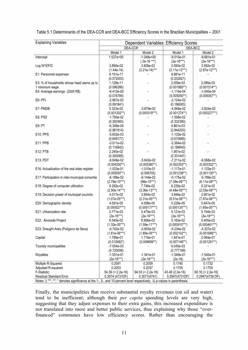
Table 5.1 Determinants of the DEA-CCR and DEA-BCC Efficiency Scores in the Brazilian Municipalities – 2001

Dependent Variables: Efficiency Scores DEA-CCR DEA-BCC

Explaining Variables

Model 1 Model 2 Model 1 Model 2 Intercept 1.027e+00

-1.048e+00 ( 2e-16 ***)

-9.515e-01 (2e-16***)

-9.681e-01 (2e-16***)

Log W1EFIC 3.890e-02 (1.44e-14)

3.826e-02 (2.21e-14)***

3.593e-02 (3.11e-12***)

3.592e-02 (2.87e-12***)

E1: Personnel expenses 8.151e-11 (0.572003)

- 9.881e-11 (0.202621)

-

E3: % of households whose head earns up to 1 minimum wage

1.128e-11 (0.096386)

- 2.059e-03 (0.001860**)

2.085e-03 (0.001514**)

E4: Average earnings (2000 R$) -6.412e-05 (0.074784)

- -1.114e-04 (0.005050**)

-1.045e-04 (0.005057**)

E6: PFL -2.867e-02 (0.091841)

- -2.124e-02 (0.186083)

-

E7: PMDB 5.323e-02 (0.001302**)

-3.879e-02 (0.000319***)

-4.948e-02 (0.001274**)

-3.824e-02 (0.000227***)

E8: PSD -1.793e-02 (0.300360)

- -1.558e-02 (0.332390)

-

E9: PT -6.348e-04 (0.981914)

- 4.861e-03 (0.844203)

-

E10: PPS -5.602e-03 (0.849177)

- -1.133e-02 (0.670685)

-

E11: PPB -3.011e-02 (0.116842)

- -2.364e-02 (0.188640)

-

E12: PTB 2.240e-02 (0.300085)

- 1.951e-02 (0.331447)

-

E13: PDT -6.848e-02 (0.004200**)

-5.642e-02 (0.005380**)

-7.211e-02 (0.002353**)

-6.068e-02 (0.003302**)

E16: Actualization of the real state register -1.033e-01 (0.005597**)

-1.010e-01 (0.006705)

-1.117e-01 (0.001238**)

-1.123e-01 (0.001130**)

E17: Participation in inter-municipal consortia -6.188e-02 (2.79e-10***)

-6.144e-02 (98e-10***)

-5.175e-02 (7.39e-08***)

-5.189e-02 (6.11e-08***)

E18: Degree of computer utilization 8.292e-02 (2.50e-14***)

7.746e-02 (3.36e-13***)

6.235e-02 (4.48e-09***)

6.321e-02 (2.53e-09***)

E19: Decision power of municipal councils 4.017e-02 (1.07e-05***)

3.854e-02 (2.31e-05***)

3.946e-02 (6.51e-06***)

3.901e-02 (7.87e-06***)

E20: Demographic density 4.091e-05 (0.000527***)

4.098e-05 (0.000177***)

5.228e-05 (0.000135***)

5.647e-05 (1.65e-05***)

E21: Urbanization rate 5.771e-03 (2e-16***)

5.479e-03 (2e-16***)

5.121e-03 (2e-16***)

5.154e-03 (2e-16***)

E22: Alvorada Project 6.545e-02 (1.32e-05***)

8.906e-02 (1.59e-11***)

5.163e-02 (0.000910***)

5.405e-02 (0.000461***)

E23: Draught Area (Polígono da Seca) -6.742e-02 (1.81e-06***)

-5.855e-02 (1.89e-05***)

-4.234e-02 (0.002102**)

-4.327e-02 (0.001666**)

Capital 1.789e-01 (0.012682*)

1.716e-01 (0.008699**)

1.841e-01 (0.007146**)

2.064e-01 (0.001291**)

Touristy municipalities -7.054e-03 (0.720006)

- 6.045e-03 (0.777199)

-

Royalties -1.551e-01 (2e-16***)

-1.541e-01 (2e-16***)

-1.549e-01 (2e-16)

-1.545e-01 (2e-16***)

Multiple R-Squared: 0.2091 0.2059 0.1745 0.1732 Adjusted R-squared: 0.2053 0.2037 0.1705 0.1705 F-Statistic: 54.39 (< 2.2e-16) 94.53 (< 2.2e-16) 43.49 (2.2e-16) 66.16 (< 2.2e-16) Residual Standard Error 0.3074 (4731DF) 0.3077(4741) 0.2947(4731DF) 0.2947(4739 DF) Notes: i) ***, **, * denotes significance at the 1-, 5-, and 10-percent level respectively; ii) p-values in parenthesis. Finally, the municipalities that receive substantial royalty revenues (on oil and water) tend to be inefficient; although their per capita spending levels are very high, suggesting that they adjust expenses to their extra gains, this increased expenditure is not translated into more and better public services, thus explaining why those “over-financed” communes have low efficiency scores. Rather than encouraging the

11

optimality of resource use, those additional royalties receipts seem instead to contribute to relax fiscal constraints and spread inefficiency. Summarizing, our results clearly show that there is no direct relationship between higher revenues and better life conditions, as measured by the accessibility to public services. Economies of scale indicators: the scale variables included in the analysis were relevant for explaining efficiency in all versions estimated. Both, the demographic density and the urbanization rate had a strong positive effect on the efficiency scores thus corroborating previous insights suggested by the non-parametric analysis described in Section 3. Indeed, the fact that cities with very low-density rates tend to be less efficient is probably due to the presence of local increasing returns to scale prevalent among small municipalities. The scattered population on those cities tends to raise the average costs of public services, thus preventing them from exploiting the economies of scale that characterizes the production of those services, and so they fail to use optimally its resources. On the other hand, higher density rates decrease the costs of the above-mentioned services and hence contribute to increase efficiency. The strong effect of the urbanization rate on efficiency measures (its p–value is inferior to ) also captures the scale effect, as the average costs of local public services on the less inhabited rural areas tend to be higher. Moreover, this variable may catch the fact that human and material administration resources are scarcer in the rural areas thus reducing the efficiency indices for the less urbanized communities

16102 −×

Political impacts: As for the impact of the mayor political party on efficiency, only the coefficients for the PMDB and for the PDT were significant at 5% level, thus indicating that municipalities run by a mayor coming from those parties tend to be more inefficient. This result holds for all tested models, including the ones using quantile regression, and deserve a more careful analysis. For the rest of the political parties, the mayor’s political affiliation does not affect the efficiency scores. Management variables: As for the management variables, surprisingly, we find out an inverse relationship between the efficiency scores and the degree of actualization of the real state register; such a relation is significant in all tested versions. This variable was supposed to be a proxy for a good fiscal administration; yet, our results consistently suggest that even if a mayor is eager to maintain its tax revenues, this not prevent him from neglecting the way it is spent. On the other hand, the inverse relationship between efficiency and participation in inter-municipal consortia may be due to the fact that, ceteris paribus, only the municipalities, which suffer the most from the lack of an adequate scale on the production of public services, thus being likely to present low efficiency scores, have an incentive to join those consortia in an attempt to reduce average costs. There is also a strong positive relationship between the efficiency scores and the degree of computer utilization (p-value: ); such a relationship was expected; indeed, as computer utilization eases administrative tasks, it is a powerful tool on managing practice thus being an indicator of a “superior” and more effective decision-making process. Finally, in all tested models, we found that the higher the power accorded to municipal councils, the better the effectiveness in resource utilization as measured by efficiency indices. This is rather predictably as those councils tend to increase the transparency of the budgeting process hence contributing to a better control of corruption and misuse of local funds.

131036.3 −×

12

Notice also that the test of Koenker (1981) points out to the presence of heteroskedasticity, thus justifying the utilization of robust standard errors. Indeed, the p-value of the null hypothesis of homoskedasticity is , indicating strong evidence against the assumption of constant conditional variances.

1210971.7 −×

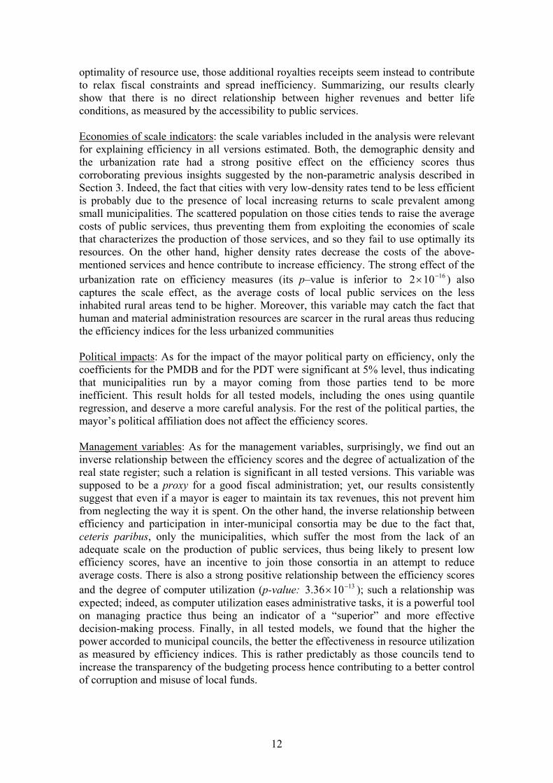
5.3 Quantile Regression Estimators To complement the econometric analysis carried out in the previous sub-section, we will proceed to a more detailed investigation by using quantile regression, introduced by Koenker and Bassett (1978). Just as classical linear regression permits to estimate models for conditional mean functions, quantile regression methods offer a mechanism for estimating models for the conditional median function, and the other conditional quantile functions. This allows us to investigate the impacts of the conditioning variables on the efficiency scores along different efficiency classes. The basic idea is to estimate the τ -th quantile of efficiency conditionally to the different explicative variables, assuming that this quantile may be expressed as a linear predictor based on those conditioning variables. In order to do that, we considered the following conditional quantiles: 0.10 (percentile 10%), 0.25 (quartile inferior), 0.50 (median), 0.75 (quartile superior) e 0.90 (percentile 90%). In each case, we kept the explicative variables that proved to be significant. Results are shown in Table 5.2 (DEA-CCR) and Table 5.3 (DEA- BCC).

Table 5.2: Determinants of the DEA-CCR Efficiency Scores in the Brazilian Municipalities – Quantile Regression – 2001

Dependent variable: DEA-CCR Efficiency Scores by Quantiles Explaining Variables τ = 0,10 τ = 0,25 τ = 0,50 τ = 0,75 τ = 0,90

Intercept -1.38413 (0.00000)

-1.19915 (0.00000)

-1.03893 (0.00000)

-0.92051 (0.00000)

-0.63196 (0.00000)

Log W1EFIC 0.06012 (0.00000)

0.03935 (0.00000)

0.03264 (0.00000)

0.03339 (0.00000)

0.01804 (0.01884)

E7: PMDB -0.04483 (0.01539)

- -0.02938 (0.01728)

-0.03843 (0.00288)

-0.04642 (0.00226)

E13: PDT -0.10112 (0.07923)

-0.07168 (0.00073)

- - -

E16: Actualization of the real state register

-0.28662 (0.00002)

-0.23657 (0.00000)

-0.12799 (0.00001)

- -

E17: Participation in inter-municipal consortia

-0.04769 (0.00891)

-0.06757 (0.00000)

-0.06073 (0.00000)

-0.06839 (0.00000)

-0.06741 (0.00000)

E18: Degree of computer utilization 0.13157 (0.00000)

0.12568 (0.00000)

0.08889 (0.00000)

0.04954 (0.00008)

-

E19: Decision power of municipal councils

0.05059 (0.00310)

0.03215 (0.01022)

0.03131 (0.00169)

0.03839 (0.00068)

0.04619 (0.00042)

E20: Demographic density 0.00005 (0.02141)

0.00003 (0.00000)

0.00004 (0.00937)

0.00004 (0.00247)

0.00006 (0.00216)

E21: Urbanization rate 0.00594 (0.00000)

0.00605 (0.00000)

0.00585 (0.00000)

0.00565 (0.00000)

0.00515 (0.00000)

E22: Alvorada Project 0.09479 (0.00001)

0.11654 (0.00000)

0.09726 (0.00000)

0.08727 (0.00000)

0.04073 (0.02345)

E23:Draught Area (Polígono da Seca) - -0.05178 (0.00832)

-0.04818 (0.00157)

-0.06185 (0.00000)

-0.08570 (0.00002)

Capital - 0.15696 (0.00000)

0.18060 (0.00002)

0.19309 (0.03485)

-

Royalties -0.29870 (0.00000)

-0.18286 (0.00000)

-0.13622 (0.00000)

-0.10543 (0.00000)

-0.10344 (0.00000)

13

Firstly, notice that the geographic influence is present in all the quantiles analyzed; however, this influence is much stronger for the more inefficient municipalities. Remark also that the capital effect does not appear here indicating that, for those communes there is no such effect; this is probably due to the fact that there is only a few capitals and they are not situated in this extremely low range of efficiency. For the two next quantiles (τ = 0,25 and τ = 0, 50), in both, the CCR and the BCC variants, being a state capital improves efficiency, but for very efficient communes this fact no more matters. Finally, for the municipalities standing in the lower efficiency class, their location on the Draught Area (Polígono das Secas) is no more relevant for explaining efficiency, suggesting, that for such cities, other sources of inefficiency predominates over this particular location.

Table 5.3: Determinants of the DEA-BCC Efficiency Scores in the Brazilian Municipalities – Quantile Regression – 2001

Dependent variables: DEA-BCC Efficiency Scores by Quantiles Explicative Variables τ = 0,10 τ = 0,25 τ = 0,50 τ = 0,75 τ = 0,90

Intercept -1.32959 (0.00000)

-1.14491 (0.00000)

-0.91908 (0.00000)

-0.77514 (0.00000)

-0.58300 (0.00000)

Log W1EFIC 0.05939 (0.00000)

0.043301 (0.00000)

0.03079 (0.00000)

0.03009 (0.00000)

0.01042 (0.12964)

E3: % of households whose head earns up to 1 minimum wage

0.00404 (0.00038)

0.00391 (0.00000)

0.00190 (0.00609)

-0.00031 (0.65627)

-0.00073 (0.43679)

E4: Average earnings -0.00005 (0.36421)

-0.00007 (0.13181)

-0.00013 (0.00002)

-0.00017 (0.00023)

-0.00016 (0.00000)

E7: PMDB -0.05472 (0.00348)

-0.03855 (0.00522)

-0.02847 (0.01140)

-0.03585 (0.00205)

-0.04428 (0.00131)

E13: PDT -0.13924 (0.00000)

-0.07225 (0.00156)

-0.04576 (0.05766)

-0.04690 (0.03194)

-0.04162 (0.18252)

E16: Actualization of the real state register

-0.25519 (0.00002)

-0.23130 (0.00000)

-0.15254 (0.00000)

-0.03686 (0.27449)

0.02290 (0.62725)

E17: Participation in inter-municipal consortia

-0.04298 (0.00810)

-0.05681 (0.00002)

-0.06016 (0.00000)

-0.06195 (0.00000)

-0.04865 (0.00007)

E18: Degree of computer utilization 0.09712 (0.00000)

0.11219 (0.00000)

0.07437 (0.00000)

0.03983 (0.00090)

-0.00080 (0.95586)

E19: Decision power of municipal councils

0.04568 (0.00262)

0.04063 (0.00100)

0.03214 (0.00060)

0.04384 (0.00002)

0.04842 (0.00003)

E20: Demographic density 0.00005 (0.00000)

0.00003 (0.00000)

0.00007 (0.00000)

0.00006 (0.00208)

0.00006 (0.00000)

E21: Urbanization rate 0.00515 (0.00000)

0.00563 (0.00000)

0.00545 (0.00000)

0.00530 (0.00000)

0.00511 (0.00000)

E22: Alvorada Project 0.06627 (0.00545)

0.07644 (0.00026)

0.05019 (0.00200)

0.05995 (0.00051)

0.03542 (0.08215)

E23:Draught Area (Polígono da Seca) -0.01010 (0.65653)

-0.05159 (0.00565)

-0.03456 (0.02235)

-0.05202 (0.00048)

-0.06489 (0.00117)

Capital 0.22598 (0.00746)

0.20778 (0.00000)

0.17652 (0.00000)

0.22153 (0.00287)

0.19794 (0.00428)

Royalties -0.27136 (0.00000)

-0.17746 (0.00000)

-0.13238 (0.00000)

-0.10369 (0.00000)

-0.10160 (0.00017)

As to the impact of socio-economic factors on efficiency, the quantile regression analysis, using the BCC version, is much more clarifying than the previous ones. Indeed, for the inefficient municipalities, it shows clearly that a higher proportion of low-income population contributes to increase efficiency scores, although this effect is

14

rather small. The underlying reason is probably the fact that those communes usually benefit from a bunch of social programs that are closely monitored; thus, with them comes a pressure for more rational resource utilization. Regarding the impact of average income on efficiency, the BCC results confirms our previous finding that is has a negative effect on efficiency grounds. Finally, as for the royalties’ receipts, the quantile regression estimates confirm our anterior results according to which receivers of substantial royalty revenues are more inefficient. The new point here is the fact that this impact gets smaller when efficiency increases, being particularly damaging for extreme inefficient communes. This may indicate that they have no managerial capabilities to handle usefully those additional resources. According to those disaggregated results, the influence of politics on efficiency is similar to the one previously found. Except, for two parties, PDT and PMDB, the mayor’s political affiliation does not affect the efficiency scores. However, here, the estimated negative effect for those parties are not very significant; particularly, in the case of PDT, the negative effect is present only for the first two cases (τ = 0,10 and τ = 0, 25). Moreover, our results reveal that the impact of the degree of computer utilization increases along the different conditional quantile. Indeed, the estimated coefficients corresponding to this variable for the conditional quantiles 75.0.50.0,25.0,10.0=τ are 0.132, 0.126, 0.089 and 0.050, respectively, thus indicating the existence of diminishing marginal benefits for computer. Due to widespread use of computer equipment in the highly efficient municipalities, most likely, computer use is no longer a proxy for “superior” management. Contrary to the aggregate analysis, where the negative effect of the degree of actualization of the real state register on efficiency results was clearly verified, in the quantile regression analysis, this is true only for the more inefficient municipalities; On the other hand, we thought that the inverse relationship between efficiency and participation in inter-municipal consortia was caused by diseconomies of scale prevalent among inefficient municipalities. Yet, here the results shows that, except for the two extremes quantiles (τ = 0,10 and τ = 0, 90), this effect is quite widespread, thus suggesting, that even relatively efficient municipalities cannot reach the optimum size for hospitals, for instance, and thus seeks to join those consortia in an attempt to reduce costs. Notice also that for the lower classes of efficiency, the decision power of the municipal councils was less significant, thus meaning less control on the use of public resources once more attesting those cities lack of managerial capabilities. Last but not least as in the preceding analysis, the scale variables – demographic density and urbanization rate – have positive and significant effect upon efficiency. 5.4 Alternative Results by Using Linear Regression To conclude our investigation, we will examine a data set where the municipalities do not have any vicinity relationship. This new sample was build up by selecting all the capitals and other cities randomly as long as no peers of municipality were at an inferior distance of 50 (fifty) kilometers. We hope, this way, to eliminate all the spatial correlation. The new data set includes 768 municipalities whose average efficiency is 0.520, its median is 0.500, the standard deviation is 0.1795, and finally the minimum efficiency is 0.0947. With the DEA-CCR variant, roughly 2% of the communes turn out

15

to be efficient. As before, in the econometric analysis, we first fitted a model including most of the conditional variables (model 1) and after, in model 2, we only considered the ones that were significant in the first model. Results are shown in Table 5.4.

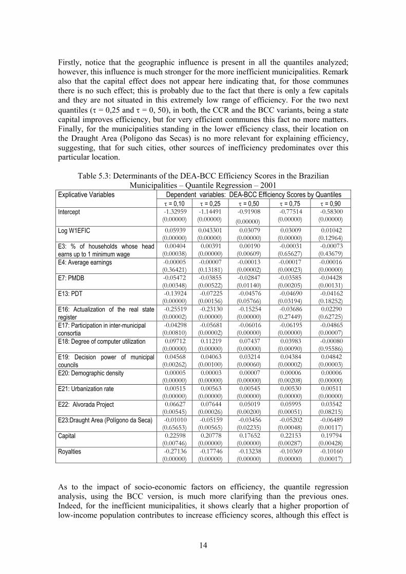
Table 5.4: Determinants of the DEA-CCR Efficiency Scores for Selected Brazilian Municipalities – 2001

Explicative Variables Model 1 Model 2 Coefficients p-value Coefficients p-value Intercept -7.795e-01 2.71e-09*** -0.719982 9.23e-10*** E1: Personnel expenses 2.621e-10 0.169141 - - E3: % of households whose head earns up to 1 minimum wage

3.196e-03 0.070036 - -

E4: Average earnings -1.307e04 0.132175 - - E6: PFL -7.254e-02 0.111793 - - E7: PMDB -5.010e-02 0.267346 - - E8: PSDB -3.212e02 0.488912 - - E9: PT -3.170e-02 0.656756 - - E10: PPS -1.499e-01 0.030415* -0.108346 0.0726 E11: PPB -5.698e-02 0.293851 - - E12: PTB -5.456e-03 0.925034 - - E13: PDT -8.125e-02 0.196863 - - E16: Actualization of the real state register -2.297e-01 0.045026* -0.216372 0.0560 E17: Participation in inter-municipal consortia -2.893e-02 0.292917 - - E18: Degree of computer utilization 1.120e-01 0.000111*** 0.057208 0.0330* E19: Decision power of municipal councils 5.194e-02 0.038016* 0.046399 0.0645 E20: Demographic density 1.937e-06 0.955813 - - E21: Urbanization rate 4.082e-03 1.19e-08*** 0.002582 3.28e-05*** E22: Alvorada Project 6.570e-02 0.066931 - - E23: Draught Area (Polígono da Seca) -3.786e-02 0.300383 - - Capital 3.304e-01 0.003270** 0.354782 2.42e-06*** Metropolitan areas 7.922e-03 0.896420 - - Royalties -1.223e-01 0.029736* -0.079908 0.1431 Multiple R-Squared: 0.1505 - 0.1103 - Adjusted R-squared: 0.1254 - 0.1021 - F-Statistic: 5.999 (4.714e-16) - 13.46 (2.2e-16) - Residual Standard Error 0.3364 (745 DF) - 0.3408(760) - Notes: i) ***, **, * denotes significance at the 1-, 5-, and 10-percent level respectively;

As a general remark let us notice that in this new sample, the main results are quite similar to the ones obtained when the whole set was used. Yet, we observe a few noteworthy differences. Firstly, the density demographic, a variable that stands for economies of scale is no more significant. Secondly, the royalty receipts was not significant in this sample, in model 2, at the nominal level of 10%. In order to investigate this point, we estimate quantile regressions for the conditional quantiles: 90.0,75.0,50.0,25.0,10.0=τ . We found out that the negative impact of royalties on efficiency is statistically significant only for the superior quartile, 75.0=τ . This means that, for this sample, the results contradict the ones obtained when applying the both the BCC and the CCR methods on the whole set. Remember that in both models, clearly, the negative impact of royalty receipts decreased with the efficiency level. Lastly, the impact of the mayor’s affiliation party on efficiency changes a great deal as now neither the PMDB nor the PDT have the negative influence they used to have on the previous estimates. Rather, the PPS appears now as the only political party negatively affecting efficiency.

16

6. CONCLUDING REMARKS In this paper we have firstly estimated the DEA CCR and BCC technical efficiency scores for 4796 Brazilian municipalities by applying a method, which combines Bootstrap and Jackknife resampling techniques to eliminate the effect of outliers and measurement errors in the data set. The computed efficiency scores, as well as their rank, proved to be very robust for both variants, thus increasing the credibility of the estimated frontiers. As the estimated efficiency scores are affected by exogenous characteristics, which were not taken into account in our DEA calculations, we included those factors in our analysis. Hence, we used techniques of spatial econometrics and quantile regressions to investigate the way those excluded variables could influence the computed scores. Our econometric results proved to be very robust to the non-parametric variants utilized to calculate the dependent variable. The estimated coefficients were also very stable when faced to variations on econometric specifications, techniques used and sample modifications. As we would expect, the spatial effect was consistently significant, thus showing that such an effect could not be ignored when dealing with municipal data. Also, being a state capital increases efficiency but the same is not true for municipalities located in metropolitan areas. In addition, as expected, the communes located in the draught areas (Polígono das Secas), tend to be more inefficient than their equivalents in more clement areas showing that those cities, hit by adverse climatic conditions, have more difficulties to offer an adequate supply of public services. The scale variables (demographic density and urbanization rate) played also an important role in explaining the efficiency scores thus corroborating our previous insight that the recent proliferation of small municipalities, in Brazil, does not lead to an efficient use of public resources. Their small size prevents these communes to benefit from the economies of scale inherent to the production of publics services and so, they tend to operate with higher average costs thus bringing about a considerable waste of resources. As for the management variables, on the other hand, the inverse relationship between efficiency and participation in inter-municipal consortia may be due to the fact that, ceteris paribus, only the municipalities, which operate on a scale much below the optimum, thus being likely to present low efficiency scores, have an incentive to join those consortia in an attempt to reduce average costs and increase efficiency. There is also a strong positive relationship between the efficiency scores and the degree of computer utilization. Such a relationship was expected; indeed, as computer utilization eases administrative tasks, it is a powerful tool on managing practice thus being an indicator of a “superior” and more effective decision-making process. Our quantile regression estimates suggest that the more inefficient the municipality, the higher the benefits derived from computer utilization. We find out an inverse relationship between the efficiency scores and the degree of actualization of the real state register; such a relation is significant in all models tested. Finally, in all tested models, we found that the higher the power accorded to municipal councils, the better the effectiveness in resource utilization as measured by efficiency indices. This is rather predictably as those councils tend to increase the transparency of the budgeting process hence contributing to a better control of corruption and misuse of local funds.

17

Also, the socio economic variables such as the municipality mean income level and the poverty proxy were significant only when the efficiency scores were estimated by means of the DEA-BCC variant; surprisingly, for both variables, the sign of the effects were reversed. Thus our results seem to imply that poor cities, by wisely using their resources, may overcome its initial environmental disadvantages. Furthermore, among the very poor municipalities, those participating in the Alvorada Project tend to be more efficient indicating that a better management could be a by-product of this program. Finally, the municipalities that receive substantial royalty revenues tend to be inefficient suggesting that this increased gains rather than encouraging the optimality of resource use, seem instead to contribute to relax fiscal constraints and spread inefficiency. The natural extension of our current investigation would be to use the econometric results to separate the effects of the exogenous factors from those related to the technical aspects of the productive process, in order to obtain a “pure” measure of technical efficiency for the Brazilian municipalities. 7. REFERENCES Anselin, L. (1988). Spatial Econometrics: Methods and Models. Dordrecht: Kluwer. Banker, R. D., Charnes, A and Cooper, W.W. (1984) “Some Models for Estimating Technical and Scale Efficiencies in Data Envelopment Analysis.” Management Science 30: 1078-1092. Banker, R. D and Gifford, J.L. (1988) “A Relative Efficiency Method for the Evaluation of Public Health Nurse Productivity.” Mimeo. Banker, R. J. and Morey, R. C. (1996) “Efficiency Analysis for Exogenously Fixed Inputs and Outputs.” Operation Research 34: 513-521. Charnes, A., Cooper, W.W. and Rhodes, E. (1978) “Measuring Efficiency of Decision Making Units.” European Journal of Operational Research 1:429-44. Cribari-Neto, F. (2003) ”Asymptotic Inference Under Heteroskedasticity of Unknown Form.” Computational Statistics and Data Analysis, forthcoming. Cribari, F and Zarkos, S. “That Voodoo That You Do So Well: Leverage Adjusted Weighted Bootstrap Methods”, preprint. Davidson, R. and MacKinnon, J.G. (1993) Estimation and Inference in Econometrics. New York: Oxford University Press. Ericsson, N. (1991) Lectures in Monte Carlo Methodology: Theory and Practice. 4a Escola de Séries Temporais e Econometria, Rio de Janeiro, RJ. Färe, R., Grosskpof, S. and Lovell, C. K. (1985) The Measurement of Efficiency of Production. Boston: Kluwer-Nijhoff Publishing. Färe, R., Grosskpof, S. and Lovell, C. K. (1994) Production Frontiers. Cambridge University Press. Farrell, M. J. (1957) “The Measurement of Productive Efficiency.” Journal of the Royal Statistical Society Series A 120: 253-281. Gillen, D. and Lall, A (1997) “Developing Measures of Airport Productivity and Performance: An Application of Data Envelopment Analysis. Greene, W.H. (1981) “On the Asymptotic Bias of the Ordinary Least Squares Estimator of the Tobit Model.” Econometrica 49: 505-513. Kalirajan, K. P. (1990) “On Measuring Economic Efficiency.” Journal of Applied Econometrics 5: 75-85. Koenker, R. (1981). “A Note on Studentizing a Test for Heteroskedasticity.” Journal of Econometrics, 17, 107-112.

18

19

Koenker, R. and Bassett, G. (1978). “Regression Quantiles.” Econometrica 46: 33-50. Long, J.S. and Ervin, L.H. (2000) “Using Heteroscedasticity Consistent Standard Errors in the Linear Regression Model.” The American Statistician 54: 217-224. Lovell, C. A K., Walters, L.C. and Wood, L.L. (1994) “Stratified Models of Education Production Using DEA and Regression Analysis.” In Charnes, A, Cooper, W.W, A Y. MacKinnon, J.G. and White, H. (1985) “Some Heteroskedasticity-Consistent Covariance Matrix Estimators with Improved Finite-Sample Properties.” Journal of Econometrics 29: 305-325. McCarty, T. and Yaisawarng (1993) “Technical Efficiency in New Jersey School Districts.” In Fried, H. O, Lovell, C.A K. and Schmidt, S. S. eds., The Measurement of Productive Efficiency. Oxford: Oxford University Press. Sampaio de Sousa, M. C. e Ramos de Souza, F. (1999a) “Measuring Public Spending Efficiency in Brazilian Municipalities: A Non Parametric Approach” in Westermann, G., Ed., Data Envelopment Analysis in the Service Sector. Wiesbaden: DUV, Gabler, pp. 237-267. Sampaio de Sousa, M. C. e Ramos de Souza, F. (1999b) Eficiência Técnica e Retornos de Escala na Produção de Serviços Públicos Municipais.” Revista Brasileira de Economia 53: 433-461. Seaver, B. L. and Triantis, K. P. (1989). "The Implications of Using Messy Data to Estimate Production-frontier-based Technical Efficiency Measures." Journal of Business and Economic Statistics 7: 49-59 Smith, V. K. (1973) Monte Carlo Methods: Role for Econometrics. Lexington: Lexington Books. Stosic, B. and Sampaio de Sousa, M.C. (2003) “Jackstrapping Dea Scores For Robust Efficiency Measurement.” Séries Texto para Discussão N° 291, Universidade de Brasília. Tobin, J. (1958) “Estimation of Relationship for Limited Dependent Variable.” Econometrica 26: 24-36. Yu, C. (1998), “The Effects of Exogenous Variables in Efficiency Measurement – A Monte Carlo Study.” European Journal of Operational Research 105: 569-580. White, H. (1980). “A Heteroskedasticity-Consistent Covariance Matrix Estimator and a Direct Test for Heteroskedasticity.” Econometrica 48, 817-838. Wilson, P. (1993) “Detecting Influential Observations in Data Envelopment Analysis.” Journal of Productivity Analysis 6: 27-45. Wilson, P. (1995) “Detecting Influential Observations in Deterministic Non-Parametric frontiers models.” Journal of Business and Economic Statistics 11: 319-323. NOTES

1 See Charnes, Cooper, and Rhodes (1978), Banker, Charnes, and Cooper (1984), Färe, Grosskpof, and Lovell, (1985, 1994). 2 For a more detailed analysis, see Färe, Grosskpof, and Lovell, (1994). 3The reason why this happens lies on the flourishing creation of new municipalities in Brazil. Indeed, some municipalities, although legally created, have not yet being dismembered from the mother-commune. As a result, they do not report output indicators. In addition, null values for current expenses may be also explained by the fact that the data have not yet been reported by the STN (National Treasure Secretary). 4 Notice that there is no direct interest in the estimation of λ and ρ.