8

Ultrasonic Thruster

Alfred C. H. Tan and Franz S. Hover Massachusetts Institute of Technology

United States of America

1. Introduction

Acoustic streaming refers to the bulk net flow of fluid generated as a result of intense, free-

field ultrasound. This phenomenon, also known as ‘quartz wind’ or ‘sonic wind’, is induced

by a loss in mean momentum flux due to sound absorption in the fluid medium, leading to

a net flow along the transducer axial direction. The transmission of intense sound energy

into the fluid is also associated with a resultant force acting on the transducer surface. This

resultant “backthrust” can be exploited in underwater vehicles for propulsion or

maneuvering purposes. We refer to the device as ultrasonic thruster (UST), shown in Fig. 1,

and define it as an ultrasonic transducer made from piezoelectric material, excited by an

alternating high-voltage source in the megahertz. We provide a general comparison

between various propulsion technologies in Table 1.

Fig. 1. An ultrasonic thrusters (UST) directing a jet through the free water surface.

The UST we describe is being considered as an alternative small-scale propulsor for

underwater robotic devices and systems, because it has no moving parts beyond its

membrane and can be mounted flushed with the body of the watercraft. At a sound level of

132dB (re 1Pa) (Panchal, Takahashi, & Avery, 1995; Tan & Tanaka, 2006), it is destructive to

biofouling and could perform self-cleaning under prolonged water submersion. These

novelties in low maintenance and design robustness, coupled with low cost commercially

off-the-shelf (COTS) transducers, are attributes which are not found in rotary or biomimetic

propulsors of today. For a small transducer diameter of 1cm, thrust generated is in the order

of tens of milli-newtons (mN), suitable for systems operating at low Reynolds numbers.

Jet

UltraSonicThruster

(UST)

www.intechopen.com

Ultrasonic Waves

148

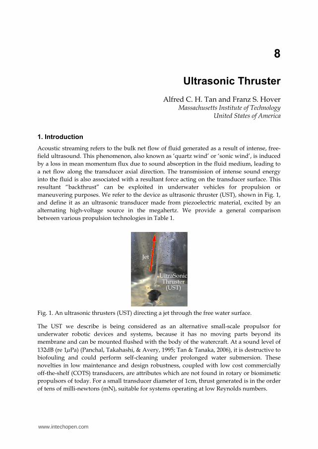
Propulsors Advantages Disadvantages

Fixed-pitch propeller Very mature technology; cost effective

Load- and speed-dependent performance

Podded drive Maneuverability; reduced impact on vessel internal layout; noise isolation

High bearing loads; costly and complex

Ducted propeller High efficiency; directional stability; robustness against line fouling

May be inefficient at off design conditions

Controllable-pitch propeller High efficiency at different advance speeds and loadings

Complex actuation system and maintenance

Waterjet Efficient at high vessel speeds; suitable for shallow water

Poor performance at low speeds; vulnerable to ingested debris

Cycloidal propeller Low-speed maneuverability Complex mechanical structure and maintenance

Biomimetic – body/caudal fin (BCF) locomotion

Efficient and maneuverable at many speeds; quiet

Complex physical design

Biomimetic – Median and/or paired fin (MPF) locomotion

High maneuverability at low speeds; quiet

Complex physical design

Ultrasonic thruster (this work)

Very small size; no moving parts; short-range acoustic communication

Poor propulsive efficiency; requires a high-voltage supply

Table 1. Broad comparison of propulsor technologies (Carlton, 2007; Sfakiotakis, Lane, & Davies, 1999; Tan & Hover, 2009).

At the same time, large-scale collaborative swarm of small “microrobots” or “pods” systems

are also gaining more interest in terms of low cost and practical operation. Small clusters of

exploratory underwater vehicles could also acquire true flexibility in formation morphing,

and wide spatial/temporal coverage in search-survey work (Trimmer & Jebens, 1989). More

importantly, small water submersible is valuable in cluttered or confined environments such

as inside a piping network or complex underwater structures (Egeskov, Bech, Bowley, &

Aage, 1995). Naval reconnaissance missions could involve the deployment of clusters of

expendable (even biodegradable) small underwater robots for hazardous/security missions

such as mine-hunting or surveillance mapping (Doty et al., 1998).

In the following sections, we examine the theoretical background of the UST thrust

generation, introduce scaled parameters for comparison between various UST devices found

in the literature, examine its transit efficiency, identify some thermal anomalies, and discuss

some of the UST design considerations. A detailed construction of the UST will be outlined

with underlying insights to materials selection and design principles. For practical

demonstration, we have also built a small underwater vehicle named Huygens, to establish a

miniaturized platform for supporting multi-objectives subsea tasks. The main focus will be

exclusively on the transducer-only testing (without nozzle appendages) for thrust and wake

characterization as these are fundamentals toward understanding the UST technology. Prior

www.intechopen.com

Ultrasonic Thruster

149

works on thrust by ultrasonic means can be found in (Allison, Springer, & Van Dam, 2008;

Nobunaga, 2004; Wang et al., 2011; Yu & Kim, 2004); we review and expand upon these. We

have also made a comparison among these UST technologies, and provide some insights

into some of the design parameters of ultrasonic propulsion.

2. Underwater Ultrasonic Thruster (UST)

The UST is made from a membrane actuator mounted in a specially designed waterproof

housing, excited by an electrical source at ultrasonic frequency; the UST is generally applied

underwater to generate thrust. For this work, the actuator is made of a thin, circular

piezoelectric plate. We establish some fundamental concepts of the UST physics leading to

thrust as experienced on the transducer surface, and its resulting jet of acoustic streaming

into the farfield. Several nomenclatures are defined and used to describe the experimental

results in the preceding sections.

2.1 Thrust generation

As described in the introduction, there are some prior works on the UST found in the

literature. The experimental model used in those examples varies in shapes and sizes, and in

the following, we provide a basis of comparison among them in terms of thrust density and

electrical power density between each UST design. As an introduction, we refer to the

mathematical treatment of thrust and acoustic power generation in Eqs. (1) to (4) as

originally proposed by (Allison, et al., 2008), and relates thrust to the transducer voltage

supplied, E, a parameter reported in most UST-related studies.

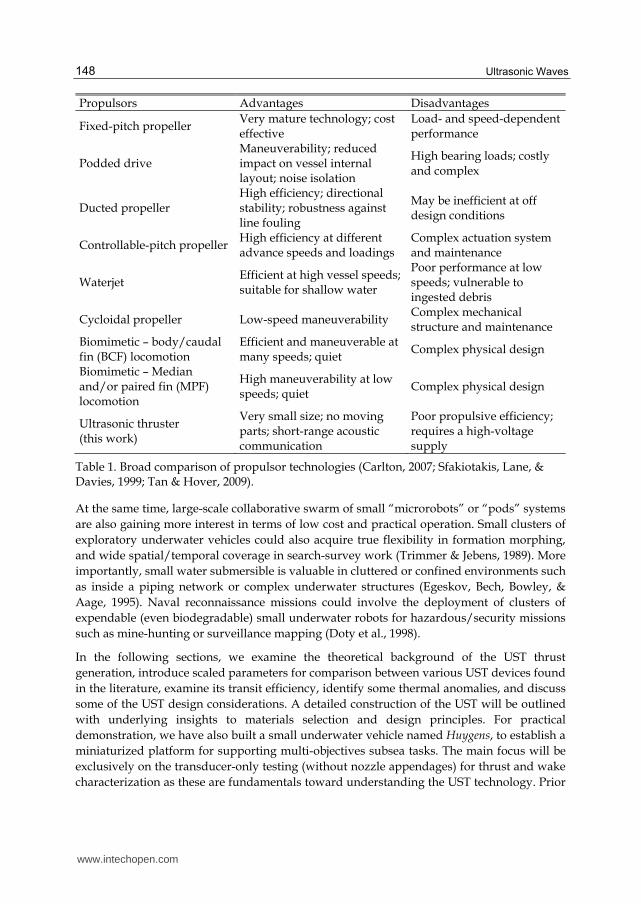
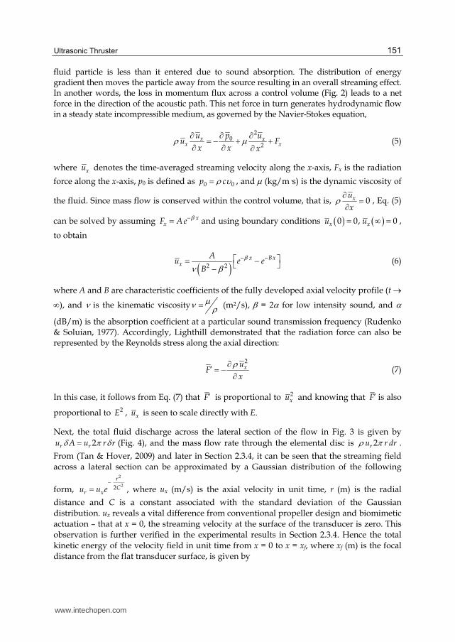
Fig. 2. An elemental control volume in the far-field; the elevation angle, azimuth angle and

distance from the center of transducer are , , and s respectively.

In Fig. 2, several variables for the transducer and the acoustic field are introduced. The

acoustic energy transmits to the right semi-hemisphere, propagating perpendicularly

through an elemental cross-sectional surface area 2 sindS s d d of a control volume 2 sindS s d d ds . According to (Allison, et al., 2008), thrust experienced on the surface of

the transducer is expressed as

2a

S

ds

s dsin s d

x

x’

www.intechopen.com

Ultrasonic Waves

150

1

212 2

0

sin

sino

J kaT a d

(1)

where (kg/m3), o (m/s), a (m), k, , and J1() denote the fluid density, transducer surface

velocity, radius of the transducer, wavenumber, sound absorption coefficient, and Bessel

function of the first kind, respectively, and we consider 11

3.832sin

ka (Blackstock, 2000) as

the upper limit of the dominant ultrasonic beamwidth.

The relationship between the acoustic power along the transducer axial direction x and the ultrasonic thrust is given by a simple relationship (Allison, et al., 2008)

xcTP (2)

where c (m/s) denotes the sound speed, and relates to the efficiency which will be

elaborated in the next paragraph. As we verify below, this also means the thrust is

considerably lower than would a rotary propulsor operating at the same power level.

At s = 0, this acoustic power radiation is associated with the electrical power consumption

across the transducer. The electrical power would provide an approximation to the acoustic

power loading, which relates to the thrust force, and is reflected in the following

considerations through an efficiency constant, ; (i) electrical power lost across the

transducer is not wholly transferred into the medium; (ii) acoustic loading at the sharp

dominant resonant frequency of the transducer may not be precisely tuned; (iii) it is difficult

to consider the equivalent acoustic load in the lumped circuit impedance; (iv) although the

acoustic power is mainly generated within the narrow ultrasonic beam, some losses also

occur outside the beamwidth.

By relating the thrust production to the root mean square of the transducer voltage

supplied, Erms, it can be equated as

2

RermsE

Tc

(3)

where Re() is the real component of the transducer impedance, and the electrical power,

2

RermsE

P (4)

corresponds to Px at s = 0. This thrust scaling with squared voltage in (3) will be used in

Section 2.3.4.

2.2 Acoustic streaming

Following Lighthill (Lighthill, 1978), acoustic streaming arises because of acoustic energy absorption along the path of propagation in a viscous, dissipative fluid medium. A simple explanation of the mechanism can be thought of as exit momentum flux from each exposed

www.intechopen.com

Ultrasonic Thruster

151

fluid particle is less than it entered due to sound absorption. The distribution of energy gradient then moves the particle away from the source resulting in an overall streaming effect. In another words, the loss in momentum flux across a control volume (Fig. 2) leads to a net force in the direction of the acoustic path. This net force in turn generates hydrodynamic flow in a steady state incompressible medium, as governed by the Navier-Stokes equation,

2

02

x xx x

u p uu F

x x x (5)

where xu denotes the time-averaged streaming velocity along the x-axis, Fx is the radiation

force along the x-axis, p0 is defined as 0 0p c , and (kg/m·s) is the dynamic viscosity of

the fluid. Since mass flow is conserved within the control volume, that is, 0xu

x , Eq. (5)

can be solved by assuming xxF Ae and using boundary conditions 0 0, 0x xu u ,

to obtain

2 2

x Bxx

Au e e

B

(6)

where A and B are characteristic coefficients of the fully developed axial velocity profile (t

), and is the kinematic viscosity (m2/s), = 2 for low intensity sound, and

(dB/m) is the absorption coefficient at a particular sound transmission frequency (Rudenko & Soluian, 1977). Accordingly, Lighthill demonstrated that the radiation force can also be represented by the Reynolds stress along the axial direction:

2xu

Fx

(7)

In this case, it follows from Eq. (7) that F is proportional to 2xu and knowing that F is also

proportional to 2E , xu is seen to scale directly with E.

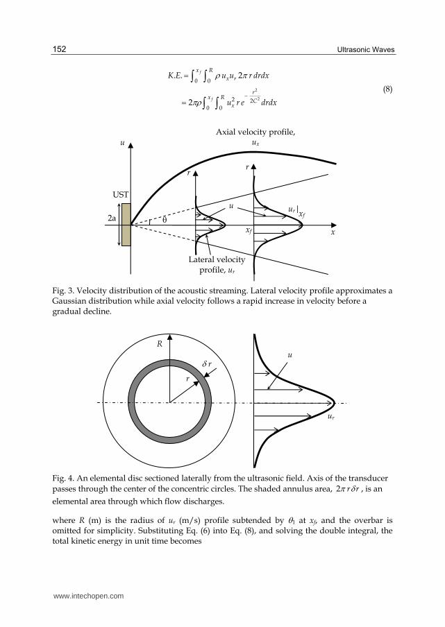
Next, the total fluid discharge across the lateral section of the flow in Fig. 3 is given by

2r ru A u r r (Fig. 4), and the mass flow rate through the elemental disc is 2ru r dr .

From (Tan & Hover, 2009) and later in Section 2.3.4, it can be seen that the streaming field

across a lateral section can be approximated by a Gaussian distribution of the following

form,

2

22

r

Cr xu u e

, where ux (m/s) is the axial velocity in unit time, r (m) is the radial

distance and C is a constant associated with the standard deviation of the Gaussian

distribution. ux reveals a vital difference from conventional propeller design and biomimetic

actuation – that at x = 0, the streaming velocity at the surface of the transducer is zero. This

observation is further verified in the experimental results in Section 2.3.4. Hence the total

kinetic energy of the velocity field in unit time from x = 0 to x = xf, where xf (m) is the focal

distance from the flat transducer surface, is given by

www.intechopen.com

Ultrasonic Waves

152

2

2

0 0

2 20 0

. . 2

2

f

f

x R

x r

rx R

Cx

K E u u r drdx

u r e drdx

(8)

Fig. 3. Velocity distribution of the acoustic streaming. Lateral velocity profile approximates a Gaussian distribution while axial velocity follows a rapid increase in velocity before a gradual decline.

Fig. 4. An elemental disc sectioned laterally from the ultrasonic field. Axis of the transducer

passes through the center of the concentric circles. The shaded annulus area, 2 r r , is an

elemental area through which flow discharges.

where R (m) is the radius of ur (m/s) profile subtended by 1 at xf, and the overbar is omitted for simplicity. Substituting Eq. (6) into Eq. (8), and solving the double integral, the total kinetic energy in unit time becomes

2a x

u

xf

ur|

r r

xf

Axial velocity profile, ux

Lateral velocity profile, ur

u

UST

R

r

r u

ur

www.intechopen.com

Ultrasonic Thruster

153

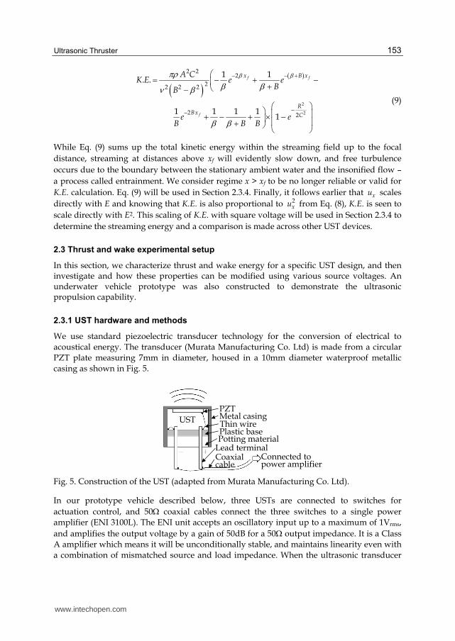
2

2

2 22

22 2 2

2 2

1 1. .

1 1 1 11

f f

f

x B x

RBx C

A CK E e e

BB

e eB B B

(9)

While Eq. (9) sums up the total kinetic energy within the streaming field up to the focal

distance, streaming at distances above xf will evidently slow down, and free turbulence

occurs due to the boundary between the stationary ambient water and the insonified flow –

a process called entrainment. We consider regime x > xf to be no longer reliable or valid for

K.E. calculation. Eq. (9) will be used in Section 2.3.4. Finally, it follows earlier that xu scales

directly with E and knowing that K.E. is also proportional to 2xu from Eq. (8), K.E. is seen to

scale directly with E2. This scaling of K.E. with square voltage will be used in Section 2.3.4 to

determine the streaming energy and a comparison is made across other UST devices.

2.3 Thrust and wake experimental setup

In this section, we characterize thrust and wake energy for a specific UST design, and then investigate and how these properties can be modified using various source voltages. An underwater vehicle prototype was also constructed to demonstrate the ultrasonic propulsion capability.

2.3.1 UST hardware and methods

We use standard piezoelectric transducer technology for the conversion of electrical to

acoustical energy. The transducer (Murata Manufacturing Co. Ltd) is made from a circular

PZT plate measuring 7mm in diameter, housed in a 10mm diameter waterproof metallic

casing as shown in Fig. 5.

Fig. 5. Construction of the UST (adapted from Murata Manufacturing Co. Ltd).

In our prototype vehicle described below, three USTs are connected to switches for

actuation control, and 50 coaxial cables connect the three switches to a single power

amplifier (ENI 3100L). The ENI unit accepts an oscillatory input up to a maximum of 1Vrms,

and amplifies the output voltage by a gain of 50dB for a 50 output impedance. It is a Class

A amplifier which means it will be unconditionally stable, and maintains linearity even with

a combination of mismatched source and load impedance. When the ultrasonic transducer

PZTMetal casingUSTThin wirePlastic basePotting material

Lead terminalConnected to power amplifier

Coaxial cable

www.intechopen.com

Ultrasonic Waves

154

emits intense acoustic energy into the fluid, the thin metal housing provides excellent heat

dissipation. Natural convection and acoustic streaming also aid in carrying away heat from

the transducer surface (Tan & Hover, 2010a).

2.3.2 Thrust force measurement

It is important to develop a reliable underwater thrust measurement method, especially for small thrust magnitudes as is the case of the UST. Most load cells are either non-submersible or could not provide sufficient sensitivity/resolution required at small driving forces. While thrust can also be inferred from acoustic intensity measurement using a hydrophone, it poses some challenges unique to the UST setup, such as membrane cavitation, heating effect, and reading errors averaged from a finite-size hydrophone. Indeed, (Hariharan et al., 2008) reported that acoustic intensity measurements do not perform well, having an error in excess of 20% with experimental data.

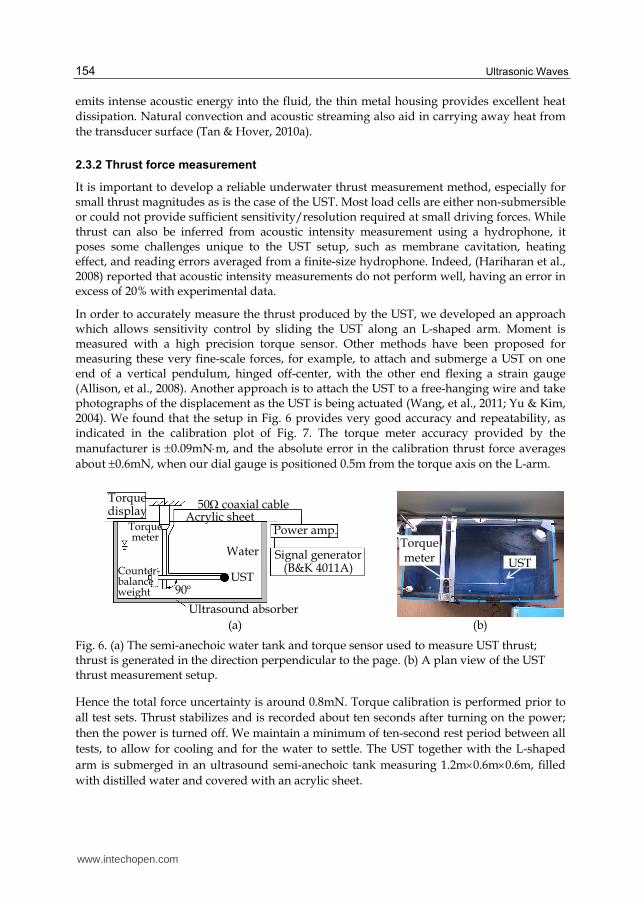
In order to accurately measure the thrust produced by the UST, we developed an approach which allows sensitivity control by sliding the UST along an L-shaped arm. Moment is measured with a high precision torque sensor. Other methods have been proposed for measuring these very fine-scale forces, for example, to attach and submerge a UST on one end of a vertical pendulum, hinged off-center, with the other end flexing a strain gauge (Allison, et al., 2008). Another approach is to attach the UST to a free-hanging wire and take photographs of the displacement as the UST is being actuated (Wang, et al., 2011; Yu & Kim, 2004). We found that the setup in Fig. 6 provides very good accuracy and repeatability, as indicated in the calibration plot of Fig. 7. The torque meter accuracy provided by the

manufacturer is 0.09mNm, and the absolute error in the calibration thrust force averages

about 0.6mN, when our dial gauge is positioned 0.5m from the torque axis on the L-arm.

(a) (b)

Fig. 6. (a) The semi-anechoic water tank and torque sensor used to measure UST thrust; thrust is generated in the direction perpendicular to the page. (b) A plan view of the UST thrust measurement setup.

Hence the total force uncertainty is around 0.8mN. Torque calibration is performed prior to

all test sets. Thrust stabilizes and is recorded about ten seconds after turning on the power;

then the power is turned off. We maintain a minimum of ten-second rest period between all

tests, to allow for cooling and for the water to settle. The UST together with the L-shaped

arm is submerged in an ultrasound semi-anechoic tank measuring 1.2m0.6m0.6m, filled

with distilled water and covered with an acrylic sheet.

Torque meter UST

Torque display

Torque meter

Acrylic sheet50 coaxial cable

Power amp.

Signal generator(B&K 4011A)

Water

USTCounter-balance weight

Ultrasound absorber

90

www.intechopen.com

Ultrasonic Thruster

155

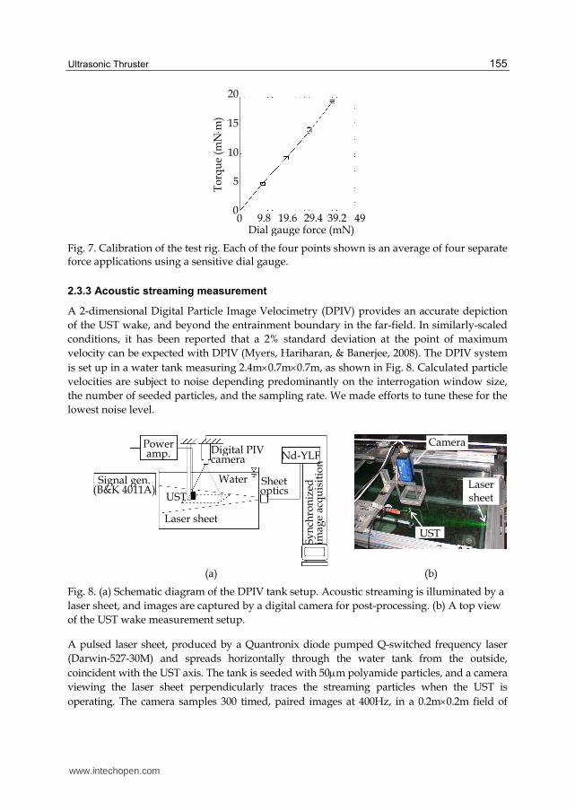
Fig. 7. Calibration of the test rig. Each of the four points shown is an average of four separate force applications using a sensitive dial gauge.

2.3.3 Acoustic streaming measurement

A 2-dimensional Digital Particle Image Velocimetry (DPIV) provides an accurate depiction

of the UST wake, and beyond the entrainment boundary in the far-field. In similarly-scaled

conditions, it has been reported that a 2% standard deviation at the point of maximum

velocity can be expected with DPIV (Myers, Hariharan, & Banerjee, 2008). The DPIV system

is set up in a water tank measuring 2.4m0.7m0.7m, as shown in Fig. 8. Calculated particle

velocities are subject to noise depending predominantly on the interrogation window size,

the number of seeded particles, and the sampling rate. We made efforts to tune these for the

lowest noise level.

(a) (b)

Fig. 8. (a) Schematic diagram of the DPIV tank setup. Acoustic streaming is illuminated by a

laser sheet, and images are captured by a digital camera for post-processing. (b) A top view

of the UST wake measurement setup.

A pulsed laser sheet, produced by a Quantronix diode pumped Q-switched frequency laser

(Darwin-527-30M) and spreads horizontally through the water tank from the outside,

coincident with the UST axis. The tank is seeded with 50m polyamide particles, and a camera

viewing the laser sheet perpendicularly traces the streaming particles when the UST is

operating. The camera samples 300 timed, paired images at 400Hz, in a 0.2m0.2m field of

20

15

10

5

00 9.8 19.6 29.4 39.2 49

Dial gauge force (mN)T

orq

ue

(mNm)

Camera

Laser sheet

UST

Water

Laser sheet

UST

Signal gen.(B&K 4011A)

Power amp. Nd-YLF

Sheet optics

Sy

nch

ron

ized

im

age

acq

uis

itio

n

Digital PIV camera

www.intechopen.com

Ultrasonic Waves

156

view. Post-processing is carried out using DaVis 7.1 software. The UST transducer is

positioned at 1.2m from the sheet optics, 0.4m from each adjacent tank wall, and 0.3m below

the water surface. The time taken for the stream to become established has been reported

variously at about 0.5s (Loh & Lee, 2004) and 20s (Kamakura, Sudo, Matsuda, & Kumamoto,

1996). We allow at least one minute of flow before the camera starts recording. Specific kinetic

energy of the flow up to the focal distance xf is shown in the next section, which averages 150

measurements; recording the frames takes less than one second. Then the power is turned off,

and the tank water is allowed to settle for at least one minute. This schedule is not the same for

thrust measurements, as the transducer is powered and cooled for a considerably longer time

during DPIV tests. A more detailed analysis of the transducer heating is presented in Section 3.

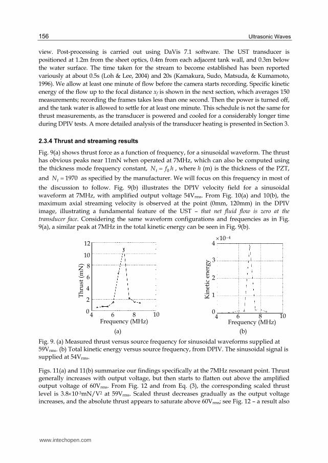
2.3.4 Thrust and streaming results

Fig. 9(a) shows thrust force as a function of frequency, for a sinusoidal waveform. The thrust

has obvious peaks near 11mN when operated at 7MHz, which can also be computed using

the thickness mode frequency constant, 0tN f h , where h (m) is the thickness of the PZT,

and 1970tN as specified by the manufacturer. We will focus on this frequency in most of

the discussion to follow. Fig. 9(b) illustrates the DPIV velocity field for a sinusoidal

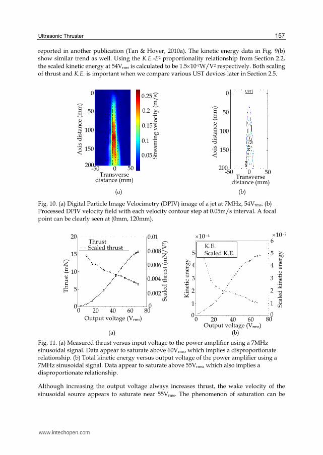
waveform at 7MHz, with amplified output voltage 54Vrms. From Fig. 10(a) and 10(b), the

maximum axial streaming velocity is observed at the point (0mm, 120mm) in the DPIV

image, illustrating a fundamental feature of the UST – that net fluid flow is zero at the

transducer face. Considering the same waveform configurations and frequencies as in Fig.

9(a), a similar peak at 7MHz in the total kinetic energy can be seen in Fig. 9(b).

(a) (b)

Fig. 9. (a) Measured thrust versus source frequency for sinusoidal waveforms supplied at 59Vrms. (b) Total kinetic energy versus source frequency, from DPIV. The sinusoidal signal is supplied at 54Vrms.

Figs. 11(a) and 11(b) summarize our findings specifically at the 7MHz resonant point. Thrust generally increases with output voltage, but then starts to flatten out above the amplified output voltage of 60Vrms. From Fig. 12 and from Eq. (3), the corresponding scaled thrust

level is 3.810-3mN/V2 at 59Vrms. Scaled thrust decreases gradually as the output voltage increases, and the absolute thrust appears to saturate above 60Vrms; see Fig. 12 – a result also

12

6

4

2

06 8 10

Frequency (MHz)

Th

rust

(m

N)

4

8

10

6 8 10Frequency (MHz)

4

3

2

1

0

4

Kin

etic

en

erg

y

10 - 4

www.intechopen.com

Ultrasonic Thruster

157

reported in another publication (Tan & Hover, 2010a). The kinetic energy data in Fig. 9(b) show similar trend as well. Using the K.E.-E2 proportionality relationship from Section 2.2,

the scaled kinetic energy at 54Vrms is calculated to be 1.510-7W/V2 respectively. Both scaling of thrust and K.E. is important when we compare various UST devices later in Section 2.5.

(a) (b)

Fig. 10. (a) Digital Particle Image Velocimetry (DPIV) image of a jet at 7MHz, 54Vrms. (b) Processed DPIV velocity field with each velocity contour step at 0.05m/s interval. A focal point can be clearly seen at (0mm, 120mm).

(a) (b)

Fig. 11. (a) Measured thrust versus input voltage to the power amplifier using a 7MHz sinusoidal signal. Data appear to saturate above 60Vrms, which implies a disproportionate relationship. (b) Total kinetic energy versus output voltage of the power amplifier using a 7MHz sinusoidal signal. Data appear to saturate above 55Vrms, which also implies a disproportionate relationship.

Although increasing the output voltage always increases thrust, the wake velocity of the

sinusoidal source appears to saturate near 55Vrms. The phenomenon of saturation can be

50

100

150

200

0

Ax

is d

ista

nce

(m

m)

0 50 Transverse

distance (mm)

-50

UST

0 50Transverse

distance (mm)

-50

Ax

is d

ista

nce

(m

m)

Str

eam

ing

vel

oci

ty (

m/

s)

0.2

0.15

0.1

0.05

0.25

50

100

150

200

0

20 40Output voltage (Vrms)

0

Sca

led

kin

etic

en

erg

y

0

3

2

1

060

1

2

3

4

5

6 10 - 7

4

5

10 - 4

80

Kin

etic

en

erg

y

K.E.Scaled K.E.

ThrustScaled thrust

0.01

0.008

0.006

0.004

0.002

0

20

15

10

5

0

Sca

led

th

rust

(m

N/

V2 )

20 400 60 80

Output voltage (Vrms)

Th

rust

(m

N)

www.intechopen.com

Ultrasonic Waves

158

explained by distortion in finite-amplitude traveling waves, according to weak shock

theory. On the other hand, the fact that thrust in this case increases with input power

despite the saturation of velocity highlights an unusual observation – that thrust production

mechanism involves the wake only indirectly, and in a manner that is distinct from other

propulsors. This fact may offer some interesting avenues for UST design, where the wake

and the thrust force could be manipulated independently. This is especially useful in a

scenario where larger thrust is desired but the wake has to be weak at the same time, for

example, to minimize stirring up particulates near the seabed.

In summary, increasing the output voltage of the power amplifier will no doubt increase the

thrust and kinetic energy production of the transducer, but at the same time, introduces an

undesirable disproportionate relationship (Tan & Hover, 2010a). This will be further

discussed in Section 3.

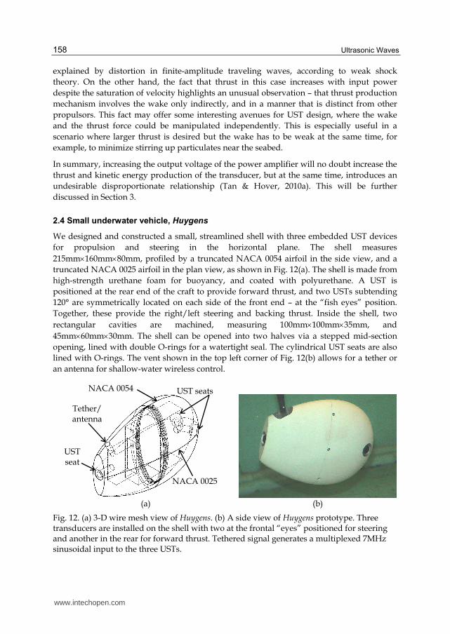
2.4 Small underwater vehicle, Huygens

We designed and constructed a small, streamlined shell with three embedded UST devices

for propulsion and steering in the horizontal plane. The shell measures

215mm160mm80mm, profiled by a truncated NACA 0054 airfoil in the side view, and a

truncated NACA 0025 airfoil in the plan view, as shown in Fig. 12(a). The shell is made from

high-strength urethane foam for buoyancy, and coated with polyurethane. A UST is

positioned at the rear end of the craft to provide forward thrust, and two USTs subtending

120° are symmetrically located on each side of the front end – at the “fish eyes” position.

Together, these provide the right/left steering and backing thrust. Inside the shell, two

rectangular cavities are machined, measuring 100mm100mm35mm, and

45mm60mm30mm. The shell can be opened into two halves via a stepped mid-section

opening, lined with double O-rings for a watertight seal. The cylindrical UST seats are also

lined with O-rings. The vent shown in the top left corner of Fig. 12(b) allows for a tether or

an antenna for shallow-water wireless control.

(a) (b)

Fig. 12. (a) 3-D wire mesh view of Huygens. (b) A side view of Huygens prototype. Three transducers are installed on the shell with two at the frontal “eyes” positioned for steering and another in the rear for forward thrust. Tethered signal generates a multiplexed 7MHz sinusoidal input to the three USTs.

UST seatsNACA 0054

NACA 0025

Tether/ antenna

UST seat

www.intechopen.com

Ultrasonic Thruster

159

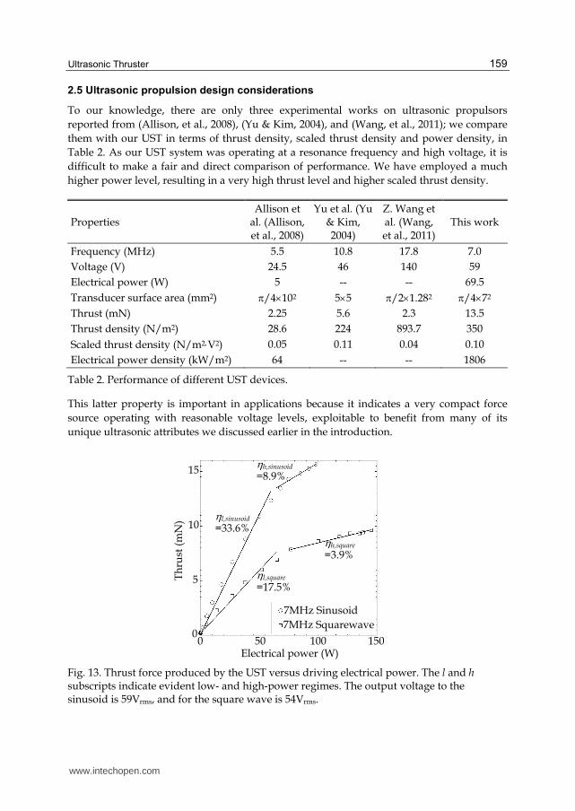
2.5 Ultrasonic propulsion design considerations

To our knowledge, there are only three experimental works on ultrasonic propulsors

reported from (Allison, et al., 2008), (Yu & Kim, 2004), and (Wang, et al., 2011); we compare

them with our UST in terms of thrust density, scaled thrust density and power density, in

Table 2. As our UST system was operating at a resonance frequency and high voltage, it is

difficult to make a fair and direct comparison of performance. We have employed a much

higher power level, resulting in a very high thrust level and higher scaled thrust density.

Properties Allison et

al. (Allison, et al., 2008)

Yu et al. (Yu & Kim, 2004)

Z. Wang et al. (Wang, et al., 2011)

This work

Frequency (MHz) 5.5 10.8 17.8 7.0

Voltage (V) 24.5 46 140 59

Electrical power (W) 5 -- -- 69.5

Transducer surface area (mm2) /4102 55 /21.282 /472

Thrust (mN) 2.25 5.6 2.3 13.5

Thrust density (N/m2) 28.6 224 893.7 350

Scaled thrust density (N/m2V2) 0.05 0.11 0.04 0.10

Electrical power density (kW/m2) 64 -- -- 1806

Table 2. Performance of different UST devices.

This latter property is important in applications because it indicates a very compact force

source operating with reasonable voltage levels, exploitable to benefit from many of its

unique ultrasonic attributes we discussed earlier in the introduction.

Fig. 13. Thrust force produced by the UST versus driving electrical power. The l and h subscripts indicate evident low- and high-power regimes. The output voltage to the sinusoid is 59Vrms, and for the square wave is 54Vrms.

50 100Electrical power (W)

0

5

0150

10

15

Th

rust

(m

N)

7MHz Sinusoid

7MHz Squarewave

h,sinusoid =8.9%

l,sinusoid

=33.6%

l,square

=17.5%

h,square

=3.9%

www.intechopen.com

Ultrasonic Waves

160

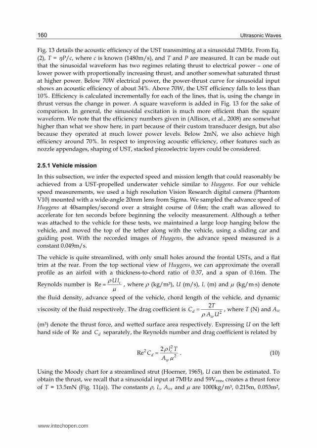
Fig. 13 details the acoustic efficiency of the UST transmitting at a sinusoidal 7MHz. From Eq.

(2), T = P/c, where c is known (1480m/s), and T and P are measured. It can be made out

that the sinusoidal waveform has two regimes relating thrust to electrical power – one of

lower power with proportionally increasing thrust, and another somewhat saturated thrust

at higher power. Below 70W electrical power, the power-thrust curve for sinusoidal input

shows an acoustic efficiency of about 34%. Above 70W, the UST efficiency falls to less than

10%. Efficiency is calculated incrementally for each of the lines, that is, using the change in

thrust versus the change in power. A square waveform is added in Fig. 13 for the sake of

comparison. In general, the sinusoidal excitation is much more efficient than the square

waveform. We note that the efficiency numbers given in (Allison, et al., 2008) are somewhat

higher than what we show here, in part because of their custom transducer design, but also

because they operated at much lower power levels. Below 2mN, we also achieve high

efficiency around 70%. In respect to improving acoustic efficiency, other features such as

nozzle appendages, shaping of UST, stacked piezoelectric layers could be considered.

2.5.1 Vehicle mission

In this subsection, we infer the expected speed and mission length that could reasonably be

achieved from a UST-propelled underwater vehicle similar to Huygens. For our vehicle

speed measurements, we used a high resolution Vision Research digital camera (Phantom

V10) mounted with a wide-angle 20mm lens from Sigma. We sampled the advance speed of

Huygens at 40samples/second over a straight course of 0.6m; the craft was allowed to

accelerate for ten seconds before beginning the velocity measurement. Although a tether

was attached to the vehicle for these tests, we maintained a large loop hanging below the

vehicle, and moved the top of the tether along with the vehicle, using a sliding car and

guiding post. With the recorded images of Huygens, the advance speed measured is a

constant 0.049m/s.

The vehicle is quite streamlined, with only small holes around the frontal USTs, and a flat

trim at the rear. From the top sectional view of Huygens, we can approximate the overall

profile as an airfoil with a thickness-to-chord ratio of 0.37, and a span of 0.16m. The

Reynolds number is Re cU l , where (kg/m3), U (m/s), lc (m) and (kg/ms) denote

the fluid density, advance speed of the vehicle, chord length of the vehicle, and dynamic

viscosity of the fluid respectively. The drag coefficient is 2

2d

w

TC

A U , where T (N) and Aw

(m3) denote the thrust force, and wetted surface area respectively. Expressing U on the left

hand side of Re and dC separately, the Reynolds number and drag coefficient is related by

2

22

2Re c

dw

l TC

A

. (10)

Using the Moody chart for a streamlined strut (Hoerner, 1965), U can then be estimated. To

obtain the thrust, we recall that a sinusoidal input at 7MHz and 59Vrms, creates a thrust force

of T = 13.5mN (Fig. 11(a)). The constants , lc, Aw, and are 1000kg/m3, 0.215m, 0.053m2,

www.intechopen.com

Ultrasonic Thruster

161

and 1.00210-3kg/ms respectively. The parameter 2Re dC , solved using Eq. (10), is 23.4106,

and for Huygens, a unique point can be identified on the RedC Moody diagram; Re =

1.17104 and 0.17dC . It is thus estimated that Huygens will advance at a velocity of

0.054m/s – very close to the observed value.

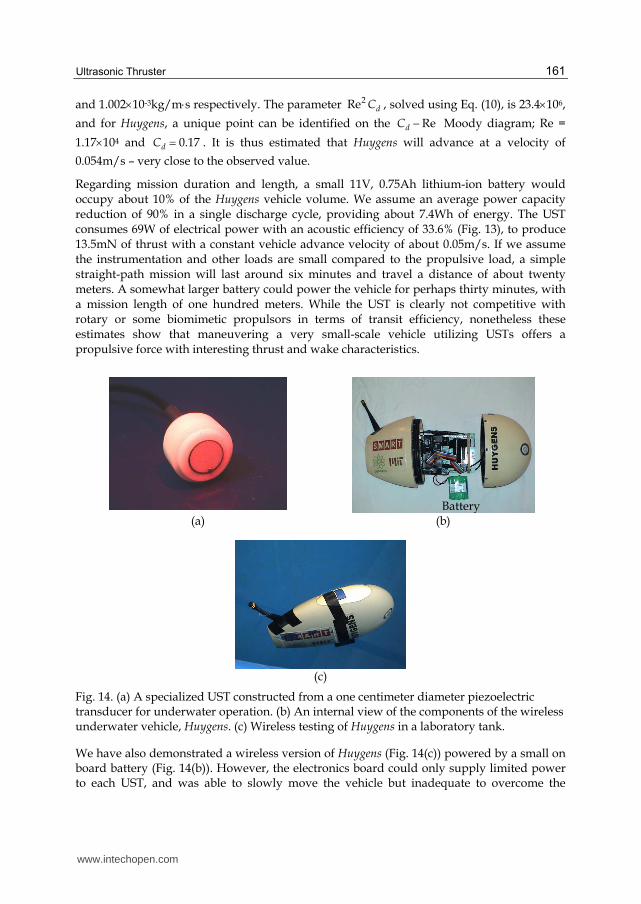
Regarding mission duration and length, a small 11V, 0.75Ah lithium-ion battery would occupy about 10% of the Huygens vehicle volume. We assume an average power capacity reduction of 90% in a single discharge cycle, providing about 7.4Wh of energy. The UST consumes 69W of electrical power with an acoustic efficiency of 33.6% (Fig. 13), to produce 13.5mN of thrust with a constant vehicle advance velocity of about 0.05m/s. If we assume the instrumentation and other loads are small compared to the propulsive load, a simple straight-path mission will last around six minutes and travel a distance of about twenty meters. A somewhat larger battery could power the vehicle for perhaps thirty minutes, with a mission length of one hundred meters. While the UST is clearly not competitive with rotary or some biomimetic propulsors in terms of transit efficiency, nonetheless these estimates show that maneuvering a very small-scale vehicle utilizing USTs offers a propulsive force with interesting thrust and wake characteristics.

(a) (b)

(c)

Fig. 14. (a) A specialized UST constructed from a one centimeter diameter piezoelectric transducer for underwater operation. (b) An internal view of the components of the wireless underwater vehicle, Huygens. (c) Wireless testing of Huygens in a laboratory tank.

We have also demonstrated a wireless version of Huygens (Fig. 14(c)) powered by a small on board battery (Fig. 14(b)). However, the electronics board could only supply limited power to each UST, and was able to slowly move the vehicle but inadequate to overcome the

Battery

www.intechopen.com

Ultrasonic Waves

162

vehicle drag very well. One solution could be to improve the UST power output through a small size ultrasound amplifier such as reported in (Lewis & Olbricht, 2008). We continue to make improvements to optimize the output thrust density with considerations to on board space budget, using specially constructed underwater UST (Fig. 14(a)), and higher energy density batteries as well.

3. Thermal dissipation of UST

As we observed in our previous work (Tan & Hover, 2009, 2010b), a disproportionate loss in thrust exist under elevated voltage applied across the transducer. As in all piezoelectric transducers, most of the electrical energy is converted into acoustical energy with some lost as superfluous heat through the transducer. In the presence of a large potential voltage, heat dissipation increases significantly, and dependent variables include the dielectric dissipation factor, transducer capacitance, and the presence of heat retardant materials next to the transducer. In instances of high power, localized heating at the soldered points may result in a failure or other undesirable outcome (Zhou & Rogers, 1995).

While temperature studies on PZT have been adequately described and investigated in the literature (Duck, Starritt, ter Haar, & Lunt, 1989; Sherrit et al., 2001), we are not aware of any work that makes a direct connection between transducer temperature rise and the propulsive thrust generated. As the UST is an underwater propulsor, knowledge of the conditions leading it to become a thermal source is important in many applications. In the following, we experimentally quantify the thermal distribution on the surface of the transducer under ultrasonic thrusting conditions, and introduce a dimensionless parameter to relate the thermal loss. In certain strategic applications, knowledge of this heat signature could aid in critical UST and system propulsion designs.

3.1 Heat transfer equations

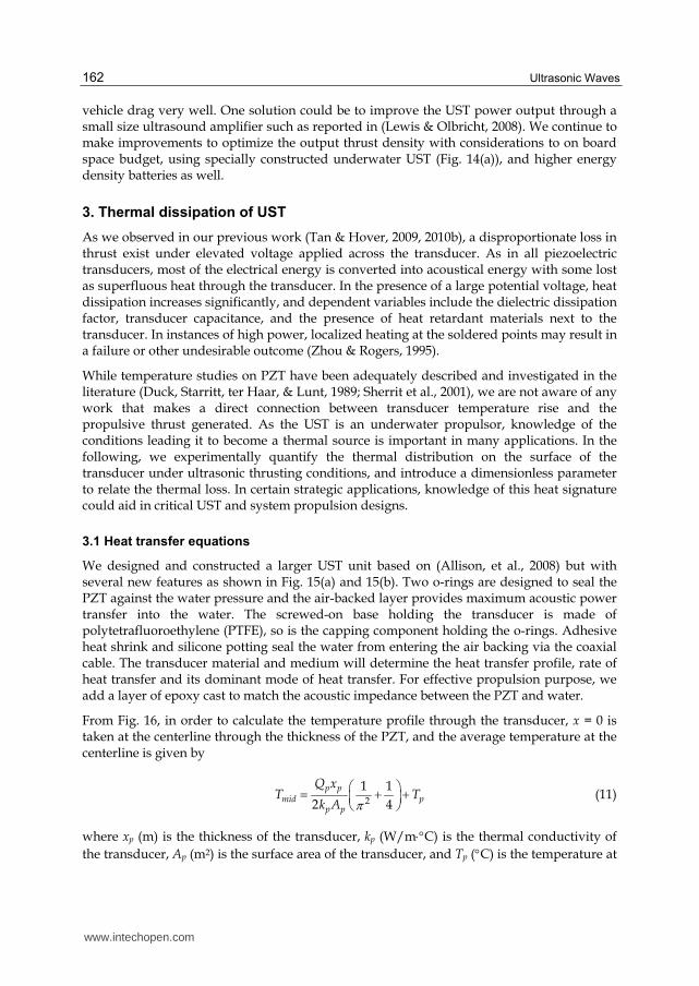
We designed and constructed a larger UST unit based on (Allison, et al., 2008) but with several new features as shown in Fig. 15(a) and 15(b). Two o-rings are designed to seal the PZT against the water pressure and the air-backed layer provides maximum acoustic power transfer into the water. The screwed-on base holding the transducer is made of polytetrafluoroethylene (PTFE), so is the capping component holding the o-rings. Adhesive heat shrink and silicone potting seal the water from entering the air backing via the coaxial cable. The transducer material and medium will determine the heat transfer profile, rate of heat transfer and its dominant mode of heat transfer. For effective propulsion purpose, we add a layer of epoxy cast to match the acoustic impedance between the PZT and water.

From Fig. 16, in order to calculate the temperature profile through the transducer, x = 0 is taken at the centerline through the thickness of the PZT, and the average temperature at the centerline is given by

2

1 1

2 4

p pmid p

p p

Q xT T

k A (11)

where xp (m) is the thickness of the transducer, kp (W/mC) is the thermal conductivity of

the transducer, Ap (m2) is the surface area of the transducer, and Tp (C) is the temperature at

www.intechopen.com

Ultrasonic Thruster

163

the interface between the transducer and epoxy layer (Sherrit, et al., 2001). Qp (W) is the

average heat transfer rate of the piezoelectric material, which is also the average power

dissipation, given by

22 tanp rmsQ f C E (12)

where f (Hz) is the resonance frequency, C (F) is the capacitance of the transducer, tan (%)

is the dielectric dissipation factor, and Erms (Vrms) is the root-mean-square of the applied

voltage. It is important to understand that under high power and temperature conditions,

the transducer’s dielectric dissipation factor will change with the voltage applied,

temperature and fluidic load. Consequently, the capacitance and dielectricity also vary

nonlinearly as the voltage and temperature increase, incurring significant errors if these are

not carefully characterized under elevated settings. The temperature profile of the

piezoelectric material takes on a parabolic distribution, peaking at Tmid (C), and either

surface of the transducer has the same temperature, Tp; see Fig. 16. In addition, as we verify

in Section 3.4 for the Biot number, we consider convection to be more important than the

internal conduction which exhibits a nearly uniform temperature gradient within the

homogenous solid body (PZT).

(a) (b)

Fig. 15. (a) Sectioned view of the modular UST. A female Teflon cap is screwed onto the base holder which holds the transducer. O-rings provide the water-tight seals, and silicone potting provides flexibility and waterproofing to the coaxial cable connection. (b) An exploded view of the components of the modular UST.

The 1-dimensional Fourier’s law is used to describe the thermal conduction of heat through

the layer of epoxy cast on the UST water-side surface, and is governed by the heat flux, q

(W/m2), and the heat transfer rate (W) is given by

p e

e e e ee

T TQ qA k A

x

(13)

where ke (W/mC) is the thermal conductivity, Te (C) is the surface temperature of the

epoxy cast facing the water, and xe (m) is the thickness of the epoxy cast. q is positive if heat

flows along the positive x-direction, and vice versa.

Silicone potting

Silicone potting

Adhesive heat shrink Coaxial cable

Matching layer

Piezo

Air

Seal

Seal

www.intechopen.com

Ultrasonic Waves

164

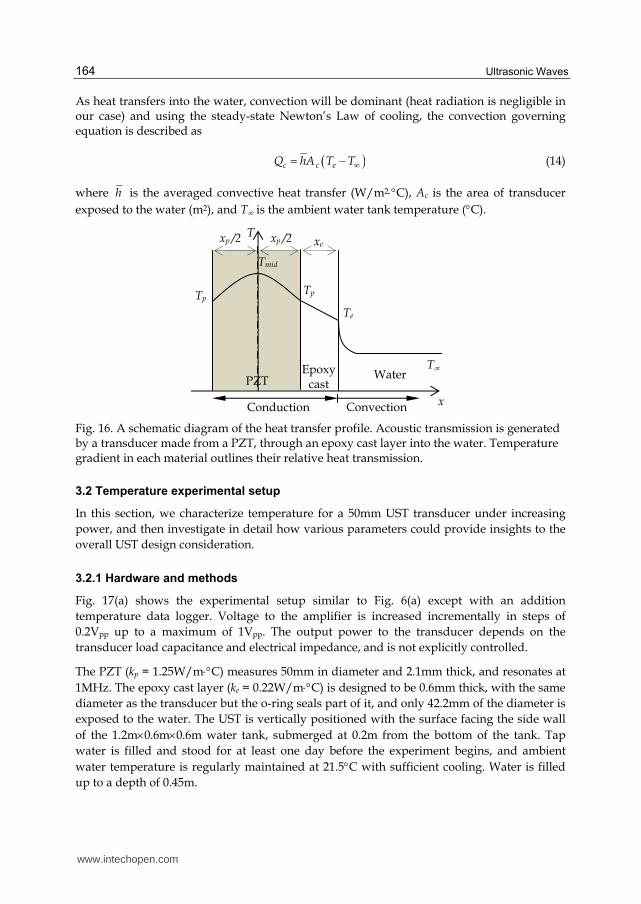
As heat transfers into the water, convection will be dominant (heat radiation is negligible in our case) and using the steady-state Newton’s Law of cooling, the convection governing equation is described as

c c eQ hA T T (14)

where h is the averaged convective heat transfer (W/m2C), Ac is the area of transducer

exposed to the water (m2), and T is the ambient water tank temperature (C).

Fig. 16. A schematic diagram of the heat transfer profile. Acoustic transmission is generated by a transducer made from a PZT, through an epoxy cast layer into the water. Temperature gradient in each material outlines their relative heat transmission.

3.2 Temperature experimental setup

In this section, we characterize temperature for a 50mm UST transducer under increasing

power, and then investigate in detail how various parameters could provide insights to the

overall UST design consideration.

3.2.1 Hardware and methods

Fig. 17(a) shows the experimental setup similar to Fig. 6(a) except with an addition

temperature data logger. Voltage to the amplifier is increased incrementally in steps of

0.2Vpp up to a maximum of 1Vpp. The output power to the transducer depends on the

transducer load capacitance and electrical impedance, and is not explicitly controlled.

The PZT (kp = 1.25W/mC) measures 50mm in diameter and 2.1mm thick, and resonates at

1MHz. The epoxy cast layer (ke = 0.22W/mC) is designed to be 0.6mm thick, with the same

diameter as the transducer but the o-ring seals part of it, and only 42.2mm of the diameter is

exposed to the water. The UST is vertically positioned with the surface facing the side wall

of the 1.2m0.6m0.6m water tank, submerged at 0.2m from the bottom of the tank. Tap

water is filled and stood for at least one day before the experiment begins, and ambient

water temperature is regularly maintained at 21.5C with sufficient cooling. Water is filled

up to a depth of 0.45m.

Tmid

PZTEpoxy

castWater

x

T

Conduction Convection

Tp Tp

Te

T

xexp /2xp /2

www.intechopen.com

Ultrasonic Thruster

165

(a) (b)

Fig. 17. (a) The experimental setup used to measure the UST temperature and thrust at the same time. Thrust is generated in the normal direction and out of the page. (b) A top view of the UST temperature measurement setup.

Similar torque calibration is performed prior to each set of test as discussed in Section 2.3.2.

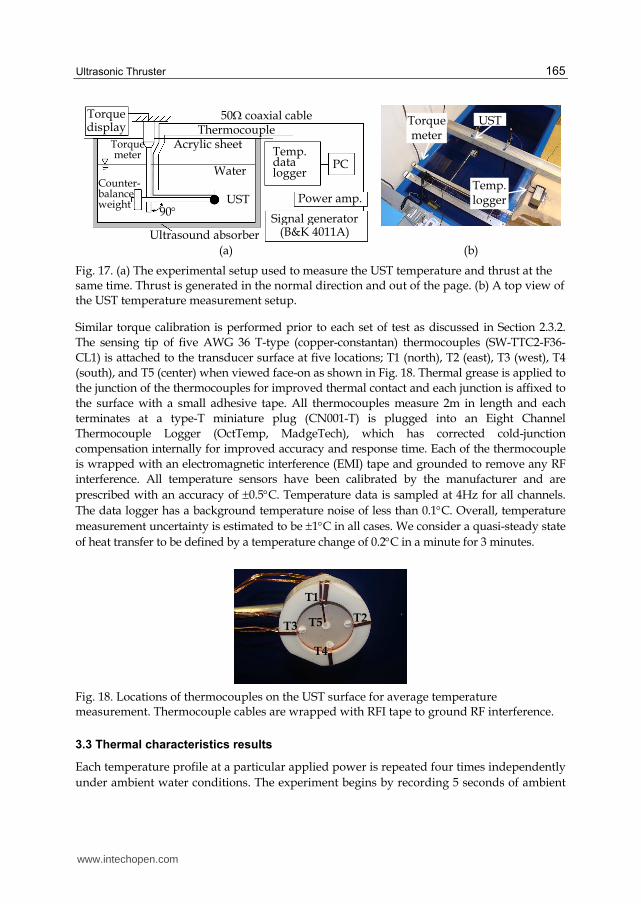
The sensing tip of five AWG 36 T-type (copper-constantan) thermocouples (SW-TTC2-F36-

CL1) is attached to the transducer surface at five locations; T1 (north), T2 (east), T3 (west), T4

(south), and T5 (center) when viewed face-on as shown in Fig. 18. Thermal grease is applied to

the junction of the thermocouples for improved thermal contact and each junction is affixed to

the surface with a small adhesive tape. All thermocouples measure 2m in length and each

terminates at a type-T miniature plug (CN001-T) is plugged into an Eight Channel

Thermocouple Logger (OctTemp, MadgeTech), which has corrected cold-junction

compensation internally for improved accuracy and response time. Each of the thermocouple

is wrapped with an electromagnetic interference (EMI) tape and grounded to remove any RF

interference. All temperature sensors have been calibrated by the manufacturer and are

prescribed with an accuracy of 0.5C. Temperature data is sampled at 4Hz for all channels.

The data logger has a background temperature noise of less than 0.1C. Overall, temperature

measurement uncertainty is estimated to be 1C in all cases. We consider a quasi-steady state

of heat transfer to be defined by a temperature change of 0.2C in a minute for 3 minutes.

Fig. 18. Locations of thermocouples on the UST surface for average temperature measurement. Thermocouple cables are wrapped with RFI tape to ground RF interference.

3.3 Thermal characteristics results

Each temperature profile at a particular applied power is repeated four times independently

under ambient water conditions. The experiment begins by recording 5 seconds of ambient

T1

T2T3

T4

T5

Torque meter

UST

Temp. logger

Torque display

Torque meter

Acrylic sheet

50 coaxial cable

PC

Signal generator(B&K 4011A)

Water

UST

Counter-balance weight

Ultrasound absorber

90

Temp. data logger

Thermocouple

Power amp.

www.intechopen.com

Ultrasonic Waves

166

water temperature, after which the power amplifier is switched on for about 9mins. During

this time, the transducer is observed to increase its temperature steadily and then stabilizes.

9mins into the actuation, all thermocouple achieve a quasi-steady state and the power

amplifier is switched off. Cooling proceeds for another 10mins and the tank is allowed to

settle. Ambient temperature of the water tank is monitored separately at the start and end of

the experiment, and further cooling is allowed if the ambient water temperature increased

significantly.

Generally, increasing the input voltage (in steps of 0.2Vpp to 1.0Vpp) to the amplifier

increases the temperature recorded on the transducer surface. Table 3 summarizes the input

voltage to the amplifier, output voltage and output power of the amplifier, the

corresponding thrust, and the mean transducer surface temperature. Four sets of data are

each tabulated for the output voltage, output power, and thrust, to demonstrate the

consistency of the system.

Using the output power and thrust columns of Table 3, a plot of thrust versus power is

shown in Fig. 19. From Eq. (2), the acoustic efficiency of the UST can be worked out, which

essentially is the gradient at each cluster of points multiply by the speed of sound in the

water, c. Generally at lower power, the efficiency is higher, however, effective thrust is also

lower, which may not be practically useful. As the power increases, efficiency declines

rapidly and Fig. 19 illustrates the trend. In Fig. 19, it can be seen that generated thrust starts

to decline at higher electrical power level. However, as we discuss below, the acoustic

efficiency is observed to vary approximately in a first-order fashion as P increases.

Ultrasonic thrust appears to begin to saturate near 16mN.

Input

voltage

(Vpp)

Output

voltage

(Vrms)

Output power (W) Thrust (mN)

Mean

surface

temp. (C)

0.2 13, 13, 12, 13 3.2, 3.2, 2.9, 3.2 4.59, 4.44, 4.59, 4.52 22.9

0.4 30, 29, 28, 29 18.0, 16.8, 15.6, 16.8 7.08, 7.01, 6.93, 6.86 26.7

0.6 48, 47, 47, 48 45.6, 43.6, 43.6, 45.6 10.85, 10.70, 10.70, 10.78 30.6

0.8 67, 66, 66, 67 90.4, 87.2, 87.2, 90.4 14.85, 14.77, 14.62, 14.85 35.0

1.0 86, 84, 86, 86 147.8, 141.8, 147.8,

147.8

16.43, 16.43, 16.5, 16.35,

16.5 39.2

Table 3. Table of output power from the amplifier and the corresponding thrust generated. Four sets of data from each stepped input voltage are recorded. Ambient tank temperature

is maintained at 21.5C.

3.3.1 Thermal losses at high voltage

To calculate the averaged convective heat transfer, we use the lumped-capacity solution for

a heated body transferring heat into the water by free convection. The solution can be solved

for T (t = 0) to give (Lienhard IV & Lienhard V, 2002)

t

eT T T e T (15)

www.intechopen.com

Ultrasonic Thruster

167

where T (C) is the time-variant temperature of the epoxy with respect to time t (s), Te (C) is

the averaged temperature of the epoxy surface determined as [22.9, 26.7, 30.6, 35.0, 39.2]C

from the stepped input voltage, and T (C) is the ambient tank temperature at

21.5C. e e e

e

c V

h A

is the time constant of the cooling process, where = 1200 kg/m3 is the

density of the epoxy, ce = 1110 J/kgC is the specific heat capacity of epoxy, Ve = 8.410-7m3

is the volume of the epoxy through which sound transmits, h (W/m2C) is the average

convective heat transfer coefficient determined as [25, 24, 22, 18, 14]W/m2C from the

stepped input voltage, and Ae = 5.610-3m2 is the cross-sectional area of the epoxy through which sound transmits (note Ae = Ap).

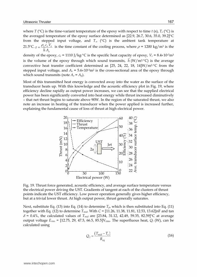
Most of this transmitted heat energy is convected away into the water as the surface of the transducer heats up. With this knowledge and the acoustic efficiency plot in Fig. 19, where efficiency decline rapidly as output power increases, we can see that the supplied electrical power has been significantly converted into heat energy while thrust increased diminutively – that net thrust begins to saturate above 90W. In the region of the saturated thrust, we also note an increase in heating of the transducer when the power applied is increased further, explaining the fundamental cause of loss of thrust at high electrical power.

Fig. 19. Thrust force generated, acoustic efficiency, and average surface temperature versus the electrical power driving the UST. Gradients of tangent at each of the clusters of thrust points indicate the UST efficiency. Low power operation generally gives higher efficiency, but at a trivial lower thrust. At high output power, thrust generally saturates.

Next, substitute Eq. (13) into Eq. (14) to determine Tp, which is then substituted into Eq. (11) together with Eq. (12) to determine Tmid. With C = [11.26, 11.38, 11.81, 12.53, 13.62]nF and tan ≈ 0.4%, the calculated values of Tmid are [23.84, 31.12, 42.49, 59.35, 82.59]C at average output voltage Erms = [12.75, 29, 47.5, 66.5, 85.5]Vrms. The superfluous heat, Ql (W), can be calculated using

mid el

eq

T TQ

R

(16)

EfficiencyThrustTemperature

20

18

16

14

12

10

8

6

4

2

00 50 100 150

Electrical power (W)

10

20

30

40

50

60

22

24

26

28

30

32

34

36

38

40

Th

rust

(m

N)

Av

e. t

ran

sdu

cer

surf

ace

tem

p. (C)

Eff

icie

ncy

(%

)

0

2a

JetUST

www.intechopen.com

Ultrasonic Waves

168

where the equivalent thermal resistance, 2

1 14

4

pe

eqp p e e

xx

Rk A k A , for the transducer

distance from x = 0 to the epoxy surface. We plot this heat loss against the amplifier output

voltage, Erms, in Fig. 20. Introducing a dimensionless parameter, lQP

, which is the ratio of

the heat loss energy Eq. (16) to the electrical power supplied Eq. (4), as

2

Rel mid e

eq rms

Q T T

P R E

. (17)

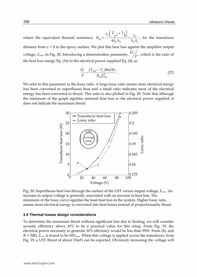
We refer to this parameter as the lossy ratio. A large lossy ratio means more electrical energy

has been converted to superfluous heat and a small ratio indicates most of the electrical

energy has been converted to thrust. This ratio is also plotted in Fig. 20. Note that although

the minimum of the graph signifies minimal heat loss to the electrical power supplied, it

does not indicate the maximum thrust.

Fig. 20. Superfluous heat loss through the surface of the UST versus output voltage, Erms. An increase in output voltage is generally associated with an increase in heat loss. The minimum of the lossy curve signifies the least heat loss in the system. Higher lossy ratio means more electrical energy is converted into heat losses instead of proportionately thrust.

3.4 Thermal losses design considerations

To determine the maximum thrust without significant loss due to heating, we will consider acoustic efficiency above 10% to be a practical value for this setup. From Fig. 19, the electrical power necessary to generate 10% efficiency would be less than 95W. From (4), and

= 50, Erms is found to be 69Vrms. When this voltage is applied across the transducer, from Fig. 19, a UST thrust of about 15mN can be expected. Obviously increasing the voltage will

UST

Average temp.

0.205

0.2

0.195

0.19

0.185

0.18

0.1750 20 40 60 80 100

Transducer heat lossLossy ratio

0

5

10

15

20

25

30

Voltage (V)

Lo

ssy

rat

io

Tra

nsd

uce

r h

eat

loss

(W

)

www.intechopen.com

Ultrasonic Thruster

169

increase the thrust but not appreciably; instead most added energy will be converted to heat losses, which becomes undesirable in the UST design scheme.

Finally, we verify that Tmid is not higher than the Curie temperature of the transducer,

specified by the manufacturer at 320C, to maintain its poled lattice integrity. We also validate the Biot number (Bi), which must be Bi « 1 to justify the temperature within the

transducer to be relatively even. From the above parameters, Bi e

e

hxk

= [0.0682, 0.0655,

0.0600, 0.0491, 0.0382]. More importantly, this condition must also be satisfied for lump-capacity solution in Eq. (15) to be accurate.

4. Conclusion

The ultrasonic thruster technology could bring about interesting and novel attributes to robotic propulsion devices and systems. These include low cost and high robustness when applied at the centimeter scale or smaller. The robustness is due to the fact that the UST effectively has no moving parts, and will not biofoul – these are properties unavailable in the rotary and biomimetic propulsors in use today. Our experiments indicated that frequency, and voltage level can both strongly influence the behavior of the UST, in terms of wake, thrust, and efficiency. We have successfully implemented three sub-centimeter UST devices into a small robot, and made calculations showing short missions can be developed with such craft, despite its inherently low propulsive efficiency.

We have also studied the heating of ultrasonic transducers under conditions of thrust production. In view of practical application of the ultrasonic transducer in the medical field, it has been reported that clinical ultrasonic probes generate considerable heat when driven at off-resonance frequencies (Duck, et al., 1989). Most medical ultrasonic devices have a safety regulation on the level of power that the transducer can produce; for example, the IEC

Standard 60606-2-37 limits the surface temperature of ultrasonic transducer to 43C. In

extreme cases, ultrasonic probes could reach a steady-state temperature of 80C in ambient air at 25°C; obviously this is not suitable for human contact in practice. While the UST is not subject to complying with this standard, a UST device is still limited by extreme heating which may cause physical damage, and also because at high temperature conditions it suffers a saturation in thrust. It may be possible to minimize or harness heat for recycling in the UST system architecture, or even recoup a part of it through specialized nozzle appendages so as to enhance efficiency. For example, the backing layer of the transducer can be ventilated or cooled to remove heat. (Deardorff & Diederich, 2000) demonstrated using a water-cooling system and reported not only it does not reduce the acoustic intensity or beam distribution, but also allows more than 45W additional power supplied to the transducer. Indeed, its thrust assistive quality remains to be investigated.

Clearly UST technology would benefit from further developmental work on application-specific areas. The UST could, for example, complement an existing propulsor system to fine tune maneuvering, or to strategically control or manipulate a flow-field for other purposes. Propulsive efficiency could conceivably be enhanced by developing a waveguide external to the transducer. The use of DPIV for characterizing UST properties is considerably richer than velocity measurement using hot wire method alone, and could also aid new transducer designs traceable to the wake field. New applications, designed to exploit the above UST’s

www.intechopen.com

Ultrasonic Waves

170

unique attributes, will certainly find this technology a valuable solution. With these insights, the UST could uncover its potential as an enabler for very small crafts, and might find uses in other completely separate applications.

5. Acknowledgment

This research was supported by the Singapore National Research Foundation (NRF) through the Singapore-MIT Alliance for Research and Technology (SMART) Centre, Centre for Environmental Sensing and Modeling (CENSAM). The authors are also grateful to M. Triantafyllou and B. Simpson for access to a DPIV system.

6. References

Allison, E. M., Springer, G. S., & Van Dam, J. (2008). Ultrasonic propulsion. Journal of

Propulsion and Power, 24(Compendex), 547-553.

Blackstock, D. T. (2000). Fundamentals of physical acoustics: New York : Wiley.

Carlton, J. (2007). Marine propellers and propulsion: Oxford : Butterworth-Heinemann.

Deardorff, D. L., & Diederich, C. J. (2000). Ultrasound applicators with internal water-

cooling for high-powered interstitial thermal therapy. IEEE Transactions on

Biomedical Engineering, 47(Compendex), 1356-1365.

Doty, K. L., Arroyo, A. A., Crane, C., Jantz, S., Novick, D., Pitzer, R., et al. (1998). An

autonomous micro-submarine swarm and miniature submarine delivery system concept.

Paper presented at the Florida Conference on Recent Advances in Robotics,

Florida.

Duck, F. A., Starritt, H. C., ter Haar, G. R., & Lunt, M. J. (1989). Surface heating of diagnostic

ultrasound transducers. British Journal of Radiology, 62(Copyright 1990, IEE), 1005-

1013.

Egeskov, P., Bech, M., Bowley, R., & Aage, C. (1995). Pipeline inspection using an autonomous

underwater vehicle. Paper presented at the Proceedings of the 14th International

Conference on Offshore Mechanics and Arctic Engineering. Part 5 (of 5), June 18,

1995 - June 22, 1995, Copenhagen, Den.

Hariharan, P., Myers, M. R., Robinson, R. A., Maruvada, S. H., Sliwa, J., & Banerjee, R. K.

(2008). Characterization of high intensity focused ultrasound transducers using

acoustic streaming. Journal of the Acoustical Society of America, 123(Compendex),

1706-1719.

Hoerner, S. F. (1965). Fluid-dynamic drag: practical information on aerodynamic drag and

hydrodynamic resistance: Midland Park, N. J.

Kamakura, T., Sudo, T., Matsuda, K., & Kumamoto, Y. (1996). Time evolution of acoustic

streaming from a planar ultrasound source. Journal of the Acoustical Society of

America, 100(Compendex), 132-132.

Lewis, G. K., & Olbricht, W. L. (2008). Development of a portable therapeutic and high

intensity ultrasound system for military, medical, and research use. Review of

Scientific Instruments, 79(Compendex).

Lienhard IV, J. H., & Lienhard V, J. H. (2002). A heat transfer textbook Cambridge, Mass. :

Phlogiston Press.

www.intechopen.com

Ultrasonic Thruster

171

Lighthill, J. (1978). Acoustic streaming. Journal of Sound and Vibration, 61(Copyright 1979,

IEE), 391-418.

Loh, B.-G., & Lee, D.-R. (2004). Heat transfer characteristics of acoustic streaming by

longitudinal ultrasonic vibration. Journal of Thermophysics and Heat Transfer,

18(Compendex), 94-99.

Myers, M. R., Hariharan, P., & Banerjee, R. K. (2008). Direct methods for characterizing high-

intensity focused ultrasound transducers using acoustic streaming. Journal of the

Acoustical Society of America, 124(Compendex), 1790-1802.

Nobunaga, S. (2004). European Patent Office: H. Electronic.

Panchal, C. B., Takahashi, P. K., & Avery, W. (1995). Biofouling control using ultrasonic and

ultraviolet treatments (pp. 13): Department of Energy, Office of Scientific and

Technical Information (DOE-OSTI).

Rudenko, O. V., & Soluian, S. I. (1977). Theoretical foundations of nonlinear acoustics. 274.

Sfakiotakis, M., Lane, D. M., & Davies, J. B. C. (1999). Review of fish swimming modes for

aquatic locomotion. IEEE Journal of Oceanic Engineering, 24(Compendex), 237-252.

Sherrit, S., Bao, X., Sigel, D. A., Gradziel, M. J., Askins, S. A., Dolgin, B. P., et al. (2001).

Characterization of transducers and resonators under high drive levels. Paper presented

at the 2001 IEEE Ultrasonics Symposium. Proceedings. An International

Symposium, 7-10 Oct. 2001, Piscataway, NJ, USA.

Tan, A. C. H., & Hover, F. S. (2009). Correlating the ultrasonic thrust force with acoustic

streaming velocity. Paper presented at the 2009 IEEE International Ultrasonics

Symposium, 20-23 Sept. 2009, Piscataway, NJ, USA.

Tan, A. C. H., & Hover, F. S. (2010a). On the influence of transducer heating in underwater

ultrasonic thrusters. Paper presented at the the 20th International Congress on

Acoustics Sydney, Australia.

Tan, A. C. H., & Hover, F. S. (2010b). Thrust and wake characterization in small, robust ultrasonic

thrusters. Paper presented at the 2010 OCEANS MTS/IEEE SEATTLE, 20-23 Sept.

2010, Piscataway, NJ, USA.

Tan, A. C. H., & Tanaka, N. (2006). The safety issues of intense airborne ultrasound: Parametric

array loudspeaker. Paper presented at the Proceedings of the 13th International

Congress on Sound and Vibration, Vienna, Austria.

Trimmer, W., & Jebens, R. (1989). Actuators for micro robots. Paper presented at the

Proceedings. 1989 IEEE International Conference on Robotics and Automation (Cat.

No.89CH2750-8), 14-19 May 1989, Washington, DC, USA.

Wang, Z., Zhu, J., Qiu, X., Tang, R., Yu, C., Oiler, J., et al. (2011). Directional acoustic

underwater thruster. Paper presented at the 2011 IEEE 24th International Conference

on Micro Electro Mechanical Systems (MEMS 2011), 23-27 Jan. 2011, Piscataway,

NJ, USA.

Yu, H., & Kim, E. S. (2004). Ultrasonic underwater thruster. Paper presented at the 17th IEEE

International Conference on Micro Electro Mechanical Systems (MEMS): Maastricht

MEMS 2004 Technical Digest, January 25, 2004 - January 29, 2004, Maastricht,

Netherlands.

www.intechopen.com

Ultrasonic Waves

172

Zhou, S.-W., & Rogers, C. A. (1995). Heat generation, temperature, and thermal stress of

structurally integrated piezo-actuators. Journal of Intelligent Material Systems and

Structures, 6(Compendex), 372-379.

www.intechopen.com

Ultrasonic WavesEdited by Dr Santos

ISBN 978-953-51-0201-4Hard cover, 282 pagesPublisher InTechPublished online 07, March, 2012Published in print edition March, 2012

InTech EuropeUniversity Campus STeP Ri Slavka Krautzeka 83/A 51000 Rijeka, Croatia Phone: +385 (51) 770 447 Fax: +385 (51) 686 166www.intechopen.com

InTech ChinaUnit 405, Office Block, Hotel Equatorial Shanghai No.65, Yan An Road (West), Shanghai, 200040, China

Phone: +86-21-62489820 Fax: +86-21-62489821

Ultrasonic waves are well-known for their broad range of applications. They can be employed in various fieldsof knowledge such as medicine, engineering, physics, biology, materials etc. A characteristic presented in allapplications is the simplicity of the instrumentation involved, even knowing that the methods are mostly verycomplex, sometimes requiring analytical and numerical developments. This book presents a number of state-of-the-art applications of ultrasonic waves, developed by the main researchers in their scientific fields from allaround the world. Phased array modelling, ultrasonic thrusters, positioning systems, tomography, projection,gas hydrate bearing sediments and Doppler Velocimetry are some of the topics discussed, which, togetherwith materials characterization, mining, corrosion, and gas removal by ultrasonic techniques, form an excitingset of updated knowledge. Theoretical advances on ultrasonic waves analysis are presented in every chapter,especially in those about modelling the generation and propagation of waves, and the influence of Goldberg'snumber on approximation for finite amplitude acoustic waves. Readers will find this book ta valuable source ofinformation where authors describe their works in a clear way, basing them on relevant bibliographicreferences and actual challenges of their field of study.

How to referenceIn order to correctly reference this scholarly work, feel free to copy and paste the following:

Alfred C. H. Tan and Franz S. Hover (2012). Ultrasonic Thruster, Ultrasonic Waves, Dr Santos (Ed.), ISBN:978-953-51-0201-4, InTech, Available from: http://www.intechopen.com/books/ultrasonic-waves/ultrasonic-thruster