Ultra-Low NOx Natural Gas Vehicle Evaluation ISL G NZ CWI LowNOx NG_Finalv06.pdf · Final Report Ultra-Low NO x Natural Gas Vehicle Evaluation ISL G NZ November 2016 Submitted by:

Final Report

Ultra-Low NOx Natural Gas Vehicle Evaluation

ISL G NZ

November 2016

Submitted by:

Author: Dr. Kent Johnson (PI)

PhD. Candidate Yu (Jade) Jiang

PhD. Candidate Jiacheng (Joey) Yang

College of Engineering-Center for Environmental Research and Technology

University of California

Riverside, CA 92521

(951) 781-5791

(951) 781-5790 fax

ii

Disclaimer

This report was prepared as a result of work sponsored in part by the California Energy

Commission (Commission), the South Coast Air Quality Management District (SCAQMD),

Southern California Gas Company (SoCalGas). It does not necessarily represent the views of the

Commission, SCAQMD, or SoCal Gas, their employees, or the State of California. The

Commission, SCAQMD, SoCalGas, the State of California, their employees, contractors, and

subcontractors make no warranty, express or implied, and assume no legal liability for the

information in this report; nor does any party represent that the use of this information will not

infringe upon privately owned rights. This report has not been approved or disapproved by the

Commission nor has the Commission passed upon the accuracy or adequacy of the information

in this report.

The statements and conclusions in this report are those of the author and not necessarily those of

Cummins Westport, Inc. The mention of commercial products, their source, or their use in

connection with material reported herein is not to be construed as actual or implied endorsement

of such products.

Inquiries related to this final report should be directed to Kent Johnson (951) 781 5786,

[email protected].

Acknowledgments

The work reported herein was performed for Cummins Westport, Inc., as part of SCAQMD

Contract No. 15626 with Cummins Westport, Inc. The work was partially funded by SCAQMD

and by CEC Contract 600-13-008 with SCAQMD and SoCalGas Agreement No. 5662230866

with SCAQMD.

The authors acknowledge Mr. Don Pacocha, Mr. Eddie O’Neil, Mr. Mark Villa, and Mr. Daniel

Gomez of CE-CERT for performing the tests and preparing the equipment for testing and Ms.

Rachael Hirst for her analytical support for the particulate matter laboratory measurements.

mailto:[email protected]

iii

Table of Contents

Table of Contents ......................................................................................................................... iii List of Tables ................................................................................................................................. v List of Figures ................................................................................................................................ v Abstract ......................................................................................................................................... vi Acronyms and Abbreviations .................................................................................................... vii

Executive Summary ................................................................................................................... viii 1 Background ......................................................................................................................... 11

1.1 Introduction ....................................................................................................................... 11 1.2 NOx Emissions .................................................................................................................. 11 1.3 Fuel economy .................................................................................................................... 12

1.4 Objectives ......................................................................................................................... 13

2 Approach ............................................................................................................................. 14 2.1 Test article ......................................................................................................................... 14

2.1.1 Engine ....................................................................................................................... 14

2.1.2 Test Fuel.................................................................................................................... 14 2.1.3 Vehicle inspection ..................................................................................................... 15 2.1.4 Test cycles ................................................................................................................. 15

2.1.5 Work calculation ....................................................................................................... 16 2.2 Laboratories ...................................................................................................................... 17

2.2.1 Chassis dynamometer ............................................................................................... 18 2.2.1.1 Test weight ...................................................................................................... 18 2.2.1.2 Coast down...................................................................................................... 19

2.2.2 Emissions measurements .......................................................................................... 19

2.2.2.1 Traditional method .......................................................................................... 19 2.2.2.2 NOx Method upgrades..................................................................................... 20 2.2.2.3 Calculation upgrades ....................................................................................... 21

2.2.3 Method evaluation .................................................................................................... 23

3 Results .................................................................................................................................. 27 3.1 Gaseous emissions ............................................................................................................ 27

3.1.1 NOx emissions .......................................................................................................... 27

3.1.2 Other gaseous emissions ........................................................................................... 28 3.2 PM emissions .................................................................................................................... 30 3.3 PN emissions ..................................................................................................................... 31 3.4 Ultrafines........................................................................................................................... 33

3.5 Greenhouse gases .............................................................................................................. 33 3.6 Fuel economy .................................................................................................................... 34

4 Discussion............................................................................................................................. 36 4.1 Transient emissions ........................................................................................................... 36 4.2 Cold start emissions .......................................................................................................... 38

5 Summary and Conclusions ................................................................................................ 39 References .................................................................................................................................... 40 Appendix A. Test Log ................................................................................................................ 42 Appendix B. Test Cycle Description .......................................................................................... 44

iv

Appendix C. UCR Mobile Emission Laboratory ....................................................................... 51

Appendix D. Heavy-Duty Chassis Dynamometer Laboratory ................................................... 52 Appendix E. Additional Test Data and Results ......................................................................... 55 Appendix F. Engine certification data, labels, and upgrades ..................................................... 60

Appendix G. Coastdown methods .............................................................................................. 65

v

List of Tables

Table 2-1 Summary of selected main engine specifications ......................................................... 14 Table 2-2 Fuel properties for the local NG test fuels utilized....................................................... 15 Table 2-3 NOx measurement methods traditional and upgraded .................................................. 21 Table 2-4 Cycle averaged raw, dilute, and ambient measured concentrations (ppm) statistics ... 23

Table 2-5 NOx emission average percent difference from Method 1 ........................................... 25 Table 2-6 Comparison to traditional Method 1 measurement (modal dilute NOx) ...................... 25 Table 3-1 PN Emissions from the ISL-G NZ 8.9 liter engine for various cycles ......................... 32 Table 3-1 Statistical comparison to the UDDSx2 test cycle ......................................................... 33 Table 3-2 Global warming potential for the ISLG NZ vehicle tested (g/bhp-hr) ......................... 34

List of Figures

Figure 1-1 Engine dynamometer NOx and PM certification emissions standards (source CWI) . 11 Figure 1-2 In-use emissions from a heavy duty truck tested on UCR’s chassis dyno .................. 12

Figure 1-3 NOx emissions versus fuel consumption tradeoffs during certification testing ......... 12 Figure 2-1 Published ISLG 8.9 Natural Gas engine power curve ................................................ 16 Figure 2-2 Power from the various tests with 1 stdev error bars .................................................. 17

Figure 2-3 Work from the various tests with 1 stdev error bars ................................................... 17 Figure 2-4 UCR’s heavy duty chassis eddy current transient dynamometer ................................ 18

Figure 2-5 Major Systems within UCR’s Mobile Emission Lab (MEL) ...................................... 20 Figure 2-6 Ambient fraction of dilute NOx concentration distribution......................................... 24 Figure 3-1 Measured NOx emission for the various test cycles ................................................... 28

Figure 3-2 Hydrocarbon emission factors (g/bhp-hr) ................................................................... 29

Figure 3-3 CO emission factors (g/bhp-hr) ................................................................................... 29 Figure 3-4 Ammonia emission factors (g/bhp-hr) ........................................................................ 30 Figure 3-5 Ammonia measured tail pipe concentration (ppm) ..................................................... 30

Figure 3-6 PM emission factors (mg/bhp-hr) ............................................................................... 31 Figure 3-7 Particle number emissions (# and #/mi) ...................................................................... 32 Figure 3-8 EEPS ultrafine PSD measurements for each of the test cycles ................................... 33

Figure 3-9 CO2 emission factors (g/bhp-hr) ................................................................................. 35 Figure 4-1 Real-time mass rate NOx emissions (g/sec) UDDS cycles ......................................... 36 Figure 4-2 Accumulated mass NOx emissions UDDS cycles ...................................................... 37 Figure 4-3 Real time NOx emissions (percent of total) ................................................................ 37 Figure 4-4 Real time NOx emissions large spike evaluation ........................................................ 38

Figure 4-5 Accumulated NOx emissions hot vs cold UDDS comparison .................................... 38

vi

Abstract

Heavy duty on-road vehicles represent one of the largest sources of NOx emissions and fuel

consumption in North America. Heavy duty vehicles are predominantly diesels, with the recent

interest in natural gas (NG) systems. As emissions and greenhouse gas regulations continue to

tighten new opportunities for advanced fleet specific heavy duty vehicles are becoming available

with improved fuel economy. NOx emissions have dropped 90% for heavy duty vehicles with the

recent 2010 certification limit. Additional NOx reductions of another 90% are desired for the

South Coast Air basin to meet its 2023 NOx inventory requirements.

Although the 2010 certification standards were designed to reduce NOx emissions, the in-use

NOx emissions are actually much higher than certification standards. The main reason is a result

of the poor performance of aftertreatment systems for diesel vehicles during low duty cycle

operation. Recent studies by UCR suggest 99% of the operation within 10 miles of the ports

represented by up to 1 g/bhp-hr. Thus, a real NOx success will not only be providing a solution

that is independent of duty cycle, but one that also reduces the emissions an additional 90% from

the current 2010 standard.

The ISL G NZ 8.9 liter NG engine met and exceeded the target NOx emissions of 0.02 g/bhp-hr

and maintained those emissions during a full ration of duty cycles found in the South Coast Air

Basin. The other gaseous, particulate matter, particle number and selected non regulated

emissions were similar to previous levels. It is expected NG vehicles could play a role in the

reduction of the south coast NOx inventory problem given their near zero emission factors

demonstrated.

vii

Acronyms and Abbreviations

ARB ...................................................Air Resources Board

bs ........................................................brake specific

CE-CERT ...........................................College of Engineering-Center for Environmental Research

and Technology (University of California, Riverside)

CFR ....................................................Code of Federal Regulations

CO ......................................................carbon monoxide

CO2 .....................................................carbon dioxide

CNG ...................................................compressed natural gas

CWI ....................................................Cummins Westport Inc.

FID .....................................................flame ionization detector

NH3 ....................................................ammonia

g/bhp-hr ..............................................grams per brake horsepower hour

lpm .....................................................liters per minute

MEL ...................................................mobile emission laboratory

NOx ....................................................nitrogen oxides

N2O ....................................................nitrous oxides

OEM ...................................................original equipment manufacturer

PM ......................................................particulate matter

PM2.5 ..................................................ultra-fine particulate matter less than 2.5 µm (certification

gravimetric reference method)

PN ......................................................particle number

PSD ....................................................particle size distribution

RPM ...................................................revolutions per minute

scfm ....................................................standard cubic feet per minute

THC....................................................total hydrocarbons

UCR ...................................................University of California at Riverside

FE .......................................................Fuel economy

GDE ...................................................gallons diesel equivalent

NG ......................................................natural gas

LNG ...................................................liquid natural gas

viii

Executive Summary


consumption in North America. Heavy duty vehicles are predominantly diesels, with the recent

penetration of natural gas (NG) engines in refuse collection, transit, and local delivery where

vehicles are centrally garaged and fueled. As emissions and greenhouse gas regulations continue

to tighten, new opportunities to use advanced fleet specific heavy duty vehicles with improved

fuel economy are becoming available. NOx emissions have dropped 90% for heavy duty vehicles

with the recent 2010 certification limit. Additional NOx reductions of another 90% are desired

for the South Coast Air basin to meet its 2023 NOx inventory requirements.


NOx emissions are actually much higher than certification standards. The main reason is a result

of the poor performance of aftertreatment systems for diesel vehicles during low duty cycle

operation. Recent studies by UCR suggest 99% of the operation within 10 miles of the ports are

up to 1 g/bhp-hr NOx. Stoichiometric natural gas engines with three-way catalysts tend to have

better low duty cycle NOx emissions than diesel engines with SCR aftertreatment systems. Thus,

a real NOx success will not only be providing a solution that is independent of duty cycle, but

one that also reduces the emissions an additional 90% from the current 2010 standard.

Goals: The goals of project are to evaluate the ISL G NZ (near zero) 8.9 liter ultra-low NOx NG

vehicle emissions, global warming potential, and fuel economy during in-use conditions. This

report presents a summary of the results and conclusions of ultra-low NOx NG vehicle evaluation.

Approach: The testing was performed on UC Riverside’s chassis dynamometer integrated with

its mobile emissions laboratory (MEL) located in Riverside CA just east of the South Coast Air

Quality Management District (AQMD). The cycles selected for this study are representative of

operation in the South Coast Air Basin and included the urban dynamometer driving schedule,

the near dock, local, and regional port cycles, the AQMD refuse cycle, and the central business

district cycle.

One of the difficulties in quantifying NOx emissions at 90% of the 2010 certification level (~

0.02 g/bhp-hr), is the measurement method is approaching its detection limit. Three upgraded

NOx measurement methods were considered which include a raw NOx measurement integrated

with real time exhaust flow, a real-time ambient correction approach, and a trace level ambient

analyzer for accurate bag analysis. In summary the improved methods varied in their success

where the raw sampling approach showed to be the most accurate and precise over the range of

conditions tested.

In addition to the regulated emissions, the laboratory was equipped to measure particle size

distribution, particle number, soot PM mass, ammonia, and nitrous oxide emissions to investigate

any dis-benefit resulting from the ISL G NZ engine and aftertreatment system.

Results: The ISL G NZ 8.9 liter NG engine showed NOx emissions below the proposed 0.02

g/bhp-hr emission target and averaged between 0.014 and 0.002 g/bhp-hr for the various hot start

tests, see Figure ES-1. The NOx emissions (g/bhp-hr) decreased as the duty cycle was decreased

ix

which was the opposite trend for the diesel vehicles (where emissions increased as duty cycle

decreased). The large error bars (represented by 1 standard deviation) may suggest measurement

variability, but when the real-time data was investigated, one can see the variability was a result

of test-to-test differences from a few isolated NOx events during rapid throttle tip-in at idle, see

Figure ES-2. This suggests possible driver behavior may impact the overall NOx in-use

performance of the vehicle where more gradual accelerations are desired. This is also evident

with the more gradual accelerations of the near dock and local port cycles which showed smaller

error bars and lower average emission factors, see Figure ES-1.

Figure ES-1 Cycle averaged NOx emissions for the ISL G NZ 8.9 liter equipped vehicle

Figure ES-2 Real-time NOx accumulated mass for the three UDDS hot cycles 1 Individual accumulated and integrated EF for the UDDS cycle is shown in the figure above.

The average of these tests is represented in Figure ES-1, UDDS cycle (0.14 g/bhp-hr).

x

Cold start emissions represented a significant part of the total NOx emissions where 90% of the

NOx emissions occurred in the first 200 seconds of the cold UDDS test. Once the catalyst was

warmed up, the remaining portions of the cold UDDS test showed low NOx emissions similar to

the hot UDDS test. The hot/cold UDDS weighted emission was 0.0181 g/bhp-hr (weighted as

1/7th

of the hot cycle) which is below the 0.02 g/bhp-hr standard. Once the TWC catalyst lights

off, its NOx reduction potential remains at a high performance unlike diesel SCR equipped

engines where low duty cycles (associated with SCR temperatures below 250C) will cause the

SCR performance to decline.

The other emission such as carbon monoxide, particulate matter, particle number, particle size

distribution, nitrous oxide, and ammonia were similar to previous versions of the same

stoichiometric 8.9 liter engine certified to 0.2 g/bhp-hr NOx. For example PM was typically

below 0.001 g/bhp-h (90% below the standard), ammonia was typically above 200 ppm. This

suggests the reduced NOx emissions did not come at the expense of an increase in other species.

The methane emissions were notably lower than the 0.2 g/bhp-hr NOx version of the same

engine. The lower methane emissions may be a result of the closed crankcase ventilation system.

The fuel economy also appeared to be similar to previous versions of the same engine

displacement where the UDDS showed the lowest CO2 emissions and were below the current

FTP standard of 555 g/bhp-hr for both the cold start and hot start tests during in-use chassis

testing.

Summary: In general the ISL G NZ 8.9 liter engine hot/cold emissions were within the 0.02

g/bhp-hr certification standard for all the cycles tested. Ironically these emissions factors were

maintained for the full range of hot-start duty cycles found in the South Coast Air Basin unlike

other heavy duty diesel fueled technologies and certification standards. The other gaseous and

PM emissions were similar to previous levels. It is expected NG vehicles with the ISL G NZ

could play a role in the reduction of the south coast NOx inventory in future years given the near

zero emission factors demonstrated on each test cycle. Additional research is needed to see if the

on-road behavior is similar to test cycles and if there are any deviations as the vehicles age.

11

1 Background

1.1 Introduction


consumption in North America. Heavy duty vehicles are predominantly diesels, although there is

increasing interest in natural gas (NG) systems. As emissions and greenhouse gas regulations

continue to tighten new opportunities for advanced fleet specific heavy duty vehicles are

becoming available with improved fuel economy. At the same time NOx emissions have dropped

90% for heavy duty vehicles with the recent 2010 certification limit. Additional NOx reductions

of another 90% are desired for the South Coast Air basin to meet its 2023 NOx inventory

requirements. Thus, an approach to reduce emissions also needs lower fuel consumption to the

extent possible.

1.2 NOx Emissions


NOx emissions are actually much higher than certification standards for certain fleets. The

magnitude is largely dependent on the duty cycle. Since engines are certified at moderate to high

engine loads, low load duty cycle can show different emission rates. For diesel engines low load

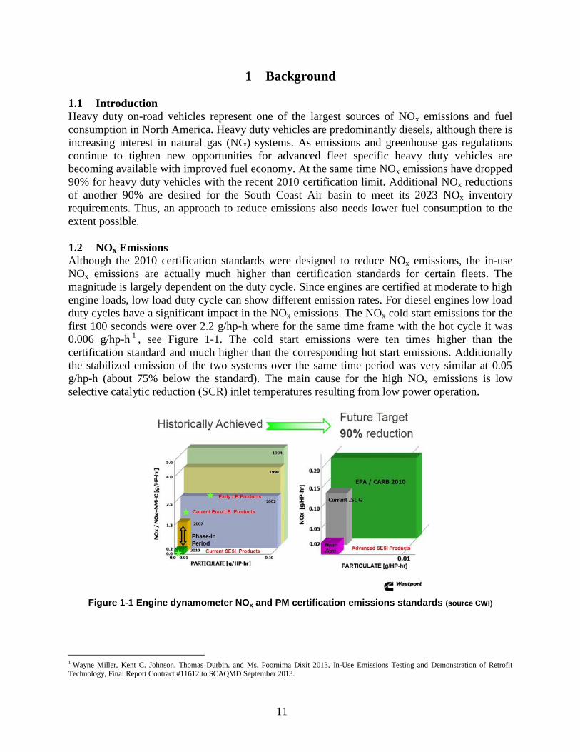
duty cycles have a significant impact in the NOx emissions. The NOx cold start emissions for the

first 100 seconds were over 2.2 g/hp-h where for the same time frame with the hot cycle it was

0.006 g/hp-h1

, see Figure 1-1. The cold start emissions were ten times higher than the

certification standard and much higher than the corresponding hot start emissions. Additionally

the stabilized emission of the two systems over the same time period was very similar at 0.05

g/hp-h (about 75% below the standard). The main cause for the high NOx emissions is low

selective catalytic reduction (SCR) inlet temperatures resulting from low power operation.

Figure 1-1 Engine dynamometer NOx and PM certification emissions standards (source CWI)

1 Wayne Miller, Kent C. Johnson, Thomas Durbin, and Ms. Poornima Dixit 2013, In-Use Emissions Testing and Demonstration of Retrofit Technology, Final Report Contract #11612 to SCAQMD September 2013.

12

These same trucks were tested on cycles designed to simulate port activity2. The port driving

schedule represents near dock (2-6 miles), local (6-20 miles), and regional (20+ miles) drayage

port operation. The SCR was inactive for 100% of the near dock cycle, 95% of the local cycle,

and 60% of the regional cycle, see Figure 1-2. The NOx emissions were on the order of 0.3 to 2

g/hp-h (1 to 9 g/mi) as much as 10 times higher than the 2010 standards. It has been show that

the SCR system also becomes inactive even after hours of operation due to low loads and lean

compression ignition combustion. Thus, the current diesel 2010 solution for low duty cycle

activity (like at ports) is very poor where a NG solution can make significant improvements for

NOx emissions, and a reduction in carbon emissions (carbon dioxide), but at a slight penalty in

equivalent gallon diesel fuel economy.

Figure 1-2 In-use emissions from a heavy duty truck tested on UCR’s chassis dyno

1.3 Fuel economy

Fuel consumption and emissions are a tradeoff due to the science of combustion. Figure 1-3

shows the NOx emissions change with changes in fuel consumption for a typical spark ignited

engine. As NOx is reduced from 0.14 to 0.02 g/hp-h fuel consumption increases a known amount.

This is a result of the stoichiometric combustion of fuels. Advanced catalysts can be used to

reduce NOx from its baseline levels, but trying to reduce NOx within a fixed SI combustion

system will come at a penalty of increased fuel consumption.

Figure 1-3 NOx emissions versus fuel consumption tradeoffs during certification testing

2 Patrick Couch, John Leonard, TIAX Development of a Drayage Truck Chassis Dynamometer Test Cycle, Port of Long Beach/ Contract HD-7188, 2011

(Source CWI)

13

1.4 Objectives

The goals of project are to evaluate the ISL G NZ 8.9 liter ultra-low NOx NG vehicle emissions,

global warming potential, and fuel economy during in-use conditions. Given the low NOx

concentrations expected, additional measures were implemented to quantify NOx emissions at

and below 0.02 g/bhp-hr emissions levels. This report is a summary of the approach, results, and

conclusions of ultra-low NOx NG vehicle evaluation.

14

2 Approach The approach for this demonstration vehicle evaluation includes in-use testing on a chassis

dynamometer, emissions measurements with UCRs mobile emission laboratory (MEL),

improvements to the NOx measurement method and a representative selection of in-use test

cycles. One of the difficulties in quantifying NOx emissions at the levels proposed in this project

(90% lower than the 2010 certification level ~ 0.02 g/bhp-hr) is the measurement methods are

approaching their detection limit to accurately quantify NOx emissions. This section describes

the test article, laboratories and the upgrades performed to quantify NOx emissions at and below

90% of the 2010 emission standard.

2.1 Test article

2.1.1 Engine

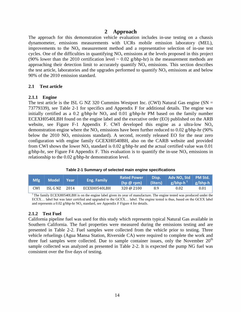
The test article is the ISL G NZ 320 Cummins Westport Inc. (CWI) Natural Gas engine (SN =

73779339), see Table 2-1 for specifics and Appendix F for additional details. The engine was

initially certified as a 0.2 g/bhp-hr NOx and 0.01 g/bhp-hr PM based on the family number

ECEXH0540LBH found on the engine label and the executive order (EO) published on the ARB

website, see Figure F-1 Appendix F. CWI developed this engine as a ultra-low NOx

demonstration engine where the NOx emissions have been further reduced to 0.02 g/bhp-hr (90%

below the 2010 NOx emissions standard). A second, recently released EO for the near zero

configuration with engine family GCEXH0540BH, also on the CARB website and provided

from CWI shows the lower NOx standard is 0.02 g/bhp-hr and the actual certified value was 0.01

g/bhp-hr, see Figure F4 Appendix F. This evaluation is to quantify the in-use NOx emissions in

relationship to the 0.02 g/bhp-hr demonstration level.

Table 2-1 Summary of selected main engine specifications

Mfg Model Year Eng. Family Rated Power (hp @ rpm)

Disp. (liters)

Adv NOx Std g/bhp-h 1

PM Std. g/bhp-h

CWI ISL G NZ 2014 ECEXH0540LBH 320 @ 2100 8.9 0.02 0.01

1 The family ECEXH0540LBH is on the engine label given its year of manufacture. The engine tested was produced under the

ECEX… label but was later certified and upgraded to the GCEX… label. The engine tested is thus, based on the GCEX label

and represents a 0.02 g/bhp-hr NOx standard, see Appendix F Figure 4 for details.

2.1.2 Test Fuel

California pipeline fuel was used for this study which represents typical Natural Gas available in

Southern California. The fuel properties were measured during the emissions testing and are

presented in Table 2-2. Fuel samples were collected from the vehicle prior to testing. Three

vehicle refuelings (Agua Mansa Station, Riverside CA) were required to complete the work and

three fuel samples were collected. Due to sample container issues, only the November 20th

sample collected was analyzed as presented in Table 2-2. It is expected the pump NG fuel was

consistent over the five days of testing.

15

Table 2-2 Fuel properties for the local NG test fuels utilized

Property Molar % Property Molar %

Methane 94.65 Pentane 0.01

Ethane 3.87 Carbon dioxide 0.35

Propane 0.41 Oxygen 0.00

Butane 0.08 Nitrogen 0.63 1 Based on these fuel properties the HHV is 1-42.5 BTU/ft3 and the LHV is 939.9 BTU/ft3 with a H/C ratio of 3.905,

a MON of 132.39 and a carbon weight fraction of 0.745 and a SG = 0.58, see Appendix E for laboratory results. Note

these results meets the US EPA 40 CFR Part 1065.715fuel specification for NG fueled vehicles.

2.1.3 Vehicle inspection

Prior to testing, the vehicle was inspected for proper tire inflation and condition, vehicle

condition, vehicle securing, and the absence of any engine code emission faults. The vehicle

inspection and securing met UCR’s specifications. Cummins Westport Inc. had a service person

on site to make sure fault codes were absent prior to and during emissions testing. All tests were

performed with-in specification and without any engine code faults. Thus, the results presented

in this report are representative of a properly operating vehicle, engine, and aftertreatment

system.

2.1.4 Test cycles

The test vehicle utilized an 8.9 liter NG engine which is available for three typical vocations in

the South Coast Air Basin, 1) goods movement, 2) bus, and 3) refuse3. The engine was provided

to UCR in its refuse hauler application which is one of the more common uses for the 8.9 liter

engine, see Figure 2-4. In order to characterize emissions from this engine over the rage of in-use

applications, goods movement and bus cycles were also tested. UCR tested the vehicle following

the three port cycles (Near Dock, Local, and Regional), the Urban Dynamometer Driving

Schedule (UDDS), the Central Business District (CBD) bus cycle, and the AQMD Refuse cycle,

see Appendix B for details. These cycles are representative of Sothern California driving. Some

cycles are short (less than 15 minutes) where double or triple cycles (2x or 3x) cycles are

recommended in order capture enough PM mass to quantify emissions near 1 mg/bhp-hr. The

UDDS was performed twice (UDDSx2) and the CBD was performed three times (CBDx3)

where the emissions represent the average of the cycle.

Table 4 Summary of statistics for the various proposed driving cycles

Day Distance (mi) Average Speed (mph) Duration (sec) Near Dock 5.61 6.6 3046

Local 8.71 9.3 3362

Regional 27.3 23.2 3661

UDDSx2 11.1 18.8 2122

CBDx3 3.22 20.2 560

AQMD Refuse 4.30 7.31 2997 1 Hot UDDS was performed as a double cycle (2x) and a single (1x) for the cold tests. The CBD was performed as a

triple (3x) test. The refuse cycle includes a compaction element where no distance is accumulated, but emissions are

counted with a simulated compaction cycle, see Appendix B for details.

3 Cummins Westport, California Energy Commission Merit Review- ISL G Near Zero, December 2, 2015

16

2.1.5 Work calculation

The reported emission factors presented are based on a g/bhp-hr and g/mi basis (g/mi are

provided in Appendix E). The engine work is calculated utilizing actual torque, friction torque,

and reference torque from broadcast J1939 ECM signals. The following two formulas show the

calculation used to determine engine brake horse power (bhp) and work (bhp-hr) for the tested

vehicle. Distance is measured by the chassis dynamometer and the vehicle broadcast J1939

vehicle speed signal. A representative ISL G NZ 320 engine lug curve is provided in Figure 2-1.

𝐻𝑝_𝑖 = 𝑅𝑃𝑀_𝑖(𝑇𝑜𝑟𝑞𝑢𝑒𝑎𝑐𝑡𝑢𝑎𝑙_𝑖 − 𝑇𝑜𝑟𝑞𝑢𝑒𝑓𝑟𝑖𝑐𝑡𝑖𝑜𝑛_𝑖)

5252∗ 𝑇𝑜𝑟𝑞𝑢𝑒𝑟𝑒𝑓𝑒𝑟𝑒𝑛𝑐𝑒

Where:

Hp_i instantaneous power from the engine. Negative values set to zero

RPM_i instantaneous engine speed as reported by the ECM (J1939)

Torque_actual_i instantaneous engine actual torque (%): ECM (J1939)

Torque_friction_i instantaneous engine friction torque (%): ECM (J1939)

Torque_reference reference torque (ft-lb) as reported by the ECM (J1939)

𝑊𝑜𝑟𝑘 = ∑𝐻𝑝_𝑖

3600

𝑛

𝑖=0

Figure 2-1 Published ISLG 8.9 Natural Gas engine power curve

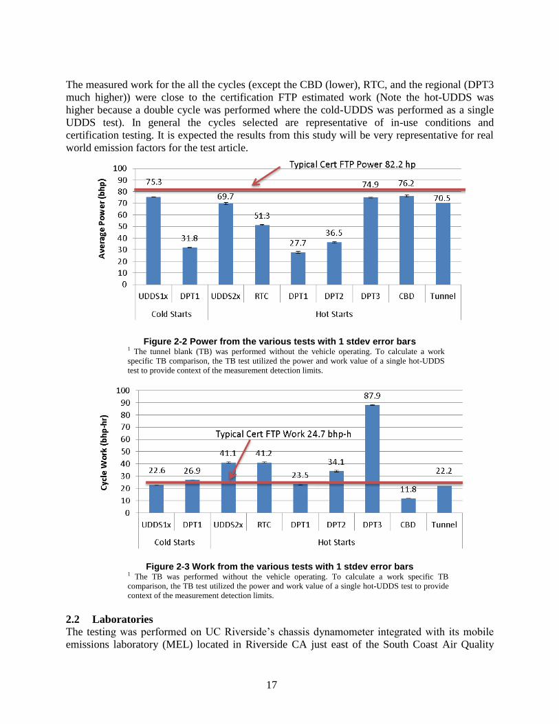
Figure 2-2 and Figure 2-3 show the measured power and work for each of the tests performed on

the refuse vehicle. The engine is certified on the FTP type of cycle where the average power is

around 82 Hp and estimated at 24.7 bhp-h, also shown in Figure 2-2 and Figure 2-3. The UDDS,

regional (DPT3) and the CBD test cycles represent power near (but lower) than the FTP

certification cycle. The near dock (DPT1), local (DPT2), and refuse (RTC) cycles showed much

lower power with the DPT1 being the lowest (as shown by previous studies). Previous testing of

the low power from the DPT1 cycle resulted in high diesel NOx emissions because the SCR

operating temperatures were never obtained.

17

The measured work for the all the cycles (except the CBD (lower), RTC, and the regional (DPT3

much higher)) were close to the certification FTP estimated work (Note the hot-UDDS was

higher because a double cycle was performed where the cold-UDDS was performed as a single

UDDS test). In general the cycles selected are representative of in-use conditions and

certification testing. It is expected the results from this study will be very representative for real

world emission factors for the test article.

Figure 2-2 Power from the various tests with 1 stdev error bars 1 The tunnel blank (TB) was performed without the vehicle operating. To calculate a work

specific TB comparison, the TB test utilized the power and work value of a single hot-UDDS

test to provide context of the measurement detection limits.

Figure 2-3 Work from the various tests with 1 stdev error bars 1 The TB was performed without the vehicle operating. To calculate a work specific TB

comparison, the TB test utilized the power and work value of a single hot-UDDS test to provide

context of the measurement detection limits.

2.2 Laboratories

The testing was performed on UC Riverside’s chassis dynamometer integrated with its mobile

emissions laboratory (MEL) located in Riverside CA just east of the South Coast Air Quality

18

Management District (AQMD). This section describes the chassis dynamometer and emissions

measurement laboratories used for evaluating the in-use emissions from the demonstration

vehicle. Due to challenges of NOx measurement at 0.02 g/bhp-hr, additional sections are

provided to introduce the measurement improvements.

2.2.1 Chassis dynamometer

UCR’s chassis dynamometer is an electric AC type design that can simulate inertia loads from

10,000 lb to 80,000 lb which covers a broad range of in-use medium and heavy duty vehicles,

see Figure 2-4. The design incorporates 48” rolls, vehicle tie down to prevent tire slippage,

45,000 lb base inertial plus two large AC drive motors for achieving a range of inertias. The

dyno has the capability to absorb accelerations and decelerations up to 6 mph/sec and handle

wheel loads up to 600 horse power at 70 mph. This facility was also specially geared to handle

slow speed vehicles such as yard trucks where 200 hp at 15 mph is common. See Appendix D for

more details.

2.2.1.1 Test weight

The ISL G NZ 320 engine is installed in a refuse hauler chassis with a GVW of 62,000 lb, VIN

3BPZX20X6FF100173. The representative test weight for refuse haulers operating in the south

coast air basin is 56,000 lb4. The testing weight of 56,000 lb was also utilized during previous

testing of refuse haulers with diesel and NG engines by UC Riverside and WVU 4 and

5. For this

testing program UCR utilized a testing weight of 56,000 lb for all test cycles (refuse, CBD,

UDDS, and port cycles).

Figure 2-4 UCR’s heavy duty chassis eddy current transient dynamometer

4 Wayne Miller, Kent C. Johnson, Thomas Durbin, and Ms. Poornima Dixit 2014, In-Use Emissions Testing and Demonstration of Retrofit

Technology, Final Report Contract #11612 to SCAQMD September 2014.

5 Daniel K Carder, Mridul Gautam, Arvind Thiruvengada,m Marc C. Besch (2013) In‐Use Emissions Testing and Demonstration of Retrofit

Technology for Control of On‐Road Heavy‐Duty Engines, Final Report Contract #11611 to SCAQMD July 2014.

19

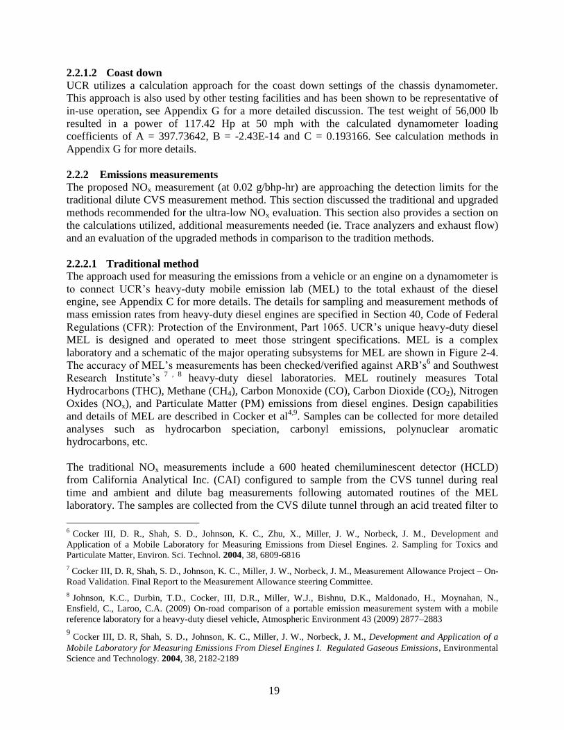
2.2.1.2 Coast down

UCR utilizes a calculation approach for the coast down settings of the chassis dynamometer.

This approach is also used by other testing facilities and has been shown to be representative of

in-use operation, see Appendix G for a more detailed discussion. The test weight of 56,000 lb

resulted in a power of 117.42 Hp at 50 mph with the calculated dynamometer loading

coefficients of A = 397.73642, B = -2.43E-14 and C = 0.193166. See calculation methods in

Appendix G for more details.

2.2.2 Emissions measurements

The proposed NOx measurement (at 0.02 g/bhp-hr) are approaching the detection limits for the

traditional dilute CVS measurement method. This section discussed the traditional and upgraded

methods recommended for the ultra-low NOx evaluation. This section also provides a section on

the calculations utilized, additional measurements needed (ie. Trace analyzers and exhaust flow)

and an evaluation of the upgraded methods in comparison to the tradition methods.

2.2.2.1 Traditional method

The approach used for measuring the emissions from a vehicle or an engine on a dynamometer is

to connect UCR’s heavy-duty mobile emission lab (MEL) to the total exhaust of the diesel

engine, see Appendix C for more details. The details for sampling and measurement methods of

mass emission rates from heavy-duty diesel engines are specified in Section 40, Code of Federal

Regulations (CFR): Protection of the Environment, Part 1065. UCR’s unique heavy-duty diesel

MEL is designed and operated to meet those stringent specifications. MEL is a complex

laboratory and a schematic of the major operating subsystems for MEL are shown in Figure 2-4.

The accuracy of MEL’s measurements has been checked/verified against ARB’s6 and Southwest

Research Institute’s7 , 8

heavy-duty diesel laboratories. MEL routinely measures Total

Hydrocarbons (THC), Methane (CH4), Carbon Monoxide (CO), Carbon Dioxide (CO2), Nitrogen

Oxides (NOx), and Particulate Matter (PM) emissions from diesel engines. Design capabilities

and details of MEL are described in Cocker et al4,9

. Samples can be collected for more detailed

analyses such as hydrocarbon speciation, carbonyl emissions, polynuclear aromatic

hydrocarbons, etc.

The traditional NOx measurements include a 600 heated chemiluminescent detector (HCLD)

from California Analytical Inc. (CAI) configured to sample from the CVS tunnel during real

time and ambient and dilute bag measurements following automated routines of the MEL

laboratory. The samples are collected from the CVS dilute tunnel through an acid treated filter to

6 Cocker III, D. R., Shah, S. D., Johnson, K. C., Zhu, X., Miller, J. W., Norbeck, J. M., Development and

Application of a Mobile Laboratory for Measuring Emissions from Diesel Engines. 2. Sampling for Toxics and

Particulate Matter, Environ. Sci. Technol. 2004, 38, 6809-6816

7 Cocker III, D. R, Shah, S. D., Johnson, K. C., Miller, J. W., Norbeck, J. M., Measurement Allowance Project – On-

Road Validation. Final Report to the Measurement Allowance steering Committee.

8 Johnson, K.C., Durbin, T.D., Cocker, III, D.R., Miller, W.J., Bishnu, D.K., Maldonado, H., Moynahan, N.,

Ensfield, C., Laroo, C.A. (2009) On-road comparison of a portable emission measurement system with a mobile

reference laboratory for a heavy-duty diesel vehicle, Atmospheric Environment 43 (2009) 2877–2883

9 Cocker III, D. R, Shah, S. D., Johnson, K. C., Miller, J. W., Norbeck, J. M., Development and Application of a

Mobile Laboratory for Measuring Emissions From Diesel Engines I. Regulated Gaseous Emissions, Environmental

Science and Technology. 2004, 38, 2182-2189

20

prevent measurement interferences from ammonia (NH3) concentrations. The acid treated filters

were replaced daily.

In addition to the regulated emissions, the laboratory was equipped to measure particle size

distribution (PSD) with TSI’s Engine Exhaust Particle Sizer (EEPS) model 3090, particle

number (PN) with a TSI 3776 condensation particle counter (CPC), soot PM mass with AVL’s

Micro Soot Sensors (MSS 483), NH3 emissions with an integrated real-time tunable diode laser

(TDL) from Unisearch Associates Inc. LasIR S Series, and a batched low level nitrous oxide

(N2O) emissions with a Fourier Transform Infrared Spectrometer (FTIR). The PN measurement

system used a low cut point CPC (2.5 nm D50) because of the large PN concentrations reported

below the PMP protocol CPC 23 nm measurement system (10, 11, and 12). The EEPS

spectrometer displays measurements in 32 channels total (16 channels per decade) and operates

over a wide particle concentration range, including down to 200 particles/cm3.

Figure 2-5 Major Systems within UCR’s Mobile Emission Lab (MEL)

2.2.2.2 NOx Method upgrades

Three NOx upgrade methods were considered for this project. These included 1) real-time raw

sampling and exhaust flow measurements, 2) real-time ambient second by second corrections,

and 3) advanced trace type analyzer bag measurements. The new measurement methods required

instrumentation upgrades which are discussed below.

Raw NOx measurements

The raw NOx measurements utilized a 300 HCLD CAI analyzer which sampled raw exhaust

through a low volume heated filter and heated sample line. The low volume design was

considered to improve the response time of the analyzer with the exhaust flow measurement. The

heated filter was acid treated to minimize NH3 interference with the NOx measurement. A real-

time high speed exhaust flow meter (100 Hz model EFM-HS Sensors Inc) was used to align NOx

21

concentration with real time exhaust flow measurements. The EFM-HS was correlated with UCR

dual CVS system prior to testing to improve the accuracy between the raw and dilute CVS

methods and eliminate exhaust flow biases from propagating through the comparison.

Trace level NOx analyzer

A trace level chemiluminescence NO-NO2-NOx analyzer model 42C manufactured by Thermo

Environmental Instruments Inc (TECO) was used for the real-time ambient measurements and

the low level bag analysis. This analyzer has been operating with-in CE-CERT’s atmospheric

research laboratories for ambient NOx quantification for several years. This analyzer was

calibrated and integrated specially for this ultra-low NOx project. The span on the instrument was

set to 600 ppb and showed a signal to noise ratio about an order in magnitude lower than the

traditional (600 HCLD) analyzer. The signal averaging was reduced from 30 seconds to 1 second

and showed a T10-90 and a T90-10 just over 10 seconds (slightly higher than the specifications of 40

CFR Part 1065). The slightly slower time constant should not impact the gradual transients

expected during real-time ambient measurements or bag concentrations. Although this trace

analyzer does not meet the requirements of 1065, it does provide a good assessment of NOx

emissions below 1 ppm with an ambient trace type NOx analyzer.

2.2.2.3 Calculation upgrades

The calculations for the traditional and improved methods are presented in this section. The

calculations are in agreement with 40 CFR Part 1065, but are presented in a condensed version to

draw observation differences without the details of working in molar flow rates as per 40 CFR

Part 1065.

Table 2-3 NOx measurement methods traditional and upgraded

Type Analyzer Meth. ID Description

Traditional 600 HCLD dil

600 HCLD amb M1 Modal NOx with ambient bag correction

Traditional 600 HCLD dil

600 HCLD amb M2

Dilute bag NOx with ambient bag

correction

Upgrade 300 HCLD raw M3 Raw NOx no ambient bag correction

Upgrade 600 HCLD dil

TECO amb M4

Modal dilute NOx with ambient real

time correction

Upgrade TECO dil

TECO amb M5

Trace analyzer dilute bag with trace

ambient bag correction

Traditional Methods:

The traditional NOx measurement methods are described in the next two equations. The first

equation is the real-time modal measurement corrected for the ambient bag concentration and

real time dilution factor, Method 1 (M1). The second traditional equation (M2) is based on dilute

bag and ambient bag concentrations and an integrated dilution factor over the cycle.

𝑁𝑂𝑥_𝑚1 = ∑(𝑄𝑐𝑣𝑠𝑖∗ ∆𝑡_𝑖) ∗ 𝜌𝑁𝑂𝑥

∗ (𝐶𝑚_𝑖 − 𝐶𝑎 ∗ (1 −1

𝐷𝐹𝑖))

𝑛

𝑖=1

Where:

22

NOx_m1 the Method 1 NOx measurement method (g/cycle)

Qcvs_i is the instantaneous CVS flow

ρNOx is the density of NOx from 40 CFR Part 1065

Cm_i is the instantaneous NOx concentration measured with the dilute NOx 600

HCLD CAI analyzer

Ca is the ambient bag NOx concentration measured by the 600 HCLD CAI

analyzer

DFi instantaneous dilution factor

𝑁𝑂𝑥_𝑚2 = (𝑄𝑐𝑣𝑠_𝑎𝑣𝑒 ∗ ∆𝑡) ∗ 𝜌𝑁𝑂𝑥∗ (𝐶𝑑 − 𝐶𝑎 ∗ (1 −

1

𝐷𝐹_𝑎𝑣𝑒))

Where:


Qcvs_ave is the average CVS flow


Cd is the dilute bag NOx concentration measured with the dilute NOx 600

HCLD CAI analyzer

Ca is the ambient bag NOx concentration measured by the 600 HCLD CAI

analyzer

DFave average dilution factor

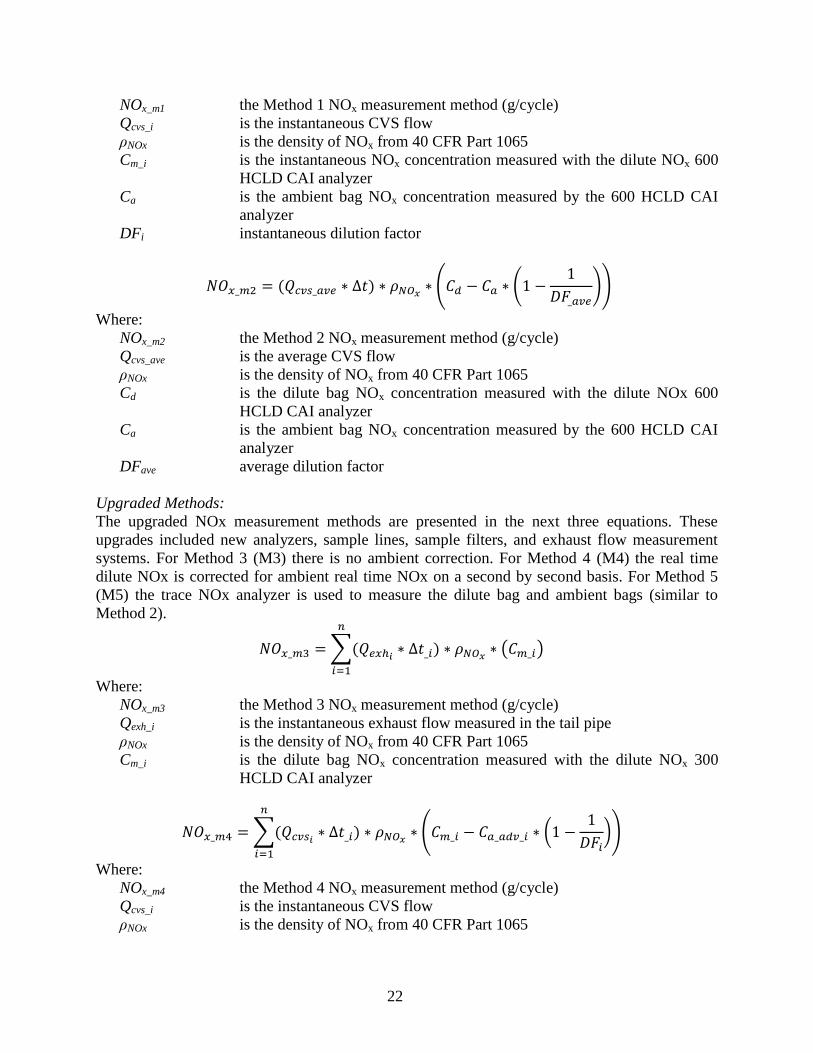
Upgraded Methods:

The upgraded NOx measurement methods are presented in the next three equations. These

upgrades included new analyzers, sample lines, sample filters, and exhaust flow measurement

systems. For Method 3 (M3) there is no ambient correction. For Method 4 (M4) the real time

dilute NOx is corrected for ambient real time NOx on a second by second basis. For Method 5

(M5) the trace NOx analyzer is used to measure the dilute bag and ambient bags (similar to

Method 2).

𝑁𝑂𝑥_𝑚3 = ∑(𝑄𝑒𝑥ℎ𝑖∗ ∆𝑡_𝑖) ∗ 𝜌𝑁𝑂𝑥

∗ (𝐶𝑚_𝑖)

𝑛

𝑖=1

Where:


Qexh_i is the instantaneous exhaust flow measured in the tail pipe


Cm_i is the dilute bag NOx concentration measured with the dilute NOx 300

HCLD CAI analyzer

𝑁𝑂𝑥_𝑚4 = ∑(𝑄𝑐𝑣𝑠𝑖∗ ∆𝑡_𝑖) ∗ 𝜌𝑁𝑂𝑥

∗ (𝐶𝑚_𝑖 − 𝐶𝑎_𝑎𝑑𝑣_𝑖 ∗ (1 −1

𝐷𝐹𝑖))

𝑛

𝑖=1

Where:


Qcvs_i is the instantaneous CVS flow


23

Cm_i is the dilute bag NOx concentration measured with the dilute NOx 600

HCLD CAI analyzer

Ca_adv is the trace ambient bag NOx concentration measured by the TECO trace

NOx analyzer

DFi instantaneous dilution factor

𝑁𝑂𝑥_𝑚5 = (𝑄𝑐𝑣𝑠_𝑎𝑣𝑒 ∗ ∆𝑡) ∗ 𝜌𝑁𝑂𝑥∗ (𝐶𝑑_𝑎𝑑𝑣 − 𝐶𝑎_𝑎𝑑𝑣 ∗ (1 −

1

𝐷𝐹_𝑎𝑣𝑒))

Where:


Qcvs_ave is the average CVS flow


Cd_adv is the dilute bag NOx concentration measured by the TECO trace NOx

analyzer

Ca_adv is the ambient bag NOx concentration measured by the TECO trace NOx

analyzer

DFave average dilution factor

2.2.3 Method evaluation

One of the main contributing factors to the issue with the traditional CVS sampling system is the

magnitude of the ambient concentration has on the calculation. Table 2-4 lists the 10th

, 50th

, and

90th

average ambient, dilute modal, and raw tailpipe measured percentile concentrations. The 50th

percentile raw, dilute, and ambient NOx concentration were 0.55 ppm, 0.17 ppm, and 0.07 ppm

respectively.

As discussed previously, the ambient concentration is subtracted from the dilute concentration

prior to calculating the mass based emissions. This subtraction is typically a larger number minus

a small number. At the 0.02 g/bhp-hr emission level, the ambient concentration is now at the

same levels as the dilute measured value. The ambient concentration was found to be 54% of the

total measured dilute concentration at the 50th

percentile measured concentration, see Table 2-4.

The ambient corrected NOx concentration (Ca_cor) utilized in the dilution measurements is the

product of ambient NOx concentration and an inverse ratio of the dilution factor, see equation

below. If we divide the Ca_cor by the dilute NOx measured we get a ratio that is representative of

the ambient percent of total NOx. Figure 2-6 shows the ratio in a histogram plot and more than

half the data is above 0.6 suggest that most of the measurements meeting the 0.02 g/bhp-hr were

only twice that of ambient concentrations. This ratio gives the reader a feel for the influence

ambient has at and below 0.02 g/bhp-hr NOx emissions.

Table 2-4 Cycle averaged raw, dilute, and ambient measured concentrations (ppm) statistics

Percentile Amb Dilute 1 Raw 1 Ca_cor/Dil %

10th 0.234 0.632 6.533 105%

50th 0.070 0.168 0.554 54%

90th 0.021 0.033 0.070 10%

24

1 With the cold starts removed, the dilute and raw 10th, 50th, and 90th would be 0.326,

0.146, and 0.031 ppm for the dilute concentration and 2.115, 0.450, and 0.069 ppm for

the raw concentration, respectively.

The results show a 10th

, 50th

and 90th

percentile (Ca_cor/Cd) ratio of 10%, 54% and 105%,

respectively. This suggest more than ½ of the measurements were sampled where the dilute

concentration was 50% of the ambient corrected (Ca_cor) concentration. The low concentrations

measured by dilute methods will impact all the methods except for M3 that utilizes the raw

sampling approach where no dilution correction is needed.

𝐶𝑎_𝑐𝑜𝑟 = 𝐶𝑎 ∗ (1 −1

𝐷𝐹_𝑎𝑣𝑒)

Where:

Ca_cor is the ambient NOx concentration factor used in M1

Ca is the ambient bag NOx concentration

DFave cycle average dilution factor (typically 20-30)

(1 −1

𝐷𝐹_𝑎𝑣𝑒) dilution factor term (varied from 0.95 to 0.98 in this study)

Figure 2-6 Ambient fraction of dilute NOx concentration distribution

The real-time concentrations for each cycle is also important where observations suggest a few

NOx spikes of 20-30 times the average values were the basis of the cycle average concentrations.

Section 4 provides additional discussions on the real-time transient NOx measurements. It is

important to understand that the real-time NOx spikes will impact the M1, M3, and M4

measurements since these utilize real-time signals where M2 and M5 are integrated bag signals.

The average mean difference in average emissions between the methods is shown in Table 2-5

with M1 as the reference method. For M2 the average NOx emissions was very similar to M1

(only 5% higher on average, but varied from higher to lower from cycle to cycle). M3 was

slightly lower (-18% on average), but was consistently lower except for the CBD tests. Further

investigation of the CBD tests shows one of the M1 tests had a negative emission rate due a high

ambient bag concentration compared to the modal dilute concentration. This negative value was

25

not an outlier, but a real measurement difficulty at these emission levels. The M4 average NOx

emission rate was notably higher (and relatively more variable) and for M5 the average was

significantly lower for all tests compared to the M1 traditional method.

The M4 utilized real time ambient concentrations for real time correction of the background

calculation. The trace analyzer utilized show some short term drift that didn’t appear to be

related to ambient concentration changes. Additional investigation is needed, but is outside the

scope of this effort. The researchers suggest the M4 method will have more variability as a result

and could be the cause for the higher mean difference.

The M5 utilized the trace NOx analyzer for bag measurements. Surprisingly the M5 method

showed a much lower mean value. Investigations were carried out to see about analyzer drift or

stability and no issues were found during the bag analysis time spans.

Table 2-5 NOx emission average percent difference from Method 1

Trace M2 M3 M4 M5

UDDS1x -17% -40% 96% -87%

DPT1 31% -42% -8% -99%

UDDS2x 7% -13% 21% -70%

RTC 4% -21% 111% -7%

DPT1 -21% -11% 25% -14%

DPT2 3% -20% 25% -61%

DPT3 12% -22% 27% -72%

CBD 19% 23% 32% 16%

Ave 5% -18% 41% -49%

Stdev 17% 20% 40% 42%

A comparison of the statistical significance between the traditional M1 and other methods is

provided in Table 2-6. The two tailed paired t-test and f-test results suggest the two traditional

methods do not have statistically different means or different variances at 95% confidence, see

Table 2-6 (M2 p-value >> 0.05 for both). The upgraded methods showed a different result that

varies. The M3 (raw exhaust flow approach) mean difference is not statistically significant at

95% confidence (M3 p-value > 0.06) but is at the 90% confidence. The M4 (RT ambient

correction) and M5 (trace bag evaluation) upgraded methods both have statistically different

means (p-value < 0.05 for both).

Table 2-6 Comparison to traditional Method 1 measurement (modal dilute NOx)

Method t-test

p-value

f-test

p-value M2 0.521 0.998

M3 0.060 0.152

M4 0.021 0.141

M5 0.001 0.104

26

Each of the added methods (M3, M4, and M5) may have some possible implementation issues

that need to be considered in order to evaluate the comparative results. The M3 measurement

showed good alignment between the measured NOx signal and the exhaust flow signal. The

majority of the NOx mass emissions resulted from a few large spikes, as discussed in Section 4.

These NOx spikes were found to represent more than 80% of the total emission factor. Closer

inspection shows that the NOx concentration and exhaust flow spike occurred simultaneously

and were usually a result of a rapid acceleration from idle.

For the M4 approach (real-time NOx ambient correction) the analyzer had a slight zero stability

issue over the 20-40 minute test cycle not found during the short 3 minute bag analysis. As such,

the drift may be the result of the M4 poor method comparison.

The low M5 method may represent the best approach with very accurate bag measurements for

both the ambient and dilute bag measurements with a trace type NOx analyzer with a larger

sample cell. The drift issue suggested for the M4 measurement didn’t appear to be a factor

during the short bag analysis, but additional tests should be performed to evaluation. As such,

this method may have performed the best, but additional testing is suggested to evaluate this

method on future testing opportunities at 0.02 g/bhp-hr.

In summary the M1, M2, and M3 appear to be the most reliable where the M3 results are more

consistent at the extremely low concentrations measured. M4 and M5 require further

investigation with lower zero drift instrumentation.

27

3 Results

This section describes the results from the ISL G NZ 8.9 liter ultra-low NOx NG engine. The

results are organized by gaseous emissions followed by PM, particle size distribution,

greenhouse gases, and fuel economy. The emission factors presented in g/bhp-hr for comparison

to the certification standard. Emissions in g/mile are provided in Appendix E. Error bars are

represented by single standard deviations due to the relatively large magnitude of the error bars

in relationship to the low emission levels measured for several species (three repeats were

performed where the 95% confidence interval multiplier for the single standard deviation is

3.182).

The UDDS cycle is the representative test cycle for comparisons to the engine certification FTP

cycle where the other cycles (port, refuse, and bus) provide the reader a feel for the in-use

comparability to low duty cycles, cruise conditions, and other vocational specifics of the real

world. As such, the results will be presented in each sub-section within the context of the test

cycle.

3.1 Gaseous emissions

3.1.1 NOx emissions

The NOx emissions are presented in Figure 3-1 for each of the methods evaluated and for all the

test cycles performed. The NOx emissions were below the demonstration 0.02 g/bhp-hr

emissions targets for the UDDS, DPT1 (hot and cold), and the CBD for all measurement

methods. The local and regional port cycles (DPT2 and DPT3) NOx emissions were below the

improved methods but at and below the standard for the traditional methods. The cold start

emissions were higher than the hot tests when comparing between like tests (UDDS cold vs hot

and DPT1 cold vs hot) and averaged at 0.043 g/bhp-hr for the UDDS test cycle (M3).

In general, the NOx emissions are below the ISL G NZ 2016 NOx certification standard of 0.02

g/bhp-hr for all tests and below the in-use NTE standard of 0.03 g/bhp-hr. The reported

certification value listed on the ARB EO is 0.01 g/bhp-hr which is slightly lower than the M3

measurements (0.014 g/bhp-hr) shown for the UDDS hot test cycle, Figure 3-1. Deeper

investigation shows one of the three hot UDDS tests was statistically higher (M3 = 0.009, 0.002,

0.030 g/bhp-hr). A similar trend was also found for the other four methods where the third point

was much higher than the other two points. If the third point was eliminated the average for the

hot UDDS would be just under the EO certification value reported by CWI (M3 = 0.005 g/bhp-

hr). The test-to-test variability shown by the large error bars in Figure 3-1 was investigated

where real-time analysis suggest the variability is not from low measurement issues, but appears

to be the results of the vehicle variability. Section 4 provides a discussion on real-time

investigation.

28

Figure 3-1 Measured NOx emission for the various test cycles

3.1.2 Other gaseous emissions

The hydrocarbon emissions (THC, CH4, and NMHC) are presented in Figure 3-2. The HC are

highest for the cold start tests compared to the hot tests where the regional port cycle (PDT3)

showed the highest HC emissions. For all the hot tests the NMHC was below the standard but

just above the reported certification value except for the regional port cycle. The NMHC was

typically lower than CH4 emission as one would expect for a NG fueled vehicle. The CH4

emissions are lower than the certification results presented in Appendix F Figure F-4 (0.04 vs the

FEL level of 0.65 g/bhp-hr). Also the CH4 emissions for the refuse hauler are significantly lower

(6.4 g/mi vs 0.26 g/mi) than previously tested NG reuse haulers with the 2010 certified NG 8.9

liter engine. The lower CH4 emissions may be a result of the closed crankcase ventilation (CCV)

improvement over previous versions of this engine, see Appendix F for details.

29

Figure 3-2 Hydrocarbon emission factors (g/bhp-hr)

Figure 3-3 shows the CO emissions on a g/bhp-hr basis and Figure 3-4 shows the un-regulated

NH3 emissions on a g/bhp-hr basis. The CO emissions ranged between 1.3 to 5.3 g/bhp-hr for the

cold start near dock (PDT1) and regional (DPT3) test cycles, respectively. The distance specific

emissions ranged from 4.2 to 24.3 g/mi for the regional (PDT3) and the cold start UDDS test

cycles. Previous testing of the ISG vehicle show similar CO emissions ranging from 14.4 to 19.2

g/mi (CBD and UDDS test cycles and same test weights).

Figure 3-3 CO emission factors (g/bhp-hr)

UDDS1x DPT1 UDDS2x RTC DPT1 DPT2 DPT3 CBD Tunnel

Cold Starts Hot Starts

CH4 0.535 0.558 0.043 0.080 0.263 0.155 0.325 0.114 0.004

NMHC 0.323 0.594 0.003 0.010 0.104 0.050 0.168 0.045 -0.019

THC 0.855 1.147 0.046 0.090 0.366 0.205 0.492 0.159 -0.015

-0.2

0.0

0.2

0.4

0.6

0.8

1.0

1.2

1.4

1.6

1.8

HC

Em

issi

on

s (g

/bh

p-h

r) CH4 NMHC THC

30

The NH3 emissions ranged from 0.43 to 0.94 g/bhp-hr for the hot UDDS and regional (DPT3)

cycles. The distance specific emissions varied from 1.16 g/mi to 5.27 g/mi for the regional and

CBD test cycles. The NH3 emissions are slightly higher than previous ISL G vehicle where the

NH3 ranged from 1.17 to 2.8 g/mi for the UDDS and RTC cycle as compared to 1.19 and 4.09

g/mi for the ISL G NZ, respectively. The NH3 concentration varied from 118 ppm (UDDS) to

305 ppm (CBD), see Figure 3-5.

Figure 3-4 Ammonia emission factors (g/bhp-hr)

1 NH3 measurements for the cold UDDS test stopped working during the first hill where the system may

have over ranged. The cold start UDDS NH3 results are estimated at 20% higher than the hot-UDDS test.

Figure 3-5 Ammonia measured tail pipe concentration (ppm)

1 NH3 measurements for the cold UDDS test stopped working during the first hill where the system may

have over ranged. The cold start UDDS NH3 results are estimated at 20% higher than the hot-UDDS test.

3.2 PM emissions

The PM emissions for all the tests including the cold start tests was typically 90% below the

certification standard and close to UCR tunnel blank value of 0.42 g/bhp-hr (based on UDDS

sample time and work), see Figure 3-6. The first regional PM filter weight was statistically

higher than the other three (80, 21, 20 ug) where it is suggested something may have burned off

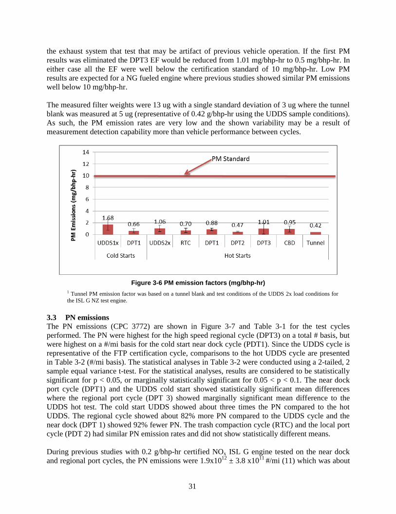
31

the exhaust system that test that may be artifact of previous vehicle operation. If the first PM

results was eliminated the DPT3 EF would be reduced from 1.01 mg/bhp-hr to 0.5 mg/bhp-hr. In

either case all the EF were well below the certification standard of 10 mg/bhp-hr. Low PM

results are expected for a NG fueled engine where previous studies showed similar PM emissions

well below 10 mg/bhp-hr.

The measured filter weights were 13 ug with a single standard deviation of 3 ug where the tunnel

blank was measured at 5 ug (representative of 0.42 g/bhp-hr using the UDDS sample conditions).

As such, the PM emission rates are very low and the shown variability may be a result of

measurement detection capability more than vehicle performance between cycles.

Figure 3-6 PM emission factors (mg/bhp-hr)

1 Tunnel PM emission factor was based on a tunnel blank and test conditions of the UDDS 2x load conditions for

the ISL G NZ test engine.

3.3 PN emissions

The PN emissions (CPC 3772) are shown in Figure 3-7 and Table 3-1 for the test cycles

performed. The PN were highest for the high speed regional cycle (DPT3) on a total # basis, but

were highest on a #/mi basis for the cold start near dock cycle (PDT1). Since the UDDS cycle is

representative of the FTP certification cycle, comparisons to the hot UDDS cycle are presented

in Table 3-2 (#/mi basis). The statistical analyses in Table 3-2 were conducted using a 2-tailed, 2

sample equal variance t-test. For the statistical analyses, results are considered to be statistically

significant for p < 0.05, or marginally statistically significant for 0.05 < p < 0.1. The near dock

port cycle (DPT1) and the UDDS cold start showed statistically significant mean differences

where the regional port cycle (DPT 3) showed marginally significant mean difference to the

UDDS hot test. The cold start UDDS showed about three times the PN compared to the hot

UDDS. The regional cycle showed about 82% more PN compared to the UDDS cycle and the

near dock (DPT 1) showed 92% fewer PN. The trash compaction cycle (RTC) and the local port

cycle (PDT 2) had similar PN emission rates and did not show statistically different means.

During previous studies with 0.2 g/bhp-hr certified NOx ISL G engine tested on the near dock

and regional port cycles, the PN emissions were 1.9x1012

± 3.8 x1011

#/mi (11) which was about

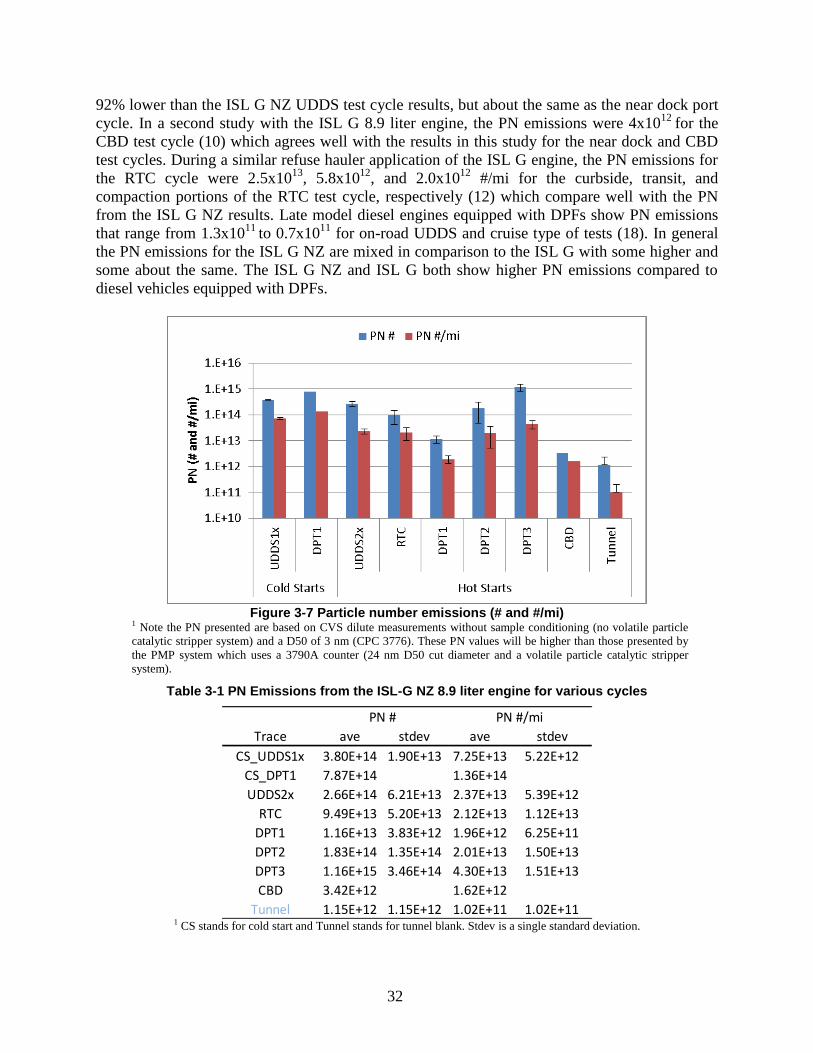
32

92% lower than the ISL G NZ UDDS test cycle results, but about the same as the near dock port

cycle. In a second study with the ISL G 8.9 liter engine, the PN emissions were 4x1012

for the

CBD test cycle (10) which agrees well with the results in this study for the near dock and CBD

test cycles. During a similar refuse hauler application of the ISL G engine, the PN emissions for

the RTC cycle were 2.5x1013

, 5.8x1012

, and 2.0x1012

#/mi for the curbside, transit, and

compaction portions of the RTC test cycle, respectively (12) which compare well with the PN

from the ISL G NZ results. Late model diesel engines equipped with DPFs show PN emissions

that range from 1.3x1011

to 0.7x1011

for on-road UDDS and cruise type of tests (18). In general

the PN emissions for the ISL G NZ are mixed in comparison to the ISL G with some higher and

some about the same. The ISL G NZ and ISL G both show higher PN emissions compared to

diesel vehicles equipped with DPFs.

Figure 3-7 Particle number emissions (# and #/mi)

1 Note the PN presented are based on CVS dilute measurements without sample conditioning (no volatile particle

catalytic stripper system) and a D50 of 3 nm (CPC 3776). These PN values will be higher than those presented by

the PMP system which uses a 3790A counter (24 nm D50 cut diameter and a volatile particle catalytic stripper

system).

Table 3-1 PN Emissions from the ISL-G NZ 8.9 liter engine for various cycles

1 CS stands for cold start and Tunnel stands for tunnel blank. Stdev is a single standard deviation.

Trace ave stdev ave stdev

CS_UDDS1x 3.80E+14 1.90E+13 7.25E+13 5.22E+12

CS_DPT1 7.87E+14 1.36E+14

UDDS2x 2.66E+14 6.21E+13 2.37E+13 5.39E+12

RTC 9.49E+13 5.20E+13 2.12E+13 1.12E+13

DPT1 1.16E+13 3.83E+12 1.96E+12 6.25E+11

DPT2 1.83E+14 1.35E+14 2.01E+13 1.50E+13

DPT3 1.16E+15 3.46E+14 4.30E+13 1.51E+13

CBD 3.42E+12 1.62E+12

Tunnel 1.15E+12 1.15E+12 1.02E+11 1.02E+11

PN # PN #/mi

33

Table 3-2 Statistical comparison to the UDDSx2 test cycle

1 Unpaired two tailed sample equal variance t-test and mean % difference from the UDDSx2 test cycle

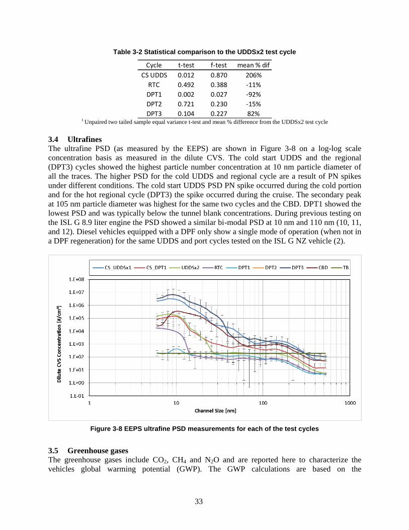
3.4 Ultrafines

The ultrafine PSD (as measured by the EEPS) are shown in Figure 3-8 on a log-log scale

concentration basis as measured in the dilute CVS. The cold start UDDS and the regional

(DPT3) cycles showed the highest particle number concentration at 10 nm particle diameter of

all the traces. The higher PSD for the cold UDDS and regional cycle are a result of PN spikes

under different conditions. The cold start UDDS PSD PN spike occurred during the cold portion

and for the hot regional cycle (DPT3) the spike occurred during the cruise. The secondary peak

at 105 nm particle diameter was highest for the same two cycles and the CBD. DPT1 showed the

lowest PSD and was typically below the tunnel blank concentrations. During previous testing on

the ISL G 8.9 liter engine the PSD showed a similar bi-modal PSD at 10 nm and 110 nm (10, 11,

and 12). Diesel vehicles equipped with a DPF only show a single mode of operation (when not in

a DPF regeneration) for the same UDDS and port cycles tested on the ISL G NZ vehicle (2).

Figure 3-8 EEPS ultrafine PSD measurements for each of the test cycles

3.5 Greenhouse gases

The greenhouse gases include CO2, CH4 and N2O and are reported here to characterize the

vehicles global warming potential (GWP). The GWP calculations are based on the

Cycle t-test f-test mean % dif

CS UDDS 0.012 0.870 206%

RTC 0.492 0.388 -11%

DPT1 0.002 0.027 -92%

DPT2 0.721 0.230 -15%

DPT3 0.104 0.227 82%

34

intergovernmental panel on climate change (IPCC) values of 25 times CO2 equivalent for CH4

and 298 times CO2 equivalent for nitrous oxide (N2O), IPCC fourth assessment report - 2007.

The global warming potential is provided in Table 3-3 on a g/bhp-hr basis (see Appendix E for

g/mi basis). The CH4 and N2O emissions are low and represent 5% for the cold start tests and

around 1-2% for the hot start tests.

Greenhouse gases from vehicles are also found in PM emissions for their absorption of solar

radiation. The main species of the PM responsible for solar absorption is called black carbon

(BC). BC is a short lived climate forcer and is not grouped with the CO2 equivalent method, and

is treated here separately. UCR quantified the BC emissions (referred to as equivalent black

carbon eBC) from the vehicle with its AVL micro soot sensor 483 (MSS) which measures the

PM soot or eBC. Table 3-3 lists the soot PM for each cycle and the ratio of soot/total PM

emissions. The results suggest less than 10% of the PM measured for all the cycles except the

regional port cycle are BC and during the regional cycle up to 22% of the total PM measured is

BC. Additional analysis showed that the measured average concentration ranged between 2-3

ug/m3 when corrected for water interferences (as reported by manufacturer) the concentration

was~ 1ug for all tests. The low concentrations are at the detection limits of the MSS instrument

and suggests the measured BC cannot be quantified accurately, but may suggest BC is not

significant for the ISL G NZ NG engine.

Table 3-3 Global warming potential for the ISLG NZ vehicle tested (g/bhp-hr)

Trace CO2 CH4 N2O GWP (CO2 eq) CO2 /GWP Soot Soot/PM2.5

UDDS1x 546.8 0.53 0.062 578.5 0.95 0.05 3%

DPT1 627.0 0.56 0.090 667.7 0.94 0.02 3%

UDDS2x 548.9 0.04 - 555.0 0.99 0.06 5%

RTC 577.0 0.08 - 584.0 0.99 0.01 1%

DPT1 649.8 0.26 - 661.4 0.98 0.07 8%

DPT2 597.0 0.16 0.027 608.9 0.98 0.1 22%

DPT3 549.3 0.33 0.024 564.4 0.97 0.01 1%

CBD 576.1 0.11 0.034 589.0 0.98 0.04 4% 1 N20 samples were not collected on the hot UDDS, RTC, and DPT1 due to scheduling details. PM Soot

measurements were near the detection limits of the MSS-483 measurement system. The MSS soot signal was

corrected for a 1 ug/1% water interference factor as reported by AVL.

3.6 Fuel economy

The fuel economy of the NG vehicle is evaluated by comparing the CO2 emissions between

cycles where the higher the CO2 the higher the fuel consumption. CO2 is also regulated by EPA

with a standard as performed with the FTP and SET test cycles. The certification like cycle

(UDDS) showed the lowest CO2 emissions and were below 555 g/bhp-hr (FTP standard) for both

the cold start and hot start tests. The NG vehicle CO2 emissions varied slightly between cycles

where only the near dock cycle (DPT1) showed a statistically higher CO2 emission rate. The

average CO2 for all the cycles was 584 g/bhp-hr, and 565 g/bhp-hr with the PDT1 cycle

removed. The CO2 standard and certification value is 555 g/bhp-hr and 465 g/bhp-hr respectively

for this displacement engine, see Figure F1 Appendix F. The standard is the target and the

certification value is the value measured by the manufacturer. It is suggested the higher in-use

CO2 value (ie in the chassis vs on a test stand) could be a result of additional losses in the chassis

where the certification test occurs with the engine on a test stand.

35

Figure 3-9 CO2 emission factors (g/bhp-hr)

The ISL G-NZ MPG on a diesel gallon equivalent (MPGde) basis (assuming 2863gNG/gallon

diesel (14)) ranges from 4.5 MPGde for the regional port cycle (DPT3) to 2.5 MPGde for the CBD

cycle. During previous testing, the previous ISL G 8.9 L fuel economy was found to be 2365

g/mi on a chassis dynamometer at 56,000 GVW following the UDDS test cycle.

36

4 Discussion This section discusses investigation into the real-time data to characterize the impact of the cold

start and transient NOx emissions.

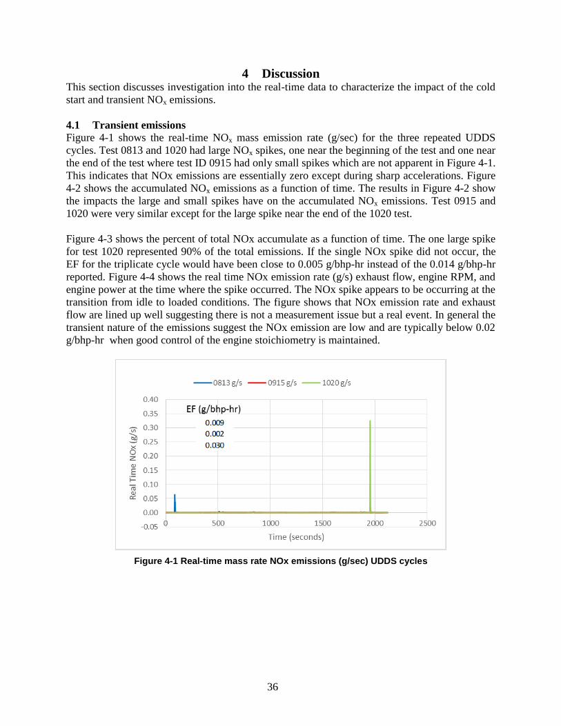
4.1 Transient emissions

Figure 4-1 shows the real-time NOx mass emission rate (g/sec) for the three repeated UDDS

cycles. Test 0813 and 1020 had large NOx spikes, one near the beginning of the test and one near

the end of the test where test ID 0915 had only small spikes which are not apparent in Figure 4-1.

This indicates that NOx emissions are essentially zero except during sharp accelerations. Figure

4-2 shows the accumulated NOx emissions as a function of time. The results in Figure 4-2 show

the impacts the large and small spikes have on the accumulated NOx emissions. Test 0915 and

1020 were very similar except for the large spike near the end of the 1020 test.

Figure 4-3 shows the percent of total NOx accumulate as a function of time. The one large spike

for test 1020 represented 90% of the total emissions. If the single NOx spike did not occur, the

EF for the triplicate cycle would have been close to 0.005 g/bhp-hr instead of the 0.014 g/bhp-hr

reported. Figure 4-4 shows the real time NOx emission rate (g/s) exhaust flow, engine RPM, and

engine power at the time where the spike occurred. The NOx spike appears to be occurring at the

transition from idle to loaded conditions. The figure shows that NOx emission rate and exhaust

flow are lined up well suggesting there is not a measurement issue but a real event. In general the

transient nature of the emissions suggest the NOx emission are low and are typically below 0.02

g/bhp-hr when good control of the engine stoichiometry is maintained.

Figure 4-1 Real-time mass rate NOx emissions (g/sec) UDDS cycles

37

Figure 4-2 Accumulated mass NOx emissions UDDS cycles

Figure 4-3 Real time NOx emissions (percent of total)

-0.2

0.0

0.2

0.4

0.6

0.8

1.0

1.2

0 500 1000 1500 2000 2500

Acc

um

ula

ted

NO

x (%

of

tota

l)

Time (seconds)

0813 % 0915 % 1020 %

38

Figure 4-4 Real time NOx emissions large spike evaluation

4.2 Cold start emissions

Cold start emissions represented a significant part of the total emissions as one would expect.

Figure 4-5 shows the accumulated NOx (g) and exhaust temperature as a function of time. 90%

of the NOx emissions occurred in the first 200 seconds of the cold start test. The remaining part

of the cold UDDS test was very similar to the hot UDDS test. The UDDS hot/cold weighted

emissions is 0.0181 g/bhp-hr (weighted as 1/7th

of the hot cycle). Given that the cold start lasted

200 seconds out of 1080 seconds (total cycle length) the weighted cold start emissions (1/7th

of

the hot test) are, thus, based on 200sec/1080sec/7 = 2.6%. This suggests 2.6% of this vehicles in-

use emissions are represented by a cold start as defined by how the certification process

computes its impact for the regulation process. Also unique to the NG solution, once the catalyst

performance is achieved it remains at this high performance unlike the diesel SCR equipped

engines where low duty cycle will cause the NOx emissions to increase again.

Figure 4-5 Accumulated NOx emissions hot vs cold UDDS comparison

0.00

0.05

0.10

0.15

0.20

0.25

0.30

0.35

0.40

0

200

400

600

800

1000

1200

1400

1600

1800

2000

1920 1930 1940 1950 1960 1970 1980

NO

x Em

issi

on

s (g

/s)

Exh

aust

Flo

w (

scfm

)

Engi

ne

RP

M a

nd

Hp

Time (seconds)

Exh Flow RPM Power NOx g/s

0

100

200

300

400

500

600

0.0

0.1

0.2

0.3

0.4

0.5

0.6

0.7

0.8

0 200 400 600 800 1000

Exh

au

st T

emp

era

ture

(C

)

Acc

um

ula

ted

NO

x (g

)

Time (seconds)

0915 g 0719_CS g

0915 ExhTemp C 0719 ExhTemp C

39

5 Summary and Conclusions

The testing was performed on UC Riverside’s chassis dynamometer integrated with its mobile

emissions laboratory (MEL) located in Riverside CA just east of the South Coast Air Quality

Management District (SCAQMD). The cycles selected for this study are representative of

operation in the South Coast Air Basin and included the urban dynamometer driving schedule,

the near dock, local, and regional port cycles, the AQMD refuse cycle, and the central business

district cycle.

One of the difficulties in quantifying NOx emissions at the levels proposed in this research (90%

below the 2010 certification level ~ 0.02 g/bhp-hr) is the dilute measurement methods are too

close to the detection limit to quantify NOx emissions at the 5% accuracy expected from the

emissions industry. Three upgraded NOx measurement methods were considered which include a

raw NOx measurement integrated with real time exhaust flow, a real-time ambient correction

approach, and a trace level ambient analyzer for accurate bag analysis. In summary the improved

methods varied in their success; however, the raw sampling approach was the most accurate and

precise over the range of conditions tested.

In general the ISL G NZ 8.9 met and exceeded the target NOx emissions of 0.02 g/bhp-hr and

maintained those emissions during a range of duty cycles found in the South Coast Air Basin. It

is expected NG vehicles could play a role in the reduction of the south coast NOx inventory

problem given their near zero emission factors demonstrated

The main conclusions can be summarized as (conclusions are based on the Method 2 results

unless noted otherwise):

1. The ILS G NZ 8.9 liter NG engine showed NOx emissions below the 0.02 g/bhp-hr

emission target and averaged between 0.014 and 0.002 g/bhp-hr for hot start tests.

2. The cold start tests ranged from 0.043 to 0.014 g/bhp-hr for the UDDS and DPT2 cycles.

The UDDS hot/cold weighted emissions was 0.0181 g/bhp-hr for all test cycles

performed which is below the certified 0.02 g/bhp-hr emission factor.

3. The NOx emissions did not increase with lower power duty cycles and showed the

opposite trend where the lower power duty cycles showed lower NOx emissions unlike

the diesel counterparts

4. The large NOx error bars suggest measurement variability, but real-time data shows the

variability is isolated to a few NOx events during rapid tip-in events from accelerations

from idle. This suggests possible driver behavior may impact the overall NOx in-use

performance of the vehicle and more gradual accelerations are desired for minimum

emissions.

5. This suggests possible driver behavior may impact the overall NOx in-use performance of

the vehicle where more gradual accelerations are desired.

6. The other gaseous and PM emissions were similar to previously measured levels from the

0.2 g/bhp-hr ISL G engine and should not add to any unknown impacts for the use of the

NZ engine in the heavy duty fleet.

40

References

1. AQMD 2 October 2015 see: http://www.aqmd.gov/docs/default-

source/Agendas/aqmp/white-paper-working-groups/wp-blueprint-revdf.pdf?sfvrsn=2

2. Wayne Miller, Kent C. Johnson, Thomas Durbin, and Ms. Poornima Dixit 2013, In-Use

Emissions Testing and Demonstration of Retrofit Technology, Final Report Contract

#11612 to SCAQMD December 2013

3. Hesterberg T., Lapin C., Bunn A., Navistar, Inc. 4201 Winfield Road, P.O. Box 1488,

Warrenville, Illinois 60555, VOL. 42, NO. 17, 2008 / ENVIRONMENTAL SCIENCE &

TECHNOLOGY 9 6437

4. Thirubvengadam A., Besch M., Pradhan S., Carder D., and Emission Rates of Regulated

Pollutants from Current Technology Heavy-Duty Diesel and Natural Gas Goods

Movement Vehicles. ENVIRONMENTAL SCIENCE & TECHNOLOGY 2015, 49,

5236−5244

5. Patrick Couch, John Leonard, TIAX Development of a Drayage Truck Chassis

Dynamometer Test Cycle, Port of Long Beach/ Contract HD-7188, 2011.

6. Results from UC Riverside’s Chassis Dyno while testing an 8.9 liter heavy duty vehicle

at transient and state operating modes.

7. Chatterjee, D., Deutschmann, O., and Warnatz, J., Detailed surface reaction mechanism

in a three-way catalyst, Faraday Discussions, 119, pg 371-384 (2001).

8. Cocker III, D. R., Shah, S. D., Johnson, K. C., Zhu, X., Miller, J. W., Norbeck, J. M.,

Development and Application of a Mobile Laboratory for Measuring Emissions from

Diesel Engines. 2. Sampling for Toxics and Particulate Matter, Environ. Sci. Technol.

2004, 38, 6809-6816.

9. Cocker III, D. R, Shah, S. D., Johnson, K. C., Miller, J. W., Norbeck, J. M., Measurement

Allowance Project – On-Road Validation. Final Report to the Measurement Allowance

steering Committee.

10. George Karavalakis, Yu Jiang, Jiacheng Yang, Maryam Hajbabaei, Kent Johnson,

Thomas Durbin, 2016, Gaseous and Particulate Emissions from a Waste Hauler Equipped

with a Stoichiometric Natural Gas Engine on Different Fuel Compositions, SAE

Technical Paper No. 2016-01-0799, Society of Automotive Engineers, World Congress

2016.

11. Hajbabaei, M., Karavalakis, G., Johnson, K.C, Lee, L., and Durbin, T.D., 2013, Impact of

natural gas fuel composition on criteria, toxic, and particle emissions from transit buses

equipped with lean burn and stoichiometric engines, Energy, 62, 425-434.

12. George Karavalakis, Maryam Hajbabaei, Yu Jiang, Jiacheng Yang, Kent C. Johnson,

David R. Cocker; Thomas D. Durbin, 2016, Regulated, Greenhouse Gas, and Particulate

Emissions from Lean-Burn and Stoichiometric Natural Gas Heavy-Duty Vehicles on

Different Fuel Compositions, Fuel, 175, 146-156.

http://www.aqmd.gov/docs/default-source/Agendas/aqmp/white-paper-working-groups/wp-blueprint-revdf.pdf?sfvrsn=2

http://www.aqmd.gov/docs/default-source/Agendas/aqmp/white-paper-working-groups/wp-blueprint-revdf.pdf?sfvrsn=2

41

13. Johnson, K., C., Durbin, T., Khan, Y., M., Jung, H., Cocker, D., (2010). Validation

Testing for the PM-PEMS Measurement Allowance Program. California Air Resources

Board, November 2010, Contract No. 07-620

14. Johnson, K.C., Durbin, T.D., Cocker, III, D.R., Miller, W.J., Bishnu, D.K., Maldonado,

H., Moynahan, N., Ensfield, C., Laroo, C.A. (2009) On-road comparison of a portable

emission measurement system with a mobile reference laboratory for a heavy-duty diesel

vehicle, Atmospheric Environment 43 (2009) 2877–2883

15. Cocker III, D. R, Shah, S. D., Johnson, K. C., Miller, J. W., Norbeck, J. M., Development

and Application of a Mobile Laboratory for Measuring Emissions From Diesel Engines I.

Regulated Gaseous Emissions, Environmental Science and Technology. 2004, 38, 2182-

2189.

16. Miller W., Johnson K., C., Durbin T., Dixit P., (2013) In-Use Emissions Testing and

Demonstration of Retrofit Technology for Control of On-Road Heavy-Duty Engines.

17. L&R Committee 2014 Final Report Appendix A ¬– Items: 232-2, 232-3, 237-1, 237-3,

and 237-5: GGE of Natural Gas as Vehicular Fuel.

18. Zhongqing Zheng, Thomas D. Durbin, Jian Xue, Kent C. Johnson, Yang Li, Shaohua

Hu, Tao Huai, Alberto Ayala, David B. Kittelson, and Heejung S. Jung, Comparison of

Particle Mass and Solid Particle Number (SPN) Emissions from a Heavy-Duty Diesel

Vehicle under On-Road Driving Conditions and a Standard Testing Cycle, Environ. Sci.

Technol. 2014, 48, 1779 – 1786.

42

Appendix A. Test Log

This Appendix contains detailed test logs recorded during engine and chassis dynamometer testing. The testing was performed on

Vehicle ID 2015_016, Project Low NOx 2015, Vehicle VIN = 3BPZX20X6FF100173 with the test mode in Conventional mode. The

chassis and vehicle operators were Eddie and Don for all the testing and the instrument operators were Mark, Jade, Danny and Joey.

Date Test

Time Test Cycle Test ID Hp @ 50 Weight A B C

11/16/2015 14:43 Refuse 201511161358 117.42 56000 397.73642 -2.43E-14 0.193166

11/16/2015 14:56 Compaction Cycle 201511161358 117.42 56000 397.73642 -2.43E-14 0.193166

11/18/2015 7:33 UDDS_CS_1x 201511180727 117.42 56000 397.73642 -2.43E-14 0.193166

11/18/2015 8:17 UDDS_x2 201511180813 117.42 56000 397.73642 -2.43E-14 0.193166

11/18/2015 9:22 UDDS_x2 201511180915 117.42 56000 397.73642 -2.43E-14 0.193166

11/18/2015 10:23 UDDS_x2 201511181020 117.42 56000 397.73642 -2.43E-14 0.193166

11/18/2015 12:14 RTC_DPF_NG 201511181280 117.42 56000 397.73642 -2.43E-14 0.193166

11/19/2015 7:22 UDDS_CS_1x 201511190719 117.42 56000 397.73642 -2.43E-14 0.193166

11/19/2015 7:48 Compaction Cycle warmup 117.42 56000 397.73642 -2.43E-14 0.193166

11/19/2015 8:13 RTC_DPF_NG 201511190809 117.42 56000 397.73642 -2.43E-14 0.193166

11/19/2015 8:54 RTC_DPF_NG 201511190809 117.42 56000 397.73642 -2.43E-14 0.193166

11/19/2015 9:35 RTC_DPF_NG 201511190929 117.42 56000 397.73642 -2.43E-14 0.193166

11/19/2015 10:16 RTC_DPF_NG 201511190929 117.42 56000 397.73642 -2.43E-14 0.193166

11/19/2015 10:58 DTP_1 201511191051 117.42 56000 397.73642 -2.43E-14 0.193166

11/19/2015 12:58 DTP_1 201511191255 117.42 56000 397.73642 -2.43E-14 0.193166

11/19/2015 14:16 DTP_1 201511191412 117.42 56000 397.73642 -2.43E-14 0.193166

11/20/2015 7:19 DTP_1_CS 201511200716 117.42 56000 397.73642 -2.43E-14 0.193166

11/20/2015 8:41 DTP_2 201511200838 117.42 56000 397.73642 -2.43E-14 0.193166

11/20/2015 10:04 DTP_2 201511200959 117.42 56000 397.73642 -2.43E-14 0.193166

11/20/2015 11:24 DTP_2 201511201122 117.42 56000 397.73642 -2.43E-14 0.193166

11/23/2015 7:24 DTP_1_CS 201511230717 117.42 56000 397.73642 -2.43E-14 0.193166

11/23/2015 8:45 DTP_3 201511230840 117.42 56000 397.73642 -2.43E-14 0.193166

11/23/2015 10:18 DTP_3 201511231015 117.42 56000 397.73642 -2.43E-14 0.193166

11/23/2015 12:35 DTP_3 201511231225 117.42 56000 397.73642 -2.43E-14 0.193166

11/23/2015 2:10 CBD 201511231408 117.42 56000 397.73642 -2.43E-14 0.193166

43

Date Test

Time Test Cycle Test ID Hp @ 50 Weight A B C

11/25/2015 8:27 UDDS_CS_1x 201511250820 117.42 56000 397.73642 -2.43E-14 0.193166

11/25/2015 9:13 CBD 201511250907 117.42 56000 397.73642 -2.43E-14 0.193166

11/25/2015 9:48 CBD 201511250946 117.42 56000 397.73642 -2.43E-14 0.193166

44

Appendix B. Test Cycle Description

The test vehicle utilizes an 8.9 liter NG engine which is available for three typical vocations in

the South Coast Air Basin, 1) goods movement, 2) transit bus, and 3) refuse. As such UCR tested

the vehicle following the three drayage type port cycles (Near Dock, Local, and Regional), the

Urban Dynamometer Driving Schedule (UDDS), the Central Business District (CBD) bus cycle,

and the AQMD Refuse cycle. These cycles are representative of Sothern California driving

vocations used. Some cycles are very short (less than 30 minutes) where double or triple cycles

(2x or 3x) cycles are recommended in order capture enough PM mass to quantify emissions near

1 mg/bhp-hr.

Drayage Truck Port (DTP) cycle

TIAX, the Port of Long Beach and the Port of Los Angeles developed the port cycle. Over 1,000

Class 8 drayage trucks at these ports were data logged for trips over a four-week period in 2010.

Five modes were identified based on several driving behaviors: average speed, maximum speed,

energy per mile, distance, and number of stops. These behaviors are associated with different

driving conditions such as queuing or on-dock movement, near-dock, local or regional

movement, and highway movements (see Table B-1 for the phases). The data was compiled and

analyzed to generate a best fit trip (combination of phases). The best-fit trip data was then

additionally filtered (eliminating accelerations over 6 mph/s) to allow operation on a chassis

dynamometer.

The final driving schedule is called the drayage port tuck (DPT) cycle and is represented by 3

modes where each mode has three phases to best represent near dock, local, and regional driving

as shown in Table B-1, B-2 and Figure B-1. The near-dock (DTP-1) cycle is composed of phase

1, 2, and 3a from Table B-1. This gives the complete near-dock cycle listed in Table B-2.

Similarly, for the Local and Regional cycles (DPT-2 and DPT-3) the main difference is phase 3,

which changes to 4 and 5 respectively. Phase 1 and 2 remain the same for all three cycles where

creep and low speed transient are considered common for all the port cycles. For this testing it is

recommended to perform phase 1 through 5 individually and to calculate the weighted emissions

from the combined phases for an overall weighing impact.

Table B-1. Drayage Truck Port cycle by phases

Description Phase

#

Distance

mi

Ave Speed

mph

Max Speed

mph

Cycle

length

Creep

1 0.0274 0.295 4.80 335

low speed

transient 2 0.592 2.67 16.8 798

short high speed

transient 3 4.99 9.39 40.6 1913

Long high

speed transient 4 8.09 13.07 46.4 2229

High speed

cruise 5 24.6 35.04 59.3 2528

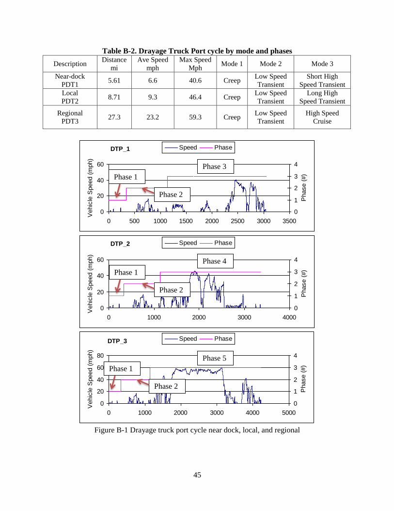
45

Table B-2. Drayage Truck Port cycle by mode and phases

Description Distance

mi

Ave Speed

mph

Max Speed

Mph Mode 1 Mode 2 Mode 3

Near-dock

PDT1 5.61 6.6 40.6 Creep

Low Speed

Transient

Short High

Speed Transient

Local

PDT2 8.71 9.3 46.4 Creep

Low Speed

Transient

Long High

Speed Transient

Regional

PDT3 27.3 23.2 59.3 Creep

Low Speed

Transient

High Speed

Cruise

Figure B-1 Drayage truck port cycle near dock, local, and regional

0

20

40

60

0 500 1000 1500 2000 2500 3000 3500

Vehic

le S

peed (

mph)

0

1

2

3

4

Phase (

#)

Speed PhaseDTP_1

0

20

40

60

0 1000 2000 3000 4000

Vehic

le S

peed (

mph)

0

1

2

3

4

Phase (

#)

Speed PhaseDTP_2

0

20

40

60

80

0 1000 2000 3000 4000 5000

Vehic

le S

peed (

mph)

0

1

2

3

4

Phase (

#)

Speed PhaseDTP_3

Phase 1

Phase 2

Phase 3

Phase 4

Phase 5

Phase 1

Phase 2

Phase 1

Phase 2

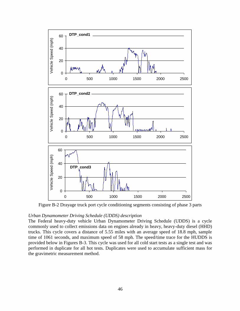
46

Figure B-2 Drayage truck port cycle conditioning segments consisting of phase 3 parts

Urban Dynamometer Driving Schedule (UDDS) description

The Federal heavy-duty vehicle Urban Dynamometer Driving Schedule (UDDS) is a cycle

commonly used to collect emissions data on engines already in heavy, heavy-duty diesel (HHD)

trucks. This cycle covers a distance of 5.55 miles with an average speed of 18.8 mph, sample

time of 1061 seconds, and maximum speed of 58 mph. The speed/time trace for the HUDDS is

provided below in Figures B-3. This cycle was used for all cold start tests as a single test and was

performed in duplicate for all hot tests. Duplicates were used to accumulate sufficient mass for

the gravimetric measurement method.

0

20

40

60

0 500 1000 1500 2000 2500

Vehic

le S

peed (

mph)

DTP_cond1

0

20

40

60

0 500 1000 1500 2000 2500

Vehic

le S

peed (

mph)

DTP_cond2

0

20

40

60

0 500 1000 1500 2000 2500

Vehic

le S

peed (

mph)

DTP_cond3

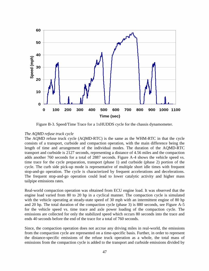
47

Figure B-3. Speed/Time Trace for a 1xHUDDS cycle for the chassis dynamometer.

The AQMD refuse truck cycle

The AQMD refuse truck cycle (AQMD-RTC) is the same as the WHM-RTC in that the cycle

consists of a transport, curbside and compaction operation, with the main difference being the

length of time and arrangement of the individual modes. The duration of the AQMD-RTC

transport and curbside is 2127 seconds, representing a distance of 4.56 miles and the compaction

adds another 760 seconds for a total of 2887 seconds. Figure A-4 shows the vehicle speed vs.

time trace for the cycle preparation, transport (phase 1) and curbside (phase 2) portion of the

cycle. The curb side pick-up mode is representative of multiple short idle times with frequent

stop-and-go operation. The cycle is characterized by frequent accelerations and decelerations.

The frequent stop-and-go operation could lead to lower catalytic activity and higher mass

tailpipe emissions rates.

Real-world compaction operation was obtained from ECU engine load. It was observed that the

engine load varied from 80 to 20 hp in a cyclical manner. The compaction cycle is simulated

with the vehicle operating at steady-state speed of 30 mph with an intermittent engine of 80 hp

and 20 hp. The total duration of the compaction cycle (phase 3) is 880 seconds, see Figure A-5

for the vehicle speed vs. time trace and axle power loading of the compaction cycle. The

emissions are collected for only the stabilized speed which occurs 80 seconds into the trace and

ends 40 seconds before the end of the trace for a total of 760 seconds.

Since, the compaction operation does not accrue any driving miles in real-world, the emissions

from the compaction cycle are represented on a time-specific basis. Further, in order to represent

the distance-specific emissions of the refuse truck operation as a whole, the total mass of

emissions from the compaction cycle is added to the transport and curbside emissions divided by

0

10

20

30

40

50

60

0 100 200 300 400 500 600 700 800 900 1000 1100

Time (sec)

Sp

eed

(m

ph

)

48

the distance of the transport and curbside portion. Thus, it is expected the distance specific

emissions on the refuse cycle will be higher than the transport plus curbside emissions since the

compaction cycle didn’t accumulate any distance.

UCR’s MEL was configured with the conditioning and transport plus triple curbside into a signal

cycle where the sampling was started at second 526 (Start of Transport Phase 1). After

completing Phase 2 (Curbside), the compaction cycle was loaded and the driver brought the

vehicle speed up to 30 mph and then the dyno was put in a load cycle mode that oscillated from

20 to 80 hp as shown in Figure B-5.

Figure B-4 Speed trace for AQMD refuse truck driving cycle

Figure B-5 Speed trace for AQMD refuse truck compaction cycle

0

10

20

30

40

50

60

70

80

90

0

5

10

15

20

25

30

35

0 100 200 300 400 500 600 700 800 900 1000

Hub

Pow

er (H

P)

Spee

d (M

PH)

Speed Power

Simulated Compaction Phase 3

49

Central Business District (CBD) Cycle

The Central Business District (CBD) Cycle is a chassis dynamometer testing procedure for

heavy-duty vehicles (SAE J1376). The CBD cycle represents a “sawtooth” driving pattern, which

includes 14 repetitions of a basic cycle composed of idle, acceleration, cruise, and deceleration

modes. The following are characteristic parameters of the cycle:

Duration: 560 s

Average speed: 20.23 km/h

Maximum speed: 32.18 km/h (20 mph)

Driving distance: 3.22 km

Average acceleration: 0.89 m/s2

Maximum acceleration: 1.79 m/s2

Vehicle speed over the duration of the CBD cycle is shown in Figure A-1.

Figure B-6. CBD Driving Cycle

The standard CBD test cycle will be used for bus testing where three cycles will be combined for

a triple CBD for a total sample time of 30 minutes. Performing the CBD cycle three times in one

test allows for additional sample volumes to be collected for all batched type analysis (filters,

DNPH, BETEX and N2O). Preconditioning is defined as performing a previous triple CBD and a

20 minute soak to improve repeatability between hot repeats. Emissions analyses for gaseous

emissions will also be collected over the triple CBD cycles. This cycle is shown in Figure A-2.

The triple CBD cycle will be repeated in triplicate for repeatability metrics as described earlier.

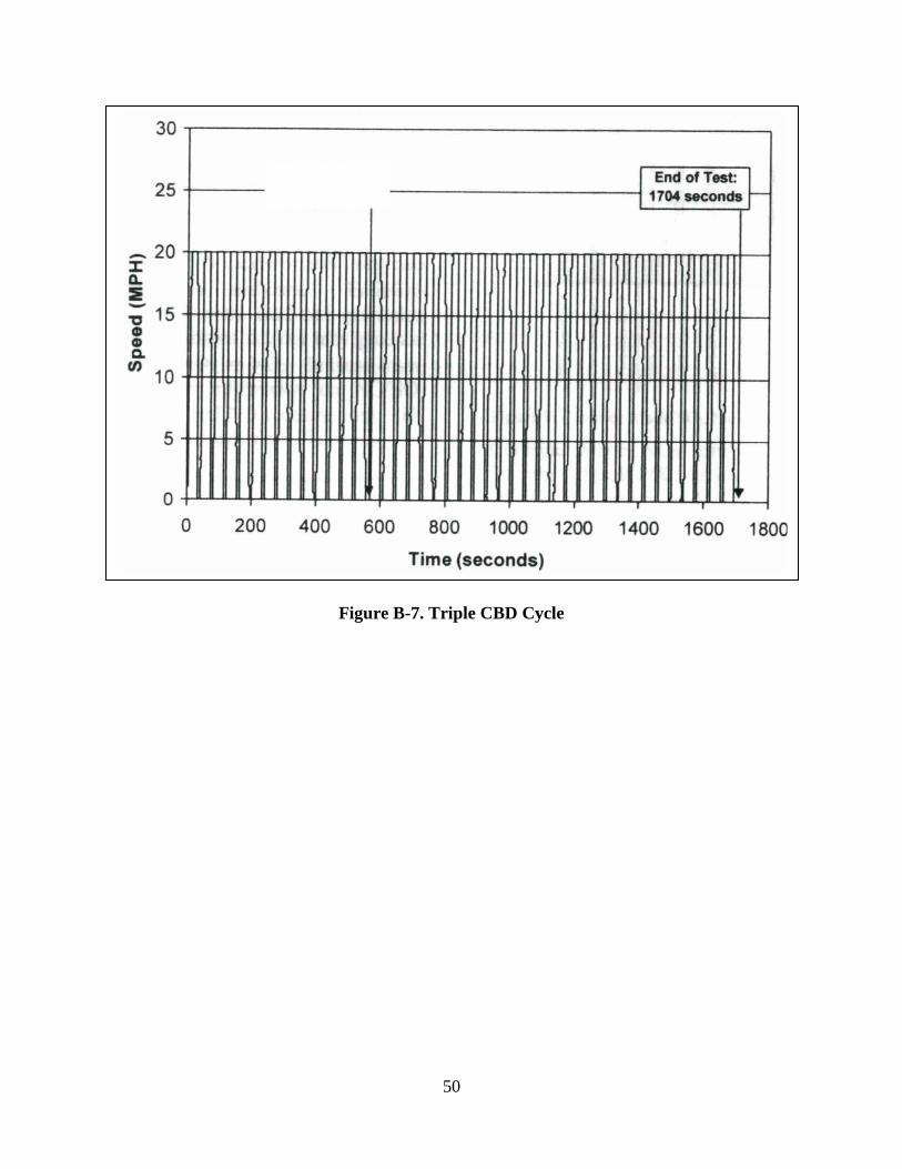
50

Figure B-7. Triple CBD Cycle

51

Appendix C. UCR Mobile Emission Laboratory

The approach used for measuring the emissions from a vehicle or an engine on a dynamometer is

to connect UCR’s heavy-duty mobile emission lab (MEL) to the total exhaust of the diesel

engine. The details for sampling and measurement methods of mass emission rates from heavy-

duty diesel engines are specified in Code of Federal Regulations (CFR): Protection of the

Environment, Section 40, Part 1065. UCR’s unique heavy-duty diesel mobile emissions

laboratory (MEL) is designed and operated to meet those stringent specifications. MEL is a

complex laboratory and a schematic of the major operating subsystems for MEL are shown in

Figure C-1. The accuracy of MEL’s measurements have been checked/verified against ARB’s10

and Southwest Research Institute’s11,12

heavy-duty diesel laboratories. MEL routinely measures

Total Hydrocarbons (THC), Methane, Carbon Monoxide, Carbon Dioxide, Nitrogen Oxides, and

Particulate Matter (PM) emissions from diesel engines. Design capabilities and details of MEL

are described in Cocker et al1,13

. Samples can be collected for more detailed analyses such as

hydrocarbon speciation, carbonyl emissions, polynuclear aromatic hydrocarbons, etc.

Figure C-1: Major Systems within UCR’s Mobile Emission Lab (MEL)

10

Cocker III, D. R., Shah, S. D., Johnson, K. C., Zhu, X., Miller, J. W., Norbeck, J. M., Development and

Application of a Mobile Laboratory for Measuring Emissions from Diesel Engines. 2. Sampling for Toxics and

Particulate Matter, Environ. Sci. Technol. 2004, 38, 6809-6816

11 Cocker III, D. R, Shah, S. D., Johnson, K. C., Miller, J. W., Norbeck, J. M., Measurement Allowance Project –

On-Road Validation. Final Report to the Measurement Allowance steering Committee.

12 Johnson, K.C., Durbin, T.D., Cocker, III, D.R., Miller, W.J., Bishnu, D.K., Maldonado, H., Moynahan, N.,

Ensfield, C., Laroo, C.A. (2009) On-road comparison of a portable emission measurement system with a mobile

reference laboratory for a heavy-duty diesel vehicle, Atmospheric Environment 43 (2009) 2877–2883

13 Cocker III, D. R, Shah, S. D., Johnson, K. C., Miller, J. W., Norbeck, J. M., Development and Application of a

Mobile Laboratory for Measuring Emissions From Diesel Engines I. Regulated Gaseous Emissions, Environmental

Science and Technology. 2004, 38, 2182-2189

52

Appendix D. Heavy-Duty Chassis Dynamometer Laboratory

UCR’s chassis dynamometer is an electric AC type design that can simulate inertia loads from

10,000 lb to 80,000 lb which covers a broad range of in-use medium and heavy duty vehicles,

see Figure D-1. The design incorporates 48” rolls, axial loading to prevent tire slippage, 45,000

lb base inertial plus two large AC drive for achieving a range of inertias. The dyno has the

capability to absorb accelerations and decelerations up to 6 mph/sec and handle wheel loads up

to 600 horse power at 70 mph. This facility was also specially geared to handle slow speed

vehicles such as yard trucks where 200 hp at 15 mph is common.

The chassis dynamometer was designed to accurately perform the new CARB 4 mode cycle,

urban dynamometer driving schedule (UDDS), refuse drive schedule (WHM), bus cycles (CBD),

as well as any speed vs time trace that do not exceed the acceleration and deceleration rates. The

load measurement uses state of the art sensing and is accurate to 0.05% FS and has a response

time of less than 100 ms which is necessary for repeatable and accurate transient testing. The

speed accuracy of the rolls is ± 0.01 mph and has acceleration accuracy of ± 0.02 mph/sec which

are both measured digitally and thus easy to maintain their accuracy. The torque transducer is

calibrated as per CFR 1065 and is a standard method used for determining accurate and reliable

wheel loads.

Figure D-1. UCR’s heavy duty chassis eddy current transient dynamometer

53

Mustang Publication “Project Spotlights” March 2010

54

55

Appendix E. Additional Test Data and Results

This appendix includes some additional results not presented in the main report, but can be used to support the assumptions and

decisions made for the results presented. Following Tables E-1 through E-4 are fuel sample analysis reports.

Table E-1 Average emission factors for all cycles (g/bhp-hr)

Duration Engine Ave Modal Emission Factor (g/bhp-hr) PM (mg/bhp-hr) NOx Emissions (mg/bhp-hr)

Trace sec bhp bhp-hr THC CH4 NMHC CO N2O CO2 NH3 PM2.5 Soot M1 M2 M3 M4 M5

CS_UDDS 1081 75.3 22.6 0.85 0.53 0.32 4.28 0.062 546.8

1.7 0.05 51.5 48.0 43.5 70.7 34.1

CS_DPT1 3049 31.8 26.9 1.15 0.56 0.59 5.25 0.090 627.0 0.64 0.7 0.02 22.5 28.6 14.0 20.9 2.7

UDDS 2122 69.7 41.1 0.05 0.04 0.00 1.51 - 548.9 0.32 1.1 0.06 16.6 18.0 13.9 20.9 2.6

RTC 2889 51.3 41.2 0.09 0.08 0.01 2.75 - 577.0 0.44 0.7 0.00 6.4 7.2 2.2 28.6 4.9

DPT1 3049 27.7 23.5 0.37 0.26 0.10 2.35 - 649.8 0.66 0.9 0.07 4.2 0.0 2.0 9.2 1.4

DPT2 3365 36.5 34.1 0.20 0.16 0.05 2.01 0.027 597.0 0.47 0.5 0.10 16.6 17.2 12.6 21.6 4.5

DPT3 4228 74.9 87.9 0.49 0.33 0.17 1.34 0.024 549.3 0.37 1.0 0.01 18.4 20.8 14.1 23.7 4.1

CBD 560 76.2 11.8 0.16 0.11 0.05 2.73 0.034 576.1 0.94 0.9 0.04 -3.3 0.4 1.2 3.1 -0.2

Tunnel 1134 70.5 22.2 -0.01 0.00 -0.02 -0.07 0.5 0.03 0.4 0.04 0.2 2.6 1.0 1.4 0.6

Table E-2 Standard deviation of the emission factors for all cycles (g/bhp-hr)

Duration Engine Stdev Modal Emission Factor (g/bhp-hr) PM (mg/bhp-hr) NOx Emissions (mg/bhp-hr)


CS_UDDS 0.0 0.2 0.1 0.07 0.04 0.03 0.39 - 14.1

0.9 0.01 26.9 32.3 11.7 17.5 29.2

CS_DPT1 0.0 0.1 0.1 0.52 0.08 0.44 0.71 - 2.9 0.09 0.4 0.07 24.4 19.2 8.7 4.7 0.9

UDDS 0.0 1.1 0.6 0.01 0.01 0.01 0.13 - 9.1 0.01 0.5 0.03 20.1 21.6 15.1 22.8 3.5

RTC 0.0 0.4 0.3 0.05 0.03 0.03 0.44 - 8.1 0.08 0.4 0.10 5.1 2.9 1.3 45.9 8.6

DPT1 0.0 1.1 0.9 0.20 0.13 0.07 0.39 - 8.3 0.12 0.2 0.02 4.1 7.8 1.9 2.8 0.4

DPT2 0.0 0.7 0.6 0.03 0.01 0.01 0.06 0.004 13.7 0.02 0.1 0.01 10.8 10.7 6.3 12.5 0.8

DPT3 0.0 0.3 0.4 0.03 0.02 0.01 0.23 0.003 7.7 0.10 0.9 0.01 4.7 6.5 3.6 6.5 1.9

CBD 0.0 0.8 0.1 0.02 0.02 0.01 0.75 0.012 25.9 0.24 0.5 0.01 6.3 1.0 1.3 1.5 0.3

Tunnel - - - - - - - - - - - - - - - - -

56

Table E-3 Average emission factors for all cycles (g/mi)

Vehicle Ave Modal Emission Factor (g/mi) PM (mg/mi) NOx Emissions (mg/mi)

Trace sec bhp mi THC CH4 NMHC CO N2O CO2 NH3 PM2.5 Soot M1 M1 M1 M1 M1

CS_UDDS 1081 75.3 5.2 3.70 2.31 1.40 18.5 0.27 2367 - 7.3 0.21 223 208 189 306 164

CS_DPT1 3049 31.8 5.8 5.29 2.58 2.74 24.3 0.41 2895 2.98 3.1 0.10 104 132 65 96 13

UDDS 2122 69.7 11.2 0.17 0.16 0.01 5.5 - 2005 1.19 3.9 0.20 61 66 51 77 10

RTC 2889 51.3 4.4 0.82 0.74 0.09 25.4 - 5348 4.09 6.5 0.02 61 67 20 274 47

DPT1 3049 27.7 5.9 1.45 1.04 0.41 9.4 - 2589 2.64 3.5 0.29 17 -1 8 37 6

DPT2 3365 36.5 9.1 0.77 0.58 0.19 7.5 0.10 2236 1.77 1.7 0.39 63 65 48 81 17

DPT3 4228 74.9 28.1 1.54 1.02 0.53 4.2 0.07 1718 1.16 3.2 0.05 58 65 44 74 13

CBD 560 76.2 2.1 0.89 0.64 0.25 15.3 0.19 3226 5.27 5.3 0.23 -19 2 7 17 0

Tunnel 1134 70.5 6.0 -0.07 0.02 -0.08 -0.3 - 1.9 0.10 1.6 0.14 1 10 4 5 2

Table E-4 Standard deviation of the emission factors for all cycles (g/mi)

Vehicle Stdev Modal Emission Factor (g/mi) PM (mg/mi) NOx Emissions (mg/mi)


CS_UDDS 0 0.2 0.1 0.22 0.13 0.09 1.4 - 93 - 4.2 0.06 118 141 53 79 156

CS_DPT1 0 0.1 0.0 2.37 0.37 2.02 3.4 - 3 0.39 1.6 0.35 112 88 40 22 4

UDDS 0 1.1 0.1 0.05 0.03 0.02 0.4 - 8 0.06 2.0 0.12 75 81 56 85 13

RTC 0 0.4 0.1 0.44 0.26 0.23 3.4 - 146 0.78 3.2 0.96 49 30 12 444 83

DPT1 0 1.1 0.1 0.77 0.50 0.28 2.0 - 88 0.61 0.6 0.08 17 31 7 11 2

DPT2 0 0.7 0.1 0.11 0.06 0.05 0.3 0.01 16 0.11 0.3 0.04 41 41 24 47 3

DPT3 0 0.3 0.1 0.08 0.04 0.04 0.7 0.01 27 0.31 2.8 0.04 14 20 11 20 6

CBD 0 0.8 0.0 0.14 0.10 0.05 4.4 0.07 187 1.44 3.1 0.04 36 5 7 9 0

Tunnel - - - - - - - - - - - - - - - - -

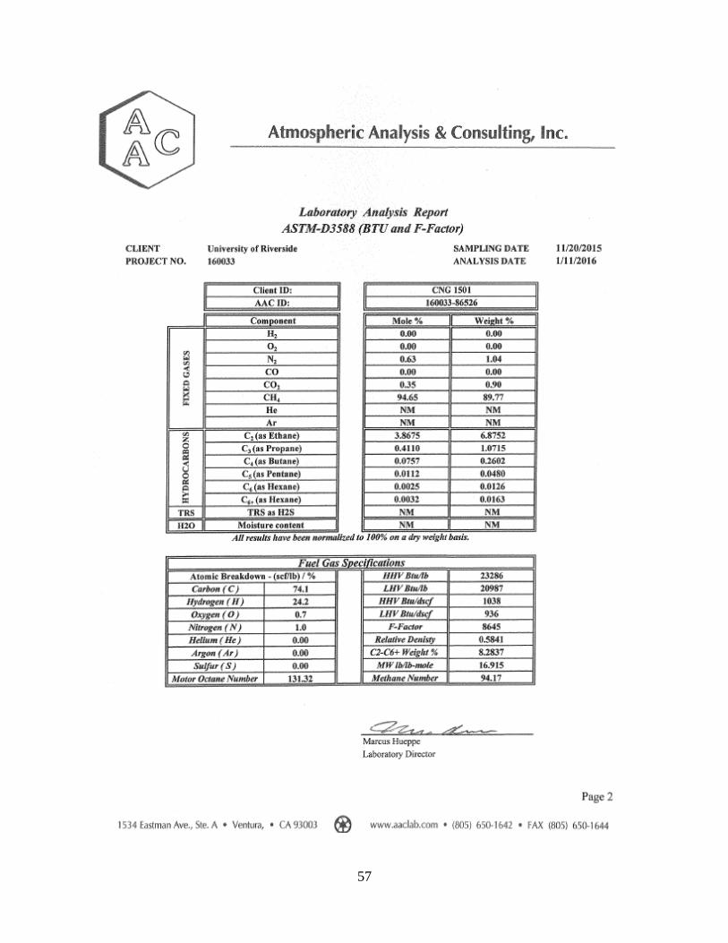
57

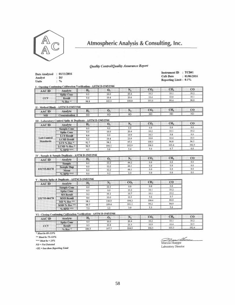
58

59

60

Appendix F. Engine certification data, labels, and upgrades

This appendix includes the engine executive order Figure F-1 as listed on the ARB website for

the family number listed on the engine name plate see Figure F-2 and F-3, Family number

ECEXH0540LBH. The ISL G NZ certification is provided in the recently released documents as

presented in Figure F-4, 5, and 6.

Figure F-1 Engine certification order for the ISL G (not ISL G NZ) NG engine (ARB

source)

61

Figure F-2 Engine label for the ISL G NZ 320 NG engine

Figure F-3 Engine label for the ISL G NZ 320 NG engine

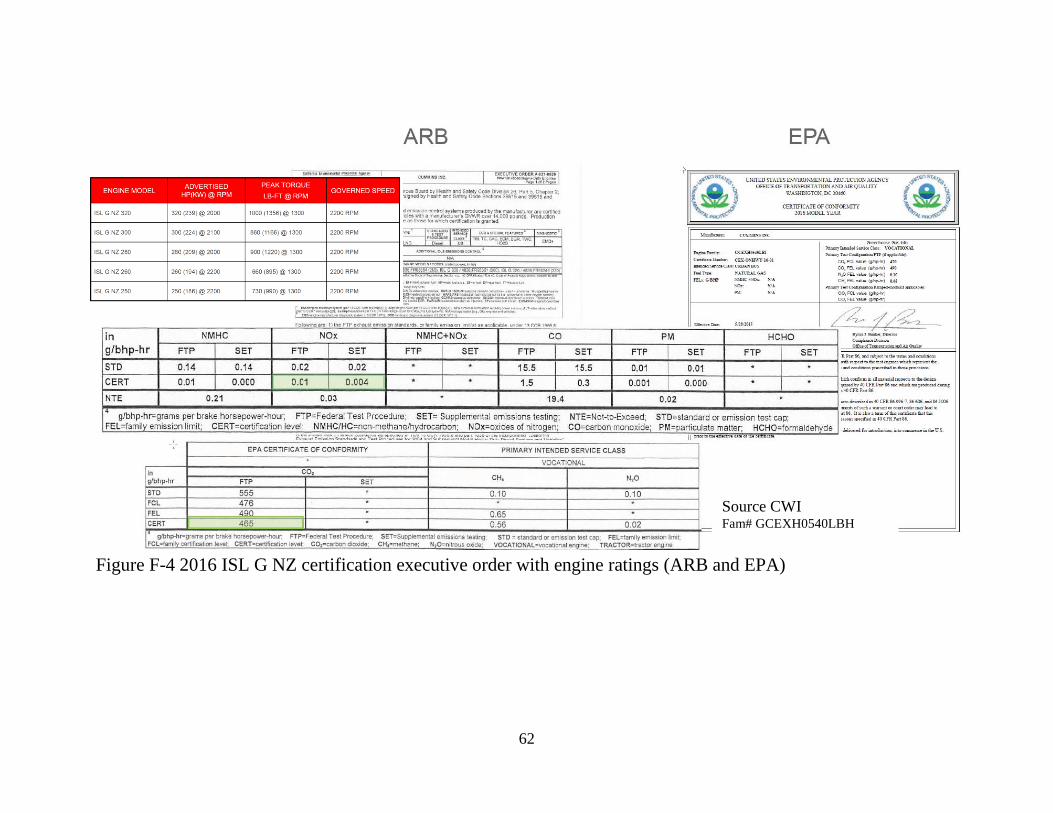
62

Figure F-4 2016 ISL G NZ certification executive order with engine ratings (ARB and EPA)

Source CWI Fam# GCEXH0540LBH

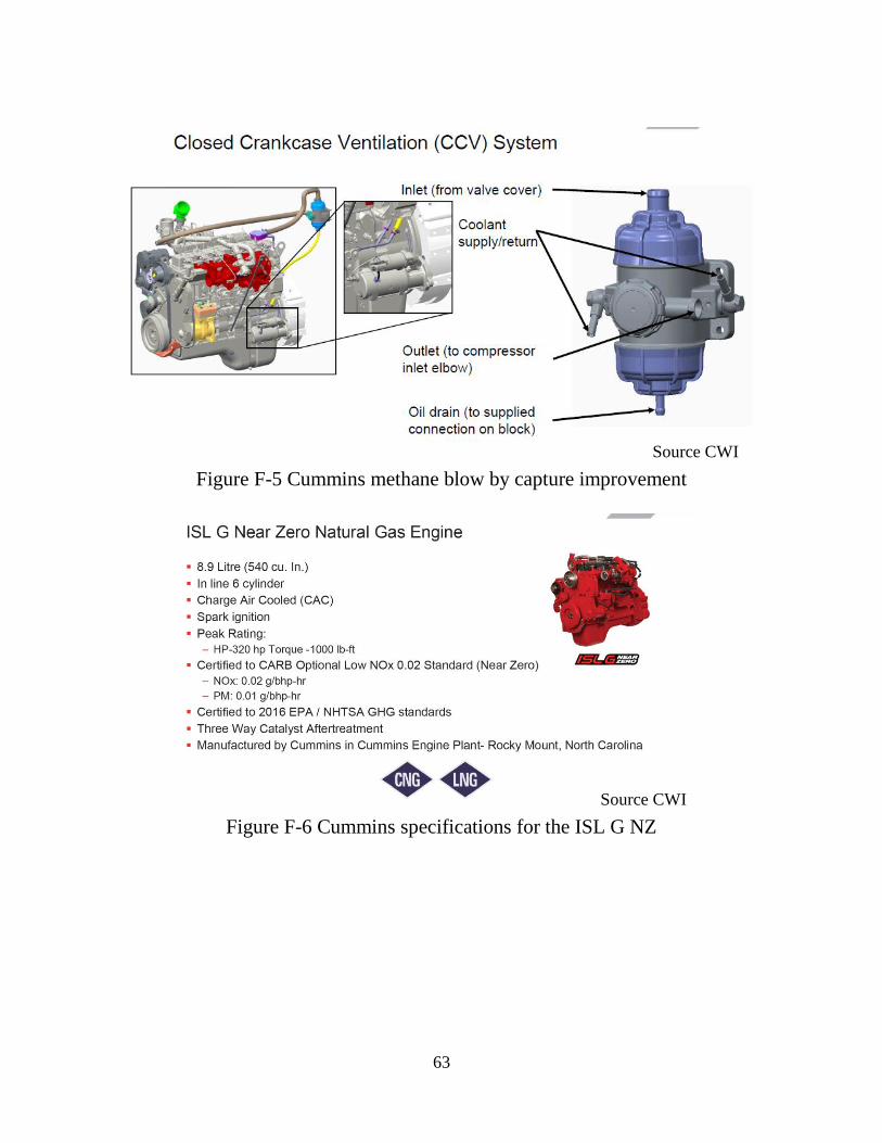
63

Figure F-5 Cummins methane blow by capture improvement

Figure F-6 Cummins specifications for the ISL G NZ

Source CWI

Source CWI

64

Figure F-7 ISL G NZ emission enhancements

Source CWI

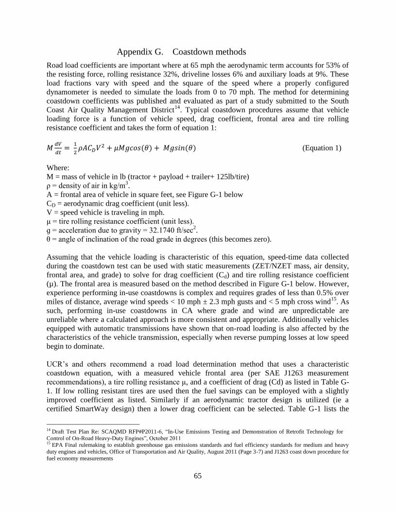
65

Appendix G. Coastdown methods

Road load coefficients are important where at 65 mph the aerodynamic term accounts for 53% of

the resisting force, rolling resistance 32%, driveline losses 6% and auxiliary loads at 9%. These

load fractions vary with speed and the square of the speed where a properly configured

dynamometer is needed to simulate the loads from 0 to 70 mph. The method for determining

coastdown coefficients was published and evaluated as part of a study submitted to the South

Coast Air Quality Management District14

. Typical coastdown procedures assume that vehicle

loading force is a function of vehicle speed, drag coefficient, frontal area and tire rolling

resistance coefficient and takes the form of equation 1:

𝑀𝑑𝑉

𝑑𝑡=

1

2𝜌𝐴𝐶𝐷𝑉2 + 𝜇𝑀𝑔𝑐𝑜𝑠(𝜃) + 𝑀𝑔𝑠𝑖𝑛(𝜃) (Equation 1)

Where:

M = mass of vehicle in lb (tractor + payload + trailer+ 125lb/tire)

ρ = density of air in kg/m3.

A = frontal area of vehicle in square feet, see Figure G-1 below

CD = aerodynamic drag coefficient (unit less).

V = speed vehicle is traveling in mph.

μ = tire rolling resistance coefficient (unit less).

ɡ = acceleration due to gravity = 32.1740 ft/sec2.

θ = angle of inclination of the road grade in degrees (this becomes zero).

Assuming that the vehicle loading is characteristic of this equation, speed-time data collected

during the coastdown test can be used with static measurements (ZET/NZET mass, air density,

frontal area, and grade) to solve for drag coefficient (Cd) and tire rolling resistance coefficient

(µ). The frontal area is measured based on the method described in Figure G-1 below. However,

experience performing in-use coastdowns is complex and requires grades of less than 0.5% over

miles of distance, average wind speeds < 10 mph ± 2.3 mph gusts and < 5 mph cross wind15

. As

such, performing in-use coastdowns in CA where grade and wind are unpredictable are

unreliable where a calculated approach is more consistent and appropriate. Additionally vehicles

equipped with automatic transmissions have shown that on-road loading is also affected by the

characteristics of the vehicle transmission, especially when reverse pumping losses at low speed

begin to dominate.

UCR’s and others recommend a road load determination method that uses a characteristic

coastdown equation, with a measured vehicle frontal area (per SAE J1263 measurement

recommendations), a tire rolling resistance μ, and a coefficient of drag (Cd) as listed in Table G-

1. If low rolling resistant tires are used then the fuel savings can be employed with a slightly

improved coefficient as listed. Similarly if an aerodynamic tractor design is utilized (ie a

certified SmartWay design) then a lower drag coefficient can be selected. Table G-1 lists the

14 Draft Test Plan Re: SCAQMD RFP#P2011-6, “In-Use Emissions Testing and Demonstration of Retrofit Technology for

Control of On-Road Heavy-Duty Engines”, October 2011 15 EPA Final rulemaking to establish greenhouse gas emissions standards and fuel efficiency standards for medium and heavy

duty engines and vehicles, Office of Transportation and Air Quality, August 2011 (Page 3-7) and J1263 coast down procedure for

fuel economy measurements

66

coefficients to use based on different ZET/NZET configurations. Once the coefficients are

selected then they can be used in the above equation to calculate coastdown times to be used for

calculating the A, B, C coefficients in Equation 2 for the dynamometer operation parameters.

From these equations calculate the coastdown times from based on the coefficients in Table G-1

as shown in Table G-2 (65,000 lb, ustd, Cdstd and Table G-1). From Table G-2 one can plot the

force (lb) vs average speed bin to get the ABC coefficients for the chassis dynamometer (see

Figure G-2). These are the coefficients to enter into the chassis dynamometer then validate via

the details of Appendix C. Repeat process until validation criteria is met. Typically one or two

iterations is needed to meet the validation criteria.

Table G-1 Constants and parameters for Class 8 heavy duty trucks

Variable Value Description

θ 0 no grade in these tests

ρ 1.202 standard air density kg/m3

μstd 0.00710 standard tires

μadv 0.00696 low rolling resistant tires

CD_std 0.750 for non-SmartWay tractor

CD_adv 0.712 for SmartWay tractor

ɡ 9.806 nominal value m/sec2

M Varies mass: final test weight kg 1 The tire rolling resistance, μ, for low rolling resistant tires shows a 1-2% savings (ref SmartWay). As such utilize

0.00686 fpr low rolling resistant tires. In this document the tractors may vary, but the trailers will be assumed

similar. As such, if the tractor utilizes the certified SmartWay tractor type then coefficient of drag can be reduced

by up to 10% (5% fuel savings) depending on the technology. As such in this guidance document utilize the

Cd_adv for SmartWay tractors and Cd_std for non-SmartWay tractors. Additionally, for reference other vocations

show higher Cd’s, such as the CD = 0.79 for buses and 0.80 for refuse trucks. Nominal value of gravity is used in

this document where actual value can be found by following 40CFR 1065.630 or at http://www.ngs.noaa.gov

𝑑𝑉

𝑑𝑡=

1

2

𝜌𝐴𝐶𝐷𝑉2

𝑀+ 𝜇𝑔𝑐𝑜𝑠(𝜃) + 𝑔𝑠𝑖𝑛(𝜃) (Equation 2)

http://www.ngs.noaa.gov/

67

Figure G-1 Vehicle frontal area dimensions method

Using Equation 2 (solution for 𝑑𝑉

𝑑𝑡 or deceleration), one can calculate the deceleration for each

average speed bin (60, 50, … down to 20 mph), see Table G-2. From the deceleration time one

can calculate the desired time which is the target for the coast down simulation on the chassis

dynamometer. Using the final test weight (M), the total simulated force can be calculated using

Equation 1 at each speed bin, see values Table G-2. Plot the simulated force (lb) on the y-axis vs

truck speed (mph) on the x-axis. Using a best fit polynomial of order two, calculate the

polynomial coefficients A (0th

order term), B (1st order term), and C (2

nd order term), see Figure

G-2. Enter these ABCs into your chassis dynamometer and verify the coast down times match

your desired coast down times to within 5%.

The calculation approach is consistent and has proven very reliable for chassis testing heavy duty

vehicle and has been used for years by UCR and others. For detailed evaluation of aerodynamic

modifications and body styles, UCR recommends investing the time perform in-use coastdowns

where sufficient program resources will be needed as per 40 CFR Part 1066, SAE J2263, and

J1263.

Table G-2 Desired coastdown times for a Class 8 truck with standard components

Avg Speed Calc Time Decel Decel Decel Force

Data Point MPH sec MPH/Sec ft/sec2

Gs lb

65-55 60 25.67 0.38954 0.57 0.018 1154

55-45 50 31.44 0.31806 0.47 0.014 942

45-35 40 38.51 0.25965 0.38 0.012 769

35-25 30 46.68 0.21422 0.31 0.010 635

25-15 20 55.02 0.18177 0.27 0.008 539

Desired

68

Figure G-2 Resulting ABCs based on Table G-2 results

Documents

Ultra-Low NOx Natural Gas Vehicle Evaluation ISL G NZ CWI LowNOx NG_Finalv06.pdf · Final Report Ultra-Low NO x Natural Gas Vehicle Evaluation ISL G NZ November 2016 Submitted by: