Embed Size (px)
Citation preview
arX
iv:1
501.
0350
6v2
[ast
ro-p
h.H
E]
17 A
pr 2
015
Astronomy & Astrophysicsmanuscript no. cdfs˙grpcat˙arxiv c© ESO 2015April 20, 2015
Ultra-deep catalog of X-ray groups in the Extended Chandra D eepField South
A. Finoguenov1,2, M. Tanaka3, M. Cooper4, V. Allevato1, N. Cappelluti5,2, A. Choi6, C. Heymans6, F.E. Bauer7,8,9, F.Ziparo10, P. Ranalli11,5, J. Silverman12, W.N. Brandt13, Y. Q. Xue14, J. Mulchaey15, L. Howes16,24, C. Schmid17, D.
Wilman25,16, A. Comastri5, G. Hasinger18, V. Mainieri19, B. Luo20, P. Tozzi21, P. Rosati22, P. Capak23, and P. Popesso16
1 Department of Physics, University of Helsinki, Gustaf Hallstromin katu 2a, FI-00014 Helsinki, Finland2 University of Maryland Baltimore County, 1000 Hilltop circle, Baltimore, MD 21250, USA3 National Astronomical Observatory of Japan 2-21-1 Osawa, Mitaka, Tokyo 181-8588, Japan4 Center for Galaxy Evolution, Department of Physics and Astronomy, University of California, Irvine, 4129 Frederick Reines Hall
Irvine, CA 92697 USA5 INAF-Osservatorio Astronomico di Bologna, Via Ranzani 1, I-40127 Bologna, Italy6 Scottish Universities Physics Alliance, Institute for Astronomy, University of Edinburgh, Royal Observatory, Blackford Hill,
Edinburgh EH9 3HJ, UK7 Instituto de Astrofısica, Facultad de Fısica, PontificiaUniversidad Catolica de Chile, 306, Santiago 22, Chile8 Millennium Institute of Astrophysics9 Space Science Institute, 4750 Walnut Street, Suite 205, Boulder, Colorado 80301
10 School of Physics and Astronomy, University of Birmingham,Edgbaston, Birmingham B15 2TT, UK11 IAASARS, National Observatory of Athens, GR-15236 Penteli, Greece12 Institute for the Physics and Mathematics of the Universe, University of Tokyo, Kashiwa 2778582, Japan13 Department of Astronomy & Astrophysics, 525 Davey Lab, The Pennsylvania State University, University Park, PA 16802, USA14 Key Laboratory for Research in Galaxies and Cosmology, Center for Astrophysics, Department of Astronomy, University of
Science and Technology of China, Chinese Academy of Sciences, Hefei, Anhui 230026, China15 Observatories of the Carnegie Institution, 813 Santa Barbara Street, Pasadena, CA 91101, USA16 Max-Planck-Institut fuer extraterrestrische Physik, Giessenbachstrasse 1, D-85748 Garching, Germany17 Dr. Karl Remeis-Observatory & ECAP, University Erlangen-Nuremberg, Sternwartstr. 7, 96049 Bamberg, Germany18 Institute for Astronomy, 2680 Woodlawn Drive Honolulu, HI 96822-1839 USA19 European Southern Observatory, Karl-Schwarzschild-Strasse 2, Garching D-85748, Germany20 Harvard-Smithsonian Center for Astrophysics, 60 Garden Street, Cambridge, MA 02138, USA21 INAF - Osservatorio Astrofisico di Firenze, Largo E. Fermi 5,50125 Firenze, Italy22 Dipartimento di Fisica e Scienze della Terra, Universita degli Studi di ‘ Ferrara, Via Saragat 1, I-44122 Ferrara, Italy23 California Institute of Technology, MS 249-17 Pasadena, CA91125, USA24 Research School of Astronomy & Astrophysics, Australian National University, Cotter Road, Weston Creek, ACT 2611, Australia25 Universitatssternwarte Munchen, Scheinerstrasse 1, 8167 9 Muunchen, Germany
Published online: 17 April 2015
ABSTRACT
Aims. We present the detection, identification and calibration ofextended sources in the deepest X-ray dataset to date, the extendedChandra Deep Field South (ECDF-S).Methods. Ultra-deep observations of ECDF-S with Chandra and XMM-Newton enable a search for extended X-ray emission downto an unprecedented flux of 2× 10⁻¹⁶ ergs s−1 cm−2. By using simulations and comparing them with the Chandra and XMM data, weshow that it is feasible to probe extended sources of this fluxlevel, which is 10,000 times fainter than the first X-ray group catalogs ofthe ROSAT all sky survey. Extensive spectroscopic surveys at the VLT and Magellan have been completed, providing spectroscopicidentification of galaxy groups to high redshifts. Furthermore, available HST imaging enables a weak-lensing calibration of the groupmasses.Results. We present the search for the extended emission on spatial scales of 32′′ in both Chandra and XMM data, covering 0.3 squaredegrees and model the extended emission on scales of arcminutes. We present a catalog of 46 spectroscopically identifiedgroups,reaching a redshift of 1.6. We show that the statistical properties of ECDF-S, such as logN-logS and X-ray luminosity function arebroadly consistent with LCDM, with the exception that dn/dz/dΩ test reveals that a redshift range of 0.2 < z < 0.5 in ECDF-S issparsely populated. The lack of nearby structure, however,makes studies of high-redshift groups particularly easierboth in X-raysand lensing, due to a lower level of clustered foreground. Wepresent one and two point statistics of the galaxy groups as well asweak-lensing analysis to show that the detected low-luminosity systems are indeed low-mass systems. We verify the applicabilityof the scaling relations between the X-ray luminosity and the total mass of the group, derived for the COSMOS survey to lowermasses and higher redshifts probed by ECDF-S by means of stacked weak lensing and clustering analysis, constraining anypossibledepartures to be within 30% in mass.Conclusions. Ultra-deep X-ray surveys uniquely probe the low-mass galaxy groups across a broad range of redshifts. These groupsconstitute the most common environment for galaxy evolution. Together with the exquisite data set available in the beststudied partof the Universe, the ECDF-S group catalog presented here hasan exceptional legacy value.
Key words. galaxy groups – galaxy evolution
1
1. Introduction
Detection of extended X-ray emission is an important sourceofinformation on the hot intergalactic medium of groups and clus-ters of galaxies. A sample of X-ray groups recovered by deepsurveys is a unique resource to improve our understanding oflow-mass groups as well as distant clusters. It also provides in-formation on the common environment of massive galaxies.
The advent of Chandra and XMM-Newton has ele-vated galaxy group research to a new level, with largecatalogs of X-ray selected groups now available for manysurveys (Finoguenov et al. 2007, 2010, 2009; George et al.2011; Adami et al. 2011; Connelly et al. 2012; Erfanianfar etal.2013). The first studies using those catalogs have already re-vealed substantial differences in the galaxy population of galaxygroups: compared to galaxy clusters, groups have more baryonslocked in galaxies (Giodini et al. 2009), and have more star-forming galaxies (Giodini et al. 2012; Popesso et al. 2012).Theredshift evolution of the star-formation rate in groups hasbeenfound to differ from clusters, approaching the field level at inter-mediate redshifts (Popesso et al. 2012). Diversity of the opticalproperties of high-z groups has been reported by Tanaka et al.(2013b).
The ability of X-rays to characterise galaxy groups in termsof their mass and virial radius enables a robust separation ofmass and radial trends in galaxy formation. Ziparo et al. (2014)showed that a fundamental difference exists between X-ray de-tected groups and group-like density regions, where environ-mental processes related to a massive dark matter halo are moreefficient in quenching galaxy star formation with respect topurely density related processes. In particular, the rapidevo-lution of galaxies in groups with respect to group-like densityregions and the field highlights the leading role of X-ray de-tected groups in the cosmic quenching of star formation. Useof groups provides a direct estimate of the halo occupation dis-tribution, which are not affected by the sample variance, as wellas to separate the contribution from central and satellite galaxies(Smolcic et al. 2011; George et al. 2011, 2012; Leauthaud et al.2012; Allevato et al. 2012; Oh et al. 2014).
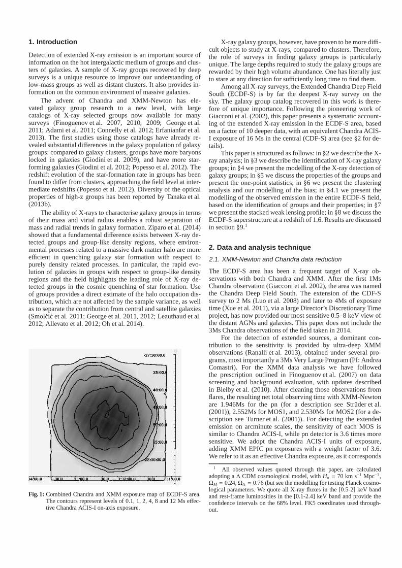
Fig. 1: Combined Chandra and XMM exposure map of ECDF-S area.The contours represent levels of 0.1, 1, 2, 4, 8 and 12 Ms effec-tive Chandra ACIS-I on-axis exposure.
X-ray galaxy groups, however, have proven to be more diffi-cult objects to study at X-rays, compared to clusters. Therefore,the role of surveys in finding galaxy groups is particularlyunique. The large depths required to study the galaxy groupsarerewarded by their high volume abundance. One has literally justto stare at any direction for sufficiently long time to find them.
Among all X-ray surveys, the Extended Chandra Deep FieldSouth (ECDF-S) is by far the deepest X-ray survey on thesky. The galaxy group catalog recovered in this work is there-fore of unique importance. Following the pioneering work ofGiacconi et al. (2002), this paper presents a systematic account-ing of the extended X-ray emission in the ECDF-S area, basedon a factor of 10 deeper data, with an equivalent Chandra ACIS-I exposure of 16 Ms in the central (CDF-S) area (see§2 for de-tails).
This paper is structured as follows: in§2 we describe the X-ray analysis; in§3 we describe the identification of X-ray galaxygroups; in§4 we present the modelling of the X-ray detection ofgalaxy groups; in§5 we discuss the properties of the groups andpresent the one-point statistics; in§6 we present the clusteringanalysis and our modelling of the bias; in§4.1 we present themodelling of the observed emission in the entire ECDF-S field,based on the identification of groups and their properties; in §7we present the stacked weak lensing profile; in§8 we discuss theECDF-S superstructure at a redshift of 1.6. Results are discussedin section§9.1
2. Data and analysis technique
2.1. XMM-Newton and Chandra data reduction
The ECDF-S area has been a frequent target of X-ray ob-servations with both Chandra and XMM. After the first 1MsChandra observation (Giacconi et al. 2002), the area was namedthe Chandra Deep Field South. The extension of the CDF-Ssurvey to 2 Ms (Luo et al. 2008) and later to 4Ms of exposuretime (Xue et al. 2011), via a large Director’s DiscretionaryTimeproject, has now provided our most sensitive 0.5–8 keV view ofthe distant AGNs and galaxies. This paper does not include the3Ms Chandra observations of the field taken in 2014.
For the detection of extended sources, a dominant con-tribution to the sensitivity is provided by ultra-deep XMMobservations (Ranalli et al. 2013), obtained under severalpro-grams, most importantly a 3Ms Very Large Program (PI: AndreaComastri). For the XMM data analysis we have followedthe prescription outlined in Finoguenov et al. (2007) on datascreening and background evaluation, with updates describedin Bielby et al. (2010). After cleaning those observations fromflares, the resulting net total observing time with XMM-Newtonare 1.946Ms for the pn (for a description see Struder et al.(2001)), 2.552Ms for MOS1, and 2.530Ms for MOS2 (for a de-scription see Turner et al. (2001)). For detecting the extendedemission on arcminute scales, the sensitivity of each MOS issimilar to Chandra ACIS-I, while pn detector is 3.6 times moresensitive. We adopt the Chandra ACIS-I units of exposure,adding XMM EPIC pn exposures with a weight factor of 3.6.We refer to it as an effective Chandra exposure, as it corresponds
1 All observed values quoted through this paper, are calculatedadopting aΛ CDM cosmological model, withHo = 70 km s−1 Mpc−1,ΩM = 0.24,ΩΛ = 0.76 (but see the modelling for testing Planck cosmo-logical parameters. We quote all X-ray fluxes in the [0.5-2] keV bandand rest-frame luminosities in the [0.1-2.4] keV band and provide theconfidence intervals on the 68% level. FK5 coordinates used through-out.
A. Finoguenov et al.: Ultra-deep catalog of X-ray groups in the Extended Chandra Deep Field South
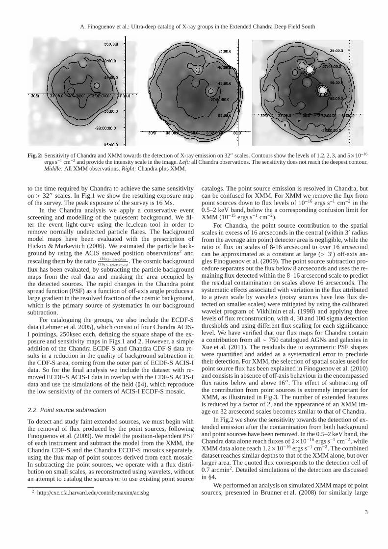
Fig. 2: Sensitivity of Chandra and XMM towards the detection of X-ray emission on 32′′ scales. Contours show the levels of 1.2, 2,3, and 5×10⁻¹⁶
ergs s−1 cm−2 and provide the intensity scale in the image.Left: all Chandra observations. The sensitivity does not reach the deepest contour.Middle: All XMM observations.Right:Chandra plus XMM.
to the time required by Chandra to achieve the same sensitivityon > 32′′ scales. In Fig.1 we show the resulting exposure mapof the survey. The peak exposure of the survey is 16 Ms.
In the Chandra analysis we apply a conservative eventscreening and modelling of the quiescent background. We fil-ter the event light-curve using the lcclean tool in order toremove normally undetected particle flares. The backgroundmodel maps have been evaluated with the prescription ofHickox & Markevitch (2006). We estimated the particle back-ground by using the ACIS stowed position observations2 andrescaling them by the ratiocts9.5−12keV,data
cts9.5−12keV,stowed. The cosmic background
flux has been evaluated, by subtracting the particle backgroundmaps from the real data and masking the area occupied bythe detected sources. The rapid changes in the Chandra pointspread function (PSF) as a function of off-axis angle produces alarge gradient in the resolved fraction of the cosmic background,which is the primary source of systematics in our backgroundsubtraction.
For cataloguing the groups, we also include the ECDF-Sdata (Lehmer et al. 2005), which consist of four Chandra ACIS-I pointings, 250ksec each, defining the square shape of the ex-posure and sensitivity maps in Figs.1 and 2. However, a simpleaddition of the Chandra ECDF-S and Chandra CDF-S data re-sults in a reduction in the quality of background subtraction inthe CDF-S area, coming from the outer part of ECDF-S ACIS-Idata. So for the final analysis we include the dataset with re-moved ECDF-S ACIS-I data in overlap with the CDF-S ACIS-Idata and use the simulations of the field (§4), which reproducethe low sensitivity of the corners of ACIS-I ECDF-S mosaic.
2.2. Point source subtraction
To detect and study faint extended sources, we must begin withthe removal of flux produced by the point sources, followingFinoguenov et al. (2009). We model the position-dependent PSFof each instrument and subtract the model from the XMM, theChandra CDF-S and the Chandra ECDF-S mosaics separately,using the flux map of point sources derived from each mosaic.In subtracting the point sources, we operate with a flux distri-bution on small scales, as reconstructed using wavelets, withoutan attempt to catalog the sources or to use existing point source
2 http://cxc.cfa.harvard.edu/contrib/maxim/acisbg
catalogs. The point source emission is resolved in Chandra,butcan be confused for XMM. For XMM we remove the flux frompoint sources down to flux levels of 10−16 ergs s−1 cm−2 in the0.5–2 keV band, below the a corresponding confusion limit forXMM (10−15 ergs s−1 cm−2).
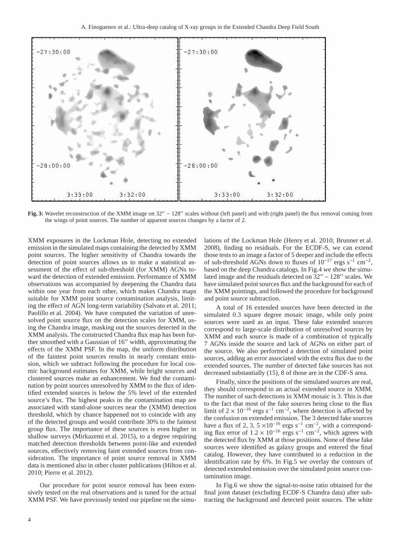
For Chandra, the point source contribution to the spatialscales in excess of 16 arcseconds in the central (within 3′ radiusfrom the average aim point) detector area is negligible, while theratio of flux on scales of 8-16 arcsecond to over 16 arcsecondcan be approximated as a constant at large (> 3′) off-axis an-gles Finoguenov et al. (2009). The point source subtractionpro-cedure separates out the flux below 8 arcseconds and uses the re-maining flux detected within the 8–16 arcsecond scale to predictthe residual contamination on scales above 16 arcseconds. Thesystematic effects associated with variation in the flux attributedto a given scale by wavelets (noisy sources have less flux de-tected on smaller scales) were mitigated by using the calibratedwavelet program of Vikhlinin et al. (1998) and applying threelevels of flux reconstruction, with 4, 30 and 100 sigma detectionthresholds and using different flux scaling for each significancelevel. We have verified that our flux maps for Chandra containa contribution from all∼ 750 catalogued AGNs and galaxies inXue et al. (2011). The residuals due to asymmetric PSF shapeswere quantified and added as a systematical error to precludetheir detection. For XMM, the selection of spatial scales used forpoint source flux has been explained in Finoguenov et al. (2010)and consists in absence of off-axis behaviour in the encompassedflux ratios below and above 16′′. The effect of subtracting offthe contribution from point sources is extremely importantforXMM, as illustrated in Fig.3. The number of extended featuresis reduced by a factor of 2, and the appearance of an XMM im-age on 32 arcsecond scales becomes similar to that of Chandra.
In Fig.2 we show the sensitivity towards the detection of ex-tended emission after the contamination from both backgroundand point sources have been removed. In the 0.5–2 keV band, theChandra data alone reach fluxes of 2×10⁻¹⁶ ergs s−1 cm−2, whileXMM data alone reach 1.2×10⁻¹⁶ ergs s−1 cm−2. The combineddataset reaches similar depths to that of the XMM alone, but overlarger area. The quoted flux corresponds to the detection cell of0.7 arcmin2. Detailed simulations of the detection are discussedin §4.
We performed an analysis on simulated XMM maps of pointsources, presented in Brunner et al. (2008) for similarly large
3
A. Finoguenov et al.: Ultra-deep catalog of X-ray groups in the Extended Chandra Deep Field South
Fig. 3: Wavelet reconstruction of the XMM image on 32′′ − 128′′ scales without (left panel) and with (right panel) the flux removal coming fromthe wings of point sources. The number of apparent sources changes by a factor of 2.
XMM exposures in the Lockman Hole, detecting no extendedemission in the simulated maps containing the detected by XMMpoint sources. The higher sensitivity of Chandra towards thedetection of point sources allows us to make a statistical as-sessment of the effect of sub-threshold (for XMM) AGNs to-ward the detection of extended emission. Performance of XMMobservations was accompanied by deepening the Chandra datawithin one year from each other, which makes Chandra mapssuitable for XMM point source contamination analysis, limit-ing the effect of AGN long-term variability (Salvato et al. 2011;Paolillo et al. 2004). We have computed the variation of unre-solved point source flux on the detection scales for XMM, us-ing the Chandra image, masking out the sources detected in theXMM analysis. The constructed Chandra flux map has been fur-ther smoothed with a Gaussian of 16′′ width, approximating theeffects of the XMM PSF. In the map, the uniform distributionof the faintest point sources results in nearly constant emis-sion, which we subtract following the procedure for local cos-mic background estimates for XMM, while bright sources andclustered sources make an enhancement. We find the contami-nation by point sources unresolved by XMM to the flux of iden-tified extended sources is below the 5% level of the extendedsource’s flux. The highest peaks in the contamination map areassociated with stand-alone sources near the (XMM) detectionthreshold, which by chance happened not to coincide with anyof the detected groups and would contribute 30% to the faintestgroup flux. The importance of these sources is even higher inshallow surveys (Mirkazemi et al. 2015), to a degree requiringmatched detection thresholds between point-like and extendedsources, effectively removing faint extended sources from con-sideration. The importance of point source removal in XMMdata is mentioned also in other cluster publications (Hilton et al.2010; Pierre et al. 2012).
Our procedure for point source removal has been exten-sively tested on the real observations and is tuned for the actualXMM PSF. We have previously tested our pipeline on the simu-
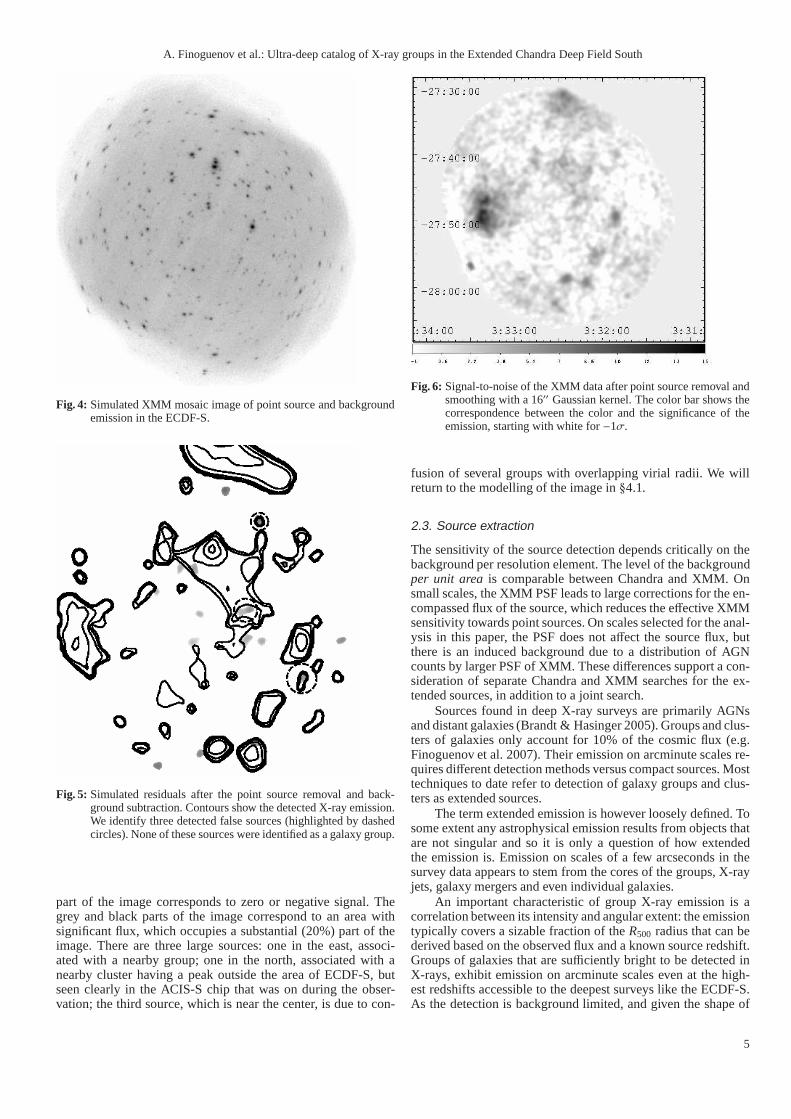
lations of the Lockman Hole (Henry et al. 2010; Brunner et al.2008), finding no residuals. For the ECDF-S, we can extendthose tests to an image a factor of 5 deeper and include the effectsof sub-threshold AGNs down to fluxes of 10−17 ergs s−1 cm−2,based on the deep Chandra catalogs. In Fig.4 we show the simu-lated image and the residuals detected on 32′′ − 128′′ scales. Wehave simulated point sources flux and the background for eachofthe XMM pointings, and followed the procedure for backgroundand point source subtraction.
A total of 16 extended sources have been detected in thesimulated 0.3 square degree mosaic image, while only pointsources were used as an input. These fake extended sourcescorrespond to large-scale distribution of unresolved sources byXMM and each source is made of a combination of typically7 AGNs inside the source and lack of AGNs on either part ofthe source. We also performed a detection of simulated pointsources, adding an error associated with the extra flux due totheextended sources. The number of detected fake sources has notdecreased substantially (15), 8 of those are in the CDF-S area.
Finally, since the positions of the simulated sources are real,they should correspond to an actual extended source in XMM.The number of such detections in XMM mosaic is 3. This is dueto the fact that most of the fake sources being close to the fluxlimit of 2 × 10⁻¹⁶ ergs s−1 cm−2, where detection is affected bythe confusion on extended emission. The 3 detected fake sourceshave a flux of 2, 3, 5×10⁻¹⁶ ergs s−1 cm−2, with a correspond-ing flux error of 1.2 × 10⁻¹⁶ ergs s−1 cm−2, which agrees withthe detected flux by XMM at those positions. None of these fakesources were identified as galaxy groups and entered the finalcatalog. However, they have contributed to a reduction in theidentification rate by 6%. In Fig.5 we overlay the contours ofdetected extended emission over the simulated point sourcecon-tamination image.
In Fig.6 we show the signal-to-noise ratio obtained for thefinal joint dataset (excluding ECDF-S Chandra data) after sub-tracting the background and detected point sources. The white
4
A. Finoguenov et al.: Ultra-deep catalog of X-ray groups in the Extended Chandra Deep Field South
Fig. 4: Simulated XMM mosaic image of point source and backgroundemission in the ECDF-S.
Fig. 5: Simulated residuals after the point source removal and back-ground subtraction. Contours show the detected X-ray emission.We identify three detected false sources (highlighted by dashedcircles). None of these sources were identified as a galaxy group.
part of the image corresponds to zero or negative signal. Thegrey and black parts of the image correspond to an area withsignificant flux, which occupies a substantial (20%) part of theimage. There are three large sources: one in the east, associ-ated with a nearby group; one in the north, associated with anearby cluster having a peak outside the area of ECDF-S, butseen clearly in the ACIS-S chip that was on during the obser-vation; the third source, which is near the center, is due to con-
Fig. 6: Signal-to-noise of the XMM data after point source removal andsmoothing with a 16′′ Gaussian kernel. The color bar shows thecorrespondence between the color and the significance of theemission, starting with white for−1σ.
fusion of several groups with overlapping virial radii. We willreturn to the modelling of the image in§4.1.
2.3. Source extraction
The sensitivity of the source detection depends criticallyon thebackground per resolution element. The level of the backgroundper unit areais comparable between Chandra and XMM. Onsmall scales, the XMM PSF leads to large corrections for the en-compassed flux of the source, which reduces the effective XMMsensitivity towards point sources. On scales selected for the anal-ysis in this paper, the PSF does not affect the source flux, butthere is an induced background due to a distribution of AGNcounts by larger PSF of XMM. These differences support a con-sideration of separate Chandra and XMM searches for the ex-tended sources, in addition to a joint search.
Sources found in deep X-ray surveys are primarily AGNsand distant galaxies (Brandt & Hasinger 2005). Groups and clus-ters of galaxies only account for 10% of the cosmic flux (e.g.Finoguenov et al. 2007). Their emission on arcminute scalesre-quires different detection methods versus compact sources. Mosttechniques to date refer to detection of galaxy groups and clus-ters as extended sources.
The term extended emission is however loosely defined. Tosome extent any astrophysical emission results from objects thatare not singular and so it is only a question of how extendedthe emission is. Emission on scales of a few arcseconds in thesurvey data appears to stem from the cores of the groups, X-rayjets, galaxy mergers and even individual galaxies.
An important characteristic of group X-ray emission is acorrelation between its intensity and angular extent: the emissiontypically covers a sizable fraction of theR500 radius that can bederived based on the observed flux and a known source redshift.Groups of galaxies that are sufficiently bright to be detected inX-rays, exhibit emission on arcminute scales even at the high-est redshifts accessible to the deepest surveys like the ECDF-S.As the detection is background limited, and given the shape of
5
A. Finoguenov et al.: Ultra-deep catalog of X-ray groups in the Extended Chandra Deep Field South
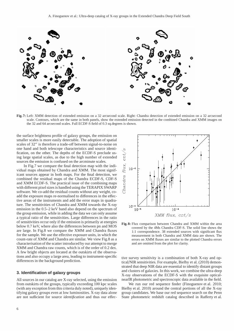
Fig. 7: Left: XMM detection of extended emission on a 32 arcsecond scale. Right: Chandra detection of extended emission on a 32 arcsecondscale. Contours, which are the same in both panels, show the extended emission detected in the combined Chandra and XMM images onthe 32 and 64 arcsecond scales. Full ECDF-S field of 0.3 sq.degrees is shown.
the surface brightness profile of galaxy groups, the emission onsmaller scales is more easily detectable. The adoption of spatialscales of 32′′ is therefore a trade-off between signal-to-noise onone hand and both telescope characteristics and source identi-fication, on the other. The depths of the ECDF-S preclude us-ing large spatial scales, as due to the high number of extendedsources the emission is confused on the arcminute scales.
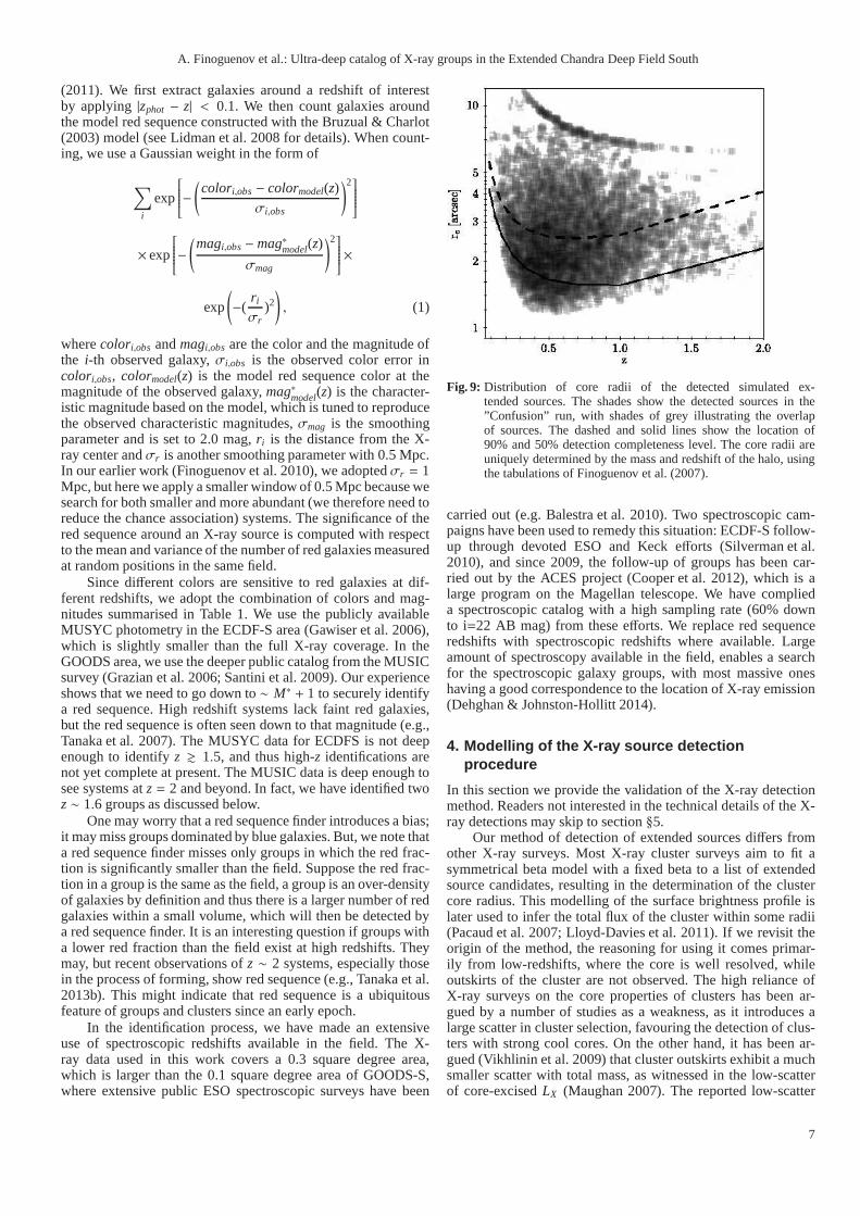
In Fig.7 we compare the final detection map with the indi-vidual maps obtained by Chandra and XMM. The most signif-icant sources appear in both maps. For the final detection, wecombined the residual maps of the Chandra ECDF-S, CDF-Sand XMM ECDF-S. The practical issue of the combining mapswith different pixel sizes is handled using the TERAPIX SWARPsoftware. We co-add the residual counts without any weight,co-add the exposure maps re-normalised to differences in the effec-tive areas of the instruments and add the error maps in quadra-ture. The sensitivities of Chandra and XMM towards the X-rayemission in the 0.5–2 keV band also depend on the spectrum ofthe group emission, while in adding the data we can only assumea typical ratio of the sensitivities. Large differences in the ratioof sensitivities occur only if the emission is primarily at energiesbelow 0.7 keV, where also the differences between pn and MOSare large. In Fig.8 we compare the XMM and Chandra fluxesfor the sample. We use the effective exposure units, in which thecount-rate of XMM and Chandra are similar. We view Fig.8 as acharacterisation of the scatter introduced by our attempt to mergeXMM and Chandra raw counts, which is of the order of 0.2 dex.A few bright objects are located at the outskirts of the observa-tions and also occupy a large area, leading to instrument-specificdifferences in the background prediction.
3. Identification of galaxy groups
All sources in our catalog are X-ray selected, using the emissionfrom outskirts of the groups, typically exceeding 100 kpc scales(with any exception from this criteria duly noted), uniquely iden-tifying galaxy groups even at low luminosities. X-ray data aloneare not sufficient for sourceidentificationand thus our effec-
Fig. 8: Flux comparison between Chandra and XMM within the areacovered by the 4Ms Chandra CDF-S. The solid line shows the1:1 correspondence. 38 extended sources with significant fluxmeasurement in both Chandra and XMM data are shown. Theerrors on XMM fluxes are similar to the plotted Chandra errorsand are omitted from the plot for clarity.
tive survey sensitivity is a combination of both X-ray and op-tical/NIR sensitivities. For example, Bielby et al. (2010) demon-strated that deep NIR data are essential to identify distantgroupsand clusters of galaxies. In this work, we combine the ultra-deepX-ray observations of the ECDF-S with the exquisite optical-nearIR photometric and spectroscopic data available in thefield.
We run our red sequence finder (Finoguenov et al. 2010;Bielby et al. 2010) around the central portions of all the X-raygroup candidates. We base our red sequence search on the PennState photometric redshift catalog described in Rafferty et al.
6
A. Finoguenov et al.: Ultra-deep catalog of X-ray groups in the Extended Chandra Deep Field South
(2011). We first extract galaxies around a redshift of interestby applying |zphot − z| < 0.1. We then count galaxies aroundthe model red sequence constructed with the Bruzual & Charlot(2003) model (see Lidman et al. 2008 for details). When count-ing, we use a Gaussian weight in the form of
∑
i
exp
−
(
colori,obs− colormodel(z)σi,obs
)2
× exp
−
(
magi,obs−mag∗model(z)
σmag
)2
×
exp
(
−(r i
σr)2
)
, (1)
wherecolori,obs andmagi,obs are the color and the magnitude ofthe i-th observed galaxy,σi,obs is the observed color error incolori,obs, colormodel(z) is the model red sequence color at themagnitude of the observed galaxy,mag∗model(z) is the character-istic magnitude based on the model, which is tuned to reproducethe observed characteristic magnitudes,σmag is the smoothingparameter and is set to 2.0 mag,r i is the distance from the X-ray center andσr is another smoothing parameter with 0.5 Mpc.In our earlier work (Finoguenov et al. 2010), we adoptedσr = 1Mpc, but here we apply a smaller window of 0.5 Mpc because wesearch for both smaller and more abundant (we therefore needtoreduce the chance association) systems. The significance ofthered sequence around an X-ray source is computed with respectto the mean and variance of the number of red galaxies measuredat random positions in the same field.
Since different colors are sensitive to red galaxies at dif-ferent redshifts, we adopt the combination of colors and mag-nitudes summarised in Table 1. We use the publicly availableMUSYC photometry in the ECDF-S area (Gawiser et al. 2006),which is slightly smaller than the full X-ray coverage. In theGOODS area, we use the deeper public catalog from the MUSICsurvey (Grazian et al. 2006; Santini et al. 2009). Our experienceshows that we need to go down to∼ M∗ + 1 to securely identifya red sequence. High redshift systems lack faint red galaxies,but the red sequence is often seen down to that magnitude (e.g.,Tanaka et al. 2007). The MUSYC data for ECDFS is not deepenough to identifyz & 1.5, and thus high-z identifications arenot yet complete at present. The MUSIC data is deep enough tosee systems atz= 2 and beyond. In fact, we have identified twoz∼ 1.6 groups as discussed below.
One may worry that a red sequence finder introduces a bias;it may miss groups dominated by blue galaxies. But, we note thata red sequence finder misses only groups in which the red frac-tion is significantly smaller than the field. Suppose the red frac-tion in a group is the same as the field, a group is an over-densityof galaxies by definition and thus there is a larger number of redgalaxies within a small volume, which will then be detected bya red sequence finder. It is an interesting question if groupswitha lower red fraction than the field exist at high redshifts. Theymay, but recent observations ofz ∼ 2 systems, especially thosein the process of forming, show red sequence (e.g., Tanaka etal.2013b). This might indicate that red sequence is a ubiquitousfeature of groups and clusters since an early epoch.
In the identification process, we have made an extensiveuse of spectroscopic redshifts available in the field. The X-ray data used in this work covers a 0.3 square degree area,which is larger than the 0.1 square degree area of GOODS-S,where extensive public ESO spectroscopic surveys have been
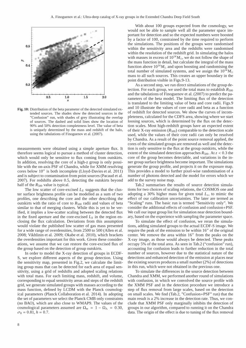
Fig. 9: Distribution of core radii of the detected simulated ex-tended sources. The shades show the detected sources in the”Confusion” run, with shades of grey illustrating the overlapof sources. The dashed and solid lines show the location of90% and 50% detection completeness level. The core radii areuniquely determined by the mass and redshift of the halo, usingthe tabulations of Finoguenov et al. (2007).
carried out (e.g. Balestra et al. 2010). Two spectroscopic cam-paigns have been used to remedy this situation: ECDF-S follow-up through devoted ESO and Keck efforts (Silverman et al.2010), and since 2009, the follow-up of groups has been car-ried out by the ACES project (Cooper et al. 2012), which is alarge program on the Magellan telescope. We have complieda spectroscopic catalog with a high sampling rate (60% downto i=22 AB mag) from these efforts. We replace red sequenceredshifts with spectroscopic redshifts where available. Largeamount of spectroscopy available in the field, enables a searchfor the spectroscopic galaxy groups, with most massive oneshaving a good correspondence to the location of X-ray emission(Dehghan & Johnston-Hollitt 2014).
4. Modelling of the X-ray source detectionprocedure
In this section we provide the validation of the X-ray detectionmethod. Readers not interested in the technical details of the X-ray detections may skip to section§5.
Our method of detection of extended sources differs fromother X-ray surveys. Most X-ray cluster surveys aim to fit asymmetrical beta model with a fixed beta to a list of extendedsource candidates, resulting in the determination of the clustercore radius. This modelling of the surface brightness profile islater used to infer the total flux of the cluster within some radii(Pacaud et al. 2007; Lloyd-Davies et al. 2011). If we revisittheorigin of the method, the reasoning for using it comes primar-ily from low-redshifts, where the core is well resolved, whileoutskirts of the cluster are not observed. The high relianceofX-ray surveys on the core properties of clusters has been ar-gued by a number of studies as a weakness, as it introduces alarge scatter in cluster selection, favouring the detection of clus-ters with strong cool cores. On the other hand, it has been ar-gued (Vikhlinin et al. 2009) that cluster outskirts exhibita muchsmaller scatter with total mass, as witnessed in the low-scatterof core-excisedLX (Maughan 2007). The reported low-scatter
7
A. Finoguenov et al.: Ultra-deep catalog of X-ray groups in the Extended Chandra Deep Field South
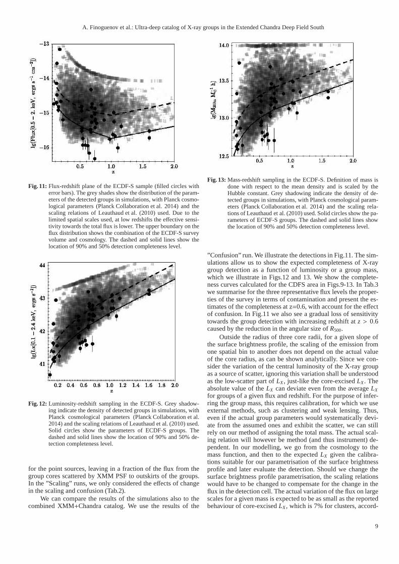
Fig. 10: Distribution of the beta parameter of the detected simulated ex-tended sources. The shades show the detected sources in the”Confusion” run, with shades of grey illustrating the overlapof sources. The dashed and solid lines show the location of90% and 50% detection completeness level. The value of betais uniquely determined by the mass and redshift of the halo,using the tabulations of Finoguenov et al. (2007).
measurements were obtained using a simple aperture flux. Ittherefore seems logical to pursue a method of cluster detection,which would only be sensitive to flux coming from outskirts.In addition, resolving the core of a high-z group is only possi-ble with the on-axis PSF of Chandra, while for XMM resolvingcores below 10′′ is both incomplete (Lloyd-Davies et al. 2011)and is subject to contamination from point sources (Pacaud et al.2007). For redshifts above 0.5, detecting the outskirts beyondhalf of theR500 value is typical.
The low scatter of core-excisedLX suggests that the clus-ter surface brightness profile can be modelled as a sum of twoprofiles, one describing the core and the other describing theoutskirts with the ratio of core toR500 radii and values of betasimilar to that of merging clusters. While this is yet to be ver-ified, it implies a low-scatter scaling between the detectedfluxin the fixed aperture and the core-excisedLX in the region en-closing the flux calculation. Deviations from this assumptionwould violate the published low scatter of gas mass presentedfor a wide range of overdensities, from 2500 to 500 (Allen et al.2008; Vikhlinin et al. 2009; Okabe et al. 2010), which bracketsthe overdensities important for this work. Given these consider-ations, we assume that we can restore the core-excised flux ofthe group based on the detection of group outskirts.
In order to model the X-ray detection of groups in ECDF-S, we explore different aspects of the group detection. Usingthe sensitivity map, presented in Fig.2, we calculate the limit-ing group mass that can be detected for each area of equal sen-sitivity, using a grid of redshifts and adopted scaling relationswith total mass. For each limiting mass, redshift, and volume,corresponding to equal sensitivity areas and steps of the redshiftgrid, we generate simulated groups with masses according tothemass function, defined by LCDM with the Planck cosmolog-ical parameters (Planck Collaboration et al. 2014). In adoptingthe set of parameters we select the Planck CMB only constraints(no BAO), which are also close to WMAP9. The values of thecosmological parameters assumed areΩm = 1 − ΩΛ = 0.30,σ8 = 0.81,h = 0.7.
With about 100 groups expected from the cosmology, wewould not be able to sample well all the parameter space im-portant for detection and so the expected numbers were boostedby a factor of 100, constrained by the time required to performthe simulations. The positions of the groups were randomisedwithin the sensitivity area and the redshifts were randomisedwithin the resolution of the redshift grid. In simulating the haloswith masses in excess of 1014M⊙, we do not follow the shape ofthe mass function in detail, but calculate the integral of the massfunction above 1014M⊙ and upon boosting and randomising thetotal number of simulated systems, and we assign the 1014M⊙mass to all such sources. This creates an upper boundary in thepoint distribution visible in Figs.9-13.
As a second step, we run direct simulations of the group de-tection. For each group, we used the total mass to establishR500and the tabulations of Finoguenov et al. (2007) to predict the pa-rameters of the beta model. The limiting flux of the detectionis translated to the limiting value of beta and core radii. Figs.9and 10 illustrate the values of core radii and beta as a functionof redshift for detected sources. We show the curves of incom-pleteness, calculated for the CDFS area, showing where we startloosing sources, which is determined by the flux on the detec-tion scales. Most high-redshift groups have an expected extentof their X-ray emission (R500) comparable to the detection scaleused, while the values of their core radii can only be resolvedby Chandra. As a result of the point source removal applied, thecores of the simulated groups are removed as well and the detec-tion is only sensitive to the flux at the group outskirts, while theextent of the simulated detection approachesR500. At z< 0.3 thecore of the group becomes detectable, and variations in the in-ner group surface brightness become important. The simulationsgenerate the group profile, and projects it on the exposure map.This provides a model to further pixel-wise randomisation of anumber of photons detected and the model for errors which weadd to the survey noise map.
Tab.2 summarises the results of source detection simula-tions for two choices of scaling relations, the COSMOS one andadopting a 30% higher mass for given totalLx, to mimic theeffect of our calibration uncertainties. The later are termed as”Scaling” runs. The basic run is termed ”Sensitivity only”.Weconsider the additional effects of confusion and confusion+PSF.We cull our input group list for simulation near detection bound-ary, based on the experience with sampling the parameter space.
To simulate the effect of confusion, we reran the simula-tions, adding simulated groups to the actual ECDF-S image. Werequire the peak of the emission to be within 16′′ of the originalcenter. We remove the area within 16′′ from the peaks on theX-ray image, as those would always be detected. These peaksoccupy 5% of the total area. As seen in Tab.2 (“confusion” run),accounting for confusion leads to further reduction in the totalnumber of sources, however due to the statistical nature of thedetections and enhanced detection of the emission at placesnearthe existing sources produces a small number (2%) of detectionsin this run, which were not obtained in the previous one.
To simulate the differences in the source detection betweenChandra and XMM, we performed another round of simulationswith confusion, in which we convolved the source profile withthe XMM PSF and in the detection procedure we introduce astep of flux removal from large scales, based on the detectionon small scales. We find (Tab.2, ”Confusion+PSF” run) that themain result is a 2% increase in the detection rate. Thus, we con-clude that XMM PSF only marginally inhibits the detection ofgroups in our algorithm, compared to running it on the Chandradata. The origin of the effect is due to tuning of the flux removal
8
A. Finoguenov et al.: Ultra-deep catalog of X-ray groups in the Extended Chandra Deep Field South
Fig. 11: Flux-redshift plane of the ECDF-S sample (filled circles witherror bars). The grey shades show the distribution of the param-eters of the detected groups in simulations, with Planck cosmo-logical parameters (Planck Collaboration et al. 2014) and thescaling relations of Leauthaud et al. (2010) used. Due to thelimited spatial scales used, at low redshifts the effective sensi-tivity towards the total flux is lower. The upper boundary on theflux distribution shows the combination of the ECDF-S surveyvolume and cosmology. The dashed and solid lines show thelocation of 90% and 50% detection completeness level.
Fig. 12: Luminosity-redshift sampling in the ECDF-S. Grey shadow-ing indicate the density of detected groups in simulations,withPlanck cosmological parameters (Planck Collaboration et al.2014) and the scaling relations of Leauthaud et al. (2010) used.Solid circles show the parameters of ECDF-S groups. Thedashed and solid lines show the location of 90% and 50% de-tection completeness level.
for the point sources, leaving in a fraction of the flux from thegroup cores scattered by XMM PSF to outskirts of the groups.In the ”Scaling” runs, we only considered the effects of changein the scaling and confusion (Tab.2).
We can compare the results of the simulations also to thecombined XMM+Chandra catalog. We use the results of the
Fig. 13: Mass-redshift sampling in the ECDF-S. Definition of mass isdone with respect to the mean density and is scaled by theHubble constant. Grey shadowing indicate the density of de-tected groups in simulations, with Planck cosmological param-eters (Planck Collaboration et al. 2014) and the scaling rela-tions of Leauthaud et al. (2010) used. Solid circles show thepa-rameters of ECDF-S groups. The dashed and solid lines showthe location of 90% and 50% detection completeness level.
”Confusion” run. We illustrate the detections in Fig.11. The sim-ulations allow us to show the expected completeness of X-raygroup detection as a function of luminosity or a group mass,which we illustrate in Figs.12 and 13. We show the complete-ness curves calculated for the CDFS area in Figs.9-13. In Tab.3we summarise for the three representative flux levels the proper-ties of the survey in terms of contamination and present the es-timates of the completeness at z=0.6, with account for the effectof confusion. In Fig.11 we also see a gradual loss of sensitivitytowards the group detection with increasing redshift atz > 0.6caused by the reduction in the angular size ofR500.
Outside the radius of three core radii, for a given slope ofthe surface brightness profile, the scaling of the emission fromone spatial bin to another does not depend on the actual valueof the core radius, as can be shown analytically. Since we con-sider the variation of the central luminosity of the X-ray groupas a source of scatter, ignoring this variation shall be understoodas the low-scatter part ofLX, just-like the core-excisedLX. Theabsolute value of theLX can deviate even from the averageLXfor groups of a given flux and redshift. For the purpose of infer-ring the group mass, this requires calibration, for which weuseexternal methods, such as clustering and weak lensing. Thus,even if the actual group parameters would systematically devi-ate from the assumed ones and exhibit the scatter, we can stillrely on our method of assigning the total mass. The actual scal-ing relation will however be method (and thus instrument) de-pendent. In our modelling, we go from the cosmology to themass function, and then to the expectedLX given the calibra-tions suitable for our parametrisation of the surface brightnessprofile and later evaluate the detection. Should we change thesurface brightness profile parametrisation, the scaling relationswould have to be changed to compensate for the change in theflux in the detection cell. The actual variation of the flux on largescales for a given mass is expected to be as small as the reportedbehaviour of core-excisedLX, which is 7% for clusters, accord-
9
A. Finoguenov et al.: Ultra-deep catalog of X-ray groups in the Extended Chandra Deep Field South
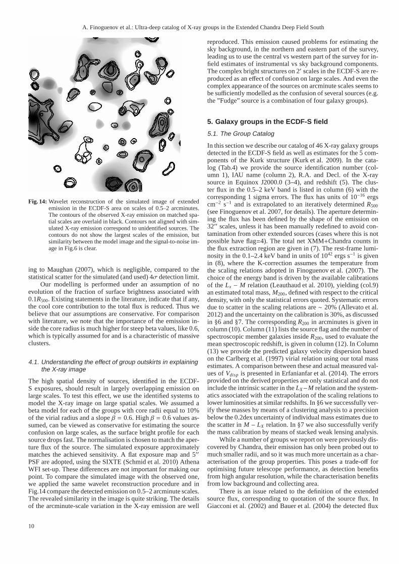
Fig. 14: Wavelet reconstruction of the simulated image of extendedemission in the ECDF-S area on scales of 0.5–2 arcminutes.The contours of the observed X-ray emission on matched spa-tial scales are overlaid in black. Contours not aligned withsim-ulated X-ray emission correspond to unidentified sources. Thecontours do not show the largest scales of the emission, butsimilarity between the model image and the signal-to-noiseim-age in Fig.6 is clear.
ing to Maughan (2007), which is negligible, compared to thestatistical scatter for the simulated (and used) 4σ detection limit.
Our modelling is performed under an assumption of noevolution of the fraction of surface brightness associatedwith0.1R500. Existing statements in the literature, indicate that if any,the cool core contribution to the total flux is reduced. Thus webelieve that our assumptions are conservative. For comparisonwith literature, we note that the importance of the emissionin-side the core radius is much higher for steep beta values, like 0.6,which is typically assumed for and is a characteristic of massiveclusters.
4.1. Understanding the effect of group outskirts in explainingthe X-ray image
The high spatial density of sources, identified in the ECDF-S exposures, should result in largely overlapping emissiononlarge scales. To test this effect, we use the identified systems tomodel the X-ray image on large spatial scales. We assumed abeta model for each of the groups with core radii equal to 10%of the virial radius and a slopeβ = 0.6. Highβ = 0.6 values as-sumed, can be viewed as conservative for estimating the sourceconfusion on large scales, as the surface bright profile for eachsource drops fast. The normalisation is chosen to match the aper-ture flux of the source. The simulated exposure approximatelymatches the achieved sensitivity. A flat exposure map and 5′′
PSF are adopted, using the SIXTE (Schmid et al. 2010) AthenaWFI set-up. These differences are not important for making ourpoint. To compare the simulated image with the observed one,we applied the same wavelet reconstruction procedure and inFig.14 compare the detected emission on 0.5–2 arcminute scales.The revealed similarity in the image is quite striking. The detailsof the arcminute-scale variation in the X-ray emission are well
reproduced. This emission caused problems for estimating thesky background, in the northern and eastern part of the survey,leading us to use the central vs western part of the survey forin-field estimates of instrumental vs sky background components.The complex bright structures on 2′ scales in the ECDF-S are re-produced as an effect of confusion on large scales. And even thecomplex appearance of the sources on arcminute scales seemstobe sufficiently modelled as the confusion of several sources (e.g.the ”Fudge” source is a combination of four galaxy groups).
5. Galaxy groups in the ECDF-S field
5.1. The Group Catalog
In this section we describe our catalog of 46 X-ray galaxy groupsdetected in the ECDF-S field as well as estimates for the 5 com-ponents of the Kurk structure (Kurk et al. 2009). In the cata-log (Tab.4) we provide the source identification number (col-umn 1), IAU name (column 2), R.A. and Decl. of the X-raysource in Equinox J2000.0 (3–4), and redshift (5). The clus-ter flux in the 0.5–2 keV band is listed in column (6) with thecorresponding 1 sigma errors. The flux has units of 10−16 ergscm−2 s−1 and is extrapolated to an iteratively determinedR500(see Finoguenov et al. 2007, for details). The aperture determin-ing the flux has been defined by the shape of the emission on32′′ scales, unless it has been manually redefined to avoid con-tamination from other extended sources (cases where this isnotpossible have flag=4). The total net XMM+Chandra counts inthe flux extraction region are given in (7). The rest-frame lumi-nosity in the 0.1–2.4 keV band in units of 1042 ergs s−1 is givenin (8), where the K-correction assumes the temperature fromthe scaling relations adopted in Finoguenov et al. (2007). Thechoice of the energy band is driven by the available calibrationsof the Lx − M relation (Leauthaud et al. 2010), yielding (col.9)an estimated total mass,M200, defined with respect to the criticaldensity, with only the statistical errors quoted. Systematic errorsdue to scatter in the scaling relations are∼ 20% (Allevato et al.2012) and the uncertainty on the calibration is 30%, as discussedin §6 and§7. The correspondingR200 in arcminutes is given incolumn (10). Column (11) lists the source flag and the number ofspectroscopic member galaxies insideR200, used to evaluate themean spectroscopic redshift, is given in column (12). In Column(13) we provide the predicted galaxy velocity dispersion basedon the Carlberg et al. (1997) virial relation using our totalmassestimates. A comparison between these and actual measured val-ues ofVdisp is presented in Erfanianfar et al. (2014). The errorsprovided on the derived properties are only statistical anddo notinclude the intrinsic scatter in theLX−M relation and the system-atics associated with the extrapolation of the scaling relations tolower luminosities at similar redshifts. In§6 we successfully ver-ify these masses by means of a clustering analysis to a precisionbelow the 0.2dex uncertainty of individual mass estimates due tothe scatter inM − LX relation. In§7 we also successfully verifythe mass calibration by means of stacked weak lensing analysis.
While a number of groups we report on were previously dis-covered by Chandra, their emission has only been probed out tomuch smaller radii, and so it was much more uncertain as a char-acterisation of the group properties. This poses a trade-off foroptimising future telescope performance, as detection benefitsfrom high angular resolution, while the characterisation benefitsfrom low background and collecting area.
There is an issue related to the definition of the extendedsource flux, corresponding to quotation of the source flux. InGiacconi et al. (2002) and Bauer et al. (2004) the detected flux
10
A. Finoguenov et al.: Ultra-deep catalog of X-ray groups in the Extended Chandra Deep Field South
is quoted, while in Finoguenov et al. (2007, 2010) the full fluxof the source is quoted. These can be different by a factor of afew. Using the large spatial scales, one reduces the amount ofextrapolation on the flux and therefore removes a large separa-tion between the observed and referred flux, which is subjecttomodel assumptions (Connelly et al. 2012).
In Finoguenov et al. (2007, 2010); Bielby et al. (2010) weintroduced a system of flagging the source identification. The ob-jects with flag=1 are of best quality, with centroids derived fromthe X-ray emission and spectroscopic confirmation of the red-shift; flag=2 objects have large uncertainties in the X-ray center(low statistics or source confusion) with their centroids and fluxextraction apertures positioned on the associated galaxy concen-tration with spectroscopic confirmation; objects with flag=3 stillrequire spectroscopic confirmation; objects with flag=4 havemore than one counterpart along the line of sight; objects withflag=5 have doubtful identifications and are only used to accesssystematic errors in the statistical analysis associated with sourceidentification.
Using a catalog of Miller et al. (2013) we find a number ofcomplex radio sources inside the X-ray galaxy groups, the cor-respondent group ids are: 3, 12, 19 (contains a Wide AngularTail source), 26, 43, 52, 57. All these sources do not have a two-dimensional match of the shape of their X-ray emission with theradio. In all cases, but group 43, we can also rule out a substantial(> 10%) contribution of the IC emission associated with radiosource to the X-ray flux. For group 43 this contribution can beup to 50%, estimated using the part of the source flux in the areaoverlapping with the radio emission. We note that the associatedwith group 43 radio galaxy is the strongest FRII source in CDFS.Other studies typically find one IC X-ray source per square de-gree (Jelic et al. 2012), so the statistics of CDFS is consistentwith that.
5.2. Statistical properties of the groups
In Fig.11 we plot the sample in the flux-redshift plane. The con-fusion of sources and our approach to reduce it using 32′′ spatialscales for the flux extraction, results in large flux corrections atlow-z. The correction approaches unity (thus no correctionatall) for z > 0.5 sources with a high significance of the detec-tion. This also introduces a redshift dependence to the flux limit,with a limiting flux of 10−15 ergs s−1 cm−2 at z=0.05 levellingoff at 1.5 × 10⁻¹⁶ ergs s−1 cm−2 at the redshifts exceeding 0.5.However, to account for this effect is straight-forward. Our ex-perience shows that different science goals require different sub-samples, a mass-limited sample, for example, would be selecteddifferently. Also, some definition of galaxy groups would makea cut on X-ray luminosity, removing the need for an equal flux.For most of our own work, the high-z galaxy groups are the onesthat we are most interested in (Ziparo et al. 2013, 2014).
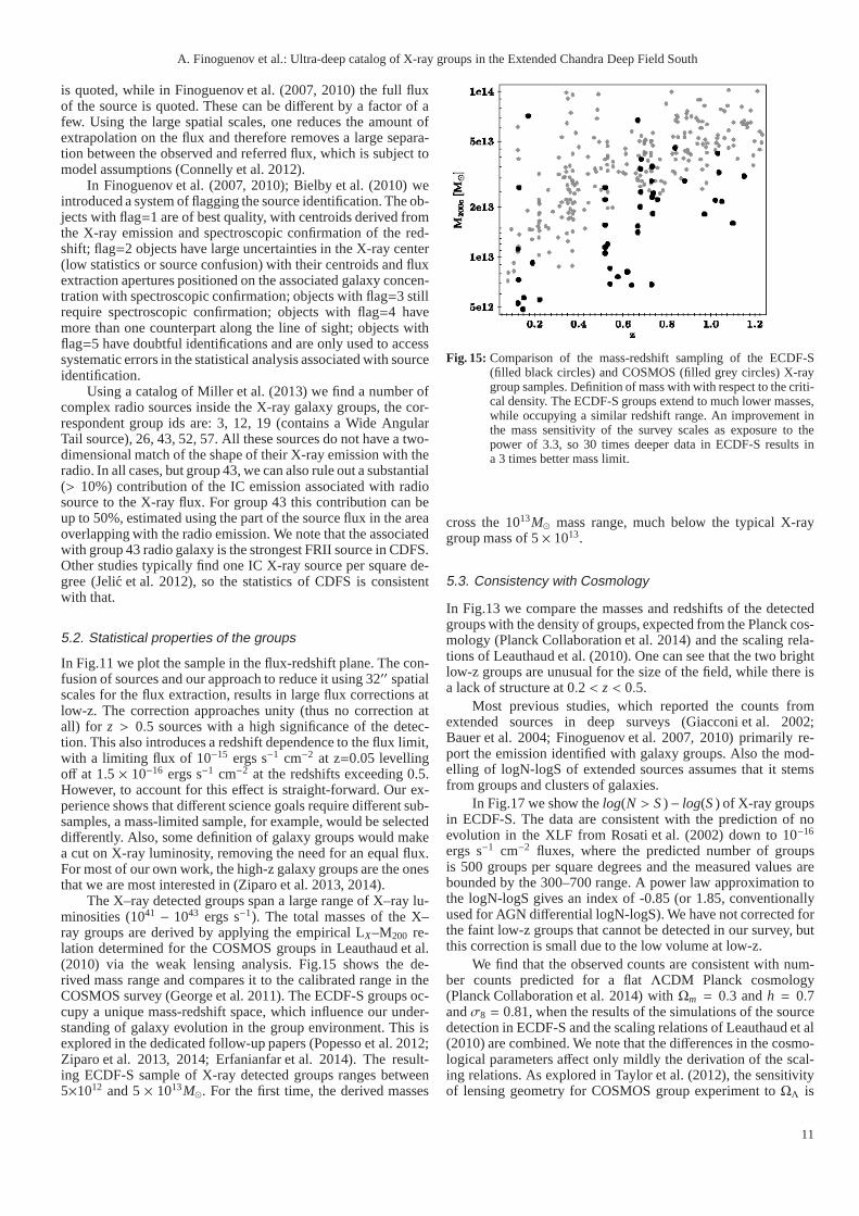
The X–ray detected groups span a large range of X–ray lu-minosities (1041 − 1043 ergs s−1). The total masses of the X–ray groups are derived by applying the empirical LX–M200 re-lation determined for the COSMOS groups in Leauthaud et al.(2010) via the weak lensing analysis. Fig.15 shows the de-rived mass range and compares it to the calibrated range in theCOSMOS survey (George et al. 2011). The ECDF-S groups oc-cupy a unique mass-redshift space, which influence our under-standing of galaxy evolution in the group environment. Thisisexplored in the dedicated follow-up papers (Popesso et al. 2012;Ziparo et al. 2013, 2014; Erfanianfar et al. 2014). The result-ing ECDF-S sample of X-ray detected groups ranges between5×1012 and 5× 10¹³M⊙. For the first time, the derived masses
Fig. 15: Comparison of the mass-redshift sampling of the ECDF-S(filled black circles) and COSMOS (filled grey circles) X-raygroup samples. Definition of mass with with respect to the criti-cal density. The ECDF-S groups extend to much lower masses,while occupying a similar redshift range. An improvement inthe mass sensitivity of the survey scales as exposure to thepower of 3.3, so 30 times deeper data in ECDF-S results ina 3 times better mass limit.
cross the 1013M⊙ mass range, much below the typical X-raygroup mass of 5× 10¹³.
5.3. Consistency with Cosmology
In Fig.13 we compare the masses and redshifts of the detectedgroups with the density of groups, expected from the Planck cos-mology (Planck Collaboration et al. 2014) and the scaling rela-tions of Leauthaud et al. (2010). One can see that the two brightlow-z groups are unusual for the size of the field, while thereisa lack of structure at 0.2 < z< 0.5.
Most previous studies, which reported the counts fromextended sources in deep surveys (Giacconi et al. 2002;Bauer et al. 2004; Finoguenov et al. 2007, 2010) primarily re-port the emission identified with galaxy groups. Also the mod-elling of logN-logS of extended sources assumes that it stemsfrom groups and clusters of galaxies.
In Fig.17 we show thelog(N > S)− log(S) of X-ray groupsin ECDF-S. The data are consistent with the prediction of noevolution in the XLF from Rosati et al. (2002) down to 10−16
ergs s−1 cm−2 fluxes, where the predicted number of groupsis 500 groups per square degrees and the measured values arebounded by the 300–700 range. A power law approximation tothe logN-logS gives an index of -0.85 (or 1.85, conventionallyused for AGN differential logN-logS). We have not corrected forthe faint low-z groups that cannot be detected in our survey,butthis correction is small due to the low volume at low-z.
We find that the observed counts are consistent with num-ber counts predicted for a flatΛCDM Planck cosmology(Planck Collaboration et al. 2014) withΩm = 0.3 andh = 0.7andσ8 = 0.81, when the results of the simulations of the sourcedetection in ECDF-S and the scaling relations of Leauthaud et al(2010) are combined. We note that the differences in the cosmo-logical parameters affect only mildly the derivation of the scal-ing relations. As explored in Taylor et al. (2012), the sensitivityof lensing geometry for COSMOS group experiment toΩΛ is
11
A. Finoguenov et al.: Ultra-deep catalog of X-ray groups in the Extended Chandra Deep Field South
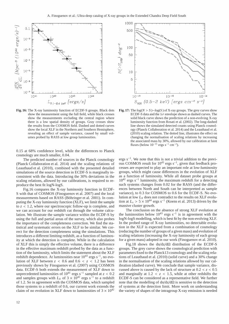
Fig. 16: The X-ray luminosity function of ECDF-S groups. Black dotsshow the measurement using the full field, while black crossesshow the measurements excluding the central region wherethere is a low spatial density of groups. Gray crosses showthe results from the COSMOS field. Dashed and dotted curvesshow the local XLF in the Northern and Southern Hemisphere,revealing an effect of sample variance, caused by small vol-umes probed by RASS at low group luminosities.
0.15 at 68% confidence level, while the differences to Planckcosmology are much smaller, 0.04.
The predicted number of sources in the Planck cosmology(Planck Collaboration et al. 2014) and the scaling relations ofLeauthaud et al. (2010), combined with the presented detailedsimulations of the source detection in ECDF-S is marginallyin-consistent with the data. Introducing the 30% deviations inthescaling relations, allowed by our calibrations, is required to re-produce the best fit logN-logS.
Fig.16 compares the X-ray luminosity function in ECDF-S with that of COSMOS (Finoguenov et al. 2007) and the localmeasurements based on RASS (Bohringer et al. 2001). In com-puting the X-ray luminosity function (XLF), we limit the sampleto z < 1.2, where our spectroscopic follow-up is complete, andwe can account for our redshift cut through the volume calcu-lation. We illustrate the sample variance within the ECDF-Sbyusing the full and partial areas of the survey, which also probesthe importance of the completeness correction. We find the sta-tistical and systematic errors on the XLF to be similar. We cor-rect for the detection completeness using the simulations.Thisintroduces a different limiting redshift, as a function of luminos-ity at which the detection is complete. While in the calculationof XLF this is simply the effective volume, there is a differencein the effective maximum redshift probed by the data as a func-tion of the luminosity, which limits the statement about theXLFredshift dependence. At luminosities near 1043 ergs s−1, no evo-lution of XLF betweenz < 0.6 and 0.6 < z < 1.2 has beenpreviously shown by Finoguenov et al. (2007) using COSMOSdata. ECDF-S both extends the measurement of XLF down tounprecedented luminosities of 1041 ergs s−1 sampled atz < 0.2and samples groups withLX of 3 × 1042 ergs s−1 to a redshiftof 1.2. So in agreement with the COSMOS data, which sampledthose systems to a redshift of 0.6, our current work extends theclaim of no evolution in XLF down to luminosities of 3× 1042
Fig. 17: Thelog(N > S)−log(S) of X-ray groups. The grey curves showECDF-S data and the 1σ envelope shown as dashed curves. Thesolid black curve shows the prediction of a non-evolving X-rayluminosity function from Rosati et al. (2002). The long-dashedline shows the simulated detected counts using Planck cosmol-ogy (Planck Collaboration et al. 2014) and the Leauthaud et al.(2010) scaling relation. The dotted line, illustrates the effect onchanging the normalisation of scaling relations by increasingthe associated mass by 30%, allowed by our calibration at faintfluxes (below 10−15 ergs s−1 cm−2).
ergs s−1. We note that this is not a trivial addition to the previ-ous COSMOS result for 1043 ergs s−1, given that feedback pro-cesses are expected to play an important role at low-luminositygroups, which might cause differences in the evolution of XLFas a function of luminosity. While all dataset probe groups at1042 ergs s−1 luminosity, the maximum redshift for a detectingsuch systems changes from 0.02 for the RASS (and the differ-ences between North and South can be interpretted as samplevariance), to 0.3 for COSMOS to 0.6 for the ECDF-S. No evo-lution at lowLX does not contradict to the results on XLF evolu-tion at Lx > 5× 1044 ergs s−1 (Koens et al. 2013) driven by themassive cluster growth.
The conclusion on the absence of strong XLF evolution atthe luminosities below 1043 ergs s−1 is in agreement with thelogN-logS modelling, which is best fit by the non-evolving XLF.In the probed range of X-ray luminosities, no detectable evolu-tion in the XLF is expected from a combination of cosmology(reducing the number of groups of a given mass) and evolutionofscaling relations (increasing the X-ray luminosity of eachgroupfor a given mass) adopted in our work (Finoguenov et al. 2010).
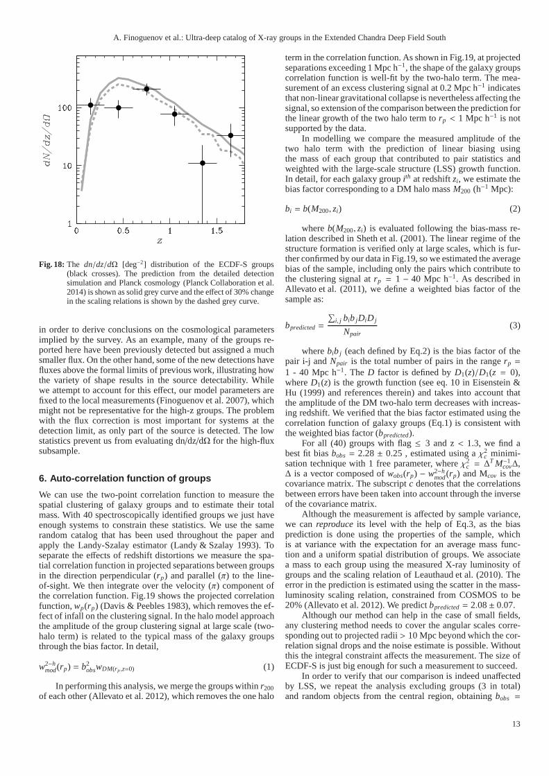
Fig.18 shows the dn/dz/dΩ distribution of the ECDF-Sgroups. The grey curve shows the cosmological prediction withparameters fixed to the Planck13 cosmology and the scaling rela-tions of Leauthaud et al. (2010) (solid curve) and a 30% changein the normalisation of the scaling relations allowed by ourcal-ibration (dashed curve). We conclude that sample variance,dis-cussed above is caused by the lack of structure at 0.2 < z < 0.5and marginally at 1.2 < z < 1.5, while at other redshifts theECDF-S can be considered as a representative field. We furthernote that the modelling of dn/dz/dΩ is sensitive to the detectionof systems at the detection limit. More work on understandingthe variety of shapes of the intragroup X-ray emission is needed
12
A. Finoguenov et al.: Ultra-deep catalog of X-ray groups in the Extended Chandra Deep Field South
Fig. 18: The dn/dz/dΩ [deg−2] distribution of the ECDF-S groups(black crosses). The prediction from the detailed detectionsimulation and Planck cosmology (Planck Collaboration et al.2014) is shown as solid grey curve and the effect of 30% changein the scaling relations is shown by the dashed grey curve.
in order to derive conclusions on the cosmological parametersimplied by the survey. As an example, many of the groups re-ported here have been previously detected but assigned a muchsmaller flux. On the other hand, some of the new detections havefluxes above the formal limits of previous work, illustrating howthe variety of shape results in the source detectability. Whilewe attempt to account for this effect, our model parameters arefixed to the local measurements (Finoguenov et al. 2007), whichmight not be representative for the high-z groups. The problemwith the flux correction is most important for systems at thedetection limit, as only part of the source is detected. The lowstatistics prevent us from evaluating dn/dz/dΩ for the high-fluxsubsample.
6. Auto-correlation function of groups
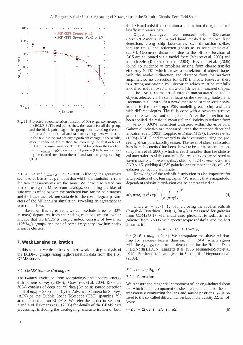
We can use the two-point correlation function to measure thespatial clustering of galaxy groups and to estimate their totalmass. With 40 spectroscopically identified groups we just haveenough systems to constrain these statistics. We use the samerandom catalog that has been used throughout the paper andapply the Landy-Szalay estimator (Landy & Szalay 1993). Toseparate the effects of redshift distortions we measure the spa-tial correlation function in projected separations between groupsin the direction perpendicular (rp) and parallel (π) to the line-of-sight. We then integrate over the velocity (π) component ofthe correlation function. Fig.19 shows the projected correlationfunction,wp(rp) (Davis & Peebles 1983), which removes the ef-fect of infall on the clustering signal. In the halo model approachthe amplitude of the group clustering signal at large scale (two-halo term) is related to the typical mass of the galaxy groupsthrough the bias factor. In detail,
w2−hmod(rp) = b2
obswDM(rp,z=0) (1)
In performing this analysis, we merge the groups withinr200of each other (Allevato et al. 2012), which removes the one halo
term in the correlation function. As shown in Fig.19, at projectedseparations exceeding 1 Mpc h−1, the shape of the galaxy groupscorrelation function is well-fit by the two-halo term. The mea-surement of an excess clustering signal at 0.2 Mpc h−1 indicatesthat non-linear gravitational collapse is nevertheless affecting thesignal, so extension of the comparison between the prediction forthe linear growth of the two halo term torp < 1 Mpc h−1 is notsupported by the data.
In modelling we compare the measured amplitude of thetwo halo term with the prediction of linear biasing usingthe mass of each group that contributed to pair statistics andweighted with the large-scale structure (LSS) growth function.In detail, for each galaxy groupith at redshiftzi , we estimate thebias factor corresponding to a DM halo massM200 (h−1 Mpc):
bi = b(M200, zi) (2)
whereb(M200, zi) is evaluated following the bias-mass re-lation described in Sheth et al. (2001). The linear regime ofthestructure formation is verified only at large scales, which is fur-ther confirmed by our data in Fig.19, so we estimated the averagebias of the sample, including only the pairs which contribute tothe clustering signal atrp = 1 − 40 Mpc h−1. As described inAllevato et al. (2011), we define a weighted bias factor of thesample as:
bpredicted=
∑
i, j bib jDiD j
Npair(3)
wherebib j (each defined by Eq.2) is the bias factor of thepair i-j andNpair is the total number of pairs in the rangerp =
1 - 40 Mpc h−1. The D factor is defined byD1(z)/D1(z = 0),whereD1(z) is the growth function (see eq. 10 in Eisenstein &Hu (1999) and references therein) and takes into account thatthe amplitude of the DM two-halo term decreases with increas-ing redshift. We verified that the bias factor estimated using thecorrelation function of galaxy groups (Eq.1) is consistentwiththe weighted bias factor (bpredicted).
For all (40) groups with flag≤ 3 and z< 1.3, we find abest fit biasbobs = 2.28± 0.25 , estimated using aχ2
c minimi-sation technique with 1 free parameter, whereχ2
c = ∆T M−1
cov∆,∆ is a vector composed ofwobs(rp) − w2−h
mod(rp) and Mcov is thecovariance matrix. The subscriptc denotes that the correlationsbetween errors have been taken into account through the inverseof the covariance matrix.
Although the measurement is affected by sample variance,we canreproduceits level with the help of Eq.3, as the biasprediction is done using the properties of the sample, whichis at variance with the expectation for an average mass func-tion and a uniform spatial distribution of groups. We associatea mass to each group using the measured X-ray luminosity ofgroups and the scaling relation of Leauthaud et al. (2010). Theerror in the prediction is estimated using the scatter in themass-luminosity scaling relation, constrained from COSMOS to be20% (Allevato et al. 2012). We predictbpredicted= 2.08± 0.07.
Although our method can help in the case of small fields,any clustering method needs to cover the angular scales corre-sponding out to projected radii> 10 Mpc beyond which the cor-relation signal drops and the noise estimate is possible. Withoutthis the integral constraint affects the measurement. The size ofECDF-S is just big enough for such a measurement to succeed.
In order to verify that our comparison is indeed unaffectedby LSS, we repeat the analysis excluding groups (3 in total)and random objects from the central region, obtainingbobs =
13
A. Finoguenov et al.: Ultra-deep catalog of X-ray groups in the Extended Chandra Deep Field South
Fig. 19: Projected autocorrelation function of X-ray galaxy groupsinthe ECDF-S. The red points show the results for all the groupsand the black points again for groups but excluding the cen-tral area from both real and random catalogs. As we discussin the text, we do not see any significant change in the results,after introducing the method for correcting the first order ef-fects from cosmic variance. The dotted lines show the two-halotermsb2
predictedwDM(rp, z= 0) for all groups (black) and exclud-ing the central area from the real and random group catalogs(red).
2.13± 0.24 andbpredicted= 2.12± 0.08. Although the agreementseems to be better, we point out that within the statistical errors,the two measurements are the same. We have also tested ourmethod using the Millennium catalogs, comparing the bias ofsubsamples of halos with the predicted bias for the halo massesand the bias-mass relation suitable for the cosmological param-eters of the Millennium simulation, revealing an agreementtobetter than 10%.
Based on this agreement, we can exclude large (> 30%in mass) departures from the scaling relations we use, whichimplies that the ECDF-S sample indeed consists of low-mass(1013M⊙) groups and not of some imaginary low-luminositymassive clusters.
7. Weak Lensing calibration
In this section, we describe a stacked weak lensing analysisofthe ECDF-S groups using high-resolution data from the HSTGEMS survey.
7.1. GEMS Source Catalogues
The Galaxy Evolution from Morphology and Spectral energydistributions survey (GEMS; Giavalisco et al. 2004; Rix et al.2004) consists of deep optical data (5σ point source detectionlimit of m606 = 28.3) taken by the Advanced Camera for Surveys(ACS) on the Hubble Space Telescope (HST) spanning 795arcmin2 centered on ECDF-S. We refer the reader to Sections3 and 4 of Heymans et al. (2005) for details of the GEMS dataprocessing, including the cataloguing, characterisationof both
the PSF and redshift distribution as a function of magnitudeandbriefly summarise here.
Object catalogues are created with SExtractor(Bertin & Arnouts 1996) and hand masked to remove falsedetections along chip boundaries, star diffraction spikes,satellite trails, and reflection ghosts as in MacDonald et al.(2004). Geometric distortions due to the off-axis location ofACS are calibrated via a model from (Meurer et al. 2003) andmultidrizzle (Koekemoer et al. 2003). Heymans et al. (2005)found no evidence of problems arising from charge transferefficienty (CTE), which causes a correlation of object shapeswith the read-out direction and distance from the read-outamplifier, so no correction for CTE is made. However, thereis a strong anisotropic PSF distortion which must be carefullymodelled and removed to allow confidence in measured shapes.
The PSF is characterised through non-saturated point-likeobjects selected via the stellar locus on the size-magnitude plane.Heymans et al. (2005) fit a two-dimensional second-order poly-nomial to the anisotropic PSF, modelling each chip and datawith different depths. The fit is done with a two-step iterativeprocedure with 3σ outlier rejection. After the correction hasbeen applied, the residual mean stellar ellipticity is reduced from∼ 4% to∼ 0.03%, consistent with zero within the error bars.Galaxy ellipticities are measured using the methods describedin Kaiser et al. (1995); Luppino & Kaiser (1997); Hoekstra etal.(1998) (KSB+) and converted to shear estimates using the pre-seeing shear polarizability tensor. The level of shear calibrationbias from this method has been shown to be∼ 3% on simulations(Heymans et al. 2006), which is much smaller than the statisti-cal uncertainties of this analysis. Source galaxies are selected ashaving size> 2.4 pixels, galaxy shear< 1, 24< m606 < 27, andSNR> 15, yielding 41,585 galaxies or a number density of∼ 52galaxies per square arcminute.
Knowledge of the redshift distribution is also important forinterpretation of the lensing signal. We assume that a magnitude-dependent redshift distribution can be parametrised as
n(z,mag) ∝ z2 exp
−
(
zz0(mag)
)1.5
(4)
wherez0 = zm/1.412 with zm being the median redshift(Baugh & Efstathiou 1994).zm(m606) is measured for galaxiesfrom COMBO-17 with multi-band photometric redshifts andgalaxies from VVDS with spectroscopic redshifts, and the bestlinear fit is:
zm = −3.132+ 0.164m606
for (21.8 < m606 < 24.4). We extrapolate the above relation-ship for galaxies fainter thanm606 = 24.4, which agreeswith the zm-m606 relationship determined for the Hubble DeepField North (HDFN; Lanzetta et al. 1996; Fernandez-Soto etal.1999). Further details are given in Section 6 of Heymans et al.(2005).
7.2. Lensing Signal
7.2.1. Formalism
We measure the tangential component of lensing-induced shearγT , which is the component of shear perpendicular to the linetransversely connecting the lens and source positions.γT is re-lated to the so-called differential surface mass density∆Σ as fol-lows:
γTΣcrit = Σ(< rp) − Σ(rp) ≡ ∆Σ (5)
14
A. Finoguenov et al.: Ultra-deep catalog of X-ray groups in the Extended Chandra Deep Field South
whererp is the physical transverse separation between the lensand source positions,Σ is the surface mass density averagedwithin rp, andΣ(rp) is the mean surface mass density atrp. Thecritical surface mass densityΣcrit is given by
Σcrit ≡c2
4πGDS
DLDLS(6)
wherec is the speed of light,G is the gravitational constant, andDL, DS, andDLS are the angular diameter distances to the lens,source, and between lens and source, respectively.
The weighted lensing signal around each ECDF-S group po-sition is averaged over bins ofrp and can be formally describedas:
γT =
∑Nlensi
∑Nsrcj w j,iγ
j,it
∑Nlensi
∑Nsrcj w j,i
(7)
w j,i =1
(σ2SN+ σ
2e)
The weightsw j,i depend on the intrinsic shape noiseσSN andthe measurement errorσe. The physical scale used to convertfrom angular distances torp is determined by the spectroscopicredshift for the given group lens, given in Tab.4.
The averaged lensing signal from the ECDF-S groups canbe compared with the expected signal from a dark matter halowith a Navarro et al. (1996) density profile. The equations de-scribing the radial dependence of the shear can be found inWright & Brainerd (2000). We fix the concentration using the re-lation in Duffy et al. (2008), effectively turning the NFW modelinto a single parameter profile dependent only on the halo mass.In this case, we use M200, which is the mass enclosed within asphere with radius R200, the radius at which the mean enclosedmass density is 200× ρc, andρc is the critical mass density.
7.2.2. Results
We measure the mean lensing signal using Equation 7 for theECDF-S groups that havez < 0.8 and f lag = 1. The redshiftlimit is chosen because the higher redshift groups have veryfewbackground source galaxies and thus mostly contribute noise.The choice of the flag is to include only those groups with secureX-ray centers, as miscentering issues can additionally bias thelensing measurement low (George et al. 2012). We do not furtheraddress miscentering due to the large statistical errors, while weexclude the shear signal below 0.1 Mpch−1.
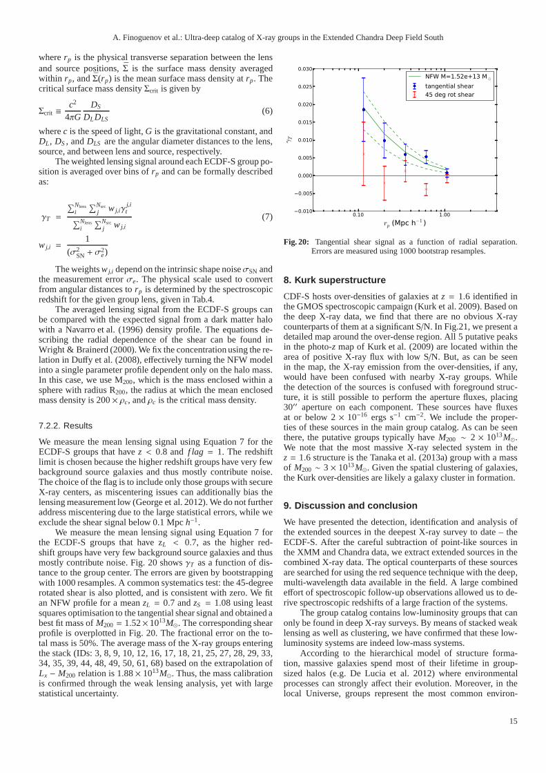
We measure the mean lensing signal using Equation 7 forthe ECDF-S groups that have zL < 0.7, as the higher red-shift groups have very few background source galaxies and thusmostly contribute noise. Fig. 20 showsγT as a function of dis-tance to the group center. The errors are given by bootstrappingwith 1000 resamples. A common systematics test: the 45-degreerotated shear is also plotted, and is consistent with zero. We fitan NFW profile for a meanzL = 0.7 andzS = 1.08 using leastsquares optimisation to the tangential shear signal and obtained abest fit mass ofM200 = 1.52× 10¹³M⊙. The corresponding shearprofile is overplotted in Fig. 20. The fractional error on theto-tal mass is 50%. The average mass of the X-ray groups enteringthe stack (IDs: 3, 8, 9, 10, 12, 16, 17, 18, 21, 25, 27, 28, 29, 33,34, 35, 39, 44, 48, 49, 50, 61, 68) based on the extrapolation ofLx − M200 relation is 1.88× 10¹³M⊙. Thus, the mass calibrationis confirmed through the weak lensing analysis, yet with largestatistical uncertainty.
0.10 1.00
rp (Mpc h−1 )
−0.010
−0.005
0.000
0.005
0.010
0.015
0.020
0.025
0.030
γT
NFW M=1.52e+13 M⊙tangential shear45 deg rot shear
Fig. 20: Tangential shear signal as a function of radial separation.Errors are measured using 1000 bootstrap resamples.
8. Kurk superstructure
CDF-S hosts over-densities of galaxies atz = 1.6 identified inthe GMOS spectroscopic campaign (Kurk et al. 2009). Based onthe deep X-ray data, we find that there are no obvious X-raycounterparts of them at a significant S/N. In Fig.21, we present adetailed map around the over-dense region. All 5 putative peaksin the photo-z map of Kurk et al. (2009) are located within thearea of positive X-ray flux with low S/N. But, as can be seenin the map, the X-ray emission from the over-densities, if any,would have been confused with nearby X-ray groups. Whilethe detection of the sources is confused with foreground struc-ture, it is still possible to perform the aperture fluxes, placing30′′ aperture on each component. These sources have fluxesat or below 2× 10⁻¹⁶ ergs s−1 cm−2. We include the proper-ties of these sources in the main group catalog. As can be seenthere, the putative groups typically haveM200 ∼ 2 × 10¹³M⊙.We note that the most massive X-ray selected system in thez = 1.6 structure is the Tanaka et al. (2013a) group with a massof M200 ∼ 3× 10¹³M⊙. Given the spatial clustering of galaxies,the Kurk over-densities are likely a galaxy cluster in formation.
9. Discussion and conclusion
We have presented the detection, identification and analysis ofthe extended sources in the deepest X-ray survey to date – theECDF-S. After the careful subtraction of point-like sources inthe XMM and Chandra data, we extract extended sources in thecombined X-ray data. The optical counterparts of these sourcesare searched for using the red sequence technique with the deep,multi-wavelength data available in the field. A large combinedeffort of spectroscopic follow-up observations allowed us to de-rive spectroscopic redshifts of a large fraction of the systems.
The group catalog contains low-luminosity groups that canonly be found in deep X-ray surveys. By means of stacked weaklensing as well as clustering, we have confirmed that these low-luminosity systems are indeed low-mass systems.
According to the hierarchical model of structure forma-tion, massive galaxies spend most of their lifetime in group-sized halos (e.g. De Lucia et al. 2012) where environmentalprocesses can strongly affect their evolution. Moreover, in thelocal Universe, groups represent the most common environ-
15
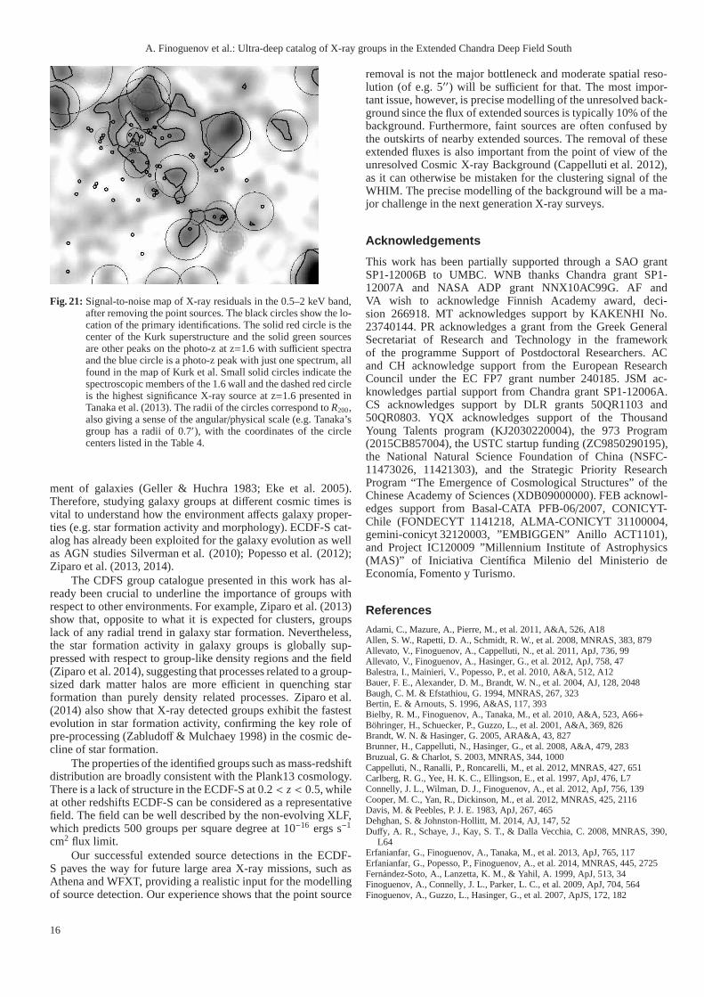
A. Finoguenov et al.: Ultra-deep catalog of X-ray groups in the Extended Chandra Deep Field South
Fig. 21: Signal-to-noise map of X-ray residuals in the 0.5–2 keV band,after removing the point sources. The black circles show thelo-cation of the primary identifications. The solid red circle is thecenter of the Kurk superstructure and the solid green sourcesare other peaks on the photo-z at z=1.6 with sufficient spectraand the blue circle is a photo-z peak with just one spectrum, allfound in the map of Kurk et al. Small solid circles indicate thespectroscopic members of the 1.6 wall and the dashed red circleis the highest significance X-ray source at z=1.6 presented inTanaka et al. (2013). The radii of the circles correspond toR200,also giving a sense of the angular/physical scale (e.g. Tanaka’sgroup has a radii of 0.7′), with the coordinates of the circlecenters listed in the Table 4.
ment of galaxies (Geller & Huchra 1983; Eke et al. 2005).Therefore, studying galaxy groups at different cosmic times isvital to understand how the environment affects galaxy proper-ties (e.g. star formation activity and morphology). ECDF-Scat-alog has already been exploited for the galaxy evolution as wellas AGN studies Silverman et al. (2010); Popesso et al. (2012);Ziparo et al. (2013, 2014).
The CDFS group catalogue presented in this work has al-ready been crucial to underline the importance of groups withrespect to other environments. For example, Ziparo et al. (2013)show that, opposite to what it is expected for clusters, groupslack of any radial trend in galaxy star formation. Nevertheless,the star formation activity in galaxy groups is globally sup-pressed with respect to group-like density regions and the field(Ziparo et al. 2014), suggesting that processes related to agroup-sized dark matter halos are more efficient in quenching starformation than purely density related processes. Ziparo etal.(2014) also show that X-ray detected groups exhibit the fastestevolution in star formation activity, confirming the key role ofpre-processing (Zabludoff & Mulchaey 1998) in the cosmic de-cline of star formation.
The properties of the identified groups such as mass-redshiftdistribution are broadly consistent with the Plank13 cosmology.There is a lack of structure in the ECDF-S at 0.2 < z< 0.5, whileat other redshifts ECDF-S can be considered as a representativefield. The field can be well described by the non-evolving XLF,which predicts 500 groups per square degree at 10−16 ergs s−1
cm2 flux limit.Our successful extended source detections in the ECDF-
S paves the way for future large area X-ray missions, such asAthena and WFXT, providing a realistic input for the modellingof source detection. Our experience shows that the point source
removal is not the major bottleneck and moderate spatial reso-lution (of e.g. 5′′) will be sufficient for that. The most impor-tant issue, however, is precise modelling of the unresolvedback-ground since the flux of extended sources is typically 10% of thebackground. Furthermore, faint sources are often confusedbythe outskirts of nearby extended sources. The removal of theseextended fluxes is also important from the point of view of theunresolved Cosmic X-ray Background (Cappelluti et al. 2012),as it can otherwise be mistaken for the clustering signal of theWHIM. The precise modelling of the background will be a ma-jor challenge in the next generation X-ray surveys.
Acknowledgements
This work has been partially supported through a SAO grantSP1-12006B to UMBC. WNB thanks Chandra grant SP1-12007A and NASA ADP grant NNX10AC99G. AF andVA wish to acknowledge Finnish Academy award, deci-sion 266918. MT acknowledges support by KAKENHI No.23740144. PR acknowledges a grant from the Greek GeneralSecretariat of Research and Technology in the frameworkof the programme Support of Postdoctoral Researchers. ACand CH acknowledge support from the European ResearchCouncil under the EC FP7 grant number 240185. JSM ac-knowledges partial support from Chandra grant SP1-12006A.CS acknowledges support by DLR grants 50QR1103 and50QR0803. YQX acknowledges support of the ThousandYoung Talents program (KJ2030220004), the 973 Program(2015CB857004), the USTC startup funding (ZC9850290195),the National Natural Science Foundation of China (NSFC-11473026, 11421303), and the Strategic Priority ResearchProgram “The Emergence of Cosmological Structures” of theChinese Academy of Sciences (XDB09000000). FEB acknowl-edges support from Basal-CATA PFB-06/2007, CONICYT-Chile (FONDECYT 1141218, ALMA-CONICYT 31100004,gemini-conicyt 32120003, ”EMBIGGEN” Anillo ACT1101),and Project IC120009 ”Millennium Institute of Astrophysics(MAS)” of Iniciativa Cientıfica Milenio del Ministerio deEconomıa, Fomento y Turismo.
ReferencesAdami, C., Mazure, A., Pierre, M., et al. 2011, A&A, 526, A18Allen, S. W., Rapetti, D. A., Schmidt, R. W., et al. 2008, MNRAS, 383, 879Allevato, V., Finoguenov, A., Cappelluti, N., et al. 2011, ApJ, 736, 99Allevato, V., Finoguenov, A., Hasinger, G., et al. 2012, ApJ, 758, 47Balestra, I., Mainieri, V., Popesso, P., et al. 2010, A&A, 512, A12Bauer, F. E., Alexander, D. M., Brandt, W. N., et al. 2004, AJ,128, 2048Baugh, C. M. & Efstathiou, G. 1994, MNRAS, 267, 323Bertin, E. & Arnouts, S. 1996, A&AS, 117, 393Bielby, R. M., Finoguenov, A., Tanaka, M., et al. 2010, A&A, 523, A66+Bohringer, H., Schuecker, P., Guzzo, L., et al. 2001, A&A, 369, 826Brandt, W. N. & Hasinger, G. 2005, ARA&A, 43, 827Brunner, H., Cappelluti, N., Hasinger, G., et al. 2008, A&A,479, 283Bruzual, G. & Charlot, S. 2003, MNRAS, 344, 1000Cappelluti, N., Ranalli, P., Roncarelli, M., et al. 2012, MNRAS, 427, 651Carlberg, R. G., Yee, H. K. C., Ellingson, E., et al. 1997, ApJ, 476, L7Connelly, J. L., Wilman, D. J., Finoguenov, A., et al. 2012, ApJ, 756, 139Cooper, M. C., Yan, R., Dickinson, M., et al. 2012, MNRAS, 425, 2116Davis, M. & Peebles, P. J. E. 1983, ApJ, 267, 465Dehghan, S. & Johnston-Hollitt, M. 2014, AJ, 147, 52Duffy, A. R., Schaye, J., Kay, S. T., & Dalla Vecchia, C. 2008, MNRAS, 390,
L64Erfanianfar, G., Finoguenov, A., Tanaka, M., et al. 2013, ApJ, 765, 117Erfanianfar, G., Popesso, P., Finoguenov, A., et al. 2014, MNRAS, 445, 2725Fernandez-Soto, A., Lanzetta, K. M., & Yahil, A. 1999, ApJ,513, 34Finoguenov, A., Connelly, J. L., Parker, L. C., et al. 2009, ApJ, 704, 564Finoguenov, A., Guzzo, L., Hasinger, G., et al. 2007, ApJS, 172, 182
16
A. Finoguenov et al.: Ultra-deep catalog of X-ray groups in the Extended Chandra Deep Field South
Finoguenov, A., Watson, M. G., Tanaka, M., et al. 2010, MNRAS, 403, 2063Gawiser, E., van Dokkum, P. G., Herrera, D., et al. 2006, ApJS, 162, 1George, M. R., Leauthaud, A., Bundy, K., et al. 2012, ApJ, 757, 2George, M. R., Leauthaud, A., Bundy, K., et al. 2011, ApJ, 742, 125Giacconi, R., Zirm, A., Wang, J., et al. 2002, ApJS, 139, 369Giavalisco, M., Ferguson, H. C., Koekemoer, A. M., et al. 2004, ApJ, 600, L93Giodini, S., Finoguenov, A., Pierini, D., et al. 2012, A&A, 538, A104Giodini, S., Pierini, D., Finoguenov, A., et al. 2009, The Astrophysical Journal,
703, 982Grazian, A., Fontana, A., de Santis, C., et al. 2006, A&A, 449, 951Henry, J. P., Salvato, M., Finoguenov, A., et al. 2010, ApJ, 725, 615Heymans, C., Brown, M. L., Barden, M., et al. 2005, MNRAS, 361, 160Heymans, C., Van Waerbeke, L., Bacon, D., et al. 2006, MNRAS,368, 1323Hickox, R. C. & Markevitch, M. 2006, ApJ, 645, 95Hilton, M., Lloyd-Davies, E., Stanford, S. A., et al. 2010, ApJ, 718, 133Hoekstra, H., Franx, M., Kuijken, K., & Squires, G. 1998, ApJ, 504, 636Jelic, V., Smolcic, V., Finoguenov, A., et al. 2012, MNRAS, 423, 2753Kaiser, N., Squires, G., & Broadhurst, T. 1995, ApJ, 449, 460Koekemoer, A. M., Fruchter, A. S., Hook, R. N., & Hack, W. 2003, in HST
Calibration Workshop : Hubble after the Installation of theACS and theNICMOS Cooling System, ed. S. Arribas, A. Koekemoer, & B. Whitmore,337
Koens, L. A., Maughan, B. J., Jones, L. R., et al. 2013, MNRAS,435, 3231Kurk, J., Cimatti, A., Zamorani, G., et al. 2009, A&A, 504, 331Landy, S. D. & Szalay, A. S. 1993, ApJ, 412, 64Lanzetta, K. M., Yahil, A., & Fernandez-Soto, A. 1996, Nature, 381, 759Leauthaud, A., Finoguenov, A., Kneib, J.-P., et al. 2010, ApJ, 709, 97Leauthaud, A., George, M. R., Behroozi, P. S., et al. 2012, ApJ, 746, 95Lehmer, B. D., Brandt, W. N., Alexander, D. M., et al. 2005, ApJS, 161, 21Lidman, C., Rosati, P., Tanaka, M., et al. 2008, A&A, 489, 981Lloyd-Davies, E. J., Romer, A. K., Mehrtens, N., et al. 2011,MNRAS, 418, 14Luo, B., Bauer, F. E., Brandt, W. N., et al. 2008, ApJS, 179, 19Luppino, G. A. & Kaiser, N. 1997, ApJ, 475, 20MacDonald, E. C., Allen, P., Dalton, G., et al. 2004, MNRAS, 352, 1255Maughan, B. J. 2007, ApJ, 668, 772Meurer, G. R., Lindler, D. J., Blakeslee, J., et al. 2003, in Society of Photo-
Optical Instrumentation Engineers (SPIE) Conference Series, Vol. 4854,Society of Photo-Optical Instrumentation Engineers (SPIE) ConferenceSeries, ed. J. C. Blades & O. H. W. Siegmund, 507–514
Miller, N. A., Bonzini, M., Fomalont, E. B., et al. 2013, ApJS, 205, 13Mirkazemi, M., Finoguenov, A., Pereira, M. J., et al. 2015, ApJ, 799, 60Navarro, J. F., Frenk, C. S., & White, S. D. M. 1996, ApJ, 462, 563Oh, S., Mulchaey, J. S., Woo, J.-H., et al. 2014, ApJ, 790, 43Okabe, N., Zhang, Y.-Y., Finoguenov, A., et al. 2010, ApJ, 721, 875Pacaud, F., Pierre, M., Adami, C., et al. 2007, MNRAS, 382, 1289Paolillo, M., Schreier, E. J., Giacconi, R., Koekemoer, A. M., & Grogin, N. A.
2004, ApJ, 611, 93Pierre, M., Clerc, N., Maughan, B., et al. 2012, A&A, 540, A4Planck Collaboration, Ade, P. A. R., Aghanim, N., et al. 2014, A&A, 571, A26Popesso, P., Biviano, A., Rodighiero, G., et al. 2012, A&A, 537, A58Rafferty, D. A., Brandt, W. N., Alexander, D. M., et al. 2011, ApJ,742, 3Ranalli, P., Comastri, A., Vignali, C., et al. 2013, A&A, 555, A42Rix, H.-W., Barden, M., Beckwith, S. V. W., et al. 2004, ApJS,152, 163Rosati, P., Borgani, S., & Norman, C. 2002, ARA&A, 40, 539Salvato, M., Ilbert, O., Hasinger, G., et al. 2011, ApJ, 742,61Santini, P., Fontana, A., Grazian, A., et al. 2009, A&A, 504,751Schmid, C., Martin, M., Wilms, J., et al. 2010, X-ray Astronomy 2009; Present
Status, Multi-Wavelength Approach and Future Perspectives, 1248, 591Sheth, R. K., Hui, L., Diaferio, A., & Scoccimarro, R. 2001, MNRAS, 325, 1288Silverman, J. D., Mainieri, V., Salvato, M., et al. 2010, ApJS, 191, 124Smolcic, V., Finoguenov, A., Zamorani, G., et al. 2011, MNRAS, 416, L31Struder, L., Aschenbach, B., Brauninger, H., et al. 2001,A&A, 375, L5Tanaka, M., Finoguenov, A., Mirkazemi, M., et al. 2013a, PASJ, 65, 17Tanaka, M., Kodama, T., Kajisawa, M., et al. 2007, MNRAS, 377, 1206Tanaka, M., Toft, S., Marchesini, D., et al. 2013b, ApJ, 772,113Taylor, J. E., Massey, R. J., Leauthaud, A., et al. 2012, ApJ,749, 127Turner, M. J. L., Abbey, A., Arnaud, M., et al. 2001, A&A, 365,L27Vikhlinin, A., Burenin, R. A., Ebeling, H., et al. 2009, ApJ,692, 1033Vikhlinin, A., McNamara, B. R., Forman, W., et al. 1998, ApJ,502, 558Wright, C. O. & Brainerd, T. G. 2000, ApJ, 534, 34Xue, Y. Q., Luo, B., Brandt, W. N., et al. 2011, ApJS, 195, 10Ziparo, F., Popesso, P., Biviano, A., et al. 2013, MNRAS, 434, 3089Ziparo, F., Popesso, P., Finoguenov, A., et al. 2014, MNRAS,437, 458
17
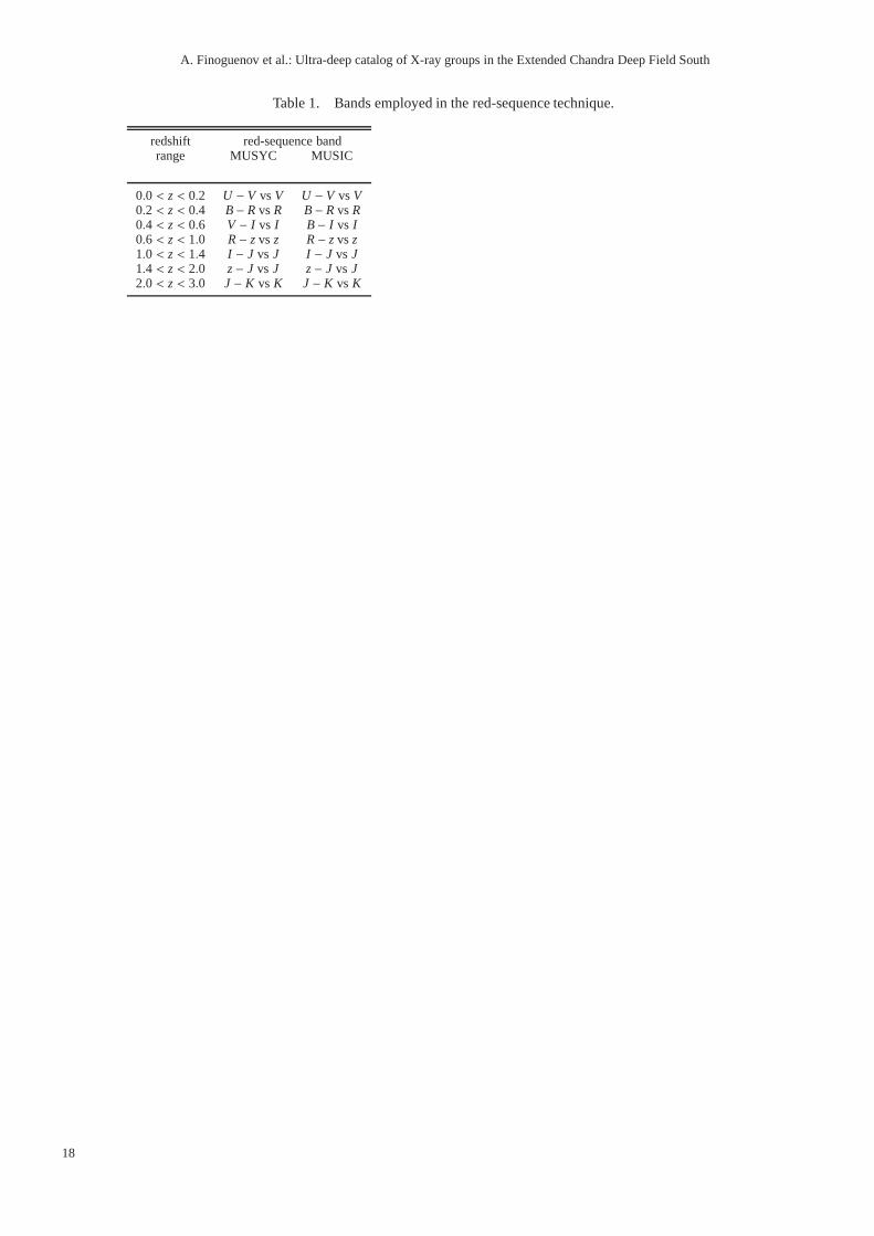
A. Finoguenov et al.: Ultra-deep catalog of X-ray groups in the Extended Chandra Deep Field South
Table 1. Bands employed in the red-sequence technique.
redshift red-sequence bandrange MUSYC MUSIC
0.0 < z< 0.2 U − V vs V U − V vs V0.2 < z< 0.4 B− Rvs R B− Rvs R0.4 < z< 0.6 V − I vs I B − I vs I0.6 < z< 1.0 R− zvs z R− zvs z1.0 < z< 1.4 I − J vs J I − J vs J1.4 < z< 2.0 z− J vs J z− J vs J2.0 < z< 3.0 J − K vs K J − K vs K
18
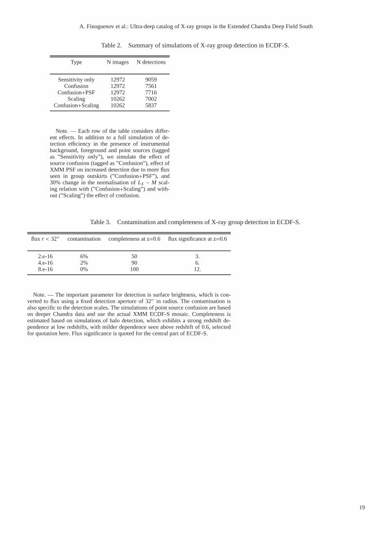
A. Finoguenov et al.: Ultra-deep catalog of X-ray groups in the Extended Chandra Deep Field South
Table 2. Summary of simulations of X-ray group detection in ECDF-S.
Type N images N detections
Sensitivity only 12972 9059Confusion 12972 7561
Confusion+PSF 12972 7716Scaling 10262 7002
Confusion+Scaling 10262 5837
Note. — Each row of the table considers differ-ent effects. In addition to a full simulation of de-tection efficiency in the presence of instrumentalbackground, foreground and point sources (taggedas ”Sensitivity only”), we simulate the effect ofsource confusion (tagged as ”Confusion”), effect ofXMM PSF on increased detection due to more fluxseen in group outskirts (”Confusion+PSF”), and30% change in the normalisation ofLX − M scal-ing relation with (”Confusion+Scaling”) and with-out (”Scaling”) the effect of confusion.
Table 3. Contamination and completeness of X-ray group detection in ECDF-S.
flux r < 32′′ contamination completeness at z=0.6 flux significance at z=0.6
2.e-16 6% 50 3.4.e-16 2% 90 6.8.e-16 0% 100 12.
Note. — The important parameter for detection is surface brightness, which is con-verted to flux using a fixed detection aperture of 32′′ in radius. The contamination isalso specific to the detection scales. The simulations of point source confusion are basedon deeper Chandra data and use the actual XMM ECDF-S mosaic. Completeness isestimated based on simulations of halo detection, which exhibits a strong redshift de-pendence at low redshifts, with milder dependence seen above redshift of 0.6, selectedfor quotation here. Flux significance is quoted for the central part of ECDF-S.
19
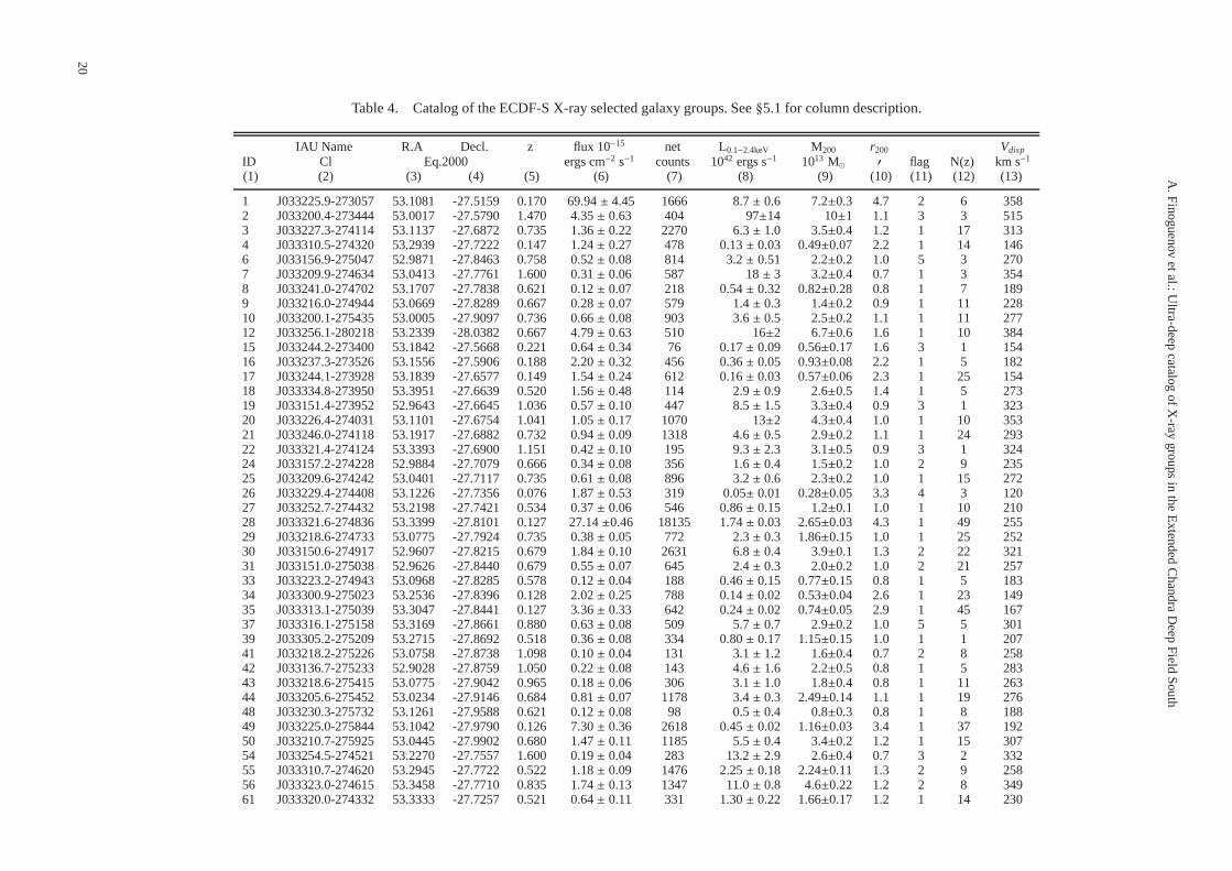
A.F
inoguenovetal.:U
ltra-deepcatalog
ofX-ray
groupsin
the
Extended
Chandra
Deep
Field
South
Table 4. Catalog of the ECDF-S X-ray selected galaxy groups.See§5.1 for column description.
IAU Name R.A Decl. z flux 10−15 net L0.1−2.4keV M200 r200 Vdisp
ID Cl Eq.2000 ergs cm−2 s−1 counts 1042 ergs s−1 1013 M⊙ ′ flag N(z) km s−1
(1) (2) (3) (4) (5) (6) (7) (8) (9) (10) (11) (12) (13)
1 J033225.9-273057 53.1081 -27.5159 0.170 69.94± 4.45 1666 8.7± 0.6 7.2±0.3 4.7 2 6 3582 J033200.4-273444 53.0017 -27.5790 1.470 4.35± 0.63 404 97±14 10±1 1.1 3 3 5153 J033227.3-274114 53.1137 -27.6872 0.735 1.36± 0.22 2270 6.3± 1.0 3.5±0.4 1.2 1 17 3134 J033310.5-274320 53.2939 -27.7222 0.147 1.24± 0.27 478 0.13± 0.03 0.49±0.07 2.2 1 14 1466 J033156.9-275047 52.9871 -27.8463 0.758 0.52± 0.08 814 3.2± 0.51 2.2±0.2 1.0 5 3 2707 J033209.9-274634 53.0413 -27.7761 1.600 0.31± 0.06 587 18± 3 3.2±0.4 0.7 1 3 3548 J033241.0-274702 53.1707 -27.7838 0.621 0.12± 0.07 218 0.54± 0.32 0.82±0.28 0.8 1 7 1899 J033216.0-274944 53.0669 -27.8289 0.667 0.28± 0.07 579 1.4± 0.3 1.4±0.2 0.9 1 11 22810 J033200.1-275435 53.0005 -27.9097 0.736 0.66± 0.08 903 3.6± 0.5 2.5±0.2 1.1 1 11 27712 J033256.1-280218 53.2339 -28.0382 0.667 4.79± 0.63 510 16±2 6.7±0.6 1.6 1 10 38415 J033244.2-273400 53.1842 -27.5668 0.221 0.64± 0.34 76 0.17± 0.09 0.56±0.17 1.6 3 1 15416 J033237.3-273526 53.1556 -27.5906 0.188 2.20± 0.32 456 0.36± 0.05 0.93±0.08 2.2 1 5 18217 J033244.1-273928 53.1839 -27.6577 0.149 1.54± 0.24 612 0.16± 0.03 0.57±0.06 2.3 1 25 15418 J033334.8-273950 53.3951 -27.6639 0.520 1.56± 0.48 114 2.9± 0.9 2.6±0.5 1.4 1 5 27319 J033151.4-273952 52.9643 -27.6645 1.036 0.57± 0.10 447 8.5± 1.5 3.3±0.4 0.9 3 1 32320 J033226.4-274031 53.1101 -27.6754 1.041 1.05± 0.17 1070 13±2 4.3±0.4 1.0 1 10 35321 J033246.0-274118 53.1917 -27.6882 0.732 0.94± 0.09 1318 4.6± 0.5 2.9±0.2 1.1 1 24 29322 J033321.4-274124 53.3393 -27.6900 1.151 0.42± 0.10 195 9.3± 2.3 3.1±0.5 0.9 3 1 32424 J033157.2-274228 52.9884 -27.7079 0.666 0.34± 0.08 356 1.6± 0.4 1.5±0.2 1.0 2 9 23525 J033209.6-274242 53.0401 -27.7117 0.735 0.61± 0.08 896 3.2± 0.6 2.3±0.2 1.0 1 15 27226 J033229.4-274408 53.1226 -27.7356 0.076 1.87± 0.53 319 0.05± 0.01 0.28±0.05 3.3 4 3 12027 J033252.7-274432 53.2198 -27.7421 0.534 0.37± 0.06 546 0.86± 0.15 1.2±0.1 1.0 1 10 21028 J033321.6-274836 53.3399 -27.8101 0.127 27.14±0.46 18135 1.74± 0.03 2.65±0.03 4.3 1 49 25529 J033218.6-274733 53.0775 -27.7924 0.735 0.38± 0.05 772 2.3± 0.3 1.86±0.15 1.0 1 25 25230 J033150.6-274917 52.9607 -27.8215 0.679 1.84± 0.10 2631 6.8± 0.4 3.9±0.1 1.3 2 22 32131 J033151.0-275038 52.9626 -27.8440 0.679 0.55± 0.07 645 2.4± 0.3 2.0±0.2 1.0 2 21 25733 J033223.2-274943 53.0968 -27.8285 0.578 0.12± 0.04 188 0.46± 0.15 0.77±0.15 0.8 1 5 18334 J033300.9-275023 53.2536 -27.8396 0.128 2.02± 0.25 788 0.14± 0.02 0.53±0.04 2.6 1 23 14935 J033313.1-275039 53.3047 -27.8441 0.127 3.36± 0.33 642 0.24± 0.02 0.74±0.05 2.9 1 45 16737 J033316.1-275158 53.3169 -27.8661 0.880 0.63± 0.08 509 5.7± 0.7 2.9±0.2 1.0 5 5 30139 J033305.2-275209 53.2715 -27.8692 0.518 0.36± 0.08 334 0.80± 0.17 1.15±0.15 1.0 1 1 20741 J033218.2-275226 53.0758 -27.8738 1.098 0.10± 0.04 131 3.1± 1.2 1.6±0.4 0.7 2 8 25842 J033136.7-275233 52.9028 -27.8759 1.050 0.22± 0.08 143 4.6± 1.6 2.2±0.5 0.8 1 5 28343 J033218.6-275415 53.0775 -27.9042 0.965 0.18± 0.06 306 3.1± 1.0 1.8±0.4 0.8 1 11 26344 J033205.6-275452 53.0234 -27.9146 0.684 0.81± 0.07 1178 3.4± 0.3 2.49±0.14 1.1 1 19 27648 J033230.3-275732 53.1261 -27.9588 0.621 0.12± 0.08 98 0.5± 0.4 0.8±0.3 0.8 1 8 18849 J033225.0-275844 53.1042 -27.9790 0.126 7.30± 0.36 2618 0.45± 0.02 1.16±0.03 3.4 1 37 19250 J033210.7-275925 53.0445 -27.9902 0.680 1.47± 0.11 1185 5.5± 0.4 3.4±0.2 1.2 1 15 30754 J033254.5-274521 53.2270 -27.7557 1.600 0.19± 0.04 283 13.2± 2.9 2.6±0.4 0.7 3 2 33255 J033310.7-274620 53.2945 -27.7722 0.522 1.18± 0.09 1476 2.25± 0.18 2.24±0.11 1.3 2 9 25856 J033323.0-274615 53.3458 -27.7710 0.835 1.74± 0.13 1347 11.0± 0.8 4.6±0.22 1.2 2 8 34961 J033320.0-274332 53.3333 -27.7257 0.521 0.64± 0.11 331 1.30± 0.22 1.66±0.17 1.2 1 14 230
20
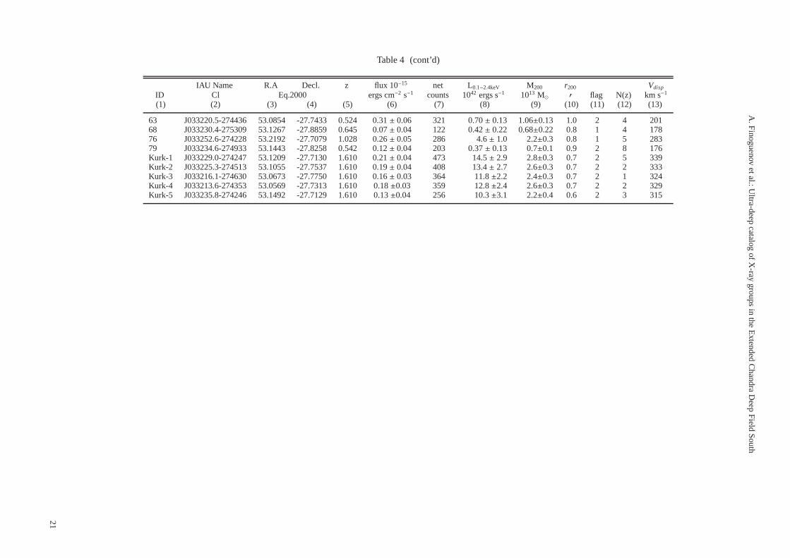
A.F
inoguenovetal.:U
ltra-deepcatalog
ofX-ray
groupsin
the
Extended
Chandra
Deep
Field
South
Table 4 (cont’d)
IAU Name R.A Decl. z flux 10−15 net L0.1−2.4keV M200 r200 Vdisp
ID Cl Eq.2000 ergs cm−2 s−1 counts 1042 ergs s−1 1013 M⊙ ′ flag N(z) km s−1
(1) (2) (3) (4) (5) (6) (7) (8) (9) (10) (11) (12) (13)
63 J033220.5-274436 53.0854 -27.7433 0.524 0.31± 0.06 321 0.70± 0.13 1.06±0.13 1.0 2 4 20168 J033230.4-275309 53.1267 -27.8859 0.645 0.07± 0.04 122 0.42± 0.22 0.68±0.22 0.8 1 4 17876 J033252.6-274228 53.2192 -27.7079 1.028 0.26± 0.05 286 4.6± 1.0 2.2±0.3 0.8 1 5 28379 J033234.6-274933 53.1443 -27.8258 0.542 0.12± 0.04 203 0.37± 0.13 0.7±0.1 0.9 2 8 176Kurk-1 J033229.0-274247 53.1209 -27.7130 1.610 0.21± 0.04 473 14.5± 2.9 2.8±0.3 0.7 2 5 339Kurk-2 J033225.3-274513 53.1055 -27.7537 1.610 0.19± 0.04 408 13.4± 2.7 2.6±0.3 0.7 2 2 333Kurk-3 J033216.1-274630 53.0673 -27.7750 1.610 0.16± 0.03 364 11.8±2.2 2.4±0.3 0.7 2 1 324Kurk-4 J033213.6-274353 53.0569 -27.7313 1.610 0.18±0.03 359 12.8±2.4 2.6±0.3 0.7 2 2 329Kurk-5 J033235.8-274246 53.1492 -27.7129 1.610 0.13±0.04 256 10.3±3.1 2.2±0.4 0.6 2 3 315
21