Modeling and Simulation of a Coupled Double-Loop-Cooling System for PEM-Fuel Cell Stack Cooling

Martin Schultze, Michael Kirsten, Sven Helmker and Joachim Horn Institute for Control Engineering

Helmut-Schmidt-University Hamburg D-22043 Hamburg, Germany

Abstract—PEM (Polymer electrolyte membrane) fuel cell systems are very efficient energy converters. They generate electrical power, low oxygen concentration cathode exhaust gas, water as well as heat. The fuel cell technology has become very attractive for the use on aircraft where it may serve as a replacement for the auxiliary power unit currently being used for generating electrical power. For the use on aircraft coupled double-loop-cooling systems are investigated as different coolants can be used for inner and outer cooling system. As fuel cell electrical power is nonlinearly dependent on stack temperature and current, a cooling temperature control is required.

In this study a nonlinear simulation model of a coupled double-loop-cooling system is presented. The effectiveness-NTU method is used to model the intercooler that couples inner and outer cooling loop. This method has the advantage that outlet temperatures are obtained explicitly based on inlet coolant temperatures and cooling mass flows. The model is valid over the entire operating range of the hydrogen fed fuel cell system. Subsequently, a linear controller with feedforward control is proposed to control for the stack inlet cooling temperature.

PEM fuel cell system model; nonlinear heat exchanger model; model identification; fuel cell temperature control

I. INTRODUCTION For aircraft applications the fuel cell technology is

investigated regarding to its multifunctional use. One of its main aspects is the use of oxygen depleted cathode exhaust air (ODA) for tank inerting [1]. For this purpose the oxygen content needs to be close or less than 10% (vol.) [2]. Another and certainly one of the most important aspects of the multifunctional use is electrical power generation. So far, auxiliary power units (APU) generate electrical power for the use on aircraft during ground operations. An APU, though, is a significant source of green house gases such as CO2 and NOx and noise. Therefore, hydrogen-gas fed PEM fuel cell systems are studied as a replacement for APUs to significantly reduce these pollutants. Among the different types of fuel cells, PEM fuel cells are the most suitable ones for dynamic applications. Nonetheless, proper fuel cell system operation such as a well humidified membrane or a proper supply of reactant gases and well kept gas pressure is central for a maximum fuel cell lifetime [3]. In this study a fuel cell system with anode hydrogen recirculation for stack humidification is used. Proper fuel and air supply as well as the temperature difference across

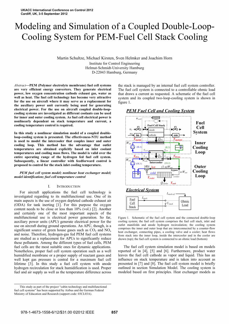
the stack is managed by an internal fuel cell system controller. The fuel cell system is connected to a controllable ohmic load that draws a current as requested. A schematic of the fuel cell system and its coupled two-loop-cooling system is shown in figure 1.

PEM Fuel Cell and Cooling System

H2

Fuel Cell Stackanode

cathode

TICin

Air

Tstackin

.QIC

Qcooler.

.QFC

cooler

bypass

Intercoolervalve hot

Tstackout

TICout

Tcooler

cold

Fuel Cell

System

Inner Cooling

Loop

Outer Cooling

LoopuWext

(1-u)Wext

(IL1) (IL2)

(OL1) (OL2)

Wint

Wext WextIC

WextH2

Th,out Th,in

Tc,outTc,in

im om

Tamb

Electrical System

Fuel Cell

Stack

OhmicLoad

IstackUstack

Istack,ref

Figure 1. Schematic of the fuel cell system and the connected double-loop cooling system; the fuel cell system comprises the fuel cell stack, inlet and outlet manifolds and anode hydrogen recirculation; the cooling system comprises the inner and outer loop that are interconnected by a counter-flow heat exchanger, connecting pipes, a cooling valve and a cooler; heat flows from stack into the inner loop, inside the intercooler and in the cooler are shown (top); the fuel cell system is connected to an ohmic load (bottom)

The fuel cell system simulation model is based on models reported of in [4], [5] and [6]. Furthermore, product water leaves the fuel cell cathode as vapor and liquid. This has an influence on stack temperature and is taken into account as presented in [7] and [8]. The fuel cell system model is briefly outlined in section Simulation Model. The cooling system is modeled based on first principles. Heat exchanger models as

This study as part of the project “cabin technology and multifunctional fuel cell systems” has been supported by Airbus and the German Federal Ministry of Education and Research (support code: 03CL03A).

857

UKACC International Conference on Control 2012 Cardiff, UK, 3-5 September 2012

978-1-4673-1558-6/12/$31.00 ©2012 IEEE

proposed in [9] and [6] are restricted on operating range. The effectiveness-NTU method [10] provides nonlinear models for several designs of heat exchangers. Ref. [11] uses this approach for a single-loop cooling system of an automotive fuel cell system assuming constant heat exchanger effectiveness. Constant effectiveness, however, might not hold true for the entire operating range. Here, the effectiveness-NTU method with mass flow dependent effectiveness is used to develop an intercooler model for the coupled double-loop-cooling system. The fuel cell system and intercooler model have been fit to experimental data, which is presented in section Model Identification. Actuating the cooling valve in the outer loop influences the stack inlet temperature in the inner cooling loop. To operate the fuel cell system at a certain stack inlet temperature a temperature controller with feedforward control is proposed in section Controller Design. A simulation of the nonlinear fuel cell and cooling system model with temperature controller are presented in section Simulation results.

II. SIMULATION MODEL The overall system simulation model consists of a model of

the fuel cell system, a model of its internal fuel cell system controller and a model of the controllable ohmic electrical load to which the fuel cell system is connected. A list of the model parameters is given in table 1 at the end of this paper. Inlet air is taken from an air pressure tank that is filled by a compressor. After compression air is cooled, dried and oil-filtered.

A. Fuel Cell System Model The fuel cell system model comprises the fuel cell stack, a

mass flow controller (MFC) for cathode air supply and the anode hydrogen recirculation for better hydrogen utilization and stack humidification. The internal fuel cell system controller operates the mass flow controller such that it delivers an air mass flow as specified by stoichiometry and stack current drawn. Furthermore, the internal controller operates the cooling pump in the inner cooling loop to set the reference temperature difference across the fuel cell stack. Inlet air is modeled as a dry and ideal gas consisting of 21% (vol.) oxygen and 79% (vol.) nitrogen. It has constant temperature.

1) Inlet Manifold Model Inlet manifold pressure pim (1) is gained by a pressure

differential equation (γ =1.4 [5]). In- and outlet temperature are assumed to be equal and constant. Flow Wim of dry air exiting the manifold is modeled by a linear nozzle equation (2) with nozzle constant kim and the pressure difference of manifold and cathode pressure pca. Mass flow of dry air WMFC (3) entering the manifold is supplied by a mass flow controller, which is modeled as a first order transfer function with time constant TMFC. The mass flow reference is calculated using the reference stoichiometry λref and the stack current Istack being drawn.

( )

2) Outlet Manifold Model Vapor mass flow is obtained by water loading (4) of the dry

gas mass flow. Water loading depends on total gas pressure pi and vapor partial pressure pi,v (5), which solely depends on temperature [12]. Mass flows of water vapor Wca,v, oxygen depleted air Wca,oda and liquid water Wca,l are supplied to the outlet manifold at stack temperature Tstack. The manifold is considered perfectly insulated. Mass flows Wom,v, Wom,oda and Wom,l exit directly to the ambient environment and are governed by a linear nozzle equation with constant kom and manifold and ambient pressure difference (6). The flow of liquid water leaving the manifold (7) is modeled to be dependent on the gas mass flow, the liquid water mass mom,l and a constant δl [7].

v

air

ivi

ivi R

Rpp

pX

,

,

−= (4)

310611657.0431.237

99.41022799.17exp ×⎟⎠⎞

⎜⎝⎛

+−=ϑ

satvp (5)

( )ambomomom ppkW −= (6)

lomomllom mWW ,, δ= (7)

Partial pressures of dry gas pom,oda and vapor pom,v are gained by a mass balance and the ideal gas law (8) with manifold volume Vom and the vapor gas constant Rv. ODA is approximated as air with gas constant Roda=Rair. Condensation is considered happening instantaneously leading to the condensate mass mom,l. The outlet manifold pressure is the sum of oda and vapor partial pressures pom = pom,oda + pom,v.

,

,

,,,,2,

,,,

lomvomlcavcaOHom

odaomodacaodaom

WWWWdt

dm

WWdt

dm

−−+=

−=

omom

omvom

omom

odaom

WX

XW

WX

W

+=

+=

1

11

,

,

odaomom

odaomodaom m

VRT

p ,, = (8)

⎟⎟⎠

⎞⎜⎜⎝

⎛=

om

omvOHomom

satvvom V

TRmTpp 2,, ),(min (9)

⎟⎟⎠

⎞⎜⎜⎝

⎛−=

omv

omom

satvOHomlom TR

VTpmm )(,0max 2,,

(10)

3) Fuel Cell Stack Electrical Model The stack voltage Ustack = ncells Ucell is the sum of all ncells

cell voltages. The cell voltage is modeled as Ucell = Urev –ηact –ηΩ (11) with the reversible cell voltage Urev, activation loss ηact [13] and ohmic loss ηΩ [14]. The membrane thickness is given by dm and the active surface area by Asfc. Parameters ζ1,…ζ4 and b1,…b3 have been identified using experimental data.

imMFCimim

airim WWTVR

dtdp

−=γ (1)

( )caimimim ppkW −= (2)

⎥⎦

⎤⎢⎣

⎡⎟⎠⎞

⎜⎝⎛ +

+=

Fn

MMIsT

W cellsNOrefstack

MFCMFC 421.0

79.01

122λ (3)

( ) ( )0

2

0

2 lnln103.415.2981085.0229.1 2153

pp

pp

stackstackrevOHTTU +⋅+−⋅−= −−

( )( ) ( )stackstackT

Ostackstackact ITepTT stack ln1008.5/ln 46/498

2321 ζζζζη +⋅++= −

( ) sfcAstackIT

b

bmbmd

stacke⎟⎟⎠

⎞⎜⎜⎝

⎛−−

−Ω =1

3031

3

21λη (11)

4) Fuel Cell Stack Thermal Model An energy balance (12) leads to the fuel cell stack

temperature Tstack. The stack has a heat capacity of Cst. The heat generated through the chemical reaction is given by the

858

chemical energy of hydrogen (HHV) and stack electrical energy. The stack is cooled by convective cooling with coolant mass flow Wcool = Wint and specific heat capacity ccool. The coolant stack inflow temperature is Tstackin. The coolant leaves the stack at stack temperature. Air, cathode water, vapor and oda gas are assumed to leave the stack at stack temperature as well. Air enters the stack at temperature Tim. Oda gas is approximated as air with specific heat capacity coda = cair. The stack is very well insulated. So, heat transfer to surroundings is neglected. Enthalpy of evaporation is h0.

( )( )

( ) ( )( ) (( )00,0,

00

48.1

TTchWTTcWTTcWTTcW

TTcW

IUndt

dTC

stackvvcastackllca

stackodaodaimairim

stackstackincoolcool

stackstackcellsst

st

−+−−−−−−+

−+

−=

)

(12)

5) Fuel Cell Stack Anode and Cathode Model Anode pressure pan = pH2 + pan,v is the sum of hydrogen and

vapor partial pressures and is governed by mass conservation (13) and the ideal gas law with RH2 being the hydrogen gas constant. In operation a mass flow WH2rct = (MH2 Istack ncells)/(2F) of hydrogen is consumed. The stack is operated dead-ended and the system behavior is mimicked by a proportional controller for anode pressure pan with hydrogen inlet mass flow WH2in, anode reference pressure pan_ref and controller gain kan (14). Condensation is modeled happening instantaneously [5] if the vapor pressure exceeds saturation vapor pressure. The mass of condensate and the vapor partial pressure are modeled according to (9) and (10) with water mass (13). The anode water activity aan is modeled as aan = pan,v/pv

sat.

memOHan W

dtdm

−=2, and ( rctHinHan

HstackH WWV

RTdt

dp22

22 −=

6) Fuel Cell Stack Membrane Model Membrane material is Nafion®. The membrane water mass

flow Wmem (17) is caused by gradient driven diffusion and electro-osmotic drag of water from anode to cathode [14]. Diffusion constant Ddiff depends on the membrane hydration λmem and stack temperature (18). The membrane water activity amem is modeled as the average between cathode and anode water activity [14] (with j=mem, ca, an).

⎟⎠⎞⎜

⎝⎛ −= −

mdanca

diffdryMdry

FsfcAstackI

memcellswsfcmem DnMAW λλρλ 22

5.2 (17)

( ) ( ) 6103000671.020264.033.0563.2

/1303/12416 −−+−

− ⋅= memmemmemT

diffsteD λλλ

( )⎪⎩

⎪⎨⎧

≤<−+≤<+−+

=3114.114100.3685.3981.17043.0 32

aaaaaa

j

jjjjλ

(18)

7) Electrical Load Model The stack is connected to a controllable ohmic load

drawing a current as requested by a reference. An internal controller quickly adjusts the load resistance. To prevent numerical problems, the load is modeled as a first order transfer function with time constant TL.

B. Cooling System Model As shown in figure 1 the cooling system consists of an

inner and an outer cooling loop that are interconnected by an counter-flow heat exchanger also called intercooler. In the inner loop pipes connect the intercooler and the stack.

) (13)

( )anrefananinH ppkW −= _2 (14)

The cathode inlet mass flows of oxygen and nitrogen are governed by the mass fractions xO2 and xN2 assuming dry inlet air consisting of 21% of oxygen and 79% of nitrogen. The cathode exit mass flow Wca is modeled as a 3-phase-flow (15) and is governed by a linear nozzle equation similar to (2) with constant kca and pressure difference (pca - pom). Liquid water mass flow Wca,l is modeled according to (7). Cathode pressure pca = pO2 + pN2 + pca,v is the sum of oxygen, nitrogen and vapor partial pressures and is governed by mass conservation (16) and the ideal gas law [5]. In operation a mass flow WO2rct = (MO2 Istack ncells)/(4F) of oxygen is consumed and WH2Orct = (MH2O Istack ncells)/(2F) of water is generated. Condensation happens instantaneously. The vapor partial pressure and liquid mass in the cathode is modeled according to (9) and (10) using the water mass mca,H2O in (16).

imN

O

Nim

Oim Wxx

WW

⎥⎦

⎤⎢⎣

⎡=

⎥⎥⎦

⎤

⎢⎢⎣

⎡

2

2

2,

2, and ca

CA

mmm

mmm

CAvca

Nca

Oca

WX

XW

WW

NO

N

NO

O

⎥⎥⎥⎥

⎦

⎤

⎢⎢⎢⎢

⎣

⎡

+=

⎥⎥⎥

⎦

⎤

⎢⎢⎢

⎣

⎡

+

+

22

2

22

2

11

,

2,

2, (15)

2,2,2

2,22,2

,,22,

NcaNimN

OcarctOOimO

lcavcaOrctHmemOHca

WWdt

dm

WWWdt

dm

WWWWdt

dm

−=

−−=

−−+=

,

ca

NstackNN

ca

OstackOO

VRTmp

VRTmp

222

222

=

= (16)

1) Inner Cooling Loop Model The cooling pump in the internal cooling circuit is

controlled such that the cooling temperature difference across the stack equals the reference signal given by the stack manufacturer. The pump generates a coolant mass flow Wint, which is limited to a minimum of Wint,min and a maximum of Wint,max. The cooling pump controller is modeled as a proportional and integral controller with anti-windup to prevent integrator windup. The pipes are modeled according to [13] and are considered perfectly insulated (20) with specific heat capacity cint and mpipe,i being the mass of coolant in pipe i, the coolant inlet temperature Tpipein,i and the pipe outlet temperature Tpipe,i. Using notation of figure 1 the temperature of pipe IL1 is Tstackin and of pipe IL2 is Tstackout. The indices for the model equations (20) are i=IL1, IL2.

( ) (20) ipipeipipein

ipipeipipe TTcW

dtdT

cm ,,intint,

int, −=

2) Outer Cooling Loop Model The outer loop consists of an air-cooled heat exchanger

(cooler) that cools the coolant to a temperature of Tcooler and pipes that connect the cooler with the intercooler. In a cooling valve warm coolant from the intercooler and cold cooling fluid from the cooler can be mixed. Warm coolant bypasses the cooler such that is does not cool down. As the bypass pipe is very short as compared to the other pipes its dynamics are neglected. The cooler is modeled as a pipe as well (21). The heat transferred to the surroundings is modeled by the coefficient kcooler and the difference of cooler to ambient temperature Tamb. The mass flow in the external cooling loop is Wext and the specific heat capacity of the coolant is cext. Using

859

notation of figure 1 the temperature of pipe OL1 is TICin and of pipe OL2 is TICout. The indices for the model equations (21) are i=OL1, OL2.

( )

( ) ( ambcoolercoolercoolerICoutextextvalvecooler

extcooler

ipipeipipeinextextipipe

extipipe

TTkTTcWud

)t

dTcm

TTcWdt

dTcm

−−−=

−= ,,,

, (21)

In pipe OL2 the coolant for the hydrogen recirculation pump mixes with the coolant of the intercooler outflow. This temperature mixture is modeled by a stationary energy balance (22) with thermal input of the hydrogen pump and assuming that the mass flow through the recirculation pump WextH2 is 6% of Wext. Tc,out is the intercooler outlet temperature. The mass flow through the intercooler WextIC is taken as 94% of the mass flow in the external cooling loop.

outcextICextextH

pumpHICinextHICoutext TW

cWQ

TWTW ,2

22 +⎟

⎟⎠

⎞⎜⎜⎝

⎛+= (22)

3) Cooling Valve Model The mixing temperature of the cooling valve is modeled by

a stationary energy equation (23) as the mixing process is considered very fast. The valve splits the mass flow through cooler and bypass given by its actual position uvalve.

( ) ICoutextvalvecoolerextvalveOLpipeinext TWuTWuTW −+= 11, (23)

The cooling valve has limited dynamics. This results in a limited speed of opening and closing the valve. For small changes in position it behaves linearly. It is modeled having a constant opening and closing speed dumax for large changes and behaves like a first order transfer function for small changes in valve position (24). Reference position is uvalve,ref.

( )( )

( )∫

−<−−−

>−=

max,max

,

max,max

duuukduotherwiseuuk

duuukdu

dtdu

valverefvalvevalve

valverefvalvevalve

valverefvalvevalvevalve (24)

4) Intercooler Model The counter-flow heat exchanger that connects the inner

and outer cooling loop is considered static. This assumption is motivated by the high mass flows in the cooling system and the small coolant mass inside the intercooler as compared to the entire cooling system. For modeling counter-flow heat exchangers the effectiveness NTU method [10] has shown very good results. NTU is the number of transfer units, which is an important parameter in heat exchanger design and modeling. The effectiveness NTU is advantageous as outlet temperatures are calculated explicitly on inlet temperatures and cooling mass flows. Heat flow is gained by the inlet temperature differences, the minimum heat capacity flow and the effectiveness ε. The outlet temperatures (25) are gained by the heat capacity flow of the hot side Ch=Wint cint and the cold side Cc=WextIC cext. The outlet temperatures are Tc,out and Th,out for cold and hot side. The inlet temperatures are Tc,in=TICin and Th,in=Tstackout.

( )

( )incinhh

inhouth

incinhc

incoutc

TTCC

TT

TTCC

TT

,,min

,,

,,min

,,

−−=

−+=

ε

ε (25)

( )ch CCC ,minmin = , ( )ch CCC ,maxmax = , max

min*

CCC = ,

minCUANTU =

The heat exchanger effectiveness ε is obtained by (26). UA is the parameter describing the heat transfer.

( )( )( )( )⎪

⎪⎩

⎪⎪⎨

⎧

−−−−−−

=+=

otherwiseCNTUC

CNTU

CNTU

NTU

**

*

*

1exp11exp1

11ε (26)

III. MODEL IDENTIFICATION As shown in the previous paragraphs, the fuel cell system

model as well as the cooling system model has parameters describing the plant geometry such as manifold volumes and coolant masses and parameters for mass flows, polarization curve and the intercooler. Parameters ζ1,…ζ4 and b1,…b3 for the polarization curve, kim, kca, kom and kan for the mass flows have been identified by a least square error minimization such that simulated inlet and outlet manifold as well as cathode and anode pressure and simulated stack voltage fit to experimental data. Cathode pressure cannot be measured, therefore, it is assumed as the arithmetic mean of the inlet and outlet manifold pressures. The objective function (27) has scaling factors for pressure μp and voltage μU such that quadratic errors of the same order are gained.

( ) ( )( ) (( )2,,exp,,

2,,exp,,

2,,exp,,

2,,exp,,

2,,exp,,,

isimstackistackU

isimanianpisimomiomp

isimcaicapisimimiimpiFCS

UU

pppp

ppppJ

−+

−+−+

−+−=

μ

μμ

μμ

)

∑=i

iFCSFCS JJ , (27)

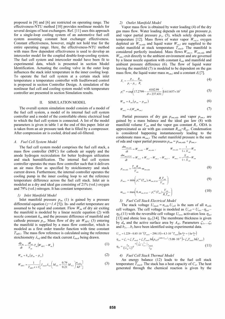
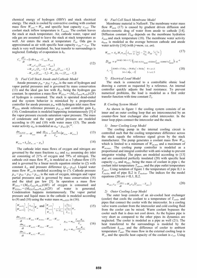
Simulation results of the stationary fuel cell system model after identification of the polarization curve for different sets of stoichiometry and stack inlet cooling temperature are shown in figure 2. The results for inlet as well as outlet manifold and anode pressure are shown in figure 3. As the comparison between experimental data and simulation model shows, the model fits the experimental data very well.

0 50 100 150 200 250 300 350 400 45060

65

70

75

80

85

90

95

stack current [A]

stac

k vo

ltage

(nor

mal

ized

) [%

]

sim (stoic low, Tstackin=45°C)sim (stoic high,Tstackin=45°C)sim (stoic low, Tstackin=58°C)sim (stoic high,Tstackin=58°C)exp (stoic low, Tstackin=45°C)exp (stoic high,Tstackin=45°C)exp (stoic low, Tstackin=58°C)exp (stoic high,Tstackin=58°C)

Figure 2. Comparison of experimental and simulation model fuel cell stack polarization curves for different sets of stack inlet temperature (45 and 58°C) and cathode stoichiometry (high and low stoic)

860

0 2 4 6 8 10 12 14 160

10

20

30

40

50

60

70

80

trial number

rela

tive

pres

sure

(nor

mal

ized

) [%

]

Tstackin=58°CTstackin=45°C

100A 200A 300A 400A 100A 200A 300A 400A

stoic high

stoic low

im (exp)im (sim)om (exp)om (sim)an (exp)an (sim)

Figure 3. Comparison of experimental and simulation inlet manifold (im), outlet manifold (om) and anode (an) pressures; 16 sets of combinations of stack current, stack inlet temperature and cathode stoichiometry (stoic)

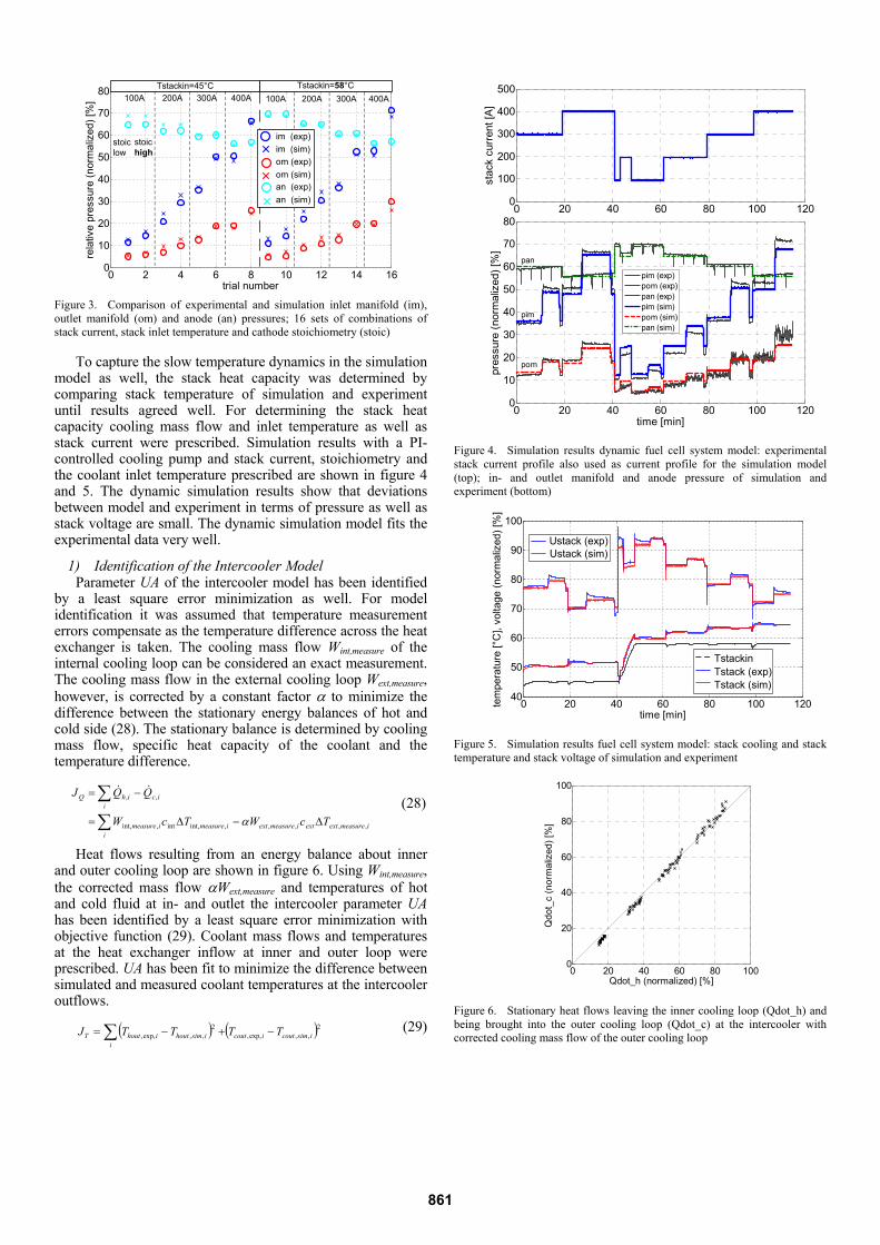
To capture the slow temperature dynamics in the simulation model as well, the stack heat capacity was determined by comparing stack temperature of simulation and experiment until results agreed well. For determining the stack heat capacity cooling mass flow and inlet temperature as well as stack current were prescribed. Simulation results with a PI-controlled cooling pump and stack current, stoichiometry and the coolant inlet temperature prescribed are shown in figure 4 and 5. The dynamic simulation results show that deviations between model and experiment in terms of pressure as well as stack voltage are small. The dynamic simulation model fits the experimental data very well.

1) Identification of the Intercooler Model Parameter UA of the intercooler model has been identified

by a least square error minimization as well. For model identification it was assumed that temperature measurement errors compensate as the temperature difference across the heat exchanger is taken. The cooling mass flow Wint,measure of the internal cooling loop can be considered an exact measurement. The cooling mass flow in the external cooling loop Wext,measure, however, is corrected by a constant factor α to minimize the difference between the stationary energy balances of hot and cold side (28). The stationary balance is determined by cooling mass flow, specific heat capacity of the coolant and the temperature difference.

∑∑

Δ−Δ=

−=

iimeasureextextimeasureextimeasureimeasure

iicihQ

TcWTcW

QQJ

,,,,,int,int,int,

,,

α (28)

Heat flows resulting from an energy balance about inner and outer cooling loop are shown in figure 6. Using Wint,measure, the corrected mass flow αWext,measure and temperatures of hot and cold fluid at in- and outlet the intercooler parameter UA has been identified by a least square error minimization with objective function (29). Coolant mass flows and temperatures at the heat exchanger inflow at inner and outer loop were prescribed. UA has been fit to minimize the difference between simulated and measured coolant temperatures at the intercooler outflows.

( ) ( 2,,exp,,

2,,exp,, isimcouticout

iisimhoutihoutT TTTTJ −+−= ∑ ) (29)

0 20 40 60 80 100 1200

100

200

300

400

500

stac

k cu

rren

t [A]

0 20 40 60 80 100 1200

10

20

30

40

50

60

70

80

pim

pom

pan

time [min]

pres

sure

(nor

mal

ized

) [%

]

pim (exp)pom (exp)pan (exp)pim (sim)pom (sim)pan (sim)

Figure 4. Simulation results dynamic fuel cell system model: experimental stack current profile also used as current profile for the simulation model (top); in- and outlet manifold and anode pressure of simulation and experiment (bottom)

0 20 40 60 80 100 12040

50

60

70

80

90

100

time [min]

tem

pera

ture

[°C

], vo

ltage

(nor

mal

ized

) [%

]

Ustack (exp)Ustack (sim)

TstackinTstack (exp)Tstack (sim)

Figure 5. Simulation results fuel cell system model: stack cooling and stack temperature and stack voltage of simulation and experiment

0 20 40 60 80 1000

20

40

60

80

100

Qdot_h (normalized) [%]

Qdo

t_c

(nor

mal

ized

) [%

]

Figure 6. Stationary heat flows leaving the inner cooling loop (Qdot_h) and being brought into the outer cooling loop (Qdot_c) at the intercooler with corrected cooling mass flow of the outer cooling loop

861

A comparison of simulation results and experimental data for different sets of stack current, outer loop cooling temperature and cooling mass flow are shown in figure 5. An increase of stack current leads to an increase of coolant temperature in the inner loop as the thermal load is increased which can be seen by the polarization curve in figure 2.

0 20 40 60 80 10050

60

70

80

90

100

trial

tem

pera

ture

(nor

mal

ilzed

) [%

]

400A100A 200A 300A

TICinincreasing

Wextincreasing

Thout (exp)Thout (sim)Tcout (exp)Tcout (sim)

45 50 55 60 65 70 75 80 85 90 9550

60

70

80

90

100

Wext =18.75%

Wext

=25%

Wext =31.25%

Wext

=37.5%

Wext =43.75%

Wext =50%

mass flow (inner loop, normalized) [%]

effe

ctiv

enes

s [%

]

Figure 7. Comparison of experimental and simulation model outlet temperature of inner (Thout) and outer (Tcout) cooling loop; for different sets of stack current, outer loop cooling temperature TICin and outer loop cooling mass flow Wext; cathode stoichiometry was kept constant (top); effectiveness of the intercooler model for all experimental trials and shown for various cooling mass flows in the inner and outer loop (bottom)

As shown in figure 7 the intercooler simulation results of the stationary model fit the experimental data very well. Furthermore, the heat exchanger effectiveness changes significantly within an interval of 50-95%. Figure 7 also shows the evolution of the effectiveness for constant mass flows Wext in the outer loop while the flow in the inner loop Wint is varied. For constant Wext the effectiveness could be approximated by a constant, however still can change significantly depending on the choice of Wext. As future controller designs possibly work with various pump speeds, a simulation model that is correct over the whole operating range of the fuel cell system is necessary. Therefore, the effectiveness is modeled as in [10] being dependent on cooling mass flows. For the dynamic simulation model parameters such as manifold, cathode and anode volumes and pipe coolant masses were determined by the system geometry and data provided by the manufacturer.

IV. COOLING CONTROLLER ARCHITECTURE For the design of a stack inlet cooling temperature control

the fuel cell system is considered a stack current dependent heat source generating a heat flow into the inner cooling loop as shown in figure 1. Evaluating the cooling system model at steady state and neglecting the hydrogen compressor’s influence, the steady state valve position uss to reach a certain stack inlet temperature Tstackin,ref can be obtained by (30) with the cooler temperate Tcooler.

⎟⎟⎠

⎞⎜⎜⎝

⎛−++−

=

coolerrefstackinc

FCFC

h

FCc

FCss

TTC

QCQ

CQ

C

Qu

,minε

(30)

An estimation of the thermal load is obtained by (31) with the actual electrical power Pstack = Ustack Istack and a cell voltage corresponding to the lower heating value (LHV) of hydrogen as the stack is partly cooled by evaporation of product water in the cathode. The cooler temperature Tcooler is being measured. The heat exchanger effectiveness ε and heat capacity flows Ch, Cc and Cmin are obtained by (25)-(26) using the measured cooling mass flows Wint and WextIC.

stackstackcellsLHVFC PInUQ −= (31)

The control law proposed is a combination of the nonlinear feedforward control and a linear proportional and integral controller with an anti-windup to prevent integrator windup (32). The anti-windup circuit is active for controller outputs greater than 100% (awindup =100%-u) and outputs less than 0% (awindup = 0%-u) and is inactive otherwise (awindup=0). The controller gains kp >0 and ki >0 add with a negative sign as shown in (32) as the cooling valve needs to open for negative control errors (Tstackin > Tstackin,ref) and to close for positive ones.

( ) ∫ −−−−−= dtaTTkTTkuu windupstackinrefstackinistackinref

stackinpss , (32)

A constant cooling mass flow Wext in the outer loop is set for the controller. Increasing the cooling mass flow would improve the cooling system dynamics as states in (21). Higher mass flows reduce the time constants for temperature in the pipe volumes. Higher pump speeds, however, result in higher power consumption. Nevertheless, the stack temperature can be set by either actuating the cooling valve or actuating the pump within certain limits set by the intercooler. This circumstance can be exploited for future control designs such that an optimal balance between pump and valve is found to optimize for power consumption or time. Here, the cooling mass flow Wext is set constant.

V. SIMULATION RESULTS The simulation model is developed and run in

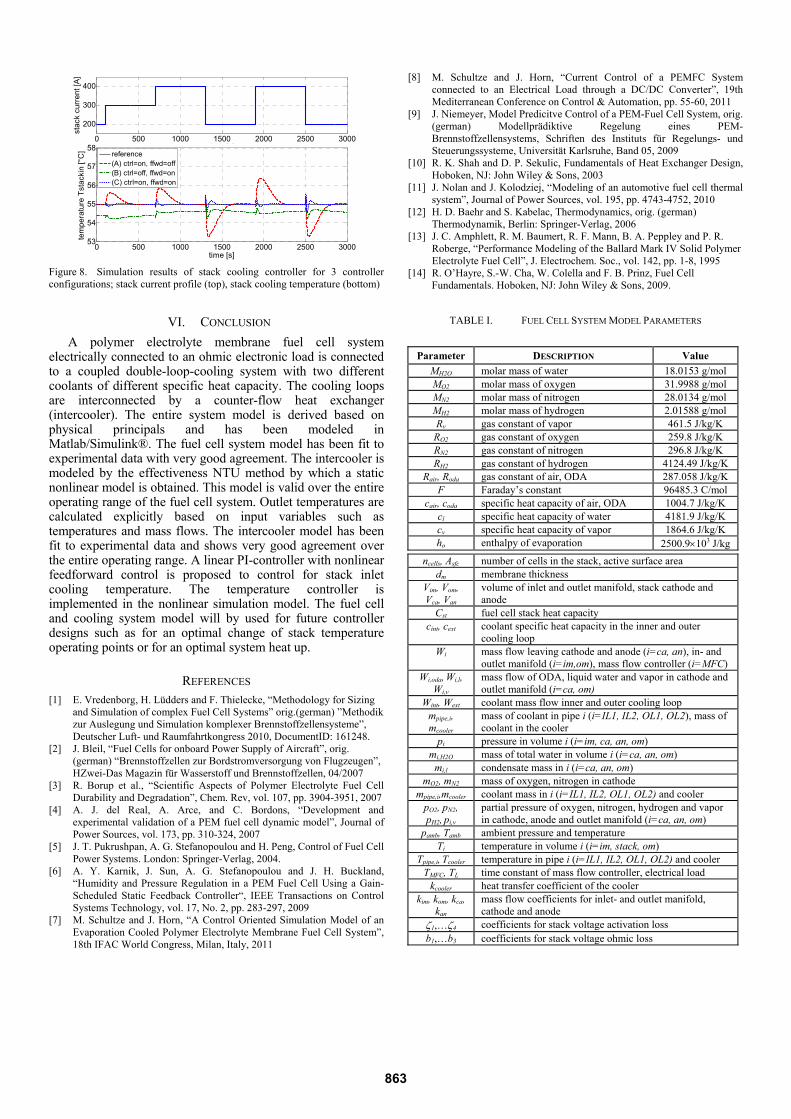
Matlab/Simulink®. The controller for stack inlet cooling temperature is connected with the nonlinear fuel cell system model. The simulation was run for a stack cooling reference temperature of 55°C and high cathode stoichiometry. Figure 8 shows the simulation results of three controller variants:

(A) PI-control activated, feedforward control deactivated (B) PI-control deactivated and feedforward control activated (C) PI- and feedforward control activated.

For a constant stack cooling reference temperature of 55°C a stack current profile as shown in figure 8 was taken to test the controller for different thermal loads. With a pure feedforward control (type B) stack temperature in steady state is close to the reference temperature. The control behavior is further improved by a linear PI-controller (type C). The temperature matches the reference in steady state and under- as well as overshoots are less than in the case of a linear controller without feedforward control (type A).

862

0 500 1000 1500 2000 2500 3000

200

300

400

i [ ]

stac

k cu

rren

t [A]

0 500 1000 1500 2000 2500 300053

54

55

56

57

58

time [s]

tem

pera

ture

Tst

acki

n [°

C]

reference(A) ctrl=on, ffwd=off(B) ctrl=off, ffwd=on(C) ctrl=on, ffwd=on

Figure 8. Simulation results of stack cooling controller for 3 controller configurations; stack current profile (top), stack cooling temperature (bottom)

VI. CONCLUSION A polymer electrolyte membrane fuel cell system

electrically connected to an ohmic electronic load is connected to a coupled double-loop-cooling system with two different coolants of different specific heat capacity. The cooling loops are interconnected by a counter-flow heat exchanger (intercooler). The entire system model is derived based on physical principals and has been modeled in Matlab/Simulink®. The fuel cell system model has been fit to experimental data with very good agreement. The intercooler is modeled by the effectiveness NTU method by which a static nonlinear model is obtained. This model is valid over the entire operating range of the fuel cell system. Outlet temperatures are calculated explicitly based on input variables such as temperatures and mass flows. The intercooler model has been fit to experimental data and shows very good agreement over the entire operating range. A linear PI-controller with nonlinear feedforward control is proposed to control for stack inlet cooling temperature. The temperature controller is implemented in the nonlinear simulation model. The fuel cell and cooling system model will by used for future controller designs such as for an optimal change of stack temperature operating points or for an optimal system heat up.

REFERENCES [1] E. Vredenborg, H. Lüdders and F. Thielecke, “Methodology for Sizing

and Simulation of complex Fuel Cell Systems” orig.(german) ”Methodik zur Auslegung und Simulation komplexer Brennstoffzellensysteme”, Deutscher Luft- und Raumfahrtkongress 2010, DocumentID: 161248.

[2] J. Bleil, “Fuel Cells for onboard Power Supply of Aircraft”, orig. (german) “Brennstoffzellen zur Bordstromversorgung von Flugzeugen”, HZwei-Das Magazin für Wasserstoff und Brennstoffzellen, 04/2007

[3] R. Borup et al., “Scientific Aspects of Polymer Electrolyte Fuel Cell Durability and Degradation”, Chem. Rev, vol. 107, pp. 3904-3951, 2007

[4] A. J. del Real, A. Arce, and C. Bordons, “Development and experimental validation of a PEM fuel cell dynamic model”, Journal of Power Sources, vol. 173, pp. 310-324, 2007

[5] J. T. Pukrushpan, A. G. Stefanopoulou and H. Peng, Control of Fuel Cell Power Systems. London: Springer-Verlag, 2004.

[6] A. Y. Karnik, J. Sun, A. G. Stefanopoulou and J. H. Buckland, “Humidity and Pressure Regulation in a PEM Fuel Cell Using a Gain-Scheduled Static Feedback Controller“, IEEE Transactions on Control Systems Technology, vol. 17, No. 2, pp. 283-297, 2009

[7] M. Schultze and J. Horn, “A Control Oriented Simulation Model of an Evaporation Cooled Polymer Electrolyte Membrane Fuel Cell System”, 18th IFAC World Congress, Milan, Italy, 2011

[8] M. Schultze and J. Horn, “Current Control of a PEMFC System connected to an Electrical Load through a DC/DC Converter”, 19th Mediterranean Conference on Control & Automation, pp. 55-60, 2011

[9] J. Niemeyer, Model Predicitve Control of a PEM-Fuel Cell System, orig. (german) Modellprädiktive Regelung eines PEM-Brennstoffzellensystems, Schriften des Instituts für Regelungs- und Steuerungssysteme, Universität Karlsruhe, Band 05, 2009

[10] R. K. Shah and D. P. Sekulic, Fundamentals of Heat Exchanger Design, Hoboken, NJ: John Wiley & Sons, 2003

[11] J. Nolan and J. Kolodziej, “Modeling of an automotive fuel cell thermal system”, Journal of Power Sources, vol. 195, pp. 4743-4752, 2010

[12] H. D. Baehr and S. Kabelac, Thermodynamics, orig. (german) Thermodynamik, Berlin: Springer-Verlag, 2006

[13] J. C. Amphlett, R. M. Baumert, R. F. Mann, B. A. Peppley and P. R. Roberge, “Performance Modeling of the Ballard Mark IV Solid Polymer Electrolyte Fuel Cell”, J. Electrochem. Soc., vol. 142, pp. 1-8, 1995

[14] R. O’Hayre, S.-W. Cha, W. Colella and F. B. Prinz, Fuel Cell Fundamentals. Hoboken, NJ: John Wiley & Sons, 2009.

TABLE I. FUEL CELL SYSTEM MODEL PARAMETERS

Parameter DESCRIPTION Value MH2O molar mass of water 18.0153 g/mol MO2 molar mass of oxygen 31.9988 g/mol

MN2 molar mass of nitrogen 28.0134 g/mol MH2 molar mass of hydrogen 2.01588 g/mol Rv gas constant of vapor 461.5 J/kg/K RO2 gas constant of oxygen 259.8 J/kg/K RN2 gas constant of nitrogen 296.8 J/kg/K RH2 gas constant of hydrogen 4124.49 J/kg/K

Rair, Roda gas constant of air, ODA 287.058 J/kg/K F Faraday’s constant 96485.3 C/mol

cair, coda specific heat capacity of air, ODA 1004.7 J/kg/K cl specific heat capacity of water 4181.9 J/kg/K cv specific heat capacity of vapor 1864.6 J/kg/K ho enthalpy of evaporation 2500.9×103 J/kg

ncells, Asfc number of cells in the stack, active surface area dm membrane thickness

Vim, Vom, Vca, Van

volume of inlet and outlet manifold, stack cathode and anode

Cst fuel cell stack heat capacity cint, cext coolant specific heat capacity in the inner and outer

cooling loop Wi mass flow leaving cathode and anode (i=ca, an), in- and

outlet manifold (i=im,om), mass flow controller (i=MFC) Wi,oda, Wi,l,

Wi,v mass flow of ODA, liquid water and vapor in cathode and outlet manifold (i=ca, om)

Wint, Wext coolant mass flow inner and outer cooling loop mpipe,i, mcooler

mass of coolant in pipe i (i=IL1, IL2, OL1, OL2), mass of coolant in the cooler

pi pressure in volume i (i=im, ca, an, om) mi,H2O mass of total water in volume i (i=ca, an, om)

mi,l condensate mass in i (i=ca, an, om) mO2, mN2 mass of oxygen, nitrogen in cathode

mpipe,i,mcooler coolant mass in i (i=IL1, IL2, OL1, OL2) and cooler pO2, pN2, pH2, pi,v

partial pressure of oxygen, nitrogen, hydrogen and vapor in cathode, anode and outlet manifold (i=ca, an, om)

pamb, Tamb ambient pressure and temperature Ti temperature in volume i (i=im, stack, om)

Tpipe,i, Tcooler temperature in pipe i (i=IL1, IL2, OL1, OL2) and cooler TMFC, TL time constant of mass flow controller, electrical load

kcooler heat transfer coefficient of the cooler kim, kom, kca,

kan mass flow coefficients for inlet- and outlet manifold, cathode and anode

ζ1,…ζ4 coefficients for stack voltage activation loss b1,…b3 coefficients for stack voltage ohmic loss

863