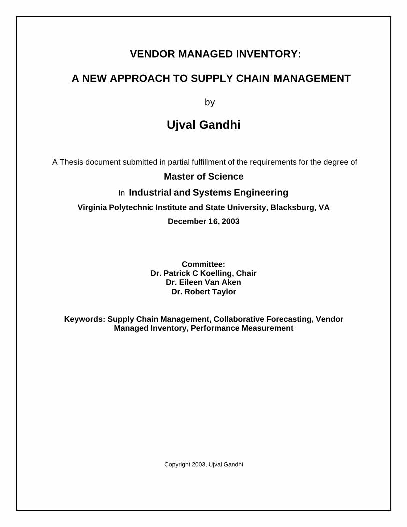
VENDOR MANAGED INVENTORY:

A NEW APPROACH TO SUPPLY CHAIN MANAGEMENT

by

Ujval Gandhi A Thesis document submitted in partial fulfillment of the requirements for the degree of

Master of Science

In Industrial and Systems Engineering

Virginia Polytechnic Institute and State University, Blacksburg, VA

December 16, 2003

Committee: Dr. Patrick C Koelling, Chair

Dr. Eileen Van Aken Dr. Robert Taylor

Keywords: Supply Chain Management, Collaborative Forecasting, Vendor Managed Inventory, Performance Measurement

Copyright 2003, Ujval Gandhi

Vendor Managed Inventory: A new approach to supply chain

management

Ujval Gandhi

ABSTRACT

The Global Supply Chain Forum (Stanford Global Supply Chain Forum

Web Resource, http://www.stanford.edu/groups/scforum) defines supply

chain management (SCM) as

“Supply chain management is the integration of key business processes from

end user through original suppliers that provides products, services and

information that add value for customer and other stakeholders”

The rapid development of the Internet has dramatically changed the

traditional definitions of manufacturer, suppliers and customers. Newer

approaches to supply chain management attempt to organize the supply

chain as a network of cooperating intelligent agents, each performing one or

more supply chain functions and each coordinating actions with one another.

This research is aimed at creating a viable model of a single manufacturer-

single supplier collaborative supply chain system using a Vendor Managed

Inventory (VMI) system. The research further uses known inventory

performance parameters to performance benchmark the VMI system with

traditional push-pull systems, develop a collaborative forecasting

spreadsheet solution and a best alternative ordering policy amongst EOQ,

Monthly, JIT and VMI policies under known lead time and a variety of

demand distribution functions.

iii

ACKNOWLEDGMENTS My sincerest thanks to Dr. Patrick Koelling for his guidance and helping

me carry out this research. The undertaking and completion of my thesis

would have been impossible without his guidance and support. I greatly

appreciate the contributions of the other committee members, Dr. Eileen

Van Aken and Dr. Robert Taylor.

I dedicate this work to my family. My mother and father, Varsha and

Sudhir Gandhi, my brother Dr. Umang Gandhi and his wife, Dr. Archana

Gandhi and little Mahek. Their love and constant support helped me face the

rigors of a Masters’ degree in a new surrounding.

Sincere thanks to my extended family in Blacksburg. It was great to

have Biju, Kunal, Yogesh, Chandresh, Kavita and Harish around. This thesis

would have not been possible without the extra efforts and constant

encouragement by Amar, who took great pains to explain to me what

actually went into database programming and Keer, who listened patiently at

whatever I threw at him. I will always be thankful to Kartik, who always

taught me, “It’s not whether you get knocked down, it’s whether you get

up”. Smruti deserves a special thanks for all the hard work she put in

plotting my flowcharts, going through my presentation slides and providing

me constant encouragement, listening to my constant bickering, making me

always feel welcome and having a smile for everyone around. It was great to

have everyone around!

Last but not the least, I would also like to extend my sincere thanks to

Ms. Lovedia Cole, the graduate secretary of the department. She has been

extremely helpful ever since the day I arrived here.

iv

TABLE OF CONTENTS No Topic Page

1 INTRODUCTION 1

1.1 GLOBALIZATION AND CHALLENGES 1

1.2 SUPPLY CHAIN CONSTITUENTS 2

1.3 PROBLEM STATEMENT 4

1.4 RESEARCH OBJECTIVES 5

1.5 RESEARCH METHODOLOGY 5

2 VENDOR MANAGED INVENTORY (VMI) SYSTEMS 8

2.1 INTRODUCTION 8

2.2 VMI PROGRAMS 9

2.3 VMI BENEFITS 10

2.4 VMI PROCESS DESCRIPTION 12

2.5 SUPPLY CHAIN MODEL FOR VMI 14

2.6 STOCK REPLENISHMENT AND SHIPMENT

SCHEDULING IN VMI SYSTEMS 19

2.7 VMI SOFTWARE DEMONSTRATION 20

2.7.1 FLOW-CHARTING PROCESS 21

2.7.2 TABLE RELATIONSHIPS 26

2.7.3 APPLICATION SYSTEM SNAP-SHOTS 28

3 POLICY COMPARISONS 31

3.1 ORDERING POLICIES 31

3.1.1 ECONOMIC ORDER QUANTITY 31

3.1.2 MONTHLY POLICY 32

3.1.3 JUST IN TIME POLICY 32

3.1.4 VENDOR MANAGED INVENTORY POLICY 32

3.2 BASIC DEMAND DATA 32

v

3.2.1 UNIFORM DISTRIBUTION 34

3.2.2 TRIANGULAR DISTRIBUTION 34

3.2.3 POISSON DISTRIBUTION 35

3.3 SYSTEM PARAMETERS 35

3.3.1 INDEPENDENT VARIABLES 35

3.3.2 SYSTEM CONSTANTS 35

3.3.3 DEPENDENT VARIABLES 36

3.4 EXPERIMENTAL ANALYSIS 38

3.5 EXPERIMENTAL RESULTS 41

3.5.1 UNIFORM DISTRIBUTION 41

3.5.2 TRIANGULAR DISTRIBUTION 42

3.5.3 POISSON DISTRIBUTION 43

3.6 COMPARATIVE RESULTS 44

3.6.1 EOQ BASED POLICIES 44

3.6.2 TOTAL COSTS COMPARISON ACROSS THE THREE DEMAND DISTRIBUTION FUNCTION

45

3.6.3 AVERAGE DAILY INVENTORY COMPARISON ACROSS THE THREE DEMAND DISTRIBUTION FUNCTIONS

47

3.6.4 INVENTORY TURNS COMPARISON ACROSS THE THREE DEMAND DISTRIBUTION FUNCTIONS 49

3.6.5 FULFILLMENT RATE COMPARISON ACROSS THE THREE DEMAND DISTRIBUTION FUNCTIONS 51

3.6.6 SERVICE EFFICIENCY LEVEL COMPARISON ACROSS THE THREE DEMAND DISTRIBUTION FUNCTIONS 53

3.7 DEVELOPMENT OF A BEST ALTERNATIVE ORDERING POLICY

57

3.7.1 SINGLE SUPPLIER STRATEGY 58

3.7.2 CHANGE IN SHIPMENT POLICIES 58

3.7.3 INVENTORY RE-ROUTING 63

vi

4 CONCLUSIONS 66

4.1 SUMMARY 66

4.2 FINDINGS FROM THE CURRENT DATA 66

4.3 SUPPLY CHAIN OF THE FUTURE 67

4.4 FURTHER DIRECTIONS OF RESEARCH 69

APPENDIX 73

A UNIFORM DISTRIBUTION 73

B TRIANGULAR DISTRIBUTION 74

C POISSON DISTRIBUTION 75

vii

LIST OF FIGURES Figure 1.1 Flows within a supply chain 2

Figure 1.2 Research Methodology 7

Figure 2.1 Typical VMI Setup Program 13

Figure 2.2 VMI Process Flowchart - 1 22

Figure 2.3 VMI Process Flowchart – 2 23

Figure 2.4 VMI Process Flowchart – 3 24

Figure 2.5 Table relationships in the application system 27

Figure 2.6 Customer Menu Login Page 28

Figure 2.7 Supplier Menu Login Page 29

Figure 2.8 Manufacturer Menu Login Page 30

Figure 3.1 Monthly Demand Function – Uniform Distribution 34

Figure 3.2 Monthly Demand Function – Triangular Distribution 34

Figure 3.3 Monthly Demand Function – Poisson Distribution 35

Figure 3.4 Total Costs Comparison – Four ordering policies for Uniform distribution

45

Figure 3.5 Total Costs Comparison – Four ordering policies for Triangular distribution

46

Figure 3.6 Total Costs Comparison – Four ordering policies for Poisson Distribution

47

Figure 3.7 Average Daily Inventory – Uniform Distribution 48

Figure 3.8 Average Daily Inventory – Triangular Distribution 48

Figure 3.9 Average Daily Inventory – Poisson Distribution 49

Figure 3.10 Inventory Turns Comparison – Uniform Distribution 50

Figure 3.11 Inventory Turns Comparison – Triangular Distribution 50

Figure 3.12 Inventory Turns Comparison – Poisson Distribution 51

Figure 3.13 Fulfillment Rate Comparison – Uniform Distribution 52

Figure 3.14 Fulfillment Rate Comparison – Triangular Distribution 52

Figure 3.15 Fulfillment Rate Comparison – Poisson Distribution 53

Figure 3.16 Service Efficiency Level Comparison – Uniform Distribution 54

Figure 3.17 Service Efficiency Level Comparison – Triangular Distribution

55

viii

Figure 3.18 Service Efficiency Level Comparison – Poisson Distribution 55

Figure 3.19 Comparison of Average Inventory and Service Efficiency – Uniform Distribution

56

Figure 3.20 Comparison of Average Inventory and Service Efficiency – Triangular Distribution

56

Figure 3.21 Comparison of Average Inventory and Service Efficiency – Poisson Distribution

57

Figure 3.22 Variation in shipment quantities for the JIT policy 59

Figure 3.23 Units/Shipment in a JIT ordering policy 60

Figure 3.24 Comparison of VMI and JIT shipment quantities 61

Figure 3.25 Comparison of number of shipments – JIT and VMI 61

Figure 3.26 Differences in using FTL and LTL shipment modes for the JIT ordering policy 62

Figure 3.27 Transportation capacity utilization comparison 63

Figure 3.28 Average Inventory Comparison – JIT and VMI 64

Figure 3.29 Comparison between service efficiency levels 65

ix

LIST OF TABLES Table 3.1 Demand Data 33

Table 3.2 System Summary 38

Table 3.3 Inventory Availability Calculation 39

Table 3.4 System Summary – Uniform Distribution Dataset 1 41

Table 3.5 System Summary – Uniform Distribution Dataset 2 41

Table 3.6 System Summary – Triangular Distribution Dataset 1 42

Table 3.7 System Summary – Triangular Distribution Dataset 2 42

Table 3.8 System Summary – Poisson Distribution Dataset 1 43

Table 3.9 System Summary – Poisson Distribution Dataset 2 43

Table 3.10 Coefficient of variation comparison 44

Table 3.11 Comparative Analysis – Service Efficiency and Average Inventory carried 54

1

CHAPTER 1. INTRODUCTION

1.1 GLOBALIZATION AND CHALLENGES

Market globalization has forced enterprises to rethink traditional supply

chain approaches. With the development of the Internet, customers are no

longer restricted to local buying. Companies must increasingly focus on

gaining competitive advantage through effective management of their supply

chains. The e-business revolution is affecting supply chain management

dramatically and is changing how companies integrate business processes,

both inside and outside the enterprise. These developments introduce new

business and technical challenges and spotlight existing business processes

and supporting enterprise systems that revolve around the supply chain.

Newer approaches to supply chain management attempt to organize the

supply chain as a network of cooperating intelligent agents, each performing

one or more supply chain functions and each coordinating action with one

another (Horvath, 2001).

The common characteristic among supply chain leaders in all the

industry segments is the extent to which the various supply chain

constituents engage in supply chain collaboration. Organizations need to

break the traditional paradigm of looking at the supply chain as a set of

inter-connected constituents (Sahay, 2003). There is an urgent need to

employ systems thinking to supply chain management.

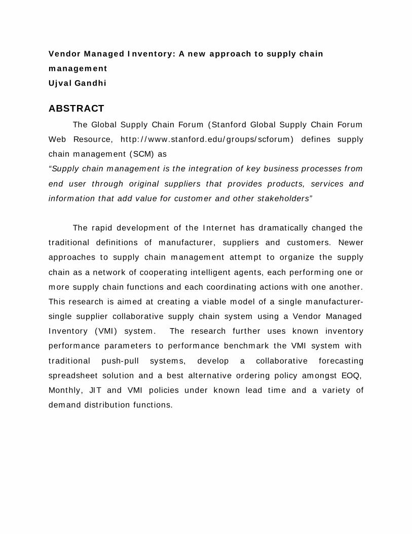
1.2 SUPPLY CHAIN CONSTITUENTS Figure 1.1 illustrates the physical movement of products through a

supply chain network for a manufactured product. The flow begins with

several suppliers. They send raw materials/components to a factory. The

factory either manufactures products or assembles them and sends the

2

finished products to regional warehouses or to distribution centers. The

warehouses and distribution centers support the customers.

Figure 1.1 Flows within a supply chain

A typical supply chain is comprised of a manufacturer, one or more

suppliers, distribution centers and retailer owned warehouses all serving the

various downstream customers. Traditionally, the focus of companies has

been on the flows within the organization or the flows over which the

organization has direct control (Sahay, 2003). Supply chain management

has done a very effective job of optimizing the individual supply chain

constituents. However, successful supply chain management requires the

recognition that the firm is simply one player in the long chain that starts

with the suppliers and includes transporters, distributors and customers

(Sahay, 2003). Organizations must interact cooperatively with their channel

partners (e.g. suppliers, distribution centers, etc.) for the mutual benefit of

the channel as well as the gain of each player. In order to adopt this

systems perspective, organizations should not only consider the impact of

any business decision on their own performance but also on the bottom line

of their suppliers, distributors and transporters. Anderson and Lee (1999)

call the new generation of supply chain strategy a “synchronized supply

chain.”

As organizations enter the era of network competition, the winners will

be those organizations that can better structure, coordinate and manage the

relationships with their partners in a network committed to better, faster and

Suppliers Customers Factory

Distribution Centers

Warehouses

3

closer relationships with their final customers (Christopher, 1999). As

organizations look beyond their own firms, it becomes important for them to

involve their suppliers and customers in the various processes. Successful

involvement yields major benefits: increased market share, inventory

reductions, improved delivery service, improved quality and shorter product

development cycles (Corbett et. al., 1999).

1.3 PROBLEM STATEMENT

Given the challenges posed by market globalization, there is a pressing

need for newer approaches to supply chain management. Systems

increasingly reflect supply chain costs from an integrated picture.

Collaborative supply chain planning (CSCP) not only respects constraints, it

reflects cost and profit objectives.

One of the important issues to be addressed in the development of a

collaborative supply chain is the ordering and replenishment policy to be

followed. An ordering policy that does not adhere to the principles of

collaborative supply chain management can translate to sub-optimization in

supply chains and, consequently, enormous losses for the organization

(Sahay, 2002). One example of a CSCP system is Vendor Managed

Inventory (VMI). Unlike a traditional business model which orders on the

basis of an ordering amount decided by commonly known formulae like EOQ,

in a VMI system, the supplier receives electronic data (usually through an

Electronic Data Exchange or the Internet) that informs him about the

manufacturer’s sales and stock levels. The supplier is responsible for

creating and managing the inventory replenishment schedule.

4

The research questions to be addressed in this thesis are:

Given the necessity for a collaborative supply chain

environment in the current market scenario, what are the functional

requirements for the development of a single-echelon system

incorporating VMI principles under known lead-time and variable

demand? How does a VMI ordering policy compare against standard

ordering policies incorporating Economic Order Quantity, Monthly

ordering and Just in time ordering on the basis of known inventory

measures and under a variety of demand distribution functions?

Additionally, can a spreadsheet analysis provide the best alternative

among the four ordering policies mentioned?

1.4 RESEARCH OBJECTIVES

Horvath (2001) and Sahay (2002) identified the necessity for a

collaborative supply chain environment as being essential to the success of

any organization in the current paradigm of globalization. This research will

require the development of an ordering policy for single manufacturer-single

supplier supply chains with known lead-time and variable demand.

Additionally, a collaborative supply chain model will be constructed that can

serve as a building block for quantifying the inventory and service

performance of supply chains in dynamic settings. The research question will

be answered by constructing a database application system incorporating

VMI logic. Using the results from the database system and a systems

dynamics model, a best alternative ordering policy for a single

manufacturer-single supplier system can be developed by a statistical

analysis of four ordering policies – EOQ, Monthly, JIT and VMI-under three

demand distribution functions – Uniform, Triangular and Poisson.

5

1.5 RESEARCH METHODOLOGY

The research method will be accomplished in three distinct phases.

Each phase is incremental in nature and can generally be described by the

primary steps that will occur in each – they are the modeling phase, the

application system development phase, and the analysis phase.

The modeling phase consists of analyzing the supply chain constituents

to create a conceptual design of a VMI network. With global competition

imposing tremendous pressure on product and service providers to

transform and improve their operations and practices, firms are

reconsidering the design of traditional Supply Chain Networks (SCN) as a

solution for effectively meeting customer requirements such as low costs,

high product variety and short lead times (Crainic, 2000). The modeling

phase will integrate the Axsater (2002) model, which will be used to

investigate stock replenishment and shipment scheduling in VMI systems.

The application system design phase consists of the design and

development of a database system incorporating VMI principles. The

application system is limited to the design and implementation for a single

manufacturer-single supplier-single distribution center system. Systems

incorporating multi-echelon supply chain constituents will not be considered

in this research. The application system for the MRP system will incorporate

three ordering policies – EOQ, Monthly ordering policy and JIT ordering

policy-under three demand distribution patterns – Uniform, Triangular and

Poisson. The time period under review is one fiscal year, operating from

January 1 to December 31. The system will incorporate C code that will write

output results to a text file for analysis.

The analysis phase involves using the results of Kaplan and Norton

(1996) and Beamon (2000) to generate a list of performance measures.

These performance measures will be concentrated in the process metrics

category with special emphasis on inventory management. Microsoft Excel

6

will be used to generate performance curves based on inventory measures

and creation of two-axis graphs for policy comparisons under the different

demand distributions.

The research methodology can be represented in a flowchart

representation as illustrated in Figure 1.2.

7

Figure 1.2 Research Methodology

Identify supply chain constituents

Spreadsheet solution for

collaborative forecasting

Establish criteria for SCN design

Establish system

parameters

Integrate the Axsater

model for VMI system in the SCN

Test the model

parameters by a dry

run

Test results

MODELING

Core model

Follow data

hierarchy

Develop metrics

Structure output (data)

files

Run scenarios

Create backend of database

APPLICATION SYSTEM DEVELOPMENT

System queries to provide output results for VMI ordering policy; Use as input for creating Excel

Spreadsheet incorporating three more ordering policies – EOQ, Monthly and JIT - under three

demand distributions – Uniform, Triangular and Poisson.

Generate performance curves based on inventory

measures

Create 2-axis graphs for policy

comparisons

Perform sensitivity analysis

End

ANALYSIS

Iterative Design for front end and system functionality

Develop recommendations based on analysis and derive a best

alternative ordering policy

8

CHAPTER 2. VENDOR MANAGED INVENTORY (VMI)

SYSTEMS

2.1 INTRODUCTION

Hall (1998) defines VMI as a process where the supplier generates

orders for the customers based on demand information sent by the

customer.

One of the most challenging issues for fulfilling customer needs is to

manage the order delivery process between the various supply chain

constituents (Kaipia, 2002). One of the primary goals of effective supply

chain management is to develop processes between all the supply chain

members that minimize the wastage of time and enable fast and reliable

reactions to demand changes. A traditional order delivery process is based

on the principle that the manufacturer/retailer defines the amount and

timing of deliveries of each item needed from the supplier. The supplier’s

task is to fulfill this as closely as possible. Exactly how this is done varies,

depending on the industry and the company. Retailing organizations place

purchase orders for every delivery, whereas manufacturing industries use

economic order quantity purchases (Kaipia, 2002).

Fast transfer of information between organizations has, since the

introduction of electronic data interchanges (EDI), been considered a key

issue in improving the performance of supply chains. Just-in-time and agile

practices like smaller lot sizes and frequent deliveries have been applied to

permit the suppliers to react faster to changes in the customer’s demand.

However, there are several serious problems with the demand fulfillment

solution using traditional approaches.

• The actual item level replenishment cycle is far slower than the order

fulfillment cycle. A survey of manufacturers and retailers in United States

9

(Horvath, 2001) illustrates that frequently an order was placed when the

product was already sold out or so late that the product would be out of

stock before the delivery arrives.

• On the supplier side, there are high levels of inventory because of the

short delivery time and high service level requirements. Typically, there

exists accurate information neither about retail sales nor about out-of-

stocks along the chain. This means that the real trade-off between

providing a good logistics service level and cost level remains hidden from

the supplier. Lee, et. al (1997) illustrated the development of the bullwhip

effect in both manufacturing and retail scenarios using this fact.

2.2 VENDOR MANAGED INVENTORY PROGRAMS

Vendor Managed Inventory, VMI, is an alternative for the traditional order

based replenishment practices. VMI is a fundamental change in the approach

for solving the problem of supply chain coordination. Instead of putting more

pressure on suppliers performance by requiring faster and more accurate

deliveries, VMI gives the supplier both responsibility and authority to

manage the entire replenishment process. The manufacturer/retailer

provides the supplier access to inventory and demand information and sets

the targets for availability. Thereafter, the supplier decides when and how

much to deliver. The measure for the supplier’s performance is availability

and inventory turnover. This is a fundamental change that affects the

operational mode both at the customer and at the supplier company. Waller

(1999) investigated the impacts of VMI through simulation. The study shows

how replacing purchase orders with inventory replenishments enable

suppliers to improve service while reducing supply chain costs. The reason

for this is that in VMI the inventory of the average product is reviewed more

frequently than purchase orders were placed before. For the average item,

the more frequent review in the VMI approach reduces the ordering delay in

10

the information flow. Other VMI benefits (Cottrill, 1997, Nolan, 1998) are

more long term in nature. The introduction of VMI gives the supplier more

time to react - i.e. it levels demand and in this way brings benefits in

reduced inventories and in effective production planning and control.

It is important to note that the more frequent inventory reviews in VMI

do not require more frequent deliveries. It is exactly this requirement for

frequent deliveries that has in many cases caused problems for suppliers

when the customer has introduced the just-in-time (JIT) concept (Kaipia,

2001).

There are numerous case examples of successful VMI implementations

(Cooke, 1998, Holmstrom, 1998). However, VMI has not become a standard

way of managing replenishment processes in the supply chain. There seem

to be some practical issues that slow down the implementation of VMI in

many companies. The requirement of standard product identification and

integrated information systems in the supply chain is one example. The two

parties may also be unwilling to share information, and lack of trust often

exists (Fraza, 1998). Purchasing, and not sourcing, is seen as a core

competency of the company (Cooke, 1998). The lack of trust between the

trading partners and the uncertainty about the potential benefits of VMI are

difficult obstacles. For establishing trust a company should be able to

demonstrate to the trading partner the benefits of shifting to VMI. Also, VMI

is not a standard solution for all replenishment processes. The benefits of

VMI vary in different supply chains and according to product demand.

2.3 VMI BENEFITS (Adapted from Hall, 1998)

The main benefits of VMI are given below.

1. Lower customer Inventories is the primary benefit of a VMI

implementation program. Under VMI, the supplier is able to control the

lead time component of the order point better than a

11

manufacture/supplier with a host of suppliers can ever hope to.

Additionally, with frequent inventory review, the need for safety stocks on

the supplier side is dramatically reduced.

2. Better Forecasts occur because of demand information sharing (Cooke,

1998). Better forecasts result from having a more stable demand

distribution pattern. The demand is reflected in more frequent orders for

the same parts and therefore lower variability of demand in business.

3. Reduced costs occur because of the reduction in the demand volatility

downstream of the supply chain (Waller, 1999). VMI helps dampen the

peaks and valleys of production, allowing smaller buffers of capacity and

inventory. With VMI, greater channel coordination supports the supplier’s

need for smoother production without sacrificing the

manufacturer/retailer’s service and stock objectives (Lee, 1997).

Transportation costs are reduced with VMI because the approach helps to

increase the percentage of full truckload shipments and eliminate the

higher cost LTL shipments (Lee, 1997).

4. Improved Service. From the manufacturer/retailer’s perspective,

service is usually assessed by measuring product availability. With VMI,

coordination of replenishment orders and deliveries across multiple

suppliers helps to improve service. Lee (1997) illustrated that the adverse

effects of price markdowns and “product rollovers” can be drastically

reduced by using channel coordination programs like VMI. Finally,

coordinated logistics decisions ensure more predictable delivery schedules

in VMI systems.

12

2.4 VMI PROCESS DESCRIPTION

The Voluntary InterIndustry Commerce Standards (VICS), an umbrella

organization of industries across the United States, has defined some

common technology standards for VMI programs (VICS Web Resource,

www.vics.org).

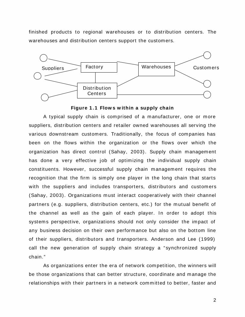
There are two EDI transactions at the heart of any VMI process.

1. Product Activity Report (852): The data contained in this document

are sales and inventory information. The inventory data are typically

segmented into various groups such as on-hand, committed, back

ordered, etc. This transaction report is the backbone of the VMI program

and is sent by the customer on a prearranged schedule, typically, on a

daily basis.

The supplier reviews the information that has been sent by the

manufacturer on the 852 to determine the necessity of an order. The

following sequence of steps is recommended by the VICS standards.

• Verification of data to ensure accuracy. Most of this verification

process is usually automated.

• On a scheduled basis, the software calculates a reorder point for

each item based on the movement data and any overrides

contributed by the manufacturer. The software compares the

quantity available at the manufacturer with the reorder point for

each item at each location. This determines the necessity of a new

order. Order generation is possible only at the manufacturer site.

• Order quantities are calculated. Order quantities also take into

account issues such as carton quantities and transact ion costs.

2. Purchase Order Acknowledgement (855): The second VMI

transaction informs the customer what product to expect from the

supplier. There are two transactions being used for this function. The

13

most frequently used is the “Purchase Order Acknowledgement”, referred

to as 855. This document contains the product numbers and quantities

ordered by the supplier on the manufacturer’s behalf. There is a feature

in the VMI software to use the 856, “Advance Ship Notice”, to alert the

manufacturer about the order and shipment. 856 differ from the 855 in

both the timing and content. The 856 is sent after the shipment has been

made instead of at the time of the order. The 856 contains only the part

numbers shipped as well as additional information such as carrier and

waybill information. The use of either the 855 or 856 is dictated by the

operational rules defined in the VMI software.

Figure 2.1 illustrates a typical VMI setup program.

Figure 2.1 Typical VMI Setup Program

EDI 850

VMI Software

EDI 855

EDI 852

Review

EDI 850

VMI Software

EDI 855

EDI 852

Review

14

2.5 A SUPPLY CHAIN MODEL FOR VMI

The model studies vendor managed inventory issues using a supply chain

model focused on inventory systems, purchase prices and purchase

quantities. The model contains two supply chain constituents;

1. a manufacturer, also referred to as buyer in supply chain terminology,

and,

2. a supplier (original equipment manufacturer or OEM in this case).

The manufacturer purchases the final product (or a major component of

it) from the OEM supplier. The manufacturer appears to be the “leader” in

this relationship, in that the manufacturer/buyer specifies order quantity

according to its own cost characteristics, and determines purchase prices for

the products provided by the supplier. However, the quantity the supplier is

willing to provide is determined by the supplier itself for a given purchase

price.

Several assumptions commonly used in inventory-channel coordination

research (Kohli and Park, 1994; Weng, 1995) are made to facilitate the

analysis of the consignment issue. Firstly, the inventory system of the

manufacturer can be described by an economic order quantity (EOQ) policy

based on deterministic demand and lead-times. The widely used EOQ policy

is considered here due to its relative robustness in a variety of situations

(Lowe and Schwarz, 1983).

Let y denote the demand per time period for the final product of the

buyer. The profit function of the buyer can be given by,

∏B = pyy – wy – (B

B

Qys

+2hB

BQ ) (i)

(Source: Kohli and Park, 1994)

where,

py is the sales price of the final product,

w is the contract purchase price determined by the buyer,

hB is the buyer’s inventory carrying cost/unit,

15

sB is the buyer’s order setup cost/unit, and

QB is the buyer’s order quantity and in this case is (2sBy/hB)1/2.

Kohli and Park (1994) showed that the buyer’s profit function is a

function of the inventory holding and ordering costs, INVB

∏B = pyy – wy – (2hBsBy)1/2 (ii)

Since the supplier takes the order quantity from the buyer as given

(QB=EOQB) and makes the necessary delivery, the supplier’s profit function,

after accounting for order setup, inventory holding and production and

delivery costs is,

∏S = wy – cy – (2

ysh BB)1/2 (

B

S

ss

+B

S

hh

) (iii)

where

cy is the production and distribution cost of the supplier,

hS represents the supplier’s carrying costs, and

sS represent the supplier’s order setup costs.

Weng (1995) and Joglekar (1998) showed that the supplier’s lot size is

treated as an integer multiple (m) of that of the buyer’s.

hS = (m-1)h’S

sS = sP + s’S/m

where,

h’S is the supplier’s actual inventory holding cost,

sP is the supplier’s fixed order processing cost per buyer’s order, and

s’S is the supplier’s setup/ordering cost per buyer’s order.

For any given purchase price w from the buyer, the supplier chooses a

quantity y to maximize its profit and it can be obtained from the first order

condition.

w = c’y + 21

(y2sh BB

)1/2(B

s

ss

+B

S

hh

) (iv)

16

The buyer can maximize its profit by choosing the optimal quantity y*, such

that:

p’y*y* + p’y* - c’y* - c”y*y* - 41

(w* - c’y*) - 21

(*ysh2 BB

)1/2 = 0. (v)

y* exists when the second order condition is satisfied and can be

solved numerically with relevant demand and cost function forms. In a

traditional setting, the buyer, using knowledge of the supplier’s cost and

willingness to supply at a given purchase price can offer the supplier a price

so as to get the optimal quantity the buyer desires.

In a VMI setting, the buyer no longer manages its inventory system

and leaves it to the supplier to determine inventory levels, order quantities,

lead times, etc. As a result, the supplier now has the combined inventory

with order setup costs (sS+sB) and carrying costs (hS+hB). The supplier’s

profit function with VMI consignment becomes

∏sc

= wcy – cy – [2(sS + sB)( hS + hB)y]1/2 (vi)

where wc represents the new pricing method the buyer uses to induce

the supplier to manage the buyer’s inventory system. In VMI terminology,

wc represents the contract purchase price. The buyer’s profit function is

∏Bc

=pyy - wcy (vii)

As the supplier maximizes its profit with the buyer’s inventory added

into the supplier’s cost and profit functions, the relationship between the

purchase price and the purchase quantity can be obtained from the first

order condition of the supplier’s profit function.

wc=c’y + 21

(c

SBSB

y)ss)(hh(2 ++)1/2 (viii)

The optimal purchase quantity can be obtained from the first order

condition of the buyer’s profit function (vii) by incorporating (viii),

17

p’yc*yc* + pyc* - c’yc* - c”yc*yc* - 41

(wc*-c’yc*)=0 (ix)

The extent of channel profit is the sum of (i) and (iii)

∏B + ∏S = pyy – cy – (B

B

Qys

+2hB

QB) – (s

s

Qys

+2hS

Qs)

The extent of channel profit is important because, as Schenck and

McInerney (1998) note, to assess results in a VMI relationship with a

retailer, it is important to consider the VMI impact on not only just retail, but

the total supply chain as well.

VMI leads to immediate changes in both the buyer’s and supplier’s

inventory management (Dong, 2000). For VMI to be considered and

accepted by both the supply chain constituents, it has to be able to induce

some observable benefits, especially in the reduction of inventory related

costs. Although some other strategic or managerial considerations, such as

strengthening competitive advantage or strengthening the buyer-supplier

relationship, might play a role in the supplier’s decision to adopt VMI, the

bottom line is whether or not VMI could eventually save costs or generate

revenues for the supplier.

Lemma. In the short term, VMI will reduce the total inventory related costs

of the whole system (buyer-supplier integrated system).

Proof: Total inventory related costs (INV) of the system without VMI is given

by summing the inventory ordering and holding costs of the buyer and

supplier.

INV = (2sBhBy)1/2 + (2

yhs BB)1/2(

B

S

ss

+B

S

hh

)

Re-arranging the above equation yields,

INV = 21

(2sBhBy)1/2[(1+B

S

ss

)+(1+B

S

hh

)]

18

Total inventory related cost with VMI consignment (INVc) is now borne by

the supplier alone:

INVc = (2sBhBy)1/2[(1+B

S

ss

)(1+B

S

hh

)]1/2

Thus,

INV – INVc = 21

(2sBhBy)1/2[(1+B

S

ss

)1/2 - (1+B

S

hh

)1/2]2

Comparing these inventory related costs, INV ≥ INVc. The equality

holds when the ratio of setup costs and the ratio of the carrying costs are

the same.

The reduction of combined inventory related costs through VMI,

however, does not necessarily imply a cost reduction in the supplier’s

inventory system, although zero inventory costs can be realized on the

buyer’s side. Rather, since the supplier handles the combined inventory

system, the supplier’s inventory costs under VMI are likely to increase.

A significant mismatch between the buyer’s and supplier’s inventory

systems creates the potential for substantial direct cost savings when

introducing VMI. An example of such significant mismatch is hS=hB while

sS>7sB, i.e. the order setup cost at the supplier is 7 times or more of that at

the buyer, indicating that the EOQS at the supplier is 71/2=2.546 times or

more of the EOQB at the buyer. Naturally this kind of scenario is where a

VMI strategy is most powerful, as commonly observed in practice

(Harrington, 1996). In this kind of situation with significant cost mismatch,

the independent ordering practice of either the buyer or the supplier based

on their individual goals tend to result in much higher total costs for the

other party involved and far less optimal system performance. Therefore,

taking over the buyer’s inventory would allow the supplier to adjust order

sizes based on the overall system conditions and possibly reduce the

inventory related cost of the whole system dramatically.

19

2.6 STOCK REPLENISHMENT AND SHIPMENT SCHEDULING IN

VENDOR MANAGED INVENTORY SYSTEMS

Centikaya and Lee (2000) presented a basic model for coordination of

inventory and transportation decisions in VMI systems. The proposed VMI

system incorporates the Centikaya-Lee model with some basic modifications.

The reader is referred to their paper for a detailed description of the problem

context and a discussion of related literature.

A periodic review inventory system with Poisson demand is considered.

Shipments to customers can only be dispatched in connection with the

reviews. At each review, the inventory position before a possible order is

obtained as the inventory on hand minus the demand that has been

backordered during the period. A (s, S) policy with s=-1 and S≥0 is applied

for replenishing the inventory. Standard ordering and holding costs are

considered.

C(S, T) = TS

AR

++ λ/)1(+

2Sh+

TAD

+2Twλ

Source: Centikaya and Lee (2000)

where

C Total costs per time unit T Review period T AR Fixed cost of replenishing inventory λ Demand Intensity H Holding cost per unit and time unit AD Fixed cost of dispatching W Customer waiting cost per unit and time unit Axsater (2002) optimized the model put forth by Centikaya and Lee and

calculated the unconstrained optimal solution for the demand quantity S and

review period T.

S = hARλ2

- hw

AD

−λ2

-1

20

T = )(

2hw

AD

−λ

Source: Axsater (2002)

2.7 VENDOR MANAGED INVENTORY – SOFTWARE DEMONSTRATION

The VMI application software has been designed in Microsoft Access and

Visual Basic. The main reasons for using an Access-VB system are,

• ease of use in using Microsoft Access as a back-end,

• compatibility of visual basic code across a variety of operating

platforms,

• capability in Microsoft Access to easily web-enable the application

system,

• ability to harness the power of SQL server language for coding queries,

and

• prior experience of the author in handling Microsoft Access as a

database development platform.

The other choices for the application software were an Oracle-ASP system

(rejected because of security issues arising out of use of Microsoft Internet

Information exchange server) and an Access-Cold Fusion system (rejected

because of non-availability of a Cold Fusion server).

Using the PDSA (Plan-Do-Study-Act) methodology, a process flowchart

was first created before actually designing the software application.

The PDSA methodology involves the use of a systems thinking approach to

any problem. The development of the VMI application system consisted of

the following steps,

• Creating a flowchart to document the process steps (PLAN)

• Design and documentation of the relationships in the system (DO)

• Implementation of the VMI application system (STUDY).

• Testing of the VMI application system (ACT)

21

2.7.1 Flow-charting process

Figures 2.2 through 2.4 are a graphical representation of the VMI

process. Smart Draw 6.0 was used to create the process flowcharts in three

steps. Figure 2.2 is the basic system, Figure 2.3 handles exception handling

in the system and Figure 2.4 is a graphical representation of the system

reports being generated at the end of the review period.

22

Figure 2.2 VMI Process Flowchart - 1

23

Figure 2.3 VMI Process Flowchart – 2

24

Figure 2.4 VMI Process Flowchart – 3

Transportation Metrics Menu

Billing Information Systems Menu

Generate Billing Statements

Financial Sustainability and Process Metrics Menu

System Information and Notification System Menu

Planning Function

Menu

B

25

The above flowchart can be explained in a 6 step fashion as follows,

Step 1. Run a monthly forecast, 8 days before the start of the review

period.

Assumption 1. The lead time for production and delivery of the items is 8

days

Assumption 2. The review period is the first of every month.

Re-calculate the contract order quantity as

COQ = f(Forecasted Demand, % of supplier capacity committed)

Step 2. If item information like the COQ or any pricing information has to be

changed, these changes are incorporated using the ITEM EDIT MENU. The

supplier stocks inventory equal to the COQ level at the beginning of the

review period.

Step 3. Customers use the web-based order placement menu to place their

order. Step 3 is a continuous process, i.e the system continuously accepts

orders from the customers.

Step 4. Orders incorporating air deliveries are given priority over ground

deliveries.

Step 5.

Step 5.a If Order Quantity (Order placed by customer) < Quantity on Hand,

then orders are completed with first priority given to orders having air

delivery as shipping mode,

Step 5. b If Order Quantity = Quantity on Hand, orders with air delivery are

given higher priority,

Step 5.c If Order Quantity > Quantity on Hand,

• Supplier reports stock-outs using the Stock Out Menu.

• The manufacturer checks the Shipment Distribution Center level and can

move items from the Shipment Distribution Center (SDC) to the

Inventory Warehouse. A 855-Item Recommendation is filed after this

action to alert the supplier about the updated inventory levels.

26

• In the case of non-availability of items in the SDC, the manufacturer can

purchase additional items from the supplier at a premium purchase price.

• In the case of non-availability at the supplier end, the system backlogs all

orders and waits for the next replenishment cycle.

Step 6. An end of period review updates the billing information system and

incorporates current data in the planning system.

2.7.2 Table Relationships The results of the flowcharting process were used to create the Access

backend. Relationship database fundamentals were followed in the design

and creation of the Microsoft Access database. Figure 2.5 illustrates the

relationships between the key tables and field values.

27

Figure 2.5 Relationship structure in the application system

28

2.7.3 APPLICATION SYSTEM SNAP-SHOTS

Figure 2.6 Customer Menu Login Page

29

Figure 2.7 Supplier Menu Login Page

30

Figure 2.8 Manufacturer Menu Login Page

31

CHAPTER 3. POLICY COMPARISONS

This section presents an analysis of the four ordering policies

(previously introduced in Chapter 1) so that the best alternative ordering

policy can be identified. The product under consideration is a Dell 19” color

monitor. All cost data are from Goyal (2002).

3.1 ORDERING POLICIES

3.1.1 Order at Economic Order Quantity (EOQ) – The EOQ is calculated

as follows,

EOQ = ISC

CPPD**2

where,

D is the annual demand,

CPP is the contract purchase price (assumed to be $400), and

ISC is the inventory stocking cost (assumed to be $25).

Both the CPP and the ISC were derived from literature on Dell’s

costing and pricing structure (Goyal, 2002). These prices change within a

fiscal year due to demand fluctuations and product availability. However, the

system assumes constant CPP and ISC for one fiscal year.

The EOQ is calculated using the annual demand (from the previous

year’s demand data), the contract purchase price, and the inventory

stocking price. The manufacturer observes incoming demand and fulfills the

demand. If there are insufficient items in the inventory, a stock out is filed

and items are ordered from the supplier at EOQ levels. The order lead time

is eight days, so for the next eight days, items are backordered until the

supplier completes the delivery. The cycle continues until the end of the

fiscal year.

32

3.1.2 Monthly Policy – This policy involves deliveries at the first of every

month. The previous year’s cumulative demand is divided into twelve equal

monthly demands and this serves as the delivery amount every month.

3.1.3 Just In Time Policy – JIT involves shipment of inventory units in

such a manner that at the start of every week there is a fixed amount of

inventory available with the manufacturer. This amount is calculated by

using the previous year’s demand data and dividing it equally over 52

weeks. A JIT policy is different from a monthly ordering policy because a JIT

policy requires a fixed amount to be available at the start of every work

week. A monthly policy involves a fixed ordering amount at the start of

every month, whereas JIT involves variable ordering amounts to satisfy a

fixed beginning inventory requirement.

3.1.4 Vendor Managed Inventory (VMI) – VMI involves the use of COQ

(Contract Order Quantity) as the ordering basis. The VMI ordering policy

uses the same inventory calculations as the EOQ policy, but the difference is

that in VMI the supplier can observe incoming demand, correlate it with the

previous year’s demand, and replenish inventory without system stock outs.

3.2 BASIC DEMAND DATA

The total number of monthly orders is generated by Minitab 13 using

an appropriate random number generator corresponding to the demand

distribution selected. Two datasets corresponding to each demand

distribution were generated. The reasons for using two demand datasets for

each demand distribution function are two-fold. First, two datasets for each

demand distribution provides more data for analysis and, second, they

provide an estimate of system performance under different demand. The

total order quantity is derived from the monthly orders by summing the

monthly order quantities for the twelve months. The distribution functions

for the daily demand have been generated in Minitab 13 for the uniform

33

distribution (generated with a lower bound of 30 and an upper bound of 40

for demand dataset 1 and a lower bound of 35 and an upper bound of 55 for

demand dataset 2), triangular distribution (generated using a triangular

generator with a minimum value of 25, a likeliest value of 30 and a most

likely value of 35 for demand dataset 1 and 35,45 and 55 for demand

dataset 2) and Poisson demand distribution functions (generated using a

Poisson generator with a rate of 0.2 a low cutoff of 25 and a high cutoff of

35 for demand dataset 1 and 0.2,35,55 for demand dataset 2). The terms

most likely, low cutoff and high cutoff refer to spreadsheet functions used for

demand data generation. The choice of these three demand distributions is

based on a survey of manufacturing firms by Zimmerman (1998) who found

out that most manufacturing firms faced demand that followed one of these

three demand distributions. The planning horizon for the system is one

fiscal year. Demand was generated for each day. In each demand

distribution dataset, there is a requirement that there should be a demand of

at least one unit every day. Daily demand was then aggregated across one

year to have a net annual demand. The annual demand data are listed in

table 3.1.

Table 3.1 Demand Data

DEMAND DISTRIBUTION

DATASET 1 DATASET 1

MEAN DATASET 2

DATASET 2 MEAN

UNIFORM 9261 26 14704 41 TRIANGULAR 7700 22 13056 36

POISSON 9100 25 12577 35

Goyal (2002) sets the safety stock at 30 units. The current analysis

also assumes a safety stock of 30 units of inventory. A re-order is provided

to the supplier any time the inventory level drops below 30 for all the

policies. The fiscal year is assumed to start with an initial value of 200 units

of inventory.

34

3.2.1 Uniform Distribution Figure 3.1 portrays the monthly orders for the uniform distribution in

demand datasets 1 and 2.

Monthly Orders - Uniform Distribution

0

200

400

600

800

1000

1200

1400

0 2 4 6 8 10 12 14

Months in Year

Mo

nth

ly D

em

an

d

Demand Data - Set 1 Demand Data - Set 2

Demand Data - Set 1; Annual Demand : 9261

Demand Data - Set 2; Annual Demand : 14704

Figure 3.1 Monthly Demand– Uniform Distribution

3.2.2 Triangular Distribution Figure 3.2 portrays the monthly orders for triangular distribution in

demand datasets 1 and 2.

Figure 3.2 Monthly Demand – Triangular Distribution

Demand Distribution - Triangular Distribution

400 500 600 700 800 900

1000 1100 1200

0 2 4 6 8 10 12 14 Months in Years

Monthly Demand

Dataset 2 Dataset 1

Demand Dataset 2- Annual Demand 13056 units

Demand Dataset 1 - Annual Demand 7700 units

35

3.2.3 Poisson Distribution

Figure 3.3 portrays the monthly orders for the Poisson distribution in

demand datasets 1 and 2.

Figure 3.3 Monthly Demand – Poisson Distribution

3.3 SYSTEM PARAMETERS

3.3.1 Independent Variables The independent variables are Monthly Orders and the ordering

policy under consideration. Each of these variables is generated using a

function not dependent on any system.

3.3.2 System Constants They are the shipping costs and re-order point because do not vary.

• Shipment Costs: Shipment costs are assumed to be $25000/shipment

for a Less than Trailer Load (LTL) shipment and $5000 for a Full Trailer

Load (FTL) shipment. Shipment costs are also referred to as

Transportation Costs. Schneider National, Incorporated, North

Monthly Orders - Poisson Distribution

0

200

400

600

800

1000

1200

0 2 4 6 8 10 12 14 Months in Year

Monthly Demand

Demand Dataset 2 Demand Dataset 1

Demand Dataset 2 Annual Demand 12577

Demand Dataset 1 Annual Demand 9100

36

America’s premier transportation company, calculates LTL shipment to be

four to six times more expensive than a FTL load of the same product

(Schneider Web Resource). J.D Edwards has conducted a survey of nearly

900 manufacturing firms and found a similar relationship (Cottrill, 2003).

Although exact rates for the shipment vary from product to product and

also within the industry segment under consideration, for ease of use,

this research assumes $5000/shipment for a FTL load and a factor of 5,

i.e. $25000/shipment for a LTL shipment as the per unit cost for

calculations.

• Reorder Point: The reorder point corresponds to the safety stock limit of

the system which is set at 30 units of inventory.

3.3.3 Dependent Variables The dependent variables are inventory availability, shipment

quantities, the total number of shipments, fulfillment rate, total costs,

inventory turns, the inventory days of supply and the service efficiency level.

These are calculated using functions set up in Microsoft Excel and they

change based on the ordering policy and demand distribution variables. For

the system under consideration, dependent variables can also be termed

“first-derivative” i.e. they are obtained by manipulating the independent

variables. Some of the dependent variables are obtained by a manipulation

of the independent variables and other dependent variables.

• Inventory Availability: Inventory availability is a function of the

ordering policy under consideration and the demand.

• Shipment Quantities: The shipment quantities are also a function of the

ordering policy under consideration. EOQ policies follow the EOQ formula

for ordering, a monthly policy looks at demand data for the previous

month to place one consolidated order at the beginning of the month, and

JIT orders in such a way that a fixed amount of inventory is available at

37

the beginning of each week. The shipment quantities can also be referred

to as the total quantity shipped.

• Total Number of shipments: The total number of shipments is the sum

of the number of the times the supplier has to ship the order quantities.

The average number of units shipped is the ratio of the total shipped

quantity to the total number of shipments.

• Fulfillment Rate: The fulfillment rate (Total quantity shipped/Annual

Demand) is a process metric representing the efficiency of both the

ordering policy under consideration and the ability of the supplier to fulfill

performance targets.

• Total Costs (Inventory carrying costs plus backlog costs plus

transportation costs): The total costs are a summation of the inventory

carrying costs (assumed to be $15/unit), backlog costs ($25/unit

back-ordered) and transportation costs. The costs listed for the inventory

carrying costs and the backlog costs are from Goyal (2002). Goyal (1995)

has indicated that the backlog costs are usually 1.5 to 2 times higher

than inventory carrying costs in a manufacturing supply chain.

• Inventory Turns: Inventory Turns is defined as the number of times

inventory cycles or turns over per year. It is expressed as a ratio of the

annual demand to the average daily inventory carried in the year under

consideration.

• Inventory Days of Supply: The inventory days of supply is the number

of days of available inventory that a company has in reserve to fulfill

customer demand. It is the ratio of (Average Inventory * Number of days

in the planning horizon) to the annual demand in the planning horizon.

• Service Efficiency Level: Service efficiency level is a function of system

stock outs. It is a supplier performance measure. It can be derived as

follows.

Service Efficiency Level = (1 – (number of system stockouts/365))*100

38

Table 3.2 is a template that will be used for a system summary to

provide a snapshot of the system behavior. Table 3.2 lists system

parameters that are system performance measures in that they represent

process metrics as set out in the Kaplan and Norton balanced scorecard

(Kaplan and Norton, 1996). Each of these system parameters is calculated

using a combination of either independent and dependent variables or

dependent variables by themselves.

Table 3.2 System Summary

System Parameter EOQ Monthly JIT VMI Total Number of Shipments Fulfillment Rate (Units shipped/Total Order Qty) Average number of units/shipment Total Costs Inventory Carrying Costs Backlog Costs Transportation Costs Inventory Turns Inventory days of supply Service Efficiency Level

3.4 EXPERIMENTAL ANALYSIS

This section describes the steps executed to determine the variables that

have the largest impact on system performance.

Step 1. Generate two demand datasets corresponding to the demand

distribution function under consideration using Minitab. Setup a Microsoft

Excel workbook for data analysis. Aggregate the data on a monthly and

annual basis for data analysis.

Step 2. Calculate the inventory availability for each ordering policy. The

starting inventory level for all four ordering policies is 200 units.

Step 2 a. Calculate the EOQ amount using last year’s demand and the cost

data from section 3.1. Table 3.3 illustrates the inventory availability

calculations for the EOQ policy

39

Table 3.3 Inventory Availability Calculation

A B C D E

Number DAY OF THE

YEAR DEMAND INVENTORY COST

200 1 1-Jan 38 162 4050 2 2-Jan 39 123 3075 3 3-Jan 34 89 2225 4 4-Jan 33 56 1400 5 5-Jan 39 17 425

Column D is calculated as follows,

Di = Di-1 – Ci

Di+1 = Di – Ci+1, and so on. (i represents the day of the year)

If the inventory is greater than zero, the supply chain system incurs an

inventory carrying cost and if the value is below zero a backlog cost is

incurred. Since the re-order point is 30, the system re-orders at the EOQ

amount and it takes eight days for the supplier to deliver the order. During

this period, if the system is out of inventory, it backlogs all old orders. Once

the supplier has delivered the EOQ ordering quantity, the inventory is

replenished and calculations for inventory availability are repeated again.

Step 2 b. Since all the dependent variables are derived from column D, it is

essential to set up a verification mechanism to check the validity of the

spreadsheet model. A flow balance equation has been set up to check for

data validity.

At any given day in the planning horizon,

Incoming Inventory + Backorders – Demand = Outgoing Inventory +

Outgoing Backorders

Additionally, at any given point of time, MIN(Inventory, Backorder) = 0

The flow balance equation has been set up in the spreadsheet model

to check data validity at each day.

40

Step 2 c. The difference in the monthly ordering policy is that instead of

ordering at EOQ amounts, the manufacturer places twelve equal orders

depending on last year’s demand data. These 12 deliveries are made at the

beginning of each month. The rest of the calculations remain the same. The

calculations for inventory availability for the JIT and the VMI ordering policy

are done as outlined in sections 3.1.3 and 3.1.4 respectively. Appendixes A

through C illustrate the experimental analysis for demand dataset 2.

Step 3. Use the spreadsheet to calculate the system variables. Tables 3.4

through 3.9 provide a system summary.

Step 3 a. The cost matrix can be constructed for each ordering policy within

each demand distribution function using the costs per unit from section

3.3.2. If the inventory is greater than zero, inventory carrying costs are

incurred, whereas backlog costs are incurred whenever the system faces

stock outs.

Step 3 b. Daily inventory is assumed to be zero in the case of stock outs.

The daily inventory can then be averaged across the year to obtain an

average daily inventory. Inventory Turns and the Inventory Days of supply

can be calculated for each ordering policy using the method outlined in

section 3.3.3. The number of times a stock out occurs is the basis of

calculation for the service efficiency level for each ordering policy within each

demand distribution.

Step 4. Generate comparative results based on the system summary shown

in Table 3.2

41

3.5 EXPERIMENTAL RESULTS

Table 3.2 and steps 1 through 3 were used to populate the system

summary for each demand distribution.

3.5.1 Uniform Distribution Table 3.4 provides a system snapshot of an order distribution following

an uniform demand distribution with demand dataset 1.

Table 3.4 System Summary - Uniform Distribution Dataset 1 System Parameter EOQ Monthly JIT VMI Total Number of Shipments 21 12 52 26 Fulfillment Rate (Units shipped/Annual Demand)

97.97% 100.04% 113.55% 100.78%

Average number of units/shipment 686 1226 322 570

Total Costs 2337140 7322150 2791650 2518340 Inventory Carrying Costs 1812140 7262150 1491650 2388340 Backlog costs 3925 0 25 550 Transportation Costs 525000 60000 1300000 130000 Inventory Turns 86 19 90 57 Inventory days of supply 4 35 8 19 Service Efficiency Level 57% 100% 99.72% 93.97% Table 3.5 lists the system summary for demand dataset 2.

Table 3.5 System Summary – Uniform Distribution Dataset 2

System Parameter EOQ Monthly JIT VMI Total Number of Shipments 35 12 52 14 Fulfillment Rate (Units shipped/Annual Demand)

95.99% 112.3% 102.99% 100.42%

Average number of units/shipment 254 867 184 665

Total Costs 3850380 10755650 2431875 3268275 Inventory Carrying Costs 167225 10695650 1131350 2980100 Backlog costs 2808155 0 525 194760 Transportation Costs 875000 60000 1300000 70000 Inventory Turns 45.96 7.9 74.72 28.47 Inventory days of supply 7.95 46.19 4.88 12.83 Service Efficiency Level 20.27% 100% 89.04% 95.34%

42

3.5.2 Triangular Distribution

Table 3.6 provides a system snapshot of an order distribution following

a triangular demand distribution with demand dataset 1 and Table 3.7

provides the same for a triangular demand distribution dataset 2.

Table 3.6 System Summary – Triangular Distribution Dataset 1 System Parameter EOQ Monthly JIT VMI Total Number of shipments 33 12 52 12 Total Order Quantity 7700 7700 7700 7700 Fulfillment Rate (Units shipped/Annual Demand) 96.43% 104.68% 152.05% 87.7%

Average number of units/shipment 225 672 179 563 Total Costs 1719920 3221075 2582950 3095945 Inventory carrying costs 94225 3143925 1282950 2846875 Backlog Costs 800695 17150 0 4480 Transportation Costs 825000 60000 1300000 60000 Inventory Turns 148 23 55 23 Inventory Days of Supply 3 17 7 9 Service Efficiency Level 27.4 96.71 100 97.81

Table 3.7 System Summary-Triangular Distribution Dataset 2

System Parameter EOQ Monthly JIT VMI Total Number of Shipments 20 12 26 24 Fulfillment Rate (Units shipped/Annual Demand) 99.11 100.18 125 101

Average number of units/shipment 647 1090 636 505 Total Costs 2227855 6723975 2270150 2376655 Inventory Carrying Costs 1727855 6663975 1620150 2256655 Backlog costs 3475 0 0 0 Transportation Costs 500000 60000 650000 120000 Inventory Turns 77 18 74 53 Inventory days of supply 8 21 5 7 System Stock Outs 140 0 0 0 Service Efficiency Level 62 100 100 100

43

3.5.3 Poisson Distribution

Table 3.8 provides a system snapshot of an order distribution following

a Poisson demand distribution with demand dataset 1 and Table 3.9 provides

the same snapshot for an order distribution following a Poisson demand

distribution with demand dataset 2.

Table 3.8 System Summary – Poisson Distribution Dataset 1 System Parameter EOQ Monthly JIT VMI Total Number of shipments 36 12 52 12 Fulfillment Rate (Units shipped/Annual Demand) 96.92% 96.92% 128.72% 97.06%

Average Number of units/shipment

245 735 226 737

Total Costs 1865010 3669815 2437525 3532765 Inventory Carrying Costs 86475 3593050 1137525 3284650 Backlog costs 878535 16765 0 315 Inventory Turns 153.46 23.18 73 25.3 Inventory Days of Supply 3 16 6 15 Service Efficiency Level 26.30% 96.72% 100% 99.45%

Table 3.9 System Summary - Poisson Distribution Dataset 2

System Parameter EOQ Monthly JIT VMI Total Number of Shipments 20 12 52 26 Fulfillment Rate (Units shipped/Annual Demand) 101 99.66 113.6 99.22

Average number of units/shipment

635 1045 275 480

Total Costs 2326255 6570825 2577350 1907155 Inventory Carrying Costs 1826255 6510825 1277350 1777155 Backlog costs 3275 0 50 1325 Transportation Costs 500000 60000 1300000 130000 Inventory Turns 69 18 90 66 Inventory days of supply 6 21 4 6 Service Efficiency Level (%) 64.11 100 99.45 85.48

44

3.6 COMPARATIVE RESULTS

3.6.1 EOQ based policies The key assumptions behind an EOQ policy are that there is a fixed,

known set up cost, constant demand and infinite capacity (Julia M, 2003).

The current research assumes varying demand, and in practical scenarios

suppliers are highly reluctant to provide cost information (Cachon, 1997).

Cachon (2001) also showed that the EOQ policy does not function

appropriately in systems with longer lead times and in particular when the

lead time involves cross shipping from and to distribution centers. Although

the current research does not involve cross shipping, most organizations

resort to a hub and spoke system for inventory management making EOQ

based policies obsolete. Suri (2002) showed that lot sizes appropriate for

quick response bear little relation to the values calculated by EOQ theory,

which fails to consider many costs of large lots and ignores the value of

responsiveness. Suri (2002) also showed that the use of the EOQ policy is

valid only if the variability in demand is low. In systems where the

coefficient of variation (ratio of variance in demand to the average demand)

is less than 0.2, EOQ policies can be used, otherwise some other heuristics

have to be used. Table 3.10 is lists the variance in demand, the average

demand, and the coefficient of variation across the three demand

distribution functions for the three ordering policies

Table 3.10 Coefficient of variation comparison

UNIFORM TRIANGULAR POISSON Annual demand 9261 14704 7700 13056 9100 12577 Average demand 26 41 22 36 25 35 Variance in demand 100.5 8.2 63.1 17.3 24.7 33.6 Coefficient of variation 3.86 0.2 2.86 0.48 0.98 0.96

As table 3.10 illustrates, in each case the coefficient of variation is

greater than 0.2, thus making it necessary to discard the EOQ policy for this

current research.

45

3.6.2 Total Costs Comparison across the three demand distribution functions The total costs for each demand distribution function in both the runs

can be evaluated. These data are then grouped by the demand distribution

under consideration. Figures 3.4 through 3.6 illustrate the total cost

comparisons.

Comparison - Total Costs - UNIFORM Distribution

2337

3850

7322

10755

24312791

2518

3268

0

2000

4000

6000

8000

10000

12000

Run1 Run2 Run1 Run2 Run1 Run2 Run1 Run2

EOQ Monthly JIT VMI

Ordering Policy

Tota

l C

ost

s

Total Costs (000s' of dollars)

Demand in Run 1 was 9261 units ; Demand in Run 2 was 14704 units

Figure 3.4 Total Costs Comparison – Four Ordering Policies for Uniform Distribution

The aggregate demand indicates a 58.77% increase from Run 1 to Run

2. All the four ordering policies show an increase in total costs with an

increase in demand, with the EOQ ordering policy exhibiting the maximum

increase of 64.75%, followed by the Monthly ordering policy (46.8%), VMI

(29.7%) and finally the JIT policy (14.8%). In all the four ordering policies,

there is a direct correlation between larger ordering quantities and

economies of scale. The monthly ordering policy has a very high inventory

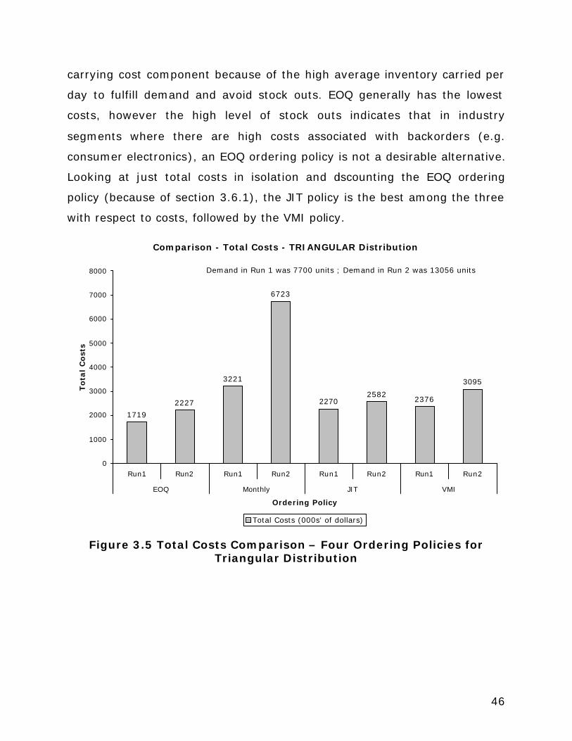
46

carrying cost component because of the high average inventory carried per

day to fulfill demand and avoid stock outs. EOQ generally has the lowest

costs, however the high level of stock outs indicates that in industry

segments where there are high costs associated with backorders (e.g.

consumer electronics), an EOQ ordering policy is not a desirable alternative.

Looking at just total costs in isolation and discounting the EOQ ordering

policy (because of section 3.6.1), the JIT policy is the best among the three

with respect to costs, followed by the VMI policy.

Comparison - Total Costs - TRIANGULAR Distribution

1719

2227

3221

6723

22702582

2376

3095

0

1000

2000

3000

4000

5000

6000

7000

8000

Run1 Run2 Run1 Run2 Run1 Run2 Run1 Run2

EOQ Monthly JIT VMI

Ordering Policy

Tota

l C

ost

s

Total Costs (000s' of dollars)

Demand in Run 1 was 7700 units ; Demand in Run 2 was 13056 units

Figure 3.5 Total Costs Comparison – Four Ordering Policies for Triangular Distribution

47

Comparison - Total Costs - POISSON Distribution

1865

2326

3669

6570

2437 2577

1907

3532

0

1000

2000

3000

4000

5000

6000

7000

Run1 Run2 Run1 Run2 Run1 Run2 Run1 Run2

EOQ Monthly JIT VMI

Ordering Policy

To

tal

Co

sts

(00

0s'

of

do

llars

)

Total Costs

Demand in Run 1 was 9100 units ; Demand in Run 2 was 12577 units

Figure 3.6 Total Costs Comparison – Four Ordering Polices for

Poisson Distribution

3.6.3 Average Daily Inventory Comparison across the three demand

distribution functions

Figures 3.7 through 3.9 illustrate the average daily inventory carried

when compared across the three demand distribution functions for the four

ordering policies. EOQ based ordering policies have the lowest average

inventory, however, this is due to the large number of days items are back

ordered (115 days of the fiscal year, on average). Monthly ordering policies

avoid backorders in the system by having large inventories at the start of

the month.

48

Comparison - Average Inventory/Day - UNIFORM DISTRIBUTION

202 172

1158

796

124164

326262

0

200

400

600

800

1000

1200

1400

Run1 Run2 Run1 Run2 Run1 Run2 Run1 Run2

EOQ Monthly JIT VMI

Ordering Policy

Avera

ge I

nven

tory

/D

ay

UNIFORM Average Inventory

Demand in Run 1 was 9261 units ; Demand in Run 2 was 14704 units

Figure 3.7 Average Daily Inventory – Uniform Distribution

Comparison - Average Inventory/Day - Triangular Distribution

171

53

731

224178

140

248

335

0

100

200

300

400

500

600

700

800

Run1 Run2 Run1 Run2 Run1 Run2 Run1 Run2

EOQ Monthly JIT VMI

Ordering Policy

Avera

ge I

nven

tory

/D

ay

Average Inventory/Day

Demand in Run 1 was 13056 units ; Demand in Run 2 was 7700 units

Figure 3.8 Average Daily Inventory – Triangular Distribution

49

Comparison - Average Inventory/Day - Poisson Distribution

60

184

393

714

125 140

360

192

0

100

200

300

400

500

600

700

800

Run1 Run2 Run1 Run2 Run1 Run2 Run1 Run2

EOQ Monthly JIT VMI

Ordering Policy

Avera

ge I

nven

tory

/D

ay

Average Inventory/Day

Demand in Run 1 was 9100 units ; Demand in Run 2 was 12577 units

Figure 3.9 Average Daily Inventory – Poisson Distribution

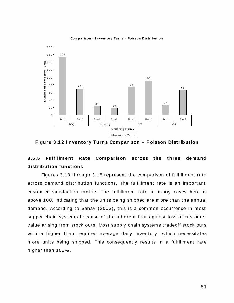
3.6.4 Inventory Turns Comparison across the three demand

distribution functions

Figures 3.10 through 3.12 represent the comparison of inventory turns

across demand distribution functions. The number of times an inventory

turns over in a year is an important performance metric in certain industry

segments, like consumer electronics. The number of inventory turns is a

performance metric that can be benchmarked against industry competitors.

50

Comparison - Inventory Turns - UNIFORM Distribution

46

86

8

19

75

90

29

57

0

10

20

30

40

50

60

70

80

90

100

Run1 Run2 Run1 Run2 Run1 Run2 Run1 Run2

EOQ Monthly JIT VMI

Ordering Policy

Nu

mb

er

of

Inven

tory

Tu

rns

Inventory Turns

Figure 3.10 Inventory Turns Comparison – Uniform Distribution

Comparison - Inventory Turns - Triangular Distribution

148

77

2318

55

74

23

53

0

20

40

60

80

100

120

140

160

Run1 Run2 Run1 Run2 Run1 Run2 Run1 Run2

EOQ Monthly JIT VMI

Ordering Policy

Nu

mb

er

of

Inven

tory

Tu

rns

Inventory Turns Figure 3.11 Inventory Turns Comparison – Triangular Distribution

51

Comparison - Inventory Turns - Poisson Distribution

154

69

2418

73

90

26

66

0

20

40

60

80

100

120

140

160

180

Run1 Run2 Run1 Run2 Run1 Run2 Run1 Run2

EOQ Monthly JIT VMI

Ordering Policy

Nu

mb

er

of

Inven

tory

Tu

rns

Inventory Turns Figure 3.12 Inventory Turns Comparison – Poisson Distribution

3.6.5 Fulfillment Rate Comparison across the three demand

distribution functions

Figures 3.13 through 3.15 represent the comparison of fulfillment rate

across demand distribution functions. The fulfillment rate is an important

customer satisfaction metric. The fulfillment rate in many cases here is

above 100, indicating that the units being shipped are more than the annual

demand. According to Sahay (2003), this is a common occurrence in most

supply chain systems because of the inherent fear against loss of customer

value arising from stock outs. Most supply chain systems tradeoff stock outs

with a higher than required average daily inventory, which necessitates

more units being shipped. This consequently results in a fulfillment rate

higher than 100%.

52

Fulfillment Rate - Uniform Distribution

96

97.97

112.3

100

103

113.55

100.42 100.78

85

90

95

100

105

110

115

Run1 Run2 Run1 Run2 Run1 Run2 Run1 Run2

EOQ Monthly JIT VMI

Ordering Policy

Fu

lfillm

en

t R

ate

Fulfillment Rate

Figure 3.13 Fulfillment Rate Comparison – Uniform Distribution

Fulfillment Rate - Triangular Distribution

96.43 99.11104.68

100.18

152.05

125

87.7

101

0

20

40

60

80

100

120

140

160

Run1 Run2 Run1 Run2 Run1 Run2 Run1 Run2

EOQ Monthly JIT VMI

Ordering Policy

Fu

lfil

lmen

t R

ate

Fulfillment Rate

Figure 3.14 Fulfillment Rate Comparison – Triangular Distribution

53

Fulfillment Rate - Poisson Distribution

96.92101

96.92 99.66

128.72

113.6

97.06 99.22

0

20

40

60

80

100

120

140

Run1 Run2 Run1 Run2 Run1 Run2 Run1 Run2

EOQ Monthly JIT VMI

Ordering Policy

Fu

lfillm

en

t R

ate

Fulfillment Rate

Figure 3.15 Fulfillment Rate Comparison – Poisson Distribution

3.6.6 Service Efficiency Level Comparison across the three demand

distribution functions

Figures 3.16 through 3.18 illustrate the service efficiency levels for the

four ordering policies. Since the monthly ordering policy involves large daily

inventories, there are almost no stock outs in a monthly ordering system.

Looking at the service efficiency levels in isolation, the monthly ordering

policy is the best. Table 3.11 provides a comparison of the average

inventory carried and the service efficiency level. D1 and D2 refer to demand

datasets 1 and 2, respectively. Figures 3.19 through 3.21 represent a

comparative idea of the average inventory carried and the corresponding

service efficiency across the demand distribution functions. Table 3.11

illustrates the fact that monthly ordering policies provide high service

efficiency levels at the cost of high daily average inventories.

54

Table 3.11 Comparative analysis – Service Efficiency and average inventory carried

EOQ MONTHLY JIT VMI

Average

Inventory SEL Average

Inventory SEL Average

Inventory SEL Average

Inventory SEL

UNIFORM DISTRIBUTION D1 202 21 1158 100 124 89 326 96 D2 172 57 796 100 164 99 262 94

TRIANGULAR DISTRIBUTION D1 171 274 731 96 178 100 248 97 D2 53 62 224 100 140 100 335 100

POISSON DISTRIBUTION D1 60 27 393 96 125 100 360 99 D2 184 64 714 100 140 99 192 86

(D1 and D2 refer to Demand datasets 1 and 2 respectively)

Service Efficiency Level - Uniform Distribution

20.27

57

100 100

89.04

99.7295.34 93.97

0

20

40

60

80

100

120

Run1 Run2 Run1 Run2 Run1 Run2 Run1 Run2

EOQ Monthly JIT VMI

Ordering Policy

SE

L

Service Efficiency Level

Figure 3.16 Service Efficiency Level Comparison – Uniform Distribution

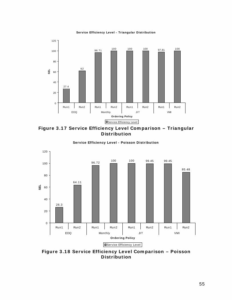
55

Service Efficiency Level - Triangular Distribution

27.4

62

96.71100 100 100 97.81 100

0

20

40

60

80

100

120

Run1 Run2 Run1 Run2 Run1 Run2 Run1 Run2

EOQ Monthly JIT VMI

Ordering Policy

SE

L

Service Efficiency Level Figure 3.17 Service Efficiency Level Comparison – Triangular

Distribution

Service Efficiency Level - Poisson Distribution

26.3

64.11

96.72100 100 99.45 99.45

85.48

0

20

40

60

80

100

120

Run1 Run2 Run1 Run2 Run1 Run2 Run1 Run2

EOQ Monthly JIT VMI

Ordering Policy

SEL

Service Efficiency Level

Figure 3.18 Service Efficiency Level Comparison – Poisson Distribution

56

Comparison - Average Inventory and Service Efficiency

202

1158

124

326

21100 89 96

172

796

164

262

57100 99 94

0

200

400

600

800

1000

1200

1400

EOQ MONTHLY JIT VMI

Ave

rage

Inve

ntor

y, S

ELAverage Inventory- D1 SEL-D1 Average Inventory - D2 SEL-D2

Figure 3.19 Comparison of Average Inventory and Service Efficiency Level – Uniform Distribution

Comparison - Average Inventory and Service Efficiency

171

731

178

248

28

96 100 97

53

224

140

335

62100 100 100

0

100

200

300

400

500

600

700

800

EOQ MONTHLY JIT VMI

Avera

ge I

nven

tory

, S

EL

Average Inventory - D1 Service Efficiency - D1 Average Inventory - D2 Service Efficiency - D2

Figure 3.20 Comparison of Average Inventory and Service Efficiency

Level – Triangular Distribution

57

Comparison - Average Inventory and Service Efficiency

60

393

125

360

27

96 100 9984

714

140

192

64100 99 86

0

100

200

300

400

500

600

700

800

EOQ MONTHLY JIT VMI

Avera

ge I

nven

tory

, S

EL

Average Inventory - D1 SEL - D1 Average Inventory - D2 SEL-D2

Figure 3.21 Comparison of Average Inventory and Service Efficiency Level – Triangular Distribution

3.7 DEVELOPMENT OF A BEST ALTERNATIVE ORDERING POLICY

Sections 3.4 and 3.5 reveal that among the four policies, the JIT and

the VMI policies are the best. For the current datasets, monthly ordering

policies are discounted because of the high inventory carrying costs and the

large amount of daily inventory carried. Sahay (2002) and Goyal (2002)

have shown that large inventories, particularly in industry segments like

consumer electronics can lead to failure of the organization. EOQ based

ordering polices are reactive in nature and exhibit a large number of stock

outs. Both JIT and VMI ordering policies have the least cost and the best

performance characteristics with respect to inventory replenishment

decisions.

58

3.7.1 Single Supplier Strategy O’Neal (1987) pointed out that the implementation of a JIT ordering

policy results in a shift to fewer suppliers, with a majority of organizations

following JIT using single-point sourcing. In the current globalization

paradigm, single-point sourcing might be cost-attractive, however, Lewis

(2000) conducted a survey of over 900 organizations, spread over a variety

of fields like service, manufacturing and retail, and concluded that moving

toward single supplier strategies does not leverage cost and performance

effectiveness opportunities. Although it is generally believed that single

supplier sourcing promotes greater commitment, in reality single supplier

sourcing leads to sub-optimization of supply chains by price discounting,

bulk volume discounts and monopolistic strategies (Sahay, 2002). Many

organizations, like Dell and HP, have realized that it is best to move to

strategic partnership relationships (like VMI entails) rather than stick to a

JIT-preferred single supplier strategy.

3.7.2 Change in Shipment Policies The increase in delivery frequencies in a JIT system typically results in

smaller quantities per shipment, often causing a shift from FTL to LTL

shipments. Additionally, it requires faster and more precise deliveries putting

more pressure on the carrier firm (Ramasesh, 1993).

Figure 3.22 illustrates that a JIT ordering policy exhibits large variation

in both supplier quantities and number of deliveries. Since the ordering

policy requires the inventory levels to be replenished at a level of 200 units

of inventory with weekly deliveries, a JIT ordering policy experiences large

variation in the number of units/shipment in the case of a change in demand

(Figure 3.20). Although no literature exists on the effect of large scale

variations in supplier deliveries on supply chain performance, Sahay (2002)

conducted a comprehensive survey which indicates that suppliers tend to opt

out of a JIT arrangement in the long run. Coupled with a single sourcing

59

strategy prevalent in most JIT supply chains, this development could spell

doom for the supply chain network.

Figure 3.22 Variation in shipment quantities in JIT Policy Table 3.12 illustrates the total quantity shipped in a JIT policy for the

three demand distribution functions. The demand dataset under

consideration is 1. The difference in the ordering quantities is reflected in the

standard deviation whereas the mean represents the average number of

units per JIT shipment.

Table 3.12 Variation in shipment quantities in JIT policy – system summary

Uniform Triangular Poisson Total Quantity Shipped 9538 11708 11713 Standard Deviation 54.38 9.18 4.37 Mean 183.43 221 225.25

Shipment Quantities - JIT Policy

50

100

150

200

250

300

0 10 20 30 40 50 60 Number of Shipments

Quantity Shipped

Uniform Distribution Triangular Distribution Poisson Distribution

60

Units/Shipment - JIT Policy

149

175 179

242252

283

0

50

100

150

200

250

300

7700 9100 9261 12577 13056 14704

Annual Demand

Un

its/

Sh

ipm

en

t

Units/Shipment

Standard Deviation 52.83

Figure 3.23 Units/Shipment in a JIT ordering policy

Figure 3.24 illustrates the difference in shipment quantities between a

JIT and a VMI policy for differing levels of annual demand. JIT policies

consistently involve not only more items shipped, but also more shipments

(Figure 3.25). With increasing globalization of supply chains, JIT ordering

policies can involve substantial costs with respect to transportation. Figure

3.25 also illustrates that, instead of proactively dealing with increasing

demand, a JIT ordering policy continues to use weekly delivery schedules

that lead to a large variance in shipment quantities. In the case of a sudden

spike or decrease in demand, tremendous pressure is placed on the delivery

carrier to maximize transportation capacity with minimal costs. JIT ordering

policies are often a refinement of EOQ based policies (Sandhwani, 1994).

61

Comparison - VMI and JIT Shipment Quantities

6753

88339300

1248013130

14820

11708 11713

9538

14286

16532 16697

7700 9100 9261 12577 13056 14704

Annual Demand

To

tal Q

uan

tity

Sh

ipp

ed

VMI JIT

Figure 3.24 Comparison of VMI and JIT shipment quantities

Number of Shipments - JIT & VMI

12 1214

2624

26

52 52 52 52 52 52

0

10

20

30

40

50

60

7700 9100 9261 12577 13056 14704

Annual Demand

Nu

mb

er

of

ship

men

ts

VMI Shipments JIT Shipments

Figure 3.25 Comparison of number of shipments – JIT & VMI

62

Figure 3.26 shows the difference between shipping in FTL and LTL

modes in JIT ordering policies. Figure 3.27 portrays the use of FTL shipping

at the cost of reduced transportation capacity utilization. Transportation

capacity utilization is the ratio of the average units/shipment to one FTL

truck capacity (assumed in this case to be 1000 units). JIT organizations

often use FTL shipping to minimize transportation costs, forgetting that use

of FTL shipments for frequent deliveries leads to a dramatic drop in

transportation capacity utilization (Yang, 2003).

Comparison of Freight Costs

1300000 1300000 1325000

260000 260000 265000

0

200000

400000

600000

800000

1000000

1200000

1400000

Normal Poisson Triangular

Distribution Function

$ D

oll

ars

LTL FTL

Figure 3.26 Difference in using FTL and LTL shipment modes for

the JIT ordering policy

63

67

18.34

73.51

22.53

57

22.09

0

10

20

30

40

50

60

70

80

% utilization

Normal Poisson TriangularDemand Distribution

Transportation capacity utilization

VMI JIT 1 FTL shipment capacity = 1000 units

Figure 3.27 Transportation capacity utilization comparison

3.7.3 Inventory Re-Routing Sandhwani (1994) used a spreadsheet solution to illustrate that the

inventory reduction in JIT policies is merely the result of pushing inventory

back into the distribution channels so that it is held by the supplier.

An examination of the average inventory between the JIT and the VMI

policy indicates that the VMI policy has higher average inventory than the

JIT policy.

64

Average Inventory Comparison

326

360338

124 125140

0

50

100

150

200

250

300

350

400

Normal Poisson Triangular

Demand Distribution Function

Un

its

of

Inven

tory

VMI JIT

Figure 3.28 Average Inventory Comparisons

Yang (2003) showed a high correlation between the inventory levels

and service efficiency (measured in terms of system stock outs). Figure 3.29

graphically illustrates the service efficiency level of the two policies. The

service efficiency levels of the two policies are more or less similar across

the three distribution functions. This indicates that the JIT policy has

inventory buffers to protect the system against stock outs. Unlike the VMI

policy which uses supplier collaboration and third party distribution centers,

JIT pushes the inventory buffers in the distribution channel to keep

inventory costs low (Sandhwani, 1994).

65

Figure 3.29 Service efficiency Comparison – JIT and VMI

S E refers to the Service Efficiency

Service Efficiency Level

95.35

99.45 97.81

89.04

100 100

82 84 86 88 90 92 94 96 98

100 102

Uniform Poisson Triangular Demand Distribution Function

S E

VMI JIT

66

CHAPTER 4. CONCLUSIONS

4.1 SUMMARY

The goal of the thesis is to develop a best alternative ordering policy

for a single manufacturer-single supplier supply chain. This thesis provides a

basic understanding with respect to the development of an ordering policy

for a single manufacturer-single supplier supply chain with known lead time

and variable demand. This was answered in two steps. First, a database

application system was constructed incorporating VMI logic. Second, using

the results from the database systems, a best alternative ordering policy for

a single manufacturer-single supplier system was developed using statistical

analysis of four ordering policies – EOQ, Monthly, JIT and VMI-under three

demand distribution functions – Uniform, Triangular and Poisson. This

analysis involved comparing the performance of the four ordering policies

under the three demand distribution functions under a variety of inventory

performance measures. All the cost data have been assumed from Goyal

(2002). The software used for the analysis was Microsoft Excel. The planning

horizon for the system was one calendar year. Once the data were set up in

spreadsheets, 2 axis graphs were used for policy comparisons. Two sets of

demand data have been used for each ordering policy.

4.2 FINDINGS FROM THE CURRENT DEMAND DATA

There is no one single answer with respect to the development of a

best alternative ordering policy for a single manufacturer-single supplier

supply chain system operating under known lead time and variable demand.

For the current dataset, using results from Suri (2002), the EOQ based

ordering policy is discounted because in each case, the coefficient of

variation is greater than 0.2. The monthly ordering policy provides high

levels of service efficiency at the cost of high inventory carrying costs.

Monthly ordering policies are useful only in situations where an organization

67

needs service efficiency of close to 100% and it is worthwhile to carry high

daily inventories to meet the service efficiency levels. Sandhwani (1994)

used a spreadsheet solution to illustrate that the inventory reduction in JIT

policies is merely the result of pushing inventory back into the distribution

channels so that it is held by the supplier. For the current datasets, section

3.7.2 illustrates that, instead of proactively dealing with increasing demand,

a JIT ordering policy continues to use weekly delivery schedules that lead to

a large variance in shipment quantities. In the case of a sudden spike or

decrease in demand, tremendous pressure is placed on the delivery carrier

to maximize transportation capacity with minimal costs. The results in

section 3.5 and 3.6 are for the two demand datasets. Although the demand

datasets have been randomly generated, the costs are assumed values from

the literature. The results would change for a different set of assumed

values.

4.3 SUPPLY CHAIN OF THE FUTURE

The key point in this research is that coordination is the key to survival in

today’s global, dynamic environment. Operations managers are faced with

demands to improve service levels while simultaneously lowering costs.

Managers are faced with managing increasingly complex supply chain

networks that include multiple suppliers, manufacturing sources,

warehouses, and transportation providers; not to mention an array of

product variations. Coordination among these disparate players is key to

success. It is no longer acceptable to create plans for only one enterprise.

Traditional distribution requirements planning (DRP) tools are not up to

today’s planning challenge because DRP creates distribution plans without

considering the costs and constraints that exist within logistics networks. It

is important to note that there is no single correct answer in supply chain

management. It is important to look at supply chain systems from a holistic

68

view. Too often, supply chain managers break a system into constituent

parts and then vertically integrate it upward without focusing on the system

interfaces. It is the management of these system interfaces, like the

interface between production and distribution that will define the success or

failure of organizations in the future. It is only a collaborative effort between

all the supply chain constituents that could create a “synchronized supply

chain.”

A supply chain of the future should address the flaws in current systems

by producing,

• a collaborative, real-time process that links customers, suppliers and

partners together, reducing the overall process cycle-time,

• a tactical plan that takes into account multiple sites, costs, constraints,

real-time inputs, and actions,

• a schedule that is “forward” looking and allows for realistic completion

dates,

• a way to accommodate customer demands while keeping sight of

business goals,

• a plan that optimizes capacity and in the process, decreases costs and

increases the bottom line,

• a system that produces actions and alerts that are meaningful, prioritized

and related to all levels of the system, thus showing planners the best

way to solve problems, and

• a plan that takes into account variable lead times and considers multiple

ways to manufacture products and can take into account possible

substitutions in real-time.

69

4.4 FURTHER DIRECTIONS FOR RESEARCH

The entire VMI system has limitations with respect to the assumptions,

particularly those related to inventory costs. These costs are assumed values

and the accuracy and precision of the results are bounded by the

assumptions behind these costs. The VMI system can be further enhanced

by the use of mechanisms to reflect dynamic pricing and the ability to vary

cost information and analyze new results. External factors like customer

satisfaction, global economic demands, adverse weather affecting loss of

shipments, etc have to be built into the system so that a truly collaborative

supply chain system can be formed. The VMI system also further needs to

be studied in the case of variable lead time. Since forecasting is the engine

that drives any sort of production, it is also important to incorporate a

forecasting module, particularly a collaborative forecasting and

replenishment model in the VMI system which acts as the driver for

production. Finally, the entire application system needs to be tested in an

actual organization to understand the practical considerations behind

implementation of a VMI strategy. This implementation also needs to include

actual performance benchmarking against the system the company is

actually using.

Finally, this thesis includes a demonstration VMI system. It also

includes performance analysis of the VMI system when compared to other

known ordering policies. The study done for this thesis will be a strong

platform for someone who is interested in working in collaborative supply

chain management. Using the conceptual framework in this thesis as a base,

a thorough VMI system can be built.

70

REFERENCES

Anderson, D., Lee, H., (1999), “Synchronized supply chains: the new frontiers”, Achieving supply chain excellence through technology, Montgomery Research. Axsater, S (2002), “A note on stock replenishment and shipment scheduling for vendor managed inventory systems”, Management Science, Vol. 47, No. 9, September 2001, pp 1306-1310. Beamon, Benita M. (2000). "Measuring Supply Chain Performance", International Journal of Operations and Production Management, Vol. 19, No. 3, pp. 275-292. (Reprinted in The Journal of Enterprise Resource Management, Vol. 7, No. 3, pp. 46-63). Cachon, G (2001), “Managing a Retailer’s shelf space, inventory and transportation”, Manufacturing & Service Operations Management, 2001 INFORMS, Volume 3, No. 3, Summer 2001, pp 211-229. Centikaya, S and C Lee (2000), “Stock replenishment and shipment scheduling for vendor managed inventory systems”, Management Science, Vol 46, No. 2, pp 217-232. Christopher, M (1999), “Logistics and supply chain management: Strategies for reducing cost and improving service”, Pittman Publishing, London. Cooke, J.A (1998), “VMI – very mixed impact”, Logistics Management and Distribution Report, Vol. 37, No. 12, pp 51-53. Cooke, J (1998), “Into the great wide open”, Logistics Management and Distribution Report, Vol. 37, No. 10, pp 84-87. Corbett (1999), “A Primer on Supply chain Management”, Information Strategy: The Executive’s Journal, winter 1999, pp 1-9. Cottrill, K (1997), “Reforging the supply chain”, Journal of Business Strategy, November-December, Vol. 18, No. 6, pp 35-39. Crainic, T. (2000), “Service network design in freight transportation”, European Journal of Operational Research 122 (2000) pp. 272-288. Dong, Y, Xu, K (2002), “A supply chain model for a vendor managed in inventory system”, Transportation Research and Logistics, Vol. 38, No. 2, April 2002, pp 75-95.

71

Fraza, V (1998), “Streamlining the channel”, Industrial Distribution, Vol. 87, No. 9, pp 73-74. Goyal, S., Nebebe, F. (2002), “Determination of economic production-shipment policy for a single-vendor-single-buyer system”, European Journal of Operational Research 121 (2002) pp. 175-178. Hall, C (1998), “What is VMI?”, Vendor Managed Inventory Web Resource, www.vendormanagedinventory.com. Harrington, L. (1996), “Consignment selling: trend or Another wild idea?”, Transportation and Distribution 37(6), pp 45-48. Holmstrom, M (1999), “Improving supply chain efficiency with postponement and vendor managed inventory”, Helsinki University of Technology. Holmstrom, J (1998), “Implementing vendor managed inventory the efficient way”, Production and Inventory Management Journal, Falls Church, Third Quarter, Vol. 39, No. 3, pp 1-5. Horvath, L (2001), “Collaboration: the key to value creation in supply chain management”, Supply Chain Management, Vol. 6, No. 5, 2001, pp 205-207. Joglekar, P. (1988), “Comments on a quantity discount pricing model to increase vendor profits”, Management Science, 34 (110), pp 1391-1398. Julia, M (2003), “Class Notes: ME 657, Modeling and Analysis of Enterprise systems”, University of Texas at Austin, Fall 2003. Kaipia, R (2002), “VMI: What are you losing if you let your customer place orders?”, Production Planning & Control, 2002, Vol. 13, No. 1, pp 17-25. Kaplan, R., Norton, S (1996), “The Balanced Scorecard: Translating Strategy into Action”, Harvard Business School Press. Kohli, R. Park, H (1994), “Coordinating buyer-seller transactions across multiple products”, Management Science 40(9), pp 45-50. Lee, H.L., Padmanabhan, V., Taylor, T.A and Whang, S (1997), “Information distortion in a supply chain: the bullwhip effect”, Management Science, Vol. 43, pp 546-558.

72

Lewis, M (2000), “Lean production and sustainable competitive advantage”, International Journal of Production and Operations Management, Vol. 20, No. 8, pp 959-978. Nolan, K (1998), “With distributors in mind, Northwestern embraces VMI”, Metal Center News, Vol. 38, No. 3, pp 32-36. O’ Neal, C.R. (1987), “The buyer-seller linkage in a just-in-time environment”, Journal of Purchasing and Materials Management, Spring 1987. Ramasesh, R (1993), “A logistics based inventory model for JIT procurement”, International Journal of Operations and Production Management, Volume 13(6), 1993, pp 1108-1221. Sahay, B (2003), “Supply chain collaboration: the key to value creation”, Work Study, Volume 52, No. 2, 2003, pp 76-83. Sandhwani, A.T., Sarhan, M.H., Camp, R.A. (1994), “The impact of just in time inventory systems on small businesses”, Journal of Accountancy, Jan 1994. Schenck, J., McInerney, J (1998), “Applying vendor managed inventory to the apparel industry”, Automatic I.D News 14(6), pp 36-38. Suri, R (2002), “Quick Response Manufacturing: A competitive strategy for the 21st century”, Advanced Manufacturing Journal, May 2002. Waller, M, Johnson, E., Davis, T (1999), “Vendor managed inventory in the retail supply chain”, Journal of Business Logistics, Vol. 20, No. 1, pp 183-203. Weng, Z.K (1995), “Channel coordination and quantity discounts”, Management Science 41(9), pp 1509-1522. Yang, C (2003), “A general framework of supply chain contract models”, Supply chain management: an international journal, Vol. 7, No. 5, 2003, pp 302-310. Zimmerman, K.A (1998), “Schnucks, Nabisco plan forecasting pilot”, Supermarket news, Vol. 48, No. 40, October, pp 71-78.

73

APPENDIX

Appendixes A through C give the inventory availability calculations for

the first thirty five days for each of the three demand distribution functions.

APPENDIX A – UNIFORM DISTRIBUTION Inventory Availability

Days Date Demand EOQ Monthly JIT VMI 1 1-Jan 42 158 1384 285 728 2 2-Jan 36 122 1348 249 692 3 3-Jan 41 81 1307 208 654 4 4-Jan 45 36 1262 163 606 5 5-Jan 44 -8 1218 119 562 6 6-Jan 41 -49 1177 79 521 7 7-Jan 39 -88 1138 39 482 8 8-Jan 37 -125 1101 285 445 9 9-Jan 38 -163 1063 247 407 10 10-Jan 38 -201 1025 209 369 11 11-Jan 42 -243 983 167 327 12 12-Jan 45 -288 938 122 282 13 13-Jan 41 357 897 81 241 14 14-Jan 44 313 853 37 197 15 15-Jan 36 277 817 285 161 16 16-Jan 45 232 772 240 116 17 17-Jan 38 194 734 202 78 18 18-Jan 44 150 690 158 604 19 19-Jan 36 114 654 122 568 20 20-Jan 39 75 645 83 529 21 21-Jan 40 35 575 43 489 22 22-Jan 37 -2 538 285 452 23 23-Jan 37 -39 504 248 415 24 24-Jan 36 -75 465 212 379 25 25-Jan 39 -114 426 173 340 26 26-Jan 43 -157 383 130 297 27 27-Jan 43 -200 340 87 254 28 28-Jan 47 -245 295 42 209 29 29-Jan 40 -285 255 285 169 30 30-Jan 43 358 212 248 129 31 31-Jan 38 320 174 212 88 32 1-Feb 40 280 130 173 48 33 2-Feb 45 235 1315 130 3 34 3-Feb 36 199 1279 87 537 35 4-Feb 40 159 1239 42 497

74

APPENDIX B – TRIANGULAR DISTRIBUTION Inventory Availability

Days Date Demand EOQ Monthly JIT VMI 1 1-Jan 38 162 162 285 667 2 2-Jan 39 123 123 246 628 3 3-Jan 34 89 89 212 594 4 4-Jan 33 56 56 179 561 5 5-Jan 39 17 17 140 522 6 6-Jan 32 -15 -15 108 490 7 7-Jan 38 -53 -53 70 452 8 8-Jan 26 -79 -79 285 426 9 9-Jan 34 -113 -113 251 392 10 10-Jan 32 -145 -145 219 360 11 11-Jan 33 -178 -178 186 327 12 12-Jan 29 -207 -207 157 298 13 13-Jan 43 397 -250 114 255 14 14-Jan 32 365 -282 82 223 15 15-Jan 43 322 -325 285 180 16 16-Jan 31 291 -356 254 149 17 17-Jan 40 251 -396 214 109 18 18-Jan 33 218 -429 181 581 19 19-Jan 40 178 -469 141 541 20 20-Jan 35 143 -504 106 506 21 21-Jan 35 108 -539 71 471 22 22-Jan 44 64 -583 285 427 23 23-Jan 44 20 -627 241 383 24 24-Jan 36 -16 -663 205 347 25 25-Jan 36 -52 -699 169 311 26 26-Jan 45 -97 -744 124 266 27 27-Jan 37 -134 -781 87 229 28 28-Jan 41 -175 -822 46 188 29 29-Jan 28 -203 -850 285 160 30 30-Jan 36 -239 -886 249 127 31 31-Jan 27 381 -913 222 97 32 1-Feb 40 341 135 182 57 33 2-Feb 29 312 106 153 28 34 3-Feb 32 280 74 121 501 35 4-Feb 37 243 37 84 464

75

APPENDIX C – POISSON DISTRIBUTION Inventory Availability

Days Date Demand EOQ Monthly JIT VMI 1 1-Jan 29 171 1221 245 651 2 2-Jan 39 767 1182 206 612 3 3-Jan 35 732 1147 171 577 4 4-Jan 35 697 1112 136 542 5 5-Jan 34 663 1078 105 508 6 6-Jan 39 624 1039 63 469 7 7-Jan 34 590 1005 29 435 8 8-Jan 37 553 968 245 398 9 9-Jan 35 518 933 210 363 10 10-Jan 30 488 903 180 333 11 11-Jan 32 456 871 148 301 12 12-Jan 36 420 835 112 265 13 13-Jan 31 389 804 81 234 14 14-Jan 39 350 765 42 195 15 15-Jan 28 322 737 245 167 16 16-Jan 30 292 707 215 137 17 17-Jan 37 255 670 178 100 18 18-Jan 34 221 636 144 546 19 19-Jan 35 186 604 109 511 20 20-Jan 40 146 561 69 471 21 21-Jan 39 107 522 30 432 22 22-Jan 45 62 477 245 387 23 23-Jan 28 34 449 217 359 24 24-Jan 40 -9 409 177 319 25 25-Jan 34 -40 375 143 285 26 26-Jan 30 -70 345 113 255 27 27-Jan 40 -110 305 73 215 28 28-Jan 19 -129 286 54 196 29 29-Jan 34 -163 252 245 162 30 30-Jan 44 -207 208 201 118 31 31-Jan 30 398 179 171 88 32 1-Feb 32 366 1196 139 56 33 2-Feb 36 330 1160 103 20 34 3-Feb 39 291 1121 64 461 35 4-Feb 41 250 1080 23 420