UIS - Getting Started in Excel · 2013-04-22 · Overview of Excel Microsoft Excel 2010 is a powerful tool you can use to create and format spreadsheets, create graphs to visually

[Not for Circulation]

Information Technology Services, UIS 1

Getting Started in Excel

This document provides information regarding creating basic spreadsheets in Microsoft Excel

2010 – entering and formatting text and numbers as well as sorting and filtering data.

Overview of Excel

Microsoft Excel 2010 is a powerful tool you can use to create and format spreadsheets, create

graphs to visually display data, write formulas to calculate mathematical equations, and

analyze and share information to make more informed decisions.

The Font Group on the Home Tab

The Font group on the Home tab contains basic text and cell formatting tools.

The cell border tool offers many options for adding borders.

The cell border, background color, and text color buttons ‘remember’ the

most recent selection made. For example, if the last cell border you

selected was a Thick Box Border, you can just click the cell border button to

assign another cell with that border (without having to reselect it from the

dropdown list).

Change font type.

Change font size; increase or

decrease font size.

Bold, underline, or

italicize text.

Add a cell border.

Change the color of the text.

Add a background color to

the cell.



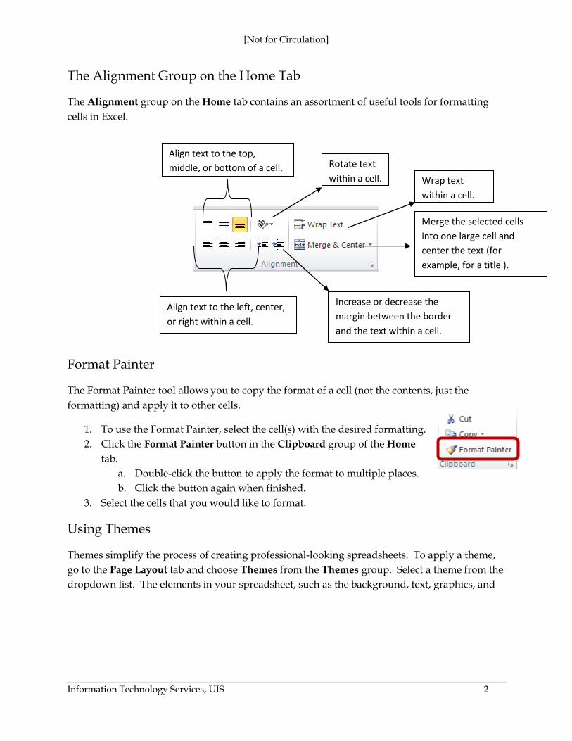
The Alignment Group on the Home Tab

The Alignment group on the Home tab contains an assortment of useful tools for formatting

cells in Excel.

Format Painter

The Format Painter tool allows you to copy the format of a cell (not the contents, just the

formatting) and apply it to other cells.

1. To use the Format Painter, select the cell(s) with the desired formatting.

2. Click the Format Painter button in the Clipboard group of the Home

tab.

a. Double-click the button to apply the format to multiple places.

b. Click the button again when finished.

3. Select the cells that you would like to format.

Using Themes

Themes simplify the process of creating professional-looking spreadsheets. To apply a theme,

go to the Page Layout tab and choose Themes from the Themes group. Select a theme from the

dropdown list. The elements in your spreadsheet, such as the background, text, graphics, and

Align text to the left, center,

or right within a cell.

Align text to the top,

middle, or bottom of a cell. Rotate text

within a cell. Wrap text

within a cell.

Increase or decrease the

margin between the border

and the text within a cell.

Merge the selected cells

into one large cell and

center the text (for

example, for a title ).



charts, will be formatted to follow that theme.

Additional Formatting Options

The Format button in the Cells group on the Home tab includes options to adjust the row

height, column width, hide and unhide rows and columns, organize sheets, add protection, and

provides a full array of additional cell formatting tools.

Adjust the row height or

column width.

Hide or unhide rows,

columns, or the sheet. Rename, move, copy, or

color the sheets (the

tabs at the bottom of

the window). Password-protect the sheet.

(Please note that if you lose the

password, you cannot gain access

to the protected elements on the

worksheet.)

Displays additional

formatting options.



The Format Cells Dialog Box

Apply a number

format.

Adjust the

alignment of the

cell contents.

Adjust the font. Apply a border.

Select a

background -

a single color,

a gradient of

colors, or a

pattern.

Choose to lock cells or hide

formulas.



Applying Cell Styles

A cell style is a defined set of formatting characteristics, such as fonts and font sizes, number

formats, cell borders, and cell shading. Excel 2007 has several built-in cell styles that you can

apply or modify. You can also modify or duplicate a cell style to create your own custom cell

style.

Cell styles are based on the document theme that is applied to the entire workbook. When you

switch to another document theme, the cell styles are updated to match the new document

theme.

1. To apply a cell style, select the cells that you want to format.

2. Go to the Home tab, in the Cells group, and select Cell Styles.

3. Click the cell style that you want to apply.

4. To create a custom style, select New Cell Style.

a. Give the style a name.



b. Click Format.

c. On the various tabs in the Format Cells dialog box, select the formatting that you

want, and then click OK.

d. In the Style dialog box, under Style Includes (By Example), clear the check

boxes for any formatting that you don't want to include in the cell style.

5. To remove a cell style from selected cells without deleting the cell style, select the cells

that are formatted with that cell style.

a. On the Home tab, in the Styles group, click Cell Styles.

b. Do one of the following:

i. To remove the cell style from the selected cells without deleting the cell

style, under Good, Bad, and Neutral, click Normal.

ii. To delete the cell style and remove it from all cells that are formatted with

it, right-click the cell style, and then click Delete.

Working with Multiple Worksheets

By default, Excel provides three worksheets in a workbook, but additional worksheets can be

inserted (the number of worksheets that can be added is limited only by your computer’s

available memory and system resources) or deleted as needed. Each worksheet has 1,048,576

rows and 16,384 columns.

The name (or title) of a worksheet appears on its sheet tab at the bottom of the screen. By

default, the name is Sheet1, Sheet2, and so on, but you can give any worksheet a more

appropriate name as well as adjust the color.



1. To add a new worksheet, click on the Insert Worksheet button at the bottom of the

screen.

2. To rename a worksheet, either double-click its name or right-click and choose Rename.

3. Navigate through the sheets by clicking on their name. You can also use the navigation

buttons to quickly flip to the first, previous, next, or last worksheet.

a. You can also right-click on the navigation buttons to see a list of worksheets by

name. To navigate to a particular worksheet, simply click on its name.

4. To change the color of a worksheet, right-click and choose Tab Color.

5. To rearrange the worksheets, simply click and drag them to the desired location.



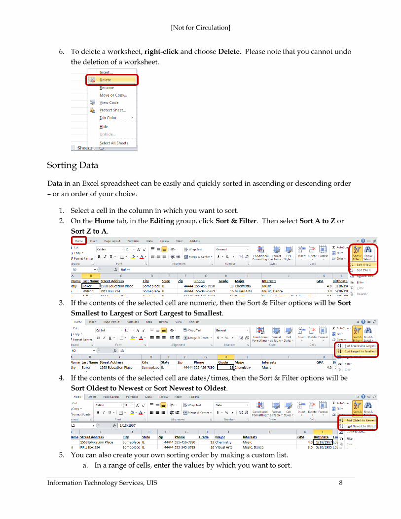
6. To delete a worksheet, right-click and choose Delete. Please note that you cannot undo

the deletion of a worksheet.

Sorting Data

Data in an Excel spreadsheet can be easily and quickly sorted in ascending or descending order

– or an order of your choice.

1. Select a cell in the column in which you want to sort.

2. On the Home tab, in the Editing group, click Sort & Filter. Then select Sort A to Z or

Sort Z to A.

3. If the contents of the selected cell are numeric, then the Sort & Filter options will be Sort

Smallest to Largest or Sort Largest to Smallest.

4. If the contents of the selected cell are dates/times, then the Sort & Filter options will be

Sort Oldest to Newest or Sort Newest to Oldest.

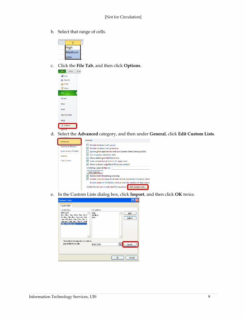
5. You can also create your own sorting order by making a custom list.

a. In a range of cells, enter the values by which you want to sort.



b. Select that range of cells.

c. Click the File Tab, and then click Options.

d. Select the Advanced category, and then under General, click Edit Custom Lists.

e. In the Custom Lists dialog box, click Import, and then click OK twice.



f. On the Home tab, in the Editing group, click Sort & Filter. Then select Custom

Sort.

g. Under Column, in the Sort by or Then by box, select the column by which you

want to apply your custom list.

h. Under Order, select Custom List.

i. In the Custom Lists dialog box, select the desired list and click OK.

Filtering Data

The ability to filter data is an invaluable resource. Filtered data displays only the rows that

meet criteria that you specify and hides rows that you do not want displayed. After you filter



data, you can copy, find, edit, format, chart, and print the subset of filtered data without

rearranging or moving it.

1. Select a cell in the range in which you want to add a filter.

2. On the Home tab, in the Editing group, click Sort & Filter. Then select Filter.

3. This adds dropdown arrows next to each title in the header row.

4. Click the dropdown arrow next to the column in which you want to apply the filter.

Using the checkboxes, select the value(s) for your criteria. Click OK.

5. Your spreadsheet will now display only records that meet the criteria. The status bar

will display a message indicating how many records were filtered. The column in which



you applied the filter is indicated by a filter icon.

6. To remove the filter, click the dropdown arrow next to the column title and click Clear

Filter From.

7. Filters can be applied to multiple columns. Filters are additive, which means that each

additional filter is based on the current filter and further reduces the subset of data. To

clear all filters, click the Sort & Filter button in the Home tab, and select Clear.

Additional Filtering Options

There are additional filtering options available, based on the content of the column (text,

numeric, or date).



1. For text cells, click the dropdown arrow next to the column title and choose Text Filters.

a. Select the appropriate filter category and fill in the blanks with your criteria.

2. For numeric cells, click the dropdown arrow next to the column title and choose

Number Filters.




3. For date cells, click the dropdown arrow next to the column title and choose Date

Filters.


4. You can also apply custom filters, which allow you to enter wildcards (like * or ?).

a. A question mark (?) wildcard allows you to find any single character. For

example, ‘r?t’ would find ‘rat’, ‘rot’, and ‘rut’.

b. An asterisk wildcard allows you to find any number of characters. For example,

‘*east’ would find ‘northeast’ and ‘southeast’.

Documents

UIS - Getting Started in Excel · 2013-04-22 · Overview of Excel Microsoft Excel 2010 is a powerful tool you can use to create and format spreadsheets, create graphs to visually