UFC 3-230-01 AC 150/5320-5C 8/1/2006 9/29/2006

CHAPTER 3

PAVEMENT SURFACE DRAINAGE

3-1 OVERVIEW. Effective drainage of pavements is essential to the maintenance of the service level and to traffic safety. Water on the pavement can interrupt traffic, reduce skid resistance, increase potential for hydroplaning, limit visibility due to splash and spray, and cause difficulty in steering a vehicle when the wheels encounter puddles.

Pavement drainage requires consideration of surface drainage, gutter flow, and inlet capacity. The design of these elements is dependent on storm frequency and the allowable spread of storm water on the pavement surface. This chapter presents design guidance for the design of these elements. Most of the information presented here is taken directly from the FHWA’s HEC-22 and AASHTO's Model Drainage Manual. The charts referenced throughout this chapter can be found in the HEC-22.

3-2 DESIGN FREQUENCY AND SPREAD. Two of the more significant variables considered in the design of pavement drainage are the frequency of the design runoff event and the allowable spread of water on the pavement. A related consideration is the use of an event of lesser frequency to check the drainage design.

Spread and design frequency are not independent. The implications of the use of a criterion for spread of one-half of a traffic lane are considerably different for one design frequency than for a lesser frequency. It also has different implications for a low-traffic, low-speed roadway than for a higher classification roadway or airport runways. These subjects are central to the issue of pavement drainage and important to highway and runway safety.

3-2.1 Selection of Design Frequency and Design Spread

3-2.1.1 The objective of storm drainage design is to provide for safe passage of vehicles during the design storm event. The design of a drainage system for a curbed pavement section is to collect runoff in the gutter and convey it to pavement inlets in a manner that provides reasonable safety for traffic and pedestrians at a reasonable cost. As spread increases, the risks of traffic accidents and delays, and the nuisance and possible hazard to pedestrian traffic increase.

3-2.1.2 The allowable spread for airfields, runways, taxiways, and aprons was defined in Chapter 2, section 2-2.4, Design Storm Frequency.

3-2.1.3 Spread on traffic lanes can be tolerated to greater widths where traffic volumes and speeds are low. Spreads of one-half of a traffic lane are usually considered a minimum type design for DOD roads.

3-2.1.4 The selection of design criteria for intermediate types of facilities may be the most difficult. For example, some arterials with relatively high traffic volumes and

40

UFC 3-230-01 AC 150/5320-5C 8/1/2006 9/29/2006

speeds may not have shoulders that will convey the design runoff without encroaching on the traffic lanes. In these instances, an assessment of the relative risks and costs of various design spreads may be helpful in selecting appropriate design criteria.

3-2.1.5 The recommended design frequency for depressed sections and underpasses where ponded water can be removed only through the storm drainage system is a 50-yr frequency event. The use of a lesser frequency event, such as a 100-yr storm, to assess hazards at critical locations where water can pond to appreciable depths is commonly referred to as a check storm or check event.

3-2.2 Selection of Check Storm and Spread

3-2.2.1 A check storm should be used any time runoff could cause unacceptable flooding during less frequent events. Also, inlets should always be evaluated for a check storm when a series of inlets terminates at a sag vertical curve where ponding to hazardous depths could occur.

3-2.2.2 The frequency selected for the check storm should be based on the same considerations used to select the design storm, i.e., the consequences of spread exceeding that chosen for design and the potential for ponding. Where no significant ponding can occur, check storms are usually unnecessary.

3-2.2.3 Criteria for spread during the check event are: (1) one lane open to traffic during the check storm event, and (2) one lane free of water during the check storm event. These criteria differ substantively, but each sets a standard by which the design can be evaluated.

3-3 SURFACE DRAINAGE. When rain falls on a sloped pavement surface, it forms a thin film of water that increases in thickness as it flows to the edge of the pavement. Factors that influence the depth of water on the pavement include the length of flow path, surface texture, surface slope, and rainfall intensity. As the depth of water on the pavement increases, the potential for vehicular hydroplaning increases. For the purposes of highway drainage, this section provides information on hydroplaning and design guidance for these drainage elements:

Longitudinal pavement slope

Cross or transverse pavement slope

Curb and gutter design

Roadside and median ditches

Note that the guidance for transverse and longitudinal slopes for military airfields is in UFC 3-260-01 and for FAA facilities, AC 150/5300-13.

3-3.1 Longitudinal Slope. Experience has shown that the recommended minimum values of roadway longitudinal slope given in the AASHTO Green Book, A Policy on

41

UFC 3-230-01 AC 150/5320-5C 8/1/2006 9/29/2006

Geometric Design of Highways and Streets, will provide safe, acceptable pavement drainage. In addition, follow these general guidelines:

A minimum longitudinal gradient is more important for a curbed pavement than for an uncurbed pavement since the water is constrained by the curb. However, flat gradients on uncurbed pavements can lead to a spread problem if vegetation is allowed to build up along the pavement edge.

Desirable gutter grades should not be less than 0.5 percent for curbed pavements, with an absolute minimum of 0.3 percent. Minimum grades can be maintained in very flat terrain by use of a rolling profile, or by warping the cross slope to achieve rolling gutter profiles.

To provide adequate drainage in sag vertical curves, a minimum slope of 0.3 percent should occur within 50 ft of the low point of the curve. This is accomplished where the length of the curve in feet divided by the algebraic difference in grades in percent (K) is equal to or less than 167. This is represented as:

12 GG LK −

= (3-1)

where:

K = vertical curve constant, ft/percent

L = horizontal length of curve, ft

Gi = grade of roadway, percent

3-3.2 Cross (Transverse) Slope. An acceptable range of roadway cross slopes is specified in UFC 3-250-01FA. These cross slopes are a compromise between the need for reasonably steep cross slopes for drainage and relatively flat cross slopes for driver comfort and safety. These cross slopes represent standard practice.

3-3.2.1 Cross slopes of 2 percent have little effect on driver effort in steering or on friction demand for vehicle stability. Use of a cross slope steeper than 2 percent on pavements with a central crown line is not desirable. In areas of intense rainfall, a somewhat steeper cross slope (2.5 percent) may be used to facilitate drainage.

3-3.2.2 Additional guidelines related to cross slope are:

Although not widely encouraged, inside lanes can be sloped toward the median if conditions warrant.

Median areas should not be drained across travel lanes.

42

UFC 3-230-01 AC 150/5320-5C 8/1/2006 9/29/2006

The number and length of flat pavement sections in cross slope transition areas should be minimized. Consideration should be given to increasing cross slopes in sag vertical curves, crest vertical curves, and in sections of flat longitudinal grades.

Shoulders should be sloped to drain away from the pavement, except with raised, narrow medians and superelevations.

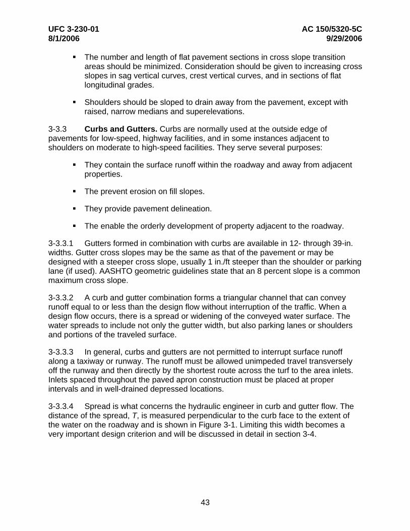
3-3.3 Curbs and Gutters. Curbs are normally used at the outside edge of pavements for low-speed, highway facilities, and in some instances adjacent to shoulders on moderate to high-speed facilities. They serve several purposes:

They contain the surface runoff within the roadway and away from adjacent properties.

The prevent erosion on fill slopes.

They provide pavement delineation.

The enable the orderly development of property adjacent to the roadway.

3-3.3.1 Gutters formed in combination with curbs are available in 12- through 39-in. widths. Gutter cross slopes may be the same as that of the pavement or may be designed with a steeper cross slope, usually 1 in./ft steeper than the shoulder or parking lane (if used). AASHTO geometric guidelines state that an 8 percent slope is a common maximum cross slope.

3-3.3.2 A curb and gutter combination forms a triangular channel that can convey runoff equal to or less than the design flow without interruption of the traffic. When a design flow occurs, there is a spread or widening of the conveyed water surface. The water spreads to include not only the gutter width, but also parking lanes or shoulders and portions of the traveled surface.

3-3.3.3 In general, curbs and gutters are not permitted to interrupt surface runoff along a taxiway or runway. The runoff must be allowed unimpeded travel transversely off the runway and then directly by the shortest route across the turf to the area inlets. Inlets spaced throughout the paved apron construction must be placed at proper intervals and in well-drained depressed locations.

3-3.3.4 Spread is what concerns the hydraulic engineer in curb and gutter flow. The distance of the spread, T, is measured perpendicular to the curb face to the extent of the water on the roadway and is shown in Figure 3-1. Limiting this width becomes a very important design criterion and will be discussed in detail in section 3-4.

43

UFC 3-230-01 AC 150/5320-5C 8/1/2006 9/29/2006

Figure 3-1. Typical Gutter Sections

3-3.3.5 Where practical, runoff from cut slopes and other areas draining toward the roadway should be intercepted before it reaches the highway. By doing so, the deposition of sediment and other debris on the roadway as well as the amount of water that must be carried in the gutter section will be minimized. Where curbs are not needed for traffic control, shallow ditch sections at the edge of the roadway pavement or shoulder offer advantages over curbed sections by providing less of a hazard to traffic than a near-vertical curb and by providing hydraulic capacity that is not dependent on spread on the pavement. These ditch sections are particularly appropriate where curbs have historically been used to prevent water from eroding fill slopes.

3-3.4 Roadside and Median Channels

3-3.4.1 Roadside channels are commonly used with uncurbed roadway sections to convey runoff from the highway pavement and from areas that drain toward the highway. Due to right-of-way limitations, roadside channels cannot be used on most urban arterials.

3-3.4.2 They can be used in cut sections, depressed sections, and other locations where sufficient right-of-way is available and driveways or intersections are infrequent.

3-3.4.3 To prevent drainage from the median areas from running across the travel lanes, slope median areas and inside shoulders to a center swale. This design is particularly important for high speed facilities and for facilities with more than two lanes of traffic in each direction.

44

UFC 3-230-01 AC 150/5320-5C 8/1/2006 9/29/2006

3-4 FLOW IN GUTTERS. A pavement gutter is defined as a section of pavement adjacent to the roadway that conveys water during a storm runoff event. It may include a portion or all of a travel lane. As illustrated in Figure 3-1, gutter sections can be categorized as conventional or shallow swale type. Conventional curb and gutter sections usually have a triangular shape, with the curb forming the near-vertical leg of the triangle. Conventional gutters may have a straight cross slope (Figure 3-1, a.1), a composite cross slope where the gutter slope varies from the pavement cross slope (Figure 3-1, a.2), or a parabolic section (Figure 3-1, a.3). Shallow swale gutters typically have V-shaped or circular sections as illustrated in Figure 3-1, b.1, b.2, and b.3, respectively, and are often used in paved median areas on roadways with inverted crowns.

3-4.1 Capacity Relationship

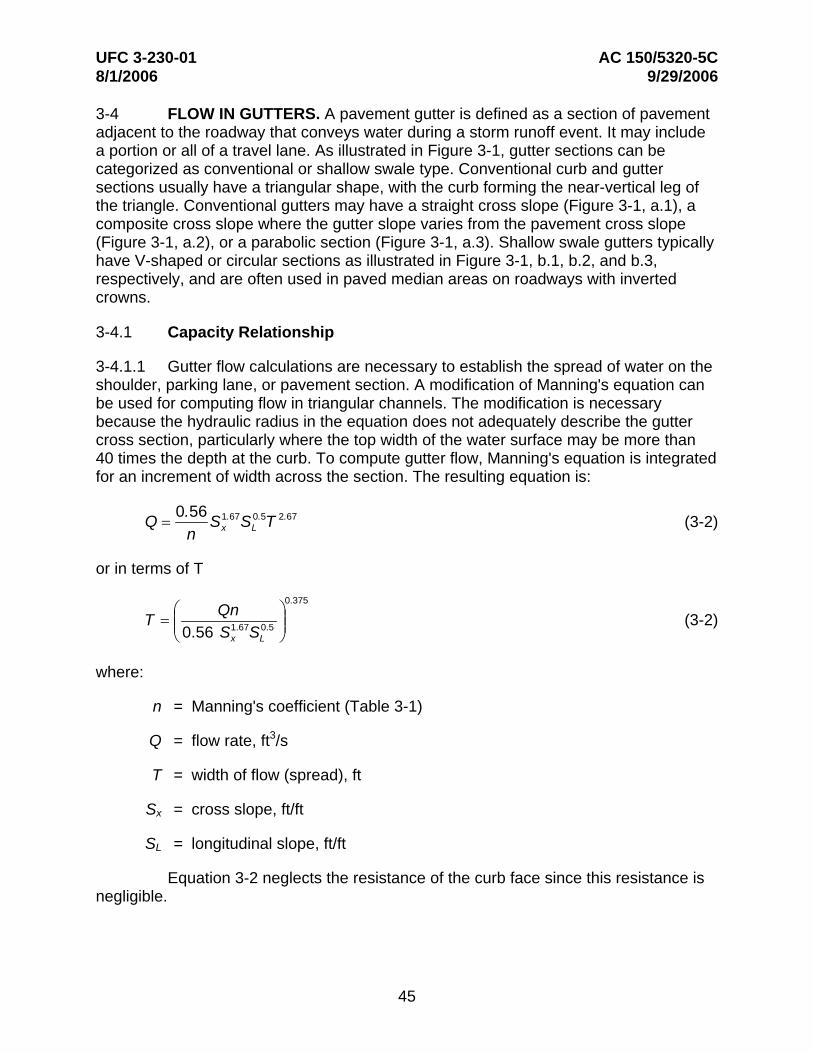
3-4.1.1 Gutter flow calculations are necessary to establish the spread of water on the shoulder, parking lane, or pavement section. A modification of Manning's equation can be used for computing flow in triangular channels. The modification is necessary because the hydraulic radius in the equation does not adequately describe the gutter cross section, particularly where the top width of the water surface may be more than 40 times the depth at the curb. To compute gutter flow, Manning's equation is integrated for an increment of width across the section. The resulting equation is:

Q = 0.56 Sx

1.67SL 0.5T 2.67 (3-2)

n

or in terms of T

0.375

T =⎛ Qn ⎞

(3-2)⎜⎜ 0.56 S1.67S0.5 ⎟⎟ ⎝ x L ⎠

where:

n = Manning's coefficient (Table 3-1)

Q = flow rate, ft3/s

T = width of flow (spread), ft

Sx = cross slope, ft/ft

SL = longitudinal slope, ft/ft

Equation 3-2 neglects the resistance of the curb face since this resistance is negligible.

45

UFC 3-230-01 AC 150/5320-5C 8/1/2006 9/29/2006

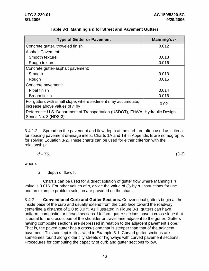
Table 3-1. Manning's n for Street and Pavement Gutters

Type of Gutter or Pavement Manning's n Concrete gutter, troweled finish 0.012 Asphalt Pavement: Smooth texture Rough texture

0.013 0.016

Concrete gutter-asphalt pavement: Smooth Rough

0.013 0.015

Concrete pavement: Float finish Broom finish

0.014 0.016

For gutters with small slope, where sediment may accumulate, increase above values of n by 0.02

Reference: U.S. Department of Transportation (USDOT), FHWA, Hydraulic Design Series No. 3 (HDS-3)

3-4.1.2 Spread on the pavement and flow depth at the curb are often used as criteria for spacing pavement drainage inlets. Charts 1A and 1B in Appendix B are nomographs for solving Equation 3-2. These charts can be used for either criterion with the relationship:

d = TSx (3-3)

where:

d = depth of flow, ft

Chart 1 can be used for a direct solution of gutter flow where Manning's n value is 0.016. For other values of n, divide the value of Qn by n. Instructions for use and an example problem solution are provided on the chart.

3-4.2 Conventional Curb and Gutter Sections. Conventional gutters begin at the inside base of the curb and usually extend from the curb face toward the roadway centerline a distance of 1.0 to 3.0 ft. As illustrated in Figure 3-1, gutters can have uniform, composite, or curved sections. Uniform gutter sections have a cross-slope that is equal to the cross-slope of the shoulder or travel lane adjacent to the gutter. Gutters having composite sections are depressed in relation to the adjacent pavement slope. That is, the paved gutter has a cross-slope that is steeper than that of the adjacent pavement. This concept is illustrated in Example 3-1. Curved gutter sections are sometimes found along older city streets or highways with curved pavement sections. Procedures for computing the capacity of curb and gutter sections follow.

46

UFC 3-230-01 AC 150/5320-5C 8/1/2006 9/29/2006

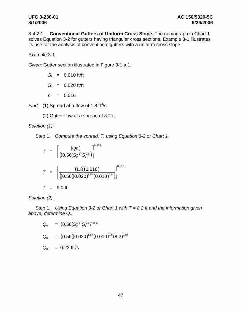
3-4.2.1 Conventional Gutters of Uniform Cross Slope. The nomograph in Chart 1 solves Equation 3-2 for gutters having triangular cross sections. Example 3-1 illustrates its use for the analysis of conventional gutters with a uniform cross slope.

Example 3-1

Given: Gutter section illustrated in Figure 3-1 a.1.

SL = 0.010 ft/ft

Sx = 0.020 ft/ft

n = 0.016

Find: (1) Spread at a flow of 1.8 ft3/s

(2) Gutter flow at a spread of 8.2 ft

Solution (1):

Step 1. Compute the spread, T, using Equation 3-2 or Chart 1.

⎡ (Qn) ⎤0.375

T = ⎢((0.56)S1.67S 0.5 )⎥⎣ x L ⎦

⎡ (1.8)( 0.016) ⎤0.375

T = ⎢{(0.56)( 0.020)1.67 (0.010)0.5 }⎥⎣ ⎦

T = 9.0 ft

Solution (2):

Step 1. Using Equation 3-2 or Chart 1 with T = 8.2 ft and the information given above, determine Qn.

1.67 0.5 2.67Qn = (0.56)Sx SL T

Qn = (0.56)( 0.020)1.67 (0.010)0.5 (8.2)2.67

Qn = 0.22 ft3/s

47

UFC 3-230-01 AC 150/5320-5C 8/1/2006 9/29/2006

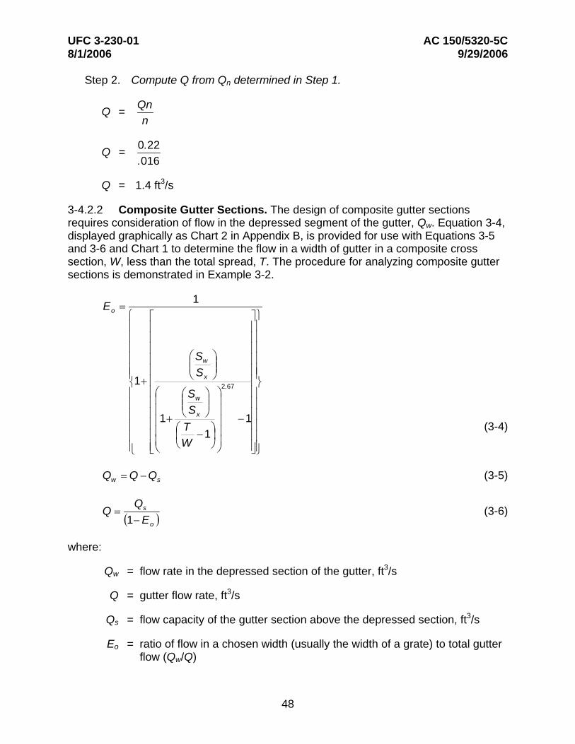
Step 2. Compute Q from Qn determined in Step 1.

Q = Qnn

0.22Q = .016

Q = 1.4 ft3/s

3-4.2.2 Composite Gutter Sections. The design of composite gutter sections requires consideration of flow in the depressed segment of the gutter, Qw. Equation 3-4, displayed graphically as Chart 2 in Appendix B, is provided for use with Equations 3-5 and 3-6 and Chart 1 to determine the flow in a width of gutter in a composite cross section, W, less than the total spread, T. The procedure for analyzing composite gutter sections is demonstrated in Example 3-2.

1Eo =⎫⎤⎡⎧

1

⎪ ⎪ ⎪ ⎪ ⎪⎪⎨

⎪ ⎪ ⎪ ⎪ ⎪⎪⎬

⎢ ⎢ ⎢ ⎢ ⎢ ⎢ ⎢ ⎢ ⎢ ⎢ ⎢ ⎢⎣

⎞⎟ ⎟ ⎟ ⎟⎟⎠

2.67

−

⎥ ⎥ ⎥ ⎥ ⎥ ⎥ ⎥ ⎥ ⎥ ⎥ ⎥ ⎥⎦

1

⎛⎜⎜⎝

⎞⎟ ⎠

⎞⎟⎠

⎟

1

Sw

Sx+⎛⎜ ⎜ ⎜ ⎜⎜

⎞⎟⎜⎠

⎛⎜ ⎝

Sw

S ⎟⎪ ⎪ ⎪ ⎪ ⎪⎪⎩

⎪ ⎪ ⎪ ⎪ ⎪⎪⎭

x1⎛⎜⎝

+(3-4)T

−W⎝

− (3-5)Qw Q Qs =

Q (3-6)Q s=(1

where:

Qw = flow rate in the depressed section of the gutter, ft3/s

Q = gutter flow rate, ft3/s

Qs = flow capacity of the gutter section above the depressed section, ft3/s

Eo = ratio of flow in a chosen width (usually the width of a grate) to total gutter flow (Qw/Q)

)−Eo

48

UFC 3-230-01 AC 150/5320-5C 8/1/2006 9/29/2006

Sw = Sx + a/W (Figure 3-1 a.2)

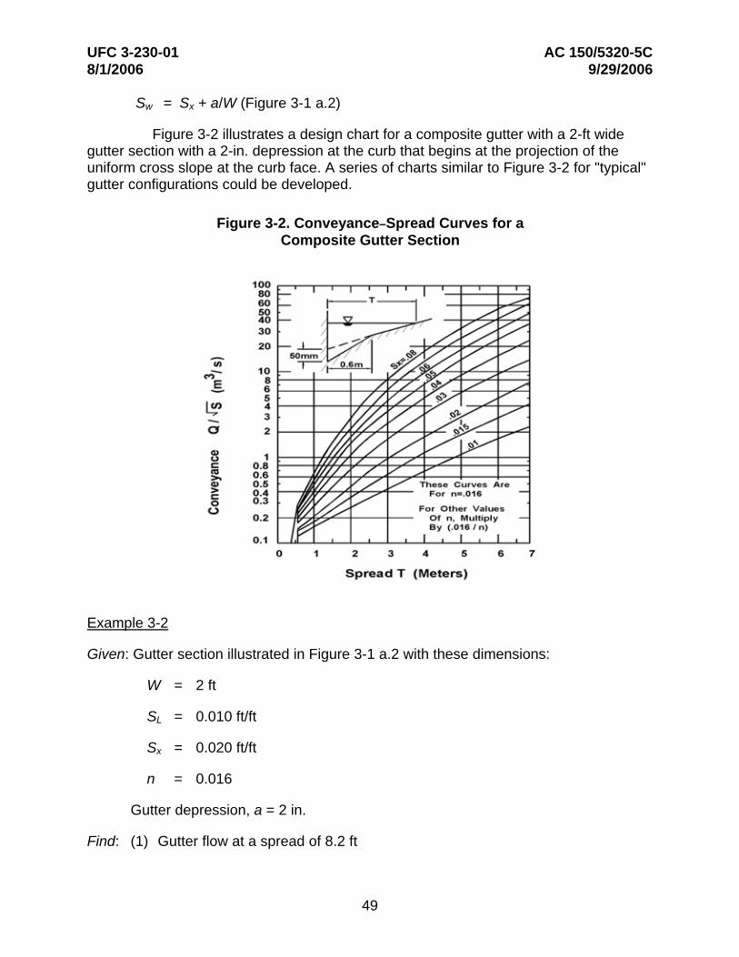
Figure 3-2 illustrates a design chart for a composite gutter with a 2-ft wide gutter section with a 2-in. depression at the curb that begins at the projection of the uniform cross slope at the curb face. A series of charts similar to Figure 3-2 for "typical" gutter configurations could be developed.

Figure 3-2. Conveyance–Spread Curves for a Composite Gutter Section

Example 3-2

Given: Gutter section illustrated in Figure 3-1 a.2 with these dimensions:

W = 2 ft

SL = 0.010 ft/ft

Sx = 0.020 ft/ft

n = 0.016

Gutter depression, a = 2 in.

Find: (1) Gutter flow at a spread of 8.2 ft

49

UFC 3-230-01 AC 150/5320-5C 8/1/2006 9/29/2006

(2) Spread at a flow of 4.2 ft3/s

Solution (1):

Step 1. Compute the cross slope of the depressed gutter, Sw, and the width of spread from the junction of the gutter and the road to the limit of the spread, Ts.

Sw = (a/W) + Sx

Sw = [( ) ( )2 / 12 ]+ (0.020)( )2

= 0.103 ft/ft

Ts = T - W = 8.2 - 2.0

Ts = 6.2 ft

Step 2. From Equation 3-2 or Chart 1 (using Ts.):

1.67 0.5 2.67Qsn = (0.56)Sx SL Ts

1.67 0.5 2.67Qsn = (0.56)( 0.02) ( 0.01) (6.2)

Qsn = 0.011 ft3/s, and

(Q n) 0.011Qs = s =n 0.016

Qs = 0.69 ft3/s

Step 3. Determine the gutter flow, Q, using Equation 3-4 or Chart 2.

T 8.2= = 4.10 W 2.0

Sw 0.103= = 5.15 S 0.020x

50

UFC 3-230-01 8/1/2006

AC 150/5320-5C 9/29/2006

1 ⎧ ⎡ ⎫⎤

⎪⎪⎪⎪ ⎪⎪⎬⎪⎪⎪ ⎪⎪⎪⎭

⎥⎥⎥⎥⎥⎥⎥⎥⎥⎥⎥⎦

2.67⎞⎞

⎟ ⎠

Sw

x

(1

Q = 2.3 ft3/s

Solution (2):

Since the spread cannot be determined by a direct solution, an iterative approach must be used.

Step 1. Try Qs = 1.4 ft3/s.

Step 2. Compute Qw.

S

⎜ ⎟1

1

⎫⎤

5.151 5.15

)

⎞⎟⎠

4.10 1

((

(

⎡⎧ ⎪⎪⎨

⎪⎪⎬⎪ ⎪⎭

⎥ ⎥ ⎥ ⎥ ⎥⎦

1−

−

2.67

⎟ ⎟ ⎟ ⎟⎟⎠

⎞⎟⎟⎠

))

0.24==T 8.2

⎞⎟⎟⎠

−

Sw

−

xS

⎛⎜⎜⎝

1

⎛⎜ ⎝

⎛

WT⎛

⎜⎝

+1

⎜ ⎜ ⎜ ⎜⎜⎝

0.70=

s

+

0.70)

1

)

⎛⎜⎜⎝

⎢⎢⎢⎢⎢⎢⎢⎢⎢⎢⎢

0.69

⎣

⎢ ⎢ ⎢ ⎢ ⎢⎣

Eo

+

+

(

QEo = w

Q

Q 1−

1

⎪⎪⎪⎪ ⎪⎪⎨⎪⎪⎪⎪⎪⎪⎩

−

⎪ ⎪⎩

Eo = 0.70

W 2.0or from Chart 2, for

Eo =

Eo =

Q =

Q =

51

UFC 3-230-01 AC 150/5320-5C 8/1/2006 9/29/2006

Qw = Q - Qs = 4.2 - 1.4

Qw = 2.8 ft3/s

Step 3. Using Equation 3-4 or from Chart 2, determine the W/T ratio.

Q 2.8Eo = w = = 0.67 Q 4.2

S 0.103w = = 5.15 S 0.020x

W = 0.23 from Chart 2 T

Step 4. Compute the spread based on the assumed Qs.

W 2.0T = = ⎛W ⎞ .23⎜ ⎟ ⎝ T ⎠

T = 8.7 ft

Step 5. Compute the Ts based on the assumed Qs.

Ts = T - W = 8.7 - 2.0 = 6.7 ft

Step 6. Use Equation 3-2 or Chart 1 to determine the Qs for the computed Ts.

Qsn = (0.56)Sx 1.67SL

0.5Ts 2.67

Qsn = (0.56)( 0.02)1.67 (0.01)0.5 (6.7)2.67

Qsn = 0.0131 ft3/s

Qsn 0.0131Qs = = n 0.016

Qs = 0.82 ft3/s

Step 7. Compare the computed Qs with the assumed Qs.

Qs assumed = 1.4 > 0.82 = Qs computed. Not close, try again.

Step 8. Try a new assumed Qs and repeat Steps 2 through 7.

52

UFC 3-230-01 AC 150/5320-5C 8/1/2006 9/29/2006

Assume Qs = 1.9 ft3/s

Qw = 4.2 - 1.9 = 2.3 ft3/s

Qw 2.3Eo = = = 0.55 Q 4.2

Sw = 5.15 Sx

W = 0.18 T

2.0T = = 11.1 ft 0.18

Ts = 11.1 - 2.0 = 9.1 ft

Qsn = 0.30 ft3/s

Qs = 0.30 = 1.85 ft3/s0.016

Qs assumed = 1.9 ft3/s close to 1.85 ft3/s = Qs computed

3-4.3 Shallow Swale Sections

3-4.3.1 Runoff Control. Where curbs are not needed for traffic control, a small swale section of circular or V shape may be used to convey runoff from the pavement. As an example, the control of pavement runoff on fills may be needed to protect the embankment from erosion. Small swale sections may have sufficient capacity to convey the flow to a location suitable for interception.

3-4.3.2 V-sections. Chart 1 can be used to compute the flow in a shallow V-shaped section. When using Chart 1 for V-shaped channels, the cross slope, Sx, is determined by Equation 3-7:

S = (SSx1

+

SSx2

2 ) (3-7)x

x1 x

Example 3-3 demonstrates the use of Chart 1 to analyze a V-shaped shoulder gutter. Analysis of a V-shaped gutter resulting from a roadway with an inverted crown section is illustrated in Example 3-4.

53

UFC 3-230-01 AC 150/5320-5C 8/1/2006 9/29/2006

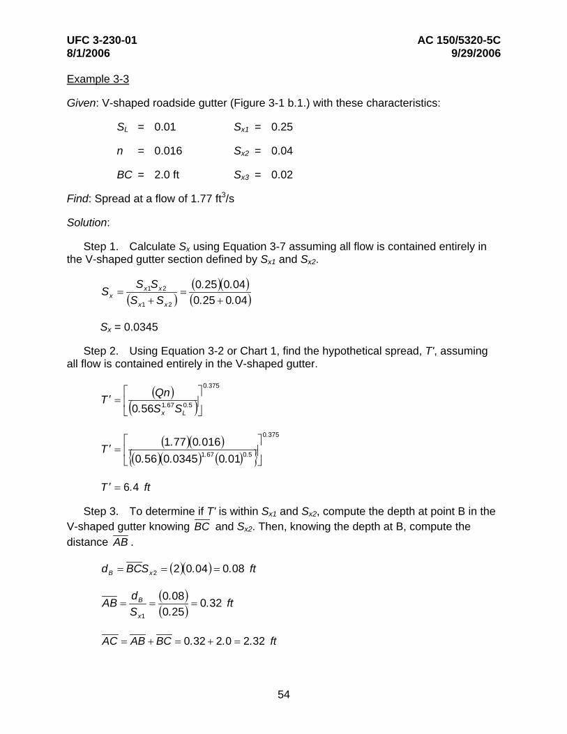
Example 3-3

Given: V-shaped roadside gutter (Figure 3-1 b.1.) with these characteristics:

SL = 0.01 Sx1 = 0.25

n = 0.016 Sx2 = 0.04

BC = 2.0 ft Sx3 = 0.02

Find: Spread at a flow of 1.77 ft3/s

Solution:

Step 1. Calculate Sx using Equation 3-7 assuming all flow is contained entirely in the V-shaped gutter section defined by Sx1 and Sx2.

Sx1Sx2 (0.25)( 0.04)S = = x (Sx1 + Sx2 ) (0.25 + 0.04)

Sx = 0.0345

Step 2. Using Equation 3-2 or Chart 1, find the hypothetical spread, T', assuming all flow is contained entirely in the V-shaped gutter.

⎡ (Qn) ⎤0.375

T ′ = ⎢⎣(0.56Sx

1.67SL 0.5 )⎥⎦

⎡ (1.77)( 0.016) ⎤0.375

T ′ = ⎢{(0.56)( 0.0345)1.67 (0.01)0.5 }⎥ ⎣ ⎦

T ′ = 6.4 ft

Step 3. To determine if T' is within Sx1 and Sx2, compute the depth at point B in the V-shaped gutter knowing BC and Sx2. Then, knowing the depth at B, compute the distance AB .

dB = BCSx2 = (2)(0.04) = 0.08 ft

dB (0.08)AB = = = 0.32 ft Sx1 (0.25)

AC = AB + BC = 0.32 + 2.0 = 2.32 ft

54

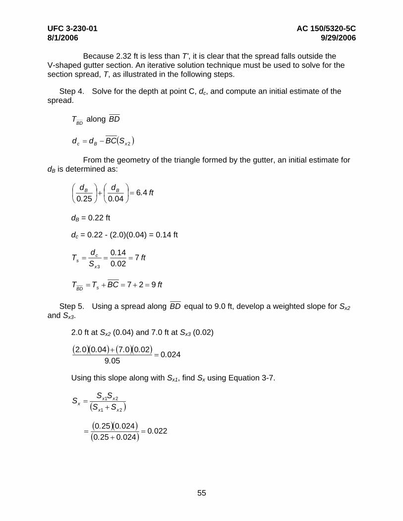
UFC 3-230-01 AC 150/5320-5C 8/1/2006 9/29/2006

Because 2.32 ft is less than T', it is clear that the spread falls outside the V-shaped gutter section. An iterative solution technique must be used to solve for the section spread, T, as illustrated in the following steps.

Step 4. Solve for the depth at point C, dc, and compute an initial estimate of the spread.

T along BDBD

dc = dB − BC(Sx2 )

From the geometry of the triangle formed by the gutter, an initial estimate for dB is determined as:

⎛ dB ⎞ ⎛ dB ⎞⎜ ⎟ + ⎜ ⎟ = 6.4 ft ⎝ 0.25 ⎠ ⎝ 0.04 ⎠

dB = 0.22 ft

dc = 0.22 - (2.0)(0.04) = 0.14 ft

dc 0.14T = = = 7 fts Sx3 0.02

T = T + BC = 7 + 2 = 9 ftBD s

Step 5. Using a spread along BD equal to 9.0 ft, develop a weighted slope for Sx2 and Sx3.

2.0 ft at Sx2 (0.04) and 7.0 ft at Sx3 (0.02)

( . )( . + 7.0)( 0.02 = 0.024

2 0 0 04) ( ) 9.05

Using this slope along with Sx1, find Sx using Equation 3-7.

S SS = x1 x2x (Sx1 + Sx2 )

(0.25)( 0.024)= = 0.022(0.25 + 0.024)

55

UFC 3-230-01 AC 150/5320-5C 8/1/2006 9/29/2006

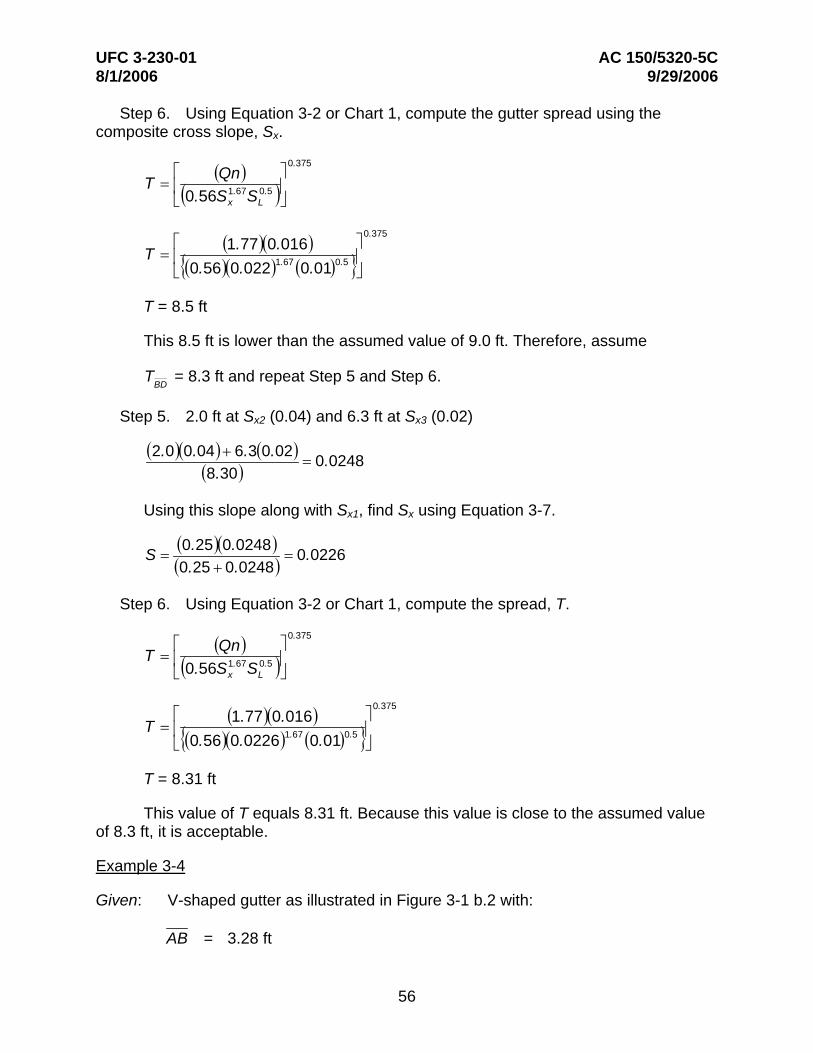
Step 6. Using Equation 3-2 or Chart 1, compute the gutter spread using the composite cross slope, Sx.

⎡ (Qn) ⎤0.375

T = ⎢(0.56S1.67S 0.5 )⎥ ⎣ x L ⎦

⎡ (1.77)( 0.016) ⎤0.375

T = ⎢{(0.56)( 0.022)1.67 (0.01)0.5 }⎥ ⎣ ⎦

T = 8.5 ft

This 8.5 ft is lower than the assumed value of 9.0 ft. Therefore, assume

T = 8.3 ft and repeat Step 5 and Step 6.BD

Step 5. 2.0 ft at Sx2 (0.04) and 6.3 ft at Sx3 (0.02)

(2.0)( 0.04)+ 6.3(0.02)= 0.0248(8.30)

Using this slope along with Sx1, find Sx using Equation 3-7.

(0.25)( 0.0248)S = = 0.0226(0.25 + 0.0248)

Step 6. Using Equation 3-2 or Chart 1, compute the spread, T.

⎡ (Qn) ⎤0.375

T = ⎢ 1.67 0.5 ⎥⎣(0.56Sx SL )⎦

⎡ (1.77)( 0.016) ⎤0.375

T = ⎢{(0.56)( 0.0226)1.67 (0.01)0.5 }⎥ ⎣ ⎦

T = 8.31 ft

This value of T equals 8.31 ft. Because this value is close to the assumed value of 8.3 ft, it is acceptable.

Example 3-4

Given: V-shaped gutter as illustrated in Figure 3-1 b.2 with:

AB = 3.28 ft

56

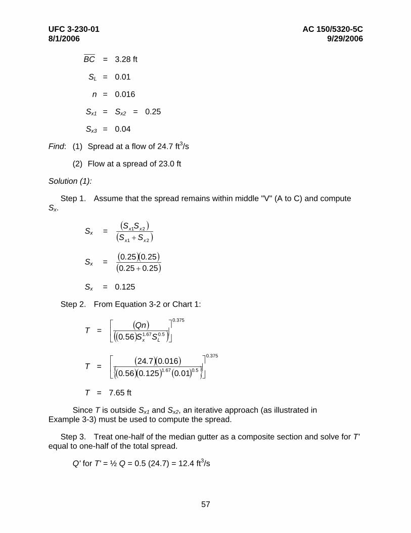
UFC 3-230-01 AC 150/5320-5C 8/1/2006 9/29/2006

BC = 3.28 ft

SL = 0.01

n = 0.016

Sx1 = Sx2 = 0.25

Sx3 = 0.04

Find: (1) Spread at a flow of 24.7 ft3/s

(2) Flow at a spread of 23.0 ft

Solution (1):

Step 1. Assume that the spread remains within middle "V" (A to C) and compute Sx.

(Sx1Sx2 )Sx = (Sx1 +Sx2 )

(0.25)( 0.25)Sx = (0.25 + 0.25)

Sx = 0.125

Step 2. From Equation 3-2 or Chart 1:

⎡ (Qn) ⎤0.375

T = ⎢((0.56)S1.67S0.5 )⎥⎣ x L ⎦

⎡ (24.7)( 0.016) ⎤0.375

T = ⎢⎣{(0.56)( 0.125)1.67 (0.01)0.5 }⎥⎦

T = 7.65 ft

Since T is outside Sx1 and Sx2, an iterative approach (as illustrated in Example 3-3) must be used to compute the spread.

Step 3. Treat one-half of the median gutter as a composite section and solve for T' equal to one-half of the total spread.

Q' for T' = ½ Q = 0.5 (24.7) = 12.4 ft3/s

57

UFC 3-230-01 AC 150/5320-5C 8/1/2006 9/29/2006

Step 4. Try Q's = 1.8 ft3/s

Q'w = Q' - Q's = 12.4 - 1.8 = 10.6 ft3/s

Step 5. Using Equation 3-4 or Chart 2, determine the W/T' ratio.

Qw ′ 10.6E' = = = 0.85o Q′ 12.4

Sw Sx2 0.25 = = = 6.25

Sx Sx3 0.04

W/T' = 0.33 from Chart 2

Step 6. Compute the spread based on the assumed Q'.

W 3.28T ′ = = = 9.94 ft ⎛W ⎞ 0.22⎜ ⎟ ⎝ T ′ ⎠

Step 7. Compute Ts based on the assumed Q's.

Ts = T' - W = 9.94 - 3.28 = 6.66 ft

Step 8. Use Equation 3-2 or Chart 1 to determine Q's for Ts.

Q'sn = (0.56)Sx 1.

367SL

0.5Ts 2.67 = (0.56)(0.04)1.67 (0.01)0.5 (6.66)2.67

Q'sn = 0.041

Q's = 0.041 = 2.56 ft3/s0.016

Step 9. Check the computed Q's with the assumed Q's.

Q's assumed = 1.8 < 2.56 = Q's computed; therefore, try a new assumed Q's and repeat Steps 4 through 9.

Assume Q's = 0.04

Q'w = 12.0 ft3/s

E'o = 0.97

Sw = 6.25 Sx

58

UFC 3-230-01 AC 150/5320-5C 8/1/2006 9/29/2006

W = 0.50 from Chart 2 T ′

T' = 6.56 ft

Ts = 1.0 ft

Qsn = 0.0062

Qs = 0.39 ft3/s

Qs computed = 0.39. This is close to 0.40 = Qs assumed; therefore, the solution is acceptable.

T = 2 T' = 2 (6.56) = 13.12 ft

Solution (2):

Analyze in half-section using composite section techniques. Double the computed half-width flow rate to get the total discharge:

Step 1. Compute half-section top width

T 23T' = = = 11.5 ft2 2

Ts = T' - 3.28 = 8.22 ft

Step 2. From Equation 3-2 or Chart 1, determine Q.

1.67 0.5 2.67Qsn = (0.56)Sx SL Ts

Qsn = (0.56)( 0.04)1.67 (0.01)0.5 (8.22)2.67

Qsn = 0.073

Qs = 0.073 = 4.56 ft3/s0.016

Step 3. Determine the flow in half-section using Equation 3-4 or Chart 2.

T' 11.5= = 3.51 W 3.28

Sw 0.25= = 6.25 S 0.04x

59

UFC 3-230-01 8/1/2006

AC 150/5320-5C 9/29/2006

1 ⎧ ⎡ ⎫⎤

(1 1(

Q' = 24.5 ft3/s

Q = 2 Q' = 2 (24.5) = 49 ft3/s

3-4.4 Flow in Sag Vertical Curves. As gutter flow approaches the low point in a sag vertical curve, the flow can exceed the allowable design spread values as a result of the continually decreasing gutter slope. The spread in these areas should be checked to ensure that it remains within allowable limits. If the computed spread exceeds design values, additional inlets should be provided to reduce the flow as it approaches the low point. Sag vertical curves and measures for reducing spread are discussed further in section 3-5.5.

3-4.5 Gutter Flow Time. The flow time in gutters is an important component of the time of concentration for the contributing drainage area to an inlet. To find the gutter flow component of the time of concentration, a method for estimating the average velocity in a reach of gutter is needed. The velocity in a gutter varies with the flow rate, and the flow rate varies with the distance along the gutter, i.e., both the velocity and flow rate in a gutter are spatially varied. The time of flow can be estimated by use of an average velocity obtained by integration of Manning's equation for the gutter section

⎜ ⎟1

1

⎫⎤

6 25.1 6.25

3.5

⎞⎟⎠

((

(

⎡⎧ ⎪⎪⎨

⎪⎪⎬⎪ ⎪⎭

⎪⎪⎪⎪ ⎪⎪⎬

⎥ ⎥ ⎥ ⎥ ⎥⎦

1

0.814)

⎪ ⎪ ⎪ ⎪ ⎪⎪⎭

⎥⎥⎥⎥⎥⎥⎥⎥⎥⎥⎥⎦

−

−

2.67

2.67

′Qs

Q Q

⎞⎟⎟⎠

4.56

)

′

3.28

Eo = 0.814 = = 1−′Qw

−

)

Sw

x

⎞⎟ ⎟ ⎟ ⎟⎟

⎞⎟ ⎠

⎞⎟⎟⎠

⎠

)

−

⎛⎜⎜⎝

W

1

Sw

xS

S

−

=s

⎛⎜ ⎝

⎛⎜ ⎜ ⎜ ⎜⎜

T⎛⎜⎝

+

0.814)

+

1

1

⎝

⎛⎜⎜⎝

′Q

⎢⎢⎢⎢⎢⎢⎢⎢⎢⎢⎢⎣

⎢ ⎢ ⎢ ⎢ ⎢⎣

+

+

−

1

⎪⎪⎪⎪ ⎪⎪⎨⎪⎪⎪⎪⎪⎪⎩

⎪ ⎪⎩

Eo =

Eo =

Q' =

60

UFC 3-230-01 AC 150/5320-5C 8/1/2006 9/29/2006

with respect to time. The derivation of such a relationship for triangular channels is presented in Appendix C of HEC-22.

Table 3-2 and Chart 4 can be used to determine the average velocity in triangular gutter sections. In Table 3-2, T1 and T2 are the spread at the upstream and downstream ends of the gutter section, respectively. Ta is the spread at the average velocity. Chart 4 in Appendix B is a nomograph to solve Equation 3-13 for the velocity in a triangular channel with known cross slope, gutter slope, and spread.

Table 3-2. Spread at Average Velocity in a Reach of Triangular Gutter

2

1

T T

0 0.1 0.2 0.3 0.4 0.5 0.6 0.7 0.8

T2

Ta 0.65 0.66 0.68 0.70 0.74 0.77 0.82 0.86 0.90

V = 1.11SL

0.5Sx 0.67T 0.67 (3-8)

n

where:

V = velocity in the triangular channel, ft/s

Example 3-5 illustrates the use of Table 3-2 and Chart 4 to determine the average gutter velocity.

Example 3-5

Given: A triangular gutter section with these characteristics:

T1 = 3.28 ft

T2 = 9.84 ft

SL = 0.03 ft/ft

Sx = 0.02 ft/ft

n = 0.016

Inlet spacing is anticipated to be 330 ft.

Find: Time of flow in gutter

61

UFC 3-230-01 AC 150/5320-5C 8/1/2006 9/29/2006

Solution:

Step 1. Compute the upstream to downstream spread ratio.

T 3.281 = = 0.33 T2 9.84

Step 2. Determine the spread at average velocity, interpolating between values in Table 3-2.

(0.30 − 0.33) = X (0.3 − 0.4) (0.74 − 0.70)

X = 0.01

Ta = 7.65 ftT 2

= 0.71

Ta = (0.71)(9.84) = 6.99 ft

Step 3. Using Equation 3-8 or Chart 4, determine the average velocity.

1.11 0.5 0.67 0.67Va = SL Sx Tn

Va = ⎡⎢

1.11 ⎤⎥(0.03)0.5 (0.02)0.67 (6.99)0.67

⎣(0.016)⎦

Va = 3.21 ft/s

Step 4. Compute the travel time in the gutter.

Tti = L/V = (330)/(3.21/(60) = 1.7 min

3-5 DRAINAGE INLET DESIGN. The hydraulic capacity of a storm drain inlet depends upon its geometry as well as the characteristics of the gutter flow. Inlet capacity governs both the rate of water removal from the gutter and the amount of water that can enter the storm drainage system. Inadequate inlet capacity or poor inlet location may cause flooding on the roadway resulting in a hazard to the traveling public.

62

UFC 3-230-01 AC 150/5320-5C 8/1/2006 9/29/2006

3-5.1 Inlet Types. Storm drain inlets are used to collect runoff and discharge it to an underground storm drainage system. Inlets are typically located in gutter sections, paved medians, and roadside and median ditches. Inlets used for the drainage of highway surfaces can be divided into four classes:

Grate inlets

Curb-opening inlets

Combination inlets

Continuous inlets

Grate inlets consist of an opening in the gutter or ditch covered by a grate. Curb-opening inlets are vertical openings in the curb covered by a top slab. Slotted inlets, a form of continuous inlet, consist of a pipe cut along the longitudinal axis with bars perpendicular to the opening to maintain the slotted opening. Combination inlets consist of both a curb-opening inlet and a grate inlet placed in a side-by-side configuration, but the curb opening may be located in part upstream of the grate. Figure 3-3 illustrates each class of inlets. Continuous inlets may also be used with grates, and each type of inlet may be installed with or without a depression of the gutter.

Figure 3-3. Classes of Storm Drain Inlets

a. Grate b. Curb-opening Inleta. Grate b. Curb-opening Inlet

c. Combination Inlet d. Slotted Drain Inletc. Combination Inlet d. Slotted Drain Inlet

63

UFC 3-230-01 AC 150/5320-5C 8/1/2006 9/29/2006

3-5.2 Characteristics and Uses of Inlets

3-5.2.1 Grate Inlets. As a class, grate inlets perform satisfactorily over a wide range of gutter grades. Grate inlets generally lose capacity with increase in grade, but to a lesser degree than curb-opening inlets. The principal advantage of grate inlets is that they are installed along the roadway where the water is flowing. Their principal disadvantage is that they may be clogged by floating trash or debris. For safety reasons, preference should be given to grate inlets where out-of-control vehicles might be involved. Additionally, where bicycle traffic occurs, grates should be bicycle safe.

3-5.2.2 Curb-opening Inlets. Curb-opening inlets are most effective on flatter slopes, in sags, and with flows that typically carry significant amounts of floating debris. The interception capacity of curb-opening inlets decreases as the gutter grade steepens. Consequently, the use of curb-opening inlets is recommended in sags and on grades less than 3 percent. Of course, they are bicycle safe as well.

3-5.2.3 Combination Inlets. Combination inlets provide the advantages of both curb-opening and grate inlets. This combination results in a high capacity inlet that offers the advantages of both grate and curb-opening inlets. When the curb-opening precedes the grate in a "sweeper" configuration, the curb-opening inlet acts as a trash interceptor during the initial phases of a storm. Used in a sag configuration, the sweeper inlet can have a curb opening on both sides of the grate. A complete discussion of combination inlets can be found in Chapter 4 of HEC-22.

3-5.2.4 Continuous Inlets. Continuous inlets can be used in areas where it is necessary to intercept sheet flow before it crosses onto a section of roadway. Their principal advantage is their ability to intercept flow over a wide section. A form of continuous inlet, slotted inlets are very susceptible to clogging from sediments and debris and are not recommended for use in environments where significant sediment or debris loads may be present. Continuous inlets on a longitudinal grade do have the same hydraulic capacity as curb openings when debris is not a factor. A complete discussion of continuous inlets can be found in Chapter 4 of HEC-22.

3-5.3 Inlet Capacity. Inlet interception capacity has been investigated by several agencies and manufacturers of grates. Hydraulic tests on grate inlets and slotted inlets included in this document were conducted by the Bureau of Reclamation for the FHWA. Four of the grates selected for testing were rated highest in bicycle safety tests, three have designs and bar spacing similar to those proven bicycle safe, and a parallel bar grate was used as a standard with which to compare the performance of others.

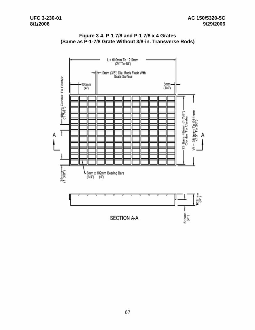
Figures 3-4 through 3-9 show the inlet grates for which design procedures were developed. For ease in identification, the following terms have been adopted:

P-1-7/8 Parallel bar grate with bar spacing 1.875 in. on center (Figure 3-4).

64

UFC 3-230-01 AC 150/5320-5C 8/1/2006 9/29/2006

P-1-7/8 x 4 Parallel bar grate with bar spacing 1.875 in. on center and 0.375-in. diameter lateral rods spaced at 4 in. on center (Figure 3-4).

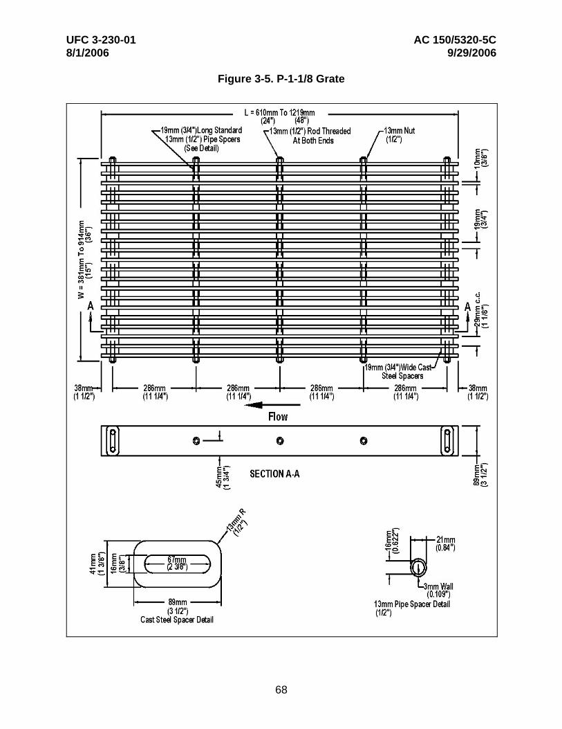
P-1-1/8 Parallel bar grate with 1.125 in. on center bar spacing (Figure 3-5)

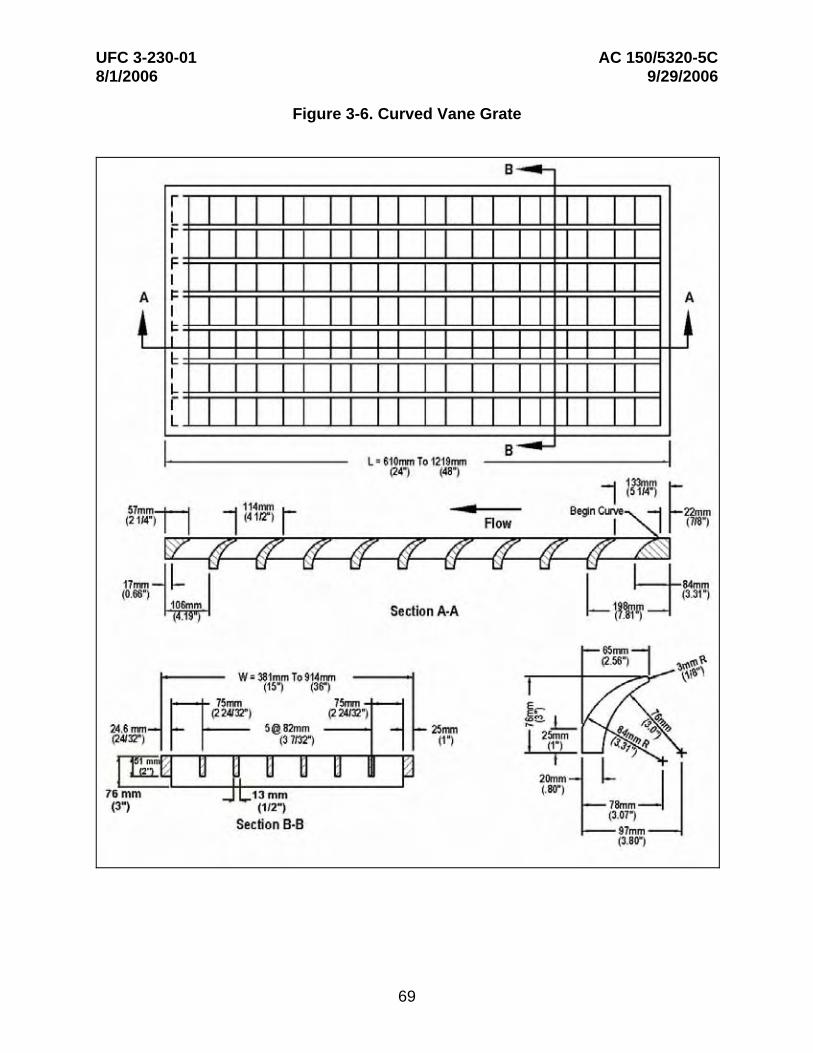
Curved Vane Curved vane grate with 3.25 in. longitudinal bar and 4.25 in. transverse bar spacing on center (Figure 3-6).

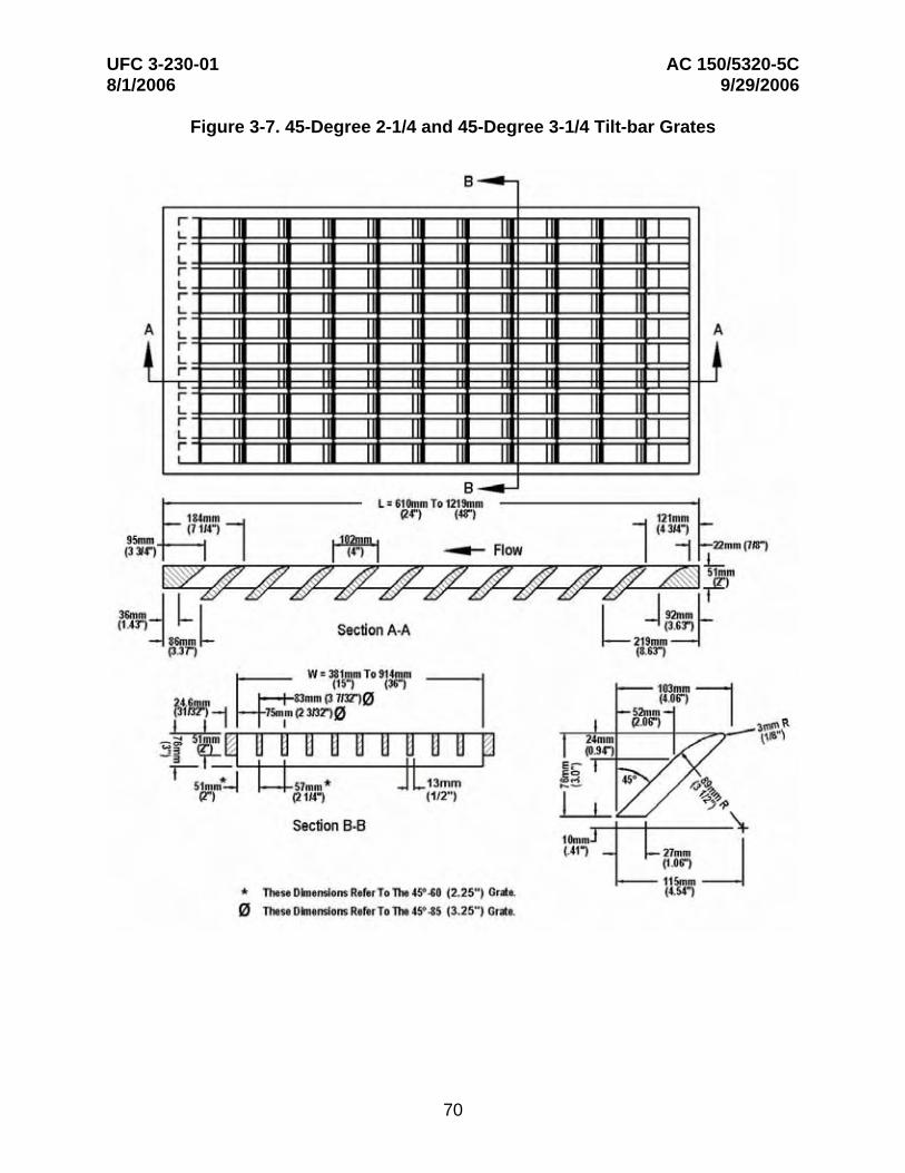
45°- 2-1/4 45-degree tilt-bar grate with 2.25 in. longitudinal bar and 4 in. Tilt Bar transverse bar spacing on center (Figure 3-7).

45°- 3-1/4 45-degree tilt-bar grate with 3.25 in. longitudinal bar and 4 in. Tilt Bar transverse bar spacing on center (Figure 3-7).

30°- 3-1/4 30-degree tilt-bar grate with 3.25 in. longitudinal bar and 4 in. Tilt Bar transverse bar spacing on center (Figure 3-8).

Reticuline "Honeycomb" pattern of lateral bars and longitudinal bearing bars (Figure 3-9).

3-5.3.1 Factors Affecting Inlet Interception Capacity and Efficiency on Continuous Grades. Inlet interception capacity, Qi is the flow intercepted by an inlet under a given set of conditions. The efficiency of an inlet, E, is the percent of total flow that the inlet will intercept for those conditions. The efficiency of an inlet changes with changes in cross slope, longitudinal slope, total gutter flow, and, to a lesser extent, pavement roughness. In mathematical form, efficiency, E, is defined by Equation 3-9:

E = QQ

i (3-9)

where:

E = inlet efficiency

Q = total gutter flow, ft3/s

Qi = intercepted flow, ft3/s

Flow that is not intercepted by an inlet is termed carryover or bypass and is defined by Equation 3-10:

Qb = Q − Qi (3-10)

65

UFC 3-230-01 AC 150/5320-5C 8/1/2006 9/29/2006

where:

Qb = bypass flow, ft3/s

3-5.3.1.1 The interception capacity of all inlet configurations increases with increasing flow rates, and inlet efficiency generally decreases with increasing flow rates. Factors affecting gutter flow also affect inlet interception capacity. The depth of water next to the curb is the major factor in the interception capacity of both grate inlets and curb-opening inlets. The interception capacity of a grate inlet depends on the amount of water flowing over the grate, the size and configuration of the grate, and the velocity of flow in the gutter. The efficiency of a grate is dependent on the same factors and total flow in the gutter.

66

UFC 3-230-01 AC 150/5320-5C 8/1/2006 9/29/2006

Figure 3-4. P-1-7/8 and P-1-7/8 x 4 Grates (Same as P-1-7/8 Grate Without 3/8-in. Transverse Rods)

67

UFC 3-230-01 AC 150/5320-5C 8/1/2006 9/29/2006

Figure 3-5. P-1-1/8 Grate

68

UFC 3-230-01 AC 150/5320-5C 8/1/2006 9/29/2006

Figure 3-6. Curved Vane Grate

69

UFC 3-230-01 AC 150/5320-5C 8/1/2006 9/29/2006

Figure 3-7. 45-Degree 2-1/4 and 45-Degree 3-1/4 Tilt-bar Grates

70

UFC 3-230-01 AC 150/5320-5C 8/1/2006 9/29/2006

Figure 3-8. 30-Degree 3-1/4 Tilt-bar Grates

3-5.3.1.2 Interception capacity of a curb-opening inlet is largely dependent on flow depth at the curb and curb opening length. Flow depth at the curb and consequently, curb-opening inlet interception capacity and efficiency, is increased by the use of a local gutter depression at the curb opening or a continuously depressed gutter to increase the proportion of the total flow adjacent to the curb. Top slab supports placed flush with the curb line can substantially reduce the interception capacity of curb openings. Tests have shown that such supports reduce the effectiveness of openings downstream of the

71

UFC 3-230-01 AC 150/5320-5C 8/1/2006 9/29/2006

support by as much as 50 percent and, if debris is caught at the support, interception by the downstream portion of the opening may be reduced to near zero. If intermediate top slab supports are used, they should be recessed several inches from the curb line and rounded in shape.

Figure 3-9. Reticuline Grate

3-5.3.1.3 Slotted inlets function in essentially the same manner as curb-opening inlets, i.e., as weirs with flow entering from the side. Interception capacity is dependent on flow depth and inlet length. Efficiency is dependent on flow depth, inlet length, and total gutter flow.

3-5.3.1.4 The interception capacity of an equal length combination inlet consisting of a grate placed alongside a curb opening on a grade does not differ materially from that of a grate only. Interception capacity and efficiency are dependent on the same factors that affect grate capacity and efficiency. A combination inlet consisting of a curb-opening inlet placed upstream of a grate inlet has a capacity equal to that of the curb-opening length upstream of the grate plus that of the grate, taking into account the reduced spread and depth of flow over the grate because of the interception by the curb opening. This inlet configuration has the added advantage of intercepting debris that might otherwise clog the grate and deflect water away from the inlet.

72

UFC 3-230-01 AC 150/5320-5C 8/1/2006 9/29/2006

3-5.4 Interception Capacity of Inlets on Grade. Section 3-5.3.1 examines the factors that influence the interception capacity of inlets on grade. This section (3-5.4) introduces the design charts for inlets on grade (Appendix B) and procedures for using the charts for the various inlet configurations. Remember that for locally depressed inlets, the quantity of flow reaching the inlet would be dependent on the upstream gutter section geometry and not the depressed section geometry.

Charts for grate inlet interception are presented in Appendix B. The chart for frontal flow interception is based on test results that show that grates intercept all of the frontal flow until a velocity is reached at which water begins to splash over the grate. At velocities greater than "splash-over" velocity, grate efficiency in intercepting frontal flow is diminished. Grates also intercept a portion of the flow along the length of the grate, or the side flow. A chart is provided to determine side-flow interception.

One set of charts is provided for slotted inlets and curb-opening inlets because these inlets are both side-flow weirs. The equation developed for determining the length of inlet required for total interception fits the test data for both types of inlets.

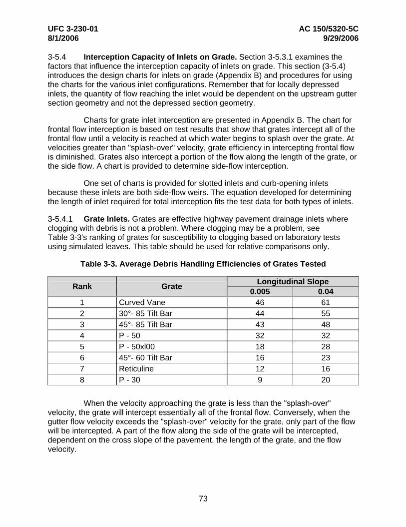
3-5.4.1 Grate Inlets. Grates are effective highway pavement drainage inlets where clogging with debris is not a problem. Where clogging may be a problem, see Table 3-3's ranking of grates for susceptibility to clogging based on laboratory tests using simulated leaves. This table should be used for relative comparisons only.

Table 3-3. Average Debris Handling Efficiencies of Grates Tested

Rank Grate Longitudinal Slope 0.005 0.04

1 Curved Vane 46 61 2 30°- 85 Tilt Bar 44 55 3 45°- 85 Tilt Bar 43 48 4 P - 50 32 32 5 P - 50xl00 18 28 6 45°- 60 Tilt Bar 16 23 7 Reticuline 12 16 8 P - 30 9 20

When the velocity approaching the grate is less than the "splash-over" velocity, the grate will intercept essentially all of the frontal flow. Conversely, when the gutter flow velocity exceeds the "splash-over" velocity for the grate, only part of the flow will be intercepted. A part of the flow along the side of the grate will be intercepted, dependent on the cross slope of the pavement, the length of the grate, and the flow velocity.

73

UFC 3-230-01 AC 150/5320-5C 8/1/2006 9/29/2006

3-5.4.1.1 The ratio of frontal flow to total gutter flow, Eo, for a uniform cross slope is expressed by Equation 3-11:

Eo =Qw = 1− ⎜

⎛1− W ⎞

⎟ 2.67

(3-11)Q ⎝ T ⎠

where:

Q = total gutter flow, ft3/s

Qw = flow in width, W, ft3/s

W = width of depressed gutter or grate, ft

T = total spread of water, ft

Example 3-2 and Chart 2 provide solutions of Eo for either uniform cross slopes or composite gutter sections.

3-5.4.1.2 The ratio of side flow, Qs, to total gutter flow is:

Qs = 1− Qw = 1− E (3-12)

Q Q o

3-5.4.1.3 The ratio of frontal flow intercepted to total frontal flow, Rf, is expressed by Equation 3-13:

Rf = 1− 0.09(V −Vo ) (3-13)

where:

V = velocity of flow in the gutter, ft/s

Vo = gutter velocity where splash-over first occurs, ft/s

(NOTE: Rf cannot exceed 1.0.)

This ratio is equivalent to frontal flow interception efficiency. Chart 5 provides a solution for Equation 3-13 that takes into account grate length, bar configuration, and gutter velocity at which splash-over occurs. The average gutter velocity (total gutter flow divided by the area of flow) is needed to use Chart 5. This velocity can also be obtained from Chart 4.

3-5.4.1.4 The ratio of side flow intercepted to total side flow, Rs, or side flow interception efficiency, is expressed by Equation 3-14. Chart 6 in Appendix B provides a solution to Equation 3-14.

74

UFC 3-230-01 AC 150/5320-5C 8/1/2006 9/29/2006

1R = (3-14)s ⎛ 0.15V 1.8 ⎞ ⎜⎜1+ 2.3 ⎟⎟ ⎝ SxL ⎠

A deficiency in developing empirical equations and charts from experimental data is evident in Chart 6. The fact that a grate will intercept all or almost all of the side flow where the velocity is low and the spread only slightly exceeds the grate width is not reflected in the chart. Error due to this deficiency is very small. In fact, where velocities are high, side flow interception may be neglected without significant error.

3-5.4.1.5 The efficiency, E, of a grate is expressed as in Equation 3-15:

E = Rf Eo + Rs (1− Eo ) (3-15)

The first term on the right side of Equation 3-15 is the ratio of intercepted frontal flow to total gutter flow, and the second term is the ratio of intercepted side flow to total side flow. The second term is insignificant with high velocities and short grates.

3-5.4.1.6 It is important to recognize that the frontal flow to total gutter flow ratio, Eo, for composite gutter sections assumes by definition a frontal flow width equal to the depressed gutter section width. The use of this ratio when determining a grate's efficiency requires that the grate width be equal to the width of the depressed gutter section, W. If a grate having a width less than W is specified, the gutter flow ratio, Eo, must be modified to accurately evaluate the grate's efficiency. Because an average velocity has been assumed for the entire width of gutter flow, the grate's frontal flow ratio, Eo, can be calculated by multiplying Eo by a flow area ratio. The area ratio is defined as the gutter flow area in a width equal to the grate width divided by the total flow area in the depressed gutter section. This adjustment is represented in Equation 3-15a:

⎛ A′ ⎞wEo ′ = Eo ⎜⎜ A ⎟⎟ (3-15a)

⎝ w ⎠

where:

E'o = adjusted frontal flow area ratio for grates in composite cross sections

A'w = gutter flow area in a width equal to the grate width, ft2

Aw = flow area in depressed gutter width, ft2

3-5.4.1.7 The interception capacity of a grate inlet on grade is equal to the efficiency of the grate multiplied by the total gutter flow as represented in Equation 3-16. Note that E'o should be used in place of Eo in Equation 3-16 when appropriate.

Qi = EQ = Q[Rf Eo + Rs (1− Eo )] (3-16)

75

UFC 3-230-01 AC 150/5320-5C 8/1/2006 9/29/2006

3-5.4.1.8 The use of Chart 5 and Chart 6 is illustrated in the Examples 3-6 and 3-7.

Example 3-6

Given: The gutter section from Example 3-2 (illustrated in Figure 3-1 a.2) with:

T = 8.2 ft

SL = 0.010

Sx = 0.020

W = 2.0 ft

n = 0.016

Continuous gutter depression, a = 2 in. or 0.167 ft

Find: The interception capacity of a curved vane grate 2 ft by 2 ft

Solution: From Example 3-2:

Sw = 0.103 ft/ft

Eo = 0.70

Q = 2.3 ft3/s

Step 1. Compute the average gutter velocity.

Q 2.3V = = A A

A = 0.5 T2Sx + 0.5 a W

A = 0.5(8.2)2(0.2) + 0.5(0.167)(2.0)

A = 0.84 ft2

2.3V = = 2.74 ft/s0.84

Step 2. Determine the frontal flow efficiency using Chart 5.

Rf = 1.0

76

UFC 3-230-01 AC 150/5320-5C 8/1/2006 9/29/2006

Step 3. Determine the side flow efficiency using Equation 3-14 or Chart 6.

1Rs = 1.8⎡1+ (0.15V )⎤

⎢ 2.3 ⎥ ⎣ (S L )x ⎦

1Rs = ⎡1+ (0.15)( 2.74)1.8 ⎤ ⎢ ⎥ ⎣ (0.02)( 2.0)2.3

⎦

Rs = 0.10

Step 4. Compute the interception capacity using Equation 3-16.

Qi = Q [RfEo + Rs(1-Eo)]

Qi = (2.3) [(1.0(0.70) + (0.10)(1-0.70)]

Qi = 1.68 ft3/s

Example 3-7

Given: The gutter section illustrated in Figure 3-1 a.1 with:

T = 9.84 ft

SL = 0.04 ft/ft

Sx = 0.025 ft/ft

n = 0.016

Bicycle traffic not permitted.

Find: The interception capacity of the following grates:

a. P-50: 2.0 ft x 2.0 ft

b. Reticuline: 2.0 ft x 2.0 ft

c. Grates in a. and b. with a length of 4.0 ft

Solution:

Step 1. Using Equation 3-2 or Chart 1, determine Q.

77

UFC 3-230-01 AC 150/5320-5C 8/1/2006 9/29/2006

0.56⎛⎜⎝

1.67 0.5 2.67TSQ = Lx n S⎞⎟⎠

).0.016 (⎧

⎨⎩

0.025(⎫⎬⎭

56

Q = 6.62 ft3/s

Step 2. Determine Eo from Equation 3-4 or Chart 2.

W 2.0 = T 9.84

= 0.2

QwEo =

(

Q

)()( )2.67Q 1.67 0.5= 0.04 9.84)

2.67W⎞⎟⎠

1 ⎛1−−Eo =

= 1 - (1-0.2)2.67

Eo = 0.45

⎜⎝

Step 3. Using Equation 3-8 or Chart 4, compute the gutter flow velocity.

T

1.11⎛⎜⎝

))

⎞⎟⎠S 0.5 0.67 0.67TV = SL x n

()()((

V = 5.4 ft/s

Step 4. Using Equation 3-13 or Chart 5, determine the frontal flow efficiency for each grate.

Using Equation 3-14 or Chart 6, determine the side flow efficiency for each grate.

Using Equation 3-16, compute the interception capacity of each grate.

Table 3-4 summarizes the results.

⎧⎨⎩

(⎫⎬⎭

0.04 )0.671.11V 0.5 0.67 = 0.025 9.840.016

78

UFC 3-230-01 8/1/2006

AC 150/5320-5C 9/29/2006

Table 3-4. Grate Efficiency and Capacity Summary

Grate Size (width by length)

Frontal Flow Efficiency, Rf

Side Flow Efficiency, Rs

Interception Capacity, Qi

P – 1-7/8 2.0 ft by 2.0 ft 1.0 0.036 3.21 ft3/s Reticuline 2.0 ft by 2.0 ft 0.9 0.036 2.89 ft3/s P – 1-7/8 2.0 ft by 4.0 ft 1.0 0.155 3.63 ft3/s Reticuline 2.0 ft by 4.0 ft 1.0 0.155 3.63 ft3/s NOTE: The P-1-7/8 parallel bar grate will intercept about 14 percent more flow than the reticuline grate, or 48 percent of the total flow as opposed to 42 percent for the reticuline grate. Increasing the length of the grates would not be cost effective because the increase in side flow interception is small.

3-5.4.2 Curb-opening Inlets. Curb-opening inlets are effective in the drainage of highway pavements where flow depth at the curb is sufficient for the inlet to perform efficiently, as discussed in section 3-5.3.1. Curb openings are less susceptible to clogging and offer little interference to traffic operation. They are a viable alternative to grates on flatter grades where grates would be in traffic lanes or would be hazardous for pedestrians or bicyclists.

3-5.4.2.1 Curb opening heights vary in dimension; however, a typical maximum height is approximately 4 to 6 inches. The length of the curb-opening inlet required for total interception of gutter flow on a pavement section with a uniform cross slope is expressed by Equation 3-17:

0.6 0.42 0.3L = (0.6)Q S

⎛⎜⎜

1 ⎞⎟⎟ (3-17)T L

⎝ nSx ⎠

where:

LT = curb opening length required to intercept 100 percent of the gutter flow, ft

SL = longitudinal slope

Q = gutter flow, ft3/s

3-5.4.2.2 The efficiency of curb-opening inlets shorter than the length required for total interception is expressed by Equation 3-18:

1.8⎛ L ⎞E = 1− ⎜⎜1− ⎟⎟ (3-18)⎝ LT ⎠

79

UFC 3-230-01 AC 150/5320-5C 8/1/2006 9/29/2006

where:

L = curb opening length, ft

Chart 7 is a nomograph for the solution of Equation 3-17, and Chart 8 provides a solution to Equation 3-18.

3-5.4.2.3 The length of inlet required for total interception by depressed curb-opening inlets or curb openings in depressed gutter sections can be found by the use of an equivalent cross slope, Se, in Equation 3-17 in place of Sx. Se can be computed using Equation 3-19.

S = S + S′ E (3-19)e x w o

where:

S'w = cross slope of the gutter measured from the cross slope of the pavement, Sx, ft/ft

S'w = [12 aW ], for W in ft, or = Sw - Sx

a = gutter depression, in.

Eo = ratio of flow in the depressed section to total gutter flow determined by the gutter configuration upstream of the inlet

Figure 3-10 shows the depressed curb inlet for Equation 3-19. Eo is the same ratio as used to compute the frontal flow interception of a grate inlet.

Figure 3-10. Depressed Curb-opening Inlet

3-5.4.2.4 As seen from Chart 7, the length of the curb opening required for total interception can be significantly reduced by increasing the cross slope or the equivalent cross slope. The equivalent cross slope can be increased by use of a continuously depressed gutter section or a locally depressed gutter section.

80

UFC 3-230-01 AC 150/5320-5C 8/1/2006 9/29/2006

Using the equivalent cross slope, Se, Equation 3-17 becomes:

0.6 0.42 0.3LT = (0.6)Q SL

⎛⎜⎜

1 ⎞⎟⎟ (3-20)

⎝ nSe ⎠

3-5.4.2.5 Equation 3-18 is applicable with either straight cross slopes or composite cross slopes. Charts 7 and 8 are applicable to depressed curb-opening inlets using Se rather than Sx.

3-5.4.2.6 Equation 3-19 uses the ratio, Eo, in the computation of the equivalent cross slope, Se. Example 3-8a demonstrates the procedure to determine spread and then uses Chart 2 to determine Eo. Example 3-8b demonstrates the use of these relationships to design the length of a curb-opening inlet.

Example 3-8a

Given: A curb-opening inlet with the following characteristics:

SL = 0.014 ft/ft

Sx = 0.02 ft/ft

Q = 1.77 ft3/s

n = 0.016

Find: The interception capacity of the following grates:

(1) Qi for a 9.84 ft curb opening.

(2) Qi for a depressed 9.84 ft curb-opening inlet with a continuously depressed curb section.

a = 1 in.

W = 2 ft

Solution (1):

Step 1. Determine the length of curb opening required for total interception of gutter flow using Equation 3-17 or Chart 7.

0.6 0.42 0.3LT = (0.6)Q SL

⎛⎜⎜

1 ⎞⎟⎟

⎝ nSx ⎠

81

UFC 3-230-01 AC 150/5320-5C 8/1/2006 9/29/2006

0.6 0.42 0.3 ⎛ 1 ⎞LT = (0.6)(1.77) (0.014)

⎝⎜⎜ [(0.016)(0.02)]⎠⎟

⎟

LT = 23.94 ft

Step 2. Compute the curb-opening efficiency using Equation 3-18 or Chart 8.

L 9.84 = = 0.41 LT 23.94

1.8⎛ L ⎞E = 1− ⎜⎜1− ⎟⎟⎝ LT ⎠

.E = 1− (1− 0.41)1 8

E = 0.61

Step 3. Compute the interception capacity.

Qi = E Q

= (0.61)(1.77)

Qi = 1.08 ft3/s

Solution (2):

Step 1. Use Equation 3-4 (Chart 2) and Equation 3-2 (Chart 1) to determine the W/T ratio.

Determine the spread, T (procedure from Example 3-2, Solution 2).

Assume Qs = 0.64 ft3/s

Qw = Q - Qs

= 1.77 - 0.64

= 1.13 ft3/s

QEo = w

Q

1.13 = 1.77

82

UFC 3-230-01 8/1/2006

AC 150/5320-5C 9/29/2006

= 0.64

aSw = Sx +W

0.83= 0.02+2.0

Sw = 0.062

S 0.062=3.1w =

S 0.02x

Use Equation 3-4 or Chart 2 to determine W/T.

W = 0.24T

WT = W⎛⎜⎝

⎞⎟⎠T

2.0 = 0.24

= 8.33 ft

Ts = T - W

= 8.3 - 2.0

= 6.3 ft

Use Equation 3-2 or Chart 1 to obtain Qs.

0.56⎛⎜⎝

)

⎞⎟⎠S1.67 0.5 2.67TQs = SLx s n

()()((

Qs = 0.69 ft3/s, which is close to the Qs assumed value

⎧⎨⎩

(⎫⎬⎭

)0.56 2.67Qs1.67 0.5= 0.02 0.01 6.3)0.016

83

UFC 3-230-01 AC 150/5320-5C 8/1/2006 9/29/2006

Step 2. Determine the efficiency of the curb opening.

Se = Sx + Sw ′ Eo = Sx + ⎜⎛ a

⎟⎞Eo

⎝W ⎠

⎡(0.083)⎤(= 0.02 + ⎢ (2.0) ⎥ 0. / 64)⎣ ⎦

Se = 0.047

Using Equation 3-20 or Chart 7:

0.6 0.42 0.3LT = (0.6)Q SL

⎛⎜⎜

1 ⎞⎟⎟

⎝ nSe ⎠

0.6 0.42 0.3 ⎡ 1 ⎤LT = (0.6)( 1.77) (0.01)

⎣⎢((0.016)( 0.047))⎦⎥

LT = 14.34 ft

Using Equation 3-18 or Chart 8 to obtain curb inlet efficiency:

L 9.84= = 0.69

LT 14.34

1.8⎛ L ⎞E = 1− 1−⎜⎜ LT

⎟⎟⎝ ⎠

.E = 1− (1− 0.69)1 8

E = 0.88

Step 3. Compute curb opening inflow using Equation 3-9.

Qi = Q E

= (1.77)(0.88)

Qi = 1.55 ft3/s

The depressed curb-opening inlet will intercept 1.5 times the flow intercepted by the undepressed curb opening.

84

UFC 3-230-01 AC 150/5320-5C 8/1/2006 9/29/2006

Example 3-8b

Given: From Example 3-6:

SL = 0.01 ft/ft

Sx = 0.02 ft/ft

T = 8.2 ft

Q = 2.26 ft3/s

n = 0.016

W = 2.0 ft

A = 2.0 in

Eo = 0.70

Find: The minimum length of a locally depressed curb-opening inlet required to intercept 100 percent of the gutter flow.

Solution:

Step 1. Compute the composite cross slope for the gutter section using Equation 3-19.

Se = Sx +Sw ′ Eo

⎛ 2 12 ⎞Se = 0.02 + ⎜ ⎟0.60 ⎝ 0.6 ⎠

Se = 0.07

Step 2. Compute the length of curb-opening inlet required from Equation 3-20.

0.6 0.42 0.3LT = (0.6)Q SL

⎛⎜⎜

1 ⎞⎟⎟

⎝ nSe ⎠

0.6 0.42 0.3 ⎡ 1 ⎤LT = (0.6)( 2.26) (0.01)

⎣⎢(0.016)( 0.07)⎦⎥

LT = 12.5 ft

3-5.4.2.7 The use of depressed inlets and combination inlets enhances the interception capacity of the inlet. Example 3-6 determined the interception capacity of a depressed

85

UFC 3-230-01 AC 150/5320-5C 8/1/2006 9/29/2006

curved vane grate, 2 ft by 2 ft; Examples 3-8a and 3-8b for an undepressed curb-opening inlet with a length of 9.8 ft and a depressed curb-opening inlet with a length of 9.8 ft; and Example 3-10 for a combination of 2 ft by 2 ft depressed curve vane grate located at the downstream end of a 9.8-ft-long depressed curb-opening inlet. The geometries of the inlets and the gutter slopes were consistent in the examples, and Table 3-5 summarizes a comparison of the intercepted flow of the various configurations.

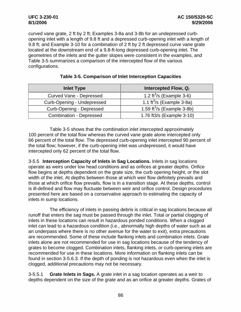
Table 3-5. Comparison of Inlet Interception Capacities

Inlet Type Intercepted Flow, Qi

Curved Vane - Depressed 1.2 ft3/s (Example 3-6) Curb-Opening - Undepressed 1.1 ft3/s (Example 3-8a) Curb-Opening - Depressed 1.59 ft3/s (Example 3-8b) Combination - Depressed 1.76 ft3/s (Example 3-10)

Table 3-5 shows that the combination inlet intercepted approximately 100 percent of the total flow whereas the curved vane grate alone intercepted only 66 percent of the total flow. The depressed curb-opening inlet intercepted 90 percent of the total flow; however, if the curb-opening inlet was undepressed, it would have intercepted only 62 percent of the total flow.

3-5.5 Interception Capacity of Inlets in Sag Locations. Inlets in sag locations operate as weirs under low head conditions and as orifices at greater depths. Orifice flow begins at depths dependent on the grate size, the curb opening height, or the slot width of the inlet. At depths between those at which weir flow definitely prevails and those at which orifice flow prevails, flow is in a transition stage. At these depths, control is ill-defined and flow may fluctuate between weir and orifice control. Design procedures presented here are based on a conservative approach to estimating the capacity of inlets in sump locations.

The efficiency of inlets in passing debris is critical in sag locations because all runoff that enters the sag must be passed through the inlet. Total or partial clogging of inlets in these locations can result in hazardous ponded conditions. When a clogged inlet can lead to a hazardous condition (i.e., abnormally high depths of water such as at an underpass where there is no other avenue for the water to exit), extra precautions are recommended. Some of these include flanking inlets and combination inlets. Grate inlets alone are not recommended for use in sag locations because of the tendency of grates to become clogged. Combination inlets, flanking inlets, or curb-opening inlets are recommended for use in these locations. More information on flanking inlets can be found in section 3-5.6.3. If the depth of ponding is not hazardous even when the inlet is clogged, additional precautions may not be necessary.

3-5.5.1 Grate Inlets in Sags. A grate inlet in a sag location operates as a weir to depths dependent on the size of the grate and as an orifice at greater depths. Grates of

86

UFC 3-230-01 AC 150/5320-5C 8/1/2006 9/29/2006

larger dimension will operate as weirs to greater depths than smaller grates. The capacity of grate inlets operating as weirs is:

Qi =Cw Pd 1.5 (3-21)

where:

P = perimeter of the grate (ft) disregarding the side against the curb

Cw = weir coefficient, 3.0

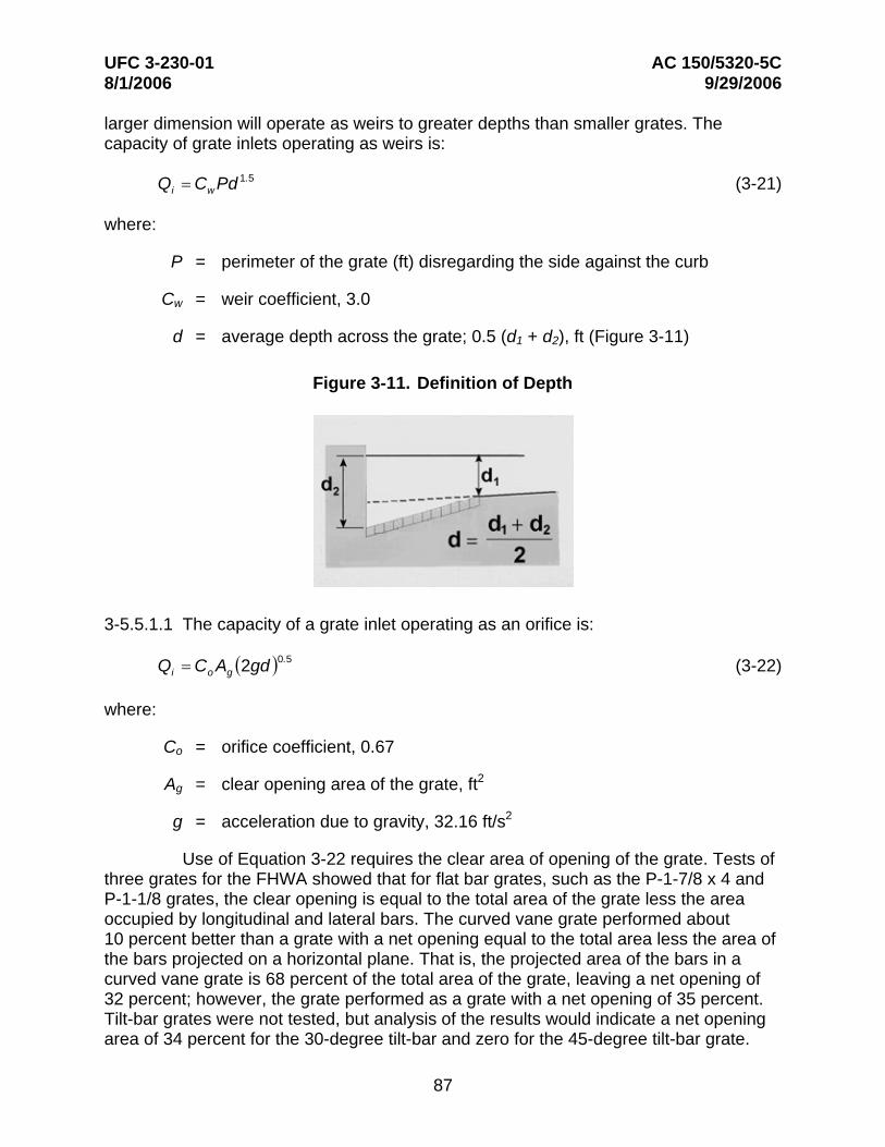
d = average depth across the grate; 0.5 (d1 + d2), ft (Figure 3-11)

Figure 3-11. Definition of Depth

3-5.5.1.1 The capacity of a grate inlet operating as an orifice is:

.Qi =Co Ag (2gd )0 5 (3-22)

where:

Co = orifice coefficient, 0.67

Ag = clear opening area of the grate, ft2

g = acceleration due to gravity, 32.16 ft/s2

Use of Equation 3-22 requires the clear area of opening of the grate. Tests of three grates for the FHWA showed that for flat bar grates, such as the P-1-7/8 x 4 and P-1-1/8 grates, the clear opening is equal to the total area of the grate less the area occupied by longitudinal and lateral bars. The curved vane grate performed about 10 percent better than a grate with a net opening equal to the total area less the area of the bars projected on a horizontal plane. That is, the projected area of the bars in a curved vane grate is 68 percent of the total area of the grate, leaving a net opening of 32 percent; however, the grate performed as a grate with a net opening of 35 percent. Tilt-bar grates were not tested, but analysis of the results would indicate a net opening area of 34 percent for the 30-degree tilt-bar and zero for the 45-degree tilt-bar grate.

87

UFC 3-230-01 AC 150/5320-5C 8/1/2006 9/29/2006

Obviously, the 45-degree tilt-bar grate would have greater than zero capacity. Tilt-bar and curved vane grates are not recommended for sump locations where there is a chance that operation would be as an orifice. Opening ratios for the grates are given on Chart 9 in Appendix B.

3-5.5.1.2 Chart 9 is a plot of Equations 3-21 and 3-22 for various grate sizes. The effects of grate size on the depth at which a grate operates as an orifice is apparent from the chart. Transition from weir to orifice flow results in interception capacity less than that computed by either the weir or the orifice equation. This capacity can be approximated by drawing a curve between the lines representing the perimeter and net area of the grate to be used.

Example 3-9 illustrates use of Equations 3-21 and 3-22 and Chart 9.

Example 3-9

Given: Under design storm conditions, a flow to the sag inlet is 6.71 ft3/s. Also:

Sx = 0.05 ft/ft

n = 0.016

Tallowable = 9.84 ft

Find: The grate size required and depth at curb for the sag inlet assuming 50 percent clogging where the width of the grate, W, is 2.0 ft.

⎛− ⎜⎝

Solution:

Step 1. Determine the required grate perimeter.

Depth at curb, d2:

d2 = T Sx = (9.84)(0.05)

d2 = 0.49 ft

Average depth over grate:

W⎞⎟⎠Swd = d2 2

2.0 (⎞⎟⎠

.05)d = 0.49 2

⎛− ⎜⎝

d = 0.445 ft

88

UFC 3-230-01 AC 150/5320-5C 8/1/2006 9/29/2006

From Equation 3-26 or Chart 9:

QiP = [C d 1.5 ]w

(6.71)P = .[(3.0)( 0.44)1 5 ] P = 7.66 ft

Some assumptions must be made regarding the nature of the clogging in order to compute the capacity of a partially clogged grate. If the area of a grate is 50 percent covered by debris so that the debris-covered portion does not contribute to interception, the effective perimeter will be reduced by a lesser amount than 50 percent. For example, if a 2 ft by 4 ft grate is clogged so that the effective width is 1 ft, then the calculation for the perimeter, P, is P = 1 + 4 +1 = 6 ft, rather than 7.66 ft, the total perimeter, or 3.83 ft, half of the total perimeter. The area of the opening would be reduced by 50 percent and the perimeter by 25 percent. Therefore, assuming 50 percent clogging along the length of the grate, a 4 ft by 4 ft, 2 ft by 6 ft, or a 3 ft by 5 ft grate would meet the requirements of a 7.66 ft perimeter 50 percent clogged.

Assuming 50 percent clogging along the grate length,

Peffective = 8.0 = (0.5)(2) W + L

If W = 2 ft, then L > 5 ft

If W = 3 ft, then L ≥ 5 ft

Select a double 2 ft by 3 ft grate:

Peffective = (0.5)(2)(2.0) + (6)

Peffective = 8 ft

Step 2. Check the depth of flow at the curb using Equation 3-21 or Chart 9.

0.67⎡ Q ⎤

d = ⎢ ⎥⎣(CwP )⎦

0.67⎡ 6.71 ⎤d = ⎢⎣(3.0)( 8.0)⎥⎦

d = 0.43 ft

89

UFC 3-230-01 AC 150/5320-5C 8/1/2006 9/29/2006

Conclusion:

A double 2 ft by 3 ft grate 50 percent clogged is adequate to intercept the design storm flow at a spread that does not exceed design spread; however, the tendency of grate inlets to clog completely warrants consideration of a combination inlet or curb-opening inlet in a sag where ponding can occur, and flanking inlets in long flat vertical curves.

3-5.5.2 Curb-opening Inlets. The capacity of a curb-opening inlet in a sag depends on the water depth at the curb, the curb opening length, and the height of the curb opening. The inlet operates as a weir to depths equal to the curb opening height and as an orifice at depths greater than 1.4 times the opening height. At depths between 1.0 and 1.4 times the opening height, flow is in a transition stage.

3-5.5.2.1 Spread on the pavement is the usual criterion for judging the adequacy of a pavement drainage inlet design. It is also convenient and practical in the laboratory to measure depth at the curb upstream of the inlet at the point of maximum spread on the pavement. Therefore, depth at the curb measurements from experiments coincide with the depth at the curb of interest to designers. The weir coefficient for a curb-opening inlet is less than the usual weir coefficient for several reasons, the most obvious of which is that depth measurements from experimental tests were not taken at the weir, and drawdown occurs between the point where measurements were made and the weir.

3-5.5.2.2 The weir location for a depressed curb-opening inlet is at the edge of the gutter, and the effective weir length is dependent on the width of the depressed gutter and the length of the curb opening. The weir location for a curb-opening inlet that is not depressed is at the lip of the curb opening, and its length is equal to that of the inlet, as shown in Chart 10 of Appendix B.

3-5.5.2.3 The equation for the interception capacity of a depressed curb-opening inlet operating as a weir is:

1.5Qi =Cw (L + 1.8 W ) d (3-23)

where:

Cw = 2.3

L = length of curb opening, ft

W = lateral width of depression, ft

d = depth at curb measured from the normal cross slope, ft, i.e., d = T Sx

3-5.5.2.4 The weir equation is applicable to depths at the curb approximately equal to the height of the opening plus the depth of the depression. Thus, the limitation on the use of Equation 3-23 for a depressed curb-opening inlet is:

90

UFC 3-230-01 AC 150/5320-5C 8/1/2006 9/29/2006

d ≤ h + a (3-24)

12

where:

h = height of curb-opening inlet, ft

a = depth of depression, in.

3-5.5.2.5 Experiments have not been conducted for curb-opening inlets with a continuously depressed gutter, but it is reasonable to expect that the effective weir length would be as great as that for an inlet in a local depression. Use of Equation 3-23 will yield conservative estimates of the interception capacity.

3-5.5.2.6 The weir equation for curb-opening inlets without depression becomes:

Qi =Cw L d 1.5 (3-25)

Without depression of the gutter section, the weir coefficient, Cw, becomes 3.0. The depth limitation for operation as a weir becomes d ≤ h.

3-5.5.2.7 At curb-opening lengths greater than 12 ft, Equation 3-25 for non-depressed inlets produces intercepted flows that exceed the values for depressed inlets computed using Equation 3-23. Since depressed inlets will perform at least as well as non-depressed inlets of the same length, Equation 3-25 should be used for all curb-opening inlets with lengths greater than 12 ft.

3-5.5.2.8 Curb-opening inlets operate as orifices at depths greater than approximately 1.4 times the opening height. The interception capacity can be computed by Equation 3-26a and Equation 3-26b. These equations are applicable to depressed and undepressed curb-opening inlets. The depth at the inlet includes any gutter depression.

.Qi = Coh L (2 g do )0 5 (3-26a)

or

0.5

Qi =Co Ag ⎢⎡2g⎜⎛di −

h ⎟⎞⎥⎤ (3-26b)

⎣ ⎝ 2 ⎠⎦

where:

Co = orifice coefficient (0.67)

do = effective head on the center of the orifice throat, ft

L = length of orifice opening, ft

91

UFC 3-230-01 AC 150/5320-5C 8/1/2006 9/29/2006

Ag = clear area of opening, ft2

di = depth at lip of curb opening, ft

h = height of curb-opening orifice, ft

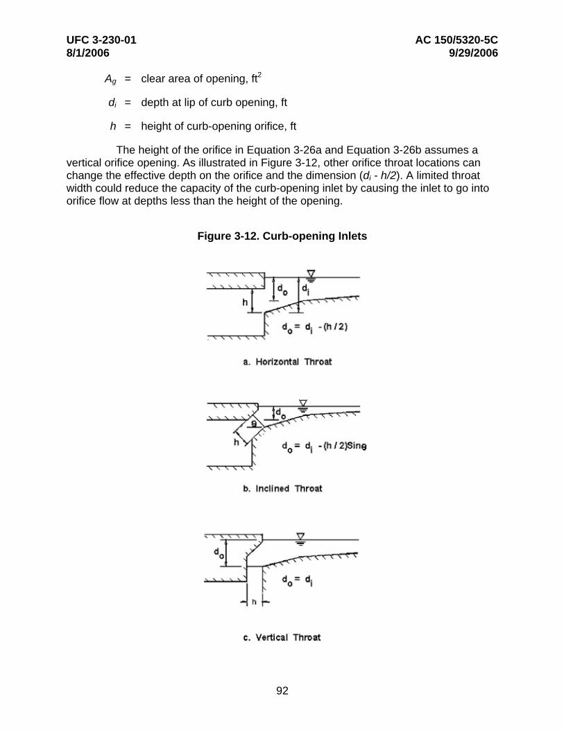
The height of the orifice in Equation 3-26a and Equation 3-26b assumes a vertical orifice opening. As illustrated in Figure 3-12, other orifice throat locations can change the effective depth on the orifice and the dimension (di - h/2). A limited throat width could reduce the capacity of the curb-opening inlet by causing the inlet to go into orifice flow at depths less than the height of the opening.

Figure 3-12. Curb-opening Inlets

92

UFC 3-230-01 AC 150/5320-5C 8/1/2006 9/29/2006

3-5.5.2.9 For curb-opening inlets with other than vertical faces (see Figure 3-12), Equation 3-26a can be used with:

h = orifice throat width, ft

do = effective head on the center of the orifice throat, ft

Chart 10 provides solutions for Equation 3-23 and Equation 3-26 for depressed curb-opening inlets, and Chart 11 provides solutions for Equation 3-25 and Equation 3-26 for curb-opening inlets without depression. Chart 12 is provided for use for curb openings with other than vertical orifice openings. Example 3-10 illustrates the use of Chart 11 and Chart 12.

Example 3-10

Given: Curb-opening inlet in a sump location with:

L = 8.2 ft

h = 0.432 ft

(1) Undepressed curb opening:

Sx = 0.02

T = 8.2 ft

(2) Depressed curb opening:

Sx = 0.02

a = 1

W = 2 ft

T = 8.2 ft

Find: Qi

Solution (1): Undepressed

Step 1. Determine the depth at curb.

d = T Sx = (8.2)(0.02)

d = 0.16 ft

d = 0.16 ft ≤ h = 0.43 ft, therefore weir flow controls

93

UFC 3-230-01 AC 150/5320-5C 8/1/2006 9/29/2006

Step 2. Use Equation 3-25 or Chart 11 to find Qi.

Qi = Cw L d 1.5

Qi = (3.0)(8.2)(0.16)1.5

= 1.6 ft3/s

Solution (2): Depressed

Step 1. Determine the depth at curb, di.

di = d + a

di = Sx T + a

di = (0.02)(8.2) + 1/12

di = 0.25 ft

di = 0.25 ft < h = 0.43 ft, therefore weir flow controls

Step 2. Determine the efficiency of the curb opening.

P = L + 1.8 W

P = 8.2 + (1.8)(2.0)

P = 11.8 ft

1.5Qi = Cw (L + 1.8 W ) d

Qi = (2.3)(11.8)(0.16)1.5

= 1.7 ft3/s

The depressed curb-opening inlet has 10 percent more capacity than an inlet without depression.

3-5.6 Inlet Locations. The location of inlets is determined by geometric controls that require inlets at specific locations, the use and location of flanking inlets in sag vertical curves, and the criterion of spread on the pavement. In order to adequately design the location of the inlets for a given project, specific information is needed:

A layout or plan sheet suitable for outlining drainage areas

Road or runway profiles

Typical cross sections

94

UFC 3-230-01 AC 150/5320-5C 8/1/2006 9/29/2006

Grading cross sections

Superelevation diagrams

Contour maps

3-5.6.1 Geometric Controls. In a number of locations, inlets may be necessary with little regard to the contributing drainage area. These locations should be marked on the plans prior to any computations regarding discharge, water spread, inlet capacity, or flow bypass. These are examples of such locations:

At all low points in the gutter grade

Immediately upstream of median breaks, entrance/exit ramp gores, cross walks, and street intersections, i.e., at any location where water could flow onto the travelway

Immediately up grade of bridges (to prevent pavement drainage from flowing onto bridge decks)

Immediately downstream of bridges (to intercept bridge deck drainage)

Immediately up grade of cross slope reversals

Immediately up grade from pedestrian cross walks

At the end of channels in cut sections

On side streets immediately up grade from intersections

Behind curbs, shoulders, or sidewalks to drain low areas

In addition to these areas, runoff from areas draining towards the pavement should be intercepted by roadside channels or inlets before it reaches the roadway. This applies to drainage from cut slopes, side streets, and other areas alongside the pavement. Curbed pavement sections and pavement drainage inlets are inefficient means for handling extraneous drainage.

3-5.6.2 Inlet Spacing on Continuous Grades. Design spread is the criterion used for locating storm drain inlets between those required by geometric or other controls. The interception capacity of the upstream inlet will define the initial spread. As flow is contributed to the gutter section in the downstream direction, spread increases. The next downstream inlet is located at the point where the spread in the gutter reaches the design spread. Therefore, the spacing of inlets on a continuous grade is a function of the amount of upstream bypass flow, the tributary drainage area, and the gutter geometry.

3-5.6.2.1 For a continuous slope, the designer may establish the uniform design spacing between inlets of a given design if the drainage area consists of pavement only

95

UFC 3-230-01 AC 150/5320-5C 8/1/2006 9/29/2006

or has reasonably uniform runoff characteristics and is rectangular in shape. In this case, the time of concentration is assumed to be the same for all inlets. The following procedure and example illustrate the effects of inlet efficiency on inlet spacing.

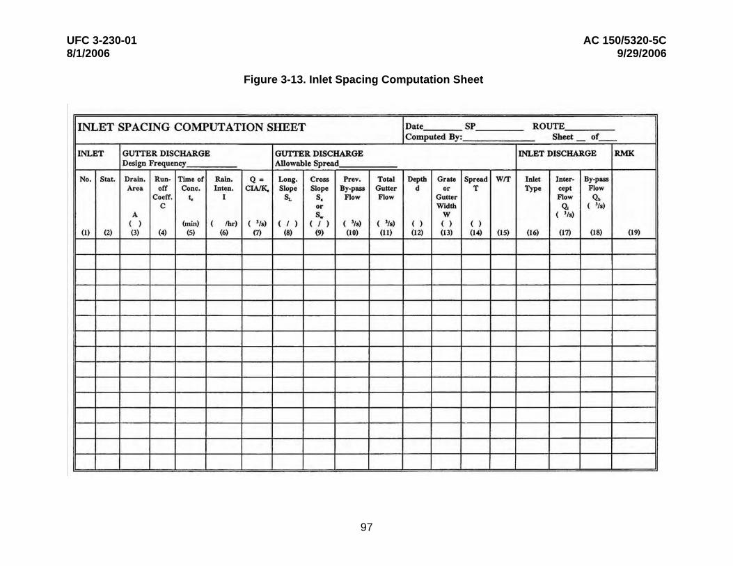
3-5.6.2.2 In order to design the location of inlets on a continuous grade, the computation sheet shown in Figure 3-13 may be used to document the analysis. A step-by-step procedure for the use of Figure 3-13 follows.

Step 1. Complete the blanks at the top of the sheet to identify the job by state project number, route, date, and your initials.

Step 2. Mark on a plan the location of inlets that are necessary even without considering any specific drainage area, such as the locations described in section 3-5.6.1.

Step 3. Start at a high point, at one end of the job if possible, and work towards the low point. Then begin at the next high point and work backwards toward the same low point.

Step 4. To begin the process, select a trial drainage area approximately 300 to 500 ft long below the high point and outline the area on the plan. Include any area that may drain over the curb, onto the roadway. However, where practical, drainage from large areas behind the curb should be intercepted before it reaches the roadway or gutter.

Step 5. Col. 1 Describe the location of the proposed inlet by number (col. 1) and station (col. 2) and record this.

Col. 2 Information in columns 1 and 2. Identify the curb and gutter type in Column 19.

Col. 19 Remarks. A sketch of the cross section should be prepared.

Step 6. Col. 3 Compute the drainage area (acres) outlined in Step 4 and record in Column 3.

Step 7. Col. 4 Determine the runoff coefficient, C, for the drainage area. Select a C value provided in Table 2-1 or determine a weighted C value using Equation 3-2 and record the value in Column 4.

Step 8. Col. 5 Compute the time of concentration, tc, in minutes, for the first inlet and record it in Column 5. The tc is the amount of time it takes for the water to flow from the most hydraulically remote point of the drainage area to the inlet, as discussed in Chapter 2. The minimum tc is 5 minutes.

96

UFC 3-230-01 AC 150/5320-5C 8/1/2006 9/29/2006

Figure 3-13. Inlet Spacing Computation Sheet

97

UFC 3-230-01 AC 150/5320-5C 8/1/2006 9/29/2006

98

UFC 3-230-01 8/1/2006

AC 150/5320-5C 9/29/2006

Step 9. Col. 6 Using the time of concentration, tc, determine the rainfall intensity from the IDF curve for the design frequency. Enter the value in Column 6.

Step10. Col. 7 Calculate the flow in the gutter using Equation 3-1, Q = CIA. The flow is calculated by multiplying Column 3 times Column 4 times Column 6. Enter the flow value in Column 7.

Step 11. Col. 8 From the roadway profile, enter in Column 8 the gutter longitudinal slope, SL, at the inlet, taking into account any superelevation.

Step12. Col. 9 From the cross section, enter the cross slope, Sx, in Column 9 and the grate or gutter width, W, in Column 13.

Step13. Col. 11 For the first inlet in a series, enter the value from Column 7 into Column 11 since there was no previous bypass flow. Additionally, if the inlet is the first in a series, enter 0 into Column 10.

Step14. Col. 14 Determine the spread, T, by using Equations 3-2 and 3-4 or Chart 1 and Chart 2 and enter the value in Column 14. Also, determine the depth at the curb, d, by multiplying the spread by the appropriate cross slope, and enter the value in Column 12. Compare the calculated spread with the allowable spread as determined by the design criteria outlined in section 3.2. Additionally, compare the depth at the curb with the actual curb height in Column 19. If the calculated spread, Column 14, is near the allowable spread and the depth at the curb is less than the actual curb height, continue on to Step 15. Otherwise, expand or decrease the drainage area up to the first inlet to increase or decrease the spread, respectively. The drainage area can be expanded by increasing the length to the inlet, and it can be decreased by decreasing the distance to the inlet. Then, repeat Steps 6 through 14 until you obtain the appropriate values.

Step 15. Col. 15 Calculate W/T and enter the value in Column 15.

Step 16. Col. 16 Select the inlet type and dimensions and enter the values in Column 16.

Step 17. Col. 17 Calculate the flow intercepted by the grate, Qi, and enter the value in Column 17. Use Equations 3-11 and 3-8 or Chart 2 and Chart 4 to define the gutter flow. Use Chart 5 and Equation 3-14 or Chart 6 to define the flow intercepted by the grate. Use Equations 3-17 and 3-18 or Chart 7 and Chart 8 for curb-opening inlets. Finally, use Equation 3-16 to determine the intercepted flow.

99

UFC 3-230-01 8/1/2006

AC 150/5320-5C 9/29/2006

Step 18. Col. 18 Determine the bypass flow, Qb, and enter it into Column 18. The bypass flow is Column 11 minus Column 17.

Step 19. Col. 1-4 Proceed to the next inlet down the grade. To begin the procedure, select a drainage area approximately 300 to 400 ft below the previous inlet for a first trial. Repeat Steps 5 through 7 considering only the area between the inlets.

Step 20. Col. 5 Compute the time of concentration, tc, for the next inlet based upon the area between the consecutive inlets and record this value in Column 5.

Step 21. Col. 6 Determine the rainfall intensity from the IDF curve based on the time of concentration, tc, determined in Step 20 and record the value in Column 6.

Step 22. Col. 7 Determine the flow in the gutter by using Equation 3-1 and record the value in Column 7.

Step 23. Col. 11 Record the value from Column 18 of the previous line into Column 10 of the current line. Determine the total gutter flow by adding Column 7 and Column 10 and record the value in Column 11.

Step 24. Col. 12 Determine the spread and the depth at the curb as outlined in Step 14. Repeat Steps 18 through 24 until the spread and the depth at the curb are within the design criteria.

Step 25. Col. 16 Select the inlet type and record it in Column 16.

Step 26. Col. 17 Determine the intercepted flow in accordance with Step 17.

Step 27. Col. 18 Calculate the bypass flow by subtracting Column 17 from Column 11. This completes the spacing design for the inlet.

Step 28. Repeat Steps 19 through 27 for each subsequent inlet down to the low point. HEC-22 provides an example that illustrates the use of this procedure and Figure 3-13.

For inlet spacing in areas with changing grades, the spacing will vary as the grade changes. If the grade becomes flatter, inlets may be spaced at closer intervals because the spread will exceed the allowable spread. Conversely, for an increase in slope, the inlet spacing will become longer because of increased capacity in the gutter sections. Additionally, individual transportation agencies may limit spacing due to maintenance constraints.

100

UFC 3-230-01 AC 150/5320-5C 8/1/2006 9/29/2006

3-5.6.3 Flanking Inlets. As explained in section 3-5.6.2, inlets should always be located at the low or sag points in the gutter profile. In addition, it is good engineering practice to place flanking inlets on each side of the low point inlet when in a depressed area that has no outlet except through the system. This is illustrated in Figure 3-14. The purpose of the flanking inlets is to act in relief of the inlet at the low point if it should become clogged or if the design spread is exceeded. For a complete explanation of the application of flanking inlets, see section 3-5.5. To summarize, flanking inlets should be used when the runoff entering the sag has only one exit location, i.e., the inlet in the bottom of the sag and the depth of ponding caused by clogging at the low point would cause a hazardous condition. An example would be a sag at an underpass. If the depth of ponding does not become too great and the runoff can exit over the curb, then flanking inlets may not be necessary.

Figure 3-14. Example of Flanking Inlets

Example 3-11

Given: A 500-ft (L) sag vertical curve at an underpass on a 4-lane divided highway with begin and end slopes of -2.5 percent and +2.5 percent respectively. The spread at design Q is not to exceed the shoulder width of 9.8 ft.

Sx = 0.02

Find: The location of the flanking inlets if located to function in relief of the inlet at the low point when the inlet at the low point is clogged.

Solution:

Step 1. Find the rate of vertical curvatures, K.

LK = (Send − Sbeginning )

101

UFC 3-230-01 AC 150/5320-5C 8/1/2006 9/29/2006

500ftK = (2.5% − (− 2.5%))

K = 100 ft

Step 2. Determine the depth at the curb at the design spread.

d = Sx T = (0.02)(9.84)

d = 0.2 ft

Step 3. Determine the depth for the flanker locations.

d = 63 percent of depth over the inlet at the bottom of the sag (see Figure 3-14)

= 0.63 (0.2)

= 0.13 ft

Step 4. For use with Table 3-6:

d = 0.20 - 0.13 = 0.07 ft

X = distance from sag point, (200dK)0.5

= {(200)(0.07)(100)}0.5

= 37.4 ft

The inlet spacing is 37.4 ft from the sag point.

3-5.6.3.1 Flanking inlets can be located so they will function before water spread exceeds the allowable spread at the sump location. The flanking inlets should be located so that they will receive all of the flow when the primary inlet at the bottom of the sag is clogged. They should do this without exceeding the allowable spread at the bottom of the sag. If the flanking inlets are the same dimension as the primary inlet, they will each intercept one-half the design flow when they are located so that the depth of ponding at the flanking inlets is 63 percent of the depth of ponding at the low point. If the flanking inlets are not the same size as the primary inlet, it will be necessary to either develop a new factor or do a trial and error solution using assumed depths with the weir equation to determine the capacity of the flanking inlet at the given depths.

3-5.6.3.2 Table 3-6 shows the spacing required for various depth at curb criteria and vertical curve lengths defined by K = L / (G2 - G1), where L is the length of the vertical curve in feet and G1 and G2 are the approach grades in percent. The AASHTO policy on geometrics specifies maximum K values for various design speeds and a maximum K of 167 considering drainage. The use of Table 3-6 is illustrated in Example 3-11.

102

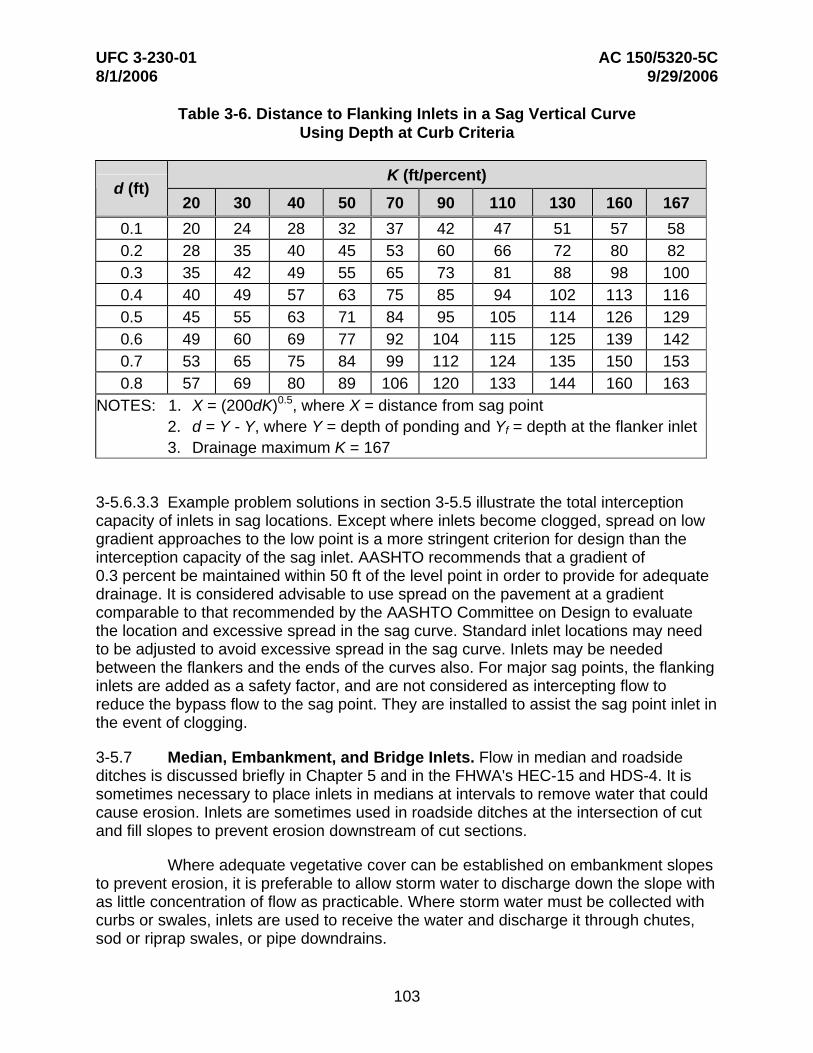
UFC 3-230-01 AC 150/5320-5C 8/1/2006 9/29/2006

Table 3-6. Distance to Flanking Inlets in a Sag Vertical Curve Using Depth at Curb Criteria

d (ft) K (ft/percent)

20 30 40 50 70 90 110 130 160 167 0.1 20 24 28 32 37 42 47 51 57 58 0.2 28 35 40 45 53 60 66 72 80 82 0.3 35 42 49 55 65 73 81 88 98 100 0.4 40 49 57 63 75 85 94 102 113 116 0.5 45 55 63 71 84 95 105 114 126 129 0.6 49 60 69 77 92 104 115 125 139 142 0.7 53 65 75 84 99 112 124 135 150 153 0.8 57 69 80 89 106 120 133 144 160 163

NOTES: 1. X = (200dK)0.5, where X = distance from sag point 2. d = Y - Y, where Y = depth of ponding and Yf = depth at the flanker inlet 3. Drainage maximum K = 167

3-5.6.3.3 Example problem solutions in section 3-5.5 illustrate the total interception capacity of inlets in sag locations. Except where inlets become clogged, spread on low gradient approaches to the low point is a more stringent criterion for design than the interception capacity of the sag inlet. AASHTO recommends that a gradient of 0.3 percent be maintained within 50 ft of the level point in order to provide for adequate drainage. It is considered advisable to use spread on the pavement at a gradient comparable to that recommended by the AASHTO Committee on Design to evaluate the location and excessive spread in the sag curve. Standard inlet locations may need to be adjusted to avoid excessive spread in the sag curve. Inlets may be needed between the flankers and the ends of the curves also. For major sag points, the flanking inlets are added as a safety factor, and are not considered as intercepting flow to reduce the bypass flow to the sag point. They are installed to assist the sag point inlet in the event of clogging.

3-5.7 Median, Embankment, and Bridge Inlets. Flow in median and roadside ditches is discussed briefly in Chapter 5 and in the FHWA's HEC-15 and HDS-4. It is sometimes necessary to place inlets in medians at intervals to remove water that could cause erosion. Inlets are sometimes used in roadside ditches at the intersection of cut and fill slopes to prevent erosion downstream of cut sections.

Where adequate vegetative cover can be established on embankment slopes to prevent erosion, it is preferable to allow storm water to discharge down the slope with as little concentration of flow as practicable. Where storm water must be collected with curbs or swales, inlets are used to receive the water and discharge it through chutes, sod or riprap swales, or pipe downdrains.

103

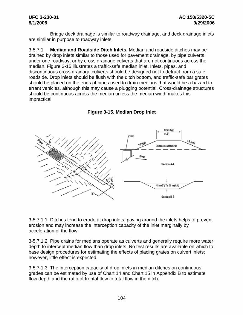
UFC 3-230-01 AC 150/5320-5C 8/1/2006 9/29/2006

Bridge deck drainage is similar to roadway drainage, and deck drainage inlets are similar in purpose to roadway inlets.

3-5.7.1 Median and Roadside Ditch Inlets. Median and roadside ditches may be drained by drop inlets similar to those used for pavement drainage, by pipe culverts under one roadway, or by cross drainage culverts that are not continuous across the median. Figure 3-15 illustrates a traffic-safe median inlet. Inlets, pipes, and discontinuous cross drainage culverts should be designed not to detract from a safe roadside. Drop inlets should be flush with the ditch bottom, and traffic-safe bar grates should be placed on the ends of pipes used to drain medians that would be a hazard to errant vehicles, although this may cause a plugging potential. Cross-drainage structures should be continuous across the median unless the median width makes this impractical.

Figure 3-15. Median Drop Inlet

3-5.7.1.1 Ditches tend to erode at drop inlets; paving around the inlets helps to prevent erosion and may increase the interception capacity of the inlet marginally by acceleration of the flow.

3-5.7.1.2 Pipe drains for medians operate as culverts and generally require more water depth to intercept median flow than drop inlets. No test results are available on which to base design procedures for estimating the effects of placing grates on culvert inlets; however, little effect is expected.

3-5.7.1.3 The interception capacity of drop inlets in median ditches on continuous grades can be estimated by use of Chart 14 and Chart 15 in Appendix B to estimate flow depth and the ratio of frontal flow to total flow in the ditch.

104

UFC 3-230-01 AC 150/5320-5C 8/1/2006 9/29/2006

3-5.7.1.4 Chart 14 is the solution to Manning's equation for channels of various side slopes. Manning's equation for open channels is:

Q = 1.486 AR 0.67SL 0.5 (3-27)

n

where:

Q = discharge rate, ft3/s

n = hydraulic resistance variable

A = cross-sectional area of flow, ft2

R = hydraulic radius = area/wetted perimeter, ft

SL = bed slope, ft/ft

3-5.7.1.5 For the trapezoidal channel cross section shown on Chart 14, Manning's equation becomes:

0.67

Q = 1.486 (B + zd 2 )⎛⎜⎜ B + zd 2 ⎞

⎟⎟ SL 0.5 (3-28)

n ⎝ B + 2d z2 + 1⎠

where:

B = bottom width, ft

z = horizontal distance of the side slope to a rise of 1 ft vertical, ft

Equation 3-28 is a trial and error solution to Chart 14.

3-5.7.1.6 Chart 15 is the ratio of frontal flow to total flow in a trapezoidal channel. This is expressed as:

W oE (B + dz) (3-29)

3-5.7.1.7 Chart 5 and Chart 6 are used to estimate the ratios of frontal and side flow intercepted by the grate-to-total flow.

3-5.7.1.8 Small dikes downstream of drop inlets (Figure 3-15) can be provided to impede bypass flow in an attempt to cause complete interception of the approach flow. The dikes usually need not be more than a few inches high and should have traffic safe slopes. The height of dike required for complete interception on continuous grades or the depth of ponding in sag vertical curves can be computed by use of Chart 9. The effective perimeter of a grate in an open channel with a dike should be taken as

105

UFC 3-230-01 AC 150/5320-5C 8/1/2006 9/29/2006

2(L + W) since one side of the grate is not adjacent to a curb. Use of Chart 9 is illustrated in section 3-5.5.1.2.

3-5.7.1.9 The following examples illustrate the use of Chart 14 and Chart 15 for drop inlets in ditches on continuous grade.

Example 3-12

Given: A median ditch with these characteristics:

B = 3.9 ft

n = 0.03

z = 6

S = 0.02

The flow in the median ditch is to be intercepted by a drop inlet with a 2 ft by 2 ft P-50 parallel bar grate; there is no dike downstream of the inlet.

Q = 9.9 ft3/s

Find: The intercepted and bypassed flows (Qi and Qb)

Solution:

Step 1. Compute the ratio of frontal to total flow in a trapezoidal channel.

Qn = (9.9)(0.03)

Qn = 0.30 ft3/s

From Chart 13:

d = 0.12 B

( )d = B ⎛⎜⎝

d B⎞⎟⎠

= (0.12)(3.9)

= 0.467 ft

Using Equation 3-29 or Chart 15:

106

UFC 3-230-01 AC 150/5320-5C 8/1/2006 9/29/2006

Eo =

=

=

Step 2.

V =

A =

A =

V =

=

W

(B + dz)

2.0 [3.9 + (0.47)( ) 6 ]

0.30

Compute the frontal flow efficiency.

Q

A

(0.47)[(6)(0.47) + 3.9]

3.18 ft2

9.9 3.18

3.11 ft/s

From Chart 5, Rf = 1.0

Step 3. Compute the side flow efficiency.

Since the ditch bottom is wider than the grate and has no cross slope, use the least cross slope available on Chart 6 or use Equation 3-14 to solve for Rs.

Using Equation 3-14 or Chart 6:

1Rs = ⎛ 0.15V 1.8 ⎞⎜⎜1+ 2.3 ⎟⎟⎝ SxL ⎠

1Rs = ⎛ (0.15)( 3.11)1.8 ⎞ ⎜⎜1+ {(0.01)( 2.0)2.3 }⎟⎟ ⎝ ⎠

= 0.04

Step 4. Compute the total efficiency.

E = EoRf + Rs(1 - Eo)

E = (0.30)(1.0) + (0.04)(1 - 0.30)

107

UFC 3-230-01 AC 150/5320-5C 8/1/2006 9/29/2006

= 0.33

Step 5. Compute the interception and bypass flow.

Qi = E Q

Qi = (0.33)(9.9)

Qi = 3.27 ft3/s

Qb = Q - Qi

Qb = (9.9) - (3.27)

Qb = 6.63 ft3/s

In the above example, a P-1-7/8 inlet would intercept about 33 percent of the flow in a 3.9-ft bottom ditch on a continuous grade.

For grate widths equal to the bottom width of the ditch, use Chart 6 by substituting ditch side slopes for values of Sx, as illustrated in Example 3-13.

Example 3-13

Given: A median ditch with these characteristics:

Q = 9.9 ft3/s

W = 2 ft

z = 6

S = 0.03 ft/ft

B = 2 ft

n = 0.03

Sx = 0.17 ft/ft

The flow in the median ditch is to be intercepted by a drop inlet with a 2 ft by 2 ft P-1-7/8 parallel bar grate. There is no dike downstream of the inlet.

Find: The intercepted and bypassed flows (Qi and Qb).

Solution:

Step 1. Compute the ratio of frontal to total flow in a trapezoidal channel.

Qn = (9.9)(0.03)

108

UFC 3-230-01 AC 150/5320-5C 8/1/2006 9/29/2006

Qn = 0.30 ft3/s

From Chart 14:

d = 0.25 B

d = (0.25)(2.0)

= 0.50 ft

Using Equation 3-29 or Chart 15:

WEo = (B + dz)

2.0 = [2.0 + (0.5)( ) 6 ]

= 0.40

Step 2. Compute the frontal flow efficiency.

QV = A

A = (0.5)[(6)(0.5) + 2.0]

A = 2.5 ft2

9.9V = 2.5

= 4.0 ft/s

From Chart 5, Rf = 1.0

Step 3. Compute the side flow efficiency.

Using Equation 3-14 or Chart 6:

1Rs =⎛ 0.15V 1.8 ⎞⎜⎜1+ ⎟⎟⎝ SxL

2.3 ⎠

109

UFC 3-230-01 AC 150/5320-5C 8/1/2006 9/29/2006

1Rs = ⎛ (0.15)( 4.0)1.8 ⎞⎜⎜ 2.3 }⎟⎟⎝ 1+ {(0.17)( 2.0) ⎠

= 0.32

Step 4. Compute the total efficiency.

E = EoRf + Rs(1 - Eo)

E = (0.40)(1.0) + (0.32)(1 - 0.40)

= 0.59

Step 5. Compute the interception and bypass flow.

Qi = E Q

Qi = (0.59)(9.9)

Qi = 5.83 ft3/s

Qb = Q - Qi

Qb = (9.9) - (5.83)

Qb = 4.07 ft3/s

The height of dike downstream of a drop inlet required for total interception is illustrated by Example 3-14.

Example 3-14

Given: Data from Example 3-13.

Find: The required height of a berm to be located downstream of the grate inlet to cause total interception of the ditch flow.

Solution:

P = 2(L + W)

P = 2(2.0 + 2.0)

= 8.0 ft

110

UFC 3-230-01 AC 150/5320-5C 8/1/2006 9/29/2006

Using Equation 3-21 or Chart 9:

0.67

d = ⎢⎣

⎡(C

Q

w

i

P )⎥⎦⎤

⎡ (9.9) ⎤0.67

d = ⎢⎣{(3.0)( 8.0)}⎥⎦

d = 0.55 ft

A dike will need to have a minimum height of 0.55 ft for total interception. Due to the initial velocity of the water that may provide adequate momentum to carry the flow over the dike, an additional 0.5 ft may be added to the height of the dike to ensure complete interception of the flow.

3-5.7.2 Embankment Inlets. Drainage inlets are often needed to collect runoff from pavements in order to prevent erosion of fill slopes or to intercept water upgrade or downgrade of bridges. Inlets used at these locations differ from other pavement drainage inlets in three respects. First, the economies that can be achieved by system design are often not possible because a series of inlets is not used; second, total or near total interception is sometimes necessary in order to limit the bypass flow from running onto a bridge deck; and third, a closed storm drainage system is often not available to dispose of the intercepted flow, and the means for disposal must be provided at each inlet. Intercepted flow is usually discharged into open chutes or pipe downdrains that terminate at the toe of the fill slope.

3-5.7.2.1 Example problem solutions in other sections of this UFC illustrate by inference the difficulty in providing for near total interception on grade. Grate inlets intercept little more than the flow conveyed by the gutter width occupied by the grate. Combination curb-opening and grate inlets can be designed to intercept total flow if the length of curb opening upstream of the grate is sufficient to reduce spread in the gutter to the width of the grate used. Depressing the curb opening would significantly reduce the length of inlet required. Perhaps the most practical inlets or procedure for use where near total interception is necessary are sweeper inlets, increase in grate width, and slotted inlets of sufficient length to intercept 85 to 100 percent of the gutter flow. Design charts and procedures in section 3-5.4 are applicable to the design of inlets on embankments. Figure 3-16 illustrates a combination inlet and downdrain.

3-5.7.2.2 Downdrains or chutes used to convey intercepted flow from inlets to the toe of the fill slope may be open or closed chutes. Pipe downdrains are preferable because the flow is confined and cannot cause erosion along the sides. Pipes can be covered to reduce or eliminate interference with maintenance operations on the fill slopes. Open chutes are often damaged by erosion from water splashing over the sides of the chute due to oscillation in the flow and from spill over the sides at bends in the chute. Erosion at the ends of downdrains or chutes can be a problem if not anticipated. The end of the device may be placed low enough to prevent damage by undercutting due to erosion.

111

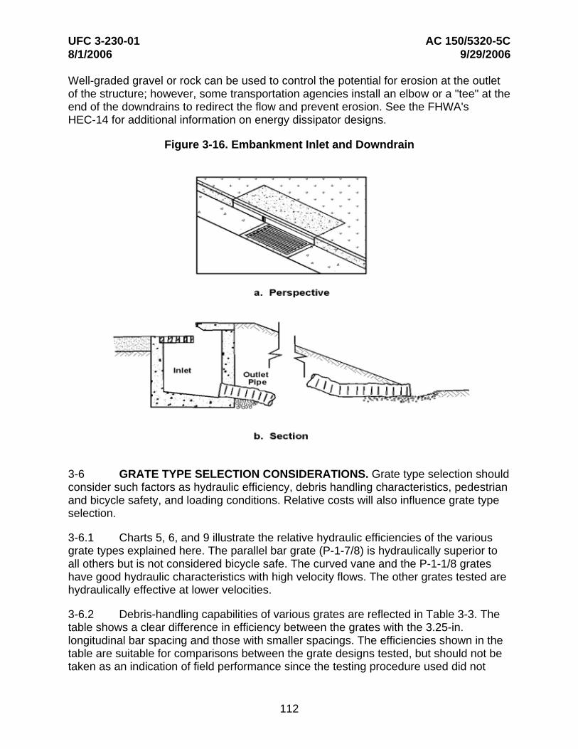
UFC 3-230-01 AC 150/5320-5C 8/1/2006 9/29/2006

Well-graded gravel or rock can be used to control the potential for erosion at the outlet of the structure; however, some transportation agencies install an elbow or a "tee" at the end of the downdrains to redirect the flow and prevent erosion. See the FHWA's HEC-14 for additional information on energy dissipator designs.

Figure 3-16. Embankment Inlet and Downdrain

3-6 GRATE TYPE SELECTION CONSIDERATIONS. Grate type selection should consider such factors as hydraulic efficiency, debris handling characteristics, pedestrian and bicycle safety, and loading conditions. Relative costs will also influence grate type selection.

3-6.1 Charts 5, 6, and 9 illustrate the relative hydraulic efficiencies of the various grate types explained here. The parallel bar grate (P-1-7/8) is hydraulically superior to all others but is not considered bicycle safe. The curved vane and the P-1-1/8 grates have good hydraulic characteristics with high velocity flows. The other grates tested are hydraulically effective at lower velocities.

3-6.2 Debris-handling capabilities of various grates are reflected in Table 3-3. The table shows a clear difference in efficiency between the grates with the 3.25-in. longitudinal bar spacing and those with smaller spacings. The efficiencies shown in the table are suitable for comparisons between the grate designs tested, but should not be taken as an indication of field performance since the testing procedure used did not

112

UFC 3-230-01 AC 150/5320-5C 8/1/2006 9/29/2006

simulate actual field conditions. Some local transportation agencies have developed factors for use of debris-handling characteristics with specific inlet configurations.

3-6.3 Table 3-7 ranks grate styles according to relative bicycle and pedestrian safety. The bicycle safety ratings were based on a subjective test program performed by the FHWA; however, all the grates are considered bicycle and pedestrian safe except the P-1-7/8. In recent years with the introduction of very narrow racing bicycle tires, some concern has been expressed about the P-1-1/8 grate. Exercise caution when using it in bicycle areas.

3-6.4 Grate loading conditions must also be considered when determining an appropriate grate type. Grates in traffic areas must be able to withstand traffic loads; conversely, grates draining yard areas usually do not need to be as rigid.

Table 3-7. Grate Ranking with Respect to Bicycle and Pedestrian Safety

Rank Grate Style 1 P-1-7/8 x 4 2 Reticuline 3 P-1-1/8 4 45° - 3-1/4 Tilt Bar 5 45° - 2-1/4 Tilt Bar 6 Curved Vane 7 30° - 3-1/4 Tilt Bar

113