UCRL-ID-120428

Instructions for Calibrating Gamma Detectors using the Canberra - Nuclear Data Genie Gamma Spectroscopy System

James L. Brunk Health and Ecological Assessment Division

September 1995

Work performed under the auspices of the U.S. Department of Energy by Lawrence Livermore National Laboratory under contract W-7405-Eng-48.

STER

DISCLAIMER

This report was prepared a s an account of work sponsored by an agency of the United States Government. Neither t h e United States Government nor any agency thereof, nor any of their employees, make any warranty, express or implied, or assumes any legal liability or responsibility for the accuracy, completeness, or usefulness of any information, apparatus, product, or process disclosed, or represents that its use would not infringe privately owned rights. Reference herein t o any specific commercial product, process, or service by trade name, trademark, manufacturer, or otherwise does not necessarily constitute or imply its endorsement, recommendation, or favoring by the United States Government or any agency thereof. The views and opinions of authors expressed herein do not necessarily s ta te or reflect those of the United States Government or any agency thereof.

DISCLAIMER

Portions of this document may be illegible in electronic image products. Images are produced from the best available original document.

Table of Contents

1 Note ............................................................................................................................................... Computer Conventions ................................................................................................ 1

Introduction and Background .................................................................................................. 2

System Architecture 5

Calibration Steps 7 Initial Steps 7

Background 8

The Energy and FWHM Calibration ........................................................................... 8 The Efficiency Calibration 8

Comparison of the Results from the Rest of the Standard Set ............................. 9 Record Keeping 9

Notes on Quality Control .......................................................................................................... 9 ................................................................................................................................... 11 References

Appendix A --Required Files for the Standardization Procedure ............................. A-12 Appendix B -- Calibration Check List and Commands ................................................. €3-15 Appendix C -- Detector Installation and Counter Information Sheet ....................... c-18 Appendix D -- Supplemental Command Procedures and Programs ........................ 1t22 Appendix E -- Results an Initial Calibration ................................................................... E-32 Appendix F -- Results of an Update Calibration ............................................................ F-35 Appendix G -- Data Handling Codes and Databases ...................................................... G-39

.......................................................................................................................................... 1

Calibration Principles ..................................................................................................... 3

Preparation for Calibration ..................................................................................................... *.5

Abstract

.......................................................................................................

Standards 5 .......................................................................................................................... ......................................................................................................................... .......................................................................................................................

Standards 7 .............................................................................................................. ..........................................................................................................

.............................................................................................

...............................................................................................................

ii

Note

Computer Conventions

Descriptions of actions performed on various computers are interspersed throughout this report. Bold print denotes the names of programs and other commands. CALIB /INIT is an example of this usage. All commands to the various programs end with an implied carriage return, labeled on some keyboards as enter. Both the VAX/VMS and IBM PC operating systems are case insensitive with respect to program names and operating system commands. However, when the codes and programs are requesting information, the computer stores the data requested just as it receives it and thus these data are case sensitive. Items enclosed in angle brackets (e >) are user supplied data that are variable in nature and may changes with each occurrence. An example of this construction is CALIBIINIT <detector name>. Information pertaining to a particular gamma spectrum is stored together in one place in a basic entity referred to as a configuration (Canberra, 1990). This configuration information is media independent; it can exist as a disk file, in an archive or stored in a semiconductor ADC memory area. The configuration files that contain the specific calibration information for a particular detector system and geometry combination reside on the VAX'S system disk. Since this information is important at later times, thesystem is programmed to mark them read only automatically in the VMS log in command file. This gives some protection against accidental erasure. Be aware, however, that the system manager's account contains all privileges including the one to override write protection. Thus, the system manager must guard against inadvertently erasing these files during a global file purge. The Digital Equipment VMS computer system stores the name and location information about isotope property library files, spectral configurations, files describing the radiological properties of the standards and other needed fie in Digital Command Language (DCL) logical names and system symbols. The data manipulation programs create and use these logical names and symbols as default program parameters. This provides a convenient method to shorten the commands required to calculate a desired result when using a string of operations.

Abstract

A straight forward protocol provides a way to guide the calibration of a gamma detector for a particular geometry and material. Several programs have used the

1

Low Level Gamma Counting Facility of the Health and Ecological Assessment Division of the Lawrence Livermore National Laboratory to count a variety of large environmental samples contained in several unique geometries. The equipment and calibration requirements needed to analyze these types of samples are explained. This document describes the calibration protocol that has been developed and describes how it is used to calibrate the detectors.

Introduction and Background

The mission of the Low Level Gamma Counting Facility of the Health and Ecological Assessment (HEA) Division of the Lawrence Livermore National Laboratory (LLNL) is to provide the expertise and equipment to perform nondestructive assays of gamma emitting radionuclides contained in a variety of sample matrices. The HEA Division and its predecessors have had facilities to determine the concentrations of gamma emitting radionuclides found in the environment since the 1960's (Allen, 1994). These facilities have evolved into the Low Level Gamma Counting Facility. Recently, due to changes in the central LLNL computing environment and the impending obsolesce of the data collection systems, changes to the counting system architecture and analysis scheme had to be made. After investigation of several systems, the GENIE@ system manufactured by Canberra - Nuclear Datal was selected. This system allows for the collection of spectral data from several detectors while simultaneously doing data reduction calculations on a Digital Equipment Corporation* (DEC) VAStation* running DEC's VMS@ operating system. This new system has the advantage of a great decrease in the amount of time required to calibrate a geometry when compared with the previous method (Brunk, 1989). With the prior method, several standards were counted and a time consuming manual procedure took many days of effort to produce the required calibration parameters. With this new system, a standard is counted and three programs supplied by the manufacturer calculate the calibration parameters in a manner of minutes. This empirical approach eliminates the need to calculate many of the parameters that the previous method required. The trade off for this ease of calibration is that if the experimenter's samples do not substantially match the standard in elemental composition and geometry, the measured activities will deviate from the correct ones by an uncharacterized amount. This effect is compensated for by carefully selecting the materials that make up the calibration standards taking care to match the physical properties of the samples as closely as possible.

I Canberra Industries Inc., Nuclear Data Systems Division, 150 Spring Lake Dr., Itasca, IL 60143- 2096.

2 Digital Equipment Corporation, Maynard, Massachusetts.

2

Calibra fion Principles

Calibration is the process of identifying and documenting the characteristic parameters of a detector and signal processing system. The effort required to calibrate a system varies with the demands of the calculation scheme. The previous code, GAMANAL, a code written by members of the LLNL Nuclear Chemistry Division, calculated the answers using a complete mathematical description of the various system variables that involved a time consuming calibration procedure (Gunnink, 1972; Brunk, 1989)- Our current calculation scheme relies on having the calibration standards as close as possible in geometry and material composition as the samples of interest. With the current system, there are two basic calibrations required for sufficient detector characterization. They are the energy versus channel number relationship that includes a full width at half peak maximum (FWHM) characterization and an efficiency versus energy calibration. Two characterizations that are not performed are the count pile-up correction and the coincidence summing error correction. Pulse pile up occurs when two gammas arrive at the detector within the width of the amplifier's output pulse. The low emission rates of the typical environmental level samples (much less than the 1000 s-1 specified in ANSI, 1991) allow US to neglect the error contributions from pulse pile-up. Coincidence summing is radionuclide, geometry and detector dependent. When counting samples that emit coincident gamma rays at window to sample distances less than 10 cm, a graph of summing correction versus ktector to sample distance is constructed. Factors read from this graph are used to mrrect the activities. The energy versus channel number calibration describes the relationship between the channel number and the gamma energy. The calibration software provided with the GENIE system calculates offset, slope and quadratic factors so that the following equation describes the relationship (Canberra, 1989).

energy = offset + (slope - channel) + (quadratic - Energy is the calculated energy at the specified channel. The units are

determined by the* entry in the file that describes the standard's characteristics (See Appendix A).

channel analyzer (MCA) channel number in which the centroid 'of the peak resides.

Channel is the multi

Offset is the number of channels the spectrum is shifted. Slope and quadratic are the calculated fit coefficients.

The FWHM describes the peak shape. This shape varies with peak energy and is a function of the physical construction of the detector and the bias voltage. The system uses the following equation to calculate the FWHM (Canberra, 1989).

3

FWHM = onset + slope , / G i

FWHM is the difference in energy between the two points on the peak curve that OCCUPY the half the maximum peak height. The units are the same as those used for reporting the peak energy.

Energy is the value of the energy at the centroid of the peak. Offset and slope are the calculated coefficients.

The detector efficiency coefficient describes the relationship between number of gamma rays emitted at a particular energy that deposit all of its energy in the detector and number of the counts detected.

Where: E is the gamma photo peak efficiency in counts/g I? is the integrated peak area in counts Q is the calibration source mass or volume quantity in grams, ml, etc. R is the calibration source emission rate at a particular reference time in

y/second/(mass or volume quantity) TI is the elapsed time during which the detector system can process

gamma rays measured in seconds (referred to as live time) TI is the real time in seconds which is the elapsed live count time plus

the time that the system is incapable of processing a second gamma ray (referred to as dead time)

Ts is the source decay time (the acquisition start time subtracted from the calibration source zero time)

h is the decay constant in seconds” (also equal to In 2 divided by the nuclide half life, tl,J

The program calculates an efficiency for each of the described gamma rays in the standard and fits a curve to the set of energy - efficiency pairs. This efficiency ~ ~ r v e may be described in one of two ways. The software vendor refers to these as empirical, which is calculated via cubic splines, and non-empirical, which is calculated using a least square fit routine. The spline method assumes that with N calibration energies, N-1 third order polynomials exist such that the first and second derivatives are continuous at the each of the energies. By definition, the resulting curve passes through each of the energy points. This method is very local in nature causing a maximum extrapolation of 10 keV at the ends of the curve. The least squares fit method does not have this extrapolation restriction. equation is a global analytical function of the form:

The

4

In@) = "t + 4 a x +a4 a x 2 +a, a x 3 +a, ex4 +a, * x 5

Where: E is the calculated efficiency in countsly x is ln(al / E) E is the peak energy at which the efficiency is calculated in keV a1 is (El- E,)/2 El is the energy of the least energetic gamma ray in the standard E2 is the energy of the more energetic gamma ray in the standard a2 through a, are the fit parameters

The calibration software starts with three degrees of freedom and calculates the fit parameters. The program uses a reduced chi squared test to inspect the curve. If the test is close to 1.0, the curve fits the data set well. If the test is below 0.8, the set is over determined and fewer fit parameters are needed. If the test is over 2.0, the set is underdetermined and more parameters are needed. The software iterates this process until a convergence occurs, a chi square of greater than 2.0 with a fifth order polynomial occurs, a chi square of less than 0.8 with a second order polynomial occurs or if one fit gives a chi squared of less than 0.8 and the next order fit gives a test of over 2.0. In the last case, the fit with less than 0.8 is used (Canberra, 1989). System Architecture

The facility currently has 20 gamma detectors in use. The types used are lithium drifted germanium (Ge(Li)) and high purity germanium (HPGe) detectors. Each detector has its own high voltage power supply and spectroscopy amplifier. The output from each amplifier connects to one of the input ports of an eight port mixer router module. The output of the routers connects to a fast analog to digital converter (ADC) that is connected to a communication control interface that transmits the digital data over thin Ethernet to the VAX computer. All of the instrumentation bins are bonded to a common ground point via a heavy wire bus to prevent ground loops. This bus is connected to the building ground at only one point so all the instrumentation shares the same ground potential. The spectroscopy package runs on a time share basis and processes the spectral information for real time display. At the conclusion of the count, the computer stores the data on the local disk for subsequent processing. As part of the data security program, an automatic tape backup occurs each night for both the system and data disks.

Preparation for Calibration Standards

Since the result of a calculation is very dependent on the sample geometry and composition, the calibration scheme requires at least one standard for each sample

5

geometry (Canberra, 1990). A set of standards prepared in such a way as to be very close to identical in composition containing a particular material in a particular geometry are used. Currently there are calibrations for four materials; a water phantom made of epoxy resin, ammonium molybdophosphate microcrystals (AMP), shredded macaroon coconut, flaked dehydrated potato granules and coral soil. These materials cover a range of densities (0.5 to 2.0 g cm-3) and elemental makeup of environmental sample materials. (Kehl, 1995) A steel can and a plastic vial, act as the primary counting containers. The construction of the standard materials requires a great deal of experience and care. (ANSI, 1991, NCRP, 1985.) Bulk standard ingredients were prepared to our specifications by contractors not associated with this laboratory. This permitted the specification of the isotopes, the activity levels and degree of homogeneity for the standard materials. National Institute of Standards and Technology (NIST) traceability of the standard materials was an important requirement. For the initial calibration effort, the contracting laboratory was Isotope Products Laboratory.3 This vendor provided approximately 50 kg of each standard matrix in bulk form. Final calibration standards were constructed by canning aliquants of the bulk material using the same procedures used to can experimental samples. The term calibration implies traceability to a universally recognized value. The standard formulation contract between LLNL and the external contractor specified that all final standard materials would be traceable to NIST. The contracting vendor complied with this requirement by participating in the Radioactivity Measurements Assurance Program conducted by NIST in cooperation with the US. Council of Energy Awareness (USCEA). In the program, NIST provided blind samples for assaying by the participating labs, with the results sent back to NIST. NIST reported back the difference between the NIST certified value and the lab's value. In addition to this program, the vendor also sends finished products to NIST for product verification and calibration. (IPL, 1993.) The procurement Specifications required a certificate of calibration for each batch of standard material. These certificates provided statements of traceability and complete descriptions of the physical and nuclear properties of the materials. The calibration codes require files containing the radiological information about the standards. These files, called certificate files, contain the sample mass, zero time, sample identification and radiological characteris tics of each isotope present in the standard source. Since individual standards differ slightly in construction, each must have its own certificate file created for it using the software vendor's Certificate File Editor (CFE) (Canberra, 1990). See appendix A for a discussion of certificate files. A library describing the isotopes in the standard must exist. The Nuclide Library Editor program (NLE), supplied by the software vendor does this task (Canberra, 1990). See appendix A for an example of a library output listing.

Isotope Products, Corporate and Sales Offices, 3017 N. San Fernando Blvd., Burbank, CA 91504. 3

Calibration Steps

Refer to appendix B for a synopsis of the calibration protocol. Initial Steps

The detector is set up as described in appendix C. The first stage in the calibration procedure requires that the amplifier be brought into rough energy calibration. This is done as described above during the detector set up by counting a standard containing ' T o and inspecting the spectrum for the correct channel versus energy relationship. The amplifier gain controls are adjusted until the centroid of the 1332 keV peak is located in channel 2665. This indicates that the channel - energy relationship of the spectra is about 0.5 keV per channel. In the current scheme, a full spectrum uses 4096 channels which equates to approximately 2 MeV for the whole spectrum. The zero adjustment on the analog to digital converter (ADC) acts to position the spectra at the low energy end. Due to the current electronic setup with up to eight detectors sharing the ADC input through a mixer - router module, the adjustment to the zero control occurs once at the ADC's initial installation. This common control affects the position of the spectra from all the detectors on a particular mixer/router combination. (ASTM, 1993, ASTM, 1987)

Standards

When calibrating a detector system for a particular geometry and sample material, an appropriate set of like standards is counted. One standard of the set is selected as a particular detector's calibrating standard. The activities from this particular standard are used as the benchmarks to compare the activities calculated from rest of the set. This protocol requires that each member of the set be counted for approximately the same live time. The factors determining the count time are the activities of the isotopes present, taking into account the branching ratio of the least abundant gamma ray of interest, and the time since the reference date of the standard. The standards are counted until the least abundant peak described in the calibration certificate file has a peak error below one percent. Several pieces of identifying information are necessary to set up the various command procedures needed to calibrate a geometry. These other pieces of data such as the sample weight, sample name, count time, zero time, detector name and geometry are extracted from the configuration file. The VMS command procedure make-info.com extracts this information about the count by inspecting its configuration and extracting the needed data items. (see appendix D) This procedure creates a text file containing a list of the items of interest. The data is checked for validity paying close attention to the detector name, geometry, sample name and the sample quantity. Any corrections are made with the pardscreen program. The data extracted from this file is used as input data to create the command files with programs like inforec.com. (see appendix D)

7

Backaou nd

Samples with amounts of activity approaching limits of detection often require long count times. The side effect of long count times is that background radiation shows up in the spectra. The radionuclides contained in the building and cave construction materials as well as those naturally occurring in the soil and surroundings contribute to this environmental background. This effect is accounted for by subtracting the time weighted activity of a long (approximately 6000 minute) background count from the activity of a sample. The background count consists of a spectrum taken with nothing in the sample holder. This approach differs from other methods involving counting an empty container or a container filled with water. The channel position - peak energy relationship of the spectrum is inspected with the vendor supplied peak program. The centroids from a few peaks from the commonly occurring background isotopes, such as 4% and 228U daughters, are compared with the expected channel values. Any needed adjustment in the expected channel location versus energy relationship is made using the calibration program. The command used is CALIB /INIT /cer=cstandard certificate7 <configuration>. This configuration becomes the file containing the background subtraction information. He copies it to the system disk and renames it with a name in the form: xx-background.cnf where xx is the first two characters of the detector name. The move command accomplishes this. The Energy and FWHM Calibration

The initial energy and full width at half maximum calibration occurs by issuing a CALIBRATE /INITIAL <detector name> command at the VAX keyboard. The program asks for the positions of the peaks flagged in the certificate file as those to be used in an initial calibration. As a check, a peak search occurs next by issuing the PEAK /LIST=$PRINTER command. The peak energy values obtained are compared with the correct energies for those peaks. See Appendix E for an example. The Efficiency Calibration

After any adjustment of the peak energies, an update calibration is next performed. The do,calibrate.com DCL command procedure is used to calculate efficiencies with a polynonial fit. If a spline fit is desired, the do-calibrate-noemp.com DCL command procedure is used to complete the update calibration. (See appendix D> An example of the calibration report is found at appendix F. The peak positions are checked by calculating again with the PEAK /LIST=$PRINTER command. If the peaks have not shifted, the efficiency plot is displayed with the EFF /PLOT /LOG command. The curve should be a smooth bell shaped curve skewed to the low energy side. The final step is to run the identification routine, N I D /LIST=$PRINTER. If the calculated activities are within the acceptable error, u~ually plus or minus five percent of the certificate value, the move command is used to copy the standard configuration file to the system disk with a name in the form of: XX-F-TYPEcnf. The XX is the first two letters of the detector name, the F is a designator indicating the amount of sample material in the in the geometry (for

8

example, F for full, H for half full), and TYPE is a description of the standard matrix (for example, water, soil, potato or coconut). Comparison of the Results from the Rest of the Standard Set

The remainder of the standard set spectra are calculated using the newly calculated efficiency parameters. The use of the new-calc.com DCL command procedure with the standard library and the normal background file makes this task easier. (see appendix D) Tabulate the results and compare the activities sorted with respect to standard number with the amounts listed on the standard certificate. Files containing the calculated activities are produced and have names in the form XX-######A.txt. The XX is the user code, the ###### is the spectrum ID number and the A is an alphanumeric indicating the recalculation position. A FORTRAN code located in appendix G is used to change the format of the activity data produced by the NID program to one that can be used with a data base program. The structure listing of the data base is also found in appendix G. If the values are in satisfactory agreement with the certificate values (usually plus or minus five percent), the calibration is complete. See appendix G for examples of the printouts from the various steps. Record Keeping

The term calibration also implies traceability. The records and printouts generated in the calibration process are retained in permanent storage. The calibration is not considered complete until a hard copy of the data is stored in binders and the calibration files are stored in the electronic archives.

Notes on Quality Control

Quality Control (QC) is the process undertaken to provide confidence in a particular result. The Quality Control program in use at the gamma counting facility has two major parts. The first part deals with the accuracy, precision and freedom from contamination of the whole sample process. The second deals with the consistency of the procedures and equipment used for the determination. Each part is the responsibility of separate group of individuals. A prudently designed experimental program will take steps to implement the first part, measuring how well the facility analyzes the sample set. Blind duplicates, blanks and external standards are added to the sample sets sent for analysis. This blind method provides a level of checking that thoroughly test the facility's capabilities. The standards contain well-known amounts of certain isotopes chosen for their properties which test channel - energy shifts, efficiency changes and detector contamination of the counting systems. Usually several isotopes are included in the standard to give a range of gamma ray energies. The activities reflect those of the routine samples. The results of these standard determinations show how accurate the measurements are. The duplicate samples allow the

9

experimenter to compare the precision of several measurements. The blanks show if contamination is present. The other part of the QC program is performed at the counting facility. Special attention is paid to the calibration process making sure that a counting system is not put into service until it performs consistently within the desired precision and accuracy levels. After a system is put into service, weekly measurements designed to detect deviations from these levels are done as part of the routine counting program. The purpose of this portion is to monitor the performance of the counting systems and make any needed adjustments to the software parameters or electronics as to produce the correct answer for particular standards. Background counts are performed once a week to keep the systems under surveillance to make sure that the detectors and caves are not contaminated by leaky samples. Also as part of their part of the Quality Control program, changes made during software development and maintenance are recorded to keep records of the algorithms in use and noting changes in coding or logic. (Canberra, 1989) Between these two QC efforts, the probability of careless errors in the analysis process becomes less likely. To enhance the confidence level further, world wide intercomparison standards are analyzed. An external organization picks a material with the appropriate level of activity to use in the study. Interested laboratories receive aliquants for analysis. The laboratories analyze the sample and report the activity levels to the study's authors who then tabulate and distribute the results to the participants. Comparison of the data demonstrates the competence of a facility with respect to the other participants.

10

References Allen, Michael J., Private communication (1994).

American National Standards Institute and the Institute of Electrical and Electronic Engineers, I E E E Standard Test Procedures for Germanium Gamma-Ray Detectors, ANSI/IEEE 325-1986 (August 13,1986).

American National Standards Ins ti tu te, A merica n Na t iona I S f a nda rd Calibra tion and Use of Germanium Spectrometers for the Measurement of Gamma-Ray Emission Rates of Radionuclides, N42.141991 (July 2, 1991).

American Society for Testing and Materials, Standard Practices for the Measurement of Radioactiuity, D3648-78 (January 27, 1978; Re approval, October 1987).

American Society for Testing and Materials, Standard Methods for Detector Calibration and Analysis of Radionuclides, EM-93 (April 15, 1993).

Brunk, James L., Diode Calibration Manual, Lawrence Livermore National Laboratory, Livermore, CA, M-262 (1989).

Canberra Industries, Ge(Li) Detector Test Procedure and Troubleshooting Guide, Informal Document (July 1, 1976).

Canberra Nuclear Products Group, Spectroscopy Applicaf ions AZgorithms and Software Verification and Validation Manual, 07-0386 (December, 1989).

Canberra Nuclear Products Group, V A X I V M S Spectroscopy Applications User's and Display Manuals, Vol. 1, 07-0196 (November, 1990).

Gunnink, R., J. B. Niday, Computerized Quantitaf ive Analysis by Gamma-ray Spectroscopy, UCRL-51061, Vol. 1-3 (March 1,1972).

Isotope Products Laboratory, Catalog, (1993).

Kehl, Steven R., private communications (1995).

National Council on Radiation Protection and Measurements, A Handbook of Radioactivity Measurements Procedures, NCRP Report No. 58 (February 1, 1985).

US NIM Committee, Standard NZM Instrumentation System, DOE /ER-O457T, (May 1990). [Formerly TID 20893 (Rev) and NIM/GPIB].

Appendix A --Required Files for the Standardization Procedure

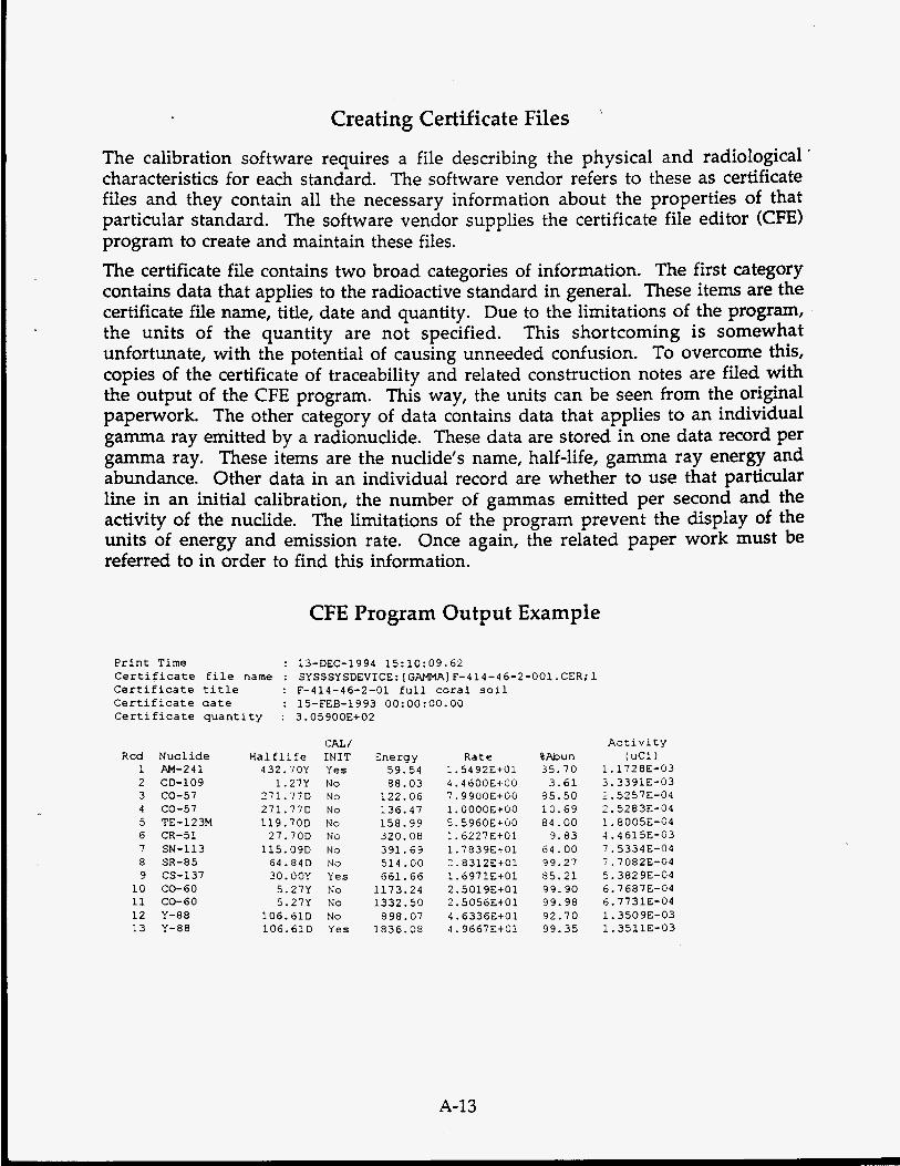
Creating Certificate Files

The calibration software requires a file describing the physical and radiological ’ characteristics for each standard. The software vendor refers to these as certificate files and they contain all the necessary information about the properties of that particular standard. The software vendor supplies the certificate file editor (CFE) program to create and maintain these files. The certificate file contains two broad categories of information. The first category contains data that applies to the radioactive standard in general. These items are the certificate file name, title, date and quantity. Due to the limitations of the program, the units of the quantity are not specified. This shortcoming is somewhat unfortunate, with the potential of causing unneeded confusion. To overcome this, copies of the certificate of traceability and related construction notes are filed with the output of the CFE program. This way, the units can be seen from the original paperwork. The other category of data contains data that applies to an individual gamma ray emitted by a radionuclide. These data are stored in one data record per gamma ray. These items are the nuclide’s name, half-life, gamma ray energy and abundance. Other data in an individual record are whether to use that particular line in an initial calibration, the number of gammas emitted per second and the activity of the nuclide. The limitations of the program prevent the display of the units of energy and emission rate. Once again, the related paper work must be referred to in order to find this information.

CFE Program Output Example

P r i n t Time : 13-DEC-1994 15:10:09.62 C e r t i f i c a t e f i l e name : SYSSSYSDEVICE: [GAMMA] F-414-46-2-001.CER; 1 C e r t i f i c a t e t i t l e : F-414-46-2-01 f u l l cora l s o i l

C e r t i f i c a t e q u a n t i t y : 3.05900E+02 C e r t i f i c a t e d a t e : 15-FEB-1993 OO:OO:OO.OO

R c d N u c l i d e 1 AM-241 2 CD-109 3 CO-57 4 CO-57 5 TE-123M 6 CR-51 7 SN-113 8 SR-85 9 CS-137

10 CO-60 11 CO-60 1 2 Y-80 13 Y-88

H a l f l i f e 432.70Y

1.27Y 271.77D 271.77D 119.70D

27.70D 115.09D

64.84D 30. OOY

5.27Y 5.27Y

106.61D 106.61D

CAL/ INIT Yes N o No No No No No N o Yes N o No N o Yes

Energy 59.54 88 .03

122 .06 136.47 158 .99 320.08 391.69 514.00 661.66

1113.24 1332.50

898 .07 1836.08

R a t e 1.5492EtOl 4 .4600Et00 7 .99006+00 1.0000E+00

I. 6227E+01 1 . 7 8 3 9E+01 2.8312E+01

2.5019E+01 2.5056E+01 4.6336€+01 4.9667E+01

5.5960EtirO

1.6971E+01

%Abun 35 .70 3.61

85 .50 10 .69 84.00

9 . 8 3 64.00 99 .27 85 .21 9 9 - 9 0 99.98 92.70 99 .35

A c t i v i t y [ uCi 1

1.1728E-03 3.3391E-03 2.5257E-04 2.5283E-04 1. & O O 5 E - O 4 4 . 4 61 5E-03 7.5334E-04 7.7082E-04 5.38296-04 6.1687E-04 6.7731E-04 1.3509E-03 1.3511E-03

A-13

-

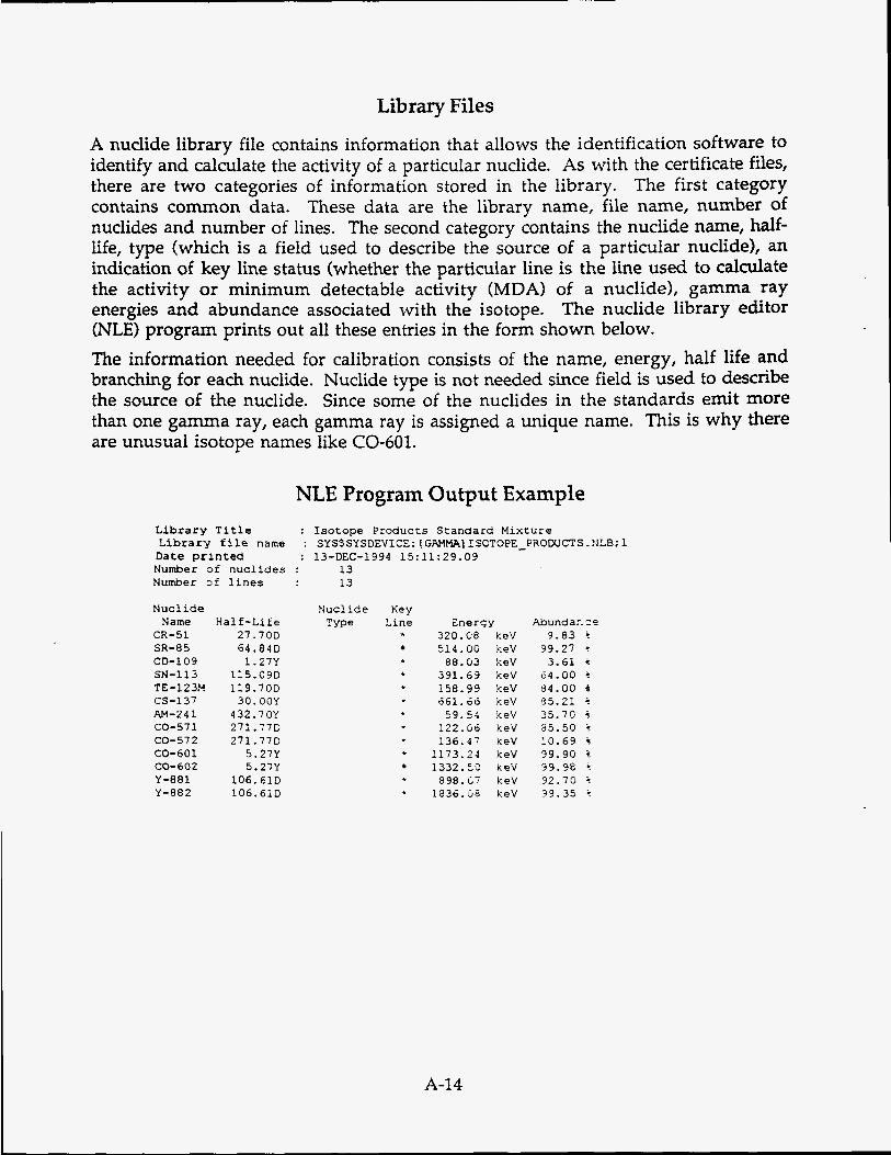
Library Files

A nuclide library file contains information that allows the identification software to identify and calculate the activity of a particular nuclide. As with the certificate files, there are two categories of information stored in the library. The first category contains common data. These data are the library name, file name, number of nuclides and number of lines. The second category contains the nuclide name, half- life, type (which is a field used to describe the source of a particular nuclide), an indication of key line status (whether the particular line is the line used to calculate the activity or minimum detectable activity (MDA) of a nuclide), gamma ray energies and abundance associated with the isotope. The nuclide library editor (NLE) program prints out all these entries in the form shown below. The information needed for calibration consists of the name, energy, half life and branching for each nuclide. Nuclide type is not needed since field is used to describe the source of the nuclide. Since some of the nuclides in the standards emit more than one gamma ray, each gamma ray is assigned a unique name. This is why there are unusual isotope names like CO-601.

NLE Program Output Example Library T i t l e : Isotope Products Standard Mixture L ibrary f i l e name : SYSSSYSDEVICE: [GAMMA) ISOTOPE-PRODUCTS.NLB; 1 Date printed : 13-DEC-1994 15:11:29.09 Number 3f n u c l i d e s : 13 Number of l i n e s : 13

N u c l i d e Nucl ide Key Name Half -Li fe Type L i n e Cnerqy

CR-51 SR-85 CD-109 SN-113 TE-123H CS-137 AM-241 CO-571 CO-572 CO-601 CO-602 Y-881 Y-882

21.70D 64.84D 1.27Y

115.09D 119.70D 30. OOY

432.70Y 271.771) 271.771)

5.27Y 5.27Y

106.61D 106.61G

..

+ 320.08 k e V 514.00 keV 88.G3 k e V

+ 391.63 k e V * 158.55 k e V * 661.66 keV

59.54 keV + 122.06 k e V + 136.47 k e V + 1173.21 keV

1332.50 k e V * 998.C7 k e V

1836.06 k e V

A-1 4

Abundar. .=e 9.83 r

39.27 + 3.61 6

64.00 b 84.00 8 95.21 i 35.70 5 85.50 i 10.69 4 39.90 b 39.98 + 92.7G i 39.35 +

Appendix B - Calibration Check List and Commands

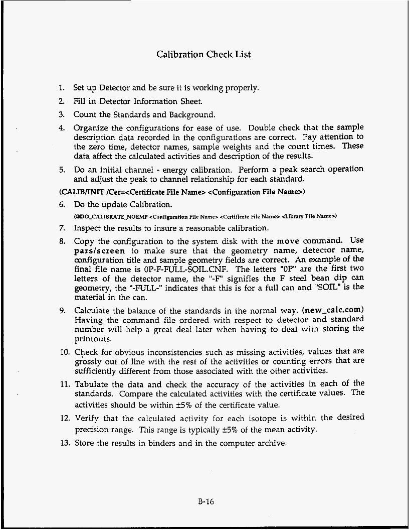
Calibration Check List

Set up Detector and be sure it is working properly. Fill in Detector Information Sheet. Count the Standards and Background. Organize the configurations for ease of use. Double check that the sample description data recorded in the configurations are correct. Pay attention to the zero time, detector names, sample weights and the count times. These data affect the calculated activities and description of the results. Do an initial channel - energy calibration. Perform a peak search operation and adjust the peak to channel relationship for each standard.

1. 2. 3. 4.

5.

(CALIBlINIT /Cer=<Certificate File Name> <Configuration File Name>) 6.

7. 8.

9.

IO.

11.

12.

13.

Do the update Calibration.

Inspect the results to insure a reasonable calibration. Copy the configuration to the system disk with the move command. Use p a r d s c r e e n to make sure that the geometry name, detector name, configuration title and sample geometry fields are correct. An example of the final file name is OP-F-FULL-SOIL.CNF. The letters "OP" are the first two letters of the detector name, the 'I-F" signifies the F steel bean dip Can geometry, the "-FULL-" indicates that this is for a full can and "SOIL" is the material in the can. Calculate the balance of the standards in the normal way. (new-calc.com) Having the command file ordered with respect to detector and standard number will help a great deal later when having to deal with storing the printouts. Check for obvious inconsistencies such as missing activities, values that are glbssly out of line with the rest of the activities or counting errors that are sufficiently different from those associated with the other activities. Tabulate the data and check the accuracy of the activities in each of the standards. Compare the calculated activities with the certificate values. The activities should be within +5% of the certificate value. Verify that the calculated activity for each isotope is within the desired precision range. This range is typically +5% of the mean activity. Store the results in binders and in the computer archive.

(@DO-CALIBRATE-NOEMP <Configuration File Name> <Certificate File Name> <Library File Name>)

B-16

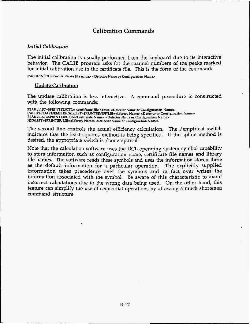
Calibration Commands

Initial Calibration

The initial calibration is usually performed from the keyboard due to its interactive behavior. The CALIB program asks for the channel numbers of the peaks marked for initial calibration use in the certificate file. This is the form of the command: CALIB IINITICER=ccertificate file name> <Detector Name or Configuration Name>

UDdate Ca libration

The update calibration is less interactive. A command procedure is constructed with the following commands: PEAK kIST=SPRINTERICER= certificate file name> <Detector Name or Configuration Name> CALIBNPDATUEMPIRICAULIST~PRINTERIEFF/LIB=<Libra~ Name> <Detector or Configuration Name> PEAK lLIST=SPRINTERICER=cCertificate Name> <Detector Name or Configuration Name> NIDkIST=SPRINTEWLIB=<Libra~ Name> <Detector Name or Configuration Name>

The second line controls the actual efficiency calculation. The /empirical switch indicates that the least squares method is being specified. If the spline method is desired, the appropriate switch is /nonempirical Note that the calculation software uses the DCL operating system symbol capability to store information such as configuration name, certificate file names and library file names. The software reads these symbols and uses the information stored there as the default information for a particular operation. The explicitly supplied information takes precedence over the symbols and in fact over writes the information associated with the symbol. Be aware of this characteristic to avoid incorrect calculations due to the wrong data being used. On the other hand, this feature can simplify the use of sequential operations by allowing a much shortened command structure.

B-17

Appendix C -- Detector Installation and Counter Information Sheet

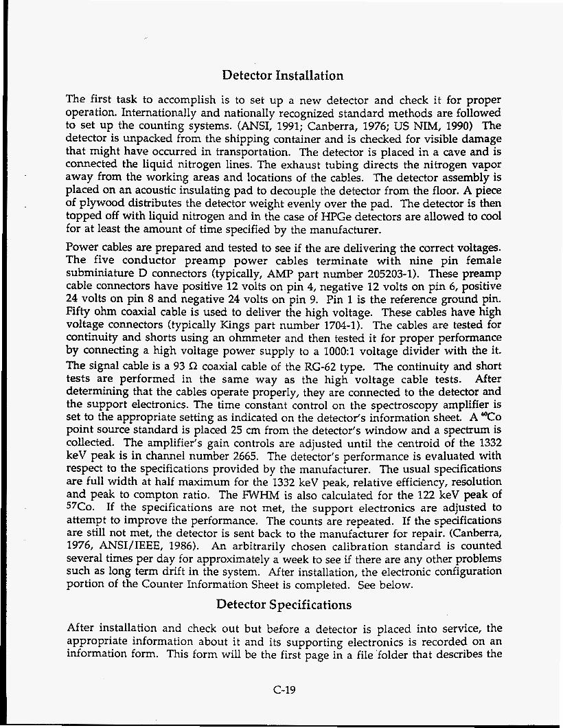
Detector Installation

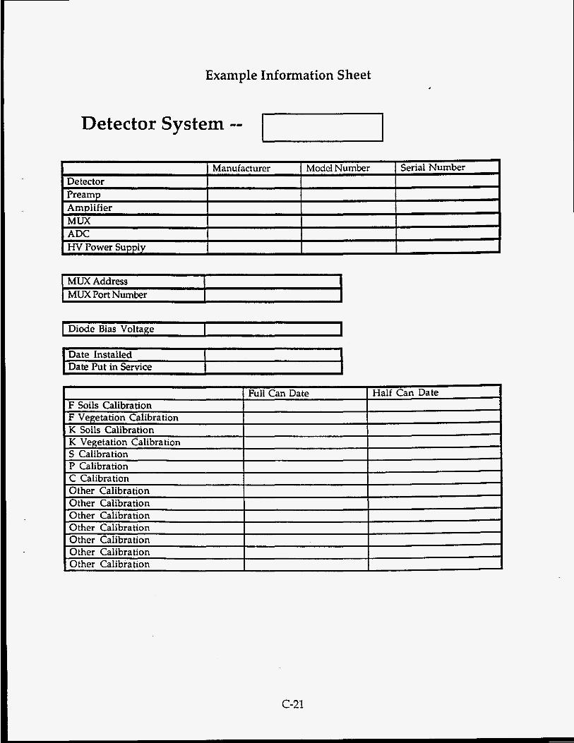
The first task to accomplish is to set up a new detector and check it for proper operation. Internationally and nationally recognized standard methods are followed to set up the counting systems. (ANSI, 1991; Canberra, 1976; US NIM, 1990) The detector is unpacked from the shipping container and is checked for visible damage that might have occurred in transportation. The detector is placed in a cave and is connected the liquid nitrogen lines. The exhaust tubing directs the nitrogen vapor away from the working areas and locations of the cables. The detector assembly is placed on an acoustic insulating pad to decouple the detector from the floor. A piece of plywood distributes the detector weight evenly over the pad. The detector is then topped off with liquid nitrogen and in the case of HPGe detectors are allowed to COO^ for at least the amount of time specified by the manufacturer. Power cables are prepared and tested to see if the are delivering the correct voltages. The five conductor preamp power cables terminate with nine pin female subminiature D connectors (typically, AMP part number 205203-1). These preamp cable connectors have positive 12 volts on pin 4, negative 12 volts on pin 6, positive 24 volts on pin 8 and negative 24 volts on pin 9. Pin 1 is the reference ground pin. Fifty ohm coaxial cable is used to deliver the high voltage. These cables have high voltage connectors (typically Kings part number 1704-1). The cables are tested for continuity and shorts using an ohmmeter and then tested it for proper performance by connecting a high voltage power supply to a 1000:1 voltage divider with the it. The signal cable is a 93 R coaxial cable of the RG-62 type. The continuity and short tests are performed in the same way as the high voltage cable tests. After determining that the cables operate properly, they are connected to the detector and the support electronics. The time constant control on the spectroscopy amplifier is set to the appropriate setting as indicated on the detector's information sheet. A @'co point source standard is placed 25 cm from the detector's window and a spectrum is collected. The amplifier's gain controls are adjusted until the centroid of the 1332 keV peak is in channel number 2665. The detector's performance is evaluated with respect to the specifications provided by the manufacturer. The usual specifications are full width at half maximum for the 1332 keV peak, relative efficiency, resolution and peak to compton ratio. The FWHM is also calculated for the 122 keV peak of 57C0. If the specifications are not met, the support electronics are adjusted to attempt to improve the performance. The counts are repeated. If the specifications are still not met, the detector is sent back to the manufacturer for repair. (Canberra, 1976, ANSI/IEEE, 1986). An arbitrarily chosen calibration standard is counted several times per day for approximately a week to see if there are any other problems such as long term drift in the system. After installation, the electronic configuration portion of the Counter Information Sheet is completed. See below.

Detector Specifications

After installation and check out but before a detector is placed into service, the appropriate information about it and its supporting electronics is recorded on an information form. This form will be the first page in a file folder that describes the

c-19

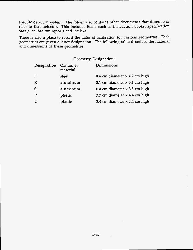
specific detector system. The folder also contains other documents that describe Or refer to that detector. This includes items such as instruction books, specification sheets, calibration reports and the like. There is also a place to record the dates of calibration for various geometries. Each geometries are given a letter designation. The following table describes the materid and dimensions of these geometries.

Geometry Designations Designation Container Dimensions

F steel 8.4 cm diameter x 4.2 cm high K aluminum 8.1 cm diameter x 5.1 cm high S aluminum 6.0 cm diameter x 3.8 cm high P plastic 3.7 cm diameter x 4.4 cm high C plastic 2.4 cm diameter x 1.4 an high

material

e-20

Example Information Sheet

Detector System =-

I MUXAddress I I I MUXPortNumber I I

Diode Bias Voltage I I Date Installed I Date Put in Service

Other Calibration Other Calibration Other Calibration Other Calibration Other Calibration

c-21

Appendix D -- Supplemental Command Procedures and Programs

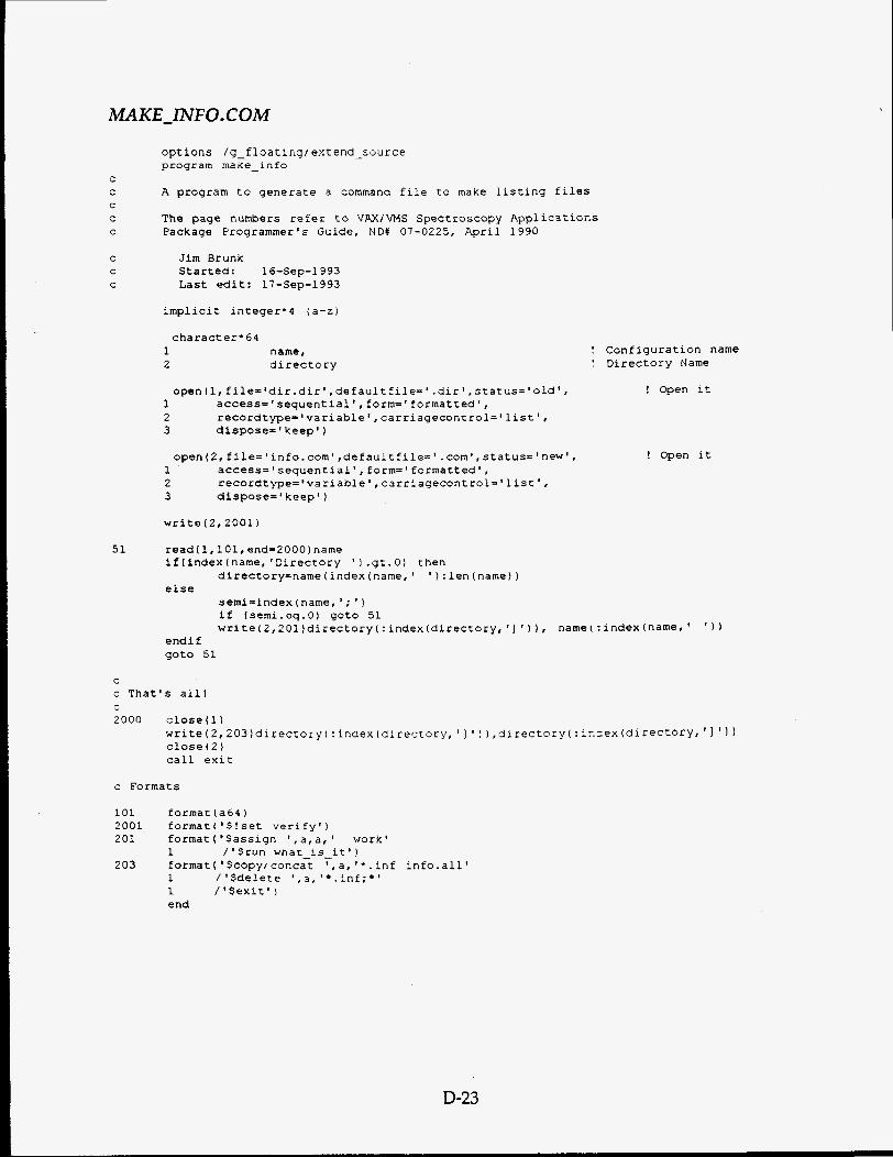
MAKE-RVFO. COM

C C

C

51

options /g-floating/extend-source program make-info

A program to generate a command file to make listing files

The paqe numbers refer to VAX/VMS Spectroscopy App1icatior.s Package Programmer's Guide, ND# 07-0225, April 1990

Jim Brunk Started: 16-Sep-1993 Last edit: 17-Sep-1993

implicit integer'4 (a-z)

character'64 1 name, 2 directory

open(l,file='dir.dir',defaultfile='.dir',status='old', 1 access='sequential',form='formatted', 2 recordtype='variable',carriaqecontrol='list', 3 dispose='keep')

open(2,file='info.com',defaultfileI'.com',status='new', 1 access='sequential',form='formatted', 2 recordtype='variable',carriagecontrol='list', 3 dispose='keep')

! Configuration name ! Directory Name

! Open it

! Open it

read( 1,101, end=2000) name if(index(name,'Directory '1.gt.O) then

else directory=name(index(name,' '):len(name))

semi=index(name,';') if (semi.eq.0) goto 51 write(Z,2Ol)directory(:index(directoryl'] ' I ) , name(:index(name,' ' 1 )

endi f goto 51

C

c That's all1

2000 close ( 1 ) write(2,203)directory(:index(directory,'1 ' ) ) , d i r e c t o r y ( : - - = e x ( d i r e c t o r y , ' ] ' ) ) close ( 2 1 call exit

C

c Formats

101 format (a64 ) 2001 format ( '$!set verify' ) 201 format ( '$assign I , a, a, ' work'

2 0 3 format('$copy/concat ',a, '*.inf info.al1' 1 /'$run what-is-it')

1 / ' $delete I , a, ' . inf ; ' 1 /'$exit' ) end

D-23

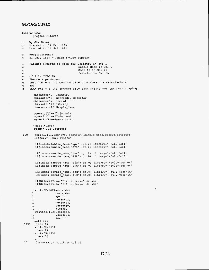
NOREC.FOR

Snotruncate program Inforec

C 5:

C

By Jim Brunk Started : 14 Dec 1993 Last edit: 21 Jul 1994

Modifications: 21 July 1994 - Added T-tube support InfoRec expects to find the Geometry in col 1

Sample Name in Col 2 Spec ID in C o l 18 Detector in Col 25

of file 1NFO.IN ... The code produces: 1NFO.COM - a DCL command file that does the calculations and PEAK.PK2 - a DCL command file that prints out the peak shaping.

character'l Geometry character'2 usercode, detector characteP6 specid character'l3 library characterfl5 Sample-Name

open ( 1, file= Info. in I ) open(Z,file='Info.com') open(3,file='peak.pk2')

write (* , 201) read(*,202)usercode

100 read(l,lOl,end=9999)geomerry, sample-name, Specrd,detector library='-full-Potato'

i f ( index ( s amp1 e-name , ' spr ' ) . g t . 0 1 ib ra ry= ' - f ul1 -Soi 1 ' if(index(samp1e-name, 'SPR') .gt.Ol library='-full-Soil'

if ( index (sample-name, 'ssr' ) .gt. 0) library= -full-Soil ' if(index(samp1e-name,'SSR').gt.O) library='-full-Soil'

if(index(sample-name.'pfa').gt.O) library='-full-Coconut' if(index(sample-name,tPFA').gt.O) library=#-full-Coconut'

i f (index ( sample-name, ' pfd ' ) . g t . 0) 1 i bra ry= - full -Coconut ' if(index(samp1e-name,'PFD').qt.Ol library='-full-Coconut'

if(Geornetry.eq.'T') library='-3q-ampt if(Geometry.eq.'t') library='-3q-amp'

write(2,102)usercode, 1 usercode, 1 specid, 1 detector, 1 detector, 1 geometry, 1 library write ( 3,103 1 usercode,

1 usercode, 1 specid got0 100

3999 close (1 I write (2,199) close ( 2 ) writ e ( 3,19 9 ) close ( 3 ) stop format (al, a15, t18,a6, t25,a21 131

D-24

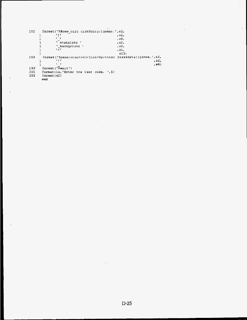
102 format('$@new-calc diskSdata:[gamma.',aZ, & I I 3 ,a2. * , a6, 1 ' etakalpha I ,a2, 1 ' - background ' ,a i l r L 1 - 1 , al,

1

1 I 1 -

a131 103 format('$peak/start=40/list=Sprinter disk$data:[garnrna

1 I 1 ' 1 9 9 forrnat('Sexit*) 201 format(lx,'Enter the User code. ' , $ I 202 format(a2)

end

I ' 1

D-25

',a2, ,a2. ,a6)

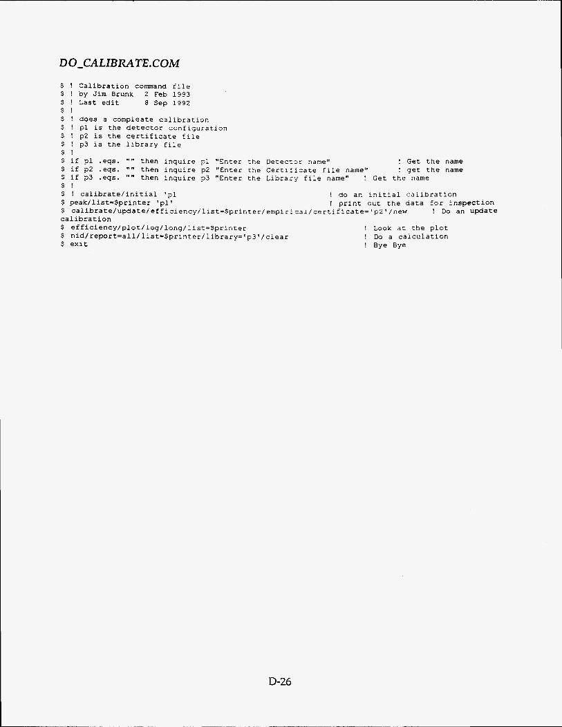
D 0-CALIBRATE.COM

$ ! Calibration command file $ ! by Jim Brunk 2 Feb 1993 $ ! Last edit 8 Sep 1992 $ ! $ ! does a compleate calibration $ ! pl is the detector configuration $ ! p2 is the certificate file $ ! p3 is the library file $ ! $ if p l .eqs. "" then inquire pl "Enter the Deteczsr name" ! Get the name $ if p2 .eqs. "" then inquire p2 "Enter the Certificate file name" ! get the name $ if p3 .eqs. "" then inquire p3 "Enter the Librazy file name" ! Get the name $ ! $ ! calibrate/initial 'pl ! do an initial calibration $ peak/list=$printer ' p l ' ! print out the data for inspection $ calibrate/update/efficiencyjlist=$printer/empir~=al/certificate='~2'/ne~ ! Do an update calibration $ efficiency/plot/log/longjlist=$printer ! LOOK at the plot $ n i d / r e p o r t = a l l / l i s t = S p r i n t e r / l i b r a r y = i p 3 i / c l e a r ! Do a calculation $ exit ! Bye Bye

D-26

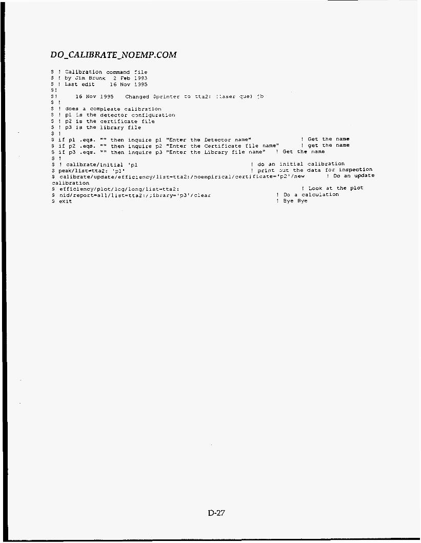
D 0-CALIBRATE-NOEMP. COM

$ ! Calibration command file $ ! by Jim 6runk 2 Feb 1993 $ ! Last edit 16 Nov 1 9 9 5 $ ! $ ! 16 Nov 1995 Changed Sprinter tc tta2: (laser que) jb S ! $ ! does a compleate calibration S ! pl is the detector c3nfiquration S ! p2 is the certificate file $ ! p3 is the library file $ ! s if pl .eqs. '"' then inquire pl "Enter the Detector name" $ if p2 .eqs. '"' then inquire p2 "Enter zhe Certificate file name" $ if p3 .eqs. "" then inquire p3 "Enter the Library file name" ! Get the name $ ! S ! calibrate/initial 'pl ! do an initial calibration $ peak/list=tta2: 'pl' ! print ut the data for inspection S calibrate/update/efficiency/list=ttaZ:f~oempirical/certificate='?~'/new ! Do an update calibration $ efficiency/plot/loq/long/list=tta2: ! L o o k at the plot S nid/report=all/list=tta2:/library='p3'/clear S exit ! Eye Bye

! Get the name ! get the name

! Do a calculation

D-27

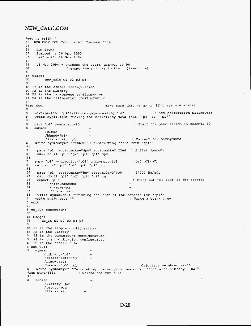
NEW-CALC.COM

$set noverify ! S ! NEW-CALC.COM Calcxlation Commana file $ ! S ! Jim Brunk $ ! Started : 16 Apr 1993 $ ! Last edit: 16 Nov 1994 $ ! $ ! 16 Nov 1994 - changed the s t a r t zhannel to 90 $ ! Changed the printer to tta: (laser que) S ! S ! Usage: $ ! new-calc pl p2 p3 p4 $ ! $ ! P1 is the sample configuration $! PZ is the Library $ ! P3 is the background configuration $ ! P4 is the calibration configuraticn $ ! $set noon ! make sure that we go on if there are errors $ ! S move/partial 'p4'/efficiency/processing ' p l ' $ write syssoutput "Moving the efficiency data from "p4' to "pl" ' $ ! $ pars 'pl' peaKstart=90 ! Start the peak search i n channel 90 $ enback -

/clear - /bkgnd='p3' - / list=tta2: ' pl' ! Correct for background

! Add calibration parameters

$ write sysSoutput "ENBACK is subtracting "p3' from "pl"' $ ! $! pars 'pl' activunits="dpm" activmult=2.22e6 ! 2.22e6 dpm/uCi $ ! call do-it ' p l ' 'pZ' 'p3' lp4' dpm $ ! $ pars 'pl' activunits="pCi" activmult=le6 ! le6 pCi/uCi $ call do-it 'pl' '?Z' 'p3' 'p4' pci $ 2 $! pars 'pl' activunits="Bq" activrr.ult=37000 ! 37000 Bq/uCi S ! call do-it 'pl' 'p2' ' p 3 ' 'p4' bq $ ! report 'pl' ! Print out the rest af the reports $ ! / nid=unknouns - $ ! / header=bq - $ ! /list=tta2: $ ! write sysSoutpuc "Printing the rest of the reports for "pl"' S write sysSoutput "" ! Write a blank l-ne S exit S ! $ do-it: subroutine $ ! S ! Usage: S ! do-it pl p2 p3 p4 p5 S ! S ! P1 is the sample sDnfiquration $ ! P2 is the Library $ ! P3 is the background configuraticr. $! P4 is the calibracion confiqurati-:r: $ ! P5 is the header file $!set veri ! $ wtmean -

- - / 1 ibra ry= ' p2 '

/ report = a ct iv 1 t y /list=tta2: - /header=' p5 ' ' p l ' ! Calcuiate weighted means

$ write sysSoutput "Calculating the weighted means for " p l ' wirn Library "P2"' $run punchfile ! writes the txt file S ! $ minact -

/library= 'p2 ' - /report=mda - /list=tta2: -

D-28

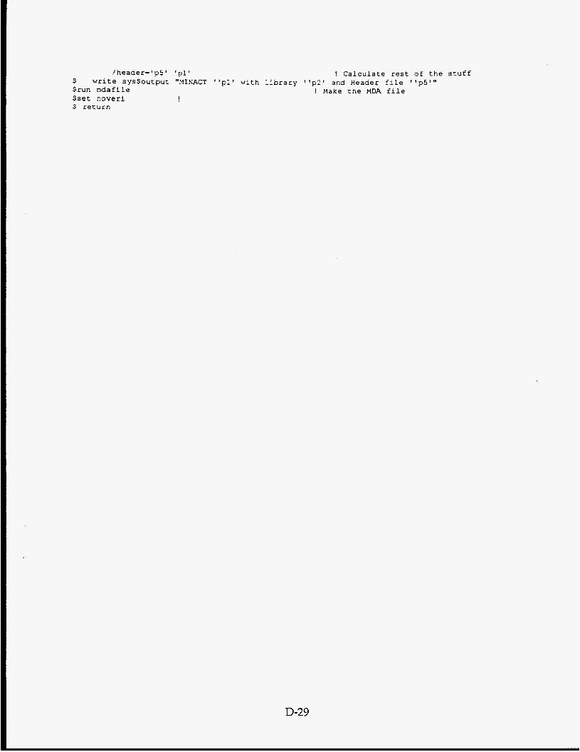
/ h e a a e r = ' p 5 ' ' p i i ! C a l c u l a t e r e s t of t h e s t u f f $ w r i t e S y s S o u t p u t "MINACT " p l ' w i t h L i b r a r y ' l p 2 ' and Header f i l e "p5"' $run r n d a f i l e ! Make t h e MDA f i l e

$ r e t u r n $set noveri !

D-29

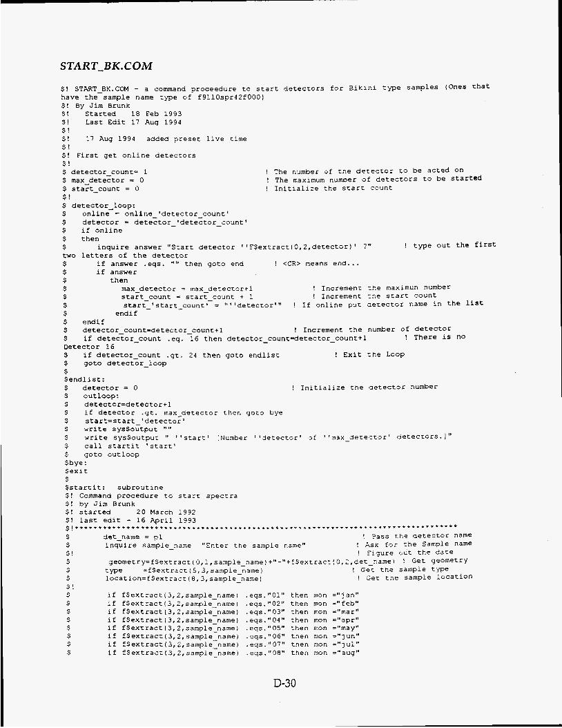
START-BK. COM

s if fSextract s i f f Sext ract $ if fSextract s if fSext ract s if fSext ract s if fSextract s if fSextract

! The number of the aetector to be acted on ! The maximum nilmber of detectors to be started ! Initialize the start count

$! START-BK.COM - a command proceedure to start detectors for Bikini type samples have the sample name type of f9110spr42f000) $! By Jim Brunk $! Started 18 Peb 1993 $ ! Last Edit 17 Aug 1994 $ ! S ! 17 Aug 1994 added preset live time $ ! $! First get online detectors $ ! $ detector-count= 1 $ max-detector = 0 $ start-count = 0 $ ! $ detector-loop: $ online = online-'detector-count' $ detector = detector-'detector-count $ if online $ then $ inquire answer "Start detector "F$extract(O,Z,detector)' ?" two letters of the detector $ if answer .eqs. '"' then goto end $ if answer $ then $ $ s start_'atart-count' = ""detector'" ! If online put aetector name in the list s endif $ endif $ detector-count=detector-count+l ! Increment the number of detector $ if detector-count .eq. 16 then detector-count=detector-count+l ! There is no Detector 16 $ if detector-count .gt. 24 then goto endlist ! Exit the Loop S goto detector-loop $ $ end1 is t : $ detector = 0 ! Initialize the aetector number

S detector=detector+l S if detector .gt. max-detector then goto bye $ start=start-'detector' $ write sysSoutput ""

$ write sys$outpur 11 "start' [Number *',detector' <jf "m~-detezc.>r' detectors. I " $ call startit 'start' $ goto outloop $bye : $exit $ $startit: subroutine $! Command procedure to start spectra $! by Jim Brunk $! started 20 March 1992 $! last edit - 16 April 1993 $ det-name = p l ! pass tne detector name $ inquire sample-name "Enter the sample name" ! ,z.sK fr,r the Sample name S ! ! Fiqure Gut the date s geOmetry=f$eXtract (0,1, sample-name) +"-"tf$extract (0, ;,det-name) ! Get geometry s type =fSextract (5,3,sarnple_name) ! Gec the sample type .$ location=fSextract(8,3,sample-name1 ! set the sample location S ! s

(Ones that

! <CR> means end...

max-detector = max-detectortl ! Increment :he maximun number start-count = start-count t 1 ! Increment 7P.e start count

$ out loop:

$ ~ * * + * + * + * * * + * + * + + + + + * * + * * + + + * + + + * + ~ * * + * + + + * + * ~ * + * * ~ * + + * ~ * * * * + * * . ~ * . + * * * + * + + + + + + + + + *

i f f $ ex t r a c t ( 3 , 2 , s amp 1 e ~ n a me 1 . e qs . '' 0 1 " then mo n = " j an " - 3,2,sample_name) .eqs."02" then mon ="feb" 3,2,sample_name) .eqs."03" then mon ="mar" 3,2,sample-name) .eqs."04" then mon ="apr" 3,2,sample_name) .eqs."05" then rnon ="may" 3,2, sample-name ) . eqs . " 06" then nion =" j un" 3,2,sample_name) .eqs."07" then rnon ="jul" 3,2,sample-narne) .eqs."08" then rnon ="aug"

D-30

! type out the first

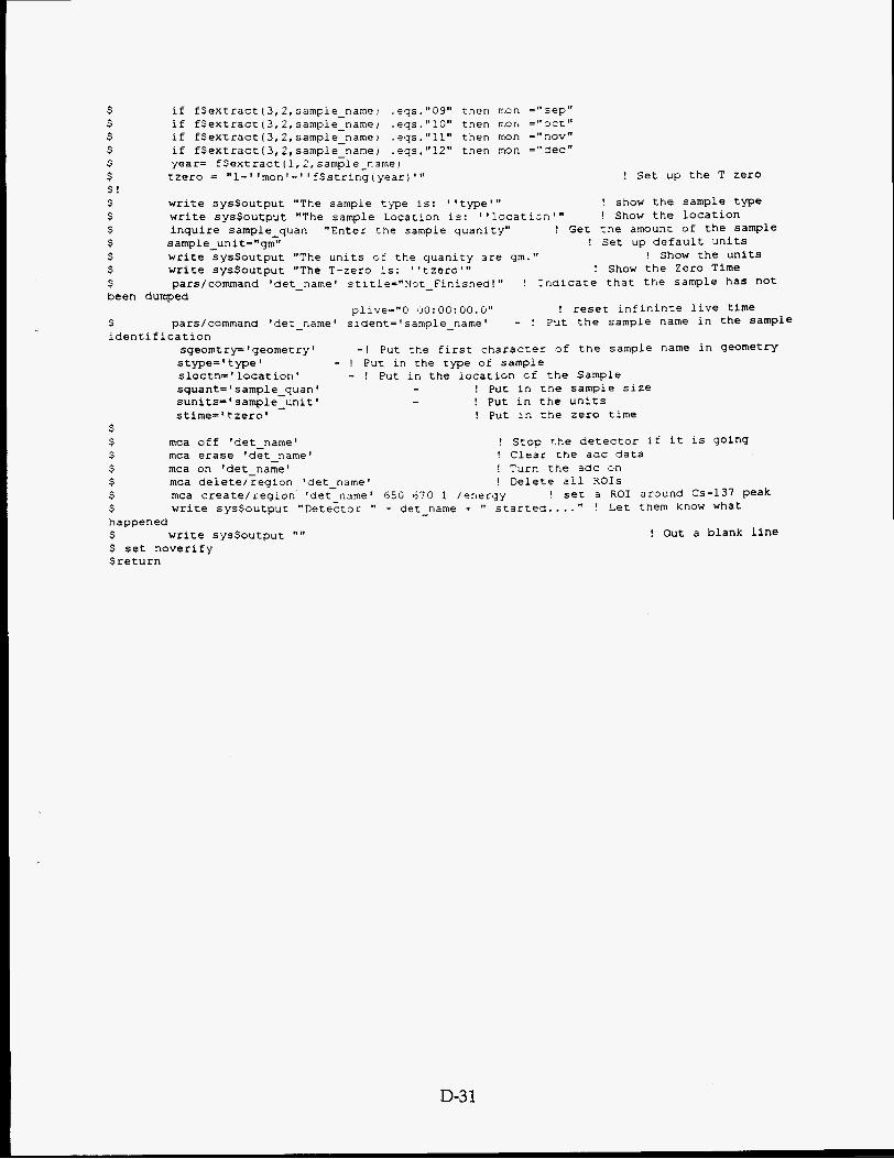
if fSextract (3,2,sample_name~ .eqs."09" then ran ="seF" if f S e x t r a c t ( 3 , 2 , s a m p l e _ n a m e l .eqs."lO" tnen non = " 3 c t " if fSextract ( 3 , 2 , sample-name I .eqs ."11" then mon ="nOV"

if fSextract(3,2,sample-name~ .eqs."l2" then ncIn ="iec" year= fSextract (1,2,sample_narne) t ze r o = " 1 - I ' mo n I - f $ s t r i nq ( ye a r ) ' I' ! Set up the T zero

! show the sample type write sysSoutput "The sample type is: "type'" ! Show the location write sysSoutput "The sample Location is: lllocatiza'"

inquire sample-quan "Enter cne sample quanity" ! Get the amount of the sample ! Set up default units s amp1 e-un i t="qm"

write SysSoutput "The units G F the quanity a re gm." write sysSoutput "The T-zero is: "tzero"' ! Show the Zero Time pars/command 'det-name' stitle="Not_Pinished!" ! Indicate that the sample ha= not

! show the units

been dumped

$ pars/command 'det-name' identification

sgeomtry='geometry' stype='type' - sloctn='location' squant='sample-quan' sunits='sample-unit' stimef'tzero'

S

plive="O 3O:OO:OO.O" ! resec infin sident='sample-name' - ! Put the sample

- ! Put the first character of the sample ! Put in the type of sample - ! Put in the location r,f The Sample - ! Put in che sample size

- ! Put in the units ! Put in =he zero time

nte name

name

ive time in the sample

in geometry

$ rnca off 'det-name' ! Stop ?he detector if it is going $ rnca erase 'det-name' ! Clear the adc data $ rnca on 'det-name' ! Turn ?Fie adc on $ rnca delete/region 'Jet-name' ! Delef-e a l l 301s $ rnca create/region' 'det-name' 650 670 1 / e n e r g y ! set 3 ROI around Cs-137 peak $ write sysSoutpuc "Detector 'I + aet-name t scarce2 ...." ! Let them know what happened S write sysSoutput "I' ! Out a blank line S set noverify $return

D-3 1

Appendix E -- Results an Initial Calibration

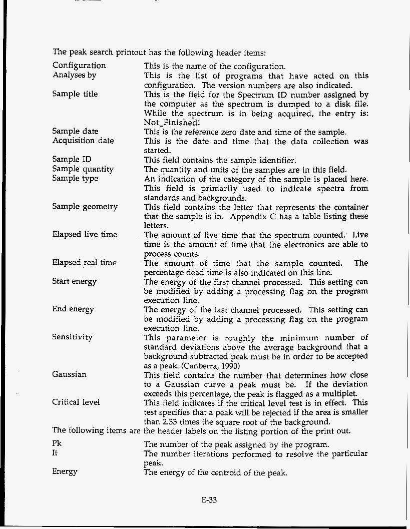
The peak search printout has the following header items: Configuration Analyses by

Sample title

Sample date Acquisition date

Sample ID Sample quantity Sample type

Sample geometry

Elapsed live time

Elapsed real time

Start energy

End energy

Sensitivity

Gaussian

Critical level

This is the name of the configuration. This is the list of programs that have acted on this configuration. The version numbers are also indicated. This is the field for the Spectrum ID number assigned by the computer as the spectrum is dumped to a disk file. While the spectrum is in being acquired, the entry is: No t-Finished! This is the reference zero date and time of the sample. This is the date and time that the data collection was started. This field contains the sample identifier. The quantity and units of the samples are in this field. An indication of the category of the sample is placed here. This field is primarily used to indicate spectra from standards and backgrounds. This field contains the letter that represents the container that the sample is in. Appendix C has a table listing these letters. The amount of live time that the spectrum counted.’ Live time is the amount of time that the electronics are able to process counts. The amount of time that the sample counted. The percentage dead time is also indicated on this line. The energy of the first channel processed. This setting can be modified by adding a processing flag on the program execution line. The energy of the last channel processed. This setting can be modified by adding a processing flag on the program execution line. This parameter is roughly the minimum number of standard deviations above the average background that a background subtracted peak must be in order to be accepted as a peak. (Canberra, 1990) This field contains the number that determines how close to a Gaussian curve a peak must be. If the deviation exceeds this percentage, the peak is flagged as a multiplet. This field indicates if the critical level test is in effect. This test specifies that a peak will be rejected if the area is smaller than 2.33 times the square root of the background.

The number of the peak assigned by the program. The number iterations performed to resolve the particular peak. The energy of the centroid of the peak.

The following items are the header labels on the listing portion of the print out. Pk It

Energy

E-33

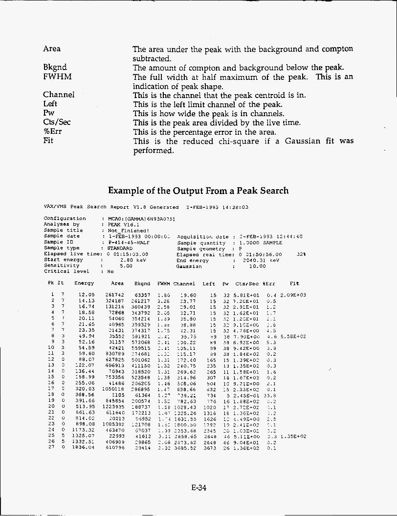
Area

Bkgnd FWHM

Channel Left Pw CtS/SeC %Err Fit

The area under the peak with the background and compton subtracted. The amount of compton and background below the peak. The full width at half maximum of the peak. This is an indication of peak shape. This is the channel that the peak centroid is in. This is the left limit channel of the peak. This is how wide the peak is in channels. This is the peak area divided by the live time. This is the percentage error in the area. This is the reduced chi-square if a Gaussian fit was performed.

Example of the Output From a Peak Search VAX/VMS Peak Search Report V1.8 GeneraTed 2-FEB-1993 14:38:03

Conf igurat ion : MCAO: [GAMMA] 6H93AOlSl Analyses by : PEAK V16.1 Sample t i t l e : Not-Finished! Sample d a t e : 1-FEB-1993 0O:OO:G; A c q u i s i t i o n d a t e : 2-TEB-1993 12:44:40 Sample ID : P-414-45-HALF Sample q u a n t i t y : 1.0000 SAMPLE Sample type : STANDARD Sample geometry : P Elapsed l i v e t ime: 0 01:15:03.00 Elapsed r e a l t i m e : 0 21:50:56.00 32% S t a r t energy S e n s i t i v i t y C r i t i c a l l e v e l

Pk I t

1 7 2 7 3 7 4 7 5 7 6 7 7 7 8 3 9 3 10 3 11 3 12 0 13 0 14 0 15 0 16 0 17 0 18 0 19 0 20 0 21 0 22 0 23 0 24 0 25 5 26 5

Energy

12.05 14.13 16.74 18.58 20.11 21.65 23.35 49.94 52.16 54.59 59.60 88.07

122.07 136.44 158.99 255.06 320.03 368.56 391.66 513.95 661.63 814.02 898.08

1173.32 1325.07 1332.51

2.80 k e V End energy : 2040.31 k e V 5.00 Gaussian 10.00

: N o

Area Bkgnd

261742 63357 324187 261217 131216 360439 72868 343792 54060 354214 40965 399329 21431 374317 35552 581921 31157 572068 42421 559515

830789 274681 627825 501062 606913 411150 70943 318520

753356 523548 41486 206205

1050118 286895 1105 61364

845854 200574 1223935 188737 611640 173213 20213 56952

1085392 121708 163470 67037 22993 41612

406909 -9865

EWHH Channel

i . a o l9.60 3.2E 23.77 2.5& 29.01 2.55 32.71

1 . z ~ 32 .88 1 . 7 5 42.31 2 . 4 : 35.75 2 . 4 ; 130.22 2 . 4 ; 105.11 1.5: li5.17 1.3: 172.40 1 .32 240.75 1.3: 269.62 l.3E 314.96 1.46 538.06 1.47 638.66 1.2? '36.21 1 .52 782.63 1.53 1028.43 1.6- 1335.26 1.-; 1631.55 1.5: 1800.50 1.3.2 2353.68 3.1: 2658.65 2.G3 2673.62

* . - > 1 2 5 35-80 . - -

L e f t Pw C t s i S e c %Err F i t

15 32 5.812+01 15 32 7.20E+01 15 32 2.91E+01 15 32 1.62E-01

15 32 9 . l E : c O G

89 ja ~ . ~ G Z + O G ug 3 a 6.92~+00

15 3 2 1 . 2 C ~ T 0 1

15 32 4.76Z+OO

89 38 9.42E+OO 89 38 1 .84Et02 165 15 1.39E+O2 235 13 1.35S+02 265 11 1.58E+01 307 16 1.672+02 504 10 9.212+00 v32 15 2.335+02 734 5 2.45@-01 776 16 1.6eE-02 1020 17 2.72E+02 1316 1s 1.35E+02 1626 1: 4 . 4 9 5 + 0 0 1792 13 2.41s-02 2345 26 1.032+02 2648 46 5.115+00 2648 46 9.04E-01

0.4 2.09E+03 0.5 1.2 1.7 2.1 2 . 8 4.5 4 . 6 5.5EE+02 5.3 3.9 0 . 2 a.3 0.3 1.6 0.2 2.1 3.1

33.8 u.2 3.1 1.2 1 .5 2.1 j.2 2.3 1.35E+02 0.2

27 0 1836.04 610796 29414 2 . 3 1 3685.52 3 6 7 3 26 1.36't+O7- 0.1

E-34

Appendix F -- Results of an Update Calibration

The peak search printout has the following header items:

Configuration Analyses by

Detector Name

Energy Calib Time

Efficiency type

Effncy Calib Time

Detector Geometry Shelf

This is the name of the configuration. This is the list of programs that have acted on this configuration. The version numbers are also indicated. This is the designator of the detector the sample was counted on. This is the date and time that the energy calibration used for the calculation was performed. This field indicates the type of calibration. The two possible types are empirical or non-empirical. This is the date and time that the efficiency calibration used for the calculation was performed This field describes the calibration in abbreviated notation. This field is not used. Its purpose is to indicate the distance the sample is with respect to the detector window.

The Energy Calibration Report section contains the following:

An equation describing the energy - channel relationship.

Nbr Centroid Channel True Energy

Computed Energy

Difference

The number of the standard peak. The channel that the centroid of the peak resides in. The energy of the peak centroid as indicated in the certificate file The energy the program computed from the calculated equation. The result from subtracting the computed energy from the certificate energy.

The Efficiency Calibratiorz Report portion of the report contains: The equation that describes the efficiency curve, if an empirical calibration is being calculated, followed by the calculated coefficients. Average Deviation = This is a measure of uncertainty in the calculated fit. Reduced Chi-square = This is a measure of uncertainty in the calculated fit. The following items are reported for each peak described in the certificate file. Nbr This is the number of the Standard peak. Energy This is the energy measured in keV of the peak as recorded

in the certificate file. -

Measured Efficiency This is the efficiency for the particular peak calculated from the spectra.

Efficiency Error This is the calculated error in the efficiency.

F-36 I

Computed Efficiency

Diff/ Error

% Diff

This is the efficiency for the particular peak calculated from the fit. This is the measured efficiency subtracted from the calculated efficiency and then divided by the efficiency error. The is the percentage difference between the measured efficiency and the calculated efficiency.

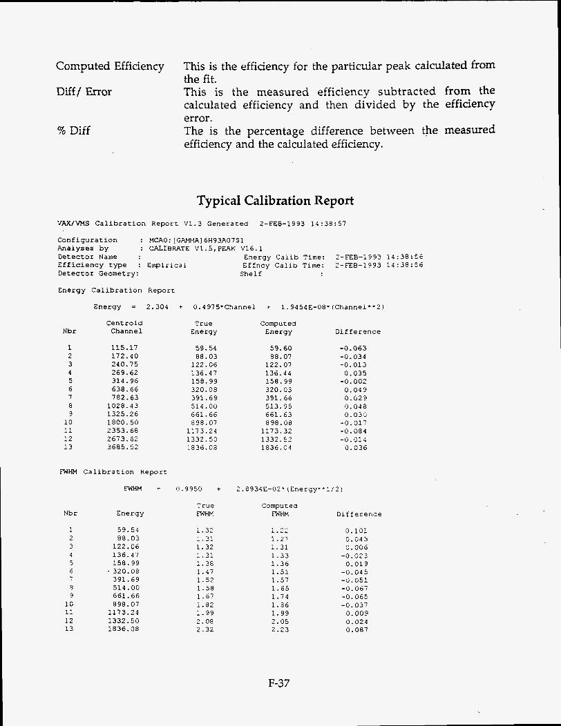
Typical Calibration Report VAX/VMS Calibration Report V1.3 Generated 2-FEB-1993 14:38:57

Configuration : MCAO: [GAMMA] 6H93A07Sl Analyses by : CALIBRATE V1.5,PEAK V16.1 Detector Name Energy Calib Time: 2-FEb-1993 14:38:56 Efficiency type : Empirical Effncy Calib Time: 2-FEE-1993 14:38:56 Detector Geometry: Shelf

Energy Calibration Report

Energy = 2.304 + 0.4975*Channel + 1.9454E-O8*(Channei**2)

Nbr

1 2 3 4 5 6 7 e 9

10 11 12 13

Centroid Channel

115.17 172.40 240.75 269.62 314.96 638.66 782.63 1028.43 1325.26 1800.50 2353.68 2673.62 3685.52

True Energy

59.54 88.03 122.06 136.47 158.99 320.08 391.69 514.00 661.66 898.07 1173.24 1332.50 1836.08

Computed Energy

59.60 88.07 122.07 136.44 158.99 320.03 391.66 513.95 661.63 898.08 1173.32 1332.52 1836.04

Difference

FiiHM Calibration Report

FWHM = 0.9950 + ~.8934E-l~2f(Energy**l/2)

-0.063 -0.034 -0.013 0.035 -0.002 0.049 0.023 9.048 0.03:: -0.01- -0.084 -0.01 4 0.036

Nbr

2

4 5 6 7 9 9 10 11 12 13

d

Enerqy

59.54 88.03 122.06 136.47 158.99

. 320.08 391.69 514.00 661.66 898.07 1173.24 1332.50 1836.08

True EWHM

1.32 1.31 1.32 1.31 1.38 1.47 1.52 1.58 1.67 1.82 1.99 2.08 2.32

Compu TI ea FWHM

1.2: 1 .27 1.31 1.33 1.36 1.51 1.57 1.65 1.74 1.86 1.99 2.05 2.23

Di f feren.ze

0.10: 0.045 0.006

- 0 . 0 2 3 0.019

-0.045 -0.05: -0.067 -0 .065 -0.037 0.009 0.029 0.087

F-37

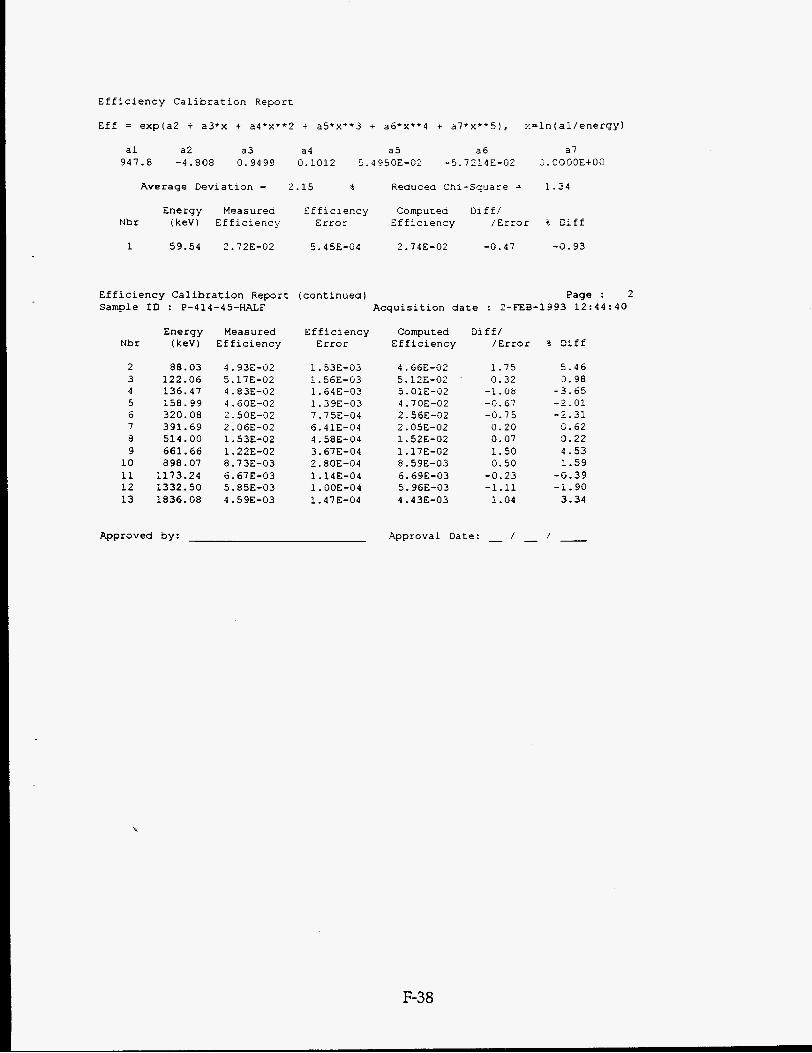
E f f i c i e n c y C a l i b r a t i o n Repor t

E f f = e x p ( a 2 + a3*x + a4*x**Z t a5*x**3 + a6*x+*4 + a 7 * x f * 5 ) , x = l n ( a l / e n e r g y )

a1 a2 a 3 a4 a 5 a 6 a7 947.8 -4.808 0.9499 0 .1012 5.4950E-02 -5.7214E-02 3.OCOOE+00

A v e r a g e D e v i a t i o n = 2 . 1 5 % Reduced Ch i - squa re = 1.34

Energy Measurea E f f i c i e n c y Computed D i f f l Nbr ( k e V 1 E f f i c i e n c y E r r o r E f f i c i e n c y / E r r o r I 2 i f f

1 59.54 2.72E-02 5.45E-04 2 .7 4E-02 -0.47 - 5 . 9 3

E f f i c i e n c y C a l i b r a t i o n Repor t ( c o n t i n u e d ) Page : 2 Sample I D : P-414-45-HALF A c q u i s i t i o n d a t e : 2-FEB-1993 12:44:40

Energy Measured E f f i c i e n c y Computed D i f f / N b r (keV1 E f f i c i e n c y E r r o r E f f i c i e n c y /Error % D i f f

2 88 .03 4.93E-02 3 122.06 5.17E-02 4 136.47 4.83E-02 5 158 .99 4.60E-02 6 320 .08 2.50E-02 7 391.69 2.066-02 8 514.00 1.53E-02 9 661.66 1.22E-02

1 0 898 .07 8.73E-03 11 1173.24 6.67E-03 1 2 1332.50 5.858-03 13 1836.08 4.59E-03

1.53E-03 1.56E-03 1.64E-03 1.39E-03 7.75E-04 6.41E-04 4.58E-04 3.67E-04 2.80E-04 1.14E-04 1.008-04 1.41 E-04

4.66E-02 5.12E-02 5.01E-02 4.708-02 2.56E-02 2.05E-02 1.52E-02 1.17E-02 8.59E-03 6.696-03 5.96E-03 4.43E-03

1 . 7 5 0 .32

-1.08 -0.67 -0.75

0 .20 0.07 1.50 0.50

-0 .23 -1.11

1.04

5 .46 3.98

-3 .65 -2.01 -5.31

0.62 3.22 4.53 1 . 5 9

-0 .39 -i. 90 3.34

Approved by: Approval Date : - / - / -

F-38

Appendix G -- Data Handling Codes and Databases

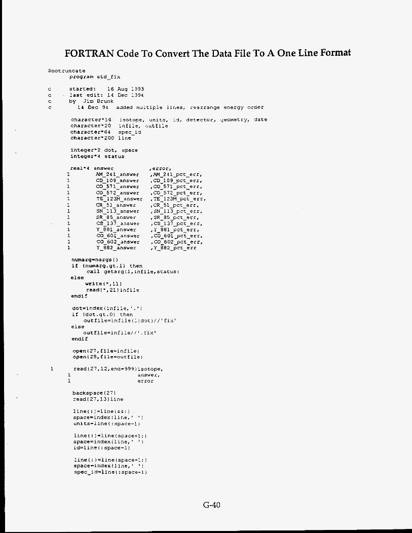
FORTRAN Code To Convert The Data File To A One Line Format Snotruncate

program std-fix

started: 16 Aug 1993 last edit: 14 Dec 1994 by J1m Brunk

14 Dec 94 added multiple lines, rearrange energy order

1 1 1

C C C C

character*l6 isotope, units, id, det-ector, geometry, date characrerc20 infile, outfile character* 64 spec-id character*200 line

integer*2 dot, space integer'4 status

real'4 1 1 1 1 1 1 1 1 1 1 1 1 1

answer AM-24 1-answer CD-109-answer CO-57 1-answer CO-57 2-answer TE-123M-answer CR-51-answer SN-113-answer SR-85-answer CS-137-answer Y-88l-answer CO-601-answer C0-602-answer Y-882-answer

,error, ,AM-241-pct-erz, , CD-lO9-pct-err, ,C0-57l-pct-err, ,C0-572-pct-err, ,TE-123M-pct-err, ,CR-Sl-pct-err, ,SN-l13pct_err, ,SR-85-pct-err, ,CS-137-pct-err ,Y_88l_pct_err, ,C0_60l_pct_err ,CO-602-pct-err , Y-882-pct-err

numarg=nargs ( ) if (numarg.gt.1) then

else call getarg(l,infile,status)

write (*, 11 I read[*,Zl)infile

endif

dot=index(infi:e, ' . ' ) if (dot.yt.0) chen

else

endi f

outfile=infile(l :dot ) / / fix'

outfile=infile//' .fix'

read (27,12, end=999 isotope, answer, error

backsDace(27) read(27,13)line

line(:)=line(44:) space=index(line,' ' ) units=line(:space-1)

line(:)=line(space+l:) space=index(lice, ' ' ) id=line ( : space-1 I

line(: )=line(space+l:) space=index (line, ' ' ) spec-id=line(:space-l)

G-40

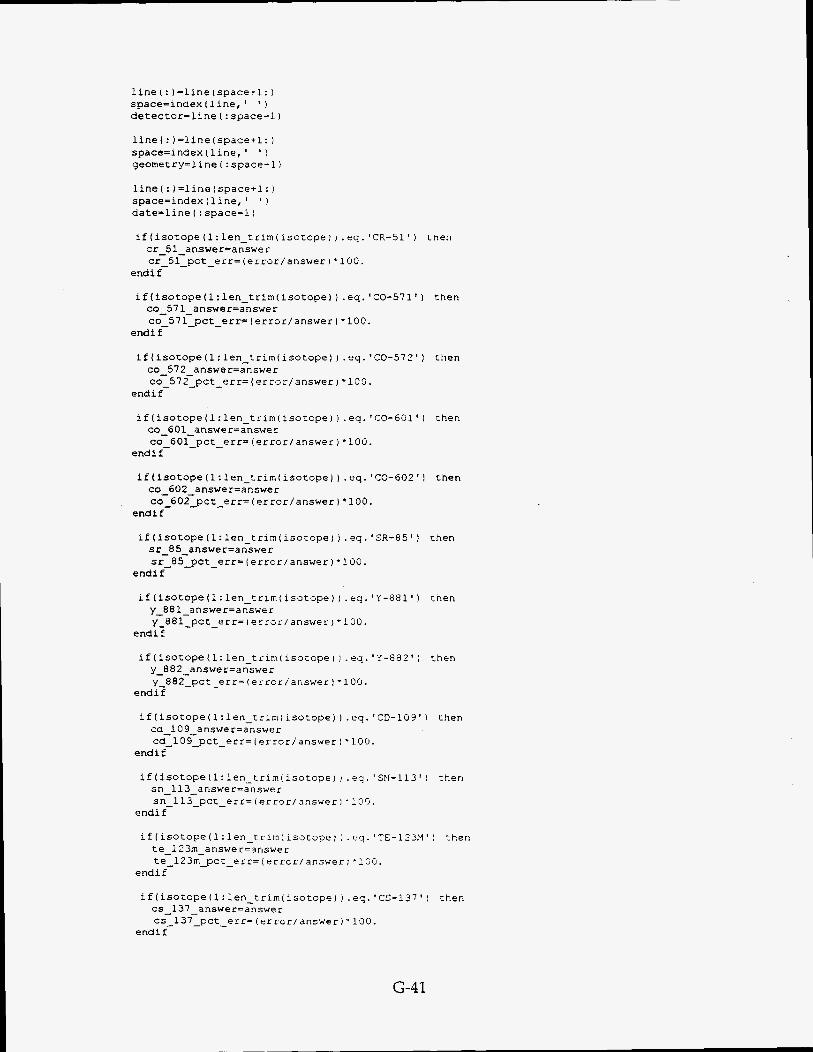
line(:)=line(space+l:) space=index(line,' ' ) detector=line(:space-1)

line(:)=line(space+l:) space=index(line, ' ' 1 geometry=line ( : space-1)

line(:)=line(space+l:) space=index(line, * ! date=line(:space-1)

if(isotope(l:len-trim(isotope)i.eq.'CR-51t) tnen cr-5l-answer=answer cr-5l-pct-err=(error/answer)+lOO.

endif

if (isotope (1: len-trim(isotope) ) . eq. 'CO-571' ) then co-57l-answer=answer co~57l~pct~err=(error/answer)*lOO.

endi f

if(isotope(l:len-trim(isotope)J.eq,'CO-572') then co_572_answer=answer co~572~pct~err=(error/answer)*lOC1.

endi f

if(isotope(l:len-trirn(isotope)).eq.'C3-601') then co-6Ol-answer=answer co~60l~pct~err=(error/answer1*100.

endif

if(isotope(l:len-trirn(isotope)).eq.'CO-602'1 then co-602-answer=answer co-602-pct-err=(error/answer1*1OO.

endi f

if(isotope(l:len-trim(isotope)j.eq.'SR-85') then sr-85-answer=answer sr-85-pct-err=(error/answer)*lOO.

endi f

if(isotope(l:len-trim(isotope)i.eq.'Y-Y81') tnen y-EBl-answer=answer y-88l-pct-err=(error/answer)c100.

endi f

if (isotope ( 1 : len-t rim( isotope i I . eq. "1'-88 2' I then y-882-answer=answer y-882-pct-e r r= ( e r ror / answer 1 * 1 00.

endif

if(isotope(l:len-trirn(isotope) ).eq.'CD-103') then cd_lO9_answer=answer cd_l09-pct-err=(error/answer1'100.

endif

if (isotope (1: len-trirn( isotope) ) . "1. 'SN-113' ) then sn_ll3_answer=answer sn-ll3-pct-err=(error/snswer)*lO'J.

endi f

i f ( i s o t o p e ( l : l e n - t r i m ( i s a r o p e ) t t e-1 2 3m-answe r=arIswe r t e_123rngc t_e r r= (e r ro r / answer

endi f

if (isotope (1 : len-trirn(isotope) ) cs-l37_answer=answer cs-l37_pct_err= (erroriansweri

endif

eq. 'TE-123M' ) then

'150.

eq.'CS-137'1 then

100.

G-41

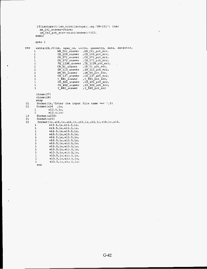
if(isotope!1:1en-trim(isotope)).eq.8PM-241') then am-24l-answer=answer am-24l-pct-err=(error/answer)*100.

endif

,

got0 1

999 write(28,22) id, spec-id, units, geometry, date, detectcr. 1 AM-24l-answer ,;\M_24l_pct_err, 1 CD-109-answer ,CD_109_pct_err, 1 C0-57l-answer ,C0_57l_pct_err, 1 C0-572-answer ,CO_572_pct_err, 1 TE-123M-answer ,TE_123M_pct_err, 1 CR-51-answer ,CR_51_pct_err, 1 SN-113-answer ,SN_ll3_pct_err, 1 SR-85-answer ,SR_85_Gct_err, 1 CS-137-answer ,CS_137_pct_err, 1 Y-EBl-answer ,Y-881-pctderr, 1 C0-60l-answer ,CO-6Ol-pct-err, 1 C0-602-answer ,CO_602-pct-err, 1 Y-882-answer ,Y_882_pct_err

close (27 ) close (28 1 stop

11 format(lx,'Enter the input file name ==> ',$) 12 format(al6 ,lx,

1 e12.4, lx, 1 e12.4, lx)

13 format (a2001 21 format(a20) 22 format (lx, 516, lx, ab4, l x , alG, lx, a16, l x , 3.16, lx, 316,

1 e13.5, lx, e13.5, lx, 1 e13.5, lx, e13.5, lx, 1 e13.5,lx,e13.5,1~, 1 e13.5,lx,e13.5,1~, 1 e13.5,lx,e13.5, lx, 1 e13.5,lx,e13.5, lx, 1 e13.5,lx,e13.5,1~, 1 e13.5,lx,e13.5, lx, 1 e13.5,1x,e13.5,1~, 1 e13.5,1xf e13.5, lx, 1 e13.5, lx, e13.5, lx, 1 e13.5,lx,el3.5,1~, 1 e13.5,lx,e1~.5,1x) end

G-42

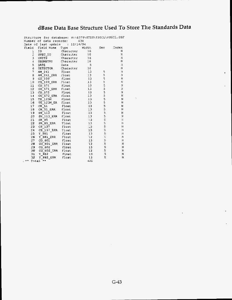
dBase Data Base Structure Used To Store The Standards Data S t r u r r u r e for d a t a b a s e : H: \0379\STDS\FSOIL\FSCIL. DBF Number of d a t a records: 4 3 4 Date of l a s t u p d a t e : 12/14/94 F i e l d F i e l d N a m e

I I D 2 SPEC-ID 3 UNITS i GEOMETRY 5 DATE 6 DETECTOR

3 AM-241 ERR 3 CD-109-

10 CD-10 9-ERR 11 CO-571 12 CO-57 1-ERR 13 CO-572 14 CO-57 2-ERR 15 TE-123M 16 TE-123M-ER 17 CR-51 18 CR-51-ERR 19 SN-113 2 0 SN-113-ERR 2 1 SR-85 2 2 SR-85-ERR 2 3 CS-137 24 CS-137-ERR

2 6 Y-881-ERR 27 CO-601 2 8 C0-601-ERR 2 9 CO-602 3 0 C0-602-ERR 31 Y-882 32 Y-882-ERR

7 AM-241

2 s Y-881

* * T c z a l **

Type Width C h a r a c t e r 1 6 C h a r a c t e r 10 C h a r a c t e r 16 C h a r a c t e r 1 6 Date 8 C h a r a c t e r 16 F l o a t 13 F l o a t 13 F l o a t 13

13 : l o a t F l o a t 13 F l o a t 13 F l o a t 13 F l o a t 13 F l o a t 13 F l o a t 13 F loa t 13 F l o a t 13 F l o a t 13 F l o a t 13 F l o a t 13 F l o a t 1 3 F lGat 13 F l o a t 13 F l o a t 13 F l o a t 13 F l o a t 13 F l o a t 13 F l o a t 13 F l o a t 13 F l o a t 13 F l o a t 13

421

- 7

Dec i n d e x N N N N tJ N

5 N 5 N 5 N 5 f l 4 N 5 N 5 N 5 N 5 N 5 N 5 N 5 N 5 N 5 N 5 N 5 N 5 N 5 N 5 Pl ., N 5 N 5 N 5 N 5 N 5 N 5 N

c

G 4 3