Embed Size (px)
Citation preview

UCLA workshop June 2005 1
ISSUES IN BOUNDARY LAYER PARAMETRIZATION FOR LARGE SCALE MODELS
Anton Beljaars*(ECMWF)
• Boundary layer clouds
• Wind turning
• Momentum budget (heterogeneous terrain)
•With contributions from: Andy Brown, Sylvain Cheinet, Hans Hersbach, Martin Koehler, Andrew Orr

UCLA workshop June 2005 2
Recent implementation of Mass-flux/K-diffusion approach
key ingredients:
• moist conserved variables
• combined Mass-flux/K-diffusion solver
• cloud variability
• transition between stratocumulus and shallow convection

UCLA workshop June 2005 3
Results: Low cloud cover (new-old)
T511 time=10d
n=1402001 & 2004
old: CY28R4 new PBL

UCLA workshop June 2005 4
Results: EPIC column extracted from 3D forecasts
Liquid Water Path [g/m2]
16 17 18 19 20 21 22Local Time [October 2001 days]
0
50
100
150
200
250
300
old PBLnew MK PBLEPIC obs
WV Mixing Ratio [g/kg]
0 2 4 6 8 10
1000
950
900
850
800
750
700
Pre
ssur
e [h
Pa]
Mod
el L
evel
s
45
50
55
60

UCLA workshop June 2005 5
ARM SGP, number of cloudy hours in July 2003
Cloud radar Model
Model lacks afternoon shallow cumulus
Sylvain Cheinet (2005)

UCLA workshop June 2005 6
ARM SGP, daily 36 hr back trajectories, July 2003
L42, 600 hPa
L54, 950 hPa
Cross section of model moisture and cloud cover for fair weather days in July 2003 (q: shaded; cc: contours at 0.01, 0.02, 0.05)

UCLA workshop June 2005 7
ARM SGP, surface fluxes (model/obs)
HLE
Monthly domain averaged diurnal cycle
West-East change of LE/H
Time evolution of LE and H for station C1

UCLA workshop June 2005 8
ARM SGP, 2m T/q, BL wind (model/obs)
28R1 28R1 +MO stable BL

UCLA workshop June 2005 9
ARM SGP: Sensitivity to shallow convection
Cross section of model humidity difference for fair weather days in July 2003 (Effect of No Shallow Convection)
Cross section of model humidity difference for fair weather days in July 2003 (Effect of halving shallow convection mass flux over land)

UCLA workshop June 2005 10
Boundary layer cloud issues
•The switching algorithm is unsatisfactory. Unification between stratocumulus and shallow cumulus is desirable. What is the physical mechanism that controls the regime?
•Numerics of inversion handling
•Cloud top entrainment?
•Closure for shallow convection?
•Does a scheme have the correct feedbacks and how can we test this?
•What is the role of shallow convection in more complicated situations (cold air outflow, momentum transport)

UCLA workshop June 2005 11
Geostrophic drag law
B
u
V
A
zf
u
u
U
G
om
G
*
*
*
)ln(1
drag
a-geostrophic angle
Wangara data

UCLA workshop June 2005 12
Operational verification of surface wind
A-geostrophic angle is too small

UCLA workshop June 2005 13
Operational verification of surface wind
Wind speed is too low during the day and too high at night

UCLA workshop June 2005 17
Examples of ERA40 forecast veers
260
264
264
264
268
268
268
272
272
272
276
276
276
280
280
284
284
288
288
25.0m/s
40°N40°N
50°N 50°N
60°N60°N
70°N 70°N
60°W
60°W 50°W
50°W 40°W
40°W 30°W
30°W 20°W
20°W 10°W
10°W 0°
0°
2002021312+24 level 55 T and wind
235.9
238
242
246
250
254
258
262
266
270
274
278
282
286
290
293.5
-12
-12
-12
-12
27
27
27
27
27
27
40°N40°N
50°N 50°N
60°N60°N
70°N 70°N
60°W
60°W 50°W
50°W 40°W
40°W 30°W
30°W 20°W
20°W 10°W
10°W 0°
0°
2002021312+24 surface to 850 hPa veer
-180
-27
-12
12
27
180
256260
260
264
264
268
268
268
268272
272
272
276
276
276
280
280
284
284
288
288
25.0m/s
40°N40°N
50°N 50°N
60°N60°N
70°N 70°N
60°W
60°W 50°W
50°W 40°W
40°W 30°W
30°W 20°W
20°W 10°W
10°W 0°
0°
2002021412+24 level 55 T and wind
237.7
240
244
248
252
256
260
264
268
272
276
280
284
288
292
294.0
-12
-12
-12
-12
-12
-12
-12
27
27 27
27
27
27
40°N40°N
50°N 50°N
60°N60°N
70°N 70°N
60°W
60°W 50°W
50°W 40°W
40°W 30°W
30°W 20°W
20°W 10°W
10°W 0°
0°
2002021412+24 surface to 850 hPa veer
-180
-27
-12
12
27
180
250m T andwind
Surface to 850 hPa veer >27o
12o27o
<-27o
-27o-12o
-12o12o
Veering in warm sectorof depression
Backing on and behindcold front
20020213 12Z+24 20020214 12Z+24
Brown et al. 2005

UCLA workshop June 2005 18
Atlantic sonde stations
• SST, December 1987
278
294
32°N32°N
34°N 34°N
36°N36°N
38°N 38°N
40°N40°N
42°N 42°N
44°N44°N
46°N 46°N
48°N48°N
50°N 50°N
52°N52°N
54°N 54°N
56°N56°N
58°N 58°N
60°N60°N
62°N 62°N
64°N64°N
66°N 66°N
68°N68°N
70°N 70°N
72°N72°N
74°N 74°N
76°N76°N
78°N 78°N
68°W
68°W
64°W
64°W
60°W
60°W
56°W
56°W
52°W
52°W
48°W
48°W
44°W
44°W
40°W
40°W
36°W
36°W
32°W
32°W
28°W
28°W
24°W
24°W
20°W
20°W
16°W
16°W
12°W
12°W
8°W
8°W
4°W
4°W
0°
0°
4°E
4°E
8°E
8°E
ECMWF Mean of 31 Uninitialised Analyses Valid: VT:00UTC 1 December 1987 to 00UTC 31 December 1987 Surface: sea surface temperature
271.0 274 277 280 283 286 289 292 295
SABLE
CHARLIE
LIMA
MIKE

UCLA workshop June 2005 19
SABLE (All points)
-50 0 50Sonde veer (degrees)
-50
0
50
For
ecas
t vee
r (d
egre
es) N=243
SCA CA NA WA SWA
SABLE (Stable points)
-50 0 50Sonde veer (degrees)
-50
0
50
For
ecas
t vee
r (d
egre
es) N=57
SCA CA NA WA SWA
CHARLIE (All points)
-50 0 50Sonde veer (degrees)
-50
0
50
For
ecas
t vee
r (d
egre
es) N=266
SCA CA NA WA SWA
CHARLIE (Stable points)
-50 0 50Sonde veer (degrees)
-50
0
50F
orec
ast v
eer
(deg
rees
) N=82
SCA CA NA WA SWA
LIMA (All points)
-50 0 50Sonde veer (degrees)
-50
0
50
For
ecas
t vee
r (d
egre
es) N=246
SCA CA NA WA SWA
LIMA (Stable points)
-50 0 50Sonde veer (degrees)
-50
0
50
For
ecas
t vee
r (d
egre
es) N=38
SCA CA NA WA SWA
MIKE (All points)
-50 0 50Sonde veer (degrees)
-50
0
50
For
ecas
t vee
r (d
egre
es) N=236
SCA CA NA WA SWA
MIKE (Stable points)
-50 0 50Sonde veer (degrees)
-50
0
50
For
ecas
t vee
r (d
egre
es) N=14
SCA CA NA WA SWA
SABLE (All points)
-50 0 50Sonde veer (degrees)
-50
0
50
For
ecas
t vee
r (d
egre
es) N=243
SCA CA NA WA SWA
SABLE (Stable points)
-50 0 50Sonde veer (degrees)
-50
0
50
For
ecas
t vee
r (d
egre
es) N=57
SCA CA NA WA SWA
CHARLIE (All points)
-50 0 50Sonde veer (degrees)
-50
0
50
For
ecas
t vee
r (d
egre
es) N=266
SCA CA NA WA SWA
CHARLIE (Stable points)
-50 0 50Sonde veer (degrees)
-50
0
50
For
ecas
t vee
r (d
egre
es) N=82
SCA CA NA WA SWA
LIMA (All points)
-50 0 50Sonde veer (degrees)
-50
0
50
For
ecas
t vee
r (d
egre
es) N=246
SCA CA NA WA SWA
LIMA (Stable points)
-50 0 50Sonde veer (degrees)
-50
0
50
For
ecas
t vee
r (d
egre
es) N=38
SCA CA NA WA SWA
MIKE (All points)
-50 0 50Sonde veer (degrees)
-50
0
50
For
ecas
t vee
r (d
egre
es) N=236
SCA CA NA WA SWA
MIKE (Stable points)
-50 0 50Sonde veer (degrees)
-50
0
50
For
ecas
t vee
r (d
egre
es) N=14
SCA CA NA WA SWA
Veering between surface (10m) and 850 hPa wind: comparison of 24 hour ERA40 forecast with 12Z sonde

UCLA workshop June 2005 20
Composite ERA40 results(4 winters; Sable, Charlie, Lima and Mike combined)
• When sonde shows big veering, model veers less
• When model shows big veering, sonde veers more– Model definitely under-veers
• When sonde shows big backing, model backs less
• When model shows big backing, sonde veers are similar– Model probably under-backs
Surface to 850 hPa
-50 0 50Sonde veer (deg.)
-50
0
50
For
ecas
t vee
r (
deg.
)
Categories by sonde veerCategories by forecast veer
8310121843210849
32
49
240
597
50
23
850 hPa to 700 hPa
-50 0 50Sonde veer (deg.)
-50
0
50
For
ecas
t vee
r (
deg.
)
Categories by sonde veerCategories by forecast veer
254511564715676
34
37
120
675
144
54
UCLA workshop June 2005 21
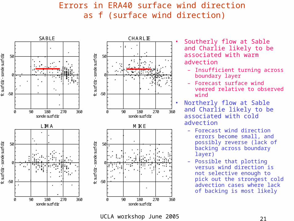
Errors in ERA40 surface wind direction as f (surface wind direction)
• Southerly flow at Sable and Charlie likely to be associated with warm advection
– Insufficient turning across boundary layer
– Forecast surface wind veered relative to observed wind
• Northerly flow at Sable and Charlie likely to be associated with cold advection
– Forecast wind direction errors become small, and possibly reverse (lack of backing across boundary layer)
– Possible that plotting versus wind direction is not selective enough to pick out the strongest cold advection cases where lack of backing is most likely
SABLE
0 90 180 270 360sonde surf dir
-50
0
50
fc s
urf
dir
- so
nde
surf
dir
CHARLIE
0 90 180 270 360sonde surf dir
-50
0
50
fc s
urf
dir
- so
nde
surf
dir
LIMA
0 90 180 270 360sonde surf dir
-50
0
50
fc s
urf
dir
- so
nde
surf
dir
MIKE
0 90 180 270 360sonde surf dir
-50
0
50
fc s
urf
dir
- so
nde
surf
dir

UCLA workshop June 2005 22
Impact of resolution and model
• Qualitatively similar results in ECMWF T511 operational model and also in Met Office operational model
ERA40 DJF0002
-50 0 50Sonde veer (deg.)
-50
0
50
For
ecas
t ve
er
(deg
.)
Categories by sonde veerCategories by forecast veer
85961974522
31
124
257
23
10
ECMWF DJF0002
-50 0 50Sonde veer (deg.)
-50
0
50
For
ecas
t ve
er
(deg
.)
Categories by sonde veerCategories by forecast veer
85952014421
28
104
277
28
9
ECMWF DJF0304
-50 0 50Sonde veer (deg.)
-50
0
50
For
ecas
t ve
er
(deg
.)
Categories by sonde veerCategories by forecast veer
48621112315
22
65
154
15
3
MET OFFICE DJF0304
-50 0 50Sonde veer (deg.)
-50
0
50
For
ecas
t ve
er
(deg
.)
Categories by sonde veerCategories by forecast veer
48641092016
26
68
144
13
6

UCLA workshop June 2005 23
Stable boundary layer diffusion
Diffusion coefficients based on Monin Obukhov similarity:
2
2 )(
''
z
U
z
gRi
Riflz
UK
zKw

UCLA workshop June 2005 24
Impact of MOSBL on veers (1 winter; Sable, Charlie, Lima and Mike combined)
• Typically increased 5o in stable cases
• Further weakening of mixing by reducing length scale from 150m to 50m gives further small increase
UNSTABLE POINTS
-50 0 50sonde veer (deg.)
-20
-10
0
10
20
(mos
bl)-
(con
trol
) fo
reca
st v
eer
(de
g.)
SCA CA NA WA SWA
STABLE POINTS
-50 0 50sonde veer (deg.)
-20
-10
0
10
20
(mos
bl)-
(con
trol
) fo
reca
st v
eer
(de
g.)
SCA CA NA WA SWA

UCLA workshop June 2005 25
Wind direction from QuikSCAT

UCLA workshop June 2005 26
Wind direction
• Operational models underestimate a-geostrophic angle (what controls boundary layer veering?)
• Stable boundary layers do occur frequently over the ocean
• Real boundary layers are baroclinic (systematic LES simulations covering a wide range of baroclinicity may be helpful?)

UCLA workshop June 2005 29
Surface drag, momentum budget
• Surface drag is controlled by boundary layer mixing and surface roughness length
• Less boundary layer mixing (e.g. in stable boundary layer) leads to less surface drag
• Surface drag (or effective roughness) over land is very uncertain due to terrain heterogeneity effects

UCLA workshop June 2005 30
Z0-table

UCLA workshop June 2005 31
z0

UCLA workshop June 2005 32
CD-control

UCLA workshop June 2005 33
TOD+new z0 table

UCLA workshop June 2005 34
MO

UCLA workshop June 2005 35
ZM stress + Ps
Zonal mean West-East turb. stress Zonal mean surf. press. error (step=24)
ControlNew z0-table
ControlMO-stab.f.
ControlNew z0-table
ControlMO-stab.f.

UCLA workshop June 2005 36
Error tracking
Control
MO-stab.f.

UCLA workshop June 2005 37
500 hPa RMSerror NH,
200403
500 hPa activityDivided by
Analysis activity NH, 200403
ControlMO-stab.f.
ControlMO-stab.f.

UCLA workshop June 2005 38
500 hPa RMSerror NH,
200403 ControlNew z0-table
500 hPa activityDivided by
Analysis activity NH, 200403
ControlNew z0-table

UCLA workshop June 2005 39
BL-Veering
Control-New z0-table
Control
Control-MO

UCLA workshop June 2005 40
Conclusions
• NWP is sensitive to surface drag. Drag is affected by vegetation roughness, orographic effects and stability.
• It is difficult to verify surface drag.
• Roughness lengths are derived from land use data sets, without considering heterogeneity. Results are uncertain.
Research topics
• Derive geometric land use parameters from satellite data
• Run high resolution canopy resolving models to “measure” effective roughness length and its interaction with stability
• Infer surface drag from synoptic development (variational techniques that minimize short range forecast errors?)