Two Step Time Discretization of Willmore Flow

Nadine Olischlager and Martin Rumpf

Institut fur Numerische Simulation,Rheinische Friedrich-Wilhelms-Universitat Bonn,

Nussallee 15, 53115 Bonn, Germany{nadine.olischlaeger,martin.rumpf}@ins.uni-bonn.de,

WWW home page: http://numod.ins.uni-bonn.de/

Abstract. Based on a natural approach for the time discretization ofgradient flows a new time discretization for discrete Willmore flow ofpolygonal curves and triangulated surfaces is proposed. The approach isvariational and takes into account an approximation of the L2-distancebetween the surface at the current time step and the unknown surfaceat the new time step as well as a fully implicity approximation of theWillmore functional at the new time step. To evaluate the Willmoreenergy on the unknown surface of the next time step, we first ask forthe solution of a inner, secondary variational problem describing a timestep of mean curvature motion. The time discrete velocity deduced fromthe solution of the latter problem is regarded as an approximation ofthe mean curvature vector and enters the approximation of the actualWillmore functional. To solve the resulting nested variational problem ineach time step numerically relaxation theory from PDE constraint opti-mization are taken into account. The approach is applied to polygonalcurves and triangular surfaces and is independent of the co-dimension.Various numerical examples underline the stability of the new scheme,which enables time steps of the order of the spatial grid size.

1 Introduction

In this paper a new scheme for the time and space discretization of parametricWillmore flow is presented. Willmore flow is the L2 gradient flow of surfaces forthe Willmore energy, which measures the squared mean curvature on the surface.Let M be a closed d-dimensional surface embedded in Rm with m ≥ d + 1 anddenote by x the identity map on M = M[x]. Then the Willmore energy isdefined as

w[x] :=12

∫M

h2 da

where h is the mean curvature onM, i. e., h is the sum of the principle curvatureson M. Furthermore, the L2-metric

∫M v1v2 da measures variations x + vin of

the surface M in direction of the surface normal n. Given energy and metric thecorresponding gradient flow – the Willmore flow – in the hypersurface case (cf.

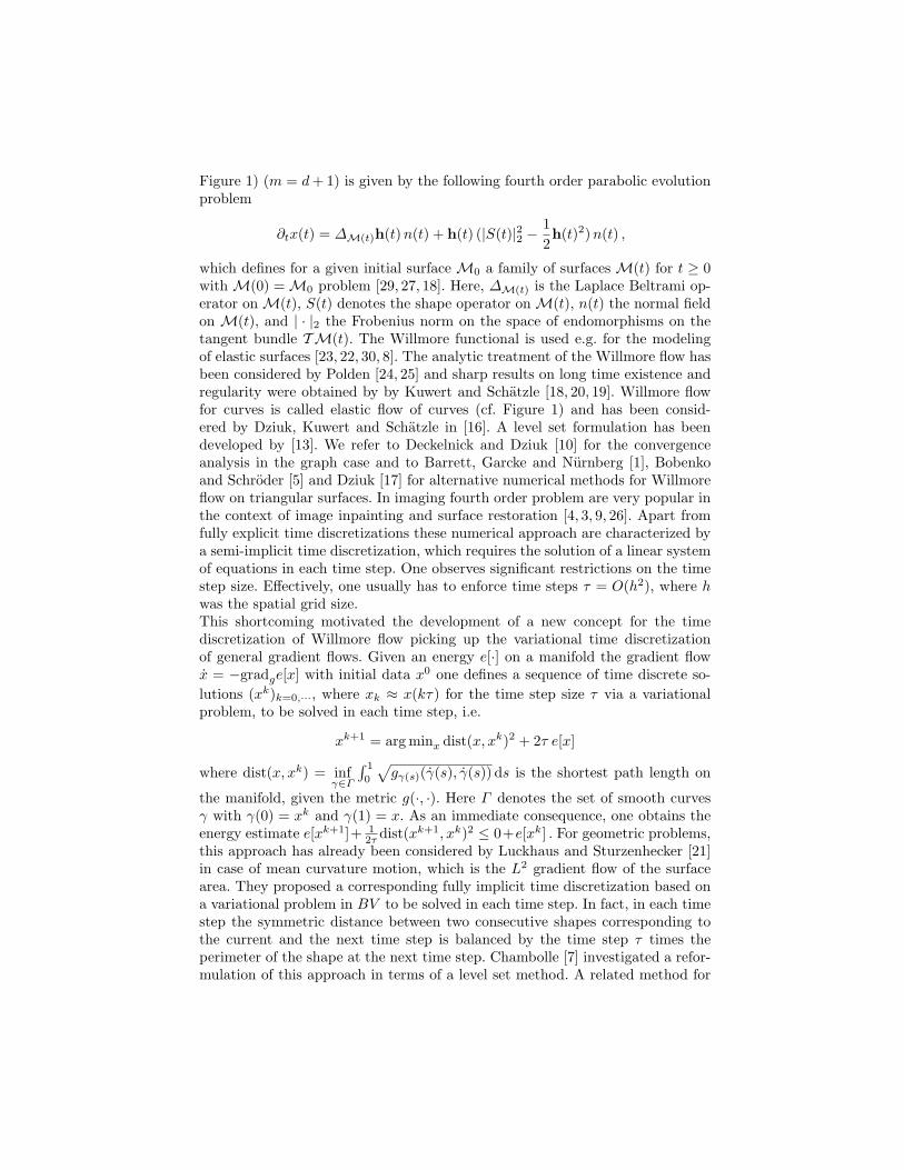
Figure 1) (m = d + 1) is given by the following fourth order parabolic evolutionproblem

∂tx(t) = ∆M(t)h(t) n(t) + h(t) (|S(t)|22 −12h(t)2) n(t) ,

which defines for a given initial surface M0 a family of surfaces M(t) for t ≥ 0with M(0) = M0 problem [29, 27, 18]. Here, ∆M(t) is the Laplace Beltrami op-erator on M(t), S(t) denotes the shape operator on M(t), n(t) the normal fieldon M(t), and | · |2 the Frobenius norm on the space of endomorphisms on thetangent bundle TM(t). The Willmore functional is used e.g. for the modelingof elastic surfaces [23, 22, 30, 8]. The analytic treatment of the Willmore flow hasbeen considered by Polden [24, 25] and sharp results on long time existence andregularity were obtained by by Kuwert and Schatzle [18, 20, 19]. Willmore flowfor curves is called elastic flow of curves (cf. Figure 1) and has been consid-ered by Dziuk, Kuwert and Schatzle in [16]. A level set formulation has beendeveloped by [13]. We refer to Deckelnick and Dziuk [10] for the convergenceanalysis in the graph case and to Barrett, Garcke and Nurnberg [1], Bobenkoand Schroder [5] and Dziuk [17] for alternative numerical methods for Willmoreflow on triangular surfaces. In imaging fourth order problem are very popular inthe context of image inpainting and surface restoration [4, 3, 9, 26]. Apart fromfully explicit time discretizations these numerical approach are characterized bya semi-implicit time discretization, which requires the solution of a linear systemof equations in each time step. One observes significant restrictions on the timestep size. Effectively, one usually has to enforce time steps τ = O(h2), where hwas the spatial grid size.This shortcoming motivated the development of a new concept for the timediscretization of Willmore flow picking up the variational time discretizationof general gradient flows. Given an energy e[·] on a manifold the gradient flowx = −gradge[x] with initial data x0 one defines a sequence of time discrete so-lutions (xk)k=0,···, where xk ≈ x(kτ) for the time step size τ via a variationalproblem, to be solved in each time step, i.e.

xk+1 = arg minx dist(x, xk)2 + 2τ e[x]

where dist(x, xk) = infγ∈Γ

∫ 1

0

√gγ(s)(γ(s), γ(s)) ds is the shortest path length on

the manifold, given the metric g(·, ·). Here Γ denotes the set of smooth curvesγ with γ(0) = xk and γ(1) = x. As an immediate consequence, one obtains theenergy estimate e[xk+1]+ 1

2τ dist(xk+1, xk)2 ≤ 0+e[xk] . For geometric problems,this approach has already been considered by Luckhaus and Sturzenhecker [21]in case of mean curvature motion, which is the L2 gradient flow of the surfacearea. They proposed a corresponding fully implicit time discretization based ona variational problem in BV to be solved in each time step. In fact, in each timestep the symmetric distance between two consecutive shapes corresponding tothe current and the next time step is balanced by the time step τ times theperimeter of the shape at the next time step. Chambolle [7] investigated a refor-mulation of this approach in terms of a level set method. A related method for

Fig. 1. Different time steps of the Willmore flow of an original ellipsoid curve with 100vertices is shown (top row). The time step size was chosen of the order of the spatialgrid size h = τ = 0.0632847. Willmore flow of a deformed sphere towards a roundsphere is depicted in the bottom row. We show the surface at times t = 0, t = τ ,t = 50τ , and t = 150τ , where τ = h = 0.02325548045.

anisotropic mean curvature motion is discussed in [2, 6].

In case of Willmore flow, we will proceed as follows. We aim at balancing thesquared distance of the unknown surface at time tk+1 = tk + τ from the currentsurface at time tk and a suitable approximation of the Willmore energy at timetk+1 scaled by twice the time step size. Solving a fully implicit time discreteproblem for mean curvature motion for the unknown surface at time tk+1, wecan regard the corresponding difference quotient in time as a time discrete,fully implicit approximation of the mean curvature vector. Based on this meancurvature vector, the Willmore functional can be approximated. Thus, we arelead to a nested minimization problem in each time step. In the inner problemon the new time step an implicit mean curvature vector is identified. Then, theouter problem is the actual implicit, variational formulation of Willmore flow.Indeed, the resulting two step time discretization experimentally turns out to beunconditionally stable and effectively allows for time steps of the order of thespatial grid size.

The paper is organized as follows. In Section 2 we derive the time discretescheme for Willmore flow, still continuous in space. Based on piecewise affinefinite elements on simplicial surfaces we derive a fully discrete numerical ap-proach in Section 3. In Section 4 the duality technique from PDE constraintoptimization is revisited to derive a minimization algorithm for the optimizationproblem. Finally, in Section 5 various examples for the Willmore of curves andsurfaces are investigated.

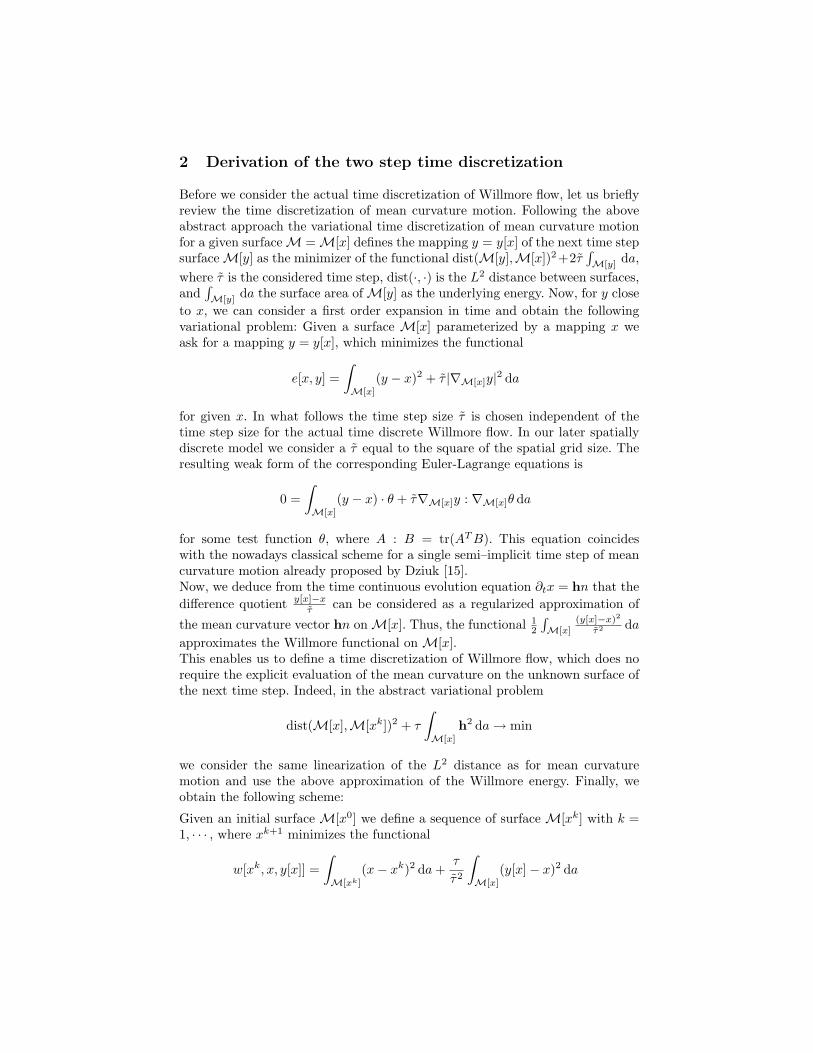
2 Derivation of the two step time discretization

Before we consider the actual time discretization of Willmore flow, let us brieflyreview the time discretization of mean curvature motion. Following the aboveabstract approach the variational time discretization of mean curvature motionfor a given surface M = M[x] defines the mapping y = y[x] of the next time stepsurface M[y] as the minimizer of the functional dist(M[y],M[x])2+2τ

∫M[y]

da,where τ is the considered time step, dist(·, ·) is the L2 distance between surfaces,and

∫M[y]

da the surface area of M[y] as the underlying energy. Now, for y closeto x, we can consider a first order expansion in time and obtain the followingvariational problem: Given a surface M[x] parameterized by a mapping x weask for a mapping y = y[x], which minimizes the functional

e[x, y] =∫M[x]

(y − x)2 + τ |∇M[x]y|2 da

for given x. In what follows the time step size τ is chosen independent of thetime step size for the actual time discrete Willmore flow. In our later spatiallydiscrete model we consider a τ equal to the square of the spatial grid size. Theresulting weak form of the corresponding Euler-Lagrange equations is

0 =∫M[x]

(y − x) · θ + τ∇M[x]y : ∇M[x]θ da

for some test function θ, where A : B = tr(AT B). This equation coincideswith the nowadays classical scheme for a single semi–implicit time step of meancurvature motion already proposed by Dziuk [15].Now, we deduce from the time continuous evolution equation ∂tx = hn that thedifference quotient y[x]−x

τ can be considered as a regularized approximation of

the mean curvature vector hn on M[x]. Thus, the functional 12

∫M[x]

(y[x]−x)2

τ2 da

approximates the Willmore functional on M[x].This enables us to define a time discretization of Willmore flow, which does norequire the explicit evaluation of the mean curvature on the unknown surface ofthe next time step. Indeed, in the abstract variational problem

dist(M[x],M[xk])2 + τ

∫M[x]

h2 da → min

we consider the same linearization of the L2 distance as for mean curvaturemotion and use the above approximation of the Willmore energy. Finally, weobtain the following scheme:

Given an initial surface M[x0] we define a sequence of surface M[xk] with k =1, · · · , where xk+1 minimizes the functional

w[xk, x, y[x]] =∫M[xk]

(x− xk)2 da +τ

τ2

∫M[x]

(y[x]− x)2 da

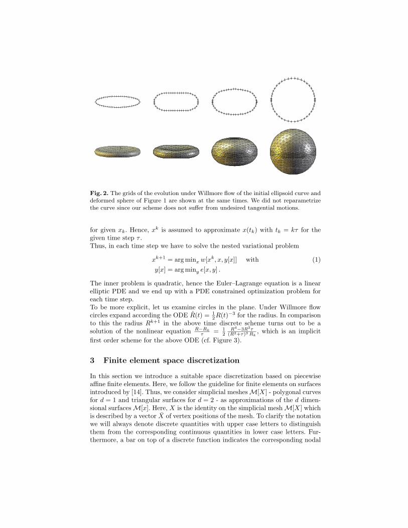
Fig. 2. The grids of the evolution under Willmore flow of the initial ellipsoid curve anddeformed sphere of Figure 1 are shown at the same times. We did not reparametrizethe curve since our scheme does not suffer from undesired tangential motions.

for given xk. Hence, xk is assumed to approximate x(tk) with tk = kτ for thegiven time step τ .Thus, in each time step we have to solve the nested variational problem

xk+1 = arg minx w[xk, x, y[x]] with (1)y[x] = arg miny e[x, y] .

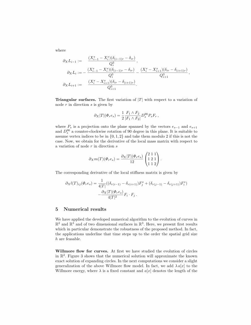
The inner problem is quadratic, hence the Euler–Lagrange equation is a linearelliptic PDE and we end up with a PDE constrained optimization problem foreach time step.To be more explicit, let us examine circles in the plane. Under Willmore flowcircles expand according the ODE R(t) = 1

2R(t)−3 for the radius. In comparisonto this the radius Rk+1 in the above time discrete scheme turns out to be asolution of the nonlinear equation R−Rk

τ = 12

R4−3R2τ(R2+τ)3 Rk

, which is an implicitfirst order scheme for the above ODE (cf. Figure 3).

3 Finite element space discretization

In this section we introduce a suitable space discretization based on piecewiseaffine finite elements. Here, we follow the guideline for finite elements on surfacesintroduced by [14]. Thus, we consider simplicial meshes M[X] - polygonal curvesfor d = 1 and triangular surfaces for d = 2 - as approximations of the d dimen-sional surfaces M[x]. Here, X is the identity on the simplicial mesh M[X] whichis described by a vector X of vertex positions of the mesh. To clarify the notationwe will always denote discrete quantities with upper case letters to distinguishthem from the corresponding continuous quantities in lower case letters. Fur-thermore, a bar on top of a discrete function indicates the corresponding nodal

vector, i.e. X = (Xi)i∈I , where Xi = (X1i , · · · , Xm

i ) is the coordinate vector ofthe ith vertex of the mesh and I denotes the index set of vertices.Hence, given some initial surface M[X0] we seek a sequence of discrete surfaces(M[Xk])k=1,··· of discrete surfaces. Locally, using also local indices each elementT of a polygonal curve is a line segment with nodes X1 and X2 and elementsT of a triangulation are planar triangles with vertices X0, X1, and X2 and facevectors F0 = X2 − X1, F1 = X0 − X2, and F2 = X1 − X0. Given a simplicialsurface M[X] we denote by

V(M[X]) :={U ∈ C0(M[X]) |Φ|T ∈ P1 ∀T ∈M[X]

}.

the corresponding piecewise affine Finite Element space consisting of those func-tions being affine on each element T of M[X]. With a slight misuse of no-tation the mapping X itself is considered as an element in V(M[X])m. Let{Φi}i∈I be the nodal basis of V(M[X]). Thus, for U ∈ V(M[X]) we obtainU =

∑i∈I U(Xi)Φi and U = (U(Xi))i∈I , in particular in accordance to our

above definition we recover X = (Xi)i∈I .Next, let us introduce the mass matrix M [X] and the stiffness matrix L[X] onthe discrete surface M[X], whose entries are given by

Mij [X] =∫M[X]

ΦiΦj da, Lij [X] =∫M[X]

∇M[X]Φi · ∇M[X]Φj da .

To apply mass and stiffness matrices to discrete maps from M[X] to Rm, weneed corresponding block matrices M[X] and L[X] in Rm]I×m]I :

M[X] =

M [X]M [X]

M [X]

, L[X] =

L[X]L[X]

L[X]

.

Both, mass and stiffness matrix M and L can be assembled from correspond-ing local mass and stiffness matrices m(T ) and l(T ) for all simplices T on M[X].

Now, we have all the ingredients at hand to derive the fully discrete two steptime discretization of Willmore flow (cf. Figure 2), which is can be regarded asdiscrete counterpart of (1). Given a discrete surface M(Xk) in time step k wedefine Xk+1 ∈ V(M[Xk])m as the minimizer of the following spatially discrete,nested variational problem

Xk+1 = arg minX∈V(M[Xk])m W [Xk, X, Y [X]] with (2)Y [X] = arg minY ∈V(M[X])m E[X, Y ] ,

where

E[X, Y ] :=∫M[X]

(Y −X)2 + τ |∇M[X]Y |2 da

= M[X](Y − X) · (Y − X) + τL[X]Y · Y ,

W [Xk, X, Y ] :=∫M[Xk]

(X −Xk)2 da +τ

τ2

∫M[X]

(Y −X)2 da

= M[Xk](X − Xk) · (X − Xk) +τ

τ2M[X](Y − X) · (Y − X)

are the straightforward spatially discrete counterpart of the functionals e[x, y]and w[xk, x, y], respectively. In analogy to the continuous case for given X thenodal vector Y [X] solves the a linear system of equation

(M[X] + τL[X]) Y [X] = M[X] X . (3)

For the sake of completeness let us finally give explicit formulas for the entriesof the mass and stiffness matrices. Later in Section 4 we will have to computevariations of these entries as well.

Polygonal curve. In the case of curves we consider a lumped mass matrix (cf.[28]) and obtain directly for the global matrices

M [X] = diag(

12(Qi + Qi+1)

), L[X] = tridiag

(− 1

Qi,

1Qi

+1

Qi+1,− 1

Qi+1

)where Qi = |Xi − Xi−1| is the length of the jth line segment and diag() andtridiag() denote diagonal or tridiagonal matrices with the corresponding entriesin each row. Here, we assume a cyclic indexing, i.e. we identify the indices i = 1and i = ]I + 1 for closed curves with X0 = X]I .

Triangular surfaces. Due to the greater variability of triangular surfaces com-pared to polygonal curves, let us consider the local matrices on triangles sepa-rately. Denoting the local basis function on a triangle T by Φ0, Φ1, Φ3, whereΦi(Xj) = δij (with δij being the usual Kronecker symbol) we verify by a simplestraightforward computation (cf. [12]) that

m(T ) =

∫T

ΦiΦj da

i,j=0,1,2

=|T |12

2 1 11 2 11 1 2

,

with |T | = 12 |F2 ∧ F1| being the area of the triangle T , and

l(T )ij =∫T

∇T Φi · ∇T Φj da =Fi · Fj

4|T |,

where ∇T the gradient on planar T .

4 Numerical solution of the optimization problem

In this section, we discuss how to numerically solve in each time step the non-linear optimization problem (2). Here, we will confine to a gradient descentapproach and take into account a suitable duality technique to effectively com-pute the gradient of the energy functional W [X] = W [Xk, X, Y [X]] given thefact that the argument Y [X] is a solution of the inner minimization problemand as such solves the linear system of equations (3). Indeed, we obtain for thevariation of W in a direction Θ ∈ V(M[Xk])m

∂XW [X](Θ) = ∂XW [Xk, X, Y [X]](Θ) + ∂Y W [Xk, X, Y [X]] (∂XY [X](Θ)) .

A direct computation of ∂XY [X](Θ) would require the solution of the innerminimization problem and thus specifically a linear system (cf. (3)) would haveto be solved for every test function Θ. This can be avoided applying the followingduality argument:

From the optimality of Y [X] in the inner problem, we deduce the equation0 = ∂Y E[Y [X], X](Ψ) for any test function Ψ ∈ V(M[X])m. Now, differentiatingwith respect to X we obtain

0 = ∂X (∂Y E[Y [X], X](Ψ)) (Θ)= ∂X∂Y E[Y, X](Ψ,Θ) + ∂2

Y E[Y [X], X](Ψ, ∂XY [X](Θ))

for any test function Ψ . Let us now define P ∈ V(M[Xk])m as the solution ofthe dual problem

∂2Y E[Y [X], X](P, Ψ) = ∂Y W [Xk, X, Y [X]](Ψ) . (4)

for all test functions Ψ ∈ V(M[Xk])m. Now, choosing Ψ = ∂XY [X](Θ) oneobtains

(∂Y W ) [Xk, X, Y [X]] (∂XY [X](Θ)) = −∂X∂Y E[Y, X](P,Θ) .

Thus, we can finally rewrite the variation of W with respect to X in a directionΘ as

∂XW [X](Θ) = ∂XW [Xk, X, Y [X]](Θ)− ∂X∂Y E[Y, X](P,Θ). (5)

The solution P of the dual problem (4) requires to solve∫M[X]

P · Ψ + τ∇M[X]P : ∇M[X]Ψ da =∫

M[X]

τ

τ2(Y −X) · Ψ da

for all test functions Ψ . In matrix vector notation, this can be written as thelinear system of equations

(M[X] + τL[X]) P =τ

τ2M[X](Y − X) .

The terms on the right hand side of (5) are to be evaluated as follows

(∂XW ) [Xk, X, Y ](Θ) = 2M[Xk](X − Xk) · Θ + 2τ

τ2M[X](X − Y ) · Θ

+τ

τ2(∂XM[X](Θ))(Y − X) · (Y − X) ,

∂X∂Y E[Y, X](P,Θ) = ∂X

(2M[X](Y − X) · P + 2τL[X]Y · P

)(Θ)

= 2(∂XM[X](Θ))(Y − X) · P − 2M[X]Θ · P

+2τ(∂XL[X](Θ))Y · P .

It remains to compute the variation of the mass and stiffness matrix with respectto a variation θ of the simplicial grid,

∂XM[X](Θ) =

∂XM [X](Θ)∂XM [X](Θ)

∂XM [X](Θ)

,

∂XL[X](Θ) =

∂XL[X](Θ)∂XL[X](Θ)

∂XL[X](Θ)

,

where ∂XM [X](Θ) = ddεM [X + ε Θ]|ε=0 and ∂XL[X](Θ) = d

dεL[X + ε Θ]|ε=0.Finally, we can compute the descent direction in Rm]I of the energy W at agiven simplicit mesh M[X] described by the nodal vector X and obtain

gradXW [X] =(∂XW [X](Φres)

)r∈I, s=1,··· ,m

,

where es denotes the sth coordinate direction in Rm.In the concrete numerical algorithm we now perform a gradient descent methodwith the Amijo step size control starting from the initial position given by theprevious time step.

Polygonal curve. We obtain for the derivatives of the mass matrix (usingagain the usual Kroneckersymbol δir) with respect to a variation of node r indirection s

∂XM [X](Φres) = diag(

(Xsi−1−Xs

i )(δ(i−1)r−δir)2Qi

+(Xs

i−Xsi+1)(δir−δ(i+1)r)2Qi+1

),

where as above Qi = |Xi−Xi−1|. Furthemore, we get for the derivatives for thestiffness matrix in the same direction

∂XL[X](Φres) = tridiag(∂XLi−1, ∂XLi, ∂XLi+1),

where

∂XLi−1 :=(Xs

i−1 −Xsi )(δ(i−1)r − δir)Q3

i

,

∂XLi :=−(Xs

i−1 −Xsi )(δ(i−1)r − δir)Q3

i

−(Xs

i −Xsi+1)(δir − δ(i+1)r)

Q3i+1

,

∂XLi+1 :=(Xs

i −Xsi+1)(δir − δ(i+1)r)

Q3i+1

.

Triangular surfaces. The first variation of |T | with respect to a variation ofnode r in direction s is given by

∂X |T |(Φres) =12

F1 ∧ F2

|F1 ∧ F2|D90

s PsFr ,

where Ps is a projection onto the plane spanned by the vectors es−1 and es+1

and D90s a counter-clockwise rotation of 90 degree in this plane. It is suitable to

assume vertex indices to be in {0, 1, 2} and take them modulo 2 if this is not thecase. Now, we obtain for the derivative of the local mass matrix with respect toa variation of node r in direction s

∂Xm(T )(Φres) =∂X |T |(Φres)

12

2 1 11 2 11 1 2

.

The corresponding derivative of the local stiffness matrix is given by

∂X l(T )ij(Φres) =1

4|T |((δr(i−1) − δr(i+1))F s

j + (δr(j−1) − δr(j+1))F si )

−∂X |T |(Φres)4|T |2

Fi · Fj .

5 Numerical results

We have applied the developed numerical algorithm to the evolution of curves inR2 and R3 and of two dimensional surfaces in R3. Here, we present first resultswhich in particular demonstrate the robustness of the proposed method. In fact,the applications underline that time steps up to the order the spatial grid sizeh are feasable.

Willmore flow for curves. At first we have studied the evolution of circlesin R2. Figure 3 shows that the numerical solution will approximate the knownexact solution of expanding circles. In the next computations we consider a slightgeneralization of the above Willmore flow model. In fact, we add λ a[x] to theWillmore energy, where λ is a fixed constant and a[x] denotes the length of the

4.1

4.0

3.9900 1000

4

3

20 200 400 600 800 1000

Fig. 3. A circle of radius R0 = 2 expands in two dimension due to its propagationvia Willmore flow (left)). The exact solution (grey dashed line) and the correspondingdiscrete solution computed by the two step time discretization for 200 polygon verticesand a time step size which equals the grid size (green crosses) are plotted for differenttimes t = 100 h, 500 h, 1000 h. The radius of the growing circle under Willmore flowis plotted for the known continuous solution (green) and the discrete solution (red).(right)

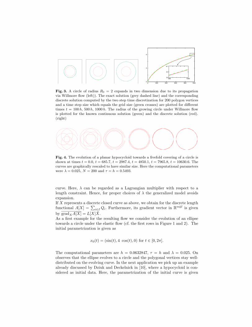
Fig. 4. The evolution of a planar hypocycloid towards a fivefold covering of a circle isshown at times t = 0.0, t = 685.7, t = 2987.4, t = 4850.1, t = 7965.8, t = 10630.6. Thecurves are graphically rescaled to have similar size. Here the computational parameterswere λ = 0.025, N = 200 and τ = h = 0.5493.

curve. Here, λ can be regarded as a Lagrangian multiplier with respect to alength constraint. Hence, for proper choices of λ the generalized model avoidsexpansion.If X represents a discrete closed curve as above, we obtain for the discrete lengthfunctional A[X] =

∑i∈I Qi. Furthermore, its gradient vector in Rm]I is given

by gradXA[X] = L[X]X.As a first example for the resulting flow we consider the evolution of an ellipsetowards a circle under the elastic flow (cf. the first rows in Figure 1 and 2). Theinitial parametrization is given as

x0(t) = (sin(t), 4 cos(t), 0) for t ∈ [0, 2π].

The computational parameters are h = 0.0632847, τ = h and λ = 0.025. Onobserves that the ellipse evolves to a circle and the polygonal vertices stay well-distributed on the evolving curve. In the next application we pick up an examplealready discussed by Dziuk and Deckelnick in [10], where a hypocycloid is con-sidered as initial data. Here, the parametrization of the initial curve is given

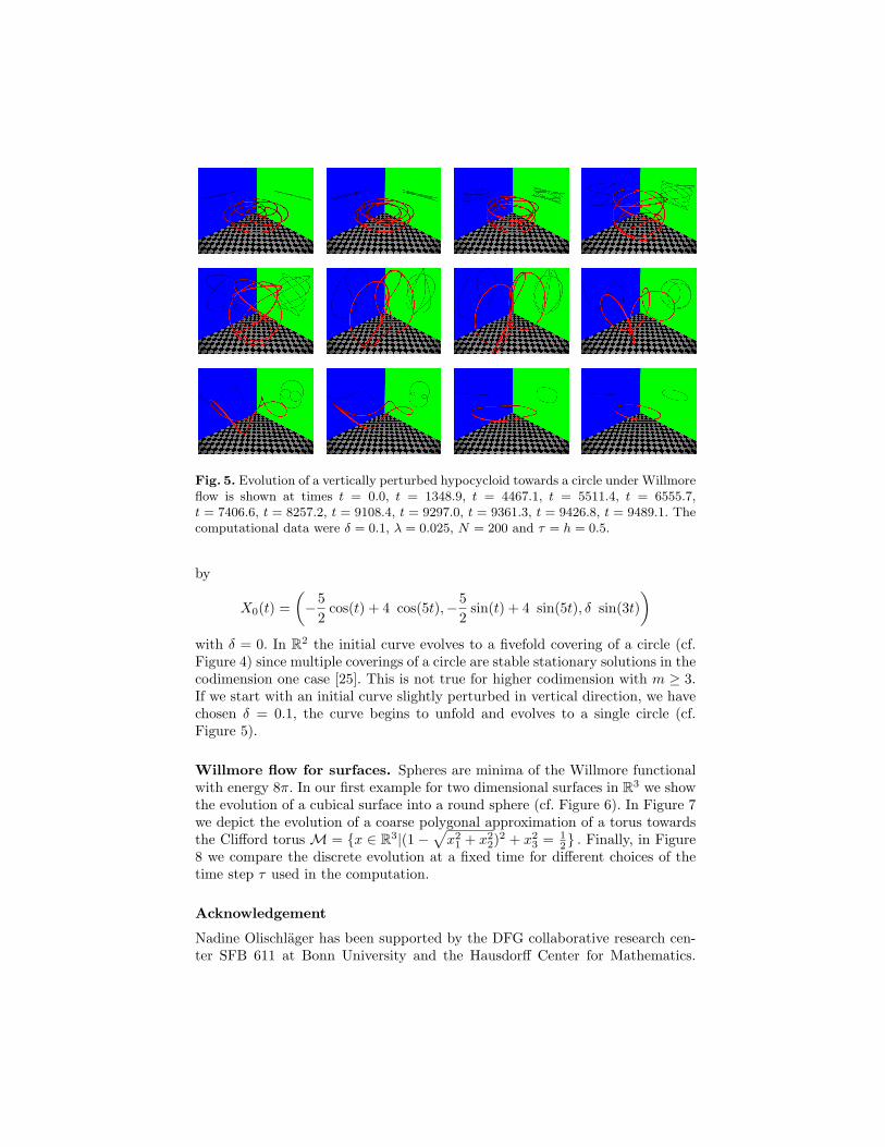
Fig. 5. Evolution of a vertically perturbed hypocycloid towards a circle under Willmoreflow is shown at times t = 0.0, t = 1348.9, t = 4467.1, t = 5511.4, t = 6555.7,t = 7406.6, t = 8257.2, t = 9108.4, t = 9297.0, t = 9361.3, t = 9426.8, t = 9489.1. Thecomputational data were δ = 0.1, λ = 0.025, N = 200 and τ = h = 0.5.

by

X0(t) =(−5

2cos(t) + 4 cos(5t),−5

2sin(t) + 4 sin(5t), δ sin(3t)

)with δ = 0. In R2 the initial curve evolves to a fivefold covering of a circle (cf.Figure 4) since multiple coverings of a circle are stable stationary solutions in thecodimension one case [25]. This is not true for higher codimension with m ≥ 3.If we start with an initial curve slightly perturbed in vertical direction, we havechosen δ = 0.1, the curve begins to unfold and evolves to a single circle (cf.Figure 5).

Willmore flow for surfaces. Spheres are minima of the Willmore functionalwith energy 8π. In our first example for two dimensional surfaces in R3 we showthe evolution of a cubical surface into a round sphere (cf. Figure 6). In Figure 7we depict the evolution of a coarse polygonal approximation of a torus towardsthe Clifford torus M = {x ∈ R3|(1−

√x2

1 + x22)

2 + x23 = 1

2} . Finally, in Figure8 we compare the discrete evolution at a fixed time for different choices of thetime step τ used in the computation.

Acknowledgement

Nadine Olischlager has been supported by the DFG collaborative research cen-ter SFB 611 at Bonn University and the Hausdorff Center for Mathematics.

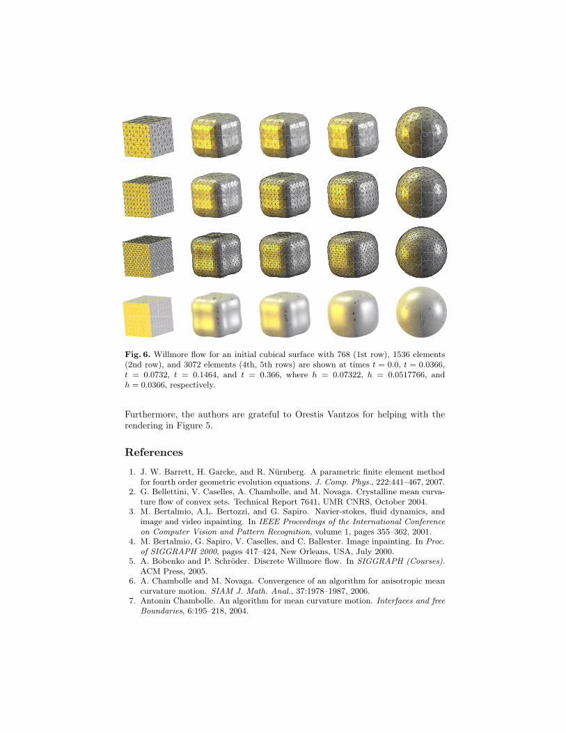
Fig. 6. Willmore flow for an initial cubical surface with 768 (1st row), 1536 elements(2nd row), and 3072 elements (4th, 5th rows) are shown at times t = 0.0, t = 0.0366,t = 0.0732, t = 0.1464, and t = 0.366, where h = 0.07322, h = 0.0517766, andh = 0.0366, respectively.

Furthermore, the authors are grateful to Orestis Vantzos for helping with therendering in Figure 5.

References

1. J. W. Barrett, H. Garcke, and R. Nurnberg. A parametric finite element methodfor fourth order geometric evolution equations. J. Comp. Phys., 222:441–467, 2007.

2. G. Bellettini, V. Caselles, A. Chambolle, and M. Novaga. Crystalline mean curva-ture flow of convex sets. Technical Report 7641, UMR CNRS, October 2004.

3. M. Bertalmio, A.L. Bertozzi, and G. Sapiro. Navier-stokes, fluid dynamics, andimage and video inpainting. In IEEE Proceedings of the International Conferenceon Computer Vision and Pattern Recognition, volume 1, pages 355–362, 2001.

4. M. Bertalmio, G. Sapiro, V. Caselles, and C. Ballester. Image inpainting. In Proc.of SIGGRAPH 2000, pages 417–424, New Orleans, USA, July 2000.

5. A. Bobenko and P. Schroder. Discrete Willmore flow. In SIGGRAPH (Courses).ACM Press, 2005.

6. A. Chambolle and M. Novaga. Convergence of an algorithm for anisotropic meancurvature motion. SIAM J. Math. Anal., 37:1978–1987, 2006.

7. Antonin Chambolle. An algorithm for mean curvature motion. Interfaces and freeBoundaries, 6:195–218, 2004.

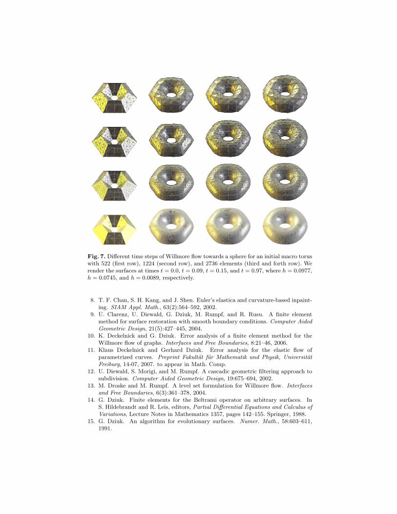
Fig. 7. Different time steps of Willmore flow towards a sphere for an initial macro toruswith 522 (first row), 1224 (second row), and 2736 elements (third and forth row). Werender the surfaces at times t = 0.0, t = 0.09, t = 0.15, and t = 0.97, where h = 0.0977,h = 0.0745, and h = 0.0089, respectively.

8. T. F. Chan, S. H. Kang, and J. Shen. Euler’s elastica and curvature-based inpaint-ing. SIAM Appl. Math., 63(2):564–592, 2002.

9. U. Clarenz, U. Diewald, G. Dziuk, M. Rumpf, and R. Rusu. A finite elementmethod for surface restoration with smooth boundary conditions. Computer AidedGeometric Design, 21(5):427–445, 2004.

10. K. Deckelnick and G. Dziuk. Error analysis of a finite element method for theWillmore flow of graphs. Interfaces and Free Boundaries, 8:21–46, 2006.

11. Klaus Deckelnick and Gerhard Dziuk. Error analysis for the elastic flow ofparametrized curves. Preprint Fakultat fur Mathematik und Physik, UniversitatFreiburg, 14-07, 2007. to appear in Math. Comp.

12. U. Diewald, S. Morigi, and M. Rumpf. A cascadic geometric filtering approach tosubdivision. Computer Aided Geometric Design, 19:675–694, 2002.

13. M. Droske and M. Rumpf. A level set formulation for Willmore flow. Interfacesand Free Boundaries, 6(3):361–378, 2004.

14. G. Dziuk. Finite elements for the Beltrami operator on arbitrary surfaces. InS. Hildebrandt and R. Leis, editors, Partial Differential Equations and Calculus ofVariations, Lecture Notes in Mathematics 1357, pages 142–155. Springer, 1988.

15. G. Dziuk. An algorithm for evolutionary surfaces. Numer. Math., 58:603–611,1991.

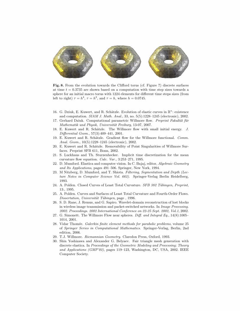
Fig. 8. From the evolution towards the Clifford torus (cf. Figure 7) discrete surfacesat time t = 0.3735 are shown based on a computation with time step sizes towards asphere for an initial macro torus with 1224 elements for different time steps sizes (fromleft to right) τ = h4, τ = h2, and τ = h, where h = 0.0745.

16. G. Dziuk, E. Kuwert, and R. Schatzle. Evolution of elastic curves in Rn: existenceand computation. SIAM J. Math. Anal., 33, no. 5(5):1228–1245 (electronic), 2002.

17. Gerhard Dziuk. Computational parametric Willmore flow. Preprint Fakultat furMathematik und Physik, Universitat Freiburg, 13-07, 2007.

18. E. Kuwert and R. Schatzle. The Willmore flow with small initial energy. J.Differential Geom., 57(3):409–441, 2001.

19. E. Kuwert and R. Schatzle. Gradient flow for the Willmore functional. Comm.Anal. Geom., 10(5):1228–1245 (electronic), 2002.

20. E. Kuwert and R. Schatzle. Removability of Point Singularities of Willmore Sur-faces. Preprint SFB 611, Bonn, 2002.

21. S. Luckhaus and Th. Sturzenhecker. Implicit time discretization for the meancurvature flow equation. Calc. Var., 3:253–271, 1995.

22. D. Mumford. Elastica and computer vision. In C. Bajaj, editor, Algebraic Geometryand Its Applications, pages 491–506. Springer, New York, 1994.

23. M Nitzberg, D. Mumford, and T. Shiota. Filtering, Segmentation and Depth (Lec-ture Notes in Computer Science Vol. 662). Springer-Verlag Berlin Heidelberg,1993.

24. A. Polden. Closed Curves of Least Total Curvature. SFB 382 Tubingen, Preprint,13:, 1995.

25. A. Polden. Curves and Surfaces of Least Total Curvature and Fourth-Order Flows.Dissertation, Universitat Tubingen, page , 1996.

26. S. D. Rane, J. Remus, and G. Sapiro. Wavelet-domain reconstruction of lost blocksin wireless image transmission and packet-switched networks. In Image Processing.2002. Proceedings. 2002 International Conference on 22-25 Sept. 2002, Vol.1, 2002.

27. G. Simonett. The Willmore Flow near spheres. Diff. and Integral Eq., 14(8):1005–1014, 2001.

28. Vidar Thomee. Galerkin finite element methods for parabolic problems, volume 25of Springer Series in Computational Mathematics. Springer-Verlag, Berlin, 2ndedition, 2006.

29. T.J. Willmore. Riemannian Geometry. Claredon Press, Oxford, 1993.30. Shin Yoshizawa and Alexander G. Belyaev. Fair triangle mesh generation with

discrete elastica. In Proceedings of the Geometric Modeling and Processing; Theoryand Applications (GMP’02), pages 119–123, Washington, DC, USA, 2002. IEEEComputer Society.