Two-Sided Markets in Asset Management: Exchange-traded Funds and Securities Lending

ABSTRACT

Asset management has long been a simple, fee-for-service business. Recently, however, exchange-traded funds have become increasingly engaged in two-sided markets between investors and stock borrowers. We show that fees from lending securities on average match expense ratios and, in many cases, can be much higher. We also test for two-sidedness by showing that the ratio of lending fees to expense ratio drives asset growth. Managers respond to these incentives by slanting their holdings toward stocks with higher lending fees. The results should be important for investors, who are no longer the customer buying service but are the product being sold.

Current version: December 5, 2015

1

Two-Sided Markets in Asset Management: Exchange-traded Funds and Securities Lending

“I would like to think the cost of investing [in ETFs] could come down to zero. There will always be a fixed cost in there, but if [a firm’s asset] volume is big [enough], the total expense ratio can come right down…in theory, we could pay investors to invest in us [as] stock lending can [create] a negative TER (total expense ratio).”

- Nick Blake, head of retail at Vanguard Investments, Vanguard raises the possibility of free ETFs, Financial Times, April 2, 2013

For decades, the asset management business has used a standard principal-agent model in

which investors pay managers for services rendered. Passive investment strategies in the form of

exchange-traded funds (ETF) and index mutual funds (IMF) fit into this framework, charging

much lower fees providing index returns. ETFs and IMFs have both grown in popularity, with

their combined AUM recently exceeding that of hedge funds1— $2.6 vs $2.1 trillion. For ETFs

and IMFs, the value proposition is clear: lower cost market or industry exposure. While this

suggests that passive investments are a low margin business, a recent Deutche Bank/McKinsey

study showed that ETFs are far more profitable than mutual funds.2 This high margin proposition

is consistent with the observed rapid growth of the ETF industry, whether measured in assets,

new ETF launches, or new ETF providers. Hence, we are faced with a puzzle. ETFs appear to be

structured like a commoditized, low margin business, but behave like an attractive, high-margin

business. Why?

In this study, we resolve this puzzle by showing that ETFs are following a fundamentally

different economic model: a two-sided market model of the type advanced by Rochet and Tirole

(2002), Parker and Van Alstyne (2005). In general, a two-sided market model is characterized by

a common platform that matches two sides of a transaction. A classic example is credit card

payment systems such as Visa/MasterCard. A credit card payment system matches customers

and vendors by providing a common transaction platform. The payment system may charge both

1 Mutual fund and exchange-traded fund data from the Investment Company Institute Factbook (2013), hedge fund data from BarclayHedge, accessed March 2014.

2 See “Low cost ETFs reap fat profits,” Financial Times, July 2011.

2

sides fixed or variable fees, which may even be negative (e.g. cash rewards credit cards with no

annual fee). More recent examples involve firms in the so-called “sharing economy” such as

Uber, and Airbnb. To be viable, each of these firms provides a common platform that must reach

critical mass on both sides to be viable. Indeed, this market model is so popular that a recent

Entrepreneur magazine article surveyed the plethora of new startups claiming to be the “Uber”

of various industries such as grocery delivery, laundry, medical marijuana, and lawn care.3

We propose that ETF industry’s rapid growth is a result of leveraging this same two-

sided market model. Each ETF is a platform to connect dispersed retail brokerage securities

holdings with institutional securities borrowers. The custodian cannot lend retail investors’ cash

brokerage account holdings without the prior consent of the account owner. Instead, each ETF

provides a standardized platform in the form of the ETF holdings specified by the index

benchmark. Retail investors may not have chosen exactly the same security portfolio, but, by

offering essentially the same overall expected return/risk profile at very low cost, ETFs facilitate

the standardization of retail holdings. The ETF, in turn, can then aggregate these holdings and

lend them at scale to larger, institutional clients who otherwise would not have access to those

dispersed assets.

As evidence that ETFs are using this innovative model, we show two primary results. The

First, and foremost, we document that revenue from securities lending is significant. ETFs are

making between 23-28 bps per year on average, compared to an average expense ratio of 26 bps.

If optimized, securities lending revenue can be as high as 55 to 114 bps per year. To illustrate

that this is a mainstream effect, not isolated to small and illiquid stocks, consider Figure 1. It

contains the weighted average lending fees of the stocks in the S&P 500 over time. Not

surprisingly, the figure shows a spike around the Financial Crisis of October 2008. At that time,

a broad array of securities including stocks became hard to borrow. During the past five years,

the value-weighted average lending fee has been about 40 bps per year. During the same interval,

the equal-weighted average rises to almost 60 bps before returning to about 40 bps. Contrast that

with the expense ratio of the primary S&P500 ETFs (IVV, VOO, SPY), which range from 5 to 7

3 We’re the Uber of X!, Entrepreneur, August 12, 2014 http://www.entrepreneur.com/article/236456

3

bps per year. While there are expenses associated with lending, even 20 bps of lending profit

dwarfs the 5 to 7 bps made charging investors.

Our second primary result implements the Rochet and Tirole identification test of two-

sided markets. Specifically, to be a two-sided market, the ratio of fees between the two sides, not

the overall level, must drive volume on the platform. To examine whether this is the case, we

compare the three biggest ETF providers: Blackrock (iShares), State Street Global Advisors

(SSgA), and Vanguard. These three providers account for about 90% of the total assets in our

ETF sample (i.e., U.S. domestic, physically replicated, equity ETFs). It would be preferable to

generate a matched sample of ETFs who are tracking the same index but have different expense

ratios and lending rates. This matched sample is ultimately identical to our test, however,

because the matching process identifies one ETF from each of the three for comparison. Smaller

competitors focus on niche products that rarely compete with these three larger market

participants, and these three larger companies compete in most areas.

In this three-firm analysis, we find that Vanguard is keeping more securities lending

revenue and charging lower expense ratios when compared with either SSgA or iShares. This

different ratio between lending revenues and expense ratio seems to be paying off with an

average asset growth rate more than double the other two. Historically, Vanguard was a

relatively late entrant to the ETF space, but has since grown so quickly that they are now the

second largest provider in this market. Thus it is possible that there are other, unobserved

differences that drive this growth, but it is not first- or even second-mover advantage. Overall,

we conclude that Vanguard’s different mix of fees is driving its large abnormal growth and that

ETFs are operating in a two-sided market.4

Active management, in contrast, is a one-sided market; two-sided markets are

fundamentally grounded in network effects and have increasing returns to scale. Actively

managed funds, however, have decreasing returns to scale (Pastor, Stambaugh, and Taylor

(2015), Chen et al. (2004)). Second, the management fees charged by active funds dwarf

4 A few large firms dominating a market like this is a common feature of two-sided markets. Consider Visa/MasterCard and American Express in payment systems and Xbox, Playstation, and Nintendo in game consoles, both of which are classic two-sided markets identified by Rochet and Tirole (2002).

4

securities lending revenue. Indeed, the most profitable stocks to lend have negative expected

returns since those high lending fees are driven by short selling demand. With mutual fund data,

Evans, Ferreira, and Prado (2015) have shown that selling those high-fee holdings is more

profitable than holding and lending.

In this paper, we focus on ETFs, although it may also be possible that passive index

mutual funds (IMFs) are following a two-sided market model. Unlike ETFs, IMFs have

increasing transaction costs with scale, and consequently do not enjoy the same network effects

as ETFs. Hence, we do not expect the results to as strong. We provide a matched-sample

comparison of ETFs vs IMFs and find that IMFs do not seem to generate securities lending

revenue at the same rate as corresponding ETFs. Higher transaction costs combined with lower

securities lending revenue implies that a two-sided market model is less lucrative for IMFs.

Indeed, they may not follow it at all.

Additional evidence that ETFs function as two-sided markets is the opening quote of the

paper, where a market participant suggests zero or negative expense ratios. Parker and Van

Alstyne (2005) apply a two-sided market framework to software that is given away in perpetuity.

A one-sided market cannot exist while giving the product away for free in perpetuity. In order

for this strategy to work, the zero (or negative) fee must be driving volume to the platform which

increases the net gains from trade among the matched parties and enables the platform provided

to generate profit by taking a portion of those gains from trade. While no exchange-traded funds

yet offer zero or negative expense ratios, the fact that industry participants believe them to be

possible in the near future gives insight into the underlying business model already in place.

This innovation in asset management has significant implications for academics,

practitioners, and retail investors. For academics, it is clear that exchange-traded funds do not

simply lie on one end of the continuum of delegated portfolio management. Principal-agent

models do not apply. Instead, new models incorporating the dual incentives of passive managers

(or management companies) need to be developed to better understand this market (e.g., Rochet

and Tirole 2006). We begin this process by providing evidence that ETF managers do, in fact,

slant their holdings toward securities that are more profitable to lend, that is, they respond to

their incentives. This behavior does not fit in a traditional principal-agent framework unless

security borrowers can be cast as the agents, an unlikely proposition.

5

For practitioners, two-sided markets can be very disruptive to the status quo. A decade

ago, Blackrock, State Street, and Vanguard were not primary players in the asset management

space. Now, they are seen as systemically important financial institutions (SIFI).5 Similarly,

Uber and Airbnb are disrupting the taxi and hotel businesses, respectively. A key message of our

paper to market practitioners is that ETFs in particular are not likely a fad and may be even more

of a threat to other asset managers than they are already.

Finally, ETF investors need to understand exactly what they are purchasing when they

buy an ETF. Investors in very low cost ETFs are not the customers, they are the product.

Investors provide the assets, which, in turn, are profitably lent out to generate revenue for the

fund provider. While novel in the financial sector, most consumers interact with this kind of

model every day when using Google, Facebook or the Wall Street Journal. This paper is, to the

best of our knowledge, the first to identify this model in the asset management business.

Our primary recommendation is for more transparency in this practice so ETF investors

can make an informed choice about what type of investment they want. We recommend that all

securities lending revenues, expenses, collateral, and counterparties be disclosed on audited

financial statements of the fund, along with the corresponding fees (to agent lenders, fund

provider, etc.). This disclosure would allow a transparent computation of securities lending

income shared with investors and risk assessment of collateral and counterparties. Some

investors may want a low (or zero, or negative) fee fund that surrenders all securities lending

income to the ETF provider. Another investor may prefer to pay a fixed annual fee in exchange

for a larger share in the more risky but potentially more profitable securities lending revenue.

These products could exist side by side in the marketplace and may even provide slightly

different risk-return profiles. Currently, even well informed investors cannot distinguish between

those fund structures.

The outline of the paper is as follows. The first section contains a brief review of the

relevant background literature and the second describes two-sided markets and their application

to exchange-traded funds in detail. The third contains descriptions of (a) the data sources, (b) the

5 Ultimately, they were not classified as such. See “Fund managers escape ‘systemic’ label,” Financial Times, July 14, 2015. http://www.ft.com/cms/s/0/4e9d566e-2999-11e5-8613-e7aedbb7bdb7.html

6

lending revenue estimation methodology, and (c) a summary of the attributes of our sample. In

section four, we focus on the estimates of securities lending revenue, and, in section five, we

discuss our tests on two-sided markets. Section six summarizes the conclusions of the study.

I. Background literature

The academic literature has little stand-alone research on passive investing, although

several unpublished papers on exchange-traded funds have appeared recently. The closest in

spirit to our work is Cheng, Massa, and Zhang (2015). They find that ETFs engage in cross-

subsidization and cross-trading within fund families increase fund revenues. Their sample and

purpose are distinctly different from ours, however. First, they use non-U.S. stocks. Our focus is

exclusively on U.S. stocks. Second, they focus on synthetic ETFs. Synthetic ETFs use swaps to

replicate index returns. Hence, their paper focuses primarily on the management of collateral.

We investigate traditional ETFs that hold portfolios of stocks and the revenues the stocks provide

from securities lending. Most of the remaining ETF literature focuses on the effect that ETFs

have on the underlying stocks. Ben-David, Franzoni, and Moussawi (2014), for example, show

that ETFs increase the return volatility of the underlying index. Da and Shive (2013) show that

ETFs increase the pairwise correlations among the returns of the stocks held in the ETF

portfolio.

The literature on securities lending is more developed. D'Avolio (2002) and Geczy,

Musto, and Reed (2002) introduce the equity lending market and provide the first empirical look

at how it functions, pricing, supply, and demand. Duffie, Garleanu, and Pedersen (2002) model

the market theoretically to incorporate search costs and show how the stock price can exceed

fundamental value since the stock price incorporates the expected revenue from lending. From

there, the research moved to investigating supply and demand shifts, first with data from a single

lender (Cohen, Diether, and Malloy (2007)), and more recently a broader study using data from

multiple lenders (Kolasinski, Reed, and Ringgenberg (2013)). Blocher, Reed, and Van Wesep

(2013) synthesize this literature in a simple supply and demand framework, linking the stock

market and lending market in joint equilibrium where prices are set simultaneously in both

markets. All of these studies either look at the market as a whole or from the demand side (i.e.,

primarily short sellers). Our study, on the other hand, focuses on the supply side of the equity

lending market.

7

To date, only two studies have focused on the supply side. Kaplan, Moskowitz, and

Sensoy (2013) engineer ‘shocks’ to the securities lending supply by convincing an active mutual

fund provider to make available some valuable stocks to lend and find little evidence of a stock

price effect. In a much more comprehensive investigation, Evans, Ferreira, and Prado (2015)

look at trends among active mutual funds and lending behavior, and its relation to the fund’s

overall performance and find several important stylized facts. First, during the period 1996

through 2008, they find that funds that lend securities underperform otherwise similar funds in

spite of lending income. Second, although 85% of the funds in their sample can lend, only 42%

actually do. Finally, the willingness to lend securities increased dramatically over their sample

period, from 15% of active funds in 1996 to 43% in 2008. While interesting in their own right,

neither of these studies addresses the issue of the profitability of securities lending behavior from

the perspective of passive funds.

II. Two-sided markets

The purpose of this section is to describe two-sided markets and how they relate to

exchange-traded funds. We draw on the work of Rochet and Tirole (2006), who summarize the

literature on two-sided markets and provide a model and a test for it presence. We begin by

describing some necessary (but not sufficient) features of two-sided markets and discuss how

they manifest themselves in exchange-traded funds. We then focus on Rochet and Tirole

(2006)’s necessary and sufficient condition for a two-sided market to exist.

One necessary condition for a two-sided market is increasing returns to scale. In Katz and

Shapiro (1985,1986), this arises from positive network externalities. In the active asset

management literature, however, consensus seems to be decreasing returns to scale. Pastor and

Stambaugh (2012) model decreasing returns to scale industry-wide. Empirical work by Pastor,

Stambaugh, and Taylor (2015) confirms this view. Berk and Green (2004) model decreasing

returns to scale at the individual fund level Empirical work by Chen et al. (2004) confirms this

view. In at least two ways, the sources of decreasing returns to scale for active managers are

obvious. First, greater size means greater transaction costs from price impact. Second, greater

size means greater demands on fund managers to identify profitable trades generating positive

and sustained alpha. These decreasing returns to scale or negative network externalities indicate

8

that active asset management does not (and, perhaps, even cannot) use the two-sided market

model.6

ETFs are different, however. First, greater scale for ETFs means greater liquidity and

lower transaction costs. In Table I, we report average daily dollar trading volume and average

relative spread for all ETFs listed in the monthly CRSP file by size decile. Note that average

daily trading volume and relative bid/ask spread are monotonically ordered with larger ETFs

displaying greater liquidity and lower spreads. Second, greater scale among ETFs means a more

effective arbitrage mechanism in the creation/redemption process.7 Third, since ETFs only

deliver index returns or beta, there is no problem with deploying capital at scale to generate

alpha. The primary challenge of large-scale index trackers is handling the less liquid index

constituents to minimize tracking error. Thus, ETFs exhibit positive network externalities

(positive returns to scale), consistent with two-sided markets.

A second necessary condition for a two-sided market is a platform that attracts both sides, in

contrast with intermediaries or aggregators who simply buy products for less than they sell. We

propose that each ETF is a platform. Retail investors, whose security holdings are not available

for lending8, sell disparate holdings and instead purchase an ETF that gives them a similar

expected return/risk profile. The lower cost of the ETF arises from fewer transactions and better

liquidity. In addition, securities lending revenue is now possible. This substitution effect is

illustrated in Figure 2, which shows the growth of ETF holdings by retail investors. Figure 2

shows three trends. The red line shows the rapid rise of retail holdings through ETFs. These data

are calculated by computing the retail holding % of ETFs and then multiplying that percentage

with the ETFs underlying holdings and then aggregating the shares held across all ETFs. We

then divide by shares outstanding to compute a % retail ownership passed through via retail ETF

holdings. The ratio has risen steeply from approximately 0% in 2000 to almost 5% of shares

6 Blocher (2015) finds positive network externalities among interconnected mutual fund flows, but they are short-term and non-fundamental (i.e. they reverse) and thus do not apply here.

7 For more on the ETF creation/redemption mechanism as well as ETF liquidity, see the ETF.com guide to ETFs at http://www.etf.com/etf-education-ce.html

8 Code of Federal Register 204.15c2-1. Margin accounts do allow the custodian to lend the securities, but these arrangements are rare among retail investors.

9

outstanding in 2013. The blue and green lines complement this trend, showing overall

institutional ownership (in blue) and institutional ownership less the retail holdings via ETFs as

computed above. The green (adjusted) line indicates a slight downward trend in institutional

ownership since 2008 indicating increased retail holdings, but mostly due to ‘pass-through’ retail

holdings via ETFs.

Once retail investors standardize on an ETF, then the ETF can lend securities on their

behalf at scale. There is some evidence that scale is important in securities lending. Hu, Pan, and

Wang (2015), for example, shows that aggregating assets is powerful strategy in repo markets.

Using the new N-MFP forms required since 2010 by the SEC for money market funds, Hu et al

provide two important inferences about tri-party repo transactions. First, they find that Fidelity

has a dominant position in equity repo transactions, and can demand better pricing for its repo

loans. Second, they find that relationships matter more than pricing since many dealers seem to

give the same proportion of business to all lenders (i.e., not ordering on price). Thus, we suggest

that as some ETF asset owners come to play prominent roles in the marketplace, they likely

achieve some manner of marginal pricing power.9

Institutional borrowers also prefer large quantities of passively held securities due to

recall risk (Engelberg, Reed, and Ringgenberg 2013). While most securities lending contracts are

overnight, in practice loans are perpetual until recalled by the lender or terminated by the

borrower. A primary reason for loan recall is the sale of the security by the beneficial owner.

Passively held assets have low turnover and predictable sales patterns based on index

performance. Thus, as the ETF grows in scale (assets), its lendable assets increase in value to

potential borrowers due to lower recall risk.

A final necessary, but not sufficient, condition for ETFs to be engaging in a two-sided

market is that lending fees must be substantial, that is, at least comparable to the expense ratios.

This is likely possible for passive fund managers (like ETFs) but not active fund managers.

Active managers, even of very large fund families, cannot significantly reduce their management

fees, increase their securities lending income, and increase market share. Management fees for

9 Market power is not a necessary condition of two-sided markets, but its presence makes two-sided markets more lucrative, as it does with one-sided markets.

10

active managers derive from transaction costs and compensation for skill. Higher transaction

costs result from higher turnover portfolio and higher compensation costs are required to

maintain skilled management teams focused on portfolio management. Securities lending

revenue, while possible, is a minor afterthought (if considered at all). We corroborate active

manager’s lack of interest in securities lending via anecdotal discussions with market

participants.10

Instead, a savvy active manager is likely to include any securities lending revenue into

fund alpha, which due to the flow-performance relation, will drive higher inflows, and positive

performance rather than using it to create a minor fee discount. No active manager can generate

significant alpha via securities lending because the most lucrative to lend (hard to borrow) have,

on average, negative expected returns (Blocher, Reed, and Van Wesep 2013) and thus should be

shorted or at least sold (Evans, Ferreira, and Prado 2015).

The market features discussed thus far, while satisfying necessary conditions for a two-

sided market, are not sufficient conditions. Rochet and Tirole (2006), however, provide a model

of two-sided markets in which both sides of the market are charged both fixed and variable rates

and the rates may be positive or negative. They show that a sufficient condition for a market to

be two-sided is that the split, or ratio, between fees drives volume to the common platform. This

is in contrast to the overall level of fees driving volume. If the overall level of fees is the driver

of volume, then this is still a traditional market with a low-cost provider. If the level of fees is

held constant and a shift in the ratio of fees drives volume, however, you have a two-sided

market. In the remainder of our study, we investigate whether the magnitude of lending fees or

the ratio of fees drive volume.

III. Data, lending revenue rate estimation, and sample description

The sample period of this study is January 2009 through December 2013. The data come

from a variety of sources. The first primary source of data is ETF holdings data from

Morningstar. These data include detailed holdings for all U.S.-based ETFs and are free of

10 We also note that Kaplan, Moskowitz, and Sensoy (2013) had to convince their active manager to begin lending shares to generate a supply shock, not vice versa.

11

survivorship bias.11 The sample period begins in 2009 because most ETFs began reporting daily

holdings around that time. From the universe of ETFs, we focus only on those that are physically

replicated using U.S. stocks. Funds that are replicated synthetically are not included. Also

excluded from the sample are inverse, leveraged, and preferred stock ETFs. Since Morningstar

does not include fields identifying these types of funds, they were identified by hand using fund

names. We also remove Unit Investment Trusts (UITs) because UITs are not allowed by statute

to lend securities. UITs include four well-known ETFs (SPY, QQQ, MDY, and DIA) as well as

Merrill Lynch’s now defunct HOLDRS line of ETFs.12 Finally, we remove obvious data errors

(e.g., funds that report holdings after their closing date or that report no asset value). Aside from

identifying fund holdings, the Morningstar data are also used to identify sectors, styles, and

equity-based strategies using the fund’s Category field.13

A second source is the ETF Classification System (ECS) data. The ECS data are from

ETF.com obtained on April 18, 2013 and contain most of the data from each ETF’s Prospectus

and Statement of Additional Information (SAI). This data set parses those regulatory documents

into 64 fields, including information about the index each ETF tracks, how the index is computed

(if known), and whether the fund is active (as defined by filings with the Securities and

Exchange Commission). This dataset also contains a Region field, with which we apply a

geographic filter. We keep funds whose region is North America, Global, Developed World, or

blank, all of which hold U.S. stocks. We exclude funds that are identified as active. Other fields

that we use from the ETF.com dataset include a flag for Proprietary Index (i.e., an indicator that

the ETF uses its own proprietary index methodology) and the expense ratio as calculated in the

annual report. The ETF holdings data from Morningstar are matched with the ECS data using

11 Most physically replicated ETFs (~99%) are governed by the Investment Company Act of 1940 and so have semi-annual reporting requirements like mutual funds. Because of the nature of ETFs creation/redemption mechanism, ETFs have a market-based incentive to publicly disclose highly accurate, detailed portfolios daily. These data are not typically archived by the ETFs. Morningstar, however, collects and stores the information and sells it.

12 Van Eck converted six of the HOLDRS funds into 1940 Act ETFs. These are included in our sample. (http://www.etf.com/sections/features/10553-all-the-holdrs-are-now-history-nyse-says.html) This action is consistent with our main thesis since UITs cannot lend securities, but 1940 Act funds can.

13 Sectors: Communications, Consumer Cyclical, Consumer Defensive, Equity Energy, Equity Precious Metals, Financial, Health, Industrials, Natural Resources, Real Estate, Technology, Utilities, and Miscellaneous. Styles: Small, Mid, Large intersected with Growth, Blend and Value (9 total).

12

ticker symbols. Note that the ETF.com dataset is a point-in-time snapshot, not a time series of

observations. For persistent variables like Region or Proprietary Index, the issue is of small

concern. But, since expense ratios have been trending downward, the use of data from the fund’s

latest reporting before or on April 13, 2013, may tend to understate expense ratios in the earlier

part of sample period. Spot checking annual reports from early in the sample period and

comparing them to the ETF.com levels suggests that the degree of bias is small.

Our final sample includes 541 unique ETFs. While this sample represents 26% of the

$2.6T in global ETF assets held at the end of 2013, it represents the whole population of

physically-replicated, US Equity ETFs, so there is no selection bias. For each ETF, we have total

net assets, number of holdings, and several asset allocation fields (% equities, sector allocations,

etc.). For each security held by an ETF, we have number of shares held, market value of those

shares, portfolio weight, currency, and type code (a detailed classification of security types). The

securities held are uniquely identified by CUSIP. Summary statistics for our sample of ETFs are

contained in Table II. Note that we have only 22,382 ETF-month observations, significantly

fewer than 32,460 total possible observations (541 ETFs times 60 months). This is because our

sample includes many new ETF launches as well as closures. While the mode of monthly

observations per fund is 60, the mean is 41 and the median is 51. Total Net Asset (TNA) values

are highly skewed. The mean is $866M, and the median is $107M. The minimum TNA of $0.6M

arises for funds just starting or about to close. The mean expense ratio is 47 bps, with a minimum

of 7 bps and maximum of 87 bps, all of which are as expected for physically replicated, passive

ETFs. The value-weighted expense ratio (not tabulated) is 26 bps, which indicates that larger

funds generally have lower expense ratios. The number of holdings range from 13 securities

(typical of a small sector fund) up to well over 3,500 securities, typical of a broad-based, ‘total-

market’ index ETF.14

Our holdings data on passive index mutual funds (IMFs) are from the Thomson Reuters

Mutual Fund Ownership files (formerly s12 data). These data are merged with the CRSP daily

stock data using MFLINKS. We use the CRSP index flag to identify index funds, remove ETFs

14 Note that TNA for ETFs has been adjusted for all Vanguard funds. See Appendix A for more information.

13

based on the ETF flag, and choose only equity mutual funds based on the CRSP objective code

(the first two digits of the code must be “ED”). Unfortunately, the MFLINKS data are only

updated through March 2012 so our sample of mutual funds ends there. It includes 173 mutual

funds, quarterly. The summary statistics are consistent with the stylized facts we know about

mutual funds versus ETFs. There are fewer IMFs, but with more assets, typically because of their

association with retirement plans. The mean TNA is $4.1B, median is $475M, both significantly

higher than the corresponding ETF measures. The expense ratios show more spread, ranging

from 2 bps to 245 bps and a standard deviation of 57 bps (versus 19 bps for ETFs).

Our securities lending data are from Markit (formerly Data Explorers). Markit collects

data from securities lending agents each day. The data coverage is quite large, accounting for

about 80% of U.S. equities. The file contains a number of fields for each “stock-day” (i.e., each

stock each day). One of the fields that we use in our analysis is the utilization ratio. The

utilization ratio equals the number of shares demanded divided by the number of shares supplied,

and measures how constrained the lending market is at any point in time. A utilization ratio of

one, for example, means that all available shares are lent out.

The Markit dataset also contains two important borrowing cost variables. The first is

indicative lending fees. Our analysis requires that we have a lending fee for each stock each day.

Unfortunately, these indicative fees will not serve the purpose since the data histories are

incomplete. The second borrowing cost variable is the Daily Cost to Borrow Score (DCBS). The

DCBS is a 1-10 integer categorization that describes how expensive a stock is to borrow, with 1

being the cheapest and 10 being the most expensive. The scores are computed by Markit for each

stock-day and are based on actual lending fees that they receive from securities dealers but are

not allowed to re-distribute.

To estimate lending fees for each stock-day, we devise a compromise methodology. First,

we gather all DCBS stock-day observations from the Markit data base. Occasionally, there are

multiple observations because the same stock can be reported on the same day. In these

instances, we round the average DCBS across duplicates to assign the nearest integer value.

Next, we take observations with lending fees and DCBS scores and assemble a distribution of

lending fees for the stocks in each DCBS category each month. Across all days in the sample

period, the mean (median) of the ratio of the number of lending fees to number of DCB Scores

14

was 53.8% (57.4%), ranging from a minimum of 24.3% to a maximum of 71.6%. From the

lending fee distribution each month, we compute (a) the mean, (b) the median, (c) the 5th

percentile (the “Low”), and (d) 95th percentile (the “High”) lending fees. The mean and the

median rates reflect the “typical” lending fee for stocks in each DCBS category each month. The

Low and the High reflect low-end and high-end estimates, while simultaneously mitigating the

effect of outliers. The four lending fee parameters are recorded for all stocks in each DCBS

category in each day during the month. Note that this is not to say that there is no variation in a

stock’s lending rate during the days of the month. There are many instances in which a stock’s

DCBS changes from day to day depending on the supply and demand to borrow. In our sample,

18.8% stocks changed DCBS categories between one and five times during a month, and 4.8% of

stocks changed categories six or more times.

Our lending fee estimation methodology also circumvents another problem associated

with the reported fees appearing in the Markit file, that is, noise. Since there is no standard

procedure in recording the fees each day, they can vary from day to day as a result of receiving

quotes from different dealers with different inventories. This noise makes reliable inferences

about the character of the market more challenging. Table III compares the raw lending fees with

the mean and median estimates from our methodology when both are available. The total number

of observations is 2,753,489. The mean reported lending fee is 113.36 bps. The estimated mean

and median fees are 120.96 bps and 103.31 bps, respectively. While the differences are

significant in a statistical sense, they are not economically meaningful at –7.60 bps and 10.05

bps, respectively. The standard deviation and range of the reported fees is the case in point,

however. For the reported fees, the standard deviation is 486.52 bps, with a range of –50.00 to

72,183.39 bps. The standard deviations of the mean and median fees, on the other hand, are

much smaller. Indeed, tests of the equivalence of the variances reject the hypotheses that the

variances of the estimated fees and the variance of the reported fees are the same. In other words,

our estimation methodology serves to reduce the variability in the lending fees by almost 10%

for the mean estimate and 20% for the median estimate.

Our primary source of stock market data is the daily CRSP file. From this file, we extract

closing share price, share return, shares outstanding, trading volume, and closing bid/ask price

quotes for each stock-day. These attributes allow us to develop an intuition for the association

between lending fees and the properties of the stocks within each DCBS category. In all, we have

15

lending fee and stock information for 5,066,530 unique stock-days from 6,329 different stocks

and 1,258 trading days in the sample period January 2009 through December 2013. Table IV

summarizes selected attributes of the stocks in the sample including the average market

capitalization (in millions of dollars), the average dollar trading volume (in millions of dollars),

the average relative trading volume (i.e., shares traded divided by shares outstanding), the

average annualized return volatility, the average relative bid/ask spread (i.e., the difference

between the ask price and the bid price divided by the bid/ask midpoint), as well as the mean and

median lending fees.

The results reported in Table IV are interesting and intuitive in a number of ways. First,

Category 1 stocks have incredibly high market capitalization—$4,852 million on average. This

stands to reason. Stocks with such a large presence in the marketplace have generous supply, are

unlikely to be difficult to borrow, and will have the lowest lending fees. At the other extreme are

Category 10 stocks with an average market capitalization of only $284 million—a meager 6% of

the size of the Category 1 stocks. With small supply, lending fees are naturally greater. The

dollar trading volumes in the different categories mimic the market cap results. Category 1

stocks have an average daily trading volume of $42.13 million, compared to $5.39 million for

Category 10 stocks.

The third column shows that relative trading volume increases as stocks become more

costly to borrow. This is not surprising in the sense that this variable measures trading activity

relative to the supply of shares. The higher is the trading activity relative to available supply, the

more costly the stock is to borrow. Return volatility has a similar association. Category 1 stocks

are much less risky, on average, than any of the other categories. Conversely, Category 10 stocks

are the most risky at nearly twice the level of the Category 1 stocks. Given the trading volume

and return volatility results, the fact that relative bid/ask spreads increase with the DCBS

categorizations should not be surprising. The spread must reflect the market maker’s inventory

holding premium. As shown in Bollen, Smith, and Whaley (2004), inventory holding premium is

a function of turnover and return volatility. As we move from Category 1 to Category 10, the

relative bid/ask spread rises. The relative spread of Category 1 stocks, for example, is only 50

bps. In contrast, Category 10 stocks have a relative spread of 126 bps.

16

The final two columns in Table IV contain the estimated mean and median lending fees

measured in basis points (bps). Not surprisingly, they rise monotonically from Category 1 to

Category 10. This should be true by Markit’s construction of the DCBS categories. Note that

Category 1, the least costly to borrow category, has 4,052,753 stock-days (about 80% of the full

sample) contained within it. This stands to reason. On any given day, the lion’s share of stocks

trading are not costly to borrow. These stocks are referred to as “general collateral” because they

are used primarily as repo collateral and are viewed as interchangeable. Note that the median

lending fee for these stocks is 27 basis points. This is in line with past estimates. D’Avolio

(2002), for example, reports a value-weighted cost to borrow of 25 bps per annum. Stocks in

Category 10 are the most costly to borrow. While only about 1% of the stock-days fall into this

category, the median cost of borrowing is 44.51%. At such levels, rebate rates are negative (i.e.,

the borrower must pay rather than receive interest from the lender). Finally, note that the median

lending fee is less than the mean in each of the ten categories. This simply reflects the fact that

the lending fee distribution is highly skewed to the right.

Finally, we use index weight data from S&P Dow Jones (S&P) and Russell to construct

daily observations of index constituent weights. S&P provided daily observations of index

constituents including index weights and divisors. Russell provided monthly data including index

constituents and weights. We interpolate this data to a daily frequency by backing out the shares

held each month and re-weighting daily using daily prices, while adjusting for intra-month

corporate events affecting shares outstanding such as stock buybacks, issuance, and stock

dividends. This daily index weight series allows us to test the drivers of ETFs’ deviations from

their underlying indices. 15

IV. Results of two-sided market model investigation

In this section, we show that ETFs are using a two-sided market model. The section has

five parts. In the first, we show that, under realistic assumptions, ETFs earn as much revenue

from securities lending as they do from expense ratios. In the second, we identify ETFs as using

15 We obtain daily weights for the S&P 500, 400, and 600 (main, value, and growth), the 10 sector indexes for the S&P 500 and 600, the S&P 100, the S&P 1500, the Russell 200, 1000, 2000, 3000, MidCap (main, value, and growth), Russell MicroCap index and the Russell 50 MegaCap index.

17

a two-sided market model using the Rochet and Tirole (2006) test. Third, we further show the

interchangeability of these revenue sources by showing that ETFs use securities lending to

reduce tracking error and tracking difference to benefit investors. In the fourth part, we discuss

the incentives for ETFs to slant their portfolio decisions toward stocks that are more profitable to

lend and find evidence that they do so. Finally, we examine passive IMFs and show that they,

too, generate significant securities lending revenue, but not to the same degree as ETFs.

A. Estimating lending revenue of ETFs

The methodology for estimating the lending fee for each stock each day was described in

Section II. We estimated Low (5th percentile), Mean, Median and High (95th percentile) values

for each DCBS category each month. These lending fee estimates are converted into aggregate

dollar revenue. Aggregate stock revenue is computed as follows. A stock loan of 100,000 shares

at $10 a share implies a total loan value of $1M. With a 2% margin requirement, the required

collateral paid to the lender by the borrower is $1.02M. If the lending fee is 50 bps, the income

from a single day loan is 0.0050 x $1,020,000/360 = $14.17.

To estimate actual dollar revenue each stock-day, we need to estimate of how many

shares are lent by each investment fund each day. Since there is no means for determining the

degree to which the stocks within each ETF are being lent, we experiment using three different

assumptions. First, we assume that shares are lent in proportion to the stock’s utilization ratio.

We call this the Util assumption. Recall that the utilization ratio is the total shares demanded in

the equity lending market divided by total shares supplied. This assumption is likely conservative

in the sense that it assumes a lender is “average,” that is, the lending agents evenly distribute

loans among their clients.16 Second, we assume that passive funds optimize by lending all shares

of only their most profitable holdings up to 33% of the market value of their portfolio. We call

this the Opt assumption. Third, we assume that funds maximize their lending revenue by lending

16 It also is conservative. When Markit computes the supply of available shares, they include the whole portfolio of the beneficial owner, i.e. not taking into account the 50% of market value limit. This is rational since Markit does not know how the beneficial owner will operationalize that 50% limit if necessary. So supply may be overstated, thus underestimating the utilization ratio.

18

up to 50% of the market value of their portfolio. We call this the Max assumption. These final

two thresholds arise from limits set by the SEC and are discussed in Appendix B.

Table V summarizes estimates of lending revenue per ETF, per stock, per day. As the

table shows, the sample size is large. It includes dollar lending revenue estimates for more than

99 million ETF-stock-days. Note that the number of stock-days is different from the 5,066,530

reported in Table IV because multiple passive funds carry the same stock. The first column

shows daily estimates with the Util assumption to corroborate the intuition from the example

above. For ETFs, the mean revenue per day is $14.17, matching the example, but ranges from a

low of $4.29 to a high of $29.61 with a median value of $11.97. The next column annualizes

those numbers by multiplying by 360. These estimates range from $1,543 up to $10,660 per

year, per stock, per ETF. The final two columns compute the same values but assume that all

shares are lent, rather than multiplying by the utilization ratio. This corresponds to the Opt and

Max strategies above which are based on lending all shares of costly-to-borrow stocks.17 There is

a significant increase in potential lending revenue to a mean value of $71.71 per day (up from

$14.17) and a median of $54.75 (up from $11.97). The lowest value of $28.68 per day is almost

as large as the highest value ($29.61) under the Util assumption. The highest estimate per day is

$147.65. These translate to revenues of $10,326 up to $53,155 per year with a mean of $25,814

and median of $19.711.

To place the securities lending revenues by ETFs in an economic perspective, we can

multiply the median fees under the Util assumption ($11.97) by the number of unique ETFs

(541) and then by the median number of holdings (94) per ETF. This yields the potential of

earning $219 million per year under conservative assumptions. If, instead, we assume the mean

number of holdings (248), the estimate is $578 million per year. As a comparison, from Table II,

the median expense ratio across ETFs is 48 basis points and median TNA is $107 million.

Multiplying these two values equals $278 million per year generated in aggregate from expense

17 Clearly, every passive fund cannot lend all shares held profitably. These estimates should be interpreted on a stock by stock basis, not in aggregate. The Opt and Max assumptions are reasonable, however, because they focus on lending all shares of costly-to-borrow stocks that are very likely supply-constrained. Thus, extra supply at the margin will be profitable to lend, not excess supply. In the online appendix, we have tables showing simulated utilization under the Opt and Max assumptions and only in extreme cases does it exceed 100%.

19

ratios. Clearly, securities lending revenue is economically significant, and on par with (or even

exceeding) revenue generated by expense ratios.

We benchmark fund securities lending revenues alongside expense ratios in two ways.

First, in Table VI, we display estimated, annualized securities lending revenue as a percentage of

total net assets, in basis points. These are directly comparable to published expense ratios. Recall

from Table II that the equal-weighted expense ratio is 46 bps and the TNA-weighted expense

ratio is 26 bps, and we have 22,382 ETF-month observations. To give a full view of our results,

Table VII displays estimates for six combinations of assumptions. The left panel contains equal-

weighted statistics, and the right column TNA-weighted statistics. For each of these, we present

results for our Util assumption (an ‘average’ lender), our Opt assumption (lending most

profitable stocks up to 33% of portfolio), and our Max assumption (maximizing profit up to 50%

of portfolio). Thus, the upper left ‘block’ of results represents equal-weighted statistics under the

Util assumption. The first two rows of each block show the mean and standard deviation for our

four lending fee assumptions: Low, Mean, Median, and High. Below those, to get a better idea of

the distribution of possible outcomes, we show percentile results for each of the four lending fee

assumptions. The lowest results are in the upper left corner (Low lending fee, 5th percentile) to

the highest in the lower right corner (High lending fee, 95th percentile). This matrix can give a

quick view of the distribution of results.

First, starting with mean values, we see that our conservative Util assumption estimates

equal-weighted securities lending revenue as 15 bps under the Mean lending fee assumption (13

bps for Median). This should be considered the lower end of the estimate. Even with our

conservative Util assumption, the lower right corner of each matrix shows some relatively large

estimates of securities lending revenue. For instance, the equal-weighted, Util block shows an

estimate of 55 bps for the Mean lending fee assumption, 95th percentile and 112 bps in the lower

right hand corner. The corresponding TNA-weighted statistics in the next block are 9 bps Mean

lending fee (8 bps Median) with 34 bps under the Mean lending fee, 95th percentile and 72 bps in

the lower right hand corner. These higher end estimates of our conservative assumption exceed

the ETF’s average expense ratios.

It is unlikely, however, that passive investment funds are also passive about securities

lending if they view it as a primary source of revenue. They very likely focus on lending only the

20

most profitable securities in their portfolio. Indeed, in describing their approach to securities

lending, Vanguard (2011) says

“Vanguard has designed its securities-lending program to capture the scarcity premium found in many hard-to-borrow securities …”

This admission turns our focus to the Opt assumption in the middle row. We now see mean

estimates of 30 basis points under the Mean lending fee assumption (25 bps median). The higher

end estimate (95th percentile of the High lending fee estimate) gives 178 bps in the lower right

hand corner of the equal-weighted statistics. The corresponding value is 114 bps for the TNA-

weighted statistics. The mean TNA-weighted estimate, using Mean lending fees is 23 basis

points, approximately the same order of magnitude as the TNA-weighted expense ratio of 26

basis points. Apparently, lending revenues are at least comparable to expense ratios.

Finally, turning to our Max assumption in Table VI, we see that most estimates are now

approaching or exceeding average expense ratios. The equal-weighted mean lending revenue

(Mean lending fee) is 35 bps, compared to 48 bps for the expense ratio. The TNA-weighted

mean lending revenue (Mean lending fee) is 28 bps, which exceeds the TNA-weighted expense

ratio of 26 bps. The 95th percentile of the equal-weighted High lending fee estimate (lower right

corner) is now 185 basis points, almost four times the expense ratio of 48 bps.

It is important to note that, in all of these cases, the results for TNA-weighted statistics

show more compelling results. This indicates that securities lending revenue is not primarily

generated by low-profile, smaller ETFs. Recall that two of the largest, high profile ETFs (SPY is

first in AUM and QQQ is sixth) are not included and so this result showing significant securities

lending among large ETFs is relatively broad-based.18

Thus far, we have relied on comparisons to average expense ratios. While helpful, this

may not tell the full story. In Table VII, we preset results in the same format as Table VI, but this

time compute securities lending revenue as a percentage of the fund’s expense ratio, and then

summarize the results. Again, we have the same six blocks of results with two columns of equal-

weighted and TNA-weighted and the three rows of assumptions: Util, Opt, and Max. Our most

18 SPY, in particular, is larger than the next three ETFs combined.

21

conservative assumption, Util, shows that securities lending revenue is 31% of the expense ratio

computed as the mean value of Mean lending fee assumption. Under the Median lending fee, it is

27%. The corresponding values for TNA-weighted statistics are 54% and 45%. Looking at the

95th percentile row of the Util assumption, we already see that all values except the Low lending

fee assumption yield securities lending revenues that exceed the expense ratio (greater than

100%). The highest value in the lower right hand corner of the TNA-weighted block, Util

assumption is 400% – four times greater than the ETFs expense ratio.

Moving to the Opt assumption in the second row, the TNA-weighted mean estimate of

securities lending revenue is 144% (Mean lending fee) and 115% (Median lending fee). Even the

50th percentile of the Mean lending fee assumption (TNA-weighted) computes lending revenues

to be 107% of the expense ratio. The highest value (lower right hand corner) is now 684% of the

expense ratio – lending revenues almost seven times greater than expense ratios.

The Max assumption tells the same story, but with larger numbers. Under this

assumption, ETF providers maximize profit to the full extent allowed by the law. The mean

value, equal-weighted is 83% of the expense ratio (Mean lending fee) and the corresponding

TNA-weighted estimate is a striking 184% of the expense ratio. Most of the values in the

distribution of TNA-weighted estimates now exceed the expense ratio, up to a high-end estimate

of 836%.

Overall, these results paint a clear picture that securities lending revenue is a substantial

source of income for ETFs. It is often on par with the fund’s expense ratio and, under realistic

assumptions, can easily exceed the expense ratio, sometimes substantially.

B. Two-sided market identification test

The evidence presented thus far suggests that securities lending revenue of ETFs is a

major component of the fund’s income. This does not necessarily show that an ETF is employing

a two-sided market, however. It simply identifies an alternate revenue source. In this section, we

establish ETFs as using a two-sided market model in three steps. First, we estimate how much of

this revenue flows to investors versus fund providers (or expenses). Second, we show that

securities lending revenue and expense ratios are substitutes for each other. Finally, we

implement the Rochet and Tirole (2006) test of two-sided markets to show that different ratios of

fees drive differential growth rates.

22

To estimate the percentage of revenue given as income to ETF investors, we hand-collect

information about securities lending revenue provided from ETF Annual and Semi-Annual

reports of 494 ETFs during the calendar year 2012. The Statement of Operations (analogous to

the income statement for a typical firm) in each report shows income to the fund from securities

lending. This is a net measure. It is computed as total securities lending revenue less associated

expenses. ETFs are not required to disclose total securities lending revenues or related expenses. 19

19 One expense is securities lending agent fees. BlackRock and State Street have an exemption from the SEC that allows them to act as the agent lender for their own ETFs and, as such, collect those fees. BlackRock has started disclosing the amount they receive in agent lending fees but this does not necessarily equate to all securities lending expenses. It stands to reason that the ETFs themselves also charge (undisclosed) fees since Vanguard claims to return 100% of securities lending revenue after fees to investors, yet also indicates that lending income generated by the fund may push expense ratios to zero.

23

The evidence reported in Table VIII shows that most ETF revenue is dedicated to

expenses or fund providers, with approximately 30% remaining for investors. The skewness in

the total net asset distribution is immediately apparent in Table VIII. The average TNA in tercile

3 is $4.2B compared to $11.3M in tercile 1. More interestingly, perhaps, is the evidence on

lending revenue. While the securities lending revenue returned to investors ranges from $4,440

in tercile 1 to $892,360 in tercile 3, we estimate revenues of $25,050 to $3.64M across the same

range. Our estimates show that the upper two terciles of funds, on average, return 29-30% of

estimated securities lending revenues to investors, while smaller funds return only 9.1%.

These results illustrate the need for better disclosure. Many ETFs claim that they are

returning significant securities lending revenue back to investors. Blackrock claims to return

65% of securities lending income to investors; Vanguard claims to return 100% of income. Note

that these are income splits, not revenue splits. Without disclosure of revenue or expenses, an

income split agreement is not meaningful. Given the claim of zero or negative expense ratios,

however, this result is unsurprising. A firm cannot eliminate its expense ratio and simultaneously

return 100% of securities lending income (defined as net of operations expenses only) to

investors in perpetuity. Instead, these results indicate that ETFs are, in fact, retaining a

significant amount of securities lending revenue, which is what allows lower expense ratios.

Next, we show how lending revenues substitute for expense ratios. ETFs (and their

advocates) claim that securities lending revenue helps them offset deviations from their

underlying index to the benefit of investors.20 Our hypothesis, essentially a restatement of these

industry claims, is that securities lending revenue is a substitute for the expense ratio – as one is

higher, the other is lower. Thus, we test whether funds with higher securities lending revenue

have higher tracking difference. Tracking difference is the average difference between the ETF

return and index return and is analogous to the fund’s ‘alpha’, if there were such a thing for a

passive index tracker.21 Note that, given perfect index tracking, index funds have a built in

20 Faulty math in iShares sec-lending suit, ETF.com, February 5, 2013, http://www.etf.com/sections/blog/15919-faulty-math-in-ishares-sec-lending-suit.html

21 We use tracking difference instead of tracking error because this is industry practice. See http://www.etf.com/sections/blog/23214-the-key-statistic-when-evaluating-etfs.html. Results with tracking error are similar but weaker.

24

negative tracking difference equal to the fund’s expense ratio, which is why this is a test of

substitutability hypothesis.

The tracking results are reported in Table VIII. Panel A shows regression coefficients

including an intercept. Consistent with our hypothesis, funds with more securities lending

revenue have higher tracking difference (i.e. lower expense ratios). The effects are moderate,

ranging from 0.1153 to 0.2233 for mean and median DCBS price assumptions. They are also

show up predominantly with the Util assumption. This may be measurement error, however,

since the t-statistics for Opt and Max are both close to typical levels of significance with similar

coefficient estimates. Panel B includes fixed effects by index type: Small Cap, Mid Cap, Large

Cap and Sector. We include these controls because these different indexes have different average

tracking difference. In this specification, the results for tracking difference are somewhat

weakened statistically but strengthened economically with coefficients now in the 0.1256-0.2616

range. We see the same pattern of significance with the strongest results provided by the Util

assumption, and Opt and Max giving very high, but not quite significant t-statistics. In Panel C,

we report the Spearman Rank correlation. This simple rank correlation is likely the analysis

performed by market participants or investors who want to see a relation between securities

lending revenue and tracking difference. The results are statistically strongest here, though

economically smaller ranging from 0.29 – 0.50 for the Mean and Median lending fee

assumptions. Overall, we can conclude that the funds making the most in securities lending are

doing the most to minimize deviation from their underlying index, which is evidence for the

substitutability of securities lending income for expense ratio income.

Finally, we come to the Rochet and Tirole (2006) test of two-sided markets. These results

are displayed in Table X for the three main ETF providers, BlackRock (iShares), State Street

Global Advisors (SSgA), and Vanguard. While it would be ideal to generate a matched sample,

this test is effectively the same since these firms frequently compete with each other and smaller

firms rarely compete with these bigger ones. These three firms also represent approximately 90%

of the US Domestic, physically replicated ETF market.

A firm-level analysis is useful because it clearly delineates different strategies. As can be

seen from Table X, Vanguard is clearly following a different strategy from the other two and it is

paying off. They are charging a lower expense ratio, which is half of iShares and almost half of

25

SSgA. Correspondingly, Vanguard is keeping more securities lending revenue than the others,

which is substituting for the revenue lost in lower expense ratios. This shift in the balance of the

two sides of the market is driving growth rates: Vanguard’s growth rate is almost double iShares

and quadruple SSgA from 2009 to 2013.

This pattern is not an anomaly. Market share % is plotted in Figure 3. In the late 90’s,

State Street dominated, with iShares launching in 2000.22 Vanguard launched their first ETF a

year later in May 2001. iShares gained an early lead in market share, but it has been persistently

eroded by Vanguard, the last of the ‘big 3’ firms to enter and now number 2 by market

capitalization. It is clear from Figure 3 that Vanguard has persistently gained market share

(through persistently higher growth rates) since its inception.

Overall, these three results paint a picture of ETFs operating a two-sided market model.

The revenues they can earn from securities lending are, on average, at least as large as their

expense ratios and may be much higher if optimized. There is a clear substitution effect between

securities lending revenue and expense ratios. And Vanguard, by lowering its expense ratio and

compensating with higher securities lending revenue, has driven persistently higher growth and

increased its market share over the past 10 years.

C. ETFs respond to securities lending incentives

Next we investigate whether ETF managers respond to the securities lending incentives.

If they do, we would expect to see managers act in a manner that maximizes securities lending

revenue. Managers are constrained, however. Index funds, by definition, must track their

benchmark closely in order to attract and retain investors. ETFs have two basic ways in which

they obtain flexibility to overweight holdings to maximize their revenue. First, they may use a

proprietary, custom index, where index weights are set by the same firm that is selling the ETF

that tracks the index. In this case, the manager can simply set index weights that maximize

lending income. Second, ETFs that use a third party index typically employ sampling and

optimization algorithms to set their ETF weights. Generally speaking, managers typically focus

22 In 2000, iShares entire ETF portfolio was owned by Barclays Global Investors. BlackRock bought iShares in 2009.

26

on liquidity, however, liquidity may not be the sole criterion. It is possible that they are

optimizing jointly across liquidity and securities lending revenue.

To test the first scenario, we partition the sample between proprietary and third-party

indexes and perform a simple t-test on the two samples mean values (adjusting for sample size

and different variances). Additionally, we use a Wilcoxon non-parametric test of medians for

robustness. Both results are reported in Table XI. As Panel A in Table XI shows, the difference

between the mean securities lending revenue of ETFs based on proprietary indexes versus third-

party indexes is significant both statistically and economically. The difference, on average,

ranges from 9 to 15 bps, depending upon the lending fee assumption. Panel B shows that the

difference between the medians produces a similar result. Proprietary indexes appear to earn

more securities lending revenue.

To test the second scenario, we employ daily index weights of popular third party

indexes. Since we know what the exact index weights should be for an index tracker, we

investigate the deviation of actual ETF weights from the exact index weights. Since ETF

providers claim to be optimizing based on liquidity, we compute stock-level liquidity measures

such as market capitalization, average daily trading volume, relative bid/ask spread, the Amihud

(2002) measure, and idiosyncratic volatility to use as controls.

The tests are conducted using first differences. The results are reported in Table XII.

Each variable listed is differenced daily using panel data. Thus, we investigate how a change in

the lending fee affects a change in the deviation of the holdings of the ETF from the benchmark

while controlling for any changes in liquidity. Presumably, changes in lending fees should have

no result if they are immaterial to the portfolio choices of ETF managers. Yet we see how the

coefficient on lending fee is consistently positive and statistically significant. Models 1 and 2 use

the entire sample. Models 3 and 4 focus only on times when there is a change in DCBS. This

eliminates noise since lending fees only come from monthly estimates with DCBS bins. The

result remains the same. Models 5 and 6 eliminate DCBS Category 1 since these stocks are

viewed as general collateral. The focus is on the needed cash loan, not the securities. Again,

there is no change in result. Economically, the result is modest, with a one standard deviation

move in lending fee accounting for a 2.3% of standard deviation move in index weight. But, in a

27

market where basis points matter, even that small amount of deviation on a relatively large AUM

can be material.

D. Index mutual funds

ETFs are the fastest growing passive investing vehicle and have, therefore, been our

primary focus. But IMFs, which currently represent half the market of passively invested dollars,

cannot be ignored. Because IMFs to not enjoy the same positive network externalities as ETFs

(i.e. increasing returns to scale), however, we expect the results to be weaker. This analysis is

also necessarily less refined since IMFs disclose their holdings only quarterly, not daily as with

ETFs.

To provide a frame of reference for IMFs, we build a matched sample by category. We

group ETFs and IMFs into the eleven industry sectors, three market cap categories, and three

style categories to control for differences in holdings. We then perform a simple t-test of

differences using the same lending fee data. The results are reported in Table XIII. The table

shows that in most cases, ETFs have greater securities lending revenue (in annualized bps) than

IMFs. The difference in the means for the industry sectors ranges from –2 bps for the Real Estate

Sector to about 29 bps for the Materials Sector. For eight of the eleven sectors, the difference is

significantly greater than zero. Market cap and style categorizations show uniformly that ETFs

outperform IMFs. Consistent with earlier results, the difference is greatest for small cap and

growth firms. The table also shows that the results using the median lead to the same statistical

inferences as the mean.

IV. Summary of conclusions

Passive index mutual funds have been available for decades, but only since the advent of

ETFs has passive investing enjoyed significant growth. Because ETFs employ a two-sided

market model, as we show, they can drive expense ratios very low, perhaps some day to zero or

even negative. At that price point, it is hard for investors to pass them up. While index mutual

funds have always been cheaper than their actively managed peers, perhaps they were not quite

differentiated enough to gain traction with investors.

To show the two-sided aspect of ETFs, this study necessarily focuses on securities

lending revenue. With passive investing, there is no intention of selling the stocks in the

28

portfolio. Consequently, they are all available to lend. In a typical lending agreement, the

borrower (e.g., a short seller) posts 102% of the notional value of the stocks in cash with the

lender (e.g., the ETF) as collateral. The lender invests the cash collateral in money market

securities, thereby earning a market-determined risk-free rate of return. Since the interest income

properly belongs to the borrower, the lender passes the interest income to the borrower, but only

after extracting a lending fee. For most stocks, the lender’s fee is relatively small, on order of 20

basis points. From time to time, however, a stock may be in short supply and hard to borrow. In

such cases, the lending fee can be very high. Regardless, the fund earns an abnormal rate of

return on the stock, that is, the realized rate of return on the stock plus the amount of the lending

fee.

The purpose of this study is to show that ETFs are using a two-sided market model. Our

sample spans the period January 2009 through December 2013. The results are striking. While

the value-weighted annual expense ratio of passive investment funds in our sample is 26 basis

points, ETFs make 23-28 bps per year from securities lending. If firms aggressively optimize

their holdings to lend only the most profitable-to-lend securities, revenue can exceed 100 bps per

year. These securities lending revenues are substitutes for the expense ratio, indicating that ETF

providers can fine-tune the ratio of revenues between lending and direct fees. Vanguard has

aggressively lowered its expense ratios, supplementing with securities lending revenue, showing

via the Rochet and Tirole (2006) identification test, that ETFs do, in fact, use a two-sided market

model.

We also document that ETF managers respond to opportunities to earn securities lending

revenues. We show that less transparent ETFs make more securities lending revenue. On

average, the difference in revenue between transparent ETFs and ETFs based on proprietary

indexes is 5-7 bps, but it can be as much as 13-18 bps per year. We also focus ETFs that use an

undisclosed sampling and optimization algorithms to minimize tracking error to third party

indexes such as those of S&P and Russell. We find that the ETF portfolio weights diverge from

the underlying index weights in a manner that over-weights stocks that are profitable to lend.

29

There is an important caveat to this analysis. Our estimate does not account for the

lending agent portion of securities lending fees – we investigate only gross revenues from

securities lending.23 This is less important because (a) both Blackrock and State Street, two of

the three biggest ETF providers, are their own agent lender and thus keep the agent lending fees

anyway and (b) the agent lending fee is typically about 10-20% of the revenue and so represents

a relatively small slice profit. 24 The basic conclusion remains.

The results of this study should be of interest to regulators, practitioners, and investors.

Blackrock and State Street have both been sued over securities lending revenue, with plaintiffs

contending that the portion shared with investors is not “fair.” 25 We have shown that ETFs are

no different than Facebook in that they operate a two-sided market model that gathers an

audience (assets) and then sells advertisements (lends securities) to fully fund their operations

and generate profits. This is not an issue of fairness.

We do, however, argue for greater transparency around which securities are lent, fees

generated from this behavior, and how much is retained by the lending agent versus passed on to

the fund management company, and, ultimately, the investor. We also call for more transparency

around collateral and counterparties involved since a physically replicated ETF with a high

proportion of its value lent out will essentially be a swap contract. Investors are not allowed the

opportunity to fully understand their investments and fees, thereby undermining comparisons

across investments.26 As is oft-noted in both the financial press and leading ETF industry

publications, the expense ratio of ETFs is not the only “cost,” and, therefore, should not be the

23 The securities lending market uses an agent lender model, similar to the housing market. The agent takes a fee as a percent of gross profit from the transaction. We are estimating gross profit, not net of fees. Agent fees are not standard so accounting for them would require yet another estimate. 24 “Securities lending not just for income anymore,” Financial Times, August 20, 2013. http://www.ft.com/intl/cms/s/ 0/5b9c61ae-098c-11e3-ad07-00144feabdc0.html 25 State Street battles two U.S. Lawsuits, FT, Feb 10, 2013, http://www.ft.com/intl/cms/s/0/04d8a890-713f-11e2-9b5c -00144feab49a.html. U.S. Pension funds sue Blackrock, FT, Feb 3, 2013, http://www.ft.com/intl/cms/s/0/4f5002de-6c5c-11e2-b774-00144feab49a.html#axzz38sI4K4zE. 26 “iShares change good for investors,” ETF.com, April 21, 2014, http://www.etf.com/sections/blog/21833-nadig-ishares-change-good-for-investors.html.

30

sole differentiating factor.27 Factors like tracking difference and securities lending revenue can

make material differences in choosing one fund over another. Investors should be allowed to

compare across ETFs in a comprehensive manner.

27 “In ETFs, a variable worth watching,” NY Times, April 8, 2013, http://www.nytimes.com/2013/04/07/business/ mutfund/exchange-traded-funds-tracking-error-is-often-overlooked.html. “In the end, expense ratios may not matter,” ETF.com, January 2, 2013, http://www.etf.com/sections/blog/15627-in-the-end-expense-ratios-may-not-matter.html.

31

REFERENCES

Amihud, Yakov, 2002, Illiquidity and stock returns: Cross-section and time-series effects, Journal of Financial Markets 5, 31–56.

Ben-David, Itzhak, Francesco A Franzoni, and Rabih Moussawi, 2014, Do ETFs Incrase Volatility? SSRN Working Paper, 1–49.

Berk, Jonathan B, and Richard C Green, 2004, Mutual Fund Flows and Performance in Rational Markets, Journal of Political Economy 112, 1269–1295.

Blocher, Jesse, 2015, Network Externalities in Mutual Funds, SSRN Working Paper, 1–57.

Blocher, Jesse, Adam V Reed, and Edward D Van Wesep, 2013, Connecting two markets: An equilibrium framework for shorts, longs, and stock loans, Journal of Financial Economics 108, 302–322.

Chen, Joseph, Harrison G Hong, Ming Huang, and Jeffrey D Kubik, 2004, Does Fund Size Erode Mutual Fund Performance? The Role of Liquidity and Organization, The American Economic Review 94, 1276–1302.

Cheng, Si, Massimo Massa, and Hong Zhang, 2015, The Multiple Facets of ETF Investing: A World-Wide Analysis, SSRN Working Paper.

Cohen, Lauren, Karl B Diether, and Christopher J Malloy, 2007, Supply and Demand Shifts in the Shorting Market, Journal of Finance 62, 2061–2096.

D'Avolio, Gene, 2002, The market for borrowing stock, Journal of Financial Economics 66, 271–306.

Da, Zhi, and Sophie Shive, 2013, When the Bellwether Dances to Noise: Evidence from Exchange-Traded Funds, SSRN Working Paper.

Duffie, Darrell, Nicolae Garleanu, and Lasse Heje Pedersen, 2002, Securities lending, shorting, and pricing, Journal of Financial Economics 66, 307–339.

Engelberg, Joseph, Adam V Reed, and Matthew C Ringgenberg, 2013, Short Selling Risk, SSRN Working Paper.

Evans, R B, Miguel A Ferreira, and Melissa Porras Prado, 2015, Fund Performance and Equity Lending: Why Lend What You Can Sell? SSRN Working Paper.

Geczy, Christopher C, David K Musto, and Adam V Reed, 2002, Stocks are special too: An analysis of the equity lending market, Journal of Financial Economics 66, 241–269.

Hu, Grace Xing, Jun Pan, and Jiang Wang, 2015, Tri-Party Repo Pricing.

Kaplan, Steven N, Tobias J Moskowitz, and Berk A Sensoy, 2013, The Effects of Stock Lending

32

on Security Prices: An Experiment, Journal of Finance 68, 1891–1936.

Katz, Michael L., and Carl Shapiro, 1985, Network Externalities, Competition, and Compatibility, The American Economic Review 75, 424–440.

Katz, Michael L., and Carl Shapiro, 1986, Technology Adoption in the Presence of Network Externalities, Journal of Political Economy 94, 822–841.

Kolasinski, Adam C, Adam V Reed, and Matthew C Ringgenberg, 2013, A Multiple Lender Approach to Understanding Supply and Search in the Equity Lending Market, Journal of Finance 68, 559–595.

Parker, Geoffrey G, and Marshall W Van Alstyne, 2005, Two-Sided Network Effects: A Theory of Information Product Design, Management Science 51, 1494–1504.

Pastor, Lubos, and R F Stambaugh, 2012, On the Size of the Active Management Industry, Journal of Political Economy 120, 740–781.

Pastor, Lubos, R F Stambaugh, and Lucian A Taylor, 2015, Scale and skill in active management, Journal of Financial Economics 116, 23–45.

Rochet, Jean-Charles, and Jean Tirole, 2002, Cooperation among Competitors: Some Economics of Payment Card Associations, The RAND Journal of Economics 33, 549.

Rochet, Jean-Charles, and Jean Tirole, 2006, Two-sided markets: a progress report, The RAND Journal of Economics 37, 645–667.

Vanguard, 2011, Securities Lending: Still No Free Lunch, The Vanguard Group, Inc.

33

Appendix A: Vanguard Adjustment

Vanguard offers ETFs as share classes of their already very popular index mutual funds, a

mechanism they have patented. This setup can easily generate confusion, however, and data

errors may occur when Vanguard ETF data are included with other ETFs. This is because

Vanguard discloses holdings information about the entire fund combined, and separately

computes the individual net asset values of each share class. Thus, Morningstar has erroneously

reported fund-level total net assets, shares held, and market value of those shares, thus greatly

overstating the assets held by the ETF. To obtain a more accurate measurement of ETF assets

held and total net assets, we apply a NAV Adjustment Factor to the total net assets reported in

Table II. This is simply the NAV of the ETF divided by the NAV of the fund, both as reported in

the Annual Report for each Vanguard Fund in 2012. This approximation only affects our

reporting of total net assets in Table II, not our computation of securities lending revenue.

Because lending revenues are a linear function of the market value of each asset held divided by

total net assets, any adjustment factor will cancel out. This is because the same adjustment would

be applied to the market value of each individual asset as well as total net assets.

Appendix B: The regulation of securities lending

Any fund incorporated under the Investment Company Act of 1940 (“1940 Act”)28 is

prohibited from lending more than one-third of its portfolio by market value at the time of loan

initiation. Since securities lending did not start until the 1960’s (Faulkner 2007), regulation of

this practice relies on a sequence of SEC staff no-action letters interpreting the 1940 Act,29

starting with a 1971-72 exchange between the SEC and State Street Bank and Trust Company,

which put in place many of the guidelines used even now. The one-third of portfolio restriction

first appeared in a 1974-75 exchange with Salomon Brothers, and is based in an interpretation of

Sec 18 of the 1940 Act, which regulates capital structure as having a 300% asset coverage ratio.

28 All mutual funds and most exchange-traded funds are incorporated under the 1940 Act. 29 ‘no-action’ letters cited in this section are available at http://www.sec.gov/divisions/investment/securities-

lending-open-closed-end-investment-companies.htm

34

Due to the accounting treatment of collateral assets, however, the practical limit on

securities lending is half of a fund’s portfolio by market value. A November 7, 1997 letter from

the SEC Chief Accountant Lawrence A. Friend clarified that cash collateral should be recorded

as an asset of the fund with a corresponding liability to repay it, thus increasing the assets of the

fund by the amount of collateral. A letter by The Brinson Funds date November 25, 1997

clarified that this effectively increases the market value of the fund’s portfolio and thus the dollar

amount of securities that can be lent. To use their example, a $100M fund could lend $50M in

securities, obtain $50M in collateral, and still comply with the one-third rule since $50M is one-

third of $150M, which is the total assets held by the fund including the loan collateral.

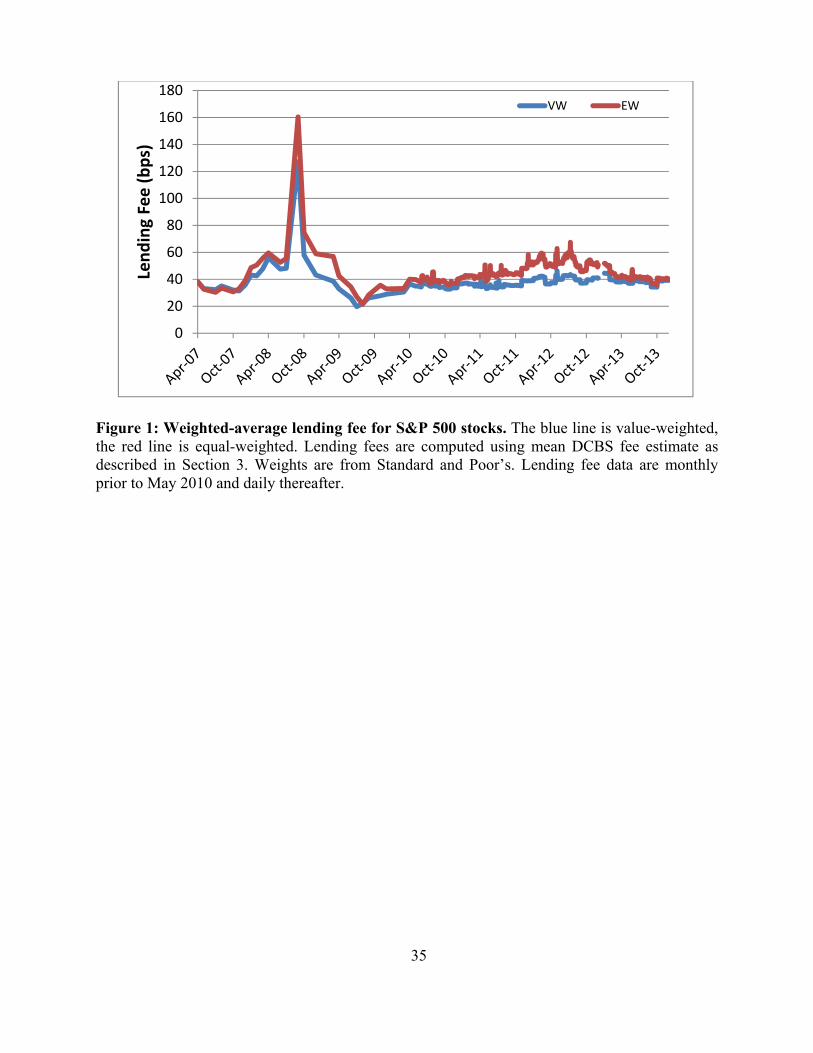
35

Figure 1: Weighted-average lending fee for S&P 500 stocks. The blue line is value-weighted, the red line is equal-weighted. Lending fees are computed using mean DCBS fee estimate as described in Section 3. Weights are from Standard and Poor’s. Lending fee data are monthly prior to May 2010 and daily thereafter.

0

20

40

60

80

100

120

140

160

180

Lend

ing Fee (bps)

VW EW

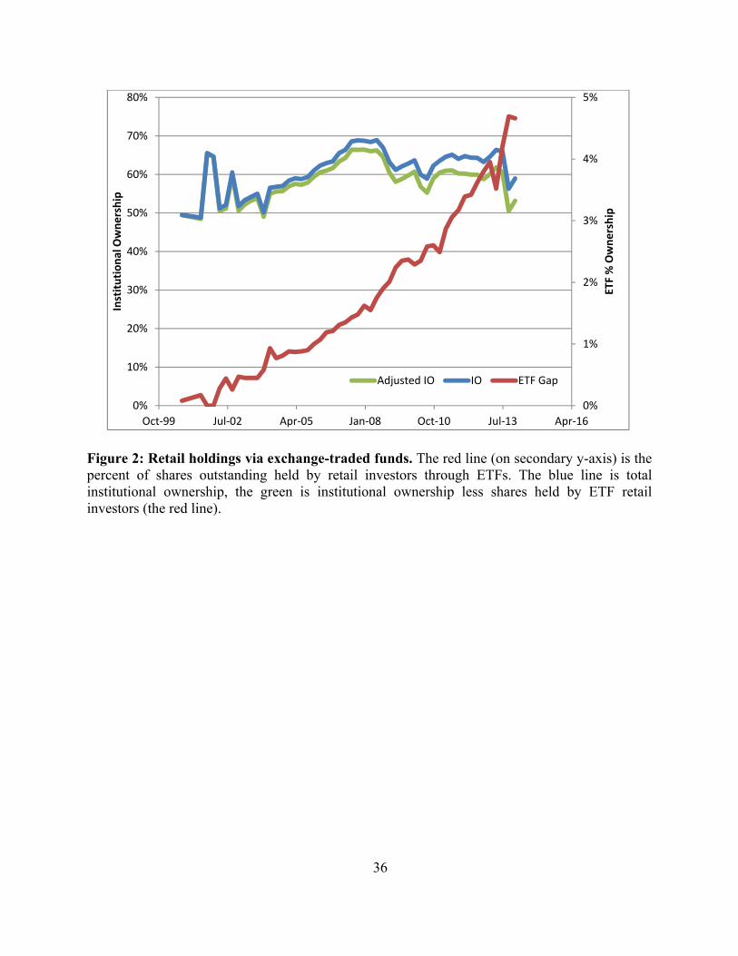
36

Figure 2: Retail holdings via exchange-traded funds. The red line (on secondary y-axis) is the percent of shares outstanding held by retail investors through ETFs. The blue line is total institutional ownership, the green is institutional ownership less shares held by ETF retail investors (the red line).

0%

1%

2%

3%

4%

5%

0%

10%

20%

30%

40%

50%

60%

70%

80%

Oct‐99 Jul‐02 Apr‐05 Jan‐08 Oct‐10 Jul‐13 Apr‐16

ETF % Owne

rship

Institu

tiona

l Owne

rship

Adjusted IO IO ETF Gap

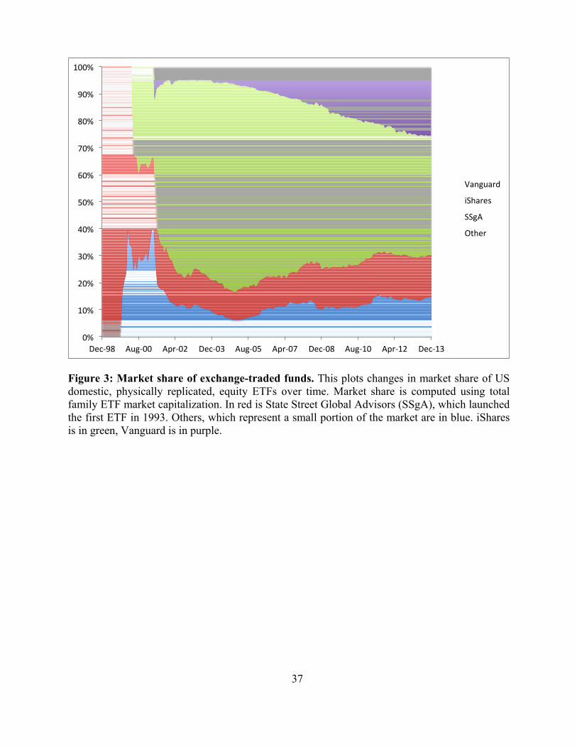
37

Figure 3: Market share of exchange-traded funds. This plots changes in market share of US domestic, physically replicated, equity ETFs over time. Market share is computed using total family ETF market capitalization. In red is State Street Global Advisors (SSgA), which launched the first ETF in 1993. Others, which represent a small portion of the market are in blue. iShares is in green, Vanguard is in purple.

0%

10%

20%

30%

40%

50%

60%

70%

80%

90%

100%

Dec‐98 Aug‐00 Apr‐02 Dec‐03 Aug‐05 Apr‐07 Dec‐08 Aug‐10 Apr‐12 Dec‐13

Vanguard

iShares

SSgA

Other

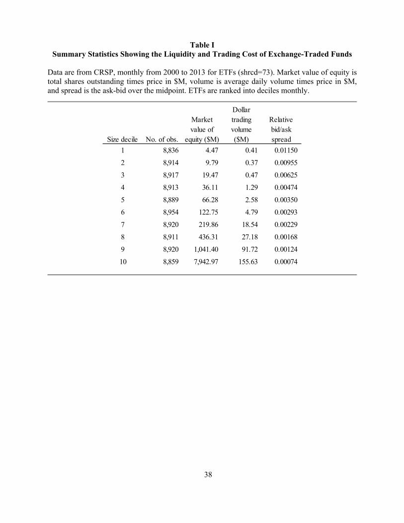
38

Table I Summary Statistics Showing the Liquidity and Trading Cost of Exchange-Traded Funds

Data are from CRSP, monthly from 2000 to 2013 for ETFs (shrcd=73). Market value of equity is total shares outstanding times price in $M, volume is average daily volume times price in $M, and spread is the ask-bid over the midpoint. ETFs are ranked into deciles monthly.

Size decile No. of obs.

Market value of

equity ($M)

Dollar trading volume ($M)

Relative bid/ask spread

1 8,836 4.47 0.41 0.01150 2 8,914 9.79 0.37 0.00955 3 8,917 19.47 0.47 0.00625 4 8,913 36.11 1.29 0.00474 5 8,889 66.28 2.58 0.00350 6 8,954 122.75 4.79 0.00293 7 8,920 219.86 18.54 0.00229 8 8,911 436.31 27.18 0.00168 9 8,920 1,041.40 91.72 0.00124 10 8,859 7,942.97 155.63 0.00074

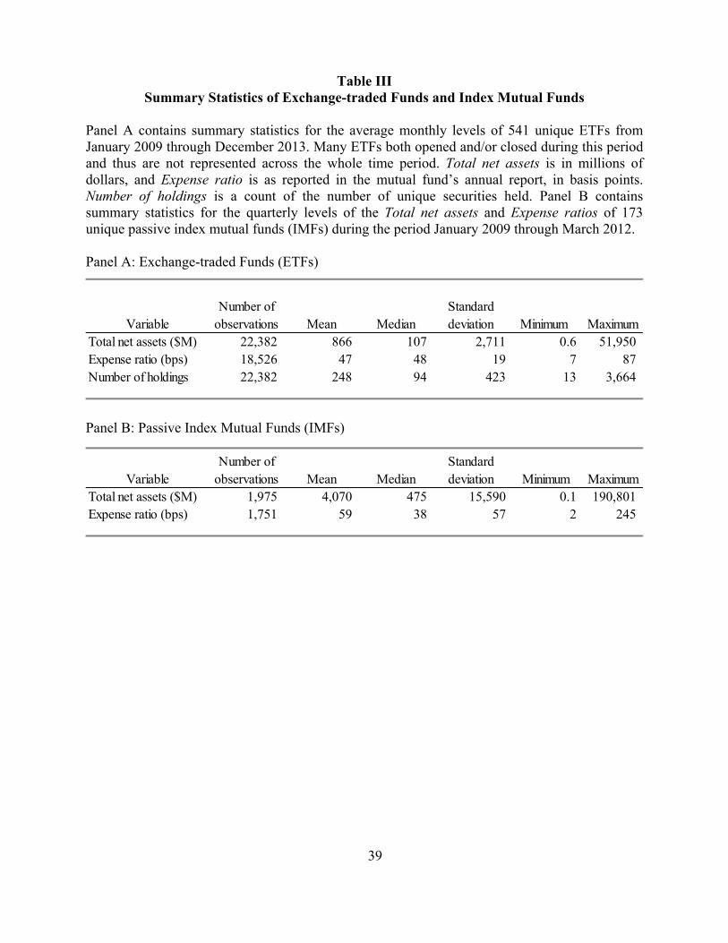
39

Table III Summary Statistics of Exchange-traded Funds and Index Mutual Funds

Panel A contains summary statistics for the average monthly levels of 541 unique ETFs from January 2009 through December 2013. Many ETFs both opened and/or closed during this period and thus are not represented across the whole time period. Total net assets is in millions of dollars, and Expense ratio is as reported in the mutual fund’s annual report, in basis points. Number of holdings is a count of the number of unique securities held. Panel B contains summary statistics for the quarterly levels of the Total net assets and Expense ratios of 173 unique passive index mutual funds (IMFs) during the period January 2009 through March 2012. Panel A: Exchange-traded Funds (ETFs)

Panel B: Passive Index Mutual Funds (IMFs)

Number of StandardVariable observations Mean Median deviation Minimum Maximum

Total net assets ($M) 22,382 866 107 2,711 0.6 51,950 Expense ratio (bps) 18,526 47 48 19 7 87 Number of holdings 22,382 248 94 423 13 3,664

Number of StandardVariable observations Mean Median deviation Minimum Maximum

Total net assets ($M) 1,975 4,070 475 15,590 0.1 190,801 Expense ratio (bps) 1,751 59 38 57 2 245

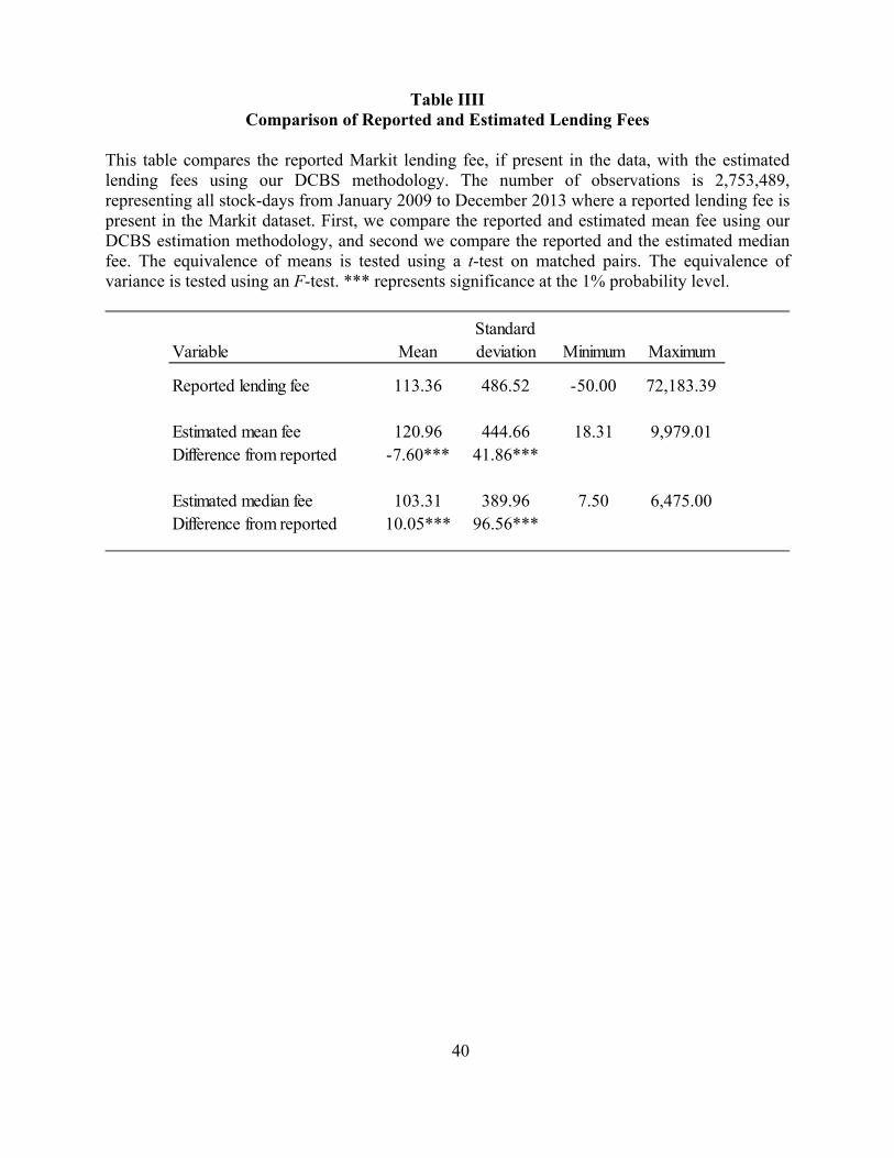
40

Table IIII Comparison of Reported and Estimated Lending Fees

This table compares the reported Markit lending fee, if present in the data, with the estimated lending fees using our DCBS methodology. The number of observations is 2,753,489, representing all stock-days from January 2009 to December 2013 where a reported lending fee is present in the Markit dataset. First, we compare the reported and estimated mean fee using our DCBS estimation methodology, and second we compare the reported and the estimated median fee. The equivalence of means is tested using a t-test on matched pairs. The equivalence of variance is tested using an F-test. *** represents significance at the 1% probability level.

StandardVariable Mean deviation Minimum Maximum

Reported lending fee 113.36 486.52 -50.00 72,183.39

Estimated mean fee 120.96 444.66 18.31 9,979.01Difference from reported -7.60*** 41.86***

Estimated median fee 103.31 389.96 7.50 6,475.00Difference from reported 10.05*** 96.56***

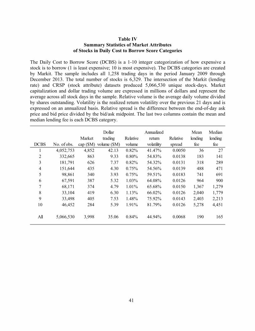
41

Table IV Summary Statistics of Market Attributes

of Stocks in Daily Cost to Borrow Score Categories The Daily Cost to Borrow Score (DCBS) is a 1-10 integer categorization of how expensive a stock is to borrow (1 is least expensive; 10 is most expensive). The DCBS categories are created by Markit. The sample includes all 1,258 trading days in the period January 2009 through December 2013. The total number of stocks is 6,329. The intersection of the Markit (lending rate) and CRSP (stock attribute) datasets produced 5,066,530 unique stock-days. Market capitalization and dollar trading volume are expressed in millions of dollars and represent the average across all stock days in the sample. Relative volume is the average daily volume divided by shares outstanding. Volatility is the realized return volatility over the previous 21 days and is expressed on an annualized basis. Relative spread is the difference between the end-of-day ask price and bid price divided by the bid/ask midpoint. The last two columns contain the mean and median lending fee is each DCBS category.

DCBS No. of obs.Market

cap ($M)

Dollar trading

volume ($M)Relative volume

Annualized return

volatilityRelative spread

Mean lending

fee

Median lending

fee1 4,052,753 4,852 42.13 0.82% 41.47% 0.0050 36 27 2 332,665 863 9.33 0.80% 54.83% 0.0138 183 141 3 181,791 626 7.37 0.82% 54.32% 0.0131 318 289 4 151,644 435 4.30 0.75% 54.56% 0.0139 488 471 5 98,861 340 3.93 0.75% 59.51% 0.0183 741 691 6 67,591 387 5.32 1.03% 64.08% 0.0126 964 900 7 68,171 374 4.79 1.01% 65.68% 0.0150 1,367 1,279 8 33,104 419 6.30 1.13% 66.02% 0.0126 2,040 1,779 9 33,498 405 7.53 1.48% 75.92% 0.0143 2,403 2,213

10 46,452 284 5.39 1.91% 81.79% 0.0126 5,278 4,451

All 5,066,530 3,998 35.06 0.84% 44.94% 0.0068 190 165

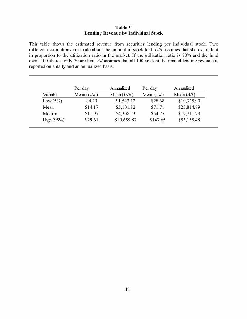
42

Table V Lending Revenue by Individual Stock

This table shows the estimated revenue from securities lending per individual stock. Two different assumptions are made about the amount of stock lent. Util assumes that shares are lent in proportion to the utilization ratio in the market. If the utilization ratio is 70% and the fund owns 100 shares, only 70 are lent. All assumes that all 100 are lent. Estimated lending revenue is reported on a daily and an annualized basis.

Per day Annualized Per day AnnualizedVariable Mean (Util ) Mean (Util ) Mean (All ) Mean (All )Low (5%) $4.29 $1,543.12 $28.68 $10,325.90Mean $14.17 $5,101.82 $71.71 $25,814.89Median $11.97 $4,308.73 $54.75 $19,711.79High (95%) $29.61 $10,659.82 $147.65 $53,155.48

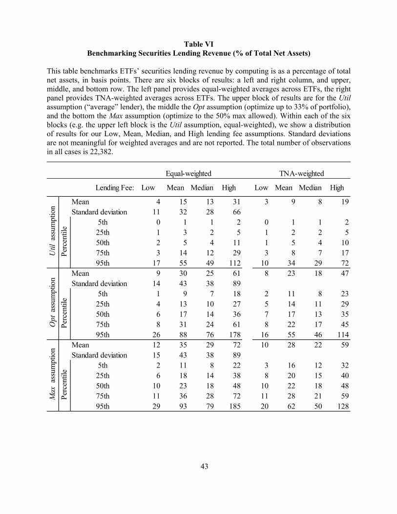
43

Table VI Benchmarking Securities Lending Revenue (% of Total Net Assets)

This table benchmarks ETFs’ securities lending revenue by computing is as a percentage of total net assets, in basis points. There are six blocks of results: a left and right column, and upper, middle, and bottom row. The left panel provides equal-weighted averages across ETFs, the right panel provides TNA-weighted averages across ETFs. The upper block of results are for the Util assumption (“average” lender), the middle the Opt assumption (optimize up to 33% of portfolio), and the bottom the Max assumption (optimize to the 50% max allowed). Within each of the six blocks (e.g. the upper left block is the Util assumption, equal-weighted), we show a distribution of results for our Low, Mean, Median, and High lending fee assumptions. Standard deviations are not meaningful for weighted averages and are not reported. The total number of observations in all cases is 22,382.

Lending Fee: Low Mean Median High Low Mean Median High

Mean 4 15 13 31 3 9 8 19Standard deviation 11 32 28 66

5th 0 1 1 2 0 1 1 225th 1 3 2 5 1 2 2 550th 2 5 4 11 1 5 4 1075th 3 14 12 29 3 8 7 1795th 17 55 49 112 10 34 29 72

Mean 9 30 25 61 8 23 18 47Standard deviation 14 43 38 89

5th 1 9 7 18 2 11 8 2325th 4 13 10 27 5 14 11 2950th 6 17 14 36 7 17 13 3575th 8 31 24 61 8 22 17 4595th 26 88 76 178 16 55 46 114

Mean 12 35 29 72 10 28 22 59Standard deviation 15 43 38 89

5th 2 11 8 22 3 16 12 3225th 6 18 14 38 8 20 15 4050th 10 23 18 48 10 22 18 4875th 11 36 28 72 11 28 21 5995th 29 93 79 185 20 62 50 128

Equal-weighted TNA-weighted

Util

ass

umpt

ion

Opt

ass

umpt

ion

Max

ass

umpt

ion

Perc

entil

ePe

rcen

tile

Perc

entil

e

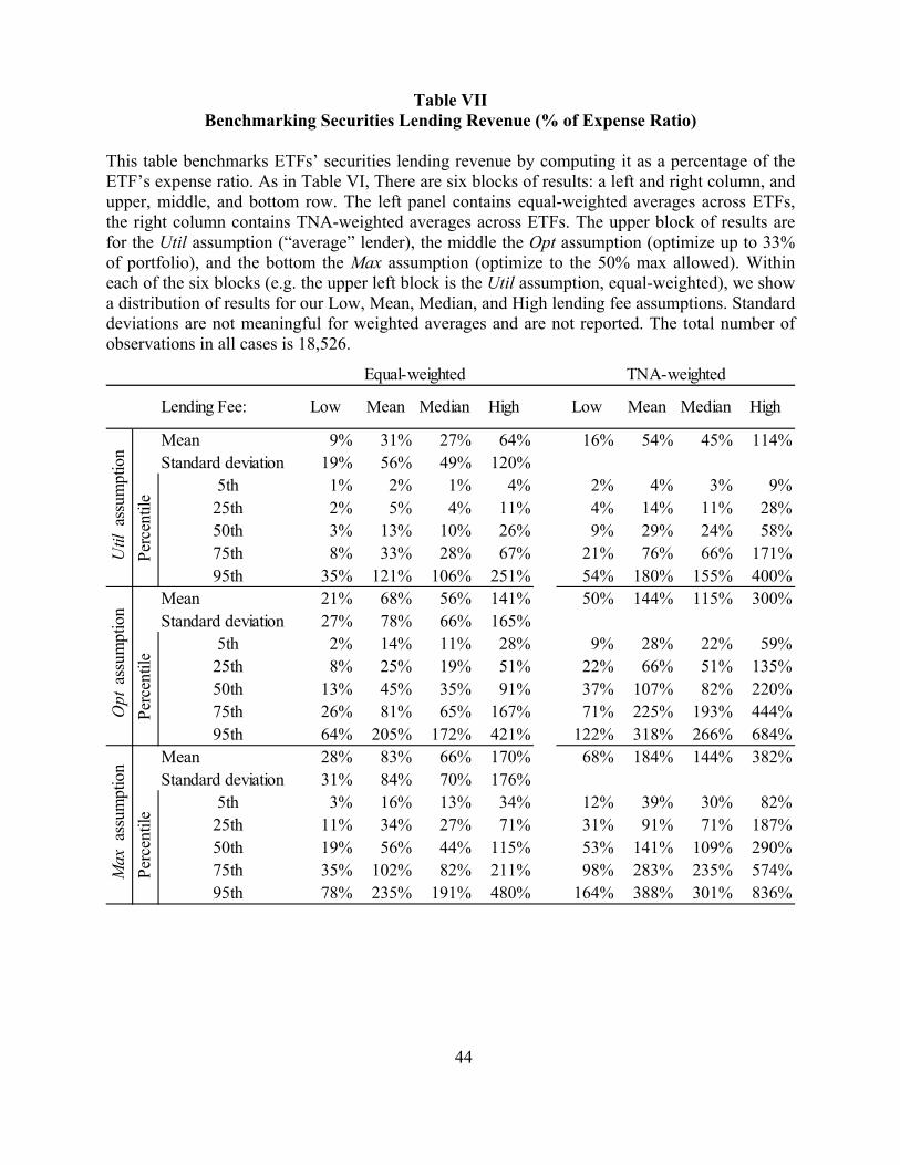
44

Table VII Benchmarking Securities Lending Revenue (% of Expense Ratio)

This table benchmarks ETFs’ securities lending revenue by computing it as a percentage of the ETF’s expense ratio. As in Table VI, There are six blocks of results: a left and right column, and upper, middle, and bottom row. The left panel contains equal-weighted averages across ETFs, the right column contains TNA-weighted averages across ETFs. The upper block of results are for the Util assumption (“average” lender), the middle the Opt assumption (optimize up to 33% of portfolio), and the bottom the Max assumption (optimize to the 50% max allowed). Within each of the six blocks (e.g. the upper left block is the Util assumption, equal-weighted), we show a distribution of results for our Low, Mean, Median, and High lending fee assumptions. Standard deviations are not meaningful for weighted averages and are not reported. The total number of observations in all cases is 18,526.

Lending Fee: Low Mean Median High Low Mean Median High

Mean 9% 31% 27% 64% 16% 54% 45% 114%Standard deviation 19% 56% 49% 120%

5th 1% 2% 1% 4% 2% 4% 3% 9%25th 2% 5% 4% 11% 4% 14% 11% 28%50th 3% 13% 10% 26% 9% 29% 24% 58%75th 8% 33% 28% 67% 21% 76% 66% 171%95th 35% 121% 106% 251% 54% 180% 155% 400%

Mean 21% 68% 56% 141% 50% 144% 115% 300%Standard deviation 27% 78% 66% 165%

5th 2% 14% 11% 28% 9% 28% 22% 59%25th 8% 25% 19% 51% 22% 66% 51% 135%50th 13% 45% 35% 91% 37% 107% 82% 220%75th 26% 81% 65% 167% 71% 225% 193% 444%95th 64% 205% 172% 421% 122% 318% 266% 684%

Mean 28% 83% 66% 170% 68% 184% 144% 382%Standard deviation 31% 84% 70% 176%

5th 3% 16% 13% 34% 12% 39% 30% 82%25th 11% 34% 27% 71% 31% 91% 71% 187%50th 19% 56% 44% 115% 53% 141% 109% 290%75th 35% 102% 82% 211% 98% 283% 235% 574%95th 78% 235% 191% 480% 164% 388% 301% 836%

Equal-weighted TNA-weighted

Util

ass

umpt

ion

Opt

ass

umpt

ion

Max

ass

umpt

ion

Perc

entil

ePe

rcen

tile

Perc

entil

e

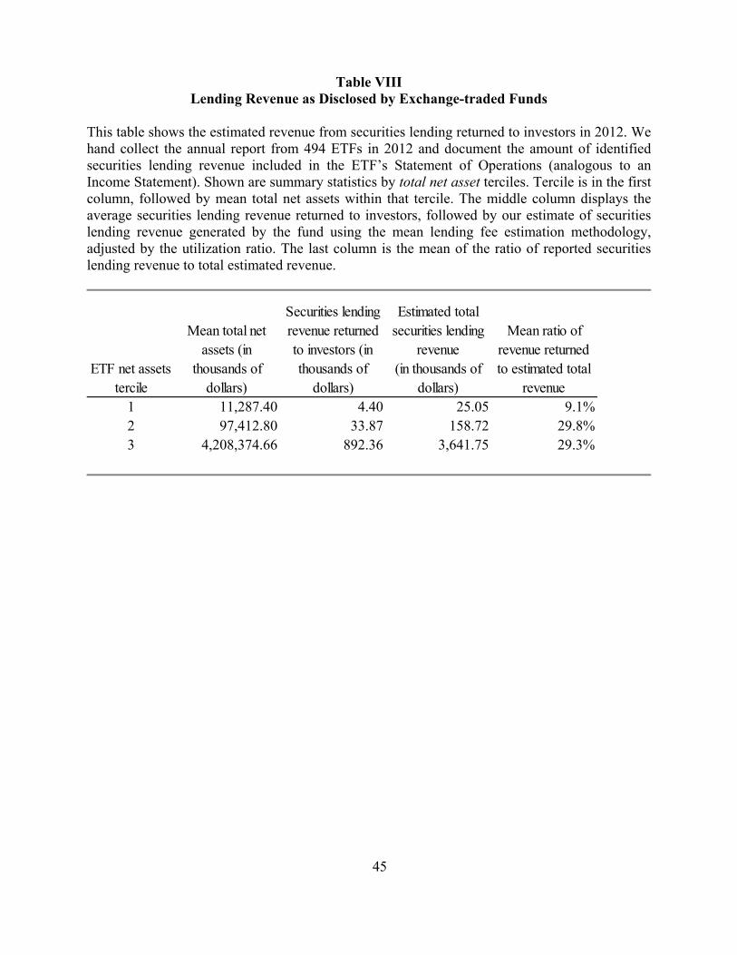
45

Table VIII Lending Revenue as Disclosed by Exchange-traded Funds

This table shows the estimated revenue from securities lending returned to investors in 2012. We hand collect the annual report from 494 ETFs in 2012 and document the amount of identified securities lending revenue included in the ETF’s Statement of Operations (analogous to an Income Statement). Shown are summary statistics by total net asset terciles. Tercile is in the first column, followed by mean total net assets within that tercile. The middle column displays the average securities lending revenue returned to investors, followed by our estimate of securities lending revenue generated by the fund using the mean lending fee estimation methodology, adjusted by the utilization ratio. The last column is the mean of the ratio of reported securities lending revenue to total estimated revenue.

ETF net assets tercile

Mean total net assets (in

thousands of dollars)

Securities lending revenue returned to investors (in thousands of

dollars)

Estimated total securities lending

revenue(in thousands of

dollars)

Mean ratio of revenue returned to estimated total

revenue1 11,287.40 4.40 25.05 9.1%2 97,412.80 33.87 158.72 29.8%3 4,208,374.66 892.36 3,641.75 29.3%

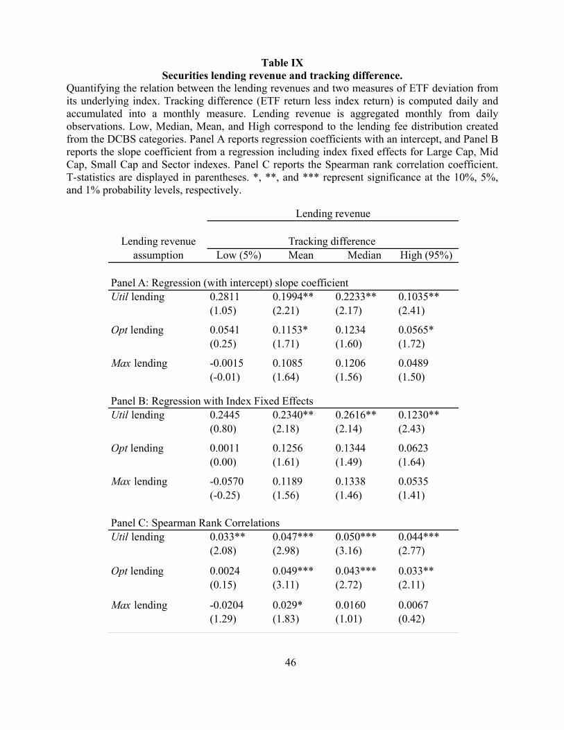
46

Table IX Securities lending revenue and tracking difference.

Quantifying the relation between the lending revenues and two measures of ETF deviation from its underlying index. Tracking difference (ETF return less index return) is computed daily and accumulated into a monthly measure. Lending revenue is aggregated monthly from daily observations. Low, Median, Mean, and High correspond to the lending fee distribution created from the DCBS categories. Panel A reports regression coefficients with an intercept, and Panel B reports the slope coefficient from a regression including index fixed effects for Large Cap, Mid Cap, Small Cap and Sector indexes. Panel C reports the Spearman rank correlation coefficient. T-statistics are displayed in parentheses. *, **, and *** represent significance at the 10%, 5%, and 1% probability levels, respectively.

Lending revenueassumption Low (5%) Mean Median High (95%)

Panel A: Regression (with intercept) slope coefficientUtil lending 0.2811 0.1994** 0.2233** 0.1035**

(1.05) (2.21) (2.17) (2.41)

Opt lending 0.0541 0.1153* 0.1234 0.0565*(0.25) (1.71) (1.60) (1.72)

Max lending -0.0015 0.1085 0.1206 0.0489(-0.01) (1.64) (1.56) (1.50)

Panel B: Regression with Index Fixed EffectsUtil lending 0.2445 0.2340** 0.2616** 0.1230**

(0.80) (2.18) (2.14) (2.43)

Opt lending 0.0011 0.1256 0.1344 0.0623(0.00) (1.61) (1.49) (1.64)

Max lending -0.0570 0.1189 0.1338 0.0535(-0.25) (1.56) (1.46) (1.41)

Panel C: Spearman Rank CorrelationsUtil lending 0.033** 0.047*** 0.050*** 0.044***

(2.08) (2.98) (3.16) (2.77)

Opt lending 0.0024 0.049*** 0.043*** 0.033**(0.15) (3.11) (2.72) (2.11)

Max lending -0.0204 0.029* 0.0160 0.0067(1.29) (1.83) (1.01) (0.42)

Lending revenue

Tracking difference

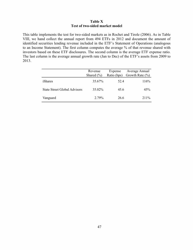
47

Table X Test of two-sided market model

This table implements the test for two-sided markets as in Rochet and Tirole (2006). As in Table VIII, we hand collect the annual report from 494 ETFs in 2012 and document the amount of identified securities lending revenue included in the ETF’s Statement of Operations (analogous to an Income Statement). The first column computes the average % of that revenue shared with investors based on these ETF disclosures. The second column is the average ETF expense ratio. The last column is the average annual growth rate (Jan to Dec) of the ETF’s assets from 2009 to 2013.

RevenueShared (%)

ExpenseRatio (bps)

Average Annual Growth Rate (%)

iShares 35.67% 52.4 116%

State Street Global Advisors 35.02% 45.6 45%

Vanguard 2.79% 26.6 211%

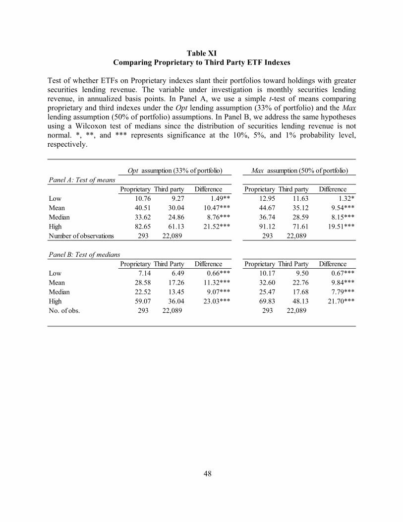
48

Table XI

Comparing Proprietary to Third Party ETF Indexes

Test of whether ETFs on Proprietary indexes slant their portfolios toward holdings with greater securities lending revenue. The variable under investigation is monthly securities lending revenue, in annualized basis points. In Panel A, we use a simple t-test of means comparing proprietary and third indexes under the Opt lending assumption (33% of portfolio) and the Max lending assumption (50% of portfolio) assumptions. In Panel B, we address the same hypotheses using a Wilcoxon test of medians since the distribution of securities lending revenue is not normal. *, **, and *** represents significance at the 10%, 5%, and 1% probability level, respectively.

Panel A: Test of meansProprietary Third party Difference Proprietary Third party Difference

Low 10.76 9.27 1.49** 12.95 11.63 1.32*Mean 40.51 30.04 10.47*** 44.67 35.12 9.54***Median 33.62 24.86 8.76*** 36.74 28.59 8.15***High 82.65 61.13 21.52*** 91.12 71.61 19.51***Number of observations 293 22,089 293 22,089

Panel B: Test of mediansProprietary Third Party Difference Proprietary Third Party Difference

Low 7.14 6.49 0.66*** 10.17 9.50 0.67***Mean 28.58 17.26 11.32*** 32.60 22.76 9.84***Median 22.52 13.45 9.07*** 25.47 17.68 7.79***High 59.07 36.04 23.03*** 69.83 48.13 21.70***No. of obs. 293 22,089 293 22,089

Opt assumption (33% of portfolio) Max assumption (50% of portfolio)

49

Table XII Comparing ETF Weights to Index Weights (third party indexes)

Test of whether ETFs tracking third party (fully transparent) indexes slant their portfolios toward holdings with greater securities lending revenue. Regression is of first differences (all variables), at the individual holdings level. The dependent variable is Delta ETF weight – Index weight. Lending fee is computed from DCBS distribution, where the mean is used. Relative spread is the difference between the ask and bid prices divided by the bid/ask midpoint. Market Cap is price times shares outstanding, Volume is daily shares traded times closing price, Amihud liquidity is as defined in Amihud (2002), and Idiosyncratic volatility is computed over the past 22 days based on a Fama-French 3 factor model. Standard errors are clustered by ETF-CUSIP and robust to heteroskedasticity within each cluster. Models 1 and 2 use the whole sample, Models 3 and 4 look at the subset where the DCBS bin changes (either up or down) and models 5 and 6 eliminates DCBS bin 1, which is most of the sample and where stocks are very inexpensive to borrow. Values in parentheses are t-ratios. *, **, and *** represent significance at the 10%, 5%, and 1% probability levels, respectively.

(1) (2) (3) (4) (5) (6)Delta Delta Delta Delta Delta Delta

Lending fee (Mean) 0.5113* 0.5198* 0.5450* 0.5456* 0.5550* 0.5519*(1.74) (1.77) (1.83) (1.73) (1.76) (1.75)

Relative spread 0.6948** 0.6895** 3.4215 5.2274* -2.1947** -2.1929**(2.30) (2.29) (1.26) (1.68) (-2.27) (-2.21)

Market Cap -0.0001*** -0.0001*** -0.0001** -0.0001* -0.0001 -0.0001(-5.14) (-5.15) (-2.11) (-1.94) (-1.50) (-1.52)

Volume ($) -0.1235 -0.1191 -0.1165 -0.0445 -0.0901 -0.0755(-0.59) (-0.57) (-0.45) (-0.17) (-0.60) (-0.50)

Amihud Liquidity 0.0424 0.0330 -0.0144 -0.0113 -0.0048* -0.0047(1.34) (1.13) (-1.56) (-1.16) (-1.76) (-1.58)

Idiosyncratic Volatility 1.0681*** 1.0547*** 2.0130 2.3414 0.2109 0.2673(2.75) (2.70) (1.32) (1.48) (0.44) (0.57)

Whole Sample Change in DCBS only No general collateral

Constant 0.0001 -0.1139 0.0002 -0.0950* 0.0005 1.0204***(0.12) (-0.18) (0.03) (-1.73) (0.20) (3.66)

Observations 3,723,987 3,723,987 12,888 12,888 83,739 83,739R-squared 0.00 0.00 0.00 0.01 0.00 0.00Clusters 9,386 9,386 1,249 1,249 955 955Time dummies No Yes No Yes No Yes

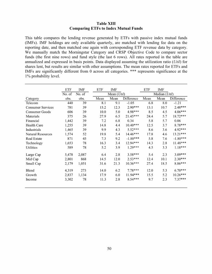
50

Table XIII Comparing ETFs to Index Mutual Funds

This table compares the lending revenue generated by ETFs with passive index mutual funds (IMFs). IMF holdings are only available quarterly, are matched with lending fee data on the reporting date, and then matched one again with corresponding ETF revenue data by category. We manually match the Morningstar Category and CRSP Objective Code to compare sector funds (the first nine rows) and fund style (the last 6 rows). All rates reported in the table are annualized and expressed in basis points. Data displayed assuming the utilization ratio (Util) for shares lent, but results are similar with other assumptions. The mean rates reported for ETFs and IMFs are significantly different from 0 across all categories. *** represents significance at the 1% probability level.