Embed Size (px)
Citation preview

NBER WORKING PAPER SERIES
TWO REASONS WHY MONEY AND CREDIT MAY BE USEFUL IN MONETARYPOLICY
Lawrence ChristianoRoberto Motto
Massimo Rostagno
Working Paper 13502http://www.nber.org/papers/w13502
NATIONAL BUREAU OF ECONOMIC RESEARCH1050 Massachusetts Avenue
Cambridge, MA 02138October 2007
Paper presented at the Fourth ECB Central Banking Conference, The Role of Money: Money andMonetary Policy in the Twenty-First Century," Frankfurt, November 9-10, 2006. We would like tothank Claudio Borio, Dale Henderson, John Leahy, Andy Levin, Christian Noyer, Lars Svensson andHarald Uhlig for helpful discussions. The views expressed in this paper do not necessarily reflect theviews of the European Central Bank.
© 2007 by Lawrence Christiano, Roberto Motto, and Massimo Rostagno. All rights reserved. Shortsections of text, not to exceed two paragraphs, may be quoted without explicit permission providedthat full credit, including © notice, is given to the source.

Two Reasons Why Money and Credit May be Useful in Monetary PolicyLawrence Christiano, Roberto Motto, and Massimo RostagnoNBER Working Paper No. 13502October 2007JEL No. E41,E44,E52,E58
ABSTRACT
We describe two examples which illustrate in different ways how money and credit may be usefulin the conduct of monetary policy. Our first example shows how monitoring money and credit canhelp anchor private sector expectations about inflation. Our second example shows that a monetarypolicy that focuses too narrowly on inflation may inadvertently contribute to welfare-reducing boom-bustcycles in real and financial variables. The example is of some interest because it is based on a monetarypolicy rule fit to aggregate data. We show that a policy of monetary tightening when credit growthis strong can mitigate the problems identified in our second example.
Lawrence ChristianoDepartment of EconomicsNorthwestern University2003 Sheridan RoadEvanston, IL 60208and [email protected]
Roberto MottoEuropean Central BankPostfach 16 03 19D-60066 Frankfurt am [email protected]
Massimo RostagnoEuropean Central BankPostfach 16-03-19D-60066 Frankfurt am [email protected]

1. Introduction
The current consensus is that money and credit have essentially no constructive role
to play in monetary policy. When Michael Woodford first suggested this possibility
before a large gathering of prominent economists in Mexico city in 1996, the audience
was mystified (Woodford, 1998). The consensus at the time was the one forged by
Milton Friedman, according to which inflation is ‘always and everywhere a monetary
phenomenon’. The pendulum has now swung to the other extreme, in the form of a
new consensus which de-emphasizes money completely. We briefly review the reasons
for this shift, before presenting two examples which suggest the pendulum may have
swung too far.
The experience of the 1970s showed that the inflation expectations of the public
can lose their anchor and that when this happens the social costs are high. To stabi-
lize inflation expectations, monetary authorities have evolved versions of the following
policy: When the evidence suggests that inflation will rise above some numerical ob-
jective, the monetary authority responds proactively by tightening monetary policy.
Monetary policy is loosened in response to signs that inflation will fall below the nu-
merical objective.1 A rough characterization of such a policy expresses the interest
rate, Rt, as a function of expected inflation, πet+1, and other variables, xt :
Rt = ρRt−1 + (1− ρ)£απ
¡πet+1 − π∗t
¢+ αxxt
¤. (1.1)
1In practice, monetary policy strategies differ according to how vigorously the central bank
responds to changing signals about future inflation, and how much weight it assigns to other factors,
such as the state of the real economy. Strategies also differ according to how heavily they make use
of formal econometric models of the economy. In recent years, there has been much progress towards
integrating formal models into the design of monetary policy. For example, Giannoni and Woodford
(2005), Svensson and Tetlow (2005), and Svensson and Woodford (2005) propose replacing (1.1) by
the optimal policy relative to a specified objective function.
2

Here, π∗t denotes the monetary authority’s inflation target. When ρ > 0, policy
acts to minimize large movements in the interest rate from one period to the next.2
Although we have included only the one-period-ahead forecast of inflation in this
rule, what we have to say goes through in the more plausible case where central bank
policy is driven by the longer-term outlook for inflation. We will refer to the rule as a
Taylor rule, though that is not strictly speaking accurate since the rule John Taylor
discusses reacts only to current inflation and output. We chose to include expected
inflation in (1.1) to account for the fact that in practice monetary authorities must
anticipate economic developments in advance, since policy actions may have very
little immediate impact and thus may take time to exert their influence on the
economy.3 We do not mean to suggest that any central bank’s policy is governed by
a rigid rule like (1.1). We think of (1.1) only as a rough characterization, one that
allows us to make our points about the role of money and credit in monetary policy.
There are two reasons for the current consensus that money and credit have es-
sentially no role to play in monetary policy. First, these variables are not included
in (1.1). Second, monetary theory lends some support to the notion that money
demand and supply are virtually irrelevant in determining the operating character-
istics of (1.1). For intuition, recall the undergraduate textbook IS-LM model with
an aggregate supply side. In this model, money balances do not enter the spending
decisions underlying the IS curve, and they do not enter the considerations deter-
mining the supply curve. If monetary policy is characterized by an interest rate rule
like (1.1), then the equilibrium of the model is determined independently of the LM
curve.4 That is, the operating characteristics of (1.1) can be studied without taking
2For a rationale, see Woodford (2003b).3This point was stressed by Svensson (1997).4The notion that money balances literally do not interact with consumption and investment
3

a stand on the nature of money demand or money supply.5
In what follows we present two examples in which a strategy such as (1.1) is not
successful at stabilizing the economy. In each example outcomes are improved if: (a)
the central bank carefully monitors monetary indicators and (b) it reacts or threatens
to react to such indicators in case inflation expectations or asset price formation get
out of control. By "monetary indicators" we mean aggregates defined both on the
liability (i.e. money proper) and the asset side (i.e. credit) of monetary institutions.
After presenting the examples, we provide some concluding remarks. An appendix
discusses our first example in greater detail.
2. First Example: Anchoring Inflation Expectations
Our first example illustrates points emphasized by Benhabib, Schmitt-Grohe and
Uribe (2001,2002a,b), Carlstrom and Fuerst (2002,2005) and Christiano and Ros-
decisions is implausible. Most theories of money demand rest on the premise that money bal-
ances play a role in facilitating transactions and that money balances therefore do interact with
other decisions. However, experience has shown that those theories also imply that the role of
money in consumption, investment and employment dedisions is quantitatively negligible (See, for
example, McCallum, 2001.) That is, the insight based on the textbook macro model that one can
ignore money demand and money supply when monetary policy is governed by (1.1) is a very good
approximation in a broad class of models.5A third reason that is sometimes given for ignoring money demand is that money demand is
unstable. This overstates the instability of money demand and understates the stability of non-
financial variables. A simple graph of the money velocity based on the St. Louis Fed’s measure of
transactions balances, MZM, against the interest rate shows a reasonably stable relation. At the
same time, the US consumption to output ratio suddenly began to trend up since the early 1980s,
and is now about 6 percentage points of GDP higher than it used to be. This change in trend
almost fully explains a similar change in trend in the US current account. No one would suggest
not looking at the current account, consumption or GDP because of this evidence of instability.
4

tagno (2001) (BSU-CF-CR). Although (1.1) may be effective at anchoring inflation
expectations in some models, the finding is not robust to small, empirically plausi-
ble, changes in model specification. This is of concern because there is considerable
uncertainty about the correct model specification.
We begin by discussing why (1.1) is effective in anchoring inflation expectations
in the simple New-Keynesian model.6 We then introduce a slight modification to
the environment which captures in spirit of many of the examples in BSU-CF-CR.
The modification is motivated by the evidence that firms need to borrow substantial
amounts of working capital to finance variable inputs like labor and intermediate
goods.7 This modification introduces a supply-side channel for monetary policy and
creates the possibility for inflation expectations to lose their anchor. This is so,
even if monetary policy acts aggressively against inflation by assigning a high value
to απ in (1.1). The resulting instability affects all the variables in the model, in-
cluding money and credit. A commitment by the monetary authority to monitor
these variables and to react when they exhibit instability that is not clearly linked
6As Benhabit, Schmitt-Grohe and Uribe (2001) note, even in this model there is a global problem
of multiple equilibria. In addition to the ‘normal’ equilibrium, there is another equilibrium in which
the interest rate drops to zero. However, an escape clause strategy in which the monetary authority
commits to deviating from (1.1) to a policy of controlling the money supply in the event that the
interest rate drops to zero eliminates this equilibrium in many models. This observation reinforces
our basic point that money may have a constructive role to play in monetary policy. For further
discussion, see Christiano and Rostagno (2001).7See, for example, Christiano, Eichenbaum and Evans (1996) and Barth and Ramey (2002). The
existence of a supply-side channel for monetary policy is potentially an explanation for the ‘price
puzzle’, the finding in structural vector autoregressions that inflation tends to rise for a while after
a monetary tightening (see Christiano, Eichenbaum, and Evans, 1999). Additional evidence on the
importance of the supply-side channel is provided in the appendix.
5

to fundamental economic shocks (including money demand shocks) keeps inflation
expectations anchored within a narrow range. In effect, the strategy corresponds
to operating monetary policy according to (1.1) with a particular ‘escape clause’: a
commitment to control money and credit aggregates directly in case these variables
misbehave. The strategy works like the textbook analysis of a bank run. The gov-
ernment’s commitment to supply liquidity in the event of a bank run eliminates the
occurrence of a bank run in the first place, so that government never has to act on
its commitment. Similarly, the monetary authority’s commitment to monitor money
growth and reign it in if necessary implies that inflation expectations and thus money
growth never get out of line in the first place.
Here, we provide an intuitive discussion. A formal, numerical analysis is pre-
sented in the appendix. Suppose that the economy is described by the IS-LM model
augmented by a supply curve, as in Figure 1. On the vertical axis of Figure 1a, we
display the nominal rate of interest and on the horizontal axis appears aggregate real
output, y. Note that the IS curve is a function of expected inflation because the
spending decisions summarized in that curve are a function of the real interest rate.
The LM curve summarizes money market equilibrium in the usual way. Figure 1b
displays the supply side of the economy, in which higher output is associated with
higher inflation. The curve captures the idea that higher output raises pressure on
scarce resources, driving up production costs and leading businesses to post higher
prices.
Suppose that monetary policy responds to a one percentage point rise in expected
inflation, πe, by raising the nominal rate of interest by more than one percentage point
(the ‘Taylor principle’). It is easy to see that a monetary authority which follows the
Taylor principle in the simple model of Figure 1 succeeds in anchoring the public’s
expectations about inflation. In particular, suppose a belief begins to circulate that
6

inflation will rise, so that πe jumps. The monetary authority reacts by reducing the
money supply so that the nominal rate of interest rises by more than the rise in πe
(see Figure 1a). The resulting shift up in the LM curve causes output to fall from y1
to y2. The fall in output, by reducing costs, leads to a fall in inflation (Figure 1b).
Thus, in the given model and under the given monetary policy, a spontaneous jump
in expected inflation produces a chain of events that ultimately places downward
pressure on actual inflation. Under these circumstances, a general fear that inflation
will rise could not persist for long. Thus, inflation expectations are anchored under
the Taylor principle in the given model.
To see how crucial the Taylor principle is for anchoring inflation expectations
in the model of Figure 1, suppose the monetary authority did not apply the Taylor
principle. That is, the monetary authority responds to a one percent rise in expected
inflation by raising the nominal rate of interest by less than one percent. In terms
of Figure 1, this means that the monetary authority shifts the LM curve up by less
than the rise in πe. The resulting fall in the real rate of interest implies an increase in
spending. The rise in spending leads to a rise in output and, hence, costs. The rise
in costs in turn places upward pressure on inflation. In this way a rise in expected
inflation initiates a chain of events that ultimately produces a rise in actual inflation.
The outcome is that inflation expectations are self-fulfilling and have no anchor.
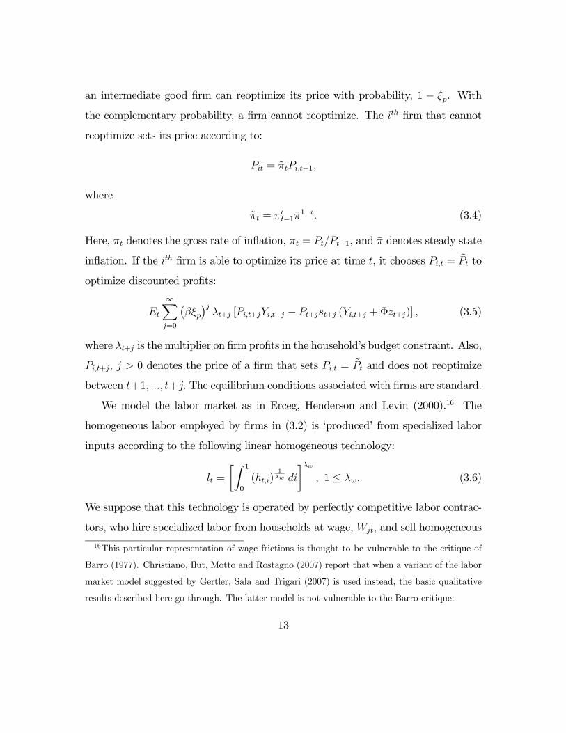
Now consider the modification to the economy that we mentioned in the intro-
duction. In particular, suppose that when the nominal interest rate is increased,
the output-inflation trade-off shifts up (see Figure 2b). This could occur because an
increase in the interest rate directly increases the cost of production by raising ex-
penses associated with financing inventories, the wage bill and other variable costs.8
8We cite evidence in the appendix which indicates borrowing for variable inputs may be sub-
stantial in practice.
7

Prices might also rise as a by-product of the tightening in balance sheets that occurs
as higher interest rates drive asset values down. Suppose, as before, that inflation
expectations rise and the monetary authority follows the Taylor principle. The mon-
etary authority shifts the LM curve up by more than the amount of the increase in
πe, so that the real rate of interest rises. Spending falls. If the supply curve did
not shift, then our previous analysis indicates that actual inflation would fall and
the higher πe would not be confirmed. But, under the modified scenario tightening
monetary conditions produce such a substantial rise in costs that actual inflation
rises. In this scenario, a rise in inflation expectations produces a chain of events that
ultimately results in higher inflation. The outcome is that, despite the application
of the Taylor principle, inflation expectations have no anchor.
It is asking too much of our simple diagrams to use them to think through what
happens over time when inflation expectations have lost their anchor. For this, an
explicit dynamic equilibrium model is required. The analyses reported in BSU-CF-
CR do this, and there we see that when things go wrong all economic variables
fluctuate over time in response to non-fundamental economic shocks. Among these
variables is the money supply. It is shown that a monetary policy which commits
to deviating from the Taylor rule as soon as money is observed to respond to non-
fundamental shocks in effect anchors inflation expectations.9 To implement this
policy requires a public commitment to monitor the money supply carefully and to
expend resources analyzing the reasons for its fluctuations. Paradoxically, in practice
it will seem like the monitoring policy is pointless.
A concluding remark about this example deserves emphasis. According to the
theoretical analyses that support the idea of an escape clause strategy, all variables
9It is possible to construct examples in which even this policy will not anchor expectations,
though these examples seem unlikely. For further discussion, see Christiano and Rostagno (2001).
8

in the economy exhibit instability when inflation expectations lose their anchor.
The models imply that an escape clause strategy which abandons (1.1) in favor of
stabilizing any economic variable - not necessarily money per se - works equally
well. When we conclude that the right variable to control in the event that the
escape clause is activated is money, we introduce considerations that lie outside the
models. Economic models assume that the monetary authority has perfect control
over any one variable in the economy with its one policy instrument. It can control
money as easily as the current account or Gross National Product. In reality, there
is only one variable that the monetary authority controls directly and credibly, and
that is money. All other variables that it may attempt to control - the interest
rate, the current account, etc. - can only be controlled indirectly, by virtue of the
monetary authority’s control of the money supply.10 What is crucial for the escape
clause strategy to work is that the central bank be able to credibly control whatever
variable it commits to control in the event that the escape clause is activated. In
practice, there really is only one such variable: money.
3. Second Example: Asset Market Volatility
Our second example summarizes the analysis of Christiano, Ilut, Motto and Ros-
tagno (2007). This example builds on the analysis of Beaudry and Portier (2004,
2006), which suggests that a substantial fraction of economic fluctuations may be
triggered by the arrival of signals about future improvements in productivity. We
find that when such a signal shock is fed to a standard model used in the analysis
of business cycles, it produces patterns that in many ways resembles the boom-bust
10The monetary aggregate directly controlled by the US Federal Reserve is the nonborrowed
reserves of banks.
9

cycles that economies experience periodically.11 In the model, the response of invest-
ment, consumption, output and stock prices greatly exceed what is socially efficient.
The excess volatility reflects two features of the model: (i) there are frictions in the
setting of wages and (ii) monetary policy focuses too narrowly on inflation. The
finding should be cause for concern, because there is substantial evidence that wage
frictions are important and because the monetary policy rule used in our analysis is
a version of (1.1) in which the parameters have been estimated using aggregate data.
Because the nominal wage rate is relatively sticky in the model, an overly narrow
focus on inflation stabilization in effect reduces to real wage stabilization. Such a
policy produces bad outcomes because it interferes with the efficient allocation of
resources. Although this is well known as a matter of principle (see, e.g., Erceg,
Henderson and Levin, 2000), what is less well known is that is that a policy rule
like (1.1) can make the monetary authorities unwitting participants in boom-bust
episodes. Although additional empirical research is necessary, there is indirect ev-
idence consistent with the view that a narrow focus on inflation stabilization may
produce instability. For example, Cecchetti and Ehrmann (2002) present evidence
that suggests that adopting an inflation targeting monetary regime may increase
output volatility.12
11We use a variant of the model proposed in Christiano, Eichenbaum and Evans (2005) and
further analyzed in Smets and Wouters (2003, 2007).12Several countries refocused their monetary policy more narrowly on inflation by formally adopt-
ing inflation targeting in the 1980s and 1990s. To isolate the impact of this policy change on output
volatility, one has to disentangle the effects of the change from the effects of all the other factors
that produced a moderation in volatility in this period (the ‘Great Moderation’). Cecchetti and
Ehrmann (2002) do this by computing the standard deviation of output growth in countries that
adopted inflation targeting and in countries that are non-targeters. They report that the average
volatility across non-targeters in the 1985-1989 period and the 1993-1997 period is 10.12 and 7.41,
10

There is a long tradition which locates the cause of boom-bust cycles in excessive
credit creation. A recent review of this tradition, and some evidence to support
it, is provided in Eichengreen and Mitchener (2004).13 Motivated by this strand of
literature, we introduce credit into our model. We do this by introducing frictions into
the financing of capital, following the lead of Bernanke, Gertler and Gilchrist (1999).
We find that when (1.1) is amended to include credit growth, then the response of
the economy to the signal shock much more closely resembles the efficient response.
We find that adding credit to (1.1) also brings the model response to other shocks
more closely in line with the efficient response.14
We now summarize the analysis with a little more detail. We begin by briefly
describing the baseline model used in the analysis. We then turn to the results.
3.1. Model
To accommodate frictions in price-setting, we adopt the usual Dixit-Stiglitz specifi-
cation of final good production:
Yt =
∙Z 1
0
Yjt1λt dj
¸λf, 1 ≤ λf <∞, (3.1)
where Yt denotes aggregate output and Yjt denotes the jth intermediate good. Inter-
mediate good j is produced by a price-setting monopolist according to the following
respectively. The analogous results for targeters is 7.47 and 6.92 (see their Table 1). Thus, targeters
experienced a change of -.55 and non-targeters achieved a change of -2.71. Assuming the policy
regime is the only difference between targeters and the targeters, one infers that inflation targeting
per se increased volatility by 2.16 percentage points. Presumably, this is an over estimate. But, if
the correct number was only half as large, it would still be cause for concern.13See also Borio and Low (2002).14We considered shocks to the cost of investment goods, a cost-push shock, a shock to actual
technology, a shock to the discount rate and a shock to the production function for converting
investment goods into installed capital.
11

technology:
Yjt =
⎧⎨⎩ tKαjt (ztljt)
1−α − Φzt if tKαjt (ztljt)
1−α > Φzt
0, otherwise, 0 < α < 1, (3.2)
where Φzt is a fixed cost and Kjt and ljt denote the services of capital and homoge-
neous labor. Capital and labor services are hired in competitive markets at nominal
prices, Ptrkt , and Wt, respectively. The object, zt, is the deterministic source of
growth in the economy, with zt = μzzt−1 and μz > 1. The other technology factor,
t, is stochastic. The time series representation of t is specified as follows:
log t = ρ log t−1 + εt−p + ξt, (3.3)
where εt and ξt are uncorrelated over time and with each other. Here, εt is a ‘news’
shock, which signals a move in log t+p. The other shock, ξt, reflects that although
there is some advance information on t, that information is not perfect. In the
simulation experiment, we consider the following impulse. Up until period 1, the
economy is in a steady state. In period t = 1, a signal occurs which suggests 1+p
will be high. But, when period 1 + p occurs, the expected rise in technology in fact
does not happen because of a contrary move in ξ1+p. We refer to a disturbance in εt
as a ‘signal shock’.
The firm sets prices according to a variant of Calvo sticky prices.15 In each period15Price-setting frictions only play a small role in our analysis. Because prices are set in a forward-
looking way, they do help the model produce a fall in inflation throughout the boom period. We
conjecture that our basic results about the relationship between monetary policy and boom-bust
episodes are robust to the use of any other form of price setting frictions that entail forward-
looking behavior. The reason we specifically use Calvo-sticky prices is that they are computationally
convenient to work with and they are consistent with some key features of the data: the fact that
there are many snall price changes (Midrigan (2005)) and the fact that the hazard rate of price
changes for many individual goods is roughly constant (Nakamura and Steinsson (2006)).
12
an intermediate good firm can reoptimize its price with probability, 1 − ξp. With
the complementary probability, a firm cannot reoptimize. The ith firm that cannot
reoptimize sets its price according to:
Pit = π̃tPi,t−1,
where
π̃t = πιt−1π̄1−ι. (3.4)
Here, πt denotes the gross rate of inflation, πt = Pt/Pt−1, and π̄ denotes steady state
inflation. If the ith firm is able to optimize its price at time t, it chooses Pi,t = P̃t to
optimize discounted profits:
Et
∞Xj=0
¡βξp¢jλt+j [Pi,t+jYi,t+j − Pt+jst+j (Yi,t+j + Φzt+j)] , (3.5)
where λt+j is the multiplier on firm profits in the household’s budget constraint. Also,
Pi,t+j, j > 0 denotes the price of a firm that sets Pi,t = P̃t and does not reoptimize
between t+1, ..., t+j. The equilibrium conditions associated with firms are standard.
We model the labor market as in Erceg, Henderson and Levin (2000).16 The
homogeneous labor employed by firms in (3.2) is ‘produced’ from specialized labor
inputs according to the following linear homogeneous technology:
lt =
∙Z 1
0
(ht,i)1λw di
¸λw, 1 ≤ λw. (3.6)
We suppose that this technology is operated by perfectly competitive labor contrac-
tors, who hire specialized labor from households at wage, Wjt, and sell homogeneous
16This particular representation of wage frictions is thought to be vulnerable to the critique of
Barro (1977). Christiano, Ilut, Motto and Rostagno (2007) report that when a variant of the labor
market model suggested by Gertler, Sala and Trigari (2007) is used instead, the basic qualitative
results described here go through. The latter model is not vulnerable to the Barro critique.
13
labor services to the intermediate good firms at wage, Wt. Optimization by labor
contractors leads to the following demand for ht,i :
ht,i =
µWt,i
Wt
¶ λw1−λw
lt, 1 ≤ λw. (3.7)
The jth household maximizes utility
Ejt
∞Xl=0
βl−t
⎧⎪⎨⎪⎩u(Ct+l − bCt+l−1)− ψL
h1+σLt,j
1 + σL− υ
³Pt+lCt+lMdt+l
´1−σq1− σq
⎫⎪⎬⎪⎭ (3.8)
subject to the constraint
Pt (Ct + It) +Mdt+1 −Md
t + Tt+1 ≤Wt,jlt,j + PtrktKt + (1 +Rt−1)Tt +Aj,t, (3.9)
whereMdt denotes the household’s beginning-of-period stock of money and Tt denotes
nominal bonds issued in period t − 1, which earn interest, Rt−1, in period t. This
nominal interest rate is known at t−1. The magnitude of υ controls how much money
balances households hold on balance. We found that when υ is set to reproduce the
velocity of money in actual data, the properties of the model are virtually identical
to what they are when υ is set essentially to zero. Thus, we simplify the analysis
without losing anything if we work with the ‘cashless limit’, the version of the model
in which υ is zero.
The jth household is the monopoly supplier of differentiated labor, hj,t. With
probability 1− ξw it has the opportunity to choose its wage rate. With probability
ξw the household’s wage rate evolves as follows:
Wj,t = π̃w,tμzWj,t−1,
where
π̃w,t ≡ (πt−1)ιw π̄1−ιw . (3.10)
14

In (3.9), the variable, Aj,t denotes the net payoff from insurance contracts on the
risk that a household cannot reoptimize its wage rate, W jt . The existence of these
insurance contracts have the consequence that in equilibrium all households have
the same level of consumption, capital and money holdings. We have imposed this
equilibrium outcome on the notation by dropping the j subscript.
The household chooses investment in order to achieve the desired level of its
capital, according to the following technology:
Kt+1 = (1− δ)Kt + (1− S
µItIt−1
¶)It, (3.11)
where
S (x) =a
2(x− exp (μz))2 ,
with a > 0. For interesting economic environments in which (3.11) is the reduced
form, see Lucca (2006) and Matsuyama (1984).17
The household’s problem is to maximize (3.8) subject to the demand for labor,
(3.7), the Calvo wage-setting frictions, the technology for building capital, (3.11),
and its budget constraint, (3.9).
The monetary authority’s policy rule is a version of (1.1). Let the target interest
rate be denoted by R∗t :
R∗t = απ [Et (πt+1)− π̄] + αy log
µYtY +t
¶,
where Y +t is aggregate output on a nonstochastic steady state growth path (we ignore
a constant term here). The monetary authority manipulates the money supply to
17We also explored a specification in which capital adjustment costs are a function of the level
of investment. This, however, led investment to fall in response a positive signal about future
technology.
15

ensure that the equilibrium nominal rate of interest, Rt, satisfies:
Rt = ρiRt−1 + (1− ρi)R∗t . (3.12)
3.2. Results
We assign the following values to the model parameters:
β = 1.01358−0.25, μz = 1.01360.25, b = 0.63, a = 15.1,
α = 0.40, δ = 0.025, ψL = 109.82, σL = 1, ρ = 0.83, p = 12,
λf = 1.20, λw = 1.05, ξp = 0.63, ξw = 0.81, ι = 0.84,
ιw = 0.13, ρi = 0.81, απ = 1.95, αy = 0.18, υ = 0.
For further discussion, see Christiano, Ilut, Motto and Rostagno (2007).
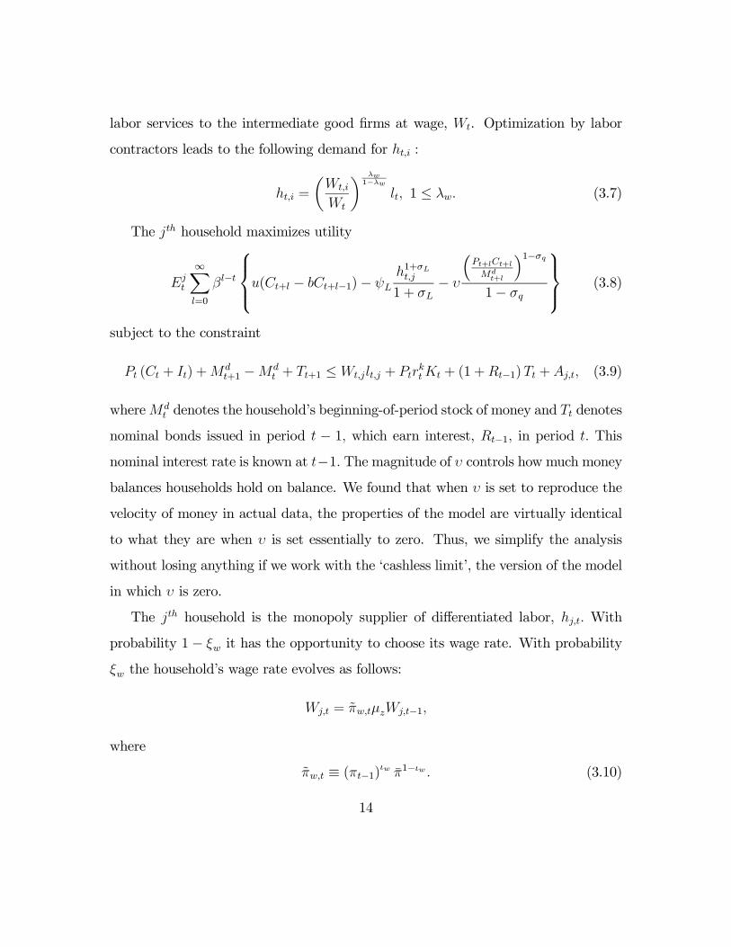
The solid line in Figure 3 displays the response of the economy to a signal in period
1 that technology will improve 1 percent in period 13. The starred lines represent
the response of the efficient allocations. The efficient allocations are obtained by
dropping the monetary policy rule, (3.12), and computing the best allocations that
are consistent with the remaining model equations.18 Note first how the equilibrium
responses overshoot the efficient responses to a signal shock. The percent responses in
output, consumption, investment and hours worked are roughly three times greater
18All calculations were done using the model-solution and simulation package, DYNARE. Al-
though the computation of the Ramsey-efficient allocations is conceptually straightforward, the
algebra required to derive the equations that characterize those allocations is laborious. In doing
the calculations we benefited greatly from the code prepared for Levin, Lopez-Salido (2004) and
Levin, Onatski, Williams, and Williams (2005), which automatically does the required algebra in a
format that can be input into DYNARE. It is perhaps worth stressing that monetary authority in
the efficient allocations does not have any information advantage over private agents.
16

in the equilibrium than they would be under an ideal monetary policy. Also, the
price of capital rises and then falls in the monetary equilibrium. The price of capital
corresponds to the price of equity in our model.19 The pattern of responses of the solid
line corresponds, qualitatively, to the pattern in a typical boom-bust episode.20 Since
the starred line represents the best that is feasible with monetary policy, according
to the analysis here most of the boom-bust episode reflects bad (in a welfare sense)
monetary policy.
We verified that the problem with monetary policy is that it focuses too narrowly
on inflation. If the coefficient on inflation in the monetary policy rule, (3.12), is
reduced to nearly unity, then the solid line and the starred lines essentially coincide.
Also, if the frictions in wage setting are removed by setting ξw = 0, then the starred
and solid lines also nearly coincide.
We found that if price frictions are eliminated, then the results are for the most
part unchanged. One difference is that inflation falls less quickly in the early phase
of the boom-bust.21 Regardless of sticky prices, however, everyone - the monetary
authority included - expects prices to fall when the positive technology shock actually
occurs. The anticipated monetary easing generated by this is enough to produce the
boom in the immediate aftermath of the signal. We conclude that it is the interaction
of sticky wages and a monetary policy too narrowly focused on inflation that accounts
19Note how the price of capital falls in the efficient allocations. For an extensive discussion of
this, see Christiano, Ilut, Motto and Rostagno (2007).20For what happens in boom-bust episodes, see, for example, Adalid and Detken (2006) and
Bordo and Wheelock (2007).21Presumably, in a more complete boom-bust scenario an actual rise in technology would accom-
pany the signal shock, and this would help place downward pressure on the price level in the wake
of the signal shock. In our analysis we do not allow for a rise in actual technology during the boom
in order to isolate the very large role played by expectations.
17

for the excessive volatility in allocations.
To understand the economics of the analysis, consider the dynamic behavior of
the real wage. In the equilibrium with the Taylor rule, the real wage falls, while
efficiency dictates that it rise. In effect, in the Taylor rule equilibrium the markets
receive a signal that the cost of labor is low, and this is part of the reason that the
economy expands so strongly. The ‘correct’ signal would be sent by a high real wage,
and this could be accomplished by allowing the price level to fall. However, in the
monetary policy regime governed by our Taylor rule, (3.12), this fall in the price level
is not permitted to occur: any threatened fall in the price level is met by a proactive
expansion in monetary policy. Not surprisingly, when we redo our analysis with a
Taylor rule in which longer-term inflation expectations appear, the problem is made
even worse.
As noted above, when Christiano, Ilut, Motto and Rostagno (2007) introduce
credit into the model they find that the solid line in the figure essentially drops to
the starred line. That is, allowing monetary policy to react to credit growth causes
the model response to a signal shock to virtually coincide with the efficient response.
4. Conclusion
We described two examples that illustrate in different ways how money and credit
may be useful in monetary policy. The first example shows how a commitment to
monitor money and control it directly in the event that it behaves erratically can
help anchor inflation expectations. The second example shows how a policy that
focuses too narrowly on inflation may inadvertently contribute to welfare-reducing
boom-bust cycles. According to the example, a policy of monetary tightening when
credit growth is strong can attenuate this unintended effect of too-narrow inflation
18

stabilization.
We emphasize that in our examples, the problem is not the stabilization of in-
flation expectations or inflation per se. The examples show that there can be trade-
offs between overly rigid inflation stabilization and the stabilization of asset prices
and output. The design of an efficient inflation stabilization program must balance
trade-offs, and to get these right one must get the structure of the economy right.
Fortunately, there has been great progress in recent years as increasingly sophisti-
cated macroeconomic models are developed and fit to data. In addition, there have
been substantial strides in the conceptual aspects of designing policies to stabilize
inflation.22 Each of our two examples perturbs the standard sticky price model in
directions that appear to be empirically plausible. The first example integrates fi-
nancial frictions in the supply side of the economy. The second example introduces
frictions in the setting of wages. These examples suggest to us that as the models
used for monetary policy analysis become more realistic, money and credit will come
to play a direct role in monetary policy.
22The recent work in ‘flexible inflation targeting’ (see Bernanke, 2003, for an informal discussion)
focuses on replacing (1.1) by the optimal policy. This requires taking a stand on the model of
the economy. When the economy is our benchmark economy, the monetary authority observes the
shocks striking the economy as they occur and the monetary authority’s objective is social welfare,
then optimal policy corresponds to the policy captured by the Ramsey policies exhibited in Figure 1.
Discussions of this approach appear in, among other places, Benigno andWoodford (2007), Gianonni
and Woodford (2005) and Svensson and Woodford (2005). This approach obviously requires that
the model economy be correctly specified and that the appropriate commitment technology exist
to resist the time inconsistency associated with optimal plans.
19
5. Appendix
In this appendix, we describe a perfect foresight version of the standard New Key-
nesian model.23 We show that when a working capital channel is added, then the
model displays the kind of multiplicity of equilibria discussed in the text. Although
the analysis is similar in spirit to the ones in BSU-CF-CR, the detailed example is
new. For this reason, we develop the example carefully.
We need only consider the perfect foresight version of the model because the
argument is based only on the properties of the model in a neighborhood of the
perfect foresight steady state. The first section below describes the agents in the
economy. Because the Taylor rule assumed in the equilibrium of our model involves
deviations from the optimal equilibrium, the second subsection presents a careful
discussion of optimality. We describe the best equilibrium that is supportable by
some feasible monetary and fiscal policy (i.e., the ‘Ramsey’ equilibrium). We also
describe a different concept, the best allocations that are feasible given only the
preferences and technology in the economy and ignoring the price-setting frictions.
Although the two concepts are different along a transition path, they coincide in
steady state. The third subsection below describes our Taylor rule, and presents our
basic result.
5.1. The Agents in the Economy
Households are assumed to have the following preferences:
∞Xt=0
βtµlogCt −
N1+ϕt
1 + ϕ
¶,
23See, for example, Woodford (2003a) and the references he cites.
20

where Nt denotes employment and Ct denotes consumption. We suppose that house-
holds participate in a labor market and in a bond market, leading to the following
efficiency conditions:
−ct = −rr + rt − ct+1 − πt+1,
ϕnt + ct = wt − pt,
where
rr ≡ − log β, ct ≡ logCt, rt ≡ logRt, wt = logWt, pt = logPt, πt ≡ pt − pt−1.
Here, Pt denotes the price of consumption goods, Wt denotes the nominal wage rate,
and Rt denotes the gross nominal rate of interest from t to t+ 1.
Final output is produced by a representative competitive producer with technol-
ogy:
Yt =
µZ 1
0
Yt (i)ε−1ε di
¶ εε−1
, ∞ > ε ≥ 1, (5.1)
where Yt (i) , is an intermediate good purchased at price Pt (i) , i ∈ [0, 1]. Final
output, Yt, is sold at price Pt and the representative final good firm takes Pt (i) and
Pt as given. Optimization by the representative final good producer implies:
Yt (i) = Yt
µPt (i)
Pt
¶−ε(5.2)
Substituting (5.2) into (5.1) and rearranging, we obtain:
Pt =
µZ 1
0
Pt (i)(1−ε) di
¶ 11−ε
. (5.3)
The ith intermediate good producer is a monopolist in the market for Yt (i) , but
interacts competitively in the labor market. The ith intermediate good producer’s
technology is given by:
Yt (i) = Nt (i) ,
21

and the producer’s marginal cost is:
(1− νt)Wt
Pt(1 + ψrt) ,
where νt is a potential subsidy received by the intermediate good firm from the
government. Any subsidy is assumed to be financed by a lump-sum tax to households.
The intermediate good producer faces Calvo-style frictions in the setting of prices.
A fraction, θ, of intermediate good firms cannot change price:
Pt (i) = Pt−1 (i− 1)
and the complementary fraction, 1− θ, sets price optimally:
Pt (i) = P̃t.
5.2. Ramsey (‘Natural’) Equilibrium
Given the nature of technology, the ideal allocation of labor occurs when it is spread
equally across the different intermediate good producers:
Nt (i) = Nt all i,
so that
Yt = Nt, yt = nt, (5.4)
where yt = log Yt. Efficiency in the total level of employment requires equating
the marginal cost of work in consumption units (the marginal rate of substitution
between work and leisure - MRSt) to the marginal benefit (the marginal product of
labor, MPL,t). In logs:log MRStz }| {ct + ϕnt =
log MPL,tz}|{0 (5.5)
22

Combine (5.4) and (5.5) and ct = yt to obtain:
yt (1 + ϕ) = 0
so that natural level of output and employment are:
y∗t = n∗t = 0. (5.6)
Under the ideal allocations, employment, consumption and output are all equal to
unity in each period.
The ideal allocations do not in general coincide with the Ramsey allocations: the
ones attainable by some feasible choice of monetary and fiscal policy. However, the
Ramsey allocations do converge to the ideal allocations in steady state.
We express the Ramsey equilibrium as the solution to a particular constrained
optimization problem. The pricing frictions and the technology imply, as shown in
Yun (1996, 2005):
Ct = Yt = p∗tNt, (5.7)
where p∗t is the following measure of price dispersion:
p∗t =
"Z 1
0
µPt(i)
Pt
¶−εdi
#−1,
where Pt is defined in (5.3). Note that p∗t = 1 when all intermediate goods prices are
the same. The law of motion for p∗t is obtained by combining the last equation with
the first order condition for firms that optimize their price. The resulting expression
is:
p∗t =
⎡⎣(1− θ)
Ã1− θ (πt)
ε−1
1− θ
! εε−1
+θπεtp∗t−1
⎤⎦−1 . (5.8)
23

Note that p∗t−1 = πt = 1 implies p∗t = 1. That is, if there was no price dispersion in
the previous period (i.e., p∗t−1 = 1) and there is no aggregate inflation in the current
period (i.e., πt = 1), then there is also no price dispersion in the current period.
To understand the intuition behind this result, recall that non-optimizers leave their
price unchanged. If in addition there is no aggregate inflation, then it must be that
optimizers also leave their price unchanged. If everyone leaves their price unchanged
and all intermediate firm prices were identical in the previous period, then it follows
that all intermediate good firm prices must be the same in the current period.
The first order necessary conditions associated with firms that optimize their
prices can be shown to be24:
1 +
µ1
πt+1
¶1−εβθFt+1 = Ft (5.9)
ε
ε− 1(1− νt)Wt (1 + ψrt)
Pt+ βθ
µ1
πt+1
¶−εKt+1 = Kt (5.10)
Ft
⎡⎢⎣1− θ³1πt
´1−ε1− θ
⎤⎥⎦1
1−ε
= Kt, (5.11)
where Ft and Kt represent auxiliary variables. Finally, we restate the household’s
inter- and intra- temporal Euler equations for convenience:
1
Ct=
β
Ct+1(1 + rt) /πt+1,
Wt
Pt= Nϕ
t Ct (5.12)
The allocations in a Ramsey equilibrium solve the Ramsey problem:
maxNt,Kt,νt,Ct,p∗tFt,πt,rt
∞Xt=0
βtµlogCt −
N1+ϕt
1 + ϕ
¶, (5.13)
subject to (5.7)-(5.12) and the given value of p∗−1. We now establish the following
proposition:24See, for example, Benigno and Woodford, (2004).
24

Proposition 5.1. The allocations in a Ramsey equilibrium are uniquely defined by
the following expressions:
πt = argmaxπt
p∗t =
" ¡p∗t−1
¢(ε−1)1− θ + θ
¡p∗t−1
¢(ε−1)# 1ε−1
, (5.14)
Nt = 1 (5.15)
p∗t =h1− θ + θ
¡p∗t−1
¢ε−1i 1ε−1
, (5.16)
limT→∞
PT = p∗−1P−1, (5.17)
1− νt =ε− 1
ε (1 + ψrt)(5.18)
1 + rt =1
β(5.19)
for t = 0, 1, 2, ..
According to (5.14) and (5.15), the only restrictions that bind on the solution
are the resource constraint, (5.7), and the law of motion for p∗t , (5.8). In particular,
πt, Nt and Ct may be chosen to solve (5.13) subject to (5.7) and (5.8), ignoring the
other restrictions on the Ramsey problem. The other restrictions may then be solved
for the remaining choice variables in the optimization problem, (5.13). The details
are reviewed in what follows.
Substitute out for Ct in (5.13) using (5.7) and then maximize the result with
respect to Nt and πt. The solution to this problem is characterized by (5.14) and
(5.15). Then, substitute out for πt from (5.14) into (5.8) to obtain (5.16). The
latter is a stable linear difference equation in (p∗t )ε−1 , with slope equal to θ. Because
0 < θ < 1, the difference equation is globally stable and has a unique fixed point at
p∗t = 1. Combining (5.16) and (5.14), we obtain:
πt =p∗t−1p∗t
. (5.20)
25

Note that although the resource allocation distortion, p∗t , is minimized according
to (5.14), it is not necessarily eliminated in each period. If p∗−1 6= 1 the resource
allocation distortion is eliminated gradually over time. Combining (5.20) with the
global stability of (5.16) we obtain (see Yun, 2005):
limT→∞
PT
P−1= lim
T→∞
p∗−1p∗T
= p∗−1.
This establishes (5.17).
Impose (5.7), (5.12) and (5.18) on (5.10) and divide by p∗t , to obtain:
1 + βθ
µ1
πt+1
¶1−εKt+1
p∗t+1=
Kt
p∗t, (5.21)
where (5.20) has been used. We use (5.21) to define Kt, so that (5.10) is satisfied.
Define
Ft =Kt
p∗t
Note
"1− θ (πt)
ε−1
1− θ
# 11−ε
=
⎡⎢⎣1− θ³p∗t−1p∗t
´ε−11− θ
⎤⎥⎦1
1−ε
=
⎡⎢⎢⎣1− θ(p∗t−1)
ε−1
1−θ+θ(p∗t−1)ε−1
1− θ
⎤⎥⎥⎦1
1−ε
=1h
1− θ + θ¡p∗t−1
¢ε−1i 11−ε
=1
p∗t,
so that (5.11) is satisfied. Note that given (5.21) and our definition of Ft, it follows
that (5.9) is satisfied. Finally, (5.19) is obtained by substituting (5.15), (5.20) and
(5.7) into (5.12). Since all the constraints on the problem, (5.13), are satisfied, the
proposition is established.
26

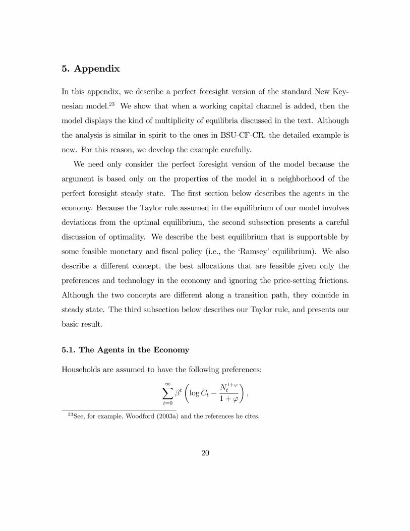
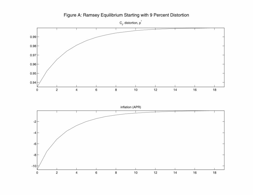
Four observations on the proposition are worth emphasizing. First, if p∗−1 6= 1
then πt = 1 for t = 0, 1, .. is not optimal. However, πt does optimally converge
to unity so that the allocations converge to what we call the ‘ideal’ allocations as-
ymptotically. To get a sense of how long the transition path is, consider the case
p∗−1 = 0.91. With this initial condition, output is 9 percent below potential, for any
given aggregate level of employment. The transition of inflation and the distortion
(or, equivalently, consumption) to the steady state is indicated in Figure A (we use
the following quarterly parameter values, θ = 0.75, ε = 5, ϕ = 1, β = 0.99). Note how
very far the inflation rate is from its steady state. The Ramsey level of consumption
also remains substantially below its steady state value. The example assumes that
the average duration of prices is one year (i.e., 1/(1− θ) = 4). With our parameteri-
zation, it takes about one year for the inflation rate and consumption to converge to
the Ramsey steady state.
A second observation worth emphasizing is that equation (5.18) implies the labor
subsidy on firms is chosen to completely eliminate the monopoly power distortion
and the distortion due to the financial friction. It is interesting that this distortion
is eliminated entirely, because the cross-sectoral distortion is not eliminated during
the transition (note that p∗t takes about three years to converge). The theory of the
second best might have led us to expect that if one distortion could not be eliminated,
then the other would not either.
Third, we note that the environment does not rationalize price level targeting.
Equation (5.17) implies that after a shock which drives the price level up in period
−1, average inflation is below steady state. This is because a shock to the aggregate
price level creates price dispersion, and this drives p∗−1 down. However, a shock in −1
which drives the aggregate price level down also drives p∗−1 down and so such a shock
is followed by a period of below steady state inflation too. Since price level targeting
27

requires that inflation be high after a shock that drives the price level down and low
after a shock that drives the price level up, it follows that price level targeting is
not a property of a Ramsey equilibrium. The environment does rationalize inflation
targeting, though it does not rationalize returning inflation to target immediately.
It instead rationalizes driving inflation to its target over time. Fourth, the fact that
(5.7) and (5.8) are the only restrictions that bind on the Ramsey problem indicates
that the Ramsey policy is time consistent. This is because neither (5.7) or (5.8)
incorporates expectations about the future. Thus, the Ramsey policy would be
implemented by a policymaker that has no ability to commit to future inflation.
The benchmark economy that we use is the steady state of the Ramsey equi-
librium. This corresponds to the ideal allocations defined at the beginning of this
section.
5.3. Equilibrium with Taylor Rule Monetary Policy
In our economy with a Taylor rule, we suppose that fiscal policy, vt, is set to ensure
that the steady state corresponds to the steady state of the Ramsey equilibrium:
1− vt =ε− 1
ε (1 + ψrr). (5.22)
Under the Taylor rule, the interest rate deviates from the Ramsey or natural rate
according to whether expected inflation is higher or lower than steady state inflation:
r̂t = τπt+1, r̂t ≡ rt − rr.
We repeat here the household intertemporal equilibrium condition in the Taylor rule
equilibrium:
yt = − [r̂t − πt+1] + yt+1.
28

The intertemporal equilibrium condition in steady state (either Ramsey or in the
economy with the Taylor rule) is:
y∗t = − [rr∗t − rr] + y∗t+1,
where y∗t is defined in (5.6) and rr∗t is the Ramsey (or, ‘natural’) rate of interest. We
deduce that rr∗t = rr. Subtracting the steady state intertemporal condition from the
one in the economy with the Taylor rule, we obtain the ‘New Keynesian IS equation’:
xt = − [r̂t − πt+1] + xt+1.
The log of (5.7) implies:
yt = log p∗t + nt.
In a sufficiently small neighborhood of steady state, log p∗t ≈ 0 (see Yun, 1996, 2005)
and we impose this from here on. This is appropriate because we are concerned with
the properties of equilibrium in a small neighborhood of steady state. The Calvo
reduced form inflation equation implies
πt = βπt+1 + κ× cmct, κ =(1− θ) (1− βθ)
θ,
where cmct denotes the log deviation of real marginal cost in the Taylor rule equilib-
rium from its log steady state value, mc∗:
mc∗ = log (1− ν) + logWt
Pt+ log (1 + ψrr)
= logε− 1ε
,
using (5.16), the household’s static Euler equation and the fact that output and
employment are unity in steady state. Then,
cmct = log (1− νt) + logWt
Pt+ log (1 + ψrt)−mc∗t
= log (1− ν) + ϕnt + ct + ψrt − log (1− ν)− ψrr
= (ϕ+ 1)xt + ψr̂t,
29

using the household’s static Euler equation and (5.7). Also, we have used the ap-
proximation,
log (1 + ψrt) ' ψrt.
Substituting this into the Phillips curve, we obtain:
πt = βπt+1 + κ (ϕ+ 1)xt + κψr̂t.
Collecting the equilibrium conditions, we obtain:
πt = βπt+1 + κ (ϕ+ 1)xt + κψr̂t ‘Phillips curve’
xt = − [r̂t − πt+1] + xt+1 ‘IS curve’
r̂t = τπt+1 ‘Taylor rule’.
5.4. Determinacy Properties of the Nonstochastic Steady State
Using the monetary policy rule to substitute out for r̂t :
xt + σ (τ − 1)πt+1 − xt+1 = 0
πt − λxt − (β + γτ)πt+1 = 0,
where σ is the intertemporal elasticity of substitution (assumed unity in the previous
derivation). Also,
λ = κ (ϕ+ 1)
γ = κψ.
Expressed in matrix form, the system is:⎡⎣ σ (τ − 1) −1
− (β + γτ) 0
⎤⎦⎛⎝ πt+1
xt+1
⎞⎠+⎡⎣ 0 1
1 −λ
⎤⎦⎛⎝ πt
xt
⎞⎠ =
⎛⎝ 0
0
⎞⎠ ,
30

for t = 0, 1, 2, ... , or, after inverting:⎛⎝ πt+1
xt+1
⎞⎠ = A
⎛⎝ πt
xt
⎞⎠ , (5.23)
where
A =1
β + τγ
⎡⎣ 1 −λa b
⎤⎦ , a = σ (τ − 1) , b = β + τγ − λa.
Note that the eigenvalues of A solve:
μ =1
2(b+ 1)± 1
2
√b2 − 4aλ− 2b+ 1.
Local uniqueness of the steady state equilibrium, xt = 0 = πt, requires that both
eigenvalues of A exceed unity in absolute value. To see why, note first that both
xt and πt are endogenous variables whose values are determined at time t (they are
period t ‘jump’ variables). If one or both eigenvalues of A were less than unity in
absolute value, one could set some combination of x0 and π0 different from zero,
and the solution to (5.23) describes a path that eventually takes the system back
to steady state (i.e., (xt, πt) → 0, as t → ∞). Because there is an uncountable
number of such combinations, (x0, π0), each of which follows a path back to steady
state and each such path satisfies the equilibrium conditions, it follows that there is
a multiplicity of equilibria. Consider, for example, the parameter values:
θ = 0.75, κ = 0.085, τ = 1.5, σ = 1, ϕ = 1, ψ = 1, β = 0.99, γ = κ.
These parameter values are standard. They imply that the average time between
price changes is one year (see θ); the coefficient on expected inflation, τ , represents
an aggressive reaction to inflation; households have log utility (see σ); the (Frisch)
labor supply elasticity is unity (see ϕ); and the discount rate is 4 percent per year
(see β). We set ψ = 1, so that intermediate good firms are assumed to have to
31

finance 100% of their variable input costs (i.e., labor) in advance. We found that
in this example, the smallest (in absolute value) root of A is 0.94. So, we have a
multiplicity of equilibria, as in the discussion of the text. We found that the smallest
root of A is less than unity for all ψ ≥ 0.08. For ψ smaller than this, we reproduce the
standard result that both eigenvalues of A are greater than unity. This is consistent
with the intuition described in the body of the paper.
To assess the empirical plausibility of the range of values of ψ that produce multi-
plicity of equilibrium, we examined the Quarterly Financial Report for Manufactur-
ing, Mining, and Trade Corporations: 2006, Quarter 1, issued June 2006 (US Bureau
of the Census, available online at http://www.census.gov/prod/2006pubs/qfr06q1.pdf).
According to Table 1.0, page 2, sales in 2006Q1 were S =$1.4 trillion. According
to Table 1.1, page 4, short term liabilities (bank loans and commercial paper with
maturity less than one year, plus trade credit, plus other current liabilities) totaled
L =$1.3 trillion. If we take S/L as a (very) crude estimate of ψ, we conclude that
the range of values of ψ that generate multiple equilibria is empirically reasonable.
32

References
[1] Adalid, Ramon, and Carsten Detken, 2006, ‘Excessive Liquidity and Asset Price
Boom/Bust Cycles,’ manuscript, European Central Bank.
[2] Barro, Robert 1977, ‘Long-Term Contracting, Sticky Prices and Monetary Pol-
icy,’ Journal of Monetary Economics 3(3), 305-316.
[3] Barth, Marvin, III and Valerie A. Ramey, 2002, The Cost Channel of Monetary
Transmission, in Bernanke, Ben and Kenneth Rogoff, eds., NBER Macroeco-
nomics Annual 2001, vol. 16, Cambridge and London: MIT Press, 199-240.
[4] Beaudry, Paul and Franck Portier, 2004, “An Exploration into Pigou’s Theory
of Cycles,” Journal of Monetary Economics, September, 51(6): 1183-1216.
[5] Beaudry, Paul and Franck Portier, 2006, ‘Stock Prices, News, and Economic
Fluctuations,’ American Economic Review, September, 96(4): 1293-1307.
[6] Benhabib, Jess, Stephanie Schmitt-Grohe, Martin Uribe, 2001, “Monetary Pol-
icy and Multiple Equilibria,”American Economic Review, March, 91(1): 167-86.
[7] Benhabib, Jess, Stephanie Schmitt-Grohe, Martin Uribe, 2002a, ‘Chaotic
Interest-Rate Rules,’ American Economic Review, May, 92(2): 72-78.
[8] Benhabib, Jess, Stephanie Schmitt-Grohe, Martin Uribe, 2002b, “Avoiding Liq-
uidity Traps,” Journal of Political Economy, June, 110(3): 535-63.
[9] Benigno, Pierpaolo, and Michael Woodford, 2004, ‘Optimal Stabilization Policy
when Wages and Prices are Sticky: the Case of a Distorted Steady State,’
National Bureau of Economic Research working paper 10839.
33

[10] Benigno, Pierpaolo, and Michael Woodford, 2007, “Linear-Quadratic Approx-
imation of Optimal Policy Problems,” Manuscript, Columbia University, Sep-
tember 22.
[11] Bernanke, Ben, 2003, Remarks at the Annual Washington Policy Conference of
the National Association of Business Economists, Washington, D.C., March 25.
[12] Bernanke, Ben S., T. Laubach, F. S. Mishkin, and A. S. Posen, 1999, Infla-
tion Targeting: Lessons from the International Experience. Princeton University
Press.
[13] Bordo, Michael and David C.Wheelock, 2007, ‘Stock Market Booms and Mone-
tary Policy in the Twentieth Century,’ Federal Reserve Bank of St. Louis Review,
March/April, 89(2), pp. 91-122.
[14] Borio, Claudio and Philip Low, 2002, “Asset Prices, Financial and Monetary
Stability: Exploring the Nexus,” BIS Working Paper no. 114.
[15] Carlstrom, Charles T. and Timothy S. Fuerst, 2002, Taylor Rules in a Model
that Satisfies the Natural-Rate Hypothesis,” American Economic Review, May,
92(2): 79-84
[16] Carlstrom, Charles T. and Timothy S. Fuerst, 2005, “Investment and Interest
Rate Policy: A Discrete Time Analysis,” Journal of Economic Theory, July,
123(1): 4-20.
[17] Cecchetti, Stephen, and M. Ehrmann, 2002, ‘Does Inflation Targeting Increase
Output Volatility? An International Comparison of Policymakers’ Preferences
and Outcomes’ in Norman Loayza and Klaus Schmidt-Hebbel (editors), Mon-
etary Policy: Rules and Transmission Mechanisms, Proceedings of the Fourth
34

Annual Conference of the Central Bank of Chile, Santiago, Chile: Central Bank
of Chile, pg. 247-274.
[18] Christiano, L. J., M. Eichenbaum, and C. Evans, 1996, “The Effects of Monetary
Policy Shocks: Evidence from the Flow of Funds,” Review of Economics and
Statistics, 78, 16-34.
[19] Christiano, L. J., M. Eichenbaum, M., and C. Evans, 1999, “Monetary Pol-
icy Shocks: What have we Learned and to what End?” in J. B. Taylor, and
M.Woodford, ed., Handbook of Macroeconomics, Elsevier Science, North Hol-
land.
[20] Christiano, L. J., M. Eichenbaum, M., and C. Evans, 2005, “Nominal Rigidities
and the Dynamic Effects of a Shock to Monetary Policy,” Journal of Political
Economy, February, 113(1): 1-45.
[21] Christiano, Lawrence, Cosmin Ilut, Roberto Motto and Massimo Rostagno,
2007, ‘Monetary Policy and Stock Market Boom-Bust Cycles,’ manuscript avail-
able at http://faculty.wcas.northwestern.edu/~lchrist/research.htm.
[22] Christiano, Lawrence andMassimo Rostagno, 2001, “Money GrowthMonitoring
and the Taylor Rule,” National Bureau of Economic Research Working paper
number 8539.
[23] Eichengreen, Barry and Kris J Mitchener, 2004, ‘The Great Depression as a
Credit Boom Gone Wrong,’ in Field, Alexander J., ed. Research in economic
history. Volume 22. Coedited by Gregory Clark and William A. Sundstrom.
Oxford; Amsterdam and San Diego: Elsevier, JAI, 183-237
35

[24] Erceg, Christopher, Dale Henderson, and Andrew Levin, 2000, ‘Optimal Mon-
etary Policy with Staggered Wage and Price Contracts,’ Journal of Monetary
Economics, 46, 281-313.
[25] Gertler, Mark, Luca Sala and Antonella Trigari, 2007, ‘An Estimated Monetary
DSGE Model with Unemployment and Staggered Nominal Wage Bargaining,’
manuscript, New York University.
[26] Giannoni, Marc P., and Michael Woodford, 2005, ‘Optimal Inflation Target-
ing Rules,’ in Bernanke, Ben S., and Michael Woodford, eds., The Inflation-
Targeting Debate, University of Chicago Press, 19-83.
[27] Jaimovic, Nir, and Sergio Rebelo, 2006, ‘Do News Shocks Drive the Business
Cycle?,’ Northwestern University.
[28] Levin, A., Lopez-Salido, J.D., 2004. "Optimal Monetary Policy with Endoge-
nous Capital Accumulation", manuscript, Federal Reserve Board.
[29] Levin, A., Onatski, A., Williams, J., Williams, N., 2005, "Monetary Policy under
Uncertainty in Microfounded Macroeconometric Models," in, NBER Macroeco-
nomics Annual 2005, Gertler, M., Rogoff, K., eds. Cambridge, MA: MIT Press.
[30] Lucca, David, 2006, Essays in Investment and Macroeconomics, Doctoral Dis-
sertation, Northwestern University.
[31] Matsuyama, Kiminori, 1984, ‘A Learning Effect Model of Investment: An Al-
ternative Interpretation of Tobin’s Q’, manuscript, Northwestern University.
[32] McCallum, Bennett, 2001, ‘Monetary Policy Analysis in Models Without
Money,’ Federal Reserve Bank of St. Louis Review 83(4), 145-160.
36

[33] Midrigan, Virgiliu, 2005, ‘Menu Costs, Multi-Product Firms and Aggregate
Fluctuations,’ manuscript.
[34] Nakamura, Emi, and Jón Steinsson, 2006, ‘Five Facts About Prices: A Reeval-
uation of Menu Cost Models,’ manuscript, Harvard.
[35] Smets, Frank and Raf Wouters, 2003, “An Estimated Dynamic Stochastic Gen-
eral Equilibrium Model of the Euro Area,” Journal of the European Economic
Association, September, 1(5): 1123-75.
[36] Smets, Frank and Raf Wouters, 2007, “Shocks and Frictions in US Business
Cycles: A Bayesian DSGE Approach,” American Economic Review, Vol. 97,
No. 3, June.
[37] Svensson, Lars E.O., 1997, ‘Inflation Forecast Targeting: Implementing and
Monitoring Inflation Targets,’ European Economic Review, 41, pp. 1111-1146.
[38] Svensson, Lars E.O. and Robert J. Tetlow, 2005, “Optimal Policy Projections”,
International Journal of Central Banking, vol. 1 n. 3, December.
[39] Svensson, Lars E.O. and Michael Woodford, 2005, “Implementing Optimal Pol-
icy through Inflation-Forecast Targeting,” in Bernanke, Ben S., and Michael
Woodford, eds., The Inflation-Targeting Debate, University of Chicago Press,
19-83.
[40] Woodford, Michael, 1998, ‘Doing Without Money: Controlling Inflation in a
Post-Monetary World,’ keynote address at the annual meeting of the Society for
Economic Dynamics and Control in Mexico City, June 1996, Review of Economic
Dynamics 1: 173-219.
37

[41] Woodford, Micael, 2003a, Interest and Prices: Foundations of a Theory of Mon-
etary Policy, Princeton University Press.
[42] Woodford, Micael, 2003b, “Optimal Interest-Rate Smoothing,” Review of Eco-
nomic Studies 70: 861-886.
[43] Yun, Tack, 1996, ‘Nominal Price Rigidity, Money Supply Endogeneity, and Busi-
ness Cycles,’ Journal of Monetary Economics, 37(2): 345 - 370.
[44] Yun, Tack, 2005, ‘Optimal Monetary Policy with Relative Price Distortions,’
The American Economic Review, March.
38

RFigure 1a
LM’
LM
IS(πe’)
IS(πe)
yy2 y1
LM( )
Phillips curveπ1
π
π2
y2 y1 yFigure 1b

RFigure 2a
LM’
LM
IS(πe’)
IS(πe)
yy2 y1
LM( )
Phillips curveπ2
π1
π
Higher πe confirmed and likely to persist
y2 y1 yFigure 2b

5 10 15 200
0.2
0.4
0.6
0.8
1
outputpe
rcen
t dev
iatio
n fr
om s
s
5 10 15 20
0
0.2
0.4
0.6
consumption
perc
ent d
evia
tion
from
ss
5 10 15 202
4
6
8
10
12
14net real rate of interest
annu
aliz
ed, p
erce
nt
5 10 15 200
0.5
1
hours worked
perc
ent d
evia
tion
from
ss
5 10 15 200
0.5
1
1.5
investment
perc
ent d
evia
tion
from
ss
5 10 15 204
6
8
10
12
14
Ann
ualiz
ed, p
erce
nt
net nominal rate of interest
5 10 15 20-1
-0.5
0
perc
ent d
evia
tion
from
ss
price of capital
Figure 3: Benchmark Monetary Model and Associated Ramsey-efficient Allocations
5 10 15 20
-0.2
-0.1
0
0.1
0.2
perc
ent d
evia
tion
from
ss
real wage
Ramsey Allocations of Simple Monetary ModelSimple Monetary Model
0 2 4 6 8 10 12 14 16 18
0.94
0.95
0.96
0.97
0.98
0.99
Ct, distortion, p*
Figure A: Ramsey Equilibrium Starting with 9 Percent Distortion
0 2 4 6 8 10 12 14 16 18
-10
-8
-6
-4
-2
inflation (APR)