TWO MATHEMATICAL MODELS FOR PERFORMANCE …lucian/en/revueroumain05.pdf · TWO MATHEMATICAL MODELS FOR PERFORMANCE EVALUATION OF LEAKY-BUCKET ALGORITHM LUCIAN IOAN, GRAZZIELA NICULESCU

TWO MATHEMATICAL MODELS FOR PERFORMANCE EVALUATION OF LEAKY-BUCKET ALGORITHM

LUCIAN IOAN, GRAZZIELA NICULESCU

Key words: B-ISDN, ATM, cell, congestion/access control, Leaky-Bucket, simulation, traffic negotiation.

Abstract: The multimedia services development needs the implementation of the special networks, which must be able to serve in the unitary way the heterogeneous flows, whose debits vary into a large scale. The random character of the debits impose the conception of new algorithms for traffic control and for general network management. The main purpose of this paper is the development of two mathematical models of an algorithm, named ’’Leaky-Bucket mechanism’’ used for the parameter usage of connection control.

1. INTRODUCTION

The broadband networks, with the informational debits more than 45Mb/s, remove some troubles of the classical networks, such as: the service dependency, inflexibility to the traffic characteristics changes and the global inefficiently usage of the resources. The Broadband Integrated Services Digital Network, B-ISDN assures a unique architecture for many and various services, a good protection against the traffic fluctuations and in the same time an optimal utilization of all resources. These facilities are possible thanks to the new technique, generally named Asynchronous Transfer Mode, ATM. This technique realizes the fast packed switch, allowing the systems to operate at a very high speed and to transport of all traffic flows indifferent which are theirs characteristics concerning the bit rate and the requirements for quality of real time service.

To accomplish this task the network must monitoring and controlling the traffic offered by sources to prevent accidental or intentional violations of the negotiated parameters that can affect QoS of already established connections. For this purpose on mention the Leaky-Bucket device that will be analyzed in the following.

Lucian Ioan, Grazziela Niculescu

2

2. LEAKY-BUCKET MECHANISM

In the ATM networks the cell flows between the sources and the destinations use the same intermediary paths during the whole communication period. The flows concerning the different connections are statistical multiplexed on the ATM links. The dynamic allocation of the transmission channel imposes a traffic control to maintaining the quality of service. Otherwise the loss probability of cells or delay can grow above the accepted customers' limits. But during the connection one source can violate the negotiated values. The special mechanisms for the traffic control and its maintaining in the negotiated limits act in the ATM networks. The most frequently used is Leaky-Bucket mechanism (LB).

Offered traffic Served traffic

Credits generator Counter +–

Fig.1 – Schematic of the LB mechanism

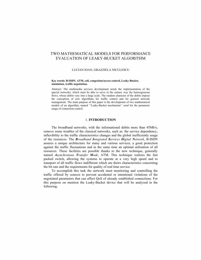
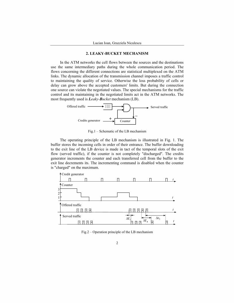
The operating principle of the LB mechanism is illustrated in Fig. 1. The buffer stores the incoming cells in order of their entrance. The buffer downloading to the exit line of the LB device is made in tact of the temporal slots of the exit flow (served traffic), if the counter is not completely "discharged". The credits generator increments the counter and each transferred cell from the buffer to the exit line decrements its. The incrementing command is disabled when the counter is "charged" on the maximum.

Counter 3 2 1

Credit generator t

Offered traffic

Served traffic ∆t 1 ∆t 4

5t∆

t

t

t

1 2 3 4

1 2 3 4

1 2 3 4 5

1 2 3 4 5

Fig.2 – Operation principle of the LB mechanism

Mathematical models for Leaky-Bucket mechanism

3

The Fig. 2 contains four graphics. In the first of them is plotted the sequence of increment pulses send by the credit generator to the counter. The third image represents a possible arrival pattern of cells in the input line. These two sequences control the state of the counter. One particular state transition is plotted in the second graphic where we assume that the highest value stored in the counter is 3 and, at the moment when we start the graphic representation, the counter is in its maximum state.

The last graphic shows the succession of cells on the output line of the LB mechanism. In this example, the first burst of cells generated on the output line is identical with that one received, but in the second case, the cells no. 4 and no. 5 are delayed until credits are received by the counter.

The maximum value stored in the counter represents the maximum number of the successive temporal slots in which the device can transfer one incoming burst. The arrival rate of the credits is established at the negotiated value of the average debit of the incoming traffic. As is shown in the Fig. 2, the bursts that exceed the negotiated limits are disturbed by variable delays from one cell to other. If this situation becomes currently, then the delays will be unacceptable. In this case it is preferably to lose cells; the buffer capacity determines the losses percentage.

3. MATHEMATICAL MODELS OF THE GENERAL LB MECHANISM

3.1 FUNDAMENTAL CONSIDERATIONS

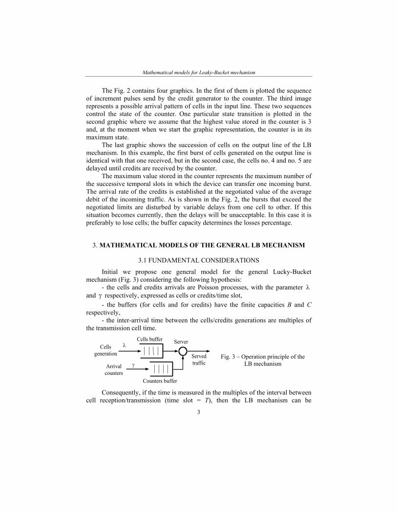
Initial we propose one general model for the general Lucky-Bucket mechanism (Fig. 3) considering the following hypothesis:

- the cells and credits arrivals are Poisson processes, with the parameter λ and γ respectively, expressed as cells or credits/time slot,

- the buffers (for cells and for credits) have the finite capacities B and C respectively,

- the inter-arrival time between the cells/credits generations are multiples of the transmission cell time.

λ

γ Served traffic

Counters buffer

Cells buffer

Arrival counters

Server Cells

generation

Fig. 3 – Operation principle of the LB mechanism

Consequently, if the time is measured in the multiples of the interval between cell reception/transmission (time slot = T), then the LB mechanism can be


4

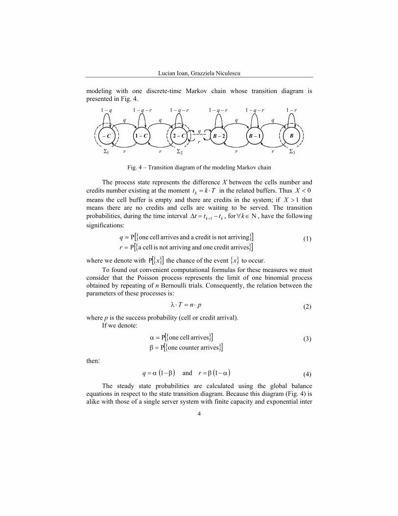
modeling with one discrete-time Markov chain whose transition diagram is presented in Fig. 4.

1 – q – r

1 – C – C 2 – C

1 – q

Σ1

q

r r

q

1 – q – r 1 – q – r

q

r B – 2

1 – q – r 1 – r

r

q

r

q

B – 1 B

Σ2 Σ3

Fig. 4 – Transition diagram of the modeling Markov chain

The process state represents the difference X between the cells number and credits number existing at the moment Tktk ⋅= in the related buffers. Thus 0<X means the cell buffer is empty and there are credits in the system; if 1>X that means there are no credits and cells are waiting to be served. The transition probabilities, during the time interval kk ttt −=∆ +1 , for Ν∈∀k , have the following significations:

{ }[ ]{ }[ ]arrivescredit one and arrivingnot is cell aP

arrivingnot iscredit a and arrives cell oneP==

rq

(1)

where we denote with { }[ ]xP the chance of the event { }x to occur. To found out convenient computational formulas for these measures we must

consider that the Poisson process represents the limit of one binomial process obtained by repeating of n Bernoulli trials. Consequently, the relation between the parameters of these processes is:

pnT ⋅=⋅λ (2)

where p is the success probability (cell or credit arrival). If we denote:

{ }[ ]{ }[ ]arrivescounter oneP

arrives cell oneP=β=α

(3)

then: ( ) ( )α−β=β−α= 1and 1 rq (4)

The steady state probabilities are calculated using the global balance equations in respect to the state transition diagram. Because this diagram (Fig. 4) is alike with those of a single server system with finite capacity and exponential inter


5

arrival and service time, we can write the following results:

[ ]( )

=ρ++

≠ρρρ−

ρ−=−==

−

++

1for ,1

1for ,1

1P

1

1

CBCjXp

jCB

j and CBj += ,0 (5)

where:

( )( )

( )( )T

Trq

λ−γγ−λ

=α−ββ−α

==ρ11

11 (6)

The ratio ρ can be considered as a parameter usage indicator because, if it is more than one, then negotiated parameters are exceeded and if it is less than one, then the negotiated values are respected. To obtain a valid value for the ratio ρ , the parameters involved in its computational formula must respect the following constraints:

T10 <λ< and T10 ≤γ< .

The ratio T1 means one cell or credit by time slot, being the maximum possible value for these both rates λ and γ .

3.2 PERFORMANCE EVALUATION

The computational formulas of the performance indicators that characterize our first proposed model are the followings:

- average number of memorized cells in buffer:

[ ] ( )( ) ( ) ( )

( )( )( )

( )

=ρ++

+

≠ρρ−ρ−

ρρ−+−ρρ−

=⋅−=++

++++

+

=∑

1for ,12

1

1for ,11

111

E1

11!

CBBB

B

pCjNCB

CBCB

CB

Cjj

(7)

- blocking probability of cells, which represents the ratio between the rate of rejected cells rλ and the cell generation rate λ :

( )

( )

=ρ++

≠ρρ−

ρρ−==

λλ

=−

++

+

+

1for,1

1for,11

1

1

CBpp CB

CB

CBr

b (8)

- guaranteed output rate (service rate) of the system:


6

( )

=ρ++

+λ

≠ρρ−ρ−

λ=−λ=λ

++

+

+

1for ,1

1for ,11

11

CBCB

pCB

CB

CBg

(9)

- mean delay (average of the waiting time) in the cells buffer (calculated with respect to the Little formula [ ] [ ] gN λ=τ EE ):

[ ]( )[ ]

( ) ( )( )( )

=ρ+λ+

≠ρρ−ρ−λ

ρρ+ρ+−

=τ+

++

1for,2

1

1for,11

11

E

11

CBBB

BBCB

CBB

(10)

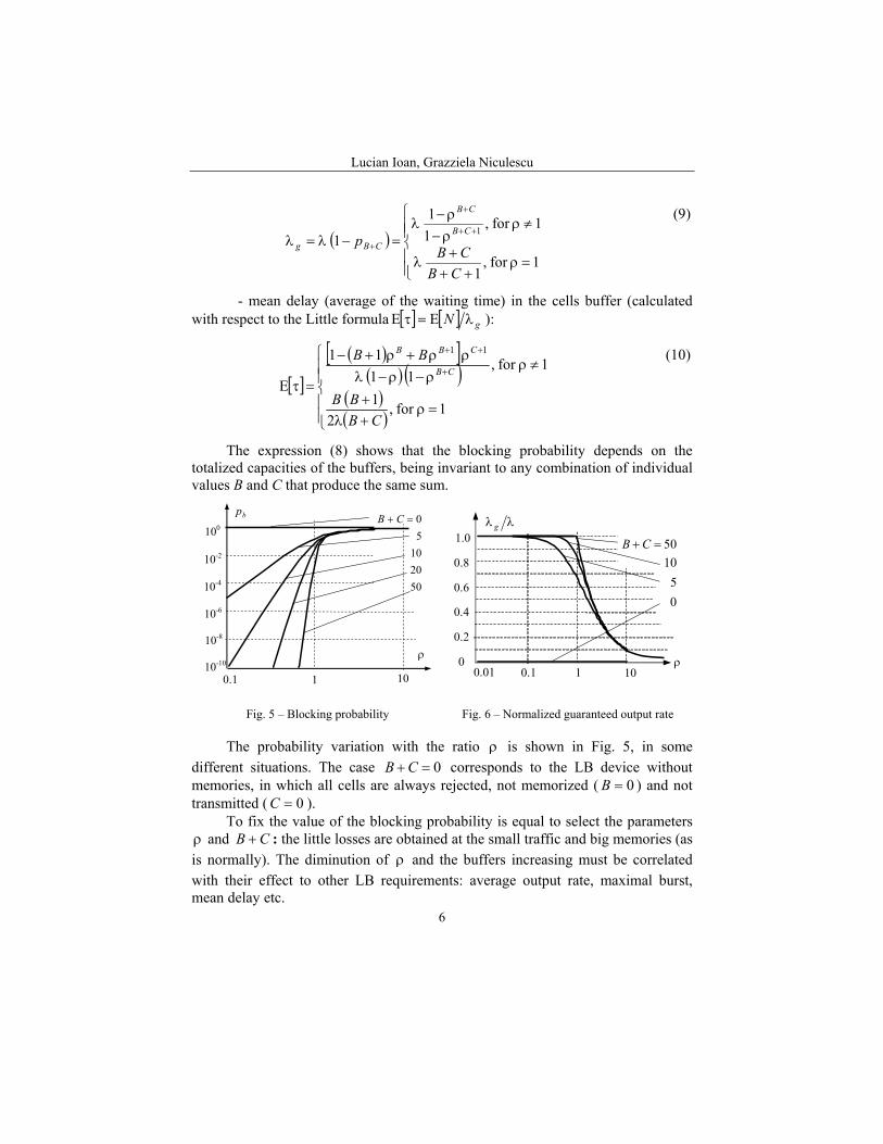
The expression (8) shows that the blocking probability depends on the totalized capacities of the buffers, being invariant to any combination of individual values B and C that produce the same sum.

502010

50=+ CB

ρ

bp

1 100.1 10-10

10-8

10-6

10-2

100

10-4

10 10.10.01ρ

1.0

0.8

0.6

0.4

0.2

0

λλ g

50=+ CB

05

10

Fig. 5 – Blocking probability Fig. 6 – Normalized guaranteed output rate

The probability variation with the ratio ρ is shown in Fig. 5, in some different situations. The case 0=+ CB corresponds to the LB device without memories, in which all cells are always rejected, not memorized ( 0=B ) and not transmitted ( 0=C ).

To fix the value of the blocking probability is equal to select the parameters ρ and CB + : the little losses are obtained at the small traffic and big memories (as is normally). The diminution of ρ and the buffers increasing must be correlated with their effect to other LB requirements: average output rate, maximal burst, mean delay etc.


7

The average output rate is strongly linked to the blocking probability, its variation with the ρ parameter and the sum CB + being plotted in Fig. 6. As it was expected, a modification of the traffic and buffer capacity, that gives a smaller value for the blocking probability, leads to an upper output rate that approaches the input rate value.

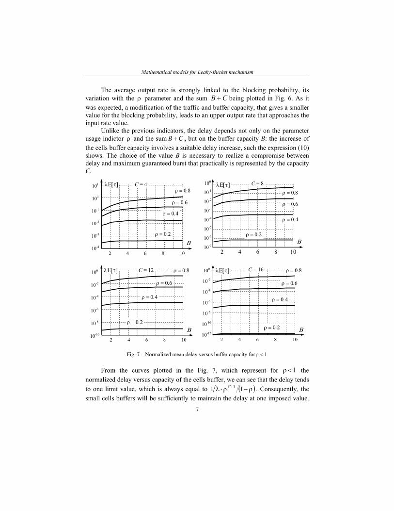
Unlike the previous indicators, the delay depends not only on the parameter usage indictor ρ and the sum CB + , but on the buffer capacity B: the increase of the cells buffer capacity involves a suitable delay increase, such the expression (10) shows. The choice of the value B is necessary to realize a compromise between delay and maximum guaranteed burst that practically is represented by the capacity C.

10-4

10

Β

6 8

λΕ[τ]

4 2

10-3

10-2

10-1

100

101

ρ = 0.8

ρ = 0.2

ρ = 0.4

ρ = 0.6

C = 4

10-7

10-6

10-5

10-4

10-3

100

Β

λΕ[τ] C = 8

ρ = 0.2

ρ = 0.8

ρ = 0.4

ρ = 0.6

2 4 6 8 10

10-2

10-1

10-6

10-4

10-2

10-10

100

10-8

Β

106 84 2

ρ = 0.8

ρ = 0.2

ρ = 0.4

ρ = 0.6

C = 12 λΕ[τ]

10-6

10-4

10-2

10-12

100

10-8

Β

10 6 8 42

ρ = 0.8

ρ = 0.2

ρ = 0.4

ρ = 0.6

C = 16λΕ[τ]

10-10

Fig. 7 – Normalized mean delay versus buffer capacity for 1<ρ

From the curves plotted in the Fig. 7, which represent for 1<ρ the normalized delay versus capacity of the cells buffer, we can see that the delay tends to one limit value, which is always equal to ( )ρ−ρ⋅λ + 11 1C . Consequently, the small cells buffers will be sufficiently to maintain the delay at one imposed value.


8

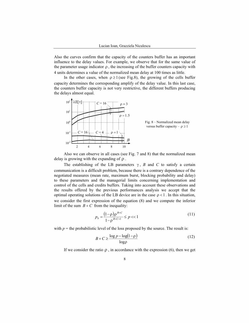
Also the curves confirm that the capacity of the counters buffer has an important influence to the delay values. For example, we observe that for the same value of the parameter usage indicator ρ , the increasing of the buffer counters capacity with 4 units determines a value of the normalized mean delay at 100 times as little.

In the other cases, when 1≥ρ (see Fig.8), the growing of the cells buffer capacity determines the corresponding amplify of the delay value. In this last case, the counters buffer capacity is not very restrictive, the different buffers producing the delays almost equal.

ρ = 1

ρ = 1.5

ρ = 3 C = 16

C = 16 C = 4

10-2

10-1

100

101

102

10

Β

6 84 2

λΕ[τ]

Fig. 8 – Normalized mean delay versus buffer capacity – 1≥ρ

Also we can observe in all cases (see Fig. 7 and 8) that the normalized mean delay is growing with the expanding of ρ .

The establishing of the LB parameters γ , B and C to satisfy a certain communication is a difficult problem, because there is a contrary dependence of the negotiated measures (mean rate, maximum burst, blocking probability and delay) to these parameters and the managerial limits concerning implementation and control of the cells and credits buffers. Taking into account these observations and the results offered by the previous performances analysis we accept that the optimal operating solutions of the LB device are in the case 1<ρ . In this situation, we consider the first expression of the equation (8) and we compute the inferior limit of the sum CB + from the inequality:

( ) 111

1 <<≤ρ−

ρρ−= ++

+

pp CB

CB

b (11)

with p = the probabilistic level of the loss proposed by the source. The result is:

( )ρ

ρ−−≥+

log1loglog pCB (12)

If we consider the ratio ρ , in accordance with the expression (6), then we get


9

the generation credits rate expressed in the following form:

( )ρ−λ+ρλ

=λ+λρ−ρ

λ=γ

1TTT (13)

Waiting time and the maximum burst are interdependent: the burst amplification (and consequently of the capacity C) involves the delay diminution (that also depends on capacity B) and vice versa. For this reason the both values are chosen in respect to the delay for each service.

The LB mechanism must regulate the received flows from the sources in the negotiated limits. The deviations from these limits are penalized by the quality of service diminution. So, if the source keep the average debit ( ρ is not exceeded), but it generates longer bursts that exceed the capacity C, or contrary the debit is increased, then LB device reacts introducing supplementary losses and delays.

3.3 OPERATING ALGORITHMS (ORDINARY FORMS)

A) The negotiated phase of the traffic contract between source and network may be processed by the following algorithm:

- choice of the parameters: blocking probability bp , cells arriving rate λ , transmission speed [ ]bpsv , mean delay and maximum burst interval vt ;

- computing of the cell duration: [ ] [ ]bps/b853 vT ⋅= . The cell duration must be less than λ1 . In this case the event:

{inter arrival time is less than sell duration} have very rare occurrence and the hypothesis "cells arrivals respect a Poisson process" is right.

- computing the sum CBS += in respect to the relation (12); - computing the credits buffer, in respect to the top debit) and after the cells

buffer: TtC v /= and CSB −= ; - computing the credits generation rate γ corresponding to the relation (13). B) The verifying phase, when the LB device controls if the negotiated values

are respected, especially the source emission rate, can use the following control algorithm:

- consider the fixed parameters: TCB ,,,γ ; - select the variable parameter λ ; - compute the parameter usage indicator ρ from the expression (6); - measure the QoS degradation degree by computing the blocking

probability bp following the relation (8).


10

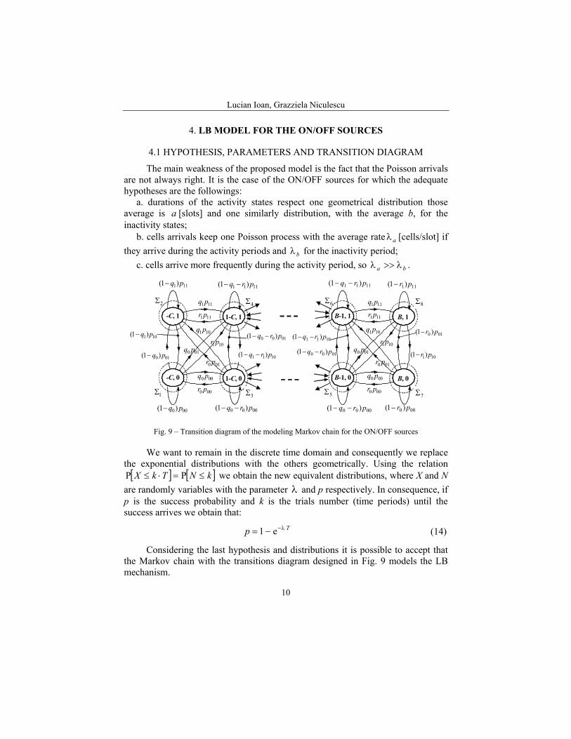
4. LB MODEL FOR THE ON/OFF SOURCES

4.1 HYPOTHESIS, PARAMETERS AND TRANSITION DIAGRAM

The main weakness of the proposed model is the fact that the Poisson arrivals are not always right. It is the case of the ON/OFF sources for which the adequate hypotheses are the followings:

a. durations of the activity states respect one geometrical distribution those average is a [slots] and one similarly distribution, with the average b, for the inactivity states;

b. cells arrivals keep one Poisson process with the average rate aλ [cells/slot] if they arrive during the activity periods and bλ for the inactivity period;

c. cells arrive more frequently during the activity period, so ba λ>>λ .

2Σ

-C, 1

111)1( pq−

111pr 111pq

1-C, 1

4Σ

1111 )1( prq −−

1Σ

-C, 0

000 pr 000 pq 1-C, 0

3Σ

010)1( pq−

101)1( pq−

000)1( pq− 0000 )1( prq −−

101pq

1011 )1( prq −−

0100 )1( prq −−101 pr

010 pq

010 pr

6Σ

B-1, 1

1111 )1( prq −−

111pr111pq

B, 1

8Σ

111)1( pr−

5Σ

B-1, 0

000 pr000 pq B, 0

7Σ

0100 )1( prq −−

1011 )1( prq −−

0000 )1( prq −− 000 )1( pr−

101pq

101)1( pr−

010 )1( pr− 101 pr

010 pq

010 pr

Fig. 9 – Transition diagram of the modeling Markov chain for the ON/OFF sources

We want to remain in the discrete time domain and consequently we replace the exponential distributions with the others geometrically. Using the relation

[ ] [ ]kNTkX ≤=⋅≤ PP we obtain the new equivalent distributions, where X and N are randomly variables with the parameter λ and p respectively. In consequence, if p is the success probability and k is the trials number (time periods) until the success arrives we obtain that:

Tp λ−−= e1 (14)

Considering the last hypothesis and distributions it is possible to accept that the Markov chain with the transitions diagram designed in Fig. 9 models the LB mechanism.


11

In this model the process state is determined by the difference between the cells and credit numbers and the source activity state (0 for OFF, 1 for ON). The terms contained in the transitions probabilities have the following significations:

{ }[ ]{ }[ ]

{ }[ ] 1,0,with, state to stateactivity thefrom passes sourceP

state in the is source when thearrivescredit one and arrives cell noP state in the is source when thearrivescredit no and arrives cell oneP

==

==

jijip

iriq

ij

i

i

(15)

We obtain the values of the probabilities ijp using the initial hypothesis and applying the expression (14):

.e1,e1,e1,e1

101110

010001aTaT

bTbT

pppppp

−−

−−

=−=−==−=−= (16)

To write more easily the global equilibrium equations we introduce the notations:

11111 pqq ⋅= ; 10110 pqq ⋅= ; 11111 prr ⋅= ; 10110 prr ⋅= ;

01000 pqq ⋅= ; 01001 pqq ⋅= ; 00000 prr ⋅= ; 01001 prr ⋅= . (17)

and consequently, using the states and transitions diagram designed in Fig.3.6, we write the system:

[ ]( ) [ ]( ) [ ] [ ] 100010100001 1,1P0,1P1,P0,P rCrCqpCqpC +−++−+−−=+− [ ]( ) [ ]( ) [ ] [ ] 110101011110 1,1P0,1P0,P1,P rCrCqpCqpC +−++−+−−=+− [ ]( ) [ ] [ ]

[ ]( ) [ ] [ ] BjCrjrjrqpjqjqjrqpj

<<−++++−−+−+−=++

for ,1,1P0,1P1,P1,1P0,1P0,P

1000101010

1000000001

[ ]( ) [ ] [ ][ ]( ) [ ] [ ] BjCrjrjrqpj

qjqjrqpj<<−++++−−+

−+−=++for ,1,1P0,1P0,P

1,1P0,1P1,P

1101010101

1101111110

[ ]( ) [ ] [ ] [ ]( )100110000001 1,P1,1P0,1P0,P rpBqBqBrpB −+−+−=+ [ ]( ) [ ] [ ] [ ]( )010111011110 0,P1,1P0,1P1,P rpBqBqBrpB −+−+−=+

(18)

the unknown quantities being [ ]ji,P , for BCi ,−= and 1,0=j . This system is solved using a numerical method (Gauss elimination), under

restriction imposed by the normalizing equation:

[ ] [ ] [ ] [ ] [ ] [ ] 11,P0,P1,1P0,1P1,P0,P =++++−++−+−+− BBCCCC K (19)

4.2 OPERATING ALGORITHM (EXTENSIVE FORM)


12

The LB model for the ON/OFF sources corresponds to following algorithm: - suppose the fix parameters a , b , T , B , C and select their values; - select the variable measures aλ and bλ ; - compute the arrival credits rate for the set of two activities states:

baba ba

+λ+λ

=γ (20)

- compute:

Tγ=β , Taλ=α1 and Tbλ=α0 (21)

- compute: bTp /

00 e−= ; bTp /01 e1 −−= ; aTp /

10 e1 −−= ; aTp /11 e−= ;

( )β−α= 100q ; ( )β−α= 111q ; ( )00 1 α−β=r ; ( )11 1 α−β=r ; (22)

11111 pqq = ; 10110 pqq = ; 11111 prr = ; 10110 prr = ; 00000 pqq = ;

01001 pqq = ; 00000 prr = , 01001 prr = .

- solve the equilibrium equations system: relations (18) and (19). The results are the probabilities [ ]ji,P , for BCi ,−= and 1,0=j ;

- compute the blocking probability:

[ ] [ ]1,P0,P BBpb += (23)

4.3 BLOCKING PROBABILITY

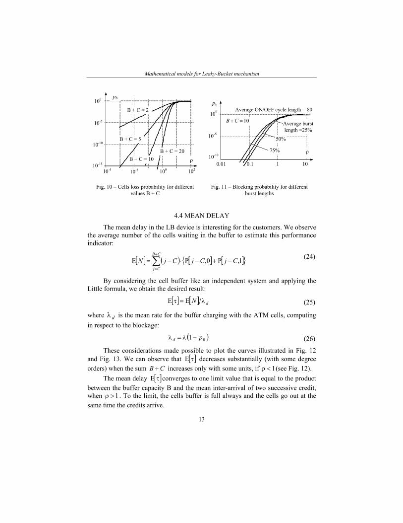
The Fig. 10 and Fig. 11 present some curves of the blocking probabilities versus the indicator ρ . In the first case we observe that for 1<ρ (usual case in practice) if the sum CB + increases with some units, then the blocking probability decreases with some measure degrees. The curves plotted in Fig. 11 show the relative constant sensitivity of the blockage with the burst variation. In other words, the punishment is proportional with the "filling factor" of the ON/OFF cycle for a large scale of the usage indicator ρ .

Also from the Fig. 11 we observe that the blockage decreases if the filling factor decreases, when the ρ rest constant. The explanation is: if the filling factors decrease, then the global rate λ over a cycle ON/OFF decreases, see relation (20), and consequently ρ decreases too. So, if ρ must rest constantly when the filling factor decrease, then the arrival rates in the two states must increase; this fact produces the blockage increasing.


13

B + C = 2

B + C = 5

B + C = 10 B + C = 20

10210010-2 10-4 10-15

10-10

10-5

100 pb

ρ

Average ON/OFF cycle length = 80

10=+ CB

10 1 0.10.01

100

10-5

10-10

pb

Average burst length =25%

50%

75% ρ

Fig. 10 – Cells loss probability for different values B + C

Fig. 11 – Blocking probability for different burst lengths

4.4 MEAN DELAY

The mean delay in the LB device is interesting for the customers. We observe the average number of the cells waiting in the buffer to estimate this performance indicator:

[ ] ( ) [ ] [ ]{ }∑+

=

−+−⋅−=CB

Cj

CjCjCjN 1,P0,PE (24)

By considering the cell buffer like an independent system and applying the Little formula, we obtain the desired result:

[ ] [ ] dN λ=τ EE (25)

where dλ is the mean rate for the buffer charging with the ATM cells, computing in respect to the blockage:

( )Bd p−λ=λ 1 (26)

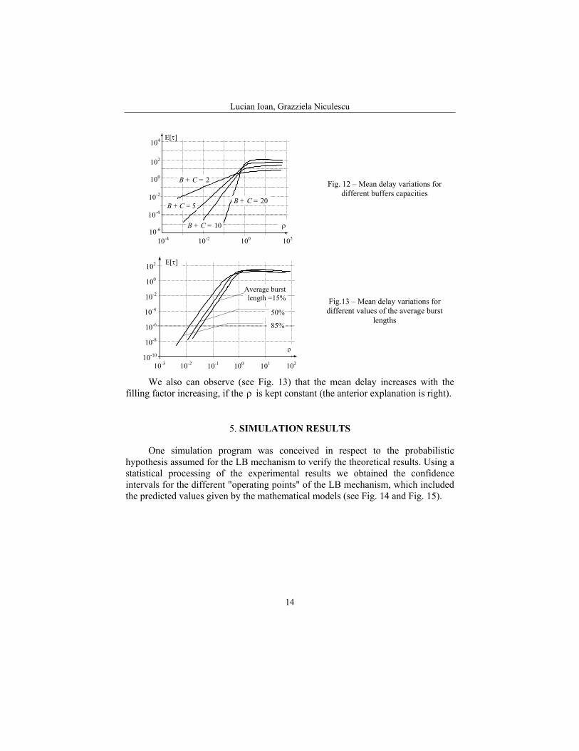
These considerations made possible to plot the curves illustrated in Fig. 12 and Fig. 13. We can observe that [ ]τE decreases substantially (with some degree orders) when the sum CB + increases only with some units, if 1<ρ (see Fig. 12).

The mean delay [ ]τE converges to one limit value that is equal to the product between the buffer capacity B and the mean inter-arrival of two successive credit, when 1>ρ . To the limit, the cells buffer is full always and the cells go out at the same time the credits arrive.


14

ρ

E[τ]

10-4 10-2 100 10210-6

10-4

10-2

100

102

104

B + C = 2

B + C = 5

B + C = 10

B + C = 20

Fig. 12 – Mean delay variations for different buffers capacities

Average burst length =15%

50%

85%

10-3 10-2 10-1 100 101 10210-10

10-8

10-6

10-4

10-2

100

102

ρ

E[τ]

Fig.13 – Mean delay variations for different values of the average burst

lengths

We also can observe (see Fig. 13) that the mean delay increases with the filling factor increasing, if the ρ is kept constant (the anterior explanation is right).

5. SIMULATION RESULTS

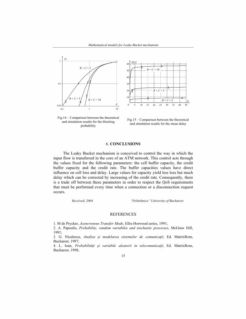
One simulation program was conceived in respect to the probabilistic hypothesis assumed for the LB mechanism to verify the theoretical results. Using a statistical processing of the experimental results we obtained the confidence intervals for the different "operating points" of the LB mechanism, which included the predicted values given by the mathematical models (see Fig. 14 and Fig. 15).


15

10 1 0.1 0.01

0.1

1

B + C = 2

B + C = 5 B + C = 10ρ

pb

E[τ]

5 10

B + C = 10

B + C = 5

B + C = 2 ρ

15 20 25 30 35 40 45 0

10

20

30

40

50

60

Fig.14 – Comparison between the theoretical and simulation results for the blocking

probability Fig.15 – Comparison between the theoretical

and simulation results for the mean delay

6. CONCLUSIONS

The Leaky Bucket mechanism is conceived to control the way in which the input flow is transferred in the core of an ATM network. This control acts through the values fixed for the following parameters: the cell buffer capacity, the credit buffer capacity and the credit rate. The buffer capacities values have direct influence on cell loss and delay. Large values for capacity yield less loss but much delay which can be corrected by increasing of the credit rate. Consequently, there is a trade off between these parameters in order to respect the QoS requirements that must be performed every time when a connection or a disconnection request occurs.

Received, 2004 “Politehnica“ University of Bucharest

REFERENCES

1. M de Prycker, Asyncronous Transfer Mode, Ellis-Horwood series, 1991; 2. A. Papoulis, Probability, random variabiles and stochastic processes, McGraw Hill, 1991; 3. G. Niculescu, Analiza şi modelarea sistemelor de comunicaţii, Ed. MatrixRom, Bucharest, 1997; 4. L. Ioan, Probabilităţi şi variabile aleatorii in telecomunicaţii, Ed. MatrixRom, Bucharest, 1998;


16

5. G. Niculescu, Traficul în reţelele de telecomunicaţii, Ed. Tehnică, Bucharest, 1995; 6. P. Oechslin, On-off sources and worst case arrival patterns of the Leaky Bucket, technical report, University College London, September 1997; 7. H. Roset, A. Gravey, A.L. Beylot, M. Becker, The CDV along a Path of a Network: Analysis of the Leaky Bucket Mechanism, 8th Workshop on performance Modeling and ATM Networks, Bradford, UK, July, 2000; 8. J. Carrasco, S. Mahevas, G. Rubino, V. Sune, A Model of the Leaky Bucket ATM Generic Flow control Mechanism: A Case Study on Solving Large Cyclic Models, IEE Proc. Comms., 148(3), pages 188-196, June 2001; 9. H.M. Guizani, An Effective congestion Control Scheme for ATM Networks, International Journal of Network Management, vol. 8, Issue 2, March-April 1998, pages 75-86; 10. M.A. Rahman, Guide to ATM Systems and Technology, Artech House, Boston-London, 1998; 11. V.F. Nicola, G.A. Hagesteijn, B.G Kim, Fast Simulation of the Leaky Bucket Algorithm, Proceedings of the 26th Conference on Winter Simulation, December 1994.

Documents

TWO MATHEMATICAL MODELS FOR PERFORMANCE …lucian/en/revueroumain05.pdf · TWO MATHEMATICAL MODELS FOR PERFORMANCE EVALUATION OF LEAKY-BUCKET ALGORITHM LUCIAN IOAN, GRAZZIELA NICULESCU