Two improved algorithms for envelope and wavefront reduction

BIT 37:3 (1997), 559-590.

TWO IMPROVED ALGORITHMS FOR ENVELOPE AND WAVEFRONT REDUCTION *

GARY KUMFERT 1 and ALEX POTHEN 1'2 t

1 Department of Computer Science, Old Dominion University, Norfolk VA P3529-0162 U.S.A. email: [email protected], [email protected]

2 ICASE, NASA Langley Research Center, Hampton VA 23681-0001 U.S.A. email: [email protected]

A b s t r a c t .

Two algorithms for reordering sparse, symmetric matrices or undirected graphs to reduce envelope and wavefront are considered. The first is a combinatorial algorithm introduced by Sloan and further developed by Duff, Reid, and Scott; we describe enhancements to the Sloan algorithm that improve its quality and reduce its run time. Our test problems fall into two classes with differing asymptotic behavior of their envelope parameters as a function of the weights in the Sloan algorithm. We describe an efficient O(n log n + ra) time implementation of the Sloan algorithm, where n is the number of rows (vertices), and m is the number of nonzeros (edges). On a collection of test problems, the improved Sloan algorithm required, on the average, only twice the time required by the simpler RCM algorithm while improving the mean square wavefront by a factor of three. The second algorithm is a hybrid that combines a spectral algorithm for envelope and wavefront reduction with a refinement step that uses a modified Sloan algorithm. The hybrid algorithm reduces the envelope size and mean square wavefront obtained from the Sloan algorithm at the cost of greater running times. We illustrate how these reductions translate into tangible benefits for frontal Cholesky fa~torization and incomplete factorization preconditioning.

A M S subject classification: 65F50, 68R10, 65F10.

Key words: Envelope reduction, Laplacian matrices, reordering algorithms, spectral methods, Sloan Algorithm, sparse matrices, wavefront reduction.

1 I n t r o d u c t i o n .

We consider two a lgor i thms for reducing the envelope and wavefront of sparse, symmet r i c mat r ices or und i rec ted graphs. The first a lgor i thm was in t roduced by Sloan [39], improved fur ther by Duff, Reid, and Scot t [11], and is cur ren t ly the bes t combina to r i a l a lgo r i thm for th is problem. We descr ibe enhancements to S loan ' s a lgo r i thm t h a t (i) reduce the envelope and wavefront size further ,

*Received December 1995. Revised February 1997. tThis work was partially supported by the U. S. National Science Foundation grants CCR-

9412698, DMS-9505110, and ECS-9527169, by U. S. Department of Energy grant DE-FG05- 94ER25216, and by the National Aeronautics and Space Administration under NASA Contract NAS1-19480 while the second author was in residence at the Institute for Computer Applica- tions in Science and Engineering (ICASE), NASA Langley Research Center, Hampton, VA.

5 6 0 G. KUMFERT AND A. P O T H E N

and (ii) reduce its asymptotic time complexity and practical execution times. The second algorithm is a new hybrid algorithm that combines an algebraic (spectral) algorithm for envelope reduction described by Barnard, Pothen, and Simon [4] with the Sloan algorithm as a post-processing step. The spectral algorithm takes a "global" viewpoint of the problem, but could potentially be improved by combining it with a "local" refinement algorithm. The spectral algorithm is known to produce envelope and wavefront sizes significantly smaller than previous algorithms [4]. The hybrid algorithm further reduces the envelope size and wavefronts over the spectral and Sloan algorithms. We present a few examples to show that these improved orderings could lead to faster frontal solves and more efficient incomplete factorization preconditioners.

Sloan [39] described an implementation of his algorithm for unweighted graphs. The idea of Sloan's algorithm is to number vertices from one endpoint of an approximate diameter in the graph, choosing the next vertex to number from among the neighbors of currently numbered vertices and their neighbors. A vertex of maximum priority is chosen from this eligible subset of vertices; the priority of a vertex has a "local" term that attempts to reduce the incremental increase in the wavefront, and a "global" term that reflects its distance from the second endpoint of the approximate diameter.

Duff, Reid, and Scott [11] have extended this algorithm to weighted graphs obtained from finite element meshes, and have used these orderings for frontal factorization methods. The weighted implementation is faster for finite element meshes when several vertices have common adjacency relationships. They have also described variants of the Sloan algorithm that work directly with the elements (rather than the nodes of the elements). The Sloan algorithm is a remark- able advance over previously available algorithms such as RCM [6], Gibbs-Poole- Stockmeyer [18, 29], and Gibbs-King [17] algorithms since it computes smaller envelope and wavefront sizes.

For the most part, we follow Sloan and Duff, Reid, and Scott in our work on the Sloan algorithm. Our new contributions are the following:

We show that the use of a heap instead of an array to maintain the priorities of vertices leads to a lower time complexity, and an implementation that is about four times faster on our test problems. Sloan had implemented both versions, preferring the array over the heap for the smaller problems he worked with, and had reported results only for the former. Duff, Reid, and Scott had followed Sloan in this choice.

Our implementation of the Sloan algorithm for vertex-weighted graphs mimics what the algorithm would do on the corresponding unweighted graph, unlike the Duff, Reid, and Scott implementation. Hence we define the key parameters in the algorithm differently, and this results in smaller wavefront sizes.

We examine the weights of the two terms in the priority function to show that our test problems fall into two classes with different asymptotic behav- iors of their envelope parameters; by choosing different weights for these

A L G O R I T H M S F OR E N V E L O P E AND W A V E F R O N T R E D U C T I O N 561

two classes, we reduce the wavefront sizes obtained from the Sloan algorithm, on the average, to 60% of the original Sloan algorithm on a set of eighteen test problems.

Together, these enhancements enable the Sloan algorithm to compute small envelope and wavefront sizes fast--the time it needs is in general between two to five times that of the simpler RCM algorithm.

This paper is the third in a series on spectral algorithms for envelope and wavefront reduction. We will now summarize the findings in the first two papers to put our work on the hybrid algorithm in context.

Barnard, Pothen, and Simon [4] described a spectral algorithm that associates a Laplacian matrix with the given symmetric matrix, computes an eigenvector corresponding to the smallest positive Laplacian eigenvalue, and then computes the permutation by sorting the components of the eigenvector in monotonically increasing or decreasing order.

Unlike the rest of the algorithms that are combinatorial in nature, the spectral algorithm is algebraic, and hence its good envelope-reduction properties are intriguing. George and Pothen [16] analyzed the algorithm theoretically, by considering a related problem called the 2-sum problem. They showed that minimizing the 2-sum over all permutations is equivalent to a quadratic assignment problem, in which the trace of a product of matrices is minimized over the set of permutation matrices. This problem is NP-comptete; however, lower bounds for the 2-sum could be obtained by minimizing over the set of orthogonal and doubly stochastic matrices. (Permutation matrices satisfy the additional property that their elements are nonnegative; this property is relaxed to obtain a lower bound.) This technique gave tight lower bounds for the 2-sum for many finite-element problems, showing that the 2-sums from the spectral ordering were nearly optimal (within a few percent typically). They also showed that the permutation matrix closest to the orthogonal matrix attaining the lower bound is obtained (to first order) by permuting the second Laplacian eigenvector in monotonic order. This justifies the spectral algorithm for minimizing the 2-sum. These authors also showed that a family of graphs with small (n n) separators has small mean square wavefront (at most O(nl+'~)), where n is the number of vertices in the graph, and the exponent ~/_> 1/2 determines the separator size.

The analysis of the spectral algorithm suggests that while spectral orderings may also reduce related quantities such as the envelope size and the work in an envelope factorization, they might be improved further by post-processing with a combinatorial reordering algorithm. We explore this issue further by using the second step of the Sloan algorithm in the post-processing step; the resulting algorithm is called the hybrid algorithm in the rest of this paper.

We list some work on related problems. Juvan and Mohar [27, 28] have considered spectral methods for minimizing the/)-sum problem (for p _> 1), and Paulino et al. [35, 36] have applied spectral orderings to minimize envelope sizes. Addi- tionally, spectral methods have been applied successfully in areas such as graph partitioning [26, 37, 38], the seriation problem [3], and DNA sequencing [20].

562 G. K U M F E R T A N D A. P O T H E N

The rest of this paper is organized as follows. In Section 2, we review background information. First we define various envelope parameters, delve into the details of the spectral algorithm, and then describe a problem where the spectral algorithm performs poorly but where the hybrid algorithm does well. Section 3 describes the details of a weighted Sloan algorithm; we show how the envelope parameters vary as a function of the weights in the priority function. We analyze the time complexity of our efficient implementation (in the Appendix), and show that it runs about four times faster, on the average, than previous implementations. In Section 4, we then describe the hybrid algorithm, which refines the spectral ordering by means of the second step of a modified Sloan algorithm. In Section 5, we present results from the RCM, Sloan, spectral, and hybrid ordering algorithms for a collection of problems. Comparisons are made across four envelope parameters (envelope size, bandwidth, maximum wavefront, and mean-square wavefront), and running time. Section 6 presents some preliminary results from using the hybrid ordering in frontal Cholesky and incomplete factorization preconditioning. Conclusions and directions for future work are included in Section 7.

2 Background.

We provide definitions of various envelope parameters in Section 2.1, and review the spectral algorithm for envelope and wavefront reduction in Section 2.2. Then in Section 2.3, we motivate the hybrid algorithm by describing a class of problems where a poor spectral ordering is improved by the Sloan post- processing step in the hybrid.

2.1 Definitions and notation.

Consider a sparse symmetric n • n matrix A = [aij], whose diagonal elements are all nonzero. We consider only the lower triangle of A (including the diagonal). Let fi (A) denote the column index of the first nonzero element of the i th row. The row width of the ith row, rwi(A), is the difference between i and f i (A) , or equivalently,

rwi(A) = max { i - j } . jDa~j~O

The envelope of a matrix is defined as

E n v ( A ) = { ( i , j ) : f i ( A ) < j < i , l < i < n} .

The envelope of a symmetric matrix is easily visualized: picture the lower triangle of the matrix, and remove the diagonal and the leading zero elements in each row. The remaining elements (whether nonzero or zero) are in the envelope of the matrix. The number of these elements is the envelope size, Esize(A) = IEnv(A)l, which can also be expressed as

n

Esize(A)-- ~-~ rwi(A). i = 1

A L G O R I T H M S F O R E N V E L O P E AND W A V E F R O N T R E D U C T I O N 563

Sloan [39] uses the term profile which denotes the envelope size plus the number of elements on the diagonal.

Another envelope parameter is the bandwidth of a matrix, defined as

bw(A) = max {rwi(A)}. l < i < n

Consider the ith step of Cholesky factorization where only the lower triangle of A is stored. An equation (row) k is active at the ith step if k _> i and there exists a column l < i such that akz ~ O. The ith wavefront of A, wfi(A), is the set of active equations during the ith step of Cholesky factorization. We can describe the ith wavefront in three ways that are more intuitive. It is the set of rows that have nonzeros in the submatrix consisting of the first i columns of A and rows i to n. It is also the set of rows in the ith column that are within the envelope of the matrix, where the ith row is also included. We can also define the ith wavefront in terms of the adjacency graph of A. If X is a set of vertices in a graph, then its adjacency set

In the adjacency graph of A, the ith wavefront consists of the vertex i together with the set of vertices adjacent to the vertices numbered from 1 to i. Formally, the ith wavefront is

(2.1) wf4(A) = v4 t2 adj({vl, v2 , . . . , vi}).

The n wavefront sizes (one for each column) can be characterized by the values maximum wave front and mean-square wave front

(2.2) maxwf(A) = max {Iwf~(A)l} l < i < n

n

mswf(A) = 1 E [ w f 4 ( A ) [ 2 . n

i=1

The maximum wavefront size measures the maximum storage needed for a frontal matrix during a frontal factorization, while the mean square wavefront measures the number of floating point operations in the factorization. Duff, Erisman, and Reid [9] discuss the application of wavefront reducing orderings to frontal factorization. It is easy to verify the identity

(2.3) ~- '~ . ]wf , (A)]=n+ ~7"~rw4(A) = n - ~ - E s i z e .

4=1 4=1

The envelope and wavefront parameters depend on the order in which vertices of the graph are numbered and are independent of the numerical values of the actual matrix elements. This process of vertex numbering permutes the corresponding matrix symmetrically by rows and columns. Formally, we construct a

564 G. KUMFERT AND A. POTHEN

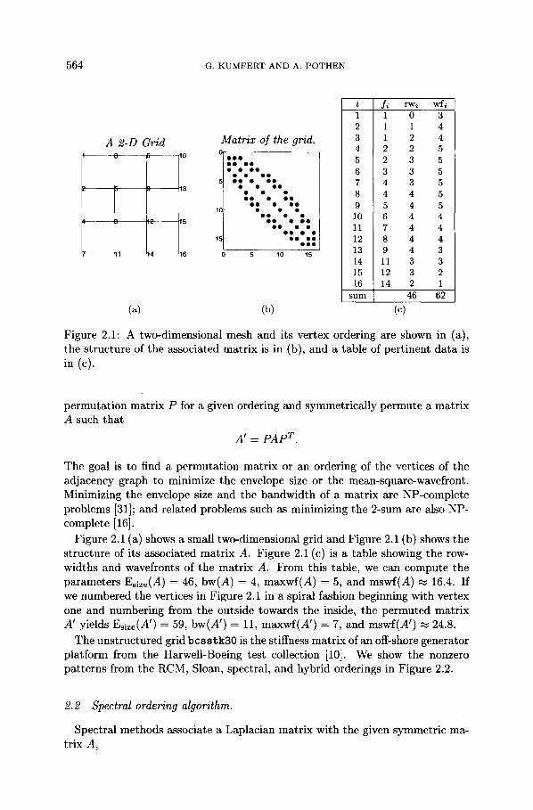
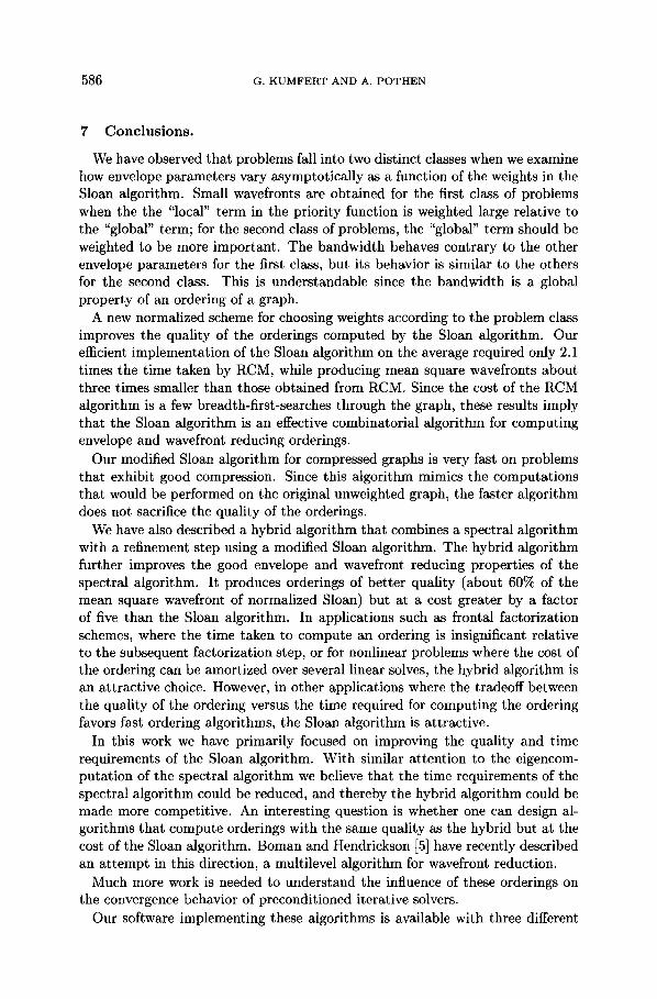
A 2-D Grid

12 15

Matrix of the grid. @@@ @@ @@

@@@@@@@@

@@ �9 @@ �9 �9 @@

@ 0 �9 Q I ~ g 1 0

0 0 �9 @@ �9 ~ 0

@@ �9 �9 O I �9 �9

Q@ 1 0 @@Q

5 10 15

(a) (b)

i fi rwi wfi 1 1 0 3 2 1 1 4 3 1 2 4 4 2 2 5 5 2 3 5 6 3 3 5 7 4 3 5 8 4 4 5 9 5 4 5 10 6 4 4 11 7 4 4 12 8 4 4 13 9 4 3 14 11 3 3 15 12 3 2 16 14 2 1

sum 46 62

(c)

Figure 2.1: A two-dimensional mesh and its vertex ordering are shown in (a), the structure of the associated matrix is in (b), and a table of pertinent data is in (c).

permutation matrix P for a given ordering and symmetrically permute a matrix A such that

A' = PAP T.

The goal is to find a permutation matrix or an ordering of the vertices of the adjacency graph to minimize the envelope size or the mean-square-wavefront. Minimizing the envelope size and the bandwidth of a matrix are NP-complete problems [31]; and related problems such as minimizing the 2-sum are also NP- complete [16].

Figure 2.1 (a) shows a small two-dimensional grid and Figure 2.1 (b) shows the structure of its associated matrix A. Figure 2.1 (c) is a table showing the row- widths and wavefronts of the matrix A. From this table, we can compute the parameters Esize(A) -- 46, bw(A) = 4, maxwf(A) -- 5, and mswf(A) ~ 16.4. If we numbered the vertices in Figure 2.1 in a spiral fashion beginning with vertex one and numbering from the outside towards the inside, the permuted matrix A' yields Esize(A') -- 59, bw(A') = 11, maxwf(A') = 7, and mswf(A') ~ 24.8.

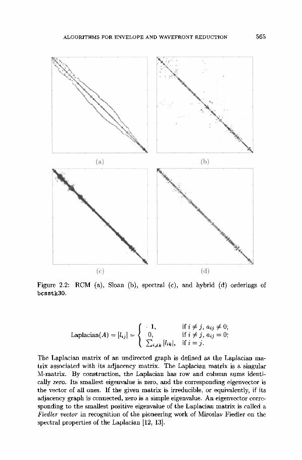
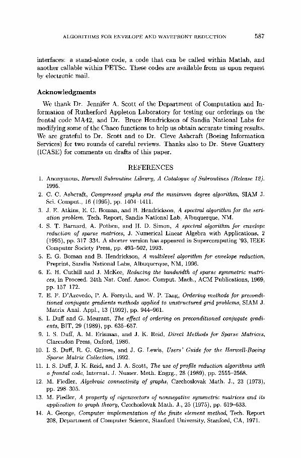
The unstructured grid bcss tk30 is the stiffness matrix of an off-shore generator platform from the Harwell-Boeing test collection [10]. We show the nonzero patterns from the RCM, Sloan, spectral, and hybrid orderings in Figure 2.2.

2.2 Spectral ordering algorithm.

Spectral methods associate a Laplacian matrix with the given symmetric matrix A,

A L G O R I T H M S F O R E N V E L O P E A N D W A V E F R O N T R E D U C T I O N 565

Figure 2.2: RCM (a), Sloan (b), spectral (c), and hybrid (d) orderings of bcsstk30.

Laplacian(A) = [lij] = -1 , if i ~ j , aij ~ 0; 0, if i ~ j , aij - ~ 0;

~-~i~k Ilikl, if i = j .

The Laplacian matrix of an undirected graph is defined as the Laplacian matrix associated with its adjacency matrix. The Laplacian matrix is a singular M-matrix. By construction, the Laplacian has row and column sums identi- cally zero. Its smallest eigenvalue is zero, and the corresponding eigenvector is the vector of all ones. If the given matrix is irreducible, or equivalently, if its adjacency graph is connected, zero is a simple eigenvalue. An eigenvector corresponding to the smallest positive eigenvalue of the Laplacian matrix is called a Fiedler vector in recognition of the pioneering work of Miroslav Fiedler on the spectral properties of the Laplacian [12, 13].

566 G. K U M F E R T AND A. P O T H E N

The spectral ordering is obtained by sorting the components of the Fiedler vector in monotonically nonincreasing or nondecreasing order. The same permutation is applied to the original matrix to obtain the spectral ordering. George and Pothen [16] show that reversing the ordering will change (improve or deteri- orate) the envelope size by a multiplicative factor that is at most the maximum degree of a vertex in the graph.

We do not need to compute the Fiedler vector very accurately for these applications. Since a multilevel algorithm is used to compute the Fiedler vector for the large problems that we consider, the practical implementations of our algorithms sometimes work with misconverged Fiedler vectors. Our experience is that these misconverged vectors work quite well in this application. Greater reductions in the envelope parameters result from investing in a local refinement algorithm, such as the Sloan algorithm, than by computing the Fiedler vector more accurately. Similar observations have been made when multilevel algorithms are used in graph partitioning [24].

We find that on many finite element problems spectral orderings do well in a global sense, but often do poorly on a local scale. It is exactly this amenability to local refinement that we seek to exploit with our hybrid algorithm.

2.3 Counter-examples for spectral envelope reduction.

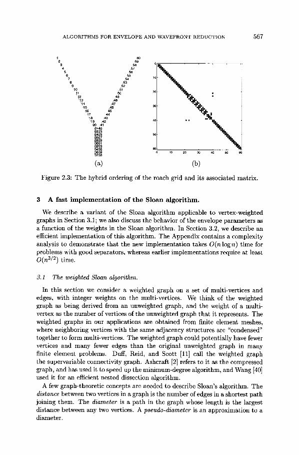
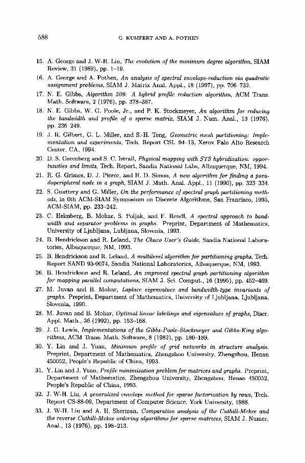
The spectral algorithm computes the lowest wavefront and envelope sizes over current algorithms for many finite element meshes as the results in Section 5 will show. However, there are problems on which the spectral method can perform poorly, as can be seen in the results presented in Subsection 5.2. Here we consider an example due to Guat tery and Miller [22] where a spectral partitioning algorithm fails to find a good cut if the part sizes must be balanced. This turns out to be one on which the spectral ordering algorithm does badly as well. We show that the hybrid algorithm, in which the spectral ordering is refined by the Sloan algorithm in a post-processing step, does well on this problem.

Figure 2.3 shows an example of the "roach" graph and the ordering computed by the hybrid algorithm. The roach graph is a ladder with the top 2/3 of the rungs removed. For a given positive integer k, this graph has 6k vertices: 2k along each "antenna", and 2k vertices on the ladder. The spectral ordering of this graph would begin numbering from the endpoint of one of the antennae, march along the outline of the graph, and end at the endpoint of the other antenna. This leads to an envelope size of 2k 2, and a mean square wave front of k2/18. (Only leading terms are shown.) It can be seen in Figure 2.3 that the hybrid algorithm numbers nodes along one antenna, then alternates across the rungs of the ladder, and finally numbers the second antenna. This leads to an envelope size of 10k, and a mean square wavefront of (2/3)k, an order of magnitude decrease in both.

For the benefit of the reader familiar with graphs constructed from the cross- product of a path and double tree, described in [22], we mention that the pro- posed hybrid algorithm exhibits similar behavior.

ALGORITHMS FOR E N V E L O P E AND WAVEFRONT REDUCTION 5 6 7

! .60 .59

"G .58 "'~ .57

5 56 6 /55

7 .54 6 ,53

'9 ,52 '10 ,51 'I I /50

'J2 .49 '13 .48

�9 14 .47 '15 .46

'16 .45 "17 .44

'18 .43 "19 ,42

"'20 ,41 '~2t,40 P-2'23

N~ ,o 2'o ;o 4o s'o 6o

(a) (b)

Figure 2.3: The hybrid ordering of the roach grid and its associated matrix.

3 A fast i m p l e m e n t a t i o n o f t h e Sloan a l g o r i t h m .

We describe a variant of the Sloan algorithm applicable to vertex-weighted graphs in Section 3.1; we also discuss the behavior of the envelope parameters as a function of the weights in the Sloan algorithm. In Section 3.2, we describe an efficient implementation of this algorithm. The Appendix contains a complexity analysis to demonstrate that the new implementation takes O(n log n) time for problems with good separators, whereas earlier implementations require at least O(n 3/2) time.

3.1 The weighted Sloan algorithm.

In this section we consider a weighted graph on a set of multi-vertices and edges, with integer weights on the multi-vertices. We think of the weighted graph as being derived from an unweighted graph, and the weight of a multi- vertex as the number of vertices of the unweighted graph that it represents. The weighted graphs in our applications are obtained from finite element meshes, where neighboring vertices with the same adjacency structures are "condensed" together to form multi-vertices. The weighted graph could potentially have fewer vertices and many fewer edges than the original unweighted graph in many finite element problems. Duff, Reid, and Scott [11] call the weighted graph the supervariable connectivity graph. Ashcraft [2] refers to it as the compressed graph, and has used it to speed up the minimum-degree algorithm, and Wang [40] used it for an efficient nested dissection algorithm.

A few graph-theoretic concepts are needed to describe Sloan's algorithm. The distance between two vertices in a graph is the number of edges in a shortest path joining them. The diameter is a path in the graph whose length is the largest distance between any two vertices. A pseudo-diameter is an approximation to a diameter.


Sloan's algorithm [39] is a graph traversal algorithm that has two parts. The first part is a heuristic algorithm that selects a start vertex s and an end vertex e that form the endpoints of a pseudo-diameter. The second part then numbers the vertices, beginning from s, and chooses the next vertex to number from a set of eligible vertices by means of a priority function. Roughly, the priority of a vertex has a dynamic and static component: the dynamic component favors a vertex that increases the current wavefront the least, while the static part favors vertices at the greatest distance from the end vertex e. The computation- intensive part of the algorithm is maintaining the priorities of the eligible vertices correctly as vertices are numbered.

We follow Duff, Reid, and Scott in their efficient scheme to compute the pseudo-diameter in the first step of the Sloan algorithm.

El ig ib le Ver t ices . Vertices are in four mutually exclusive states at each step of the algorithm. Any vertex that has already been numbered in the algorithm is a numbered vertex. Active vertices are unnumbered vertices that are adjacent to some numbered vertex. Vertices that are adjacent to active vertices but are neither active nor numbered are called preactive vertices. All other vertices are inactive. Initially all vertices are inactive, except for s, which is preactive.

At any step k, the sum of the sizes of the active vertices is exactly the size of the wavefront at that step for the reordered matrix, wfk(pApT), where P is the current permutation. Active and preactive vertices comprise the set of vertices eligible to be numbered in future steps.

An eligible vertex with the maximum priority is chosen to be numbered next. The priority function of a vertex i has two components: incr(i), the increase in the wavefront size (the number of additional vertices that enter the wavefront) if i were to be numbered next, and dist(i, e), its distance from the end vertex e.

I n c r e a s e in W a v e f r o n t Size. Our implementation of the weighted Sloan algorithm on the weighted graph mimics what the Sloan algorithm would do on an unweighted graph, and thus we define the degrees of the vertices and incr(i) differently from Duff, Reid, and Scott [11].

We denote by size(i) the integer weight of a multi-vertex i. The degree of the multi-vertex i, deg(i), is the sum of the sizes of its neighboring multi-vertices. Let the current degree of a vertex i, cdeg(i), denote the sum of the sizes of the neighbors of i among preactive or inactive vertices. It can be computed by subtracting from the degree of i the sum of the sizes of its neighbors that are numbered or active. When an eligible vertex is assigned the next available number, its preactive or inactive neighbors move into the wavefront. Thus

cdeg(i) -t- size(i), if i is preactive; (3.1) incr(i) = [ cdeg(i), if i is active.

The size(i) term for a preactive vertex i accounts for the inclusion of i into the wavefront. (Recall that the definition of the wavefront includes the diagonal element.) Initially, incr(i) is deg(i) + size(i) since nothing is in the wavefront yet.

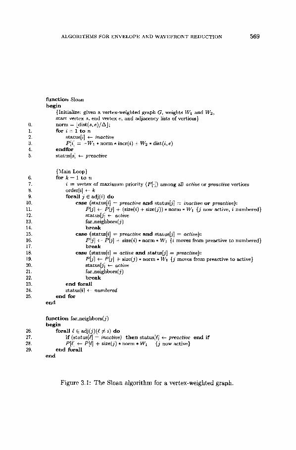
ALGORITHMS FOR ENVELOPE AND WAVEFRONT REDUCTION 569

0. 1. 2. 3. 4. 5.

6. 7. 8. 9.

10. 11. 12. 13. 14. 15. 16. 17. 18. 19. 20. 21. 22. 23. 24. 25.

26. 27. 28. 29.

f u n c t i o n Sloan b e g i n

{Initialize: given a ver tex-weighted g raph G, weights WI and W2, s t a r t ver tex s, end ver tex e, and adjacency lists of vertices} n o r m = [dist(s , e ) / A ] ; fo r i ---- 1 t o n

status[i] +- inactive P[i] = - W 1 * no rm �9 incr(i) 4- W2 * dist(i , e)

e n d fo r s ta tus[s] +- preactive

{Main Loop} fo r k ---- 1 t o n

i ---- ver tex of m a x i m u m priority (P[.]) a m o n g all active or preactive vertices order[i] +-- k f o r a l l j E adj(i) d o

c a s e (status[i] = preactive a n d s t a t u s [ j I = inactive o r preactive): P[j] +- P[j] § (size(i) + size(j)) * no rm * W1 {j now active, i numbered} s ta tus[ j ] ~- active far_neighbors( j ) b r e a k

c a s e (status[i] = preactive a n d s ta tus[ j ] = active): P[j] +-- P[j] § size(i) * no rm * W1 {i moves from preact ive to numbered} b r e a k

c a s e (status[i] = active a n d s ta tus[ j ] = preactive): P[j] +-- P[j] 4- size(j) * no rm * W~ {j moves from preact ive to active} s ta tus[ j ] ~-- active far _neighbors ( j) b r e a k

e n d fo r a l l s tatus[i] +- numbered

e n d fo r e n d

f u n c t i o n far_neighbors( j) begin

f o r a l l g E adj ( j ) (g ~ i) d o i f (status[g] = inactive) t h e n s ta tus[ t ] +- preaetive e n d i f PIg] +- Pig] + size(j) * no rm * W1 {j now active}

e n d fo r a l l e n d

F i g u r e 3 .1 : T h e S l o a n a l g o r i t h m fo r a v e r t e x - w e i g h t e d g r a p h .

5 7 0 G. K U M F E R T AND A. P O T H E N

The second component of the priority function, dist(i, e), measures the distance of a vertex i from the end vertex e. This component encourages the numbering of vertices that are very far from e even at the expense of a larger wavefront at the current step. This component is easily computed for all i by a breadth first search rooted at e.

T h e P r i o r i t y Func t i on . Denote by P(i) the priority of an eligible vertex i during a step of the algorithm. The priority function used by Sloan, and Duff, Reid and Scott is a linear combination of two components

P(i) - - - W 1 , incr(i) + W2 * dist(i, e),

where W1 and W2 are positive integer weights. At each step, the algorithm numbers next an eligible vertex i that maximizes this priority function.

The value of incr(i) ranges from 0 to (A § 1) (where A is the maximum degree of the unweighted graph G), while dist(i, e) ranges from 0 to the diameter of the graph G. We felt it desirable for the two terms in the priority function to have the same range so that we could work with normalized weights W1 and W2. Hence we use the priority function

(3.2) P(i) -- -W1 * [(dist(s, e)/A)J �9 incr(i) + W2 * dist(i, e).

If the pseudo-diameter is less than the maximum degree, we set their ratio to one. We discuss the choice of the weights later in this section.

T h e A l g o r i t h m . We present in Figure 3.1 our version of the weighted Sloan algorithm. This modified Sloan algorithm requires fewer accesses into the data structures representing the graph (or matrix) than the original Sloan algorithm. The priority updating in the algorithm ensures that incr(j) is correctly main- tained as vertices become active or preactive. When a vertex i is numbered, its neighbors and possibly their neighbors need to be examined. Vertex i must be active or preactive, since it is eligible to be numbered. We illustrate the updating of the priorities for only the first case in the algorithm, since the others can be obtained similarly. Consider the case when i is preactive and j is inactive or preactive. The multi-vertex i moves from being preactive to numbered, and hence moves out of the wavefront, decreasing incr(j) by size(i), and thereby increases P(j) by W1 * [(dist(s, e)/A)J �9 size(i). Further, since j becomes active and is now included in the wavefront, it does not contribute in the future to incr(j), and hence P(j) increases by W1 * [(dist(s, e)/A)J * size(j).

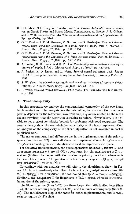
T h e Cho ice of Weigh t s . Sloan [39] and Duff, Reid, and Scott [11] recom- mend the unnormalized weights W1 -- 2, W2 = 1. We studied the influence of the normalized weights W1 and W2 on the envelope parameters, and found, to our initial surprise, that the problems we tested fell into two classes.

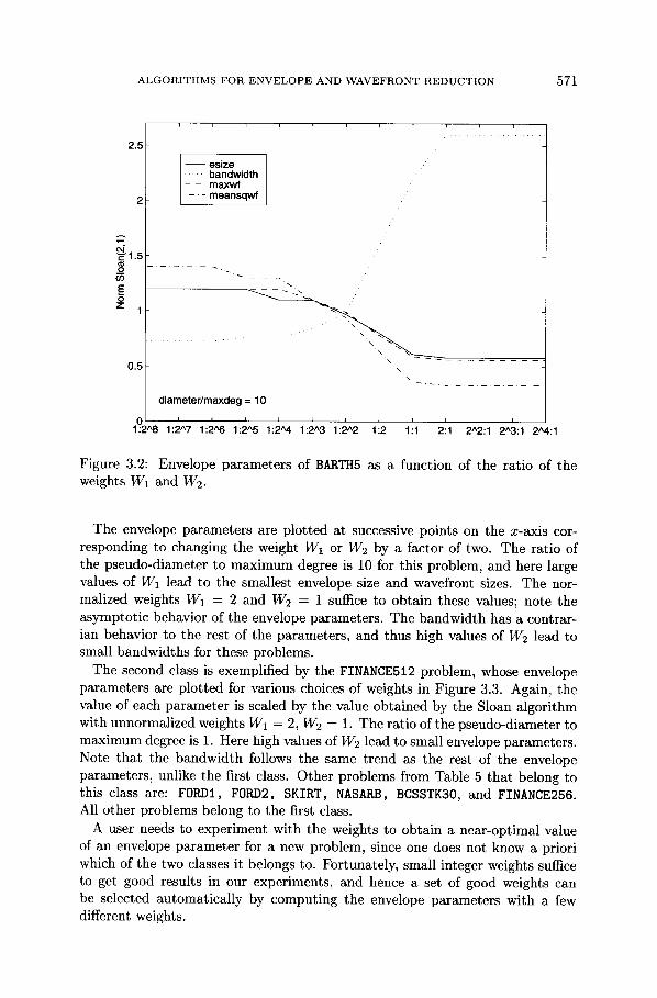
The first class is exemplified by the BARTtt5 problem, whose envelope parameters are plotted for various choices of weights in Figure 3.2. The value of each envelope parameter is scaled with respect to the value obtained with the unnormalized weights W1 -- 1 and W2 = 2 in the Sloan algorithm. Thus this and ~the next figures reveal the improvements obtained by normalizing the weights in the Sloan algorithm.


2.5

esize �9 bandwidth

- - r naxwf - - r neansqw f

~ 1 . 5 O~

z 1 ~ . . #

\ . . . . . . . . . .

0 .5 \ \

d i a m e t e r / m a x d e g = 10

0 . . . . . . ': i ': ' 1:2A8 1 :2^7 1:2."'6 1 :2 "5 1:2'*,4 1:2" '3 1 :2 "2 1 2 1 1 2 1 2 "2 :1 2A3:1 2A4:1

Figure 3.2: Envelope parameters of BARTH5 as a function of the ratio of the weights W1 and W2.

The envelope parameters are plotted at successive points on the x-axis corresponding to changing the weight W1 or W2 by a factor of two. The ratio of the pseudo-diameter to maximum degree is 10 for this problem, and here large values of W1 lead to the smallest envelope size and wavefront sizes. The normalized weights W1 = 2 and W2 = 1 suffice to obtain these values; note the asymptotic behavior of the envelope parameters. The bandwidth has a contrar- ian behavior to the rest of the parameters, and thus high values of W2 lead to small bandwidths for these problems.

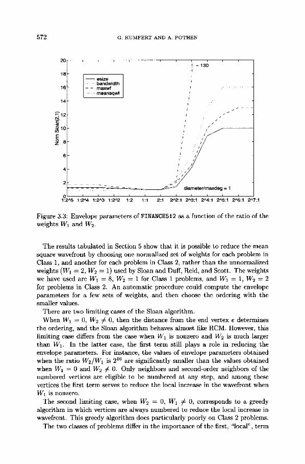
The second class is exemplified by the FINANCE512 problem, whose envelope parameters are plotted for various choices of weights in Figure 3.3. Again, the value of each parameter is scaled by the value obtained by the Sloan algorithm with unnormalized weights W1 = 2, W2 -- 1. The ratio of the pseudo-diameter to maximum degree is 1. Here high values of 1412 lead to small envelope parameters. Note that the bandwidth follows the same trend as the rest of the envelope parameters, unlike the first class. Other problems from Table 5 that belong to this class are: FORD1, FORD2, SKIRT, NASARB, BCSSTK30, and FINANCE256. All other problems belong to the first class.

A user needs to experiment with the weights to obtain a near-optimal value of an envelope parameter for a new problem, since one does not know a priori which of the two classes it belongs to. Fortunately, small integer weights suffice to get good results in our experiments, and hence a set of good weights can be selected automatically by computing the envelope parameters with a few different weights.


20 , , ,

18 esize

~__ bandwidth 16 maxwf

- meansqwf

14

~'.12

10

6

4

2

0 i I 1 1:2^5 1:2A4 1:2^3 1:2^2 1':2 1:1

- 130

f ~ I I / /

I / /

I / I /

I /

.I / /

I /

i /

I . /

=1

i { i i i L 2 1 2^2:1 2A3:1 2A4:1 2A5:1 2A6:1 2^7:1

Figure 3.3: Envelope parameters of FINANCES12 as a function of the ratio of the weights W1 and W2.

The results tabulated in Section 5 show that it is possible to reduce the mean square wavefront by choosing one normalized set of weights for each problem in Class 1, and another for each problem in Class 2, rather than the unnormalized weights (W1 = 2, W2 -- 1) used by Sloan and Duff, Reid, and Scott. The weights we have used are W1 = 8, W2 -- 1 for Class 1 problems, and W1 -- 1, W2 = 2 for problems in Class 2. An automatic procedure could compute the envelope parameters for a few sets of weights, and then choose the ordering with the smaller values.

There are two limiting cases of the Sloan algorithm. When W1 = 0, W2 r 0, then the distance from the end vertex e determines

the ordering, and the Sloan algorithm behaves almost like RCM. However, this limiting case differs from the case when W1 is nonzero and W2 is much larger than W1. In the latter case, the first term still plays a role in reducing the envelope parameters. For instance, the values of envelope parameters obtained when the ratio W2/W1 is 216 are significantly smaller than the values obtained when W1 = 0 and W2 r 0. Only neighbors and second-order neighbors of the numbered vertices are eligible to be numbered at any step, and among these vertices the first term serves to reduce the local increase in the wavefront when W1 is nonzero.

The second limiting case, when W2 -- 0, W1 ~ 0, corresponds to a greedy algorithm in which vertices are always numbered to reduce the local increase in wavefront. This greedy algorithm does particularly poorly on Class 2 problems.

The two classes of problems differ in the importance of the first, "local", term


that controls the incremental increase in the wavefront relative to the second, "global", term that emphasizes the numbering of vertices far from the end-vertex. When the first term is more important in determining the envelope parameters, the problem belongs to Class 1, and when the second term is more important, it belongs to Class 2. We have observed that the first class of problems represent simpler meshes: e.g., discretization of the space surrounding a body, such as an airfoil in the case of BARTH5. The problems in the second class arise from finite element meshes of complex three-dimensional geometrical objects, such as auto- mobile frames. The FINANCE512 problem is a linear program consisting of several subgraphs joined together by a binary tree interconnection. In these problems, it is important to explore several "directions" in the graph simultaneously to obtain small envelope parameters.

The bandwidth is smaller when larger weights are given to the second term, for both classes of problems. This is to be expected, since to reduce the bandwidth, we need to decrease, over all edges, the maximum deviation between the numbers of the endpoints of an edge.

3.2 The accelerated implementation.

In the Sloan algorithm, the vertices eligible for numbering are kept in a priority queue. Sloan [39] implemented the priority queue both as an unordered list in an array and as a binary heap, and found that the array implementation was faster for his test problems (all with less than 3,000 vertices). Hence he reported results from the array implementation only. Duff, Reid, and Scott [11] have followed Sloan in using the array implementation for the priority queue in the Harwell library routine MC40 [1].

We provide a complexity analysis of the worst-case execution time of the two implementations in the Appendix, which shows that the heap implementation runs in O(n log n) time, while the array implementation requires O(n 15) time for two-dimensional problems, and O(n 5/3) time for three-dimensional problems.

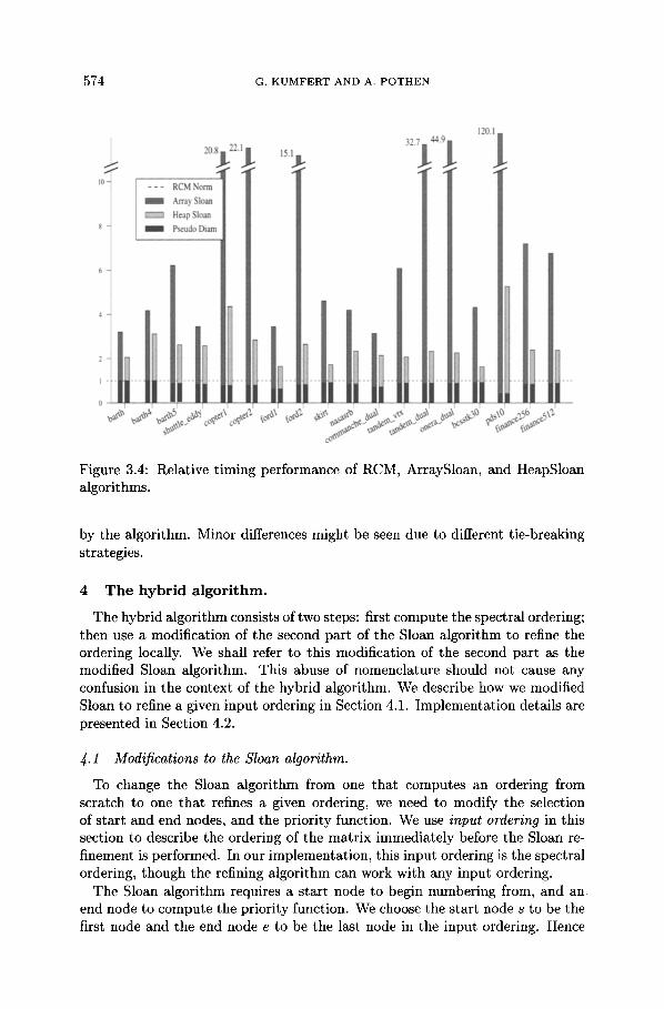
This difference in running time requirements is experimentally observed as well. In Figure 3.4 we compare the times taken by the array and heap implementations of the Sloan algorithm relative to our implementation of the RCM algorithm. The RCM algorithm uses a fast pseudo-diameter algorithm described by Duff, Reid, and Scott [11].

For the eighteen matrices in Table 5.1, the mean time of the ArraySloan was 11.3 times that of RCM, while the median time was 8.2 that of RCM. However, the mean cost of the HeapSloan was only 2.5 times that of RCM, with the median cost only 2.3. The greatest improvements are seen for the problems with greater numbers of vertices or with higher average degrees.

We have also computed the times taken by MC40B to order these problems, and found them to be comparable to the times reported here for the ArraySloan implementation, in spite of the different programming languages used (Fortran for MC40B and and C for ours.)

We emphasize that this change in the data structure for the priority queue has no significant influence on the quality of the envelope parameters computed


Figure 3.4: Relative timing performance of RCM, ArraySloan, and HeapSloan algorithms.

by the algorithm. Minor differences might be seen due to different tie-breaking strategies.

4 The hybrid algorithm.

The hybrid algorithm consists of two steps: first compute the spectral ordering; then use a modification of the second part of the Sloan algorithm to refine the ordering locally. We shall refer to this modification of the second part as the modified Sloan algorithm. This abuse of nomenclature should not cause any confusion in the context of the hybrid algorithm. We describe how we modified Sloan to refine a given input ordering in Section 4.1. Implementation details are presented in Section 4.2.

4.1 Modifications to the Sloan algorithm.

To change the Sloan algorithm from one that computes an ordering from scratch to one that refines a given ordering, we need to modify the selection of start and end nodes, and the priority function. We use input ordering in this section to describe the ordering of the matrix immediately before the Sloan refinement is performed. In our implementation, this input ordering is the spectral ordering, though the refining algorithm can work with any input ordering.

The Sloan algorithm requires a start node to begin numbering from, and an end node to compute the priority function. We choose the start node s to be the first node and the end node e to be the last node in the input ordering. Hence

ALGORITHMS FOR ENVELOPE AND WAVEFRONT REDUCTION 5"/5

the burden of finding a good set of endpoints is placed on the spectral method. Experience suggests that this is where it should be. The spectral method seems to have a broader and more consistent view than the local diameter heuristic. This feature alone yields improved envelope parameters over the Sloan algorithm for most of our test problems.

The priority function is

(4.1) P(i) = - W 1 * [(n/A)J �9 incr(i) + W2 * dist(i, e) - W3 * i.

The first two terms are similar to the priority function of the Sloan algorithm (Subsection 3.1), except that the normalization factor has n, the number of vertices in the numerator, rather than the pseudo-diameter. The latter is not computed in this context, and this choice makes the first and third terms range from 1 to n.

This function is sensitive to the initial ordering through the addition of a third weight, W3. For W3 > 0, higher priority is given to lower numbered vertices in the input ordering. Conversely, for W3 < 0, priority is given to higher numbered vertices. This effectively performs the refinement on the reverse input ordering, provided s and e are also reversed. There is some redundancy between weighting the distance from the end in terms of the number of hops (dist(i, e)) and the distance from the end in terms of the input ordering (i).

Selection of the nodes s and e and the new priority function are the only algorithmic modifications made to the Sloan algorithm. The node selection, node promotion, and priority updating scheme (see Fig. 3.1), are unchanged.

The normalization factor in the first term of the priority function makes the initial influence of the first and third terms roughly equal in magnitude when W1 and W3 are both equal to 1. The weight W2 is usually set to one. This makes it a very weak parameter in the whole algorithm, but small improvements result when its influence is nonzero. If the component of the Fiedler vector with the largest absolute value has the negative sign, we set W3 = - 1 and swap s and e. Otherwise, we set W3 = 1 and use the nondecreasing ordering of the Fiedler vector.

For Class 1 problems, higher values of W1 can lead to improvements in the envelope parameters over the choice of W1 = 1, even though it is slight in most cases. For Class 2 problems, use of W1 = 1, W2 = W3 = 2 can lead to improvements as well.

4.2 Implementation details.

All the results presented in the following section were obtained on a Sun SPARCstation 20 with 64MB physical main memory and 846MB of swap space, running SunOS 4.1.3. The software used includes Matlab 4.2a, Chaco 2.0 [24] and a suite of Matlab M-files and MEX-files 1 that we wrote. All of the MEX-files are written in C. A toolbox of M-files written by Gilbert, Miller, and Teng [19]

1Both M-files and MEX-files are programs in Matlab. M-files are interpreted and are analogous to UNIX scripts or DOS batch files. MEX files are compiled C or Fortran codes that are dynamically linked into Matlab.


Problem I VI I EI Comment BARTH BARTH4 BARTH5 SHUTTLE.EDDY COPTER1 COPTER2 FORD1 FORD2 SKIRT NASASRB COMMANCHE_DUAL TANDEM_VTX TANDEM_DUAL ONERA_DUAL BCSSTK30 PDS10 FINANCE256 FINANCE512 COMP.SKIRT COMP.NASARB COMP.BCSSTK30

6,691 19,748 6,019 17,473

15,606 45,878 10,429 46,585 17,222 96,921 55,476 352,238 18,728 41,424

100,196 222,246 45,361 1,268,228 54,870 1,311,227

7,920 11,880 18,454 117,448 84,069 183,212 85,567 116,817 28,924 1,007,284 16,558 66,550 37,376 130,560 74,752 261,120 14,944 160,461 24,953 275,796 9,289 111,442

2-D CFD problems

3-D structural problems

3-D CFD problems

3-D stiffness matrix

linear programs

compressed SKIRT compressed NASARB compressed BCSSTK30

Table 5.1: The list of eighteen test problems. For the three problems that compressed well, their compressed versions are also shown.

was used to generate some model problems, visualize results, and test code under development.

Matlab is the main platform on which the experiments were done. Its inter- active environment is very flexible to use. M-files allowed for quick prototype code generation. However, M-files are interpreted and too slow, in general, for matrices of reasonable size. The code was then re-written in C, given a Mat- lab wrapper function, and linked as a MEX file into Matlab's dynamic library. Chaco was used to obtain the Fiedler vector.

5 Comp u ta t iona l results.

We describe in Section 5.1 how we chose the computational parameters in the hybrid algorithm. In Section 5.2 we discuss the relative reductions in envelope size and wavefront of eighteen test problems obtained from RCM, Sloan, spectral, and hybrid algorithms.

ALGORITHMS FOR ENVELOPE AND WAVEFRONT REDUCTION 5 7 7

Problem mswf maxwf Esize bw

BARTH BARTH4 BARTH5 SHUTTLE COPTER1 COPTER2 FORD1 FORD2 SKIRT NASARB COMMANCHE.DUAL TANDEM.VERTEX TANDEM.DUAL ONERA.DUAL BCSSTK30 PDS10 FINANCE256 FINANCE512

Time (see.)

1.26e4 164 7.01e5 199 0.13 1.61e4 204 7.03e5 218 0.05 5.08e4 351 3.26e6 373 0.16 5.84e3 167 7.09e5 238 0.12 2.84e5 797 8.62e6 932 0.13 2.26e6 2,447 7.55e7 2,975 0.88 2.65e4 223 2.90e6 258 0.30 3.74e5 884 5.72e7 963 1.1 1.11e6 1,745 4.42e7 2,070 5.0 1.65e5 840 2.06e7 881 3.3 6.73e3 150 5.90e5 155 0.07 8.28e5 1,489 1.53e7 1,847 0.27 1.96e6 2,008 1.22e8 2,199 1.4 4.86e6 3,096 1.71e8 3,478 1.2 1.07e6 1,734 2.66e7 2,826 3.7 3.66e6 2,996 2.95e7 4,235 0.35 9.38e5 1,437 3.26e7 2,014 0.51 5.79e5 879 5.55e7 1,306 1.0

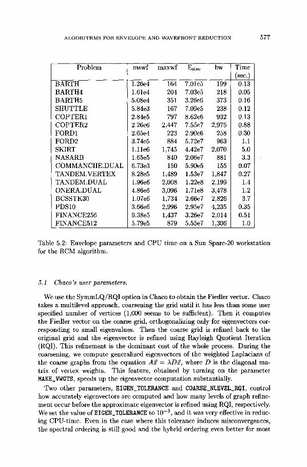
Table 5.2: Envelope parameters and CPU time on a Sun Sparc-20 workstation for the RCM algorithm.

5.1 Chaco ' s user parameters .

We use the SymmLQ/RQI option in Chaco to obtain the Fiedler vector. Chaco takes a multilevel approach, coarsening the grid until it has less than some user specified number of vertices (1,000 seems to be sufficient). Then it computes the Fiedler vector on the coarse grid, orthogonalizing only for eigenvectors corresponding to small eigenvalues. Then the coarse grid is refined back to the original grid and the eigenvector is refined using Rayleigh Quotient Iteration (RQI). This refinement is the dominant cost of the whole process. During the coarsening, we compute generalized eigenvectors of the weighted Laplacians of the coarse graphs from the equation A~ = AD~, where D is the diagonal matrix of vertex weights. This feature, obtained by turning on the parameter MAKE_VWGTS, speeds up the eigenvector computation substantially.

Two other parameters, EIGEN TOLEI~NCE and COARSE_NLEVEL_KQI, control how accurately eigenvectors are computed and how many levels of graph refinement occur before the approximate eigenvector is refined using RQI, respectively. We set the value of EIGEN_TOLF_2~NCE to 10 -3, and it was very effective in reducing CPU-time. Even in the case where this tolerance induces misconvergences, the spectral ordering is still good and the hybrid ordering even better for most


Problem SLOAN NSLOAN SPECTRAL HYBRID (Class)

BARTH BARTH4 BARTH5 SHUTTLE COPTER1 COPTER2 FORD1 FORD2 SKIRT NASARB COMMANCHE.DUAL TANDEM.VTX TANDEM.DUAL ONERA.DUAL BCSSTK30 PDS10 FINANCE256 FINANCE512 COMP.SKIRT COMP.NASARB COMP.BCSSTK30

0.48 0.43 (1) 0.43 0.30 0.40 0.21 (1) 0.20 0.15 0.56 0.18 (1) 0.18 0.14 0.60 0.60 (1) 1.0 0.65 0.71 0.45 (1) 0.74 0.53 0.39 0.27 (1) 0.28 0.16 0.67 0.67 (2) 0.48 0.39 0.51 0.51 (2) 0.44 0.33 0.57 0.50 (2) 0.44 0.37 0.74 0.75 (2) 0.99 0.71 0.60 0.34 (1) 0.37 0.23 0.16 0.12 (1) 0.14 0.10 0.53 0.28 (1) 0.14 0.11 0.44 0.21 (1) 0.09 0.07 0.37 0.30 (2) 0.10 0.05 0.20 0.13 (1) 0.75 0.15 0.04 0.04 (2) 0.07 0.04 0.05 0.06 (2) 0.14 0.05

0.46 (2) 0.51 0.39 0.68 (2) 1.8 0.75 0.26 (2) 0.13 0.06

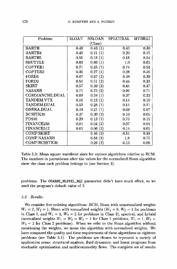
Table 5.3: Mean square wavefront sizes for various algorithms relative to RCM. The numbers in parentheses after the values for the normalized Sloan algorithm show the class each problem belongs to (see Section 3).

problems. The COARSE_NLEVEL_RQI parameter didn't have much effect, so we used the program's default value of 2.

5.2 Results.

We consider five ordering algorithms: RCM, Sloan with unnormalized weights W1 = 2, W2 = 1, Sloan with normalized weights (W1 = 8, W2 = 1 for problems in Class 1, and W1 = 1, W2 = 2 for problems in Class 2), spectral, and hybrid (normalized weights W1 -- W2 =- W3 = 1 for Class 1 problems, W1 = 1, W2 = W3 -- 2 for Class 2 problems). When we refer to the Sloan algorithm without mentioning the weights, we mean the algorithm with normalized weights. We have compared the quality and time requirements of these algorithms on eighteen problems (see Table 5.1). The problems are chosen to represent a variety of application areas: structural analysis, fluid dynamics, and linear programs from stochastic optimization and multicommodity flows. The complete set of results


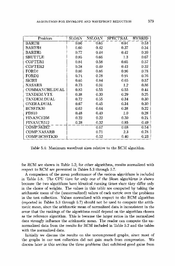
Problem SLOAN NSLOAN SPECTRAL HYBRID BARTH BARTH4 BARTH5 SHUTTLE COPTER1 COPTER2 FORD1 FORD2 SKIRT NASARB COMMANCHE.DUAL TANDEM.VTX TANDEM.DUAL ONERA.DUAL BCSSTK30 PDS10 FINANCE256 FINANCE512 COMP.SKIRT COMP.NASARB COMP.BCSSTK30

0.66 0.65 0.64 0.53 0.60 0.42 0.37 0.34 0.77 0.44 0.42 0.39 0.85 0.66 1.3 0.67 0.84 0.58 0.65 0.57 0.58 0.49 0.43 0.32 0.86 0.86 0.96 0.78 0.74 0.78 0.91 0.76 0.65 0.84 0.65 0.57 0.73 0.91 1.2 0.86 0.83 0.55 0.55 0.44 0.38 0.30 0.29 0.25 0.72 0.55 0.34 0.30 0.67 0.45 0.34 0.30 0.63 0.64 0.38 0.22 0.48 0.40 1.0 0.28 0.22 0.22 0.30 0.21 0.28 0.32 0.85 0.49

0.67 0.68 0.54 0.71 2.3 0.78 0.52 0.40 0.23

Table 5.4: Maximum wavefront sizes relative to the RCM algorithm.

for RCM are shown in Table 5.2; for other algorithms, results normalized with respect to RCM are presented in Tables 5.3 through 5.7.

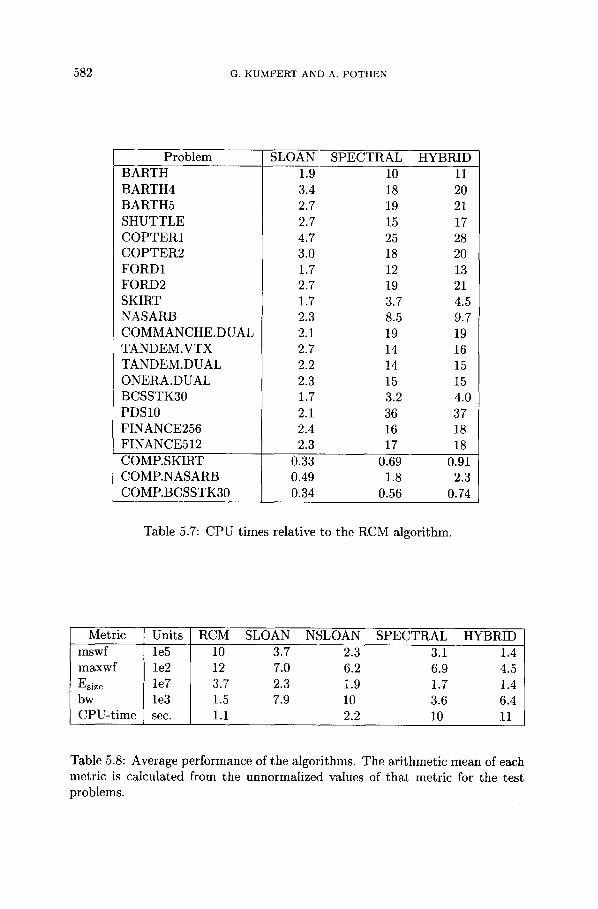
A comparison of the mean performance of the various algorithms is included in Table 5.8. The CPU time for only one of the Sloan algorithms is shown because the two algorithms have identical running times since they differ only in the choice of weights. The values in this table are computed by taking the arithmetic mean of the (unnormalized) values of each metric over the problems in the test collection. Values normalized with respect to the RCM algorithm (reported in Tables 5.3 through 5.7) should not be used to compute the arithmetic mean, since the arithmetic mean of normalized data is inconsistent in the sense that the rankings of the algorithms could depend on the algorithm chosen as the reference algorithm. This is because the larger ratios in the normalized data strongly influence the arithmetic mean. The reader can compute the unnormalized data from the results for RCM included in Table 5.2 and the tables with the normalized data.

Initially we discuss the results on the uncompressed graphs, since most of the graphs in our test collection did not gain much from compression. We discuss later in this section the three problems that exhibited good gains from


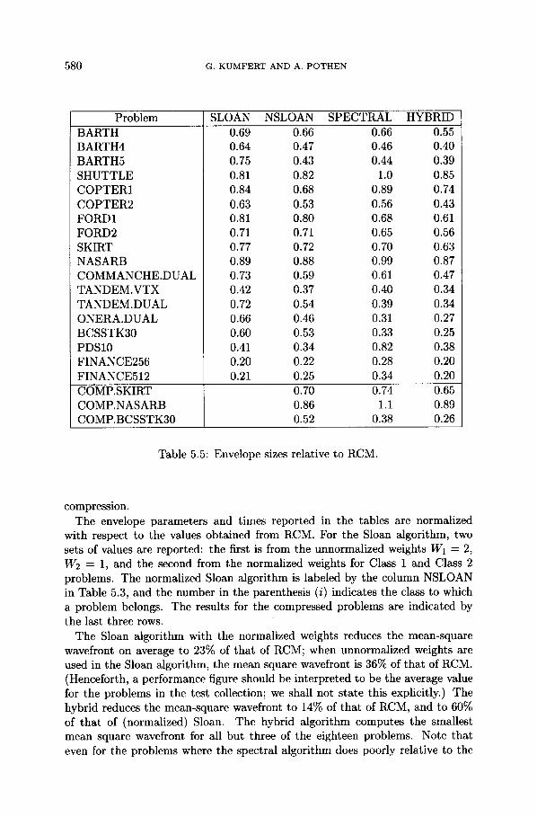
Problem SLOAN NSLOAN SPECTRAL HYBRID BARTH BARTH4 BARTH5 SHUTTLE COPTER1 COPTER2 FORD1 FORD2 SKIRT NASARB COMMANCHE.DUAL TANDEM.VTX TANDEM.DUAL ONERA.DUAL BCSSTK30 PDS10 FINANCE256 FINANCE512 COMP.SKIRT COMP.NASARB COMP.BCSSTK30

0.69 0.66 0.66 0.55 0.64 0.47 0.46 0.40 0.75 0.43 0.44 0.39 0.81 0.82 1.0 0.85 0.84 0.68 0.89 0.74 0.63 0.53 0.56 0A3 0.81 0.80 0.68 0.61 0.71 0.71 0.65 0.56 0.77 0.72 0.70 0.63 0.89 0.88 0.99 0.87 0.73 0.59 0.61 0.47 0.42 0.37 0.40 0.34 0.72 0.54 0.39 0.34 0.66 0.46 0.31 0.27 0.60 0.53 0.33 0.25 0.41 0.34 0.82 0.38 0.20 0.22 0.28 0.20 0.21 0.25 0.34 0.20

0.70 0.74 0.65 0.86 1.1 0.89 0.52 0.38 0.26

Table 5.5: Envelope sizes relative to RCM.

compression. The envelope parameters and times reported in the tables are normalized

with respect to the values obtained from RCM. For the Sloan algorithm, two sets of values are reported: the first is from the unnormalized weights W1 -- 2, W2 = 1, and the second from the normalized weights for Class 1 and Class 2 problems. The normalized Sloan algorithm is labeled by the column NSLOAN in Table 5.3, and the number in the parenthesis (i) indicates the class to which a problem belongs. The results for the compressed problems are indicated by the last three rows.

The Sloan algorithm with the normalized weights reduces the mean-square wavefront on average to 23% of that of RCM; when unnormalized weights are used in the Sloan algorithm, the mean square wavefront is 36% of that of RCM. (Henceforth, a performance figure should be interpreted to be the average value for the problems in the test collection; we shall not state this explicitly.) The hybrid reduces the mean-square wavefront to 14% of that of RCM, and to 60% of that of (normalized) Sloan. The hybrid algorithm computes the smallest mean square wavefront for all but three of the eighteen problems. Note that even for the problems where the spectral algorithm does poorly relative to the


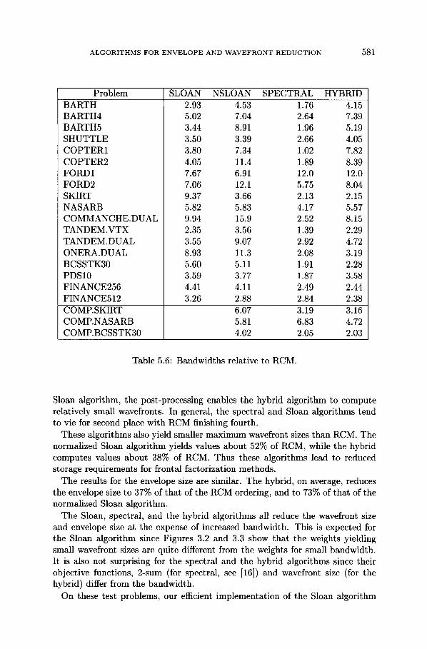
Problem SLOAN NSLOAN SPECTRAL HYBRID BARTH BARTH4 BARTH5 SHUTTLE COPTER1 COPTER2 FORD1 FORD2 SKIRT NASARB COMMANCHE.DUAL TANDEM.VTX TANDEM.DUAL ONERA.DUAL BCSSTK30 PDS10 FINANCE256 FINANCEbl2 COMP.SKIRT COMP.NASARB COMP.BCSSTK30

2.93 4.53 1.76 4.15 5.02 7.04 2.64 7.39 3.44 8.91 1.96 5.19 3.50 3.39 2.66 4.05 3.80 7.34 1.02 7.82 4.05 11.4 1.89 8.39 7.67 6.91 12.0 12.0 7.06 12.1 5.75 8.04 9.37 3.66 2.13 2.15 5.82 5.83 4.17 5.57 9.94 15.9 2.52 8.15 2.35 3.56 1.39 2.29 3.55 9.07 2.92 4.72 8.93 11.3 2.08 3.19 5.60 5.11 1.91 2.28 3.59 3.77 1.87 3.58 4.41 4.11 2.49 2.44 3.26 2.88 2.84 2.38

6.07 3.19 3.16 5.81 6.83 4.72 4.02 2.05 2.03

Table 5.6: Bandwidths relative to RCM.

Sloan algorithm, the post-processing enables the hybrid algorithm to compute relatively small wavefronts. In general, the spectral and Sloan algorithms tend to vie for second place with RCM finishing fourth.

These algorithms also yield smaller maximum wavefront sizes than RCM. The normalized Sloan algorithm yields values about 52% of RCM, while the hybrid computes values about 38% of RCM. Thus these algorithms lead to reduced storage requirements for frontal factorization methods.

The results for the envelope size are similar. The hybrid, on average, reduces the envelope size to 37% of that of the RCM ordering, and to 73% of that of the normalized Sloan algorithm.

The Sloan, spectral, and the hybrid algorithms all reduce the wavefront size and envelope size at the expense of increased bandwidth. This is expected for the Sloan algorithm since Figures 3.2 and 3.3 show that the weights yielding small wavefront sizes are quite different from the weights for small bandwidth. It is also not surprising for the spectral and the hybrid algorithms since their objective functions, 2-sum (for spectral, see [16]) and wavefront size (for the hybrid) differ from the bandwidth.

On these test problems, our efficient implementation of the Sloan algorithm

5 8 2 G. KUMFERT AND A. P O T H E N

Problem SLOAN SPECTRAL HYBRID BARTH BARTH4 BARTH5 SHUTTLE COPTER1 COPTER2 FORD1 FORD2 SKIRT NASARB

1.9 10 11 3.4 18 20 2.7 19 21 2.7 15 17 4.7 25 28 3.0 18 20 1.7 12 13 2.7 19 21 1.7 3.7 4.5 2.3 8.5 9.7 2.1 19 19 2.7 14 16 2.2 14 15 2.3 15 15 1.7 3.2 4.0 2.1 36 37 2.4 16 18 2.3 17 18

COMMANCHE,DUAL TANDEM.VTX TANDEM.DUAL ONERA.DUAL BCSSTK30 PDS10 FINANCE256 FINANCE512 COMP.SKIRT COMP.NASARB COMP.BCSSTK30

0.33 0.69 0.91 0,49 1.8 2.3 0.34 0.56 0.74

Table 5.7: CPU times relative to the RCM algorithm.

Metric Units RCM SLOAN NSLOAN SPECTRAL HYBRID mswf le5 10 3.7 2.3 3.1 1.4 maxwf le2 12 7.0 6.2 6.9 4.5 Esize le7 3.7 2.3 1.9 1.7 1.4 bw le3 1.5 7.9 10 3.6 6.4 CPU-t ime sec. 1.1 2.2 10 11

Table 5.8: Average performance of the algorithms. The arithmetic mean of each metric is calculated from the unnormalized values of that metric for the test problems,

A L G O R I T H M S F O R E N V E L O P E AND W A V E F R O N T R E D U C T I O N 583

requires on average only 2.1 times the time taken by the RCM algorithm. The hybrid algorithm requires about 5.0 times the time taken by the Sloan algorithm on the average. This ratio is always greater than one, since the hybrid algorithm uses the second step of the Sloan algorithm (numbering the vertices) to refine the spectral ordering, and the eigenvector computation is much more expensive than the first step of the Sloan algorithm (the pseudo-diameter computation). We believe that these time requirements are small for the applications that we consider: preconditioned iterative methods and frontal solvers.

Gains from Compressed Graphs. As discussed in Section 3.1, the use of the supervariable connectivity graph [11] (called the compressed graph by Ashcraft [2]) can lead to further gain in the execution times of the algorithms. Only three of the problems, SKIRT, NASARB, BCSSTK30, compressed well. This is because many of the multicomponent finite element problems in our test set had only one node representing the multiple degrees of freedom at that node. The compression feature is an important part of many software packages for solving PDE's, since it results in reduced running times and storage overheads, and our results also show impressive gains from compression.

Three problems in our test set compressed well: SKIRT, NASAKB, and BCSSTK30. Results for these problems are shown in the last three rows of each table. The numbers of multivertices and edges in the compressed graphs are also shown. For these three problems, compression speeds up the Sloan algorithm on average by a factor of nearly 5, and the hybrid algorithm by a factor of 4.6.

Compression improves the quality of the Sloan algorithm for these three problems, and does not have much impact on the hybrid algorithm. This improved quality of the compressed Sloan algorithm follows from our choice of parameters in the compressed algorithm to correspond exactly to their values in the uncompressed graph. However, on NASARB, the spectral envelope parameters de- teriorate upon compression. We do not know the reason for this, but it could be due to the poorer quality of the eigenvector computed for the weighted problem. In any case, the compressed hybrid algorithm recoups most of this deterioration.

6 Applications.

This section discusses preliminary evidence demonstrating the applicability of the orderings we generated. In Section 6.1 we describe how a reduction in mean square wavefront directly translates into a greater reduction in CPU-time in a frontal factorization. We also discuss the impact of these orderings on incomplete Cholesky (IC) preconditioned iterative solvers in Section 6.2.

6.1 Frontal methods.

The work in a frontal Cholesky factorization algorithm is

1 n work(A) = ~ ~-]lwfi(A)l ( Iwfi(A)l + 3).

i=1

584 a K U M F E R T AND A. P O T H E N

bcss tk30

skirt

Initial RCM Sloan Spectral Hybrid Initial RCM Sloan Spectral Hybrid

Sun SPARC20 Ordering

Time 0

3.7 6.1

11.9 14.6

0 5.0 8.4

18.6 22.6

Cray-J90 Frontal Solve

Time Flops 1106 8.7e+10 1649 1.4e§ 989 7.5e§ 188 1.1e+10 205 1.1e§

2427 2.1e+11 2233 1.9e+11 1754 1.4e+11 979 7.6e§ 980 7.3e+10

Table 6.1: Results of two problems on a CRAY-J90 using MA42. Times reported are in seconds.

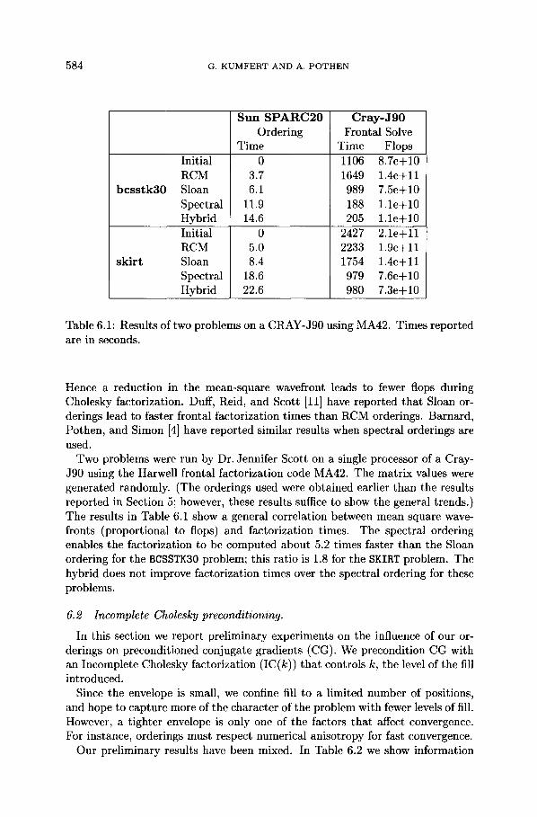
Hence a reduction in the mean-square wavefront leads to fewer flops during Cholesky factorization. Duff, Reid, and Scott [11] have reported that Sloan orderings lead to faster frontal factorization times than RCM orderings. Barnard, Pothen, and Simon [4] have reported similar results when spectral orderings are used.

Two problems were run by Dr. Jennifer Scott on a single processor of a Cray- J90 using the Harwell frontal factorization code MA42. The matrix values were generated randomly. (The orderings used were obtained earlier than the results reported in Section 5; however, these results suffice to show the general trends.) The results in Table 6.1 show a general correlation between mean square wavefronts (proportional to flops) and factorization times. The spectral ordering enables the factorization to be computed about 5.2 times faster than the Sloan ordering for the BCSSTK30 problem; this ratio is 1.8 for the SKIRT problem. The hybrid does not improve faztorization times over the spectral ordering for these problems.

6.2 Incomplete Cholesky preconditioning.

In this section we report preliminary experiments on the influence of our orderings on preconditioned conjugate gradients (CG). We precondition CG with an Incomplete Cholesky factorization (IC(k)) that controls k, the level of the fill introduced.

Since the envelope is small, we confine fill to a limited number of positions, and hope to capture more of the character of the problem with fewer levels of fill. However, a tighter envelope is only one of the factors that affect convergence. For instance, orderings must respect numerical anisotropy for fast convergence.

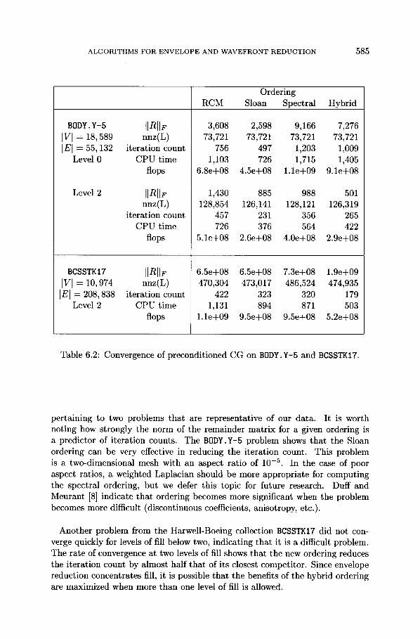
Our preliminary results have been mixed. In Table 6.2 we show information


BODY. Y-5

IVI = 18,589 IEI = 5 5 , 1 3 2

Level 0

Level 2

IIRIIF nnz(L)

iteration count CPU time

flops

IIRIIF nnz(L)

iteration count CPU time

flops

BCSSTK17 IIRIIF iVI = 10,974 nnz(L) IEI = 208,838 iteration count

Level 2 CPU time flops

Ordering RCM Sloan Spectral Hybrid

3,608 2,598 9,166 7,276 73,721 73,721 73,721 73,721

756 497 1,203 1,009 1,103 726 1,715 1,405

6.8e+08 4.5e+08 1.1e+09 9.1e+08

1,430 885 988 501 128,854 126,141 128,121 126,319

457 231 356 265 726 376 564 422

5.1e+08 2.6e+08 4.0e+08 2.9e+08

6.5e+08 6.5e+08 7.3e+08 1.9e+09 470,304 473,017 486,524 474,935

422 323 320 179 1,131 894 871 503

1.1e+09 9.5e+08 9.5e+08 5.2e+08

Table 6.2: Convergence of preconditioned CG on BODY.Y-5 and BCSSTK17.

pertaining to two problems that are representative of our data. It is worth noting how strongly the norm of the remainder matrix for a given ordering is a predictor of iteration counts. The BODY. Y-5 problem shows that the Sloan ordering can be very effective in reducing the iteration count. This problem is a two-dimensional mesh with an aspect ratio of 10 -5. In the case of poor aspect ratios, a weighted Laplacian should be more appropriate for computing the spectral ordering, but we defer this topic for future research. Duff and Meurant [8] indicate that ordering becomes more significant when the problem becomes more difficult (discontinuous coefficients, anisotropy, etc.).

Another problem from the Harwell-Boeing collection BCSSTKI7 did not con- verge quickly for levels of fill below two, indicating that it is a difficult problem. The rate of convergence at two levels of fill shows that the new ordering reduces the iteration count by almost half that of its closest competitor. Since envelope reduction concentrates fill, it is possible that the benefits of the hybrid ordering are maximized when more than one level of fill is allowed.


7 Conc lus ions .

We have observed that problems fall into two distinct classes when we examine how envelope parameters vary asymptotically as a function of the weights in the Sloan algorithm. Small wavefronts are obtained for the first class of problems when the the "local" term in the priority function is weighted large relative to the "global" term; for the second class of problems, the "global" term should be weighted to be more important. The bandwidth behaves contrary to the other envelope parameters for the first class, but its behavior is similar to the others for the second class. This is understandable since the bandwidth is a global property of an ordering of a graph.

A new normalized scheme for choosing weights according to the problem class improves the quality of the orderings computed by the Sloan algorithm. Our efficient implementation of the Sloan algorithm on the average required only 2.1 times the time taken by RCM, while producing mean square wavefronts about three times smaller than those obtained from RCM. Since the cost of the RCM algorithm is a few breadth-first-searches through the graph, these results imply that the Sloan algorithm is an effective combinatorial algorithm for computing envelope and wavefront reducing orderings.

Our modified Sloan algorithm for compressed graphs is very fast on problems that exhibit good compression. Since this algorithm mimics the computations that would be performed on the original unweighted graph, the faster algorithm does not sacrifice the quality of the orderings.

We have also described a hybrid algorithm that combines a spectral algorithm with a refinement step using a modified Sloan algorithm. The hybrid algorithm further improves the good envelope and wavefront reducing properties of the spectral algorithm. It produces orderings of better quality (about 60% of the mean square wavefront of normalized Sloan) but at a cost greater by a factor of five than the Sloan algorithm. In applications such as frontal factorization schemes, where the time taken to compute an ordering is insignificant relative to the subsequent factorization step, or for nonlinear problems where the cost of the ordering can be amortized over several linear solves, the hybrid algorithm is an attractive choice. However, in other applications where the tradeoff between the quality of the ordering versus the time required for computing the ordering favors fast ordering algorithms, the Sloan algorithm is attractive.

In this work we have primarily focused on improving the quality and time requirements of the Sloan algorithm. With similar attention to the eigencom- putation of the spectral algorithm we believe that the time requirements of the spectral algorithm could be reduced, and thereby the hybrid algorithm could be made more competitive. An interesting question is whether one can design algorithms that compute orderings with the same quality as the hybrid but at the cost of the Sloan algorithm. Boman and Hendrickson [5] have recently described an attempt in this direction, a multilevel algorithm for wavefront reduction.

Much more work is needed to understand the influence of these orderings .on the convergence behavior of preconditioned iterative solvers.

Our software implementing these algorithms is available with three different


interfaces: a stand-alone code, a code that can be called within Matlab, and another callable within PETSc. These codes are available from us upon request by electronic mail.

Acknowledgments

We thank Dr. Jennifer A. Scott of the Department of Computation and In- formation of Rutherford Appleton Laboratory for testing our orderings on the frontal code MA42, and Dr. Bruce Hendrickson of Sandia National Labs for modifying some of the Chaco functions to help us obtain accurate timing results. We are grateful to Dr. Scott and to Dr. Cleve Ashcraft (Boeing Information Services) for two rounds of careful reviews. Thanks also to Dr. Steve Guattery (ICASE) for comments on drafts of this paper.

REFERENCES

1. Anonymous, Harwell Subroutine Library, A Catalogue of Subroutines (Release 12). 1995.

2. C. C. Ashcraft, Compressed graphs and the minimum degree algorithm, SIAM J. Sci. Comput., 16 (1995), pp. 1404-1411.

3. J. E. Atkins, E. G. Boman, and B. Hendrickson, A spectral algorithm for the seriation problem. Tech. Report, Sandia National Lab, Albuquerque, NM.

4. S. T. Barnard, A. Pothen, and H. D. Simon, A spectral algorithm for envelope reduction of sparse matrices, J. Numerical Linear Algebra with Applications, 2 (1995), pp. 317-334. A shorter version has appeared in Supercomputing '93, IEEE Computer Society Press, pp. 493-502, 1993.

5. E. G. Boman and B. Hendrickson, A multilevel algorithm for envelope reduction, Preprint, Sandia National Labs, Albuquerque, NM, 1996.

6. E. H. Cuthill and J. McKee, Reducing the bandwidth of sparse symmetric matrices, in Proceed. 24th Nat. Conf. Assoc. Comput. Mach., ACM Publications, 1969, pp. 157-172.

7. E. F. D'Azevedo, P. A. Forsyth, and W. P. Tang, Ordering methods/or preconditioned conjugate gradients methods applied to unstructured grid problems, SIAM J. Matrix Anal. Appl., 13 (1992), pp. 944-961.

8. I. Duff and G. Meurant, The effect of ordering on preconditioned conjugate gradients, BIT, 29 (1989), pp. 635-657.

9. I. S. Duff, A. M. Erisman, and J. K. Reid, Direct Methods/or Sparse Matrices, Clarendon Press, Oxford, 1986.

10. I. S. Duff, R. G. Grimes, and J. G. Lewis, Users' Guide for the Harwell-Boeing Sparse Matrix Collection, 1992.

11. I. S. Duff, J. K. Reid, and J. A. Scott, The use of profile reduction algorithms with a frontal code, Internat. J. Numer. Meth. Engrg., 28 (1989), pp. 2555-2568.

12. M. Fiedler, Algebraic connectivity of graphs, Czechoslovak Math. J., 23 (1973), pp. 298-305.

13. M. Fiedler, A property of eigenvectors of nonnegative symmetric matrices and its application to graph theory, Czechoslovak Math. J., 25 (1975), pp. 619-633.

14. A. George, Computer implementation of the finite element method, Tech. Report 208, Department of Computer Science, Stanford University, Stanford, CA, 1971.


15. A. George and J. W-H. Liu, The evolution of the minimum degree algorithm, SIAM Review, 31 (1989), pp. 1-19.

16. A. George and A. Pothen, An analysis of spectral envelope-reduction via quadratic assignment problems, SIAM J. Matrix Anal. Appl., 18 (1997), pp. 706-732.

17. N. E. Gibbs, Algorithm 509: A hybrid profile reduction algorithm, ACM Trans. Math. Software, 2 (1976), pp. 378-387.

18. N. E. Gibbs, W. G. Poole, Jr., and P. K. Stockmeyer, An algorithm for reducing the bandwidth and profile of a sparse matrix, SIAM J. Num. Anal., 13 (1976), pp. 236-249.

19. J. R. Gilbert, G. L. Miller, and S.-H. Teng, Geometric mesh partitioning: Imple- mentation and experiments, Tech. Report CSL-94-13, Xerox Palo Alto Research Center, CA, 1994.

20. D. S. Greenberg and S. C. Istrail, Physical mapping with STS hybridization: oppor- tunities and limits, Tech. Report, Sandia National Labs, Albuquerque, NM, 1994.

21. R. G. Grimes, D. J. Pierce, and H. D. Simon, A new algorithm for finding a pseu- doperipheral node in a graph, SIAM J. Math. Anal. Appl., 11 (1990), pp. 323-334.

22. S. Guattery and G. Miller, On the performance of spectral graph partitioning methods, in 6th ACM-SIAM Symposium on Discrete Algorithms, San Francisco, 1995, ACM-SIAM, pp. 233-242.

23. C. Helmberg, B. Mohar, S. Poljak, and F. Rendl, A spectral approach to bandwidth and separator problems in graphs. Preprint, Department of Mathematics, University of Ljubljana, Lubljana, Slovenia, 1993.

24. B. Hendrickson and R. Leland, The Chaco User's Guide, Sandia National Labora- tories, Albuquerque, NM, 1993.

25. B. Hendrickson and R. Leland, A multilevel algorithm for partitioning graphs, Tech. Report SAND 93-0074, Sandia National Laboratories, Albuquerque, NM, 1993.

26. B. Hendrickson and R. Leland, An improved spectral graph partitioning algorithm .for mapping parallel computations, SIAM J. Sci. Comput., 16 (1995), pp. 452-469.

27. M. Juvan and B. Mohar, Laplace eigenvalues and bandwidth-type invariants of graphs. Preprint, Department of Mathematics, University of Ljubljana, Ljubljana, Slovenia, 1990.

28. M. Juvan and B. Mohar, Optimal linear labelings and eigenvalues of graphs, Discr. Appl. Math., 36 (1992), pp. 153-168.

29. J. G. Lewis, Implementations of the Gibbs-Poole-Stockmeyer and Gibbs-King algorithms, ACM Trans. Math. Software, 8 (1982), pp. 180-189.

30. Y. Lin and J. Yuan, Minimum profile of grid networks in structure analysis. Preprint, Department of Mathematics, Zhengzhou University, Zhengzhou, Henan 450052, People's Republic of China, 1993.

31. Y. Lin and J. Yuan, Profile minimization problem.for matrices and graphs. Preprint, Department of Mathematics, Zhengzhou University, Zhengzhou, Henan 450052, People's Republic of China, 1993.

32. J. W-H. Liu, A generalized envelope method for sparse faetorization by rows, Tech. Report CS-88-09, Department of Computer Science, York University, 1988.

33. J. W-H. Liu and A. H. Sherman, Comparative analysis of the CuthiU-Mekee and the reverse Cuthill-Mckee ordering algorithms for sparse matrices, SIAM J. Numer. Anal., 13 (1976), pp. 198-213.


34. G. L. Miller, S. H. Teng, W. Thurston, and S. A. Vavasis, Automatic mesh partitioning, in Graph Theory and Sparse Matrix Computation, A. George, J. R. Gilbert, and J. W-H. Liu, eds., The IMA Volumes in Mathematics and its Applications, 56, Springer-Verlag, pp. 57-84.

35. G. H. Paulino, I. F. M. Menezes, M. Gattass, and S. Mukherjee, Node and element resequencing using the Laplacian of a finite element graph, Part I, Internat. J. Numer. Meth. Engrg., 37 (1994), pp. 1511-1530.

36. G. H. Paulino, I. F. M. Menezes, M. Gattass, and S. Mukherjee, Node and element resequencing using the Laplacian of a finite element graph, Part II, lnternat. J. Numer. Meth. Engrg., 37 (1994), pp. 1531-1555.

37. A. Pothen, H. D. Simon, and K. P. Liou, Partitioning sparse matrices with eigenvectors of graphs, SIAM J. Matrix Anal. Appl., 11 (1990), pp. 430-452.

38. A. Pothen, H. D. Simon, and L. Wang, Spectral nested dissection, Tech. Report CS-92-01, Computer Science, Pennsylvania State University, University Park, PA, 1992.

39. S. W. Sloan, An algorithm for profile and wave/ront reduction of sparse matrices, Internat. J. Numer. Meth. Engrg., 23 (1986), pp. 239-251.

40. L. Wang, Spectral Nested Dissection, PhD thesis, The Pennsylvania State Univer- sity, 1994.

A T i m e C o m p l e x i t y

In this Appendix we analyze the computational complexity of the two Sloan implementations. The analysis has the interesting feature that the time complexity depends on the maximum wavefront size, a quantity related to the mean square wavefront that the algorithm is seeking to reduce. Nevertheless, it is possible to get a priori complexity bounds for problems with good separators. The results clearly show the overwhelming superiority of the heap implementation; an analysis of the complexity of the Sloan algorithm is not available in earlier published work.

The major computational difference lies in the implementation of the priority queue (see Section 3.2). We call these two implementations ArraySloan and HeapSloan according to the data structure used to implement the queue.

For the array implementation, the queue operations delete () , insert () , and i n c r e m e n t _ p r i o r i t y ( ) are all O(1) operations, but the m a x _ p r i o r i t y ( ) op- eration (finding the vertex with the maximum priority) is O(m), where m is the size of the queue. All operations on the binary heap are O(logm) except m a x _ p r i o r i t y ( ) , which is O(1).

To continue with our analysis, we will refer to the algorithm as shown in Fig- ure 3.1. It is immediately clear that the function f a r _ n e i g h b o r s ( ) (lines 26- 29) is O(deg(j)) for ArraySloan. We can bound this by A ---- maxl<i_<n(deg(i)). Similarly, f a r ne ighbors () for HeapSloan is O ( A . log m), where m is the maximum size of the priority queue.

The Sloan function (lines 1-25) has three loops: the initialization loop (lines 1-4), the outer ordering loop (lines 6-25), and the inner ordering loop (lines 9- 23). The initialization loop is the same for either implementation, and is easily seen to require O(IEI) time.


Consider now the ArraySloan implementation. For each step of the outermost loop starting at line 6, it must find and remove the vertex of maximum priority, requiring O(m) time. The inner loop is executed at most A times. The worst case for the inner loop is when the priority is incremented and the f a r neighbors routine is called, and this requires O(A) time. Thus the worst case running time for the ordering loop is O([V[ * (m + A2)). For the entire algorithm it is O([VI * (m + A 2) + IEI).

For the HeapSloan implementation, at each step of the outermost loop starting at line 6, the algorithm must delete the vertex of maximum priority, and then rebuild the heap; this takes O(log m) time. The inner loop is executed at most A times. The worst case for the inner loop is when the priority is incremented and the fa r_ne ighbors function is called. This time is O(A �9 logm). The worst case time complexity for the ordering loop of HeapSloan is thus O(IV I * A 2 * log m). For the entire algorithm it is O([V[ �9 A 2 * logm + [El).

These bounds can be simplified further. The maximum size of the queue can be bounded by the smaller of (1) the product of the maximum wavefront of the reordered graph and the maximum degree, and (2) the number of vertices n. Then the complexity of ArraySloan is O(]V I *A*maxwf), while the complexity of HeapSloan is O (I V I* A 2, log(maxwf, A) ). If we consider degree-bounded graphs, as finite element or finite difference meshes tend to be, then the ArraySloan implementation has time complexity O(IV [ �9 maxwf + IEI), while the HeapSloan implementation has O([V[ * log(maxwf) + IE]).

These bounds have the unsatisfactory property that they depend on the maximum wavefront, a quantity that the algorithm seeks to compute and to reduce. However, it is possible to remove this dependence from the bounds for important classes of finite element meshes, as we illustrate now.

The class of d-dimensional overlap graphs (where d _> 2) whose degrees are bounded includes finite element graphs with bounded aspect ratios embedded in d dimensions and all planar graphs [34]. Overlap graphs have O(n (d-1)/d) separators that split the graph into two parts with the ratio of their sizes at most (d + 1)/(d + 2). Hence the maximum wavefront can be bounded by O(n (d-1)/d) for a modified nested dissection ordering that orders one part first, then the separator, and finally the second part. The Sloan and other envelope-reducing algorithms tend to do better than this modified nested dissection ordering, so we can assume that the maximum wavefront for the Sloan algorithm is also bounded by this bound.

With the above assumption, we can conclude that the HeapSloan implementation requires O(nlogn) time while the ArraySloan implementation requires O(n (2d-1)/d) time for a d-dimensional overlap graph. For a planar mesh (d = 2), the ArraySloan implementation requires O(n 3/2) time, while for a three dimensional mesh with bounded aspect ratios (d = 3), its time complexity is 0(n5/3).

Documents

Two improved algorithms for envelope and wavefront reduction