Two-dimensional Hurst-Kolmogorov process and its application to rainfall fields

Demetris Koutsoyiannis1, Athanasios Paschalis

1,2 and Nikos Theodoratos

1

1. Department of Water Resources and Environmental Engineering, Faculty of Civil

Engineering, National Technical University of Athens, Heroon Polytechneiou 5, GR-157 80

Zographou, Greece

2. Institute of Environmental Engineering, ETH - Swiss Federal Institute of Technology, ETH

Hönggerberg, HIF CO 46.8, CH - 8093 Zürich, Switzerland

Corresponding author: D. Koutsoyiannis, dk@itia.ntua.gr

Abstract The Hurst-Kolmogorov (HK) dynamics has been well established in stochastic

representations of the temporal evolution of natural processes, yet many regard it as a puzzle

or a paradoxical behaviour. As our senses are more familiar with spatial objects rather than

time series, understanding the HK behaviour becomes more direct and natural when the

domain of our study is no longer the time but the two-dimensional space. Therefore, here we

detect the presence of HK behaviour in spatial hydrological and generally geophysical fields

including Earth topography, and precipitation and temperature fields. We extend the one-

dimensional HK process into two dimensions and we provide exact relationships of its basic

statistical properties and closed approximations thereof. We discuss the parameter estimation

problem, with emphasis on the associated uncertainties and biases. Finally, we propose a two-

dimensional stochastic generation scheme, which can reproduce the HK behaviour and we

apply this scheme to generate rainfall fields, consistent with the observed ones.

Keywords Hurst-Kolmogorov dynamics; stochastic processes; stochastic simulation; random

fields; rainfall fields; hydrometeorology

2

1. Introduction

Very few people know the beauty of the mountains (Osho)

In his seminal paper, H. E. Hurst (1951), after studying numerous geophysical time series,

observed that: “Although in random events groups of high or low values do occur, their

tendency to occur in natural events is greater. This is the main difference between natural and

random events”. This difference triggered coining the term “Hurst phenomenon”, which even

today many regard as an enigma or a puzzle, as also implied by the denotation “phenomenon”

in this term. Koutsoyiannis and Cohn (2008) tried to show that the reluctance to recognize this

behaviour and incorporate it into standard geophysical statistics may be related to the

unfavourable terminology used, including “phenomenon” and the related term “long memory”

introduced by the influential studies by Mandelbrot and Wallis (1968) and Mandelbrot and

van Ness (1968). Specifically, “long memory” (a metaphoric term related to slowly decaying

autocorrelation) gives a wrong message leading to incorrect understanding of the physical

mechanism. “Long memory” is counterintuitive and not realistic. Klemes (1974) insisted that

“the Hurst phenomenon is not necessarily an indicator of infinite memory of a process” and

pointed out that it can be explained in terms of long-term change rather than long-term

memory. He also compared the memory-based interpretation to the Ptolemaic planetary

model, which worked well but hampered progress in astronomy for centuries. Koutsoyiannis

(2002) demonstrated that changes occurring at multiple (e.g. three or more) time scales result

in a process exhibiting Hurst behaviour and Koutsoyiannis (2005b) showed that the same

process can be derived by applying the principle of maximum entropy (i.e., uncertainty) on

multiple time scales. Following Koutsoyiannis and Cohn (2008) and to give proper credit to

A. N. Kolmogorov (1940), who was the first to propose a mathematical model to describe this

behaviour (for the study of turbulence), here we refer to this behaviour as the Hurst-

Kolmogorov (HK) behaviour and to the stationary stochastic process that reproduces it as the

HK process.

As our senses are more familiar with spatial objects rather than time series, the

understanding of the HK behaviour becomes more direct and natural when the domain in

3

which we study a geophysical process is no longer the time but the two-dimensional (2D)

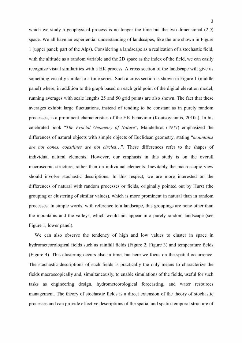
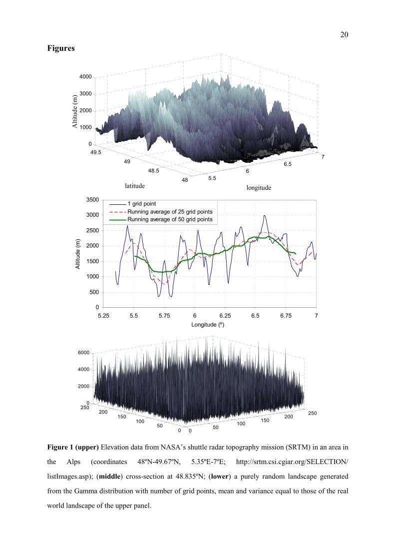
space. We all have an experiential understanding of landscapes, like the one shown in Figure

1 (upper panel; part of the Alps). Considering a landscape as a realization of a stochastic field,

with the altitude as a random variable and the 2D space as the index of the field, we can easily

recognize visual similarities with a HK process. A cross section of the landscape will give us

something visually similar to a time series. Such a cross section is shown in Figure 1 (middle

panel) where, in addition to the graph based on each grid point of the digital elevation model,

running averages with scale lengths 25 and 50 grid points are also shown. The fact that these

averages exhibit large fluctuations, instead of tending to be constant as in purely random

processes, is a prominent characteristics of the HK behaviour (Koutsoyiannis, 2010a). In his

celebrated book “The Fractal Geometry of Nature”, Mandelbrot (1977) emphasized the

differences of natural objects with simple objects of Euclidean geometry, stating “mountains

are not cones, coastlines are not circles…”. These differences refer to the shapes of

individual natural elements. However, our emphasis in this study is on the overall

macroscopic structure, rather than on individual elements. Inevitably the macroscopic view

should involve stochastic descriptions. In this respect, we are more interested on the

differences of natural with random processes or fields, originally pointed out by Hurst (the

grouping or clustering of similar values), which is more prominent in natural than in random

processes. In simple words, with reference to a landscape, this groupings are none other than

the mountains and the valleys, which would not appear in a purely random landscape (see

Figure 1, lower panel).

We can also observe the tendency of high and low values to cluster in space in

hydrometeorological fields such as rainfall fields (Figure 2, Figure 3) and temperature fields

(Figure 4). This clustering occurs also in time, but here we focus on the spatial occurrence.

The stochastic descriptions of such fields is practically the only means to characterize the

fields macroscopically and, simultaneously, to enable simulations of the fields, useful for such

tasks as engineering design, hydrometeorological forecasting, and water resources

management. The theory of stochastic fields is a direct extension of the theory of stochastic

processes and can provide effective descriptions of the spatial and spatio-temporal structure of

4

hydrometeorological fields. In particular, for the rainfall fields, whose study is crucial for the

rational design of flood protection works and the flow hydrograph prediction in real time,

specialized models, e.g. based on the extension of point processes to spatial structures (e.g.

Chandler et al., 2002) have been developed and effectively used. A more generalized

framework for studying geophysical fields has been provided by the notion of multifractals

(e.g. Schertzer and Lovejoy, 1987; Lovejoy and Schertzer, 1995; Pathirana and Herath, 2002;

Gagnon et al., 2006; Veneziano and Langousis, 2010; Koutsoyiannis and Langousis, 2011),

which has given impressive and operational results for the characterization and stochastic

simulation of natural fields such as rainfall, cloud structure and Earth topography.

However, here we prefer to use the simpler notion of a 2D HK process (see e.g. Penttinen

and Virtamo, 2003), which is a direct extension in a 2D space of the well-known 1D HK

process (also known as fractional Gaussian noise—fGn, due to Mandlbrot and van Ness,

1968), based on the formalism that Kolmogorov and later (independently) Mandelbrot

proposed. In fact the 2D HK process, which we describe next, is the simplest stochastic

process that represents the above described natural behaviour. Its simplicity is a valuable

characteristic when understanding is a principal target, and is also associated with parsimony

of parameterization and mathematical ease: it uses a single parameter, the Hurst coefficient H,

additional to those of classical statistics. Simplicity and parsimony make it realistic to derive

all mathematical properties and also produce a full stochastic simulation model by easy

analytical means.

This formalism has some additional advantages over some multifractal studies. Thus, it

distinguishes the different types of scaling behaviours, i.e. the scaling in state and the scaling

in time and/or space (Koutsoyiannis, 2005a), which some multifractal analyses confuse.

Specifically, the scaling in state is a property of the marginal (order 1) distribution function

(and here is handled using appropriate marginal distribution functions or appropriate

normalizing transformation of the random variable of interest) whereas the scaling in space

and time are properties characterizing the dependence structure of the field and are clearly

associated with different scaling exponents, with different meanings. Furthermore the HK

formalism allows understanding and characterizing the uncertainties and biases associated

5

with the estimation of the statistical properties and parameters of the process or field. As we

will see next, such uncertainties and biases are prominent, substantially higher than in purely

random processes, even in the estimation of the lowest moments, such as means and standard

deviations. Some multifractal analyses miss this and do not properly account for the

uncertainty and bias. However, the enhancement of uncertainty is perhaps the most important

characteristic that a proper understanding of the scaling behaviour of nature should include.

Neglecting uncertainties and biases (as often done in multifractal studies that, for example,

rely on estimates of high order statistical moments treating them as if they were precisely

known quantities), may have dramatic consequences at all modelling aspects including the

identification of the appropriate model (Koutsoyiannis, 2010b; Papalexiou et al., 2010).

2. Stochastic model

We denote by z a random variable representing the modelled quantity of interest (e.g.

topographic elevation, rainfall, temperature, or nonlinear transformations thereof) and by z

(without underscore) any realization (numerical value) of the variable. We assume that z is

defined on a 2D space denoted by the continuous (real) variables (x, y) or the discrete

(integer) variables (i, j) which define the index space of the stochastic field z(x, y) or zi,j; the

two are related as

zi,j := 1

∆2 ⌡⌠

(i – 1)∆

i ∆

⌡⌠(j – 1)∆

j ∆

z(x, y) dx

dy (1)

where ∆ is a fixed interval representing a “unit” scale for conversion of continuous to discrete

spatial representation. The discrete space representation has several advantages, both practical

(simulations are necessarily done in gridded space) and theoretical (as we will see, the

continuous space representation involves some infinities). Therefore our analysis will be

based on discretized space, while we will use the continuous-space representation in an

auxiliary role. For simplicity and in accord to the explanatory character of this study, we

assume that the field z is stationary and isotropic and we denote its mean as µ := E[zi,j], its

autocovariance as γk,l := Cov[zi,j, zi+k,j+l] and its autocorrelation as ρk,l := Corr[zi,j, zi+k,j+l] =

γk,l/γ0, where γ0 is the variance, i.e. γ0 := Var[zi,j] = γ0,0 ≡ σ2 (σ denotes standard deviation).

6

Furthermore we define the average process at a spatial scale which is an integer (k = 1, 2,

…) multiple of ∆, i.e.,

z(k)i,j :=

1

k2 ∑

m=(i–1)k+1

ik

∑n=(j–1)k+1

jk

zm,n (2)

and denote its autocovariance as γ(k)l,m , its variance as γ

(k)0 and its autocorrelation as ρ

(k)l,m . The

notation implies that a superscript equal to 1 can be omitted (i.e., z(1)i,j ≡ z

i,j , γ

(1)l,m ≡ γ

l,m , etc.).

A 2D HK process can be defined as a stochastic process, which for any indices i, j, m, n,

and any scales k and l, has the property

(z(k)i,j – µ) =d

k

l

2H – 2

(z(l)m,n – µ) (3)

where =d means that the two random variables have the same finite-order joint distribution

functions. The constant H in the exponent is the so called Hurst coefficient and takes on

values in the interval (0, 1). Setting l = 1 in (3) and taking variances, we easily obtain that the

variance at scale k is

γ(k)0 = k 4H – 4

γ0 (4)

For comparison, we recall that in the standard, 1D, HK process, defined by

(z(k)i – µ) =d

k

l

H – 1

(z(l)m – µ) (5)

the variance at scale k is

γ(k)0 = k

2H – 2 γ0 (6)

In the 1D case, the autocorrelation function can be easily derived from (5) and is

ρj = g1(j; H) := |j + 1|2H

/ 2+ |j – 1|2H

/ 2 – |j|2H

≈ H(2H – 1) |j|2H–2

(7)

where j is the lag. This however, is more difficult to determine in the 2D process. Initially,

similar to the 1D process, we can observe that (3) defines three very different types of

processes. Specifically, for H = 0.5, it can be easily verified that (4) characterizes a purely

random process with zero autocorrelation. For 0 < H < 0.5, it can be demonstrated from (4)

(e.g., for scales 1 and 2) that the autocorrelation is negative even for the smallest

7

displacements or lags (e.g. a displacement equal to one). While this is mathematically

possible and describes a special type of an antipersistent process, it is not physically realistic:

Consistency with physical reality demands that at neighbouring times or locations the process

should be positively correlated (Koutsoyiannis, 2010a). Finally, the case 0.5 < H < 1 defines a

physically realistic process which has the clustering or grouping behaviour discussed in the

Introduction. For the latter case, for the continuous space representation of a stationary and

isotropic process we can write the autocovariance function as

γ(lx,ly) := Cov[z(x, y), z(x + lx, y + ly)] = f(r) = f( lx

2 + ly

2 ) (8)

where lx and ly denote spatial displacements in the directions x and y, respectively, f is a

function to be specified and r := lx

2 + ly

2 is the radial displacement. As shown in Appendix

A, a specific form of the function f(r) consistent with (4) is

f(r) = a r 4H – 4 (9)

where a is any constant. Based on this, in Appendix A we derive the exact variance as a

function of H and the autocorrelation function for the discrete space representation, which is

most useful in applications. These functions do not have a closed form. Nonetheless, simple

closed approximations are possible and are derived in Appendix A from numerical solutions,

i.e.,

γ(k)0 ≈

3 a

(2H – 1) (4H – 1) k4H – 4 ∆ 4H – 4 (10)

ρ(k)l,m ≈ ρ

(k)d = g2(d; H) := min

(4 H – 1)[g1(d; H)]

2

3H2 (2H – 1)

, g1(d; H) (11)

where d = l2 + m

2 is the radial displacement in the discrete space representation

corresponding to spatial displacements in the directions x and y equal to l and m, respectively

(notice that d is not necessarily an integer, even if l and m are, but (11) can be applied even

for non-integer d, l and m). It is seen in Figure 5 that the approximations of the variance γ(k)0 by

(10) (upper panel) and the autocorrelation ρ(k)l,m by (11) are very good for all values of H and

all displacements. A further simplification of (11) can be obtained by observing that the two

terms in the curly brackets in (11) become almost equal for d = 1 and thus

8

ρ(k)d ≈ min

[g1(d; H)]

2

g1(1; H), g1(d; H) = g1(d; H) min

g1(d; H)

g1(1; H), 1 (12)

Comparing the continuous-space with the discrete-space representation, we can observe

that in the former the variance (obtained from f(r) in (9) for r = 0) is infinite, whereas in the

latter it is always finite (tending to infinity as the scale k → 0). In addition, in the continuous-

space representation the autocorrelation function cannot be defined (because the variance is

infinite), whereas in the discrete-space representation, not only can be it defined, but it is

invariant for any scale and thus is the most characteristic function of the stochastic field.

The spectral density scγ(ux, uy) of the stochastic field (where ux and uy are frequencies at the

two directions) for the continuous space representation is presented in Appendix A and can

also provide an approximation of the spectral density for the discrete space representation,

which is a power function of the radial frequency p := ux

2 + uy

2, i.e.,

sγ(ux, uy) = sγ(p) = c p2 – 4H (13)

where c depends on the variance γ0 and the Hurst parameter H.

3. Parameter estimation

We assume that the observed sample zi,j extends over a rectangular area with edge size km, and

we regard zi,j as a realization of the HK field zi,j. The sample size is n = k2m. Using the notation

of section 2, the sample average is, clearly, z– ≡ z(km)1‚1 . It can be readily shown that z– is an

unbiased estimator of the mean µ in HK statistics (HKS) as in classical statistics (CS) in

which the sample is random, i.e. all its elements are independent and identically distributed

(iid). By virtue of (4), the variance of the estimator of z– is

Var[z–] = σ

2

n2 – 2H (14)

which is identical to that in the 1D HK process but, for high H, departs notoriously from the

corresponding law in classical statistics, i.e.,

Var[z–] = σ

2

n (15)

The latter equation can be written as n = σ2/Var[z–] and, by analogy, this allows us to define an

“equivalent” or “effective” sample size n΄ of an HKS sample of size n, such that a sample size

9

n΄ in CS results in the same uncertainty of the mean as a sample with size n in HKS.

Specifically, we define

n΄ := σ2/Var[z–]

(16)

so that for an HK process

n΄ = n2 – 2H

(17)

The estimator of the variance in CS is

s2 =

1

n – 1 ∑i = 1

k

∑j = 1

k

(zi,j – z–)2

(18)

(with s standing for standard deviation) and is unbiased for independent zi,j. For dependent zi,j,

it can be easily inferred that the expected value of s2 is

E[s2] =

n

n – 1 {E[z

2i,j ] – E[z–

2]} =

n

n – 1 {Var[z

i,j ] – Var[z–]}

(19)

or

E[s2] =

1 – 1/n΄

1 – 1/n σ

2 (20)

This indicates that the classical estimator is biased. The bias may be very high for high H: for

example, for H = 0.99 (and, as we will see below, this value is not unrealistically high) and

for k = 100, so that n = k2 = 10 000, n΄ = 1.20 (only!), so that E[s

2] = 0.17 σ

2 (a 83% bias!).

Notably, equations (17) and (20) are precisely the same as in the 1D HK process

(Koutsoyiannis, 2003; Koutsoyiannis and Montanari, 2007).

The parameters σ and H are dependent to each other, whereas µ is independent to both

(Tyralis and Koutsoyiannis, 2010). Thus, µ can be easily estimated by z–. However, the

estimation of σ and H should be done simultaneously and should take into account the bias in

the estimation of standard deviation. Here we follow an algorithm similar to that proposed by

Koutsoyiannis (2003) for the 1D HK process, which is based on the CS estimates s(k)

at

several scales k from k = 1 to a maximum scale k΄ chosen such that the sample size nk΄ at that

scale is at least 10. In the 2D case, the edge length at scale k is [km/k] (where the square

brackets denote the integer part of a real number), so that nk = [km/k]2.

From (20) we obtain

E[(s(k)

)2] =

1 – 1/n΄k

1 – 1/nk (σ

(k))2

(21)

10

or, combining (4) and (17),

E[(s(k)

)2] = ck(H) k

4H – 4 σ

2 (22)

where ck(H) := (1 –

1/n΄k)

/ (1

–

1/nk)

= (1

–

[k/km]

4 – 4H) / (1

–

[k/km]

2) is a bias correction factor.

Therefore, we try to minimize the fitting error of the estimated variance (s(k)

)2 to the right-

hand side of (22), as detailed in Appendix B.

Equation (22), which is the basis of this method of parameter estimation, has an easy

graphical depiction, which is very useful to assess whether the HK model is appropriate or

not. This is made by a logarithmic plot of the estimated variance (s(k)

)2 (or the estimated

standard deviation s(k)

) versus scale k, also known as climacogram (from the Greek climax,

meaning scale; Koutsoyiannis, 2010a). In a purely random (iid) process, where H = 0.5, the

double logarithmic plot of (s(k)

)2 vs. k will form a straight line with slope –2. In a positively

autocorrelated HK process, if we plot the true (population) variance γ(k)0 ≡ (σ

(k))2, as given in

(4), not considering the bias correction factor ck(H), we will have a straight line with a milder

slope, 4H – 4. However, because for large H the factor ck(H) is significantly lower than 1 and

cannot be neglected, the plot of E[(s(k)

)2] given in (22) vs. k would be a concave curve, with

slope becoming steeper as k increases. The plot of the sample estimate of variance (s(k)

)2

should comply with that of E[(s(k)

)2] rather than with that of γ

(k)0 .

Figure 6 depicts such climacograms for the example fields discussed above and given in

Figures 1-4. The estimated parameters for all fields are shown in Table 1 and it can be seen

that in all cases the Hurst coefficient is exceptionally high (0.99 < H < 1). It is important that

H < 1, because in the case H = 1 the theoretical variance becomes infinite (even in the discrete

space representation), whereas the case H > 1 is mathematically meaningless. Figure 6 shows

that the HK framework provides a better alternative in modelling all examined examples, in

comparison to the classical, iid model, which is fully inappropriate.

4. Simulation scheme

A simple scheme for generation of realizations of the 2D HK process can be derived as an

extension of the 1D symmetric moving average (SMA) scheme, introduced by Koutsoyiannis

(2000), which is a stochastic model that can generate time series with any autocorrelation

11

structure. Extending the 1D scheme, we introduce the 2D SMA scheme as

zi,j = ∑l = –∞

∞

∑m = –∞

∞

αl,m vi–l,j–m (23)

where αl,m is a field of coefficients to be determined and vi,j is a discrete white noise random

field with zero mean and unit variance (assuming also, without loss of generality, that µ =

E[zi,j] = 0). Numerically, this can be implemented using a finite number (q) of coefficients,

i.e.,

zi,j = ∑l = –q

q

∑m = –q

q

αl,m vi–l,j–m (24)

By extending the 1D analysis in Koutsoyiannis (2000) it can be shown without difficulties

that the Fourier transform of the field α, sα(ux, uy) = sα(p), is related to that of the

autocovariance sγ(ux, uy) by

sα(ux, uy) = sγ(ux, uy) (25)

By virtue of (13),

sα(ux, uy) = c p1 – 2H (26)

Comparing (13) and (26), we observe that the latter is equivalent to the Fourier transform of

the autocovariance of a HK process with Hurst parameter H΄, so that 2 – 4H΄ = 1 – 2H or H΄ =

(0.5 + H)/2. By inverting the Fourier transform, we conclude that the coefficients αl,m should

be proportional to the autocorrelations ρl,m of an HK process with Hurst parameter H΄, i.e.,

αl,m = c΄ ρl,m = c΄ g2( l2 + m

2; 1/4 + H/2) (27)

where the function g2( ) is defined in (11) and c΄ is an unknown constant. The latter could be

determined by observing that (24) results in

γ0 = ∑l = –q

q

∑m = –q

q

α2l,m (28)

or

γ0 = c΄2 ∑l = –q

q

∑m = –q

q

[g2( l2 + m

2; 1/4 + H/2)]

2 (29)

which can be readily solved for c΄.

An example demonstration of the simulation scheme has been done for the rainfall field of

12

Figure 3. The model described above can easily generate Gaussian random fields. However,

the examined rainfall field (as well as several geophysical processes and fields) is not

Gaussian and, thus, we need to normalize the original field before applying the procedure.

Several families of transformations can be found in the bibliography, e.g., the Box-Cox

family of transformations (Box and Cox, 1964), which in many cases give satisfactory results.

However, this normalizing transformation is not appropriate for rainfall, because it produces

exponential distribution tails, while the rainfall distribution tails are more likely of power type

(Koutsoyiannis, 2004, 2005a), thus reflecting an asymptotic scaling behaviour in state.

Therefore, here we used the transformation

z = g(x) = λ

1 + x

ν

–θ

1 + 1

κ ln

1 + κ x

λ

2

(30)

which has a power-type tail. In (30), θ and κ are dimensionless parameters, and λ and ν are

parameters with dimensions identical to those of x, so that z has also dimensions identical to

those of x. This transformation is derived from a similar one introduced by Koutsoyiannis et

al. (2008), which aimed to produce a power-type right tail in the distribution of x. The

quantity [1 + (x/ν) –θ

] was proposed by Papalexiou et al. (2007) because it provides a better fit

on the left tail of the distribution of x. The parameters of the transformation are θ = 1.0715, κ

= 3.6016, λ = 3.0429 mm, ν = 1.7039 mm, and the normalized field is shown in Figure 3

(right).

The Hurst coefficient of the normalized field, is estimated, using the algorithm of

Appendix B, to H = 0.997. A normalized stochastic field generated using the above method is

shown in Figure 7 with statistical estimates given in Table 2, along with the de-normalized

(natural) synthetic rainfall field, obtained by inverting the transformation (30) (this can be

done only numerically). The comparison of the statistical characteristics of the synthetic field

with the original one of Figure 3 is given in Table 2 and Figure 7 and indicates a good

performance of the simulation algorithm.

13

5. Summary, conclusions and discussion

The so-called Hurst phenomenon, detected in many geophysical processes, has been regarded

by many as a puzzle. The “infinite memory”, often associated with it, has been regarded as a

counterintuitive and paradoxical property. However, it may be easier to perceive the Hurst-

Kolmogorov behaviour if one detaches the “memory” interpretation and associates it with the

rich patterns apparent in real world phenomena, which are absent in purely random processes.

Furthermore, as our senses are more familiar with spatial objects rather than time series,

understanding the Hurst-Kolmogorov behaviour becomes more direct and natural when the

domain, in which we study a geophysical process, is no longer the time but the 2D space. In

this respect, this study offers an extension of the one-dimensional HK process into two

dimensions. We provide exact relationships of its basic statistical properties and closed

approximations thereof. We discuss the parameter estimation problem, with emphasis on the

increased uncertainties and biases of the classical statistical estimators, when applied to a

Hurst-Kolmogorov process. These are very similar, as in the one-dimensional HK process.

Finally, we study a stochastic generation scheme, which can reproduce the HK behaviour.

The scheme is an extension of the symmetric moving average algorithm introduced by

Koutsoyiannis (2000), which can perform with any arbitrary autocorrelation function.

This study has an exploratory and explanatory character and, therefore, the focus is on the

simplest and most parsimonious, yet sufficiently realistic, representation of real world fields,

such as terrain, rainfall and temperature. It does not aim to provide detailed modelling tools

for such fields. Therefore, the stochastic model relies on a single parameter, the Hurst

coefficient, to describe the spatial dependence of the field. The assumption of homogeneous

and isotropic fields is, therefore, appropriate for the scope of this study, although in a more

detailed representation of natural fields it may be relaxed (e.g. to take account of the

dependence of precipitation intensity on altitude and geographical characteristics). Evidently,

further research is needed for the case where this assumption is relaxed.

Acknowledgment We thank Tim Cohn and another reviewer for their kind and encouraging

comments and their useful suggestions.

14

Appendix A: Exact statistical properties of the 2D HK process and derivation of

their approximations

Combining (1) and (8) we obtain that the discrete-space autocovariance is

γl,m = Cov[z1,1, z1+l,1+m] = 1

∆4 ⌡⌠

x = 0

∆

⌡⌠y = 0

∆

⌡⌠x΄ = l∆

(l + 1)∆

⌡⌠y΄ = m∆

(m + 1)∆

f( (x – x΄)2 + (y – y΄)

2) dxdydx΄dy΄ (A1)

After algebraic manipulations which are typical for stochastic processes, the above integral

can be reduced to a double integral, i.e.,

γl,m = ⌡⌠–1

1 ⌡⌠

–1

1 f(∆ (l – ξ)

2 + (m – ψ)

2) (1 – |ξ|) (1 – |ψ|)dξdψ (A2)

For l = m = 0, we obtain the variance of the process, i.e.

γ0 = ⌡⌠–1

1 ⌡⌠

–1

1 f(∆ ξ

2 + ψ

2) (1 – |ξ|) (1 – |ψ|)dξdψ (A3)

which obviously simplifies to

γ0 = 4 ⌡⌠0

1 ⌡⌠

0

1 f(∆ ξ

2 + ψ

2) (1 – |ξ|) (1 – |ψ|)dξdψ (A4)

Likewise, the variance at scale k is

γ(k)0 = 4 ⌡⌠

0

1 ⌡⌠

0

1 f(k∆ ξ

2 + ψ

2) (1 – |ξ|) (1 – |ψ|)dξdψ (A5)

It can be easily verified that a sufficient condition to make (A5) consistent with (4) is the one

given in (9). By virtue of (9), the discrete-space variance from (A4) for any spatial scale k∆

becomes

γ(k)0 = a k4H – 4 ∆ 4H – 4 I0(H) (A6)

where

I0(H) := 4⌡⌠0

1 ⌡⌠

0

1 (ξ

2 + ψ

2)2H – 2

(1 – |ξ|) (1 – |ψ|)dξdψ (A7)

Likewise,

γ(k)l,m = a k4H – 4 ∆ 4H – 4 Il,m(H) (A8)

15

where

Il,m(H) := ⌡⌠–1

1 ⌡⌠

–1

1 [(l – ξ)

2 + (m – ψ)

2]2H – 2

(1 – |ξ|) (1 – |ψ|)dξdψ (A9)

We observe that the quantity I0(H) depends only on the Hurst coefficient H, whilst Il,m(H)

depends also on the displacements l and m. The autocorrelation function is

ρ(k)l,m = Il,m(H) / I0(H) (A10)

and is independent of the scale k and the constant a.

The integral I0(H) has a rather complicated and inconvenient analytical expression whereas

Il,m(H) is difficult to express in a closed form. However, numerical integration is very easy

and, from its results, simple analytical approximations can be derived. Specifically, I0(H) can

be calculated as

I0(H) ≈ 3

(2H – 1) (4H – 1) (A11)

which allows the approximation of γ(k)0 given in (10).

For Il,m(H) we first observe that for l and m much larger than 1, the term in square brackets

in (A9) can be approximated as (l2 + m

2)2H – 2

, or d4H – 4

. Thus, it is easy to see that

Il,m(H) = Id(H) ≈ d4H – 4

, for d >> 1 (A12)

so that

ρ(k)l,m ≈ ρ

(k)d ≈ (1/3) (2H – 1) (4H – 1) d

4H – 4, for d >> 1 (A13)

For smaller values of d down to zero, we can make use of the function g1(d; H) that defines

the autocorrelation of the 1D process, to find an approximation valid for all displacements.

From (A13) and (7) we observe that, for high d, the autocorrelation ρd in the 2D case is

proportional to the square of ρd in the 1D case with proportionality coefficient equal to

[(1/3) (2H – 1) (4H – 1)] / [H(2H – 1)]2. We extend this proportionality to smaller d, also

disallowing the autocorrelation of the 2D case to exceed that of the 1D case. This results in

(11).

The spectral density scγ(ux, uy) of the stochastic field for its continuous-space representation

16

can be calculated by taking the 2D Fourier transform scγ(ux, uy) of the autocovariance γ(lx,ly) =

a (lx

2 + ly

2)2H – 2

. Due to circular symmetry (γ(lx,ly) = γ(r) = a r4H – 4

for r := lx

2 + ly

2), the 2D

Fourier transform equals the Henkel transform for the radial frequency p := ux

2 + uy

2

(Bracewell, 2000, p. 336), i.e.,

scγ(ux, uy) = s

cγ(p) = 2π ⌡⌠

0

∞

r γ(r) J0(2πpr) dr (A14)

where J0( ) is the Bessel function of the first kind. This results in

scγ(ux, uy) = s

cγ(p) = a π3 – 4H

Γ(2H – 1)

Γ(2 – 2H) p

2 – 4H (A15)

where Γ( ) is the gamma function. We can then conclude that an approximation of the spectral

density for the discrete space representation will also be a power function of the frequency p,

as given by (13).

Appendix B: Fitting error and its minimization

As stated, the basis of the fitting method is the minimization of the fitting error of the

estimated variance (s(k)

)2 to the right-hand side of (22). In logarithmic terms and using weights

equal to 1/k2 to the partial error of each scale k, the fitting error is

e2(σ, H) := ∑

k=1

k'

{ln[(s

(k))2] – ln[ck(H) k

4H – 4 σ

2]}

2

k2

(B1)

which, after algebraic manipulations, becomes

e2(σ, H)/4 = ∑

k=1

k'

[ln (k

2 s

(k)) – ln ck(H)/2 – H ln k

2 – ln σ]

2

k2

(B2)

The minimization of (B2) can be done only numerically and results in the optimal estimates

of σ and H simultaneously (see the algorithmic details in Koutsoyiannis, 2003, and Tyralis

and Koutsoyiannis, 2010).

17

References

Box, G. E. P. and D. R. Cox (1964) An analysis of transformations, Journal of the Royal Statistical

Society B, 26 (2), 211-252.

Bracewell, R. N. (2000) The Fourier Transform and Its Applications, 3rd Edition, McGraw-Hill,

Boston, Mass., USA.

Chandler, R. E., H. S. Wheater, V. S. Isham, C. Onof, S. M. Bate, P. J. Northrop, D. R. Cox, and D.

Koutsoyiannis (2002) Generation of spatially consistent rainfall data, Continuous river flow

simulation: methods, applications and uncertainties, BHS Occasional Paper No. 13, 59–65, British

Hydrological Society, London.

Gagnon, J.-S., S. Lovejoy, and D. Schertzer (2006) Multifractal earth topography, Nonlin. Processes

Geophys. 13, 541-570.

Hurst, H. E. (1951) Long term storage capacities of reservoirs, Trans. ASCE 116, 776-808.

Klemes, V. (1974) The Hurst phenomenon: A puzzle?, Water Resour. Res. 10 (4) 675-688.

Kolmogorov, A. N. (1940) Wienersche Spiralen und einige andere interessante Kurven in

Hilbertschen Raum, Dokl. Akad. Nauk URSS 26, 115–118.

Koutsoyiannis, D. (2000) A generalized mathematical framework for stochastic simulation and

forecast of hydrologic time series, Wat. Resour. Res. 36 (6), 1519-1534.

Koutsoyiannis, D. (2002) The Hurst phenomenon and fractional Gaussian noise made easy,

Hydrological Sciences Journal 47 (4), 573–595.

Koutsoyiannis, D. (2003), Climate change, the Hurst phenomenon, and hydrological statistics,

Hydrological Sciences Journal, 48(1), 3-24.

Koutsoyiannis, D. (2004) Statistics of extremes and estimation of extreme rainfall, 2, Empirical

investigation of long rainfall records, Hydrological Sciences Journal 49 (4), 591–610.

Koutsoyiannis, D. (2005a) Uncertainty, entropy, scaling and hydrological stochastics, 1, Marginal

distributional properties of hydrological processes and state scaling, Hydrological Sciences Journal

50 (3), 381–404.

Koutsoyiannis, D. (2005b) Uncertainty, entropy, scaling and hydrological stochastics, 2, Time

dependence of hydrological processes and time scaling, Hydrological Sciences Journal 50 (3),

405–426.

18

Koutsoyiannis, D. (2010a) A random walk on water, Hydrology and Earth System Sciences 14, 585–

601.

Koutsoyiannis, D. (2010b) Some problems in inference from time series of geophysical processes

(solicited), European Geosciences Union General Assembly 2010, Geophysical Research

Abstracts, Vol. 12, Vienna, EGU2010-14229, European Geosciences Union

(http://www.itia.ntua.gr/en/docinfo/973/).

Koutsoyiannis, D., and T. A. Cohn (2008) The Hurst phenomenon and climate (solicited), European

Geosciences Union General Assembly 2008, Geophysical Research Abstracts, Vol. 10, Vienna,

11804, European Geosciences Union (http://www.itia.ntua.gr/en/docinfo/849/).

Koutsoyiannis, D., and A. Langousis (2011) Precipitation, Treatise on Water Science, edited by S.

Uhlenbrook, Elsevier (in press).

Koutsoyiannis, D., and A. Montanari (2007) Statistical analysis of hydroclimatic time series:

Uncertainty and insights, Water Resources Research 43 (5), W05429,

doi:10.1029/2006WR005592.

Koutsoyiannis, D., H. Yao, and A. Georgakakos (2008) Medium-range flow prediction for the Nile: a

comparison of stochastic and deterministic methods, Hydrological Sciences Journal, 53 (1), 142–

164.

Lovejoy, S., and D. Schertzer (1995), Multifractals and rain, in Uncertainty Concepts in Hydrology

and Hydrological Modelling, edited by A. W. Kundzewicz, pp. 62–103, Cambridge Univ. Press,

New York.

Mandelbrot, B. B. (1977), The Fractal Geometry of Nature, Freeman, New York.

Mandelbrot, B. B., and J. W. van Ness (1968) Fractional Brownian motions, fractional noises and

applications, SIAM Review 10 (4) 422-437.

Mandelbrot, B. B., and J. R. Wallis (1968) Noah, Joseph, and operational hydrology, Water Resour.

Res. 4 (5), 909-918.

Papalexiou, S.M., D. Koutsoyiannis, and A. Montanari, Mind the bias! (2010) STAHY Official

Workshop: Advances in statistical hydrology, Taormina, Italy, International Association of

Hydrological Sciences (http://www.itia.ntua.gr/en/docinfo/985/).

Papalexiou, S.M., A. Montanari, and D. Koutsoyiannis (2007) Scaling properties of fine resolution

19

point rainfall and inferences for its stochastic modelling, European Geosciences Union General

Assembly 2007, Geophysical Research Abstracts, Vol. 9, Vienna, 11253, European Geosciences

Union (http://www.itia.ntua.gr/en/docinfo/751/).

Pathirana A., Herath S. (2002) Multifractal modelling and simulation of rain fields exhibiting spatial

heterogeneity, Hydrology and Earth System Sciences 6(4), 695-708.

Penttinen, A., and J. Virtamo (2003) Simulation of Two-Dimessional Fractional Gaussian Noise,

Methodology and Computing in Applied Probability 6, 99-107.

Schertzer, D., and S. Lovejoy (1987), Physical modeling and analysis of rain and clouds by anisotropic

scaling of multiplicative processes, J. Geophys. Res. 92, 9693–9714.

Tyralis, H., and D. Koutsoyiannis (2010) Simultaneous estimation of the parameters of the Hurst-

Kolmogorov stochastic process, Stochastic Environmental Research & Risk Assessment, DOI:

10.1007/s00477-010-0408-x.

Veneziano, D., and A. Langousis (2010) Scaling and fractals in hydrology, In: Advances in Data-

based Approaches for Hydrologic Modeling and Forecasting, Ed. Sivakumar B, World Scientific,

Chapter 4, 145 pp.

20

Figures

5.5

6

6.5

7

48

48.5

49

49.5

0

1000

2000

3000

4000

longitudelatitude

Alt

itu

de

(m)

0

500

1000

1500

2000

2500

3000

3500

5.25 5.5 5.75 6 6.25 6.5 6.75 7

Longitude (º)

Altitude (m)

1 grid point

Running average of 25 grid points

Running average of 50 grid points

050

100150

200250

050

100150

200250

0

2000

4000

6000

Figure 1 (upper) Elevation data from NASA’s shuttle radar topography mission (SRTM) in an area in

the Alps (coordinates 48ºN-49.67ºN, 5.35ºE-7ºE; http://srtm.csi.cgiar.org/SELECTION/

listImages.asp); (middle) cross-section at 48.835ºN; (lower) a purely random landscape generated

from the Gamma distribution with number of grid points, mean and variance equal to those of the real

world landscape of the upper panel.

21

20 40 60 80 100

10

20

30

40

50

60

70

80

90

100

1

2

3

4

5

6

7

8

Figure 2 NEXRAD (radar-Doppler) measurements of rainfall depth (mm) in the state of Alaska, USA

(PACG coordinates 56.51oN-135.31

oW) at 2005-11-18, 21:00-23:00; data from the National Oceanic

and Atmospheric Administration; http://www.ncdc.noaa.gov/nexradinv/; grid size 0.0066º. observed rainfall field (mm)

longitude

lati

tud

e

130 135 140 145 150 1550

5

10

15

20

25normalized observed rainfall field

longitude

130 135 140 145 150 1550

5

10

15

20

25

10

20

30

40

50

60

70

80

90

-2

-1.5

-1

-0.5

0

0.5

1

1.5

2

2.5

Figure 3 Satellite data for rainfall depth field in the Pacific ocean, north of New Zealand (coordinates

0ºN-25ºN, 130ºE-155ºE) for the time period 13 to 16 Jul 2005; data from NASA’s TRMM programme

(http://disc2.nascom.nasa.gov/Giovanni/tovas/TRMM_V6.3B42.shtml); the sample consists of 101 ×

101 grid points, at resolution 0.25o × 0.25

o; (left) natural field (mm); (right) normalized field.

22

220240

260280

300320

340360

-60

-40

-20

0

20

40

60

-4

-2

0

2

4

6

8

longitudelatitude

Figure 4 Temperature departure from historic mean in ºC on the part of the globe between 60°S-60°N

and 220°E-360°E at 1 July 2010; data from http://iridl.ldeo.columbia.edu.

23

1

10

100

1000

0.5 0.55 0.6 0.65 0.7 0.75 0.8 0.85 0.9 0.95 1

H

γ 0

Exact numerical integration

Analytical approximation

0.0001

0.001

0.01

0.1

1

1 10

d

ρ d

H = 0.525

H = 0.65

H = 0.75

H = 0.85

H = 0.9375

H = 0.975

Figure 5 Comparison of exact results for the 2D HK process with approximations given by closed

relationships of this study: (upper) variance γ(k)0 , with exact relationship and approximation given by

(A5) and (10), respectively, for a = ∆ = k = 1; (lower) autocorrelation ρ(k)l,m ≈ ρ

(k)d with exact relationship

and approximation given in (A10) and (11), respectively.

24

Empirical White noise

HK, theoretical HK, adapted for bias

4

4.5

5

5.5

6

6.5

7

7.5

0 0.5 1 1.5

Log(scale)

Log(variance)

-2

-1.5

-1

-0.5

0

0.5

1

1.5

0 0.2 0.4 0.6 0.8 1

Log(scale)

Log(variance)

-2

-1.5

-1

-0.5

0

0.5

1

1.5

0 0.2 0.4 0.6 0.8 1

Log(scale)

Log(variance)

-2

-1.5

-1

-0.5

0

0.5

1

1.5

0 0.2 0.4 0.6 0.8 1

Log(scale)

Log(variance)

Figure 6 Climacograms of the example fields shown in Figures 1-4; scale denotes the number of grid

points and variances are, for each of the panels: (upper left, corresponding to Figure 1) in m2; (upper

right, corresponding to Figure 2, after normalization) in mm2; (lower left, corresponding to Figure 3,

right) in mm2; (lower right, corresponding to Figure 4) in ºC

2.

25 simulated normalized rainfall field

20 40 60 80 100

10

20

30

40

50

60

70

80

90

100

simulated rainfall field (mm)

20 40 60 80 100

10

20

30

40

50

60

70

80

90

100

20

40

60

80

100

120

-3

-2

-1

0

1

2

3

-2

-1.5

-1

-0.5

0

0.5

1

1.5

0 0.2 0.4 0.6 0.8 1

Log(scale)

Log(variance)

-2

-1.5

-1

-0.5

0

0.5

1

1.5

0 0.2 0.4 0.6 0.8 1

Log(scale)

Log(variance)

Figure 7 Synthetic rainfall field, (upper left) normalized, and (upper right) natural (mm), along with

(lower left) the climacogram of the normalized synthetic field, which is virtually indistinguishable

from that of the normalized actual field (lower right, copied from Figure 6, lower left, for

comparison).

26

Tables

Table 1 Statistics of the example fields.

Field Terrain (Fig. 1) Rainfall

from radar

(Fig. 2)

Rainfall

from satellite

(Fig. 3, left)

Normalized

rainfall from

satellite data

(Fig. 3, right)

Tempera-

ture

departures

(Fig. 4)

Sample size, n 562 500 10 000 10 201 10 201 4761

Average, z– 1490 0.505 8.980 -0.005 0.258

CS estimate of variance 600 062 0.464 101.4 0.982 0.757

CS estimate of skewness 0.108 1.995 2.773 -0.140 0.394

Hurst coefficient, H 0.998 0.993 0.994 0.997 0.996

HK estimate of variance 15 557 780 3.944 966.53 17.055 11.940

Equivalent sample size n' 1.042 1.135 1.117 1.064 1.071

Table 2 Comparison of the statistics of the observed (Figure 3) and the simulated rainfall field (Figure

7).

Field Observed,

natural

Observed,

normalized

Synthetic,

natural

Synthetic,

normalized

Sample size, n 10 201 10 201 10 201 10 201

Average, z– 8.98 –0.005 10.10 0.065

CS estimate of variance, s2 101.4 0.982 143.77 1.074

CS estimate of coefficient of skewness 2.773 –0.140 3.40 –0.120

Hurst coefficient, H 0.994 0.997 0.994 0.997

HK estimate of variance 966.53 17.055 1395.49 17.055

Equivalent sample size, n΄ 1.117 1.064 1.117 1.064