Orbital climate theory and Hurst-Kolmogorov dynamics

Y. Markonis, D. Koutsoyiannis and N. Mamassis

Department of Water Resources and Environmental Engineering National Technical University of Athens

(www.itia.ntua.gr)

11th International Meeting on Statistical Climatology

Edinburgh, Scotland, 12 – 16 July 2010

Session 10: Long term memory

1. AbstractOrbital climate theory, based mainly on the work of Milankovitch, is used to explain some features of long-term climate variability, especially those concerning the ice-sheet extent. The paleoclimatic time series, which describe the climate-orbital variability relationship, exhibit Hurst-Kolmogorov dynamics, also known as long-term persistence. This stochastic dynamics provides an appropriate framework to explore the reliability of statistical inferences, based on such time series, about the consistency of suggestions of the modern orbital theory. Our analysis tries to shed light on some doubts raised from the contradictions between the orbital climate theory and paleoclimatic data.

2. Motivation• There is an on-going debate about the consistency of orbital climate

theory, based on some contradictions between the results of thistheory and paleoclimatic data.

• In this debate, extensive use of the well-known rules of classical statistics is typically made. The Hurst-Kolmogorov approach provides a better representation of the basic statistical properties of empirical data, such as variance over different scales and autocorrelationfunction, as long as long-term persistence exists.

• The comparison between the statistical estimators of classical statistics (CS) and Hurst-Kolmogorov statistics (HKS), has shown that in these cases the variance and, therefore, the system uncertainty is underestimated by the CS (Koutsoyiannis & Montanari, 2007). This difference becomes quite serious as the Hurst coefficient, which is the index of long-term persistence strength, approaches 1.

• Temperature reconstructions of shorter scales exhibit this kind of behaviour as demonstrated e.g. by Koutsoyiannis (2003); therefore, we seek possible HK behaviour in longer time scales and examine theconsequences in the implied uncertainty.

3. Hurst-Kolmogorov dynamics

-1.00

-0.80

-0.60

-0.40

-0.20

0.00

0.20

0.40

0.60

0.80

0 50 100 150 200 250 300 350 400

Flow

Time

H = 0.95

-1.5

-1

-0.5

0

0.5

1

1.5

0 50 100 150 200 250 300 350 400

Flow

Time

H = 0.50 (white noise)

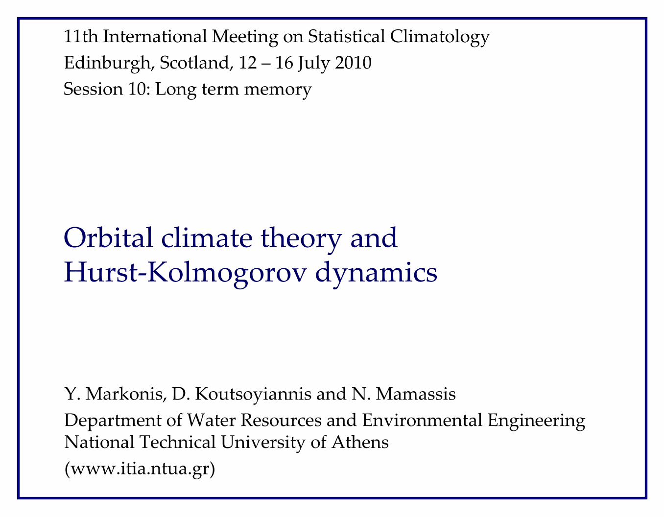
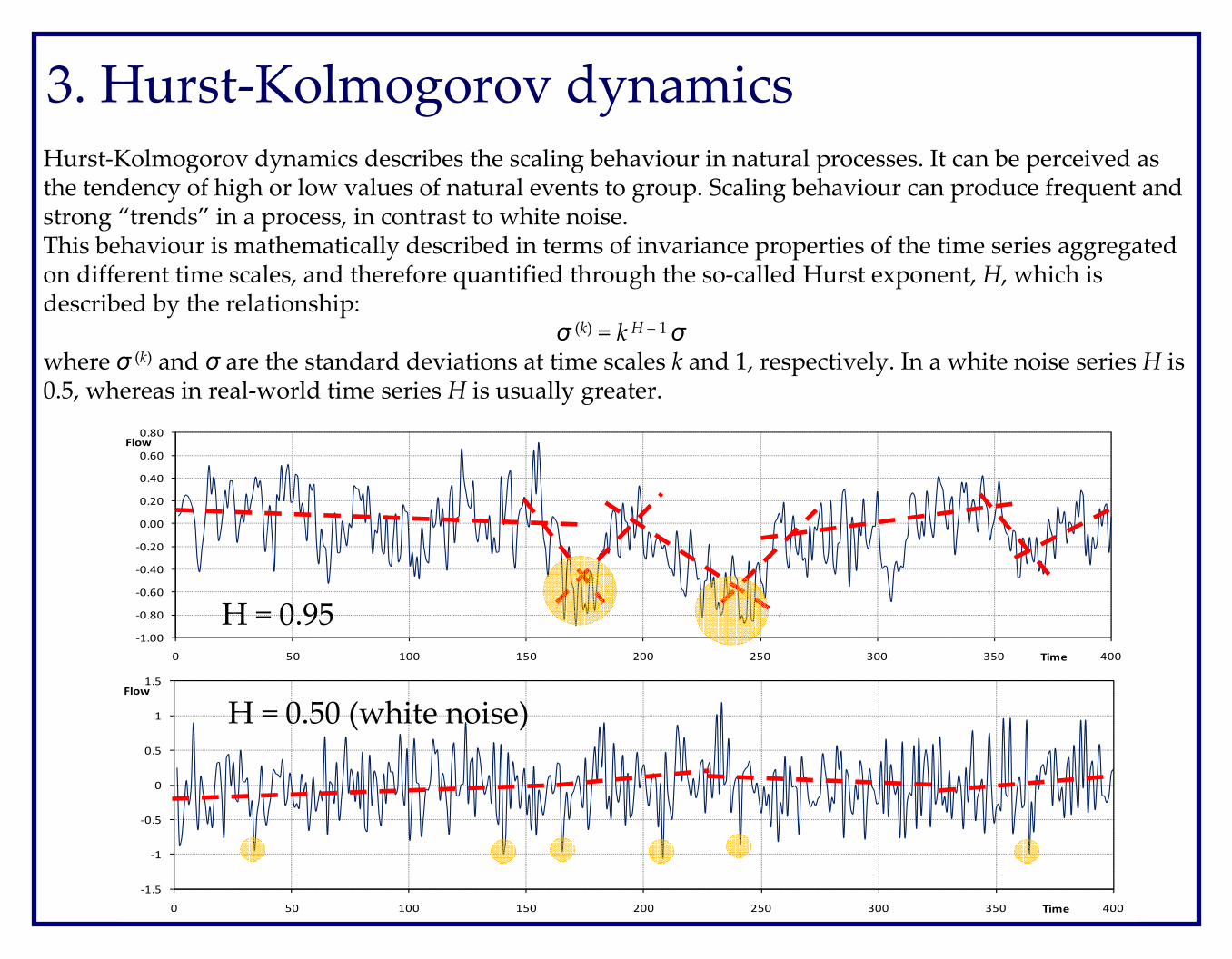
Hurst-Kolmogorov dynamics describes the scaling behaviour in natural processes. It can be perceived as the tendency of high or low values of natural events to group. Scaling behaviour can produce frequent and strong “trends” in a process, in contrast to white noise.This behaviour is mathematically described in terms of invariance properties of the time series aggregated on different time scales, and therefore quantified through the so-called Hurst exponent, H, which is described by the relationship:

σ (k) = k H – 1σ

where σ (k) and σ are the standard deviations at time scales k and 1, respectively. In a white noise series H is 0.5, whereas in real-world time series H is usually greater.

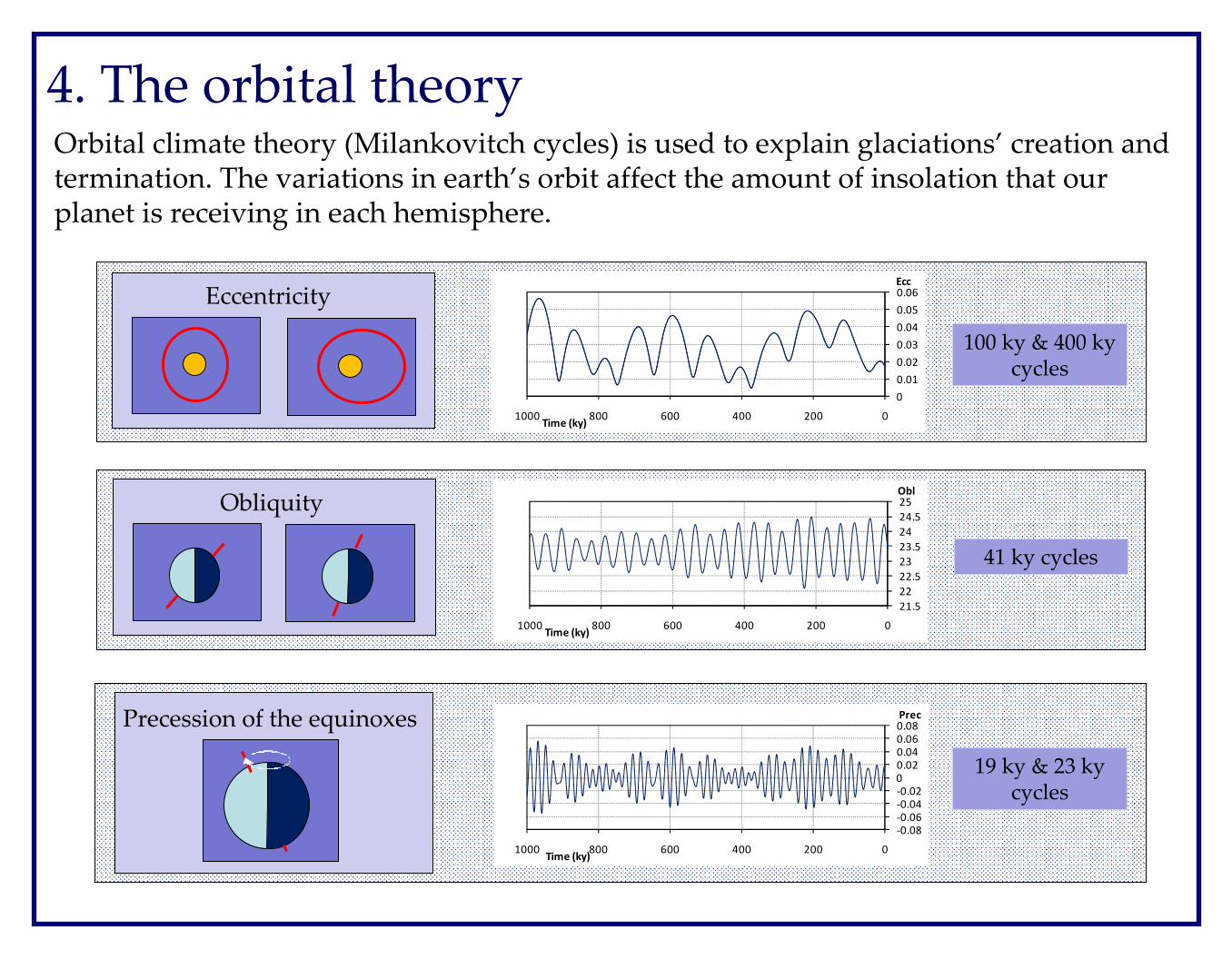
4. The orbital theoryOrbital climate theory (Milankovitch cycles) is used to explain glaciations’ creation and termination. The variations in earth’s orbit affect the amount of insolation that our planet is receiving in each hemisphere.

0

0.01

0.02

0.03

0.04

0.05

0.06

02004006008001000

Ecc

Time (ky)

Eccentricity

100 ky & 400 ky cycles

21.5

22

22.5

23

23.5

24

24.5

25

02004006008001000

Obl

Time (ky)

Obliquity

41 ky cycles

-0.08

-0.06

-0.04

-0.02

0

0.02

0.04

0.06

0.08

02004006008001000

Prec

Time (ky)

Precession of the equinoxes

19 ky & 23 ky cycles

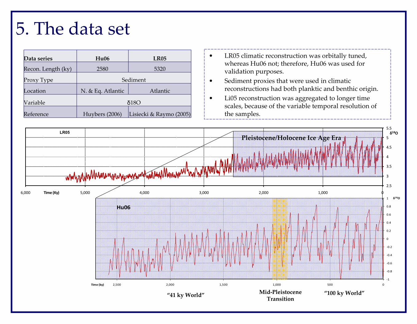
5. The data set

Data series Hu06 LR05

Recon. Length (ky) 2580 5320

Proxy Type Sediment

Location N. & Eq. Atlantic Atlantic

Variable δ18O

Reference Huybers (2006) Lisiecki & Raymo (2005)

• LR05 climatic reconstruction was orbitally tuned, whereas Hu06 not; therefore, Hu06 was used for validation purposes.

• Sediment proxies that were used in climatic reconstructions had both planktic and benthic origin.

• Li05 reconstruction was aggregated to longer time scales, because of the variable temporal resolution of the samples.

2.5

3

3.5

4

4.5

5

5.5

01,0002,0003,0004,0005,0006,000

δ18O

Time (Ky)

Li05

-1

-0.8

-0.6

-0.4

-0.2

0

0.2

0.4

0.6

0.8

1

05001,0001,5002,0002,500

δ18O

Time (ky)

Hu06

Pleistocene/Holocene Ice Age Era

Mid-Pleistocene Transition

“100 ky World”“41 ky World”

LR05

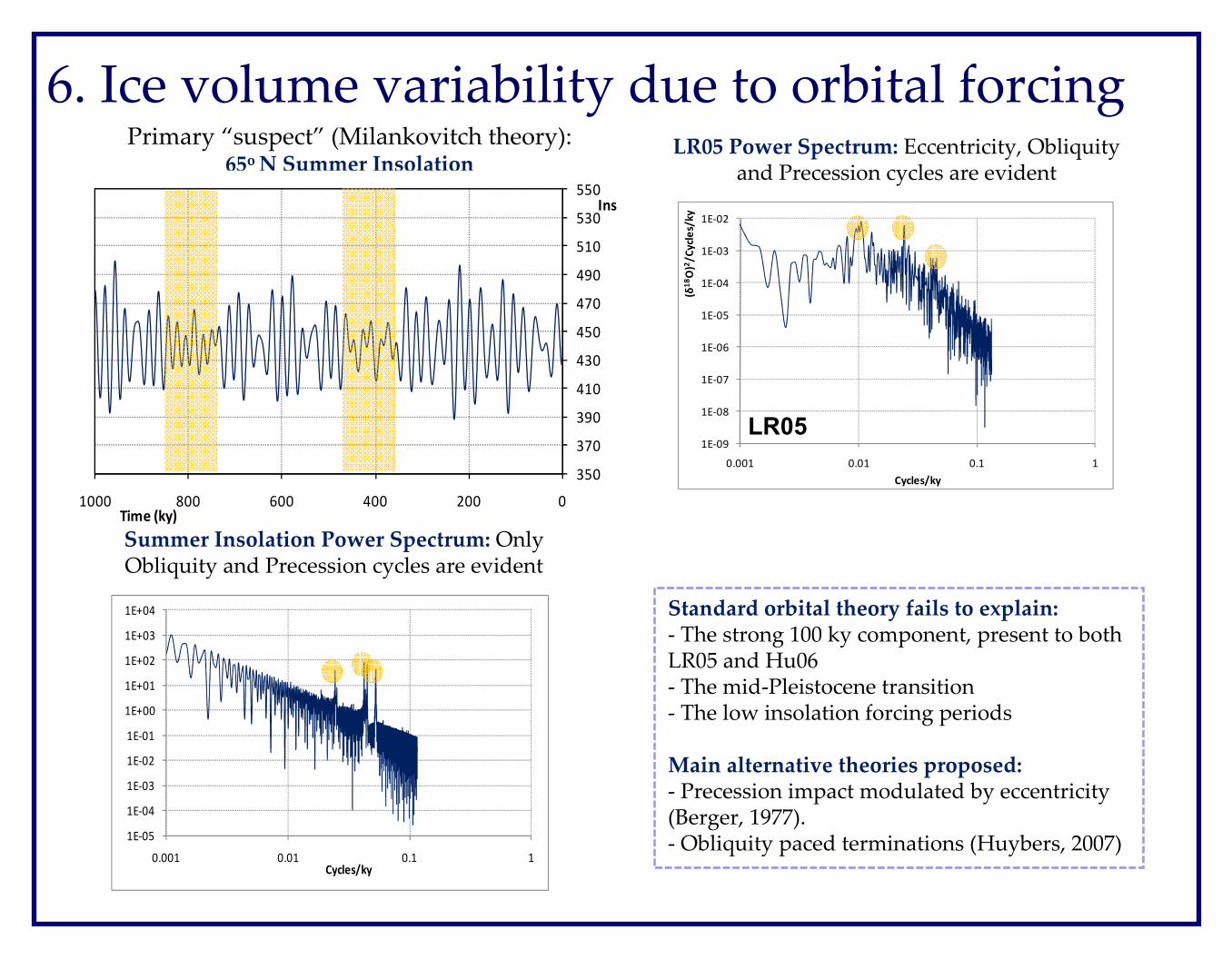
6. Ice volume variability due to orbital forcing

1E-09

1E-08

1E-07

1E-06

1E-05

1E-04

1E-03

1E-02

0.001 0.01 0.1 1

(δ1

8Ο

)2/

Cy

cle

s/k

y

Cycles/ky

LR05 Power Spectrum: Eccentricity, Obliquity and Precession cycles are evident

Primary “suspect” (Milankovitch theory):65o N Summer Insolation

350

370

390

410

430

450

470

490

510

530

550

02004006008001000

Ins

Time (ky)

Standard orbital theory fails to explain:- The strong 100 ky component, present to both LR05 and Hu06- The mid-Pleistocene transition- The low insolation forcing periods

Main alternative theories proposed:- Precession impact modulated by eccentricity (Berger, 1977).- Obliquity paced terminations (Huybers, 2007)

LR05

1E-05

1E-04

1E-03

1E-02

1E-01

1E+00

1E+01

1E+02

1E+03

1E+04

0.001 0.01 0.1 1Cycles/ky

Summer Insolation Power Spectrum: Only Obliquity and Precession cycles are evident

7. Variability due to the orbital forcing

Two harmonics were fitted for the “100ky world” and the “41ky world”, in 1/100 and 1/41 frequencies (Ecc & Obl).They explain 46% of the variability in LR05.

A harmonic fitted for the precession band contributed only 2-3% to the variability and therefore it was not used.

For Hu06, the explained variance is 36% (21% less than in LR05 -- probably, because LR05 was orbitally tuned).

The residual time series, describing the 54-64% of natural variability was examined for the presence of HK dynamics.

Fitted harmonics

Correlogram

Residuals

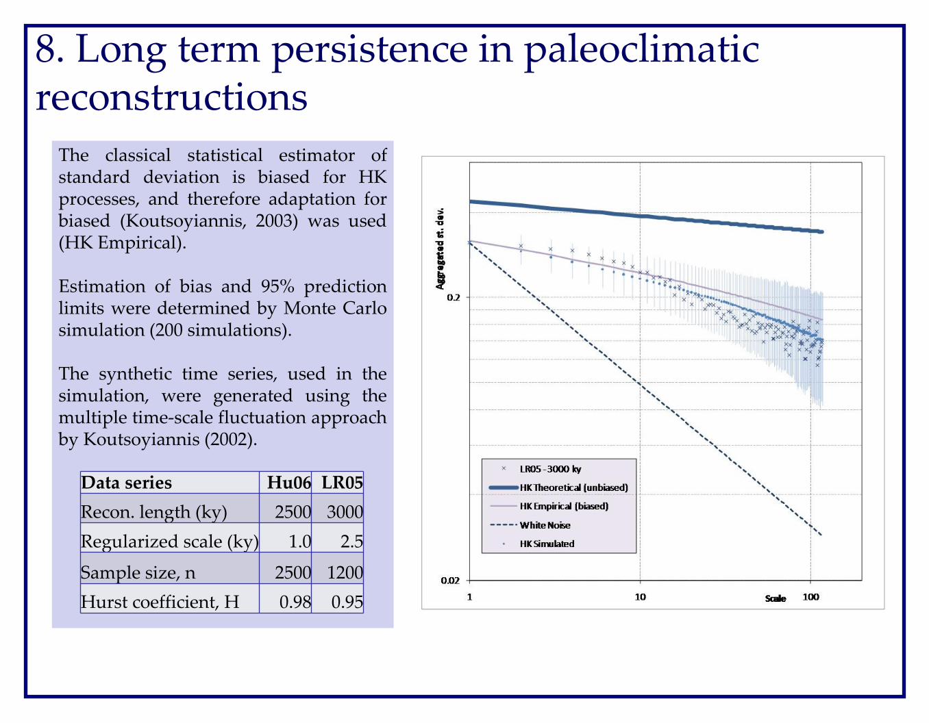
8. Long term persistence in paleoclimatic reconstructions

The classical statistical estimator of standard deviation is biased for HK processes, and therefore adaptation for biased (Koutsoyiannis, 2003) was used (HK Empirical).

Estimation of bias and 95% prediction limits were determined by Monte Carlo simulation (200 simulations).

The synthetic time series, used in the simulation, were generated using the multiple time-scale fluctuation approach by Koutsoyiannis (2002).

Data series Hu06 LR05

Recon. length (ky) 2500 3000

Regularized scale (ky) 1.0 2.5

Sample size, n 2500 1200

Hurst coefficient, H 0.98 0.95

9. A simple HK model for the ice volume variation

95% conf. interval

LR05 and the simple HK model

Glacial variability of the last 3 000 ky can be described as the sum of the eccentricity- and obliquity-fitted harmonics (deterministic part) and a HK process (stochastic part).

The simple model demonstrates similar results for Hu06.

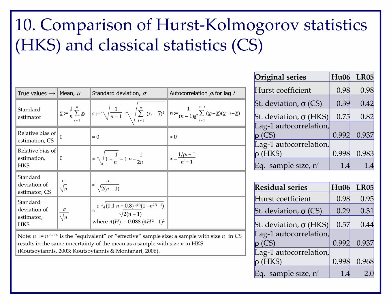
10. Comparison of Hurst-Kolmogorov statistics (HKS) and classical statistics (CS)

Original series Hu06 LR05

Hurst coefficient 0.98 0.98

St. deviation, σ (CS) 0.39 0.42

St. deviation, σ (HKS) 0.75 0.82Lag-1 autocorrelation, ρ (CS) 0.992 0.937Lag-1 autocorrelation, ρ (HKS) 0.998 0.983

Eq. sample size, n’ 1.4 1.4

True values → Mean, µ Standard deviation, σ Autocorrelation ρl for lag l

Standard

estimator x– :=

1

n ∑i = 1

n

xi s := 1

n – 1 ∑

i = 1

n

(xi – x–)2 rl := 1

(n – 1)s2 ∑i = 1

n – l

(xi – x–)(xi + l – x–)

Relative bias of

estimation, CS 0 ≈ 0 ≈ 0

Relative bias of

estimation,

HKS

0 ≈ 1 − 1

n΄ − 1 ≈ −

1

2n΄ ≈ –

1/ρl − 1

n΄− 1

Standard

deviation of

estimator, CS

σ

n ≈

σ

2(n – 1)

Standard

deviation of

estimator,

HKS

σ

n΄

≈ σ (0.1 n + 0.8)λ(H)(1 –n2H − 2)

2(n – 1)

where λ(H) := 0.088 (4H 2 – 1)2

Note: n΄ := n 2 – 2H is the “equivalent” or “effective” sample size: a sample with size n΄ in CS

results in the same uncertainty of the mean as a sample with size n in HKS

(Koutsoyiannis, 2003; Koutsoyiannis & Montanari, 2006).

Residual series Hu06 LR05

Hurst coefficient 0.98 0.95

St. deviation, σ (CS) 0.29 0.31

St. deviation, σ (HKS) 0.57 0.44Lag-1 autocorrelation, ρ (CS) 0.992 0.937Lag-1 autocorrelation, ρ (HKS) 0.998 0.968

Eq. sample size, n’ 1.4 2.0

11. Conclusions• The Hurst-Kolmogorov dynamics, also known as long-term persistence,

has been detected in paleo-climate reconstructions, dating back to 3,000 ky.

• Only a portion (36-46%) of natural variance can be described by the orbital forcing. The impact of precession of equinoxes in this portion is minimal.

• Hurst coefficient, H, demonstrates high values (approx. 0.95-0.98 for each reconstruction), which results in serious differences between the estimation of the statistical properties of the data using CS or HKS. Hurst coefficient is almost the same for the reconstruction data and the residual time series.

• The empirical data lie within the prediction limits of the HK process. Strong estimation bias is evident.

• The residual time series, describing the 54-64% of natural variance can be described as an HK processes. This is not white noise.

• The decline of the mean temperature during the last 3,000 ky could be explained as an intrinsic characteristic of HK process and not a deterministic trend.

• The comparison of statistical analysis between CS and HKS results in serious differences in the estimation of the data variability.

12. ReferencesBerger, A. (1977) Support for the astronomical theory of climatic change, Nature 268,

44–45.Hurst, H.E., (1951) Long term storage capacities of reservoirs, Trans. Am. Soc. Civil

Engrs., 116, 776–808.

Huybers P., (2007) Glacial variability over the last two million years: an extended depth-derived agemodel, continuous obliquity pacing, and the Pleistocene progression, Quat. Sci. Rev. 26, 37-55.

Kolmogorov, (1940) A. N., Wienersche Spiralen und einige andere interessante Kurven in Hilbertschen Raum, Dokl. Akad. Nauk URSS, 26, 115–118.

Koutsoyiannis D. (2002), The Hurst phenomenon and fractional Gaussian noise made easy, Hyd. Sci., 47 (4).

Koutsoyiannis D. (2003), Climate change, the Hurst phenomenon, and hydrological statistics. Hyd. Sci., 48 (1).

Koutsoyiannis D. & Montanari A. (2006), Statistical analysis of hydroclimatic time series: uncertainties and insights, Water Resour. Res. 43 (5), W05429.1-9.

Lisiecki, L. E., and Raymo, M. E. (2005), A Pliocene-Pleistocene stack of 57 globally distributed benthic d18O records, Paleoceanography, 20, PA1003.