Embed Size (px)
Citation preview

Two Dimensional Design of Axial Compressor An Enhanced Version of LUAX-C
Daniele Perrotti
Thesis for the Degree of Master of Science
Division of Thermal Power Engineering
Department of Energy Sciences
Faculty of Engineering, LTH
Lund University
P.O. Box 118
SE-221 00 Lund
Sweden


Page 1
ABSTRACT
The main scope of this thesis is to have a strong tool for a preliminar design and sizing of an
axial compressor in a bi-dimensional way, this means that all the parameters are referred to
the hub, to the midspan and to the tip of the blade.
This goal has been reached improving a pre existent MatlabTM
code based on a
monodimensional design.
The developed code, using different swirl law, allow to understand the behaviour of the flow
in both the axial and radial direction of the compressor, furthermore it plot the blade shape,
once at the midspan of each stages, so the rotor and the stator are plot togheter, once for each
blade separately, at the hub, at the mid-span and at tip, to show how the blade has to be made
to properly follow the flow.
This code has to be intended as an approach point for a more accurate design for axial
compressor, e.g. CFD, that always need a good one and bi-dimensional preliminary design to
obtain correct results; or it could be used in academic field for a better comprehension from
the student of the phenomenas that take place in this kind of machine.

Page 2
ACKNOWLEDGMENT
First of all I want to thanks Professor Magnus Genrup to give me this big opportunity to
develop a work in a really important and prospectfull field such as turbomachinery, and to
allow me to add an international experience to my studies.
Also I want to thanks the PhD students of the division of Thermal Power Engineering,
department of Energy Science at Lund University that are interested about my work, resolving
my doubts; all of this without forget Maura, whose presence permit me to feel less the lack of
my city and friend.
At last, but not the least, I want really to thanks a lot my mum and dad, without their support
and approval during the years, and their continuos encouragement, all of this could not be
possible.

Two Dimensional Design of Axial Compressor Table of Contents
Page 3
Table of Contents
CHAPTER 1 MAIN CHARACTERISTICS ............................................................................. 5
1.1 BLADE NOMENCLATURE ............................................................................................. 7
1.2 LIFT AND DRAG ............................................................................................................... 8
1.3 STALL AND SURGE ......................................................................................................... 9
1.4 TIP CLEARANCE ............................................................................................................ 10
CHAPTER 2 THEORY & MODELS ...................................................................................... 12
2.1 FUNDAMENTAL LAWS ................................................................................................. 12
2.2 DIMENSIONAL ANALYSIS ........................................................................................... 14
2.3 BI-DIMENSIONAL FLOW BEHAVIOUR ................................................................... 16
2.4 EFFICIENCY .................................................................................................................... 19
2.5 VELOCITY DIAGRAMS AND THERMODYNAMICS .............................................. 20
2.6 OFF DESIGN PERFORMANCE .................................................................................... 23
2.7 THREE DIMENSIONAL FLOW BEAHVIOUR .......................................................... 24
2.7.1 Forced vortex flow ....................................................................................................... 26
2.7.2 Free Vortex Flow (n=-1).............................................................................................. 27
2.7.3 Exponential Vortex Flow (n=0) ................................................................................... 27
2.7.4 Constant Reaction Vortex Flow (n=1) ......................................................................... 27
2.8 ACTUATOR DISK THEORY ......................................................................................... 28
2.9 COMPUTATIONAL FLUID DYNAMICS .................................................................... 29
CHAPTER 3 THEORY USED IN THE CODE ...................................................................... 33
3.1 PREVIOUS WORK .......................................................................................................... 33
3.2 OUTLET TEMPERATURE LOOP ................................................................................ 35

Two Dimensional Design of Axial Compressor Table of Contents
Page 4
3.3 SWIRL LAW ..................................................................................................................... 38
3.3.1 Forced vortex law ........................................................................................................ 38
3.3.2 General Whirl Distribution .......................................................................................... 39
Exponential Vortex Flow ..................................................................................................... 41
3.4 STAGES AND OUTLET GUIDE VANES PROPERTIES ........................................... 43
3.4.1 Rotor inlet .................................................................................................................... 43
3.4.2 Stator inlet .................................................................................................................... 44
3.4.3 Stator outlet .................................................................................................................. 46
3.4.4 Outlet Guide Vanes (OGV) .......................................................................................... 47
3.5 BLADE ANGLES AND DIFFUSION FACTOR ........................................................... 48
3.5.1 Rotor............................................................................................................................. 48
3.5.2 Stator blade angles....................................................................................................... 50
3.6 BLADE SHAPE ................................................................................................................. 51
CHAPTER 4 APPLICATION .................................................................................................. 54
CHAPTER 5 USER’S GUIDE .................................................................................................. 58
Bibliography ..................................................................................................................................... 60
A, Table of figures ………………………………………………………………………....................59
B, Matlab Code ………………………………………………………………………………………...60
B1, Forced Vortex Law ……………………………………………………………………………….60
B2,General Whirl Distribution ………………………………………………………………………67
B3, Blade Shape Plot ………………………………………………………………………………….83
B4, Blade Shape Hub To tip Plot …………………………………………………………………....90
B5, Main Calculation ………………………………………………………………………………..114
C, Results ……………………………………………………………………………………………...135

Two Dimensional Design of Axial Compressor Main Characteristics
Page 5
CHAPTER 1 MAIN CHARACTERISTICS
In everyday life compressors are becoming more and more fundamental, from the production
of energy to the transport field, they assumed a strong role for enhance the human condition.
Their operating principle were established more than sixty years ago, and during the last
decades all the efforts have been concentrated on how to improve and develop better
machine, and on the study of the behaviour of the elaborated flow.
Figure 1-1 Pressure ratio increase along the years
Dynamic compressors are divided in two big family, axial compressor and radial compressor,
the choice between them it’s the consequence of the valuation of multiple parameters, and it
will be work of the designer to find the correct one.
Figure 1-2 Axial and Radial compressor
Two Dimensional Design of Axial Compressor Main Characteristics
Page 6
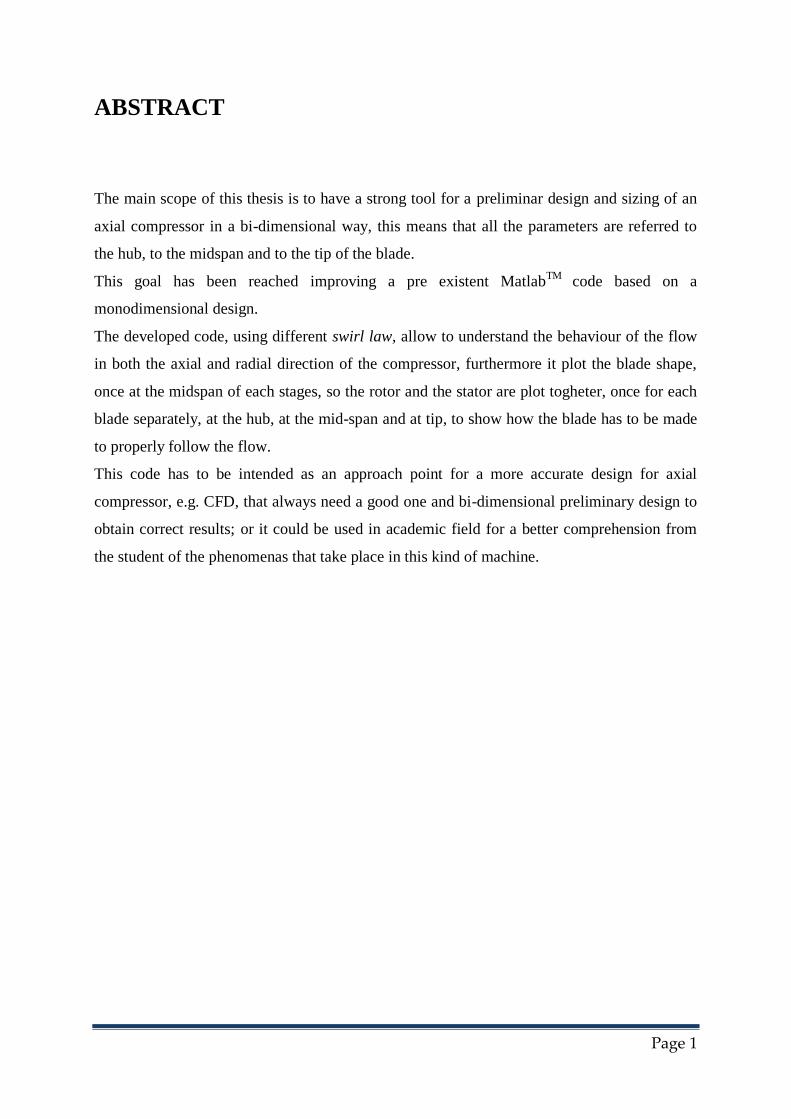
Axial compressor can elaborate a higher flow than the radial, which has a higher pressure
ratio per stage, this means that for the same flow rate the firsts will have a smaller diameter,
but it will need more stages to reaches the same pressure ratio.
Another aspect to consider is the efficiency, which reaches better values in the axial one,
because the flow withstand less changes of direction along the stages, with minor perturbation
through each blade row.
For the same mass flow and pressure ratio radial compressor are cheaper than the other,
furthermore they are more resistant in case of damage caused by external object.
In figure 1.2 is it possible to see the behaviour of both compressors in relation to velocity and
pressure ratio, is it clear that radial compressors have more margin to the surge, and axial
compressor should be used only at high speed.
Figure 1-3 Comparison of axial centrifugal characteristic curves (Dresser-Rand)
The main character of this thesis is the axial compressor, which is become the main choose
for the most of the application from gas turbine for electric energy production, because of the
growth of turbogas plant, to engine for aircraft.
The increase of efficiency in gas turbine has been obtained from the increase in pressure ratio
in the compressor and the increase in firing temperature in the combustion chamber; in the
axial compressor the total pressure ratio is due to the sum of the increase obtained in each
stage, which is limited to avoid high diffusion.

Two Dimensional Design of Axial Compressor Main Characteristics
Page 7
1.1 BLADE NOMENCLATURE
Generally an axial compressor is compose by a variable number of stages where each follow
one other, a single stage is made up by a rotor and a stator; both of them present blades
disposed in a row, called cascade.
A blade has a curved shape, convex on one side, called suction side, and concave on the other,
called pressure side, the symmetric line of the blade is the camber line, whereas the line
which connect directly the leading and trailing edge is the chordline, the distance between
these two line is the camber of the blade.
The turning angle of the camberline is called camber angle, ϑ, and the angle between the
chordline and the axial direction is the stagger angle, γ ( Figure 1-4).
thickness of the blade, t
flow angle, α
blade angle, α’
staggered spacing, s
incidence, i=α1- α’1
deviation, δ= α2- α’2
camber angle, ϑ= α’1-α’2
Figure 1-4 Blade nomenclature
Only at ideal condition the incidence angle will be equal to zero, but for common operational
condition it often has different values that could be negative or positive.
The deviation is always greater than zero, because the flow is not able to follow precisely the
shape of the blade due to its inertia.
The difference between the inlet flow angle and the outlet one, is called deflection, ε, this
changing in the flow direction is the real responsible of the change in momentum.
The thickness distribution depends from the blade type, a common kind of profile is the
NACA-65 series cascade profile, in this thesis a double circular arc has been adopted for the
airfoil.

Two Dimensional Design of Axial Compressor Main Characteristics
Page 8
1.2 LIFT AND DRAG
The reaction forces which the blade exert on the flow are called drag and lift, the first act in
the same direction of the stream, the second is perpendicular, it arise because the speed of the
flow on the suction surface in greater than the flow on the pressure surface, thus, by the
Bernoulli equation, the pressure on the under surface is bigger than the one of the upper side
of the blade (Figure 1-5).
Figure 1-5 Drag and Lift forces
In order to calculate these two forces, the following relations can be used:
(1.1)
(1.2)
Where A is the obstruction of the blade in the flow direction, ρ is the density, c is the velocity
of the flow, and CD and CL are respectively the coefficient of drag and the coefficient of lift,
calculated from experimental dates.
Those two coefficients are strongly influenced by the attack angle, α, in particular, the lift
coefficient after a certain values of the incidence goes to zero, this means that stall happen on
the blade and it stop to interact with the fluid (Figure 1-6). In a compressor, this entails a drop
in the pressure increase and a reduction in all its performance.

Two Dimensional Design of Axial Compressor Main Characteristics
Page 9
Figure 1-6 Lift and Drag coefficient
1.3 STALL AND SURGE
A compressor has more criticality than a turbine, this, basically, because the flow is forced to
move from a zone with low pressure in another at high pressure, that is an unnatural
behaviour.
At low blade speed, rotating stall may occur, this phenomena belong to the progressive stall
family; the blade stall each separately from the others, and this stall patch moves in the
opposite direction of the rotation of the shaft. This happen because the patch reduces the
available section for the flow to pass between two adjacent blades, so it is deflected on both
sides of the cascade (Figure 1-7).
This implies that the incidence of the flow on the left side is increased and the incidence of
the flow on the right side is reduced; the frequency with which the stall interests each blade
can be near to the natural frequency of blade vibration causing its failure.
Progressive stall is typical of the transitory, but it can be controlled by bleeding the flow from
the intermediate stages or using blade with variable geometry, inlet guide vanes (IGV), or
both of them.
The most dangerous and disruptive phenomena in compressor is the surge, it is the lower limit
of stable operation, it occurs when the slope of the pressure ratio versus mass flow curve
reaches zero.

Two Dimensional Design of Axial Compressor Main Characteristics
Page 10
When the inlet flow is reduced, the output pressure reaches its maximum, if the flow is
reduced more, the pressure developed by the compressor became lower than the pressure in
the discharge line, and the flow start to move in the opposite way.
Figure 1-7 Rotating stall
The pressure at the outlet is reduced by the reverse of the flow, thus normal compression start
again; since no change in the compressor operation is done, the entire cycle is repeated. The
frequency of this phenomenon can be the same of the natural frequency of the components of
the compressor, causing serious damage, especially to blades and seals.
Surge is linked with increase in noise level and vibration, axial shaft position change, pressure
fluctuation, discharge temperature excursions.
Stall and surge should not be confused even if the past happened, surge must be total avoid,
but a multi-stage compressor may operate stably even if one or more stages stalled, treating
the compressor casing may avoid this last phenomenon.
Another operating limit of the compressor is choking, it happen when the flow in the blades
throat reaches a Mach number of 1.0, in this case the slope of pressure ratio versus mass flow
curve coming on infinite, thus the elaborated mass flow cannot be increased more.
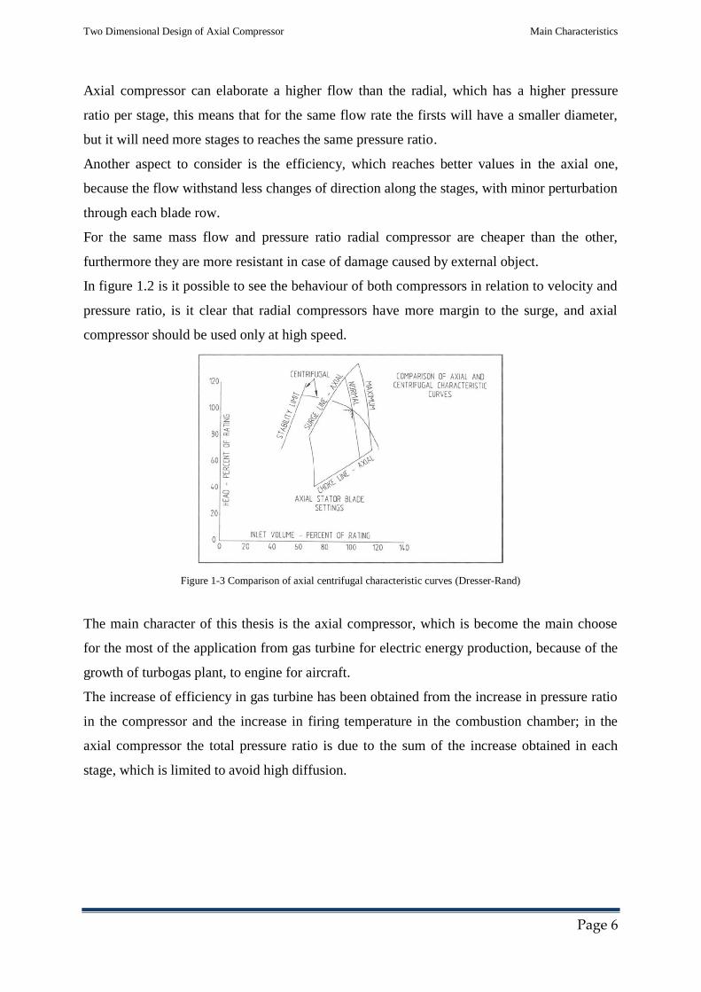
1.4 TIP CLEARANCE
To avoid rubbing between the rotor and its surrounding casing during rotation, there must be a
small clearance, this, linked with the pressure difference across the blade, create a tip
clearance flow through this tiny space, forming a tip leakage vortex (Figure 1-8).
Two Dimensional Design of Axial Compressor Main Characteristics
Page 11
Figure 1-8 Tip clearance flow (Berdanier)
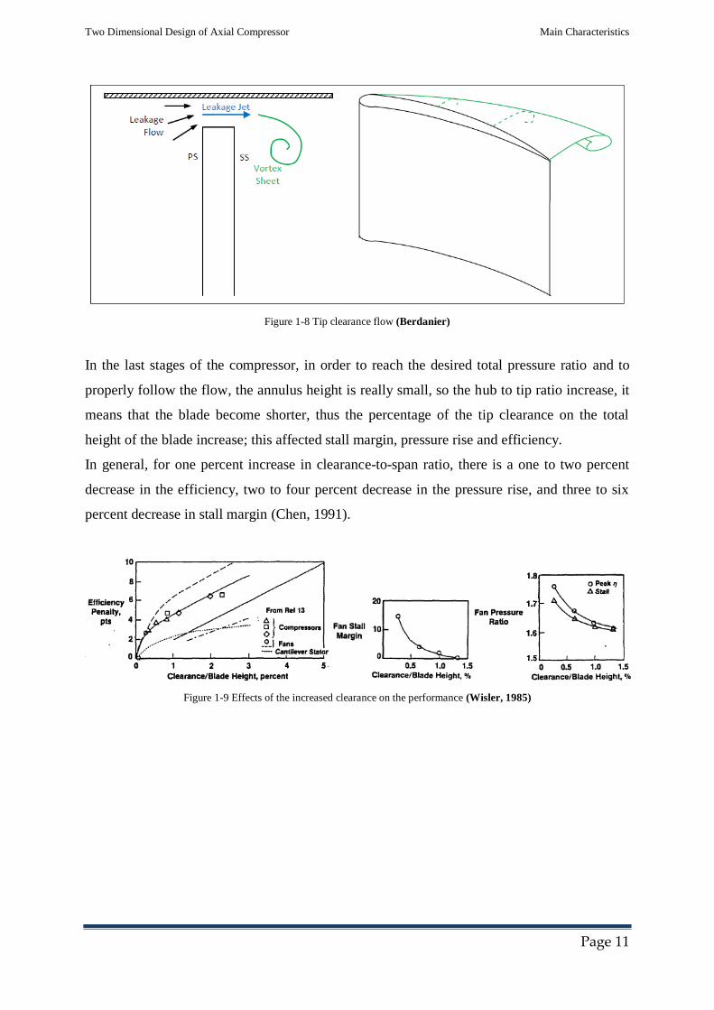
In the last stages of the compressor, in order to reach the desired total pressure ratio and to
properly follow the flow, the annulus height is really small, so the hub to tip ratio increase, it
means that the blade become shorter, thus the percentage of the tip clearance on the total
height of the blade increase; this affected stall margin, pressure rise and efficiency.
In general, for one percent increase in clearance-to-span ratio, there is a one to two percent
decrease in the efficiency, two to four percent decrease in the pressure rise, and three to six
percent decrease in stall margin (Chen, 1991).
Figure 1-9 Effects of the increased clearance on the performance (Wisler, 1985)

Two Dimensional Design of Axial Compressor Theory & Models
Page 12
CHAPTER 2 THEORY & MODELS
In this chapter it will be presented a review of the modelling concerned turbomachinery,
starting from Euler work equation until CFD model, passing throughout bi-dimensional and
three-dimensional flow.
2.1 FUNDAMENTAL LAWS
It is possible to write the elementary rate of mass flow like
(2.1)
where d is the element of area perpendicular to the flow direction, c is the stream velocity
and the fluid’s density.
In one dimensional steady flow, where we can suppose constant velocity and density, defining
two consecutive station, 1 and 2, without accumulation of fluid in the control volume, it is
possible to write the equation of continuity:
(2.2)
The fundamental law used in turbomachinery field is the steady flow energy equation:
[( )
(
) ( )]
(2.3)
but, some observation can be do, first of all flow process in this field are adiabatic, so it is
possible to consider equal to zero, than the quote different ( ) is very small and can
be ignored, thus, considering that compressors absorbed energy we can write:
( ) (2.4)

Two Dimensional Design of Axial Compressor Theory & Models
Page 13
h0 is called stagnation enthalpy and is the combination of enthalpy and kinetic energy:
(2.5)
For a compressor the work done by the rotor is
( ) (2.6)
where is the sum of the moments of the external forces acting on fluid, U is the blade speed
and the tangential velocity. So the specific work is
(2.7)
also called Euler work equation.
Combining equation (2.4) and (2.7) it is possible to obtain the relation between the two
stations, which in our case are the inlet and the outlet of the rotor and the stator:
(2.8)
those two terms are known as rothalpy I, which is constant along a single streamline through
the turbomachine; it is also possible to refer it at the relative tangential velocity becoming
( ) ( )
(2.9)
having define the relative stagnation enthalpy as
(2.10)

Two Dimensional Design of Axial Compressor Theory & Models
Page 14
In the turbomachinery field is not possible to consider the fluid incompressible anymore, due
to the Mach number that is bigger than 0.3; using the local value of this parameter we can
relate stagnation and static temperature, pressure and density:
(2.11)
(
)
( )⁄
(2.12)
(
)
( )⁄
(2.13)
Combining these three equations and the continuity one, non-dimensional mass flow rate is
obtained:
√
√ (
)
(
)
(2.14)
also known as flow capacity.
2.2 DIMENSIONAL ANALYSIS
With this procedure is possible to reproduce physical situation with few dimensionless group,
applying it at turbomachines lead first to predict the performance of a prototype from test
conducted on a scale model, this is called similitude, and second, to determine the most
appropriate kind of machine, for a specified range of speed, flow rate and head, based on the
maximum efficiency.
For compressible fluid the performance parameters, which are isentropic stagnation enthalpy
change ∆h0s, efficiency η and power P can be expressed as function of:
( ) (2.15)

Two Dimensional Design of Axial Compressor Theory & Models
Page 15
where µ is the viscosity of the fluid, N is the speed of rotation, D the impeller diameter and
a01 is the stagnation speed of sound at the inlet; selecting N, D and ρ01 as common factors it is
possible to write the last relationship with five dimensionless groups:
(
) (2.16)
With some passage and considering machine that operate with a single gas and at high
Reynolds number it is possible to write it like:
(
√
√
) (2.17)
it is clear that to fix the operating point of a compressible flow machine, only two variables
are required.
The performance parameters are not independent one each others, but with the equation of the
isentropic efficiency, we can link them together:
[( ⁄ ) ( )⁄ ]
⁄ (2.18)
Two of the most important parameters of the compressible flow machine, are flow coefficient
and stage loading, the first is
(2.19)
where cm is the average meridional velocity, and the second is
(2.20)
both of them can be related to the non-dimensional mass flow √
and non-dimensional
blade speed
√ .

Two Dimensional Design of Axial Compressor Theory & Models
Page 16
Equation (2.17) can be graphically represented in the performance map of high speed
compressor (Figure 2-1), surge line is the upper operative limit of any single speed line, above
this line aerodynamic instability and stall will occur; the other limit, the lower, is the choke
line, this phenomena happen when the flow reaches the velocity of sound, at this point, the
mass flow cannot be increase anymore.
Figure 2-1 Characteristic curves of the compressor (Johnson & Bullock, 1965)
For a correct choice of turbomachinery for a given duty, designers use two non-dimensional
parameters, specific diameter Ds, and specific speed Ns; for a compressible fluid machine, find
this last parameter allow to determine, for a particular requirement, the better choice between
radial and axial flow machine.
⁄
( ) ⁄ (
) ⁄
( ) ⁄ (2.21)
2.3 BI-DIMENSIONAL FLOW BEHAVIOUR
It is not possible to consider a monodimensional trend of the stream flow in an axial
turbomachinery, because the fluid which passes throughout any blade row will have three
components: axial, tangential and radial.
For hub-to-tip ratio more than 4/5 it is possible to assume the radial component equals to zero,
but under this limit is not possible to consider anymore streamlines lying on the same radius
for the entire machine (Figure 2-2).

Two Dimensional Design of Axial Compressor Theory & Models
Page 17
Figure 2-2 Radial shift of streamlines through a blade row (Johnson & Bullock, 1965)
Before introduce radial equilibrium theory which rules the three dimensional behaviour we
analyse the bidimensional one.
The flow will never follow entirely the blade angle because of its inertia, thus it will leave the
trailing edge with a different angle respect to blade exit angle, this means that the boundary
layers on the suction and pressure surface growth along the blade and with them the cascade
losses (Figure 2-3).
Another cause of the growth of the boundary layers, is the rapid increase in pressure that
produce a contraction on the flow, to consider this, a useful parameter it is been introduced,
the axial velocity density ratio:
(2.22)
where H is the projected frontal area of the control volume.
Figure 2-3 Boundary layer (Johnson & Bullock, 1965)

Two Dimensional Design of Axial Compressor Theory & Models
Page 18
Furthermore the increase of the diffusion, which is large in a compressor, tends to produce
thick boundary layers and flow separation, specially on the suction surface of the blade, this
lead to an alteration of the free stream velocity distribution (Figure 2-4) and loss in total
pressure.
To consider this phenomena Lieblein, Schwenk and Broderick developed a parameter, called
diffusion factor, which is really usefull during the design phase.
(
) (
)
(2.23)
when this factor exceeds 0.6 the flow start to separate, so is common to operate with a value
of 0.45 in order to prevent losses.
s/c is the pitch chord ratio, also know as the inverse of solidity σ, more used in the U.S., a low
values means that across the blade passage is required a lower pressure increase to turn the
flow, and the diffusion is restrain, furthermore, with a small value a blade row will have more
blade than another with a higher values and the loading will be share better between the
blades, but a high values of the chord implies more loss due to the higher wetted area and a
longer and more expensive machine; so it is very important to choose an accurate values for
the pitch chord ration, because also the shape of the blade, and the interaction between them
depends from it, a typicall value for pitch chord ratio is between 0.8 and 1.2.
Figure 2-4 Velocity distribution and flow separation (Johnson & Bullock, 1965)
To avoid high diffusion, de Haller proposed to control the overall deceleration ratio, both in
the rotor and in the stator; the minimum value fixed by him is 0.72 so:
(2.24)

Two Dimensional Design of Axial Compressor Theory & Models
Page 19
2.4 EFFICIENCY
In turbomachinery field, the efficiency can be expressed in several ways, the most useful are
the isentropic and the polytropic ones.
The first relates the ideal work per unit flow rate per second to the actual work per unit flow
rate per second:
(2.25)
The real work, represented from the denominator will always be bigger than the ideal work
which the compressor needed, due to the energy losses for friction.
Because of the constant pressure lines on an (h,s) diagram will diverge, at the same entropy,
the slope of the line representing the higher pressure will be greater; this means that the work
supplied in a series of isentropic process, that can be compared to the single stages in an axial
compressor, will be more than the isentropic work in the full compression process.
Therefore it is possible to define the efficiency of a compression through a small increment of
pressure dp:
(2.26)
And after several algebraic passages and using Gibbs equation, it is possible to write it like:
(
)
∫ ( )
(2.27)
If this efficiency is constant across the compressor, then ηisen will be lesser, anyway a
relationship exist between those two efficiencies (Figure 2-5):
( ( ) )
(
)
(2.28)

Two Dimensional Design of Axial Compressor Theory & Models
Page 20
Figure 2-5 Relation between isentropic efficiency , polytropic efficiency and pressure ratio
2.5 VELOCITY DIAGRAMS AND THERMODYNAMICS
For axial machine the relative stagnation enthalpy is constant across the rotor, from equation
(2.10) we can write:
(2.29)
for the stator is the same for the stagnation enthalpy:
(2.30)
Figure 2-6 Mollier Diagram

Two Dimensional Design of Axial Compressor Theory & Models
Page 21
For each stage of the compressor, a first approach can be done considering that the direction
of the fluid and its absolute velocities are the same at the inlet and the outlet, whereas the
relative velocity in the rotor and the absolute one in the stator decrease (Figure 2-7).
In the rotor the flow is turned from β1 to β2, after that the stator blades deflected it from α2 to
α3 which is assumed as equal as α1.
Figure 2-7 Velocity diagram in a compressor stage
Here is possible to define all the component of a two dimensional stream flow:
c1 absolute velocity at the rotor’s inlet
w1 relative velocity at the rotor’s inlet
cx1 axial velocity at the rotor’s inlet
cϑ1 absolute tangential velocity at the rotor’s inlet
wϑ1 relative tangential velocity at the rotor’s inlet
U blade speed
c2 absolute velocity at the rotor’s outlet
w2 relative velocity at the rotor’s outlet
cx2 axial velocity at the rotor’s outlet
cϑ2 absolute tangential velocity at the rotor’s outlet
wϑ2 relative tangential velocity at the rotor’s outlet
c3 absolute velocity at the stator’s outlet
cx3 axial velocity at the rotor’s inlet
since we are in a condition of repetitive stage the absolute velocity at the outlet of the stator
will be the same at the inlet of the following rotor.

Two Dimensional Design of Axial Compressor Theory & Models
Page 22
The velocity diagrams are strictly connected to the choice of parameters like reaction, flow
coefficient and stage loading, the last one has to be limited in order to prevent flow separation
from the blade.
( ) (2.31)
but it can also be written like
( ) ( ) (2.32)
where (tan -tan ) is the flow turning in the rotor, this means that if the flow coefficient
increases, for a fixed stage loading, the required value of that term will be lesser.
As regard the reaction, the connection with the velocity triangles can be written as
( )
( ) (2.33)
or
( )
(2.34)
Combining equation (2.31) with (2.33) we obtain:
( ) (2.35)
which gives the flow angle for the stator:
⁄
⁄
(2.36)
and for the rotor:

Two Dimensional Design of Axial Compressor Theory & Models
Page 23
⁄
⁄
(2.37)
From this it is clear how reaction can influence the fluid outlet angles from each blade row
(Figure 2-8):
If R= 0.5 from the equation (2.33) α1=β2 and the diagram is symmetrical
If R>0.5 α1<β2 and the diagram is inclined to the right
If R<0.5 α1>β2 and the diagram is inclined to the left
Figure 2-8 Influence of Reaction on Velocity diagram (Dixon & Hall, 2010)
2.6 OFF DESIGN PERFORMANCE
Considering equation (2.31), Horlock suggest that the fluid outlet angles does not change for a
variation of the inlet angle up to the stall point, so it is possible to write:
(2.38)
the value of t is given by the values chosen for ψ and Φ.
Test’s results from Howell demonstrate that α1 and β2 are not constant far from the design
point, in figure (Figure 2-9) there is the comparison between the assumption of Horlock and
the results obtained by Howell.

Two Dimensional Design of Axial Compressor Theory & Models
Page 24
Figure 2-9 Comparison of analysis with result from measure
2.7 THREE DIMENSIONAL FLOW BEAHVIOUR
In order to make an accurate analysis of the flow stream it is essential to introduce the radial
component of the velocity, this exist because there is a temporary imbalance between the
radial pressure and the centrifugal forces that acted on the flow (Figure 2-10).
The radial equilibrium theory, which is used for three-dimensional design, consider the flow
outside a blade row in a radial equilibrium, it means that in a generic station sufficiently far
from the blade, the stream flow can be considered axisymmetric so all the parameters are the
same for each cascade of the same row.
In ϑ direction, forces of inertia and force of pressure does not exist, thus, we can write the
equilibrium only for the radial direction:
( )( ) (
)
(2.39)
Figure 2-10 Forces acting on a fluid element

Two Dimensional Design of Axial Compressor Theory & Models
Page 25
The RHS of the equation (2.38) is the force of inertia which is centrifugal, the LHS is the
pressure component, ignoring second order’s terms or smaller and writing dm=ρrdrdϑ we
obtain
(2.40)
this is the conservation of momentum in the radial direction.
Knowing and ρ it is possible to obtain the radial pressure variation along the blade:
∫
(2.41)
The general form of the radial equilibrium equation for compressible flow may be obtained
using also stagnation enthalpy and entropy:
( ) (2.42)
If the terms in the LHS are constant with radius, we have:
( ) (2.43)
From this equation, choosing a distribution for the tangential velocity it is possible to obtain
the axial velocity one, this is very useful for the indirect problem; some of the distributions
used for are:
Forced vortex flow
Free vortex flow
Exponential vortex flow
Constant reaction vortex flow

Two Dimensional Design of Axial Compressor Theory & Models
Page 26
2.7.1 Forced vortex flow
In this law cϑ varies directly with the radius:
(2.44)
It means that the bending moment grew with the radius, so the blade will be high stressed;
about the axial velocity at the inlet, from equation (2.43) we obtain
(2.45)
The work distribution will not be uniform along the blade:
( ) ( ) (2.46)
Combining this with equation (2.41) lead to find the outlet axial velocity:
( ) (2.47)
It is possible to find the constant from the continuity of mass flow:
∫
∫
(2.48)
The forced vortex law is much utilized in practise because the difference between inlet and
outlet axial velocity for each stage is very low, so the diffusion is restrain and the margin to
the stall is remarkable.
The other three laws are obtained from the general whirl distribution, simply choosing
different n values:
(2.49)
(2.50)

Two Dimensional Design of Axial Compressor Theory & Models
Page 27
where a and b are constants, with this choice the work will always be constant with the radius.
2.7.2 Free Vortex Flow (n=-1)
In this case decrease with the radius:
(2.51)
and the angular momentum (cϑr) is constant, using equation (2.43) it is clear that cx will be
constant everywhere.
The work distribution is independent from the radius and the tangential forces over the blade
decreases with it, but this kind of law will require a highly twisted rotor blade even if
conservative dimensionless performance parameters are used (Aungier, 2003).
Another disadvantage is the marked degree of reaction with radius, which become negative
near the hub; this means that because of the lower blade speed at the root section, more fluid
deflection is required for the same work input, this entail a high diffusion that can lead to stall
(Saravanamuttoo, Rogers, Cohen, & Straznicky, 2009).
2.7.3 Exponential Vortex Flow (n=0)
The main advantage to use this design law is the chance to have constant camber stator blade,
also with constant stagger angle, with an accurate choice of φ, ψ, at the references radius, this
is a good way to reduce manufacturing cost; furthermore, with this design it is possible to
obtain the higher hub reaction for any choice of the reference one (Aungier, 2003), and a
reduced maximum Mach number for the rotor (Horlock, 1958).
2.7.4 Constant Reaction Vortex Flow (n=1)
This is the type of project law that more than the others let us to get close to the constant
reaction, by the way this result will never be achieved, because Φ is not constant across the
rotor, and the reaction at the reference radius should be equals to 1.
The main problem of this design is that the axial velocity at the rotor outlet could reach zero
near the tip radius, so this zone is a reverse flow zone which is unacceptable, to avoid this Φ
at the reference radius must be increased.
Two Dimensional Design of Axial Compressor Theory & Models
Page 28
This kind of law offers a good margin from stall because the velocity ratios across the blade
rows are limited.
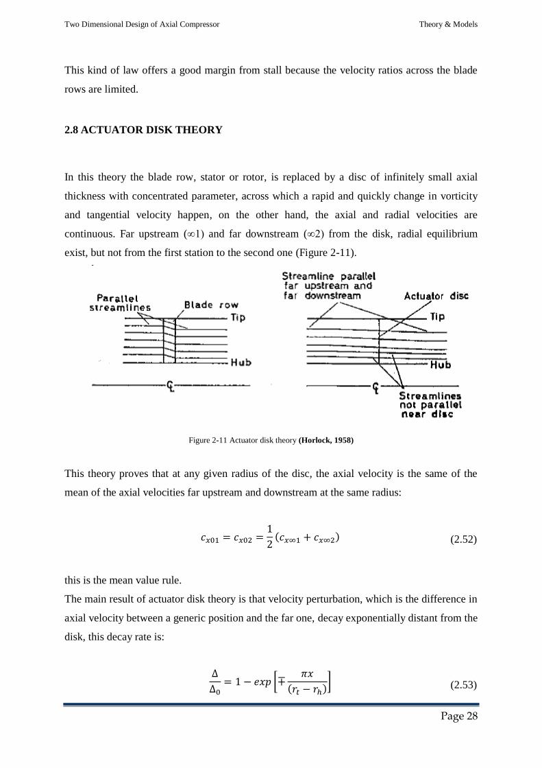
2.8 ACTUATOR DISK THEORY
In this theory the blade row, stator or rotor, is replaced by a disc of infinitely small axial
thickness with concentrated parameter, across which a rapid and quickly change in vorticity
and tangential velocity happen, on the other hand, the axial and radial velocities are
continuous. Far upstream (∞1) and far downstream (∞2) from the disk, radial equilibrium
exist, but not from the first station to the second one (Figure 2-11).
Figure 2-11 Actuator disk theory (Horlock, 1958)
This theory proves that at any given radius of the disc, the axial velocity is the same of the
mean of the axial velocities far upstream and downstream at the same radius:
( ) (2.52)
this is the mean value rule.
The main result of actuator disk theory is that velocity perturbation, which is the difference in
axial velocity between a generic position and the far one, decay exponentially distant from the
disk, this decay rate is:
[
( )] (2.53)

Two Dimensional Design of Axial Compressor Theory & Models
Page 29
where ∆ is the perturbation in a generic point and ∆0 the one at the disc (Figure 2-12).
Figure 2-12 Velocity perturbation in the Actuator disk (Dixon & Hall, 2010)
Combining equation (2.51) and (2.52) is it possible to find the axial velocity value for a
generic position:
( ) [
( )] (2.54)
( ) [
( )] (2.55)
In axial turbomachinery field, where the space between consecutive blade rows is very small
implying mutual flow interaction and strong interference effects, this theory is really useful,
because this interaction may be calculated simply extending the result obtained from the
theory for the isolated disk.
2.9 COMPUTATIONAL FLUID DYNAMICS
Flow behaviour in the compressor is highly three-dimensional, due to low aspect ratio, corner
separation, growth of boundary layers, endwall flow, tip clearance flow, hub corner vortex
(Figure 2-13), so using actuator disk theory to the design of turbomachinery implies limitation
in the final results.

Two Dimensional Design of Axial Compressor Theory & Models
Page 30
During the past two decades the use of computational fluid dynamics (CFD) in the design of
axial compressor has growth, thanks also to the increase of power of the calculators in the last
years.
The main purpose of CFD is to solve the systems of equation that describe fluid flow
behaviour: conservation of mass, Newton’s second law and conservation of energy, for a
given set of boundary condition. This system of equation is formed by unsteady Navier-
Stokes equations, which are differential equations, and they must be converted in a system of
algebraic equation to represent the interdependency of the flow at some point to the nearer
ones. The main purpose of CFD is to solve the systems of equation that describe fluid flow
behaviour: conservation of mass, Newton’s second law and conservation of energy, for a
given set of boundary condition. This system of equation is formed by unsteady Navier-
Stokes equations, which are differential equations, and they must be converted in a system of
algebraic equation to represent the interdependency of the flow at some point to the nearer
ones.
Figure 2-13 3D flow structure (Xianjun, Zhibo, & Baojie, 2012)
The points in which the values and the property of the fluid are evaluated, are set and
connected together with a numerical grid, also called mesh (Figure 2-14); the accuracy of the
numerical approximation strictly depend from the size of the grid, more is dens, better is the
approximation of the numerical scheme, however this will increase the computational cost,
also in terms of time for the iterations.

Two Dimensional Design of Axial Compressor Theory & Models
Page 31
Figure 2-14 Example of mash
In the field of turbomachinery, where the flow is very unsteady, this discretisation besides the
space domain must be done also for the time one, to achieve this, the solution procedure is
repeated several times at discrete temporal intervals.
The most important step in CFD is defining the boundary condition, it will have a great
influence on the quality of solution; at the inlet, flow conditions, total pressure, total
temperature and velocity components must be specified .
For the exit boundary conditions the best result are obtained using the static pressure outlet to
achieve the required mass flow.
Another type of boundary conditions are defined for the blade surface also considering hub
with a rotating wall boundary, and shroud; to simulate repeating blade rows, periodic
boundaries should be used for the passage sides of the grid (Figure 2-15).
After that the software has solved the governing equations for the discretised domain, the last
step of the process is the analysis of the converged solution.
CFD has to be considered complementary to experimental approach and theoretical one, and
not a substitute of them, one and bi-dimensional preliminary design are still fundamentals to
obtain a good result from CFD, if the result from those design are wrong, it will be
impossible to have valid outcome.

Two Dimensional Design of Axial Compressor Theory & Models
Page 32
Figure 2-15 Boundary Layer

Two Dimensional Design of Axial Compressor Theory used in the code
Page 33
CHAPTER 3 THEORY USED IN THE CODE
This thesis is based on a previous work made by Niclas Falck called Axial Flow Compressor
Mean Line Design, its concern a Matlab code called LUAX-C, which permit to design an
axial flow compressor with calculations based on one dimension analysis, so all the
parameters are referred to the mean radius.
As regard this thesis work, the scope is to have a more accurate design thanks to bi-
dimensional analysis, thus the parameters will vary also in the radial direction of the
compressor and not only in the axial one, furthermore a new kind of geometry for the axial
machine it is been created, in this geometry the radius behaviour across the compressor is
governed by a loop based on the convergence of the outlet total temperature, this give a shape
of the machine closer to the reality than the older ones.
One of the most important improvements is the possibility to limit the hub to tip ratio at the
last stage of the compressor avoiding in this way the increase of leakage flow.
The variation of the parameters along the radial direction has been obtained using different
swirl law such as Forced Vortex Law and the Generic Whirl Distribution, in this way all the
output parameters are referred, in addition to the mid span, also to the hub and to the tip of the
blade.
3.1 PREVIOUS WORK
In order to have a better idea of how LUAX-C operate, is suggested to refer to the previous
work made by Niclas Falck, here only a review of the principles on which it is based has been
done.
There are three main loop, one inside the other, that control all the parameters, the
convergence of pressure, reaction and entropy increase iteration, based on the Newton-
Rhapson model guarantee the precision of the results (Figure 3-1).
The main specifications necessary to start the calculation for the compressor are several:
Type of compressor

Two Dimensional Design of Axial Compressor Theory used in the code
Page 34
Mass flow
Number of stages
Pressure ratio
Rotational speed stage reaction
Some of the parameters specified at the beginning will vary across the compressor, most of
them in a linear way:
Tip clearance, ε/c
Aspect ratio, h/c
Thickness chord ratio, t/c
Axial velocity ratio, AVR
Blockage factor, BLK
Diffusion factor, DF
Figure 3-1 Structure of the iterations (Falck, 2008)
Only for the stage loading the distribution is a ramp type in which ψ decrease along the
stages.

Two Dimensional Design of Axial Compressor Theory used in the code
Page 35
To start the calculation the code also need the inlet specification such as inlet flow angle α,
stage flow coefficient and hub tip ratio.
All the parameters referred to the flow like velocities, angles, temperature and so on, are
calculated in the inner loop, this happen for each stage, both for the rotor and the stator, when
this procedure is finish, the code start to calculate the blade angles.
LUAX-C provides the losses related to the profile of the blade and the end-wall ones, using
correlation made by Lieblein, these losses are also expressed in terms of entropy increase; in
addition a surge graph is plotted, where is possible to check if surge phenomena subsist and in
which stage.
Another very important parameter calculated by this code is the pitch chord ratio, it is
possible to choice the method to use between Hearsey, McKenzie and diffusion factor one.
3.2 OUTLET TEMPERATURE LOOP
In order to make the MATLAB code more accessible and easier to handle, improve and
understand a separation of the three main loops has been made, after that a new loop, the most
external, has been created, it regards the exit temperature from the outlet guide vanes.
Knowing this parameter permit to obtain the root mean square radius (RMS) at the outlet of
the compressor, which influence the trend of the mean radius across the machine (Figure 3-3)
and limit the hub to tip ratio at the outlet.
To start the iteration a guess value for T0,OGV has been fixed, with this value and the outlet
pressure obtained from the pressure ratio, using the state function of LUAX-C the static
enthalpy at the outlet is found :
(
)
(3.1)

Two Dimensional Design of Axial Compressor Theory used in the code
Page 36
Where the axial velocity at the exit of the OGV, Cm,OGV is an input value for the first iteration
and then is changed with the right values during the loop.
Now using the static enthalpy with the exit entropy in the state function, the exit density is
obtained, with this last parameter is possible to find the exit RMS:
PRESSURE
LOOP
REACTION
LOOP
END OF
REACTION
LOOP
END OF
PRESSURE
LOOP
STAGE
LOOP
EXIT HUB-
TIP LOOP
END OF EXIT
HUB-TIP
LOOP
Figure 3-2 LUAX-C loops

Two Dimensional Design of Axial Compressor Theory used in the code
Page 37
(3.2)
(3.3)
√
(3.4)
Cm,OGV and rrms,out are used in the stages loop to find the hub and tip radius, and AVR,
necessary to consider the decrease of the axial velocity along the compressor.
∏
(3.5)
(
)
(3.6)
And for the RMS radius:
( )( )
( ) (3.7)
This value allows to calculate the radius at the top and the bottom of the blade, at the inlet of
the rotor it will be:
√
(3.8)
√
(3.9)

Two Dimensional Design of Axial Compressor Theory used in the code
Page 38
Figure 3-3 flow path behaviour with new design
This kind of design could be obtained selecting Constant exit hub/tip in the compressor type
label, in the main window of LUAX-C.
3.3 SWIRL LAW
All the variables and parameters in the hub and tip of the blade along the compressor are
obtained using different swirl laws, which gives the distribution for the absolute tangential
velocity used in the radial equilibrium equation.
3.3.1 Forced vortex law
The forced vortex law used in this thesis derives from a Rolls Royce lecture notes of
Cranfield University UK, where a procedure to calculate cϑ and cm is given.
At the rotor inlet the situation is:
( ) (3.10)
Where cm(m) is the axial velocity referred to the mean radius and µ is:
(3.11)
And r can be the radius at the hub or at the tip.
The axial velocity is finding from:

Two Dimensional Design of Axial Compressor Theory used in the code
Page 39
( )√ ( )( ) (3.12)
The axial velocity at the hub and the tip is obtained simply choosing the corresponding radius
at the numerator of µ.
At the outlet of the rotor, which is also the inlet of the stator the used correlation are:
( ) ( )
(3.13)
( )√ ( )( ) ( )
(3.14)
To find the velocities at the stator outlet the same equation for the rotor inlet has been used:
( ) (3.15)
( )√ ( )( ) (3.16)
3.3.2 General Whirl Distribution
The correlation used for the other swirl laws was taken from Principles of Turbomachinery
(Seppo, 2011), simply changing the n values in the following equations, three different
distributions for cϑ has been founded:
(3.17)
Free Vortex Flow
This kind of design is obtained using n=-1, at the inlet of the rotor the tangential velocity is:

Two Dimensional Design of Axial Compressor Theory used in the code
Page 40
(3.18)
Where a and b are constant and referred to the mean radius:
( ) (3.19)
(3.20)
It has been said that for this kind of design the axial velocities is constant along the radial
direction of the blade so cm is the same from the hub to the tip.
(3.21)
At the rotor exit cϑ is:
(3.22)
And cm
(3.23)
For the outlet of the rotor:
(3.24)
(3.25)
The behaviour of the reaction along the radius can be expressed like:

Two Dimensional Design of Axial Compressor Theory used in the code
Page 41
( )
(3.26)
Exponential Vortex Flow
The n values is set equal to zero, this lead to the following distribution for the velocities at the
rotor inlet:
(3.27)
√ [ (
)] (3.28)
Now the constant a is
( ) (3.29)
Between the rotor and the stator velocities are:
(3.30)
√ [ (
)] (3.31)
Whereas at the outlet of the stage:
(3.32)

Two Dimensional Design of Axial Compressor Theory used in the code
Page 42
√ [ (
)] (3.33)
This time the reaction is:
( ) (
) (3.34)
Constant Reaction Vortex Flow
This distribution is achieved setting n equals to one, the values of constant a is the same for
the free vortex law.
The velocities at the rotor inlet are:
(3.35)
√ ( ) (3.36)
Instead for the inlet of the stator:
(3.37)
√ ( ) (3.38)
At the outlet of the stator the same equation for the rotor inlet are used:

Two Dimensional Design of Axial Compressor Theory used in the code
Page 43
(3.39)
√ ( ) (3.40)
For this distribution the trend of reaction is:
( )( ) (3.41)
3.4 STAGES AND OUTLET GUIDE VANES PROPERTIES
Once that the axial and absolute tangential are founded all the other characteristic of the flow
such the angles and the velocities, and the static, relative and total properties can be found
both at the hub and the tip of the blade.
Here only a review of the hub properties has been made, for the tip all the calculation follow
the same steps.
3.4.1 Rotor inlet
If the rotor is the first one of the compressor, the axial velocity and α1 are the same of the inlet
specification, in another case, they are the same as the previous stator outlet cm3 and α3, the
same is for the total properties.
Velocities and flow angles
(3.42)
(3.43)
(
) (3.44)
( )
(3.45)
( )
(3.46)

Two Dimensional Design of Axial Compressor Theory used in the code
Page 44
Flow properties
To find the total enthalpy and entropy the state function has been used, with the first of this
values it is possible to find the static enthalpy, and then all the other static properties:
(3.47)
}
→ (3.48)
The speed of sound a1 is fundamental to find the relative Mach number and the axial Mach
number:
(3.49)
(3.50)
In order to calculate the relative temperature and relative pressure at the inlet of the rotor, is
necessary find the total relative enthalpy:
(3.51)
}
→ (3.52)
The last step of the rotor inlet is to calculate the rothalpy:
(3.53)
3.4.2 Stator inlet
Velocities and flow angles

Two Dimensional Design of Axial Compressor Theory used in the code
Page 45
(3.54)
(3.55)
√
(3.56)
√
(3.57)
(
) (3.58)
(
) (3.59)
Flow properties
The static enthalpy at the stator inlet can be found from to the rothalpy which is constant
across the rotor:
(3.60)
(3.61)
To find the static properties at the rotor exit, the exit entropy must be known, it can find from
its increase in the rotor, at the beginning with an approximation, then with the correct values
thanks to the iteration:
(3.62)
}
→ (3.63)
(3.64)
(3.65)
Two Dimensional Design of Axial Compressor Theory used in the code
Page 46
The total relative enthalpy, together with the entropy allow to find the relative properties at
the stator inlet:
(3.66)
}
→ (3.67)
And for the total properties:
(3.68)
}
→ (3.69)
Before to continue the calculation for the stator outlet the deHaller number of the rotor has
been calculated:
(3.70)
3.4.3 Stator outlet
The last step of the calculations for the stages is the exit of the stator:
Velocities and flow angles
At the stator outlet does not exists relative components of the velocities:
(
) (3.71)
( )
(3.72)
Flow properties

Two Dimensional Design of Axial Compressor Theory used in the code
Page 47
Across the stator the total enthalpy remain constant, this is fundamental to find the static
properties at the outlet:
(3.73)
(3.74)
(3.75)
}
→ (3.76)
(3.77)
(3.78)
With the total enthalpy is easy to find the total pressure and temperature:
}
→ (3.79)
As did for the rotor also for the stator the de Haller number has been found:
(3.80)
3.4.4 Outlet Guide Vanes (OGV)
Once the calculations are finish for all the stages of the compressor, ones for the OGV start.
This part of the compressor is another stator placed after the last stage, before the combustion
chamber, in order to decrease or eliminate the swirl component of the flow which could
interfere with a good combustion.
The steps of calculation are very similar to the stator ones:
Velocities and flow angles
Two Dimensional Design of Axial Compressor Theory used in the code
Page 48
(3.81)
(3.82)
Since a zero whirl is needed, the axial velocity is equal to the absolute velocity.
Flow properties
The static properties of the flow in the OGV are:
(3.83)
(3.84)
(3.85)
} (3.86)
(3.87)
As regards the total properties the total enthalpy of the OGV has been used:
}
→ (3.88)
And finally, the de Haller number is:
(3.89)
3.5 BLADE ANGLES AND DIFFUSION FACTOR
3.5.1 Rotor
In order to find all the blade characteristic at the hub and the tip of the blade, the pitch to
chord ratio (S/c) and the thickness chord ratio (t/c) has to be found:

Two Dimensional Design of Axial Compressor Theory used in the code
Page 49
(3.90)
(3.91)
(
)
(3.92)
(
)
(
)
(3.93)
The pitch to chord ratio is found from the diameter of the rotor at the hub, the spacing
between the blade and the number of the blades in a row; the thickness is assumed to be 1.5
more than the values at the mid span for the hub and 0.5 for the tip.
The relative inlet and outlet angles are the same of the flow, β1,hub and β2,hub, and the Mach
number used is the relative one, with all these parameters set, using the Blade angles function
all the blade values for the rotor can be found:
(
)
(
)
}
→ (3.94)
To find the diffusion factor at the hub and the tip Deq_star1 function has been used:
(
)
(
)
}
→ ( ) (
)
( )
(3.95)
Two Dimensional Design of Axial Compressor Theory used in the code
Page 50
3.5.2 Stator blade angles
The thickness of the stator is assumed to be constant in the radial direction of the blade, and
this time the relative inlet and outlet angles are α2,hub and α3,hub.
(3.96)
(3.97)
(
)
(3.98)
(
)
(
)
}
→ (3.99)
The diffusion factors are founded from:
(
)
(
)
}
→ ( ) (
)
( )
(3.100)

Two Dimensional Design of Axial Compressor Theory used in the code
Page 51
The same procedure is applied at the OGV with α3,hub as relative inlet angle and zero as
relative outlet angle.
3.6 BLADE SHAPE
In the past, blade designs are standardized, divided in two big families of airfoils, one used in
America practice, defined by the National Advisory Committee for Aeronautics (NACA); the
other, used in british practice, referred to a circular-arc or parabolic-arc camberlines (C-series
family).
Recently, with the grow of specific application, and the need of more efficiency profiles,
inverse design method is used; thus the blade is modelled in order to satisfy the required
loading and flow behaviour; however this airfoil designs are always proprietary.
The blade profile adopted in this work is the double circular arc, used for compressor
operating at subsonic inlet Mach numbers more than 0.5 (high subsonic), and trans-sonic one;
all the mathematic formulation are taken from Aungier.
The camberline of the blade is a circular arc defined by the camber angle, ϑ, and the chord
length c, from them is possible to find the radius of curvature:
( ⁄ ) (3.101)
The origin of this radius is located in (0,yc):
(
) (3.102)
Thus it is possible to have the trend of the curve:
√ (3.103)
where x goes from –c/2 to c/2.

Two Dimensional Design of Axial Compressor Theory used in the code
Page 52
The leading and trailing edge of this airfoil family are made up of two nose of radius r0 which
connect the suction and the pressure side.
The radius of the upper surface is:
⁄ ( ⁄ )
( ) (3.104)
Where d is:
( )
(
) (3.105)
y(0) is the camberline coordinate at mid chord:
( )
(
) (3.106)
and tb is the maximum thickness of the blade.
The distance from the centre of the nose and the mid-chord is:
(
) (3.107)
The origin of the suction side is:
( )
(3.108)
The upper surface is obtained from:
√
(3.109)
xu is included from -∆xu and ∆xu.
The pressure surface can be obtained in the same way using negative values for tb and r0.

Two Dimensional Design of Axial Compressor Theory used in the code
Page 53
Figure 3-4 Matlab plot of a double circular arc profile
To get the staggered blade geometry a rotation of coordinates to the stagger angle, γ, has been
made:
( ) ( ) (3.110)
( ) ( ) (3.111)
-0.06 -0.04 -0.02 0 0.02 0.04 0.06-0.06
-0.04
-0.02
0
0.02
0.04
0.06

Two Dimensional Design of Axial Compressor Application
Page 54
CHAPTER 4 APPLICATION
A simulation for an axial compressor has been made to show how the code work and the
results that it produce.
The next table showed the characteristic chosen for the compressor:
Number of stages 16
Mass flow 122 [kg/s]
Pressure ratio 20
Rotational speed 6600 [rpm]
Reaction 0.55
Table 1 Main characteristic of the compressor
The constant exit hub to tip ratio has been selected for the compressor type field, thus the
AVR along the compressor does not need to be set anymore; the chosen swirl law is the
forced vortex one.
For the inlet specification the values are:
α 15
Φ 0.65
H/T 0.52
Table 2 Inlet specification
The other specifications along the compressor are:
First stage Last stage
ε/c
Rotor 0.02 0.02
Stator 0 0

Two Dimensional Design of Axial Compressor Application
Page 55
H/c
Rotor 2.5 1
Stator 3.5 1
First stage Last stage
T/c
Rotor 0.06 0.06
Stator 0.06 0.06
DF
Rotor 0.45 0.45
Stator 0.45 0.45
BLK 0.98 0.88
The outlet velocity at the OGV is set at 130 and the distribution of the loading, Φ, start from1
and decrease until 0.8 at the end of the compressor.
Once that all these parameters are fixed, the code can be run; when all the iteration are
conclude, the compressor flow path and the velocity diagrams for each stage appears (Figure
4-1).
Figure 4-1 Flow path and velocity diagrams from the hub to the tip
Two Dimensional Design of Axial Compressor Application
Page 56
The red coloured line are used for the rotor and the blue one for the stator, the paler colour
specify the velocity diagram for the hub of the blade, and the darker colour the velocity
diagram for the tip.
The behaviour of the velocity is what we expect, indeed the forced vortex swirl law involve
the increase of tangential velocity from the hub to the tip to balance the coincident increase of
pressure.
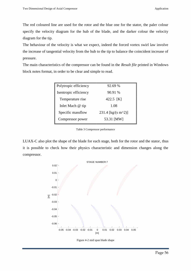
The main characteristics of the compressor can be found in the Result file printed in Windows
block notes format, in order to be clear and simple to read.
Polytropic efficiency 92.69 %
Isentropic efficiency 90.91 %
Temperature rise 422.5 [K]
Inlet Mach @ tip 1.08
Specific massflow 231.4 [kg/(s m^2)]
Compressor power 53.31 [MW]
Table 3 Compressor performance
LUAX-C also plot the shape of the blade for each stage, both for the rotor and the stator, thus
it is possible to check how their physics characteristic and dimension changes along the
compressor.
Figure 4-2 mid span blade shape
-0.05 -0.04 -0.03 -0.02 -0.01 0 0.01 0.02 0.03 0.04 0.05
-0.06
-0.05
-0.04
-0.03
-0.02
-0.01
0
0.01
0.02
[m]
[m]
STAGE NUMBER:7

Two Dimensional Design of Axial Compressor Application
Page 57
Another plot permitted by this new version of LUAX-C is the behaviour of the blade along its
span both for the rotor and the stator.
Rotating the view allow to have a better idea of the influence of the chosen swirl vortex on the
blade shape.
All the results have been confronted with literature, the behaviour of the velocity from the hub
to the tip for each swirl law, match with the existing dates (Aungier, 2003) at same initial
parameters.
-0.010
0.01
-0.02
0
0.02
0.35
0.36
0.37
0.38
0.39
0.4
0.41
0.42
0.43
0.44
[m]
Rotor Shape for Stage Number:7
[m][m] -5 0 5
x 10-3
-0.010
0.01
0.36
0.37
0.38
0.39
0.4
0.41
0.42
0.43
0.44
[m]
Stator Shape for Stage Number:7
[m][m]

Two Dimensional Design of Axial Compressor User’s Guide
Page 58
CHAPTER 5 USER’S GUIDE
In order to permit the choice of the swirl law and the new compressor type needed for the
design of the compressor, and the plot of the blade shape, the pre-existing GUI, Graphic User
Interface, has been modified.
When constant exit hut tip ratio is select, C_OGV window appears, and the Axial Velocity
Ratio one disappear because now is useless.
Furthermore choosing the General Whirl Distribution, the window for the pick of the n values
come into view, consent to select the desire swirl law (Figure 5-1).
Another extension make is the chance to do another bleed, improving the control on stall.
To start the calculation, after that all the parameters has been chosen, clicking on Create Data
File the input file will be created in a text file form where is also possible to change all the
dates.
Figure 5-1 LUAX-C Main Window

Two Dimensional Design of Axial Compressor User’s Guide
Page 59
Now is possible to start the calculation, selecting the RUN button, once all the loop are
terminated, both the shape of the flow path and the velocity diagrams appears; the duration of
this process can take some minutes, it depends from the performance of the calculator.
The Open Result File button open a Windows note file that contains all the result, from the
first stage to the OGV.
Two new buttons have been added, Blade Path Graph, which plot the rotor and the stator
airfoil at the mid-span, together for each stages, and Blade Hub to Tip Shape, which plot the
blade shape in the three positions.
Figure 5-2 Complete run window

Two Dimensional Design of Axial Compressor Bibliography
Page 60
Bibliography
Aungier, R. H. (2003). Axial-Flow Compressor. The American Society of Mechanical Engineers.
Berdanier, R. A. (n.d.). Hub Leakage Flow Research in Axial Compressors: A Literature Review.
Purdue University.
Bhaskar, R., & Pradeep, A. M. (n.d.). Turbomachinery Aerodynamics.
Bitterlich, W., Ausmeier, S., & Ulrich, L. (2002). Gasturbinen und Gasturbinenanlangen.
Teubner.
Boyce, M. P. (2011). Gas Turbine Engineering Handbook. Butterworth-Heinemann.
Chen, G.-T. (1991). Vortical structures in turbomachinery tip clearance flows. Massachusetts
Institute of Technology.
Dixon, S., & Hall, C. (2010). Fluid Mechanics and Thermodynamics of Turbomachiney.
Elsevier.
Falck, N. (2008). Axial Flow Compressor Mean Line Design. Lund.
Horlock, J. (1958). Axial Flow Compressor. Butterworth .
Johnson, & Bullock. (1965). Aerodynamic Design of Axial Flow Compressors. NASA SP 36.
Saravanamuttoo, H., Rogers, G., Cohen, H., & Straznicky, P. (2009). Gas Turbine Theory.
Pearson Education.
Schobeiri, M. T. (2012). Turbomachinery Flow Physics and Dynamic Performance. Springer.
Seppo, A. K. (2011). Principles of Turbomachinery. Hoboken, New Jersey: John Wiley & Sons.
Wisler, D. (1985). Aerodynamic Effects on Tip Clearance, Shrouds, Leakage Flow, Casing
Treatment and Trenching in Compressor Design. Von Karman Institute.
Xianjun, Y., Zhibo, Z., & Baojie, L. (2012). The evolution of the flow topologies of 3D
separations in the stator passage.

Two Dimensional Design of Axial Compressor Appendix
Page 61
APPENDIX
A, Table of figures
FIGURE 1-1 PRESSURE RATIO INCREASE ALONG THE YEARS ...........................................................................................5
FIGURE 1-2 AXIAL AND RADIAL COMPRESSOR ...............................................................................................................5
FIGURE 1-3 COMPARISON OF AXIAL CENTRIFUGAL CHARACTERISTIC CURVES (DRESSER-RAND) ..................................6
FIGURE 1-4 BLADE NOMENCLATURE ..............................................................................................................................7
FIGURE 1-5 DRAG AND LIFT FORCES ..............................................................................................................................8
FIGURE 1-6 LIFT AND DRAG COEFFICIENT .....................................................................................................................9
FIGURE 1-7 ROTATING STALL ....................................................................................................................................... 10
FIGURE 1-8 TIP CLEARANCE FLOW (BERDANIER) ......................................................................................................... 11
FIGURE 1-9 EFFECTS OF THE INCREASED CLEARANCE ON THE PERFORMANCE (WISLER, 1985) ................................... 11
FIGURE 2-1 CHARACTERISTIC CURVES OF THE COMPRESSOR (JOHNSON & BULLOCK, 1965) ....................................... 16
FIGURE 2-2 RADIAL SHIFT OF STREAMLINES THROUGH A BLADE ROW (JOHNSON & BULLOCK, 1965) ......................... 17
FIGURE 2-3 BOUNDARY LAYER (JOHNSON & BULLOCK, 1965) ..................................................................................... 17
FIGURE 2-4 VELOCITY DISTRIBUTION AND FLOW SEPARATION (JOHNSON & BULLOCK, 1965) .................................... 18
FIGURE 2-5 RELATION BETWEEN ISENTROPIC EFFICIENCY , POLYTROPIC EFFICIENCY AND PRESSURE RATIO ................ 20
FIGURE 2-6 MOLLIER DIAGRAM ................................................................................................................................... 20
FIGURE 2-7 VELOCITY DIAGRAM IN A COMPRESSOR STAGE .......................................................................................... 21
FIGURE 2-8 INFLUENCE OF REACTION ON VELOCITY DIAGRAM (DIXON & HALL, 2010) ............................................. 23
FIGURE 2-9 COMPARISON OF ANALYSIS WITH RESULT FROM MEASURE ....................................................................... 24
FIGURE 2-10 FORCES ACTING ON A FLUID ELEMENT .................................................................................................... 24
FIGURE 2-11 ACTUATOR DISK THEORY (HORLOCK, 1958) ........................................................................................... 28
FIGURE 2-12 VELOCITY PERTURBATION IN THE ACTUATOR DISK (DIXON & HALL, 2010) ........................................... 29
FIGURE 2-13 3D FLOW STRUCTURE (XIANJUN, ZHIBO, & BAOJIE, 2012) ...................................................................... 30
FIGURE 2-14 EXAMPLE OF MASH .................................................................................................................................. 31
FIGURE 2-15 BOUNDARY LAYER .................................................................................................................................. 32
FIGURE 3-1 STRUCTURE OF THE ITERATIONS (FALCK, 2008) ........................................................................................ 34
FIGURE 3-2 LUAX-C LOOPS ........................................................................................................................................ 36
FIGURE 3-3 FLOW PATH BEHAVIOUR WITH NEW DESIGN .............................................................................................. 38
FIGURE 3-4 MATLAB PLOT OF A DOUBLE CIRCULAR ARC PROFILE ................................................................................ 53
FIGURE 4-1 FLOW PATH AND VELOCITY DIAGRAMS FROM THE HUB TO THE TIP ........................................................... 55
FIGURE 4-2 MID SPAN BLADE SHAPE ............................................................................................................................ 56
FIGURE 5-1 LUAX-C MAIN WINDOW ......................................................................................................................... 58

Two Dimensional Design of Axial Compressor Appendix
Page 62
FIGURE 5-2 COMPLETE RUN WINDOW .......................................................................................................................... 59

Two Dimensional Design of Axial Compressor Appendix
Page 63
B, Matlab code
B1, Forced vortex law
%##################################################################### %## ## %## Forced Vortex law ## %## ## %## Daniele Perrotti 2013 ## %## ## %## Lund University/Dept of Energy Sciences ## %## ## %#####################################################################
globalvariables %call for the global variables global i flow j
%########### Forced Vortex for compressor stages ##########
%########################################################## %############### Station 1 Forced Vortex law ############## %##########################################################
%C1_FV_hub
C_theta1_FV_hub(i)=Cm1(i)*((r_hub_1(i)/r_rms_1(i))*tand(Alpha1(i)));
%C_theta1 at the hub Cm1_FV_hub(i)=(1+2*((tand(Alpha1(i))^2*(1-
(r_hub_1(i)/r_rms_1(i))^2))))^0.5*Cm1(i); U1_FV_hub(i)=r_hub_1(i)*pi*RPM/30;
W_theta1_FV_hub(i) = U1_FV_hub(i)-C_theta1_FV_hub(i); Beta1_FV_hub(i) = atand(W_theta1_FV_hub(i)/Cm1_FV_hub(i));
W1_FV_hub(i) = Cm1_FV_hub(i)/cosd(Beta1_FV_hub(i));
%C1_FV_tip
C_theta1_FV_tip(i)=Cm1(i)*(r_tip_1(i)/r_rms_1(i))*tand(Alpha1(i));
%C_theta1 at the tip Cm1_FV_tip(i)=(1+2*((tand(Alpha1(i))^2*(1-
(r_tip_1(i)/r_rms_1(i))^2))))^0.5*Cm1(i); %Cm1 at the tip U1_FV_tip(i)=r_tip_1(i)*pi*RPM/30;
W_theta1_FV_tip(i) = U1_FV_tip(i)-C_theta1_FV_tip(i); Beta1_FV_tip(i) = atand(W_theta1_FV_tip(i)/Cm1_FV_tip(i));
W1_FV_tip(i) = Cm1_FV_tip(i)/cosd(Beta1_FV_tip(i));

Two Dimensional Design of Axial Compressor Appendix
Page 64
%################## Station 1 Forced Vortex Rotor inlet #################
%#### HUB
if i==1
Cm1_FV_hub(i) = Cm_in; Alpha1_FV_hub(i) = Alpha_in; else
Alpha1_FV_hub(i) = Alpha3_FV_hub(i-1); end
C1_FV_hub(i) = Cm1_FV_hub(i)/cosd(Alpha1_FV_hub(i));
%#### TIP
if i==1
Cm1_FV_tip(i) = Cm_in; Alpha1_FV_tip(i) = Alpha_in; else
Alpha1_FV_tip(i) = Alpha3_FV_tip(i-1); end
C1_FV_tip(i) = Cm1_FV_tip(i)/cosd(Alpha1_FV_tip(i));
%################ Station 1 Forced Vortex total properties ##############
%#### HUB if i==1 % The first stage P01_FV_hub(i) = P0_in; T01_FV_hub(i) = T0_in; [P, T, H, S, Cp, rho, Visc, lambda, kappa, R, a, crit, FARsto, LHV,
y_SO2, y_H2O, y_CO2, y_N2, y_O2, y_Ar,
y_He]=state('PT',P01_FV_hub(i),T01_FV_hub(i),0,1); H01_FV_hub(i) = H; % S01(i) = S; % S1(i) = S; else P01_FV_hub(i) = P03_FV_hub(i-1); T01_FV_hub(i) = T03_FV_hub(i-1); H01_FV_hub(i) = H03_FV_hub(i-1); % S01(i) = S3(i-1); % S1(i) = S3(i-1); end
%#### TIP if i==1 % The first stage P01_FV_tip(i) = P0_in; T01_FV_tip(i) = T0_in; [P, T, H, S, Cp, rho, Visc, lambda, kappa, R, a, crit, FARsto, LHV,
y_SO2, y_H2O, y_CO2, y_N2, y_O2, y_Ar,
y_He]=state('PT',P01_FV_tip(i),T01_FV_tip(i),0,1); H01_FV_tip(i) = H; % S01(i) = S01; % S1(i) = S1;

Two Dimensional Design of Axial Compressor Appendix
Page 65
else P01_FV_tip(i) = P03_FV_tip(i-1); T01_FV_tip(i) = T03_FV_tip(i-1); H01_FV_tip(i) = H03_FV_tip(i-1); % S01(i) = S3(i-1); % S1(i) = S3(i-1); end %################# Station 1 FV static properties ############
%######## at the Hub
H1_FV_hub(i) = H01(i)-(C1_FV_hub(i)^2)/2; % Static enthalpy at rotor inlet
FV
[P, T, H, S, Cp, rho, Visc, lambda, kappa, R, a, crit, FARsto, LHV, y_SO2,
y_H2O, y_CO2, y_N2, y_O2, y_Ar, y_He]=state('HS',H1_FV_hub(i),S1(i),0,1); P1_FV_hub(i) = P; T1_FV_hub(i) = T; Cp1_FV_hub(i) = Cp; rho1_FV_hub(i) = rho; Visc1_FV_hub(i) = Visc; kappa1_FV_hub(i) = kappa; a1_FV_hub(i) = a;
MW1_FV_hub(i) = W1_FV_hub(i)/a1_FV_hub(i); % Station 1 relative Mach
FV_hub
MCm1_FV_hub(i) = Cm1_FV_hub(i)/a1_FV_hub(i); % Relative inlet meridional
Mach FV_hub
%####### at the Tip
H1_FV_tip(i) = H01(i)-(C1_FV_tip(i)^2)/2; % Static enthalpy at rotor inlet
FV
[P, T, H, S, Cp, rho, Visc, lambda, kappa, R, a, crit, FARsto, LHV, y_SO2,
y_H2O, y_CO2, y_N2, y_O2, y_Ar, y_He]=state('HS',H1_FV_tip(i),S1(i),0,1); P1_FV_tip(i) = P; T1_FV_tip(i) = T; Cp1_FV_tip(i) = Cp; rho1_FV_tip(i) = rho; Visc1_FV_tip(i) = Visc; kappa1_FV_tip(i) = kappa; a1_FV_tip(i) = a;
MW1_FV_tip(i) = W1_FV_tip(i)/a1_FV_tip(i); % Station 1 relative Mach
FV_tip
MCm1_FV_tip(i) = Cm1_FV_tip(i)/a1_FV_tip(i); % Relative inlet meridional
Mach FV_tip
%############# Station 1 FV relative properties ##############
%######## at the Hub
H01_rel_FV_hub(i) = H1_FV_hub(i)+ (W1_FV_hub(i)^2)/2; % Relative total
enthalpy

Two Dimensional Design of Axial Compressor Appendix
Page 66
[P, T, H, S, Cp, rho, Visc, lambda, kappa, R, a, crit, FARsto, LHV, y_SO2,
y_H2O, y_CO2, y_N2, y_O2, y_Ar,
y_He]=state('HS',H01_rel_FV_hub(i),S1(i),0,1); P01_rel_FV_hub(i) = P; T01_rel_FV_hub(i) = T;
I1_FV_hub(i) = H1_FV_hub(i)+(W1_FV_hub(i)^2)/2-(U1_FV_hub(i)^2)/2; %
Station 1 rothalpy at the hub
%####### at the Tip
H01_rel_FV_tip(i) = H1_FV_tip(i)+ (W1_FV_tip(i)^2)/2; % Relative total
enthalpy at the tip [P, T, H, S, Cp, rho, Visc, lambda, kappa, R, a, crit, FARsto, LHV, y_SO2,
y_H2O, y_CO2, y_N2, y_O2, y_Ar,
y_He]=state('HS',H01_rel_FV_tip(i),S1(i),0,1); P01_rel_FV_tip(i) = P; T01_rel_FV_tip(i) = T;
I1_FV_tip(i) = H1_FV_tip(i)+(W1_FV_tip(i)^2)/2-(U1_FV_tip(i)^2)/2; %
Station 1 rothalpy at the tip
%################################################## %############### Station 2 Forced Vortex law ###### %##################################################
% C2_FV_hub
C_theta2_FV_hub(i)=Cm2(i)*(tand(Alpha1(i))*(r_hub_2(i)/r_rms_2(i))+(PSI(j,i
)/(Cm2(i)/U2(i)))); Cm2_FV_hub(i)=Cm2(i)*((1+2*((tand(Alpha1(i))^2)*(1-
(r_hub_2(i)/r_rms_2(i))^2))-
4*(tand(Alpha1(i))*(PSI(j,i)/(Cm2(i)/U2(i)))*log(r_hub_2(i)/r_rms_2(i)))))^
0.5;
U2_FV_hub(i)=r_hub_2(i)*pi*RPM/30;
W_theta2_FV_hub(i) = U2_FV_hub(i)-C_theta2_FV_hub(i); C2_FV_hub(i) = (Cm2_FV_hub(i)^2+C_theta2_FV_hub(i)^2)^0.5; W2_FV_hub(i) = (Cm2_FV_hub(i)^2+W_theta2_FV_hub(i)^2)^0.5; Alpha2_FV_hub(i) = atand(C_theta2_FV_hub(i)/Cm2_FV_hub(i)); Beta2_FV_hub(i) = atand(W_theta2_FV_hub(i)/Cm2_FV_hub(i));
% C2_FV_tip
C_theta2_FV_tip(i)=Cm2(i)*(tand(Alpha1(i))*(r_tip_2(i)/r_rms_2(i))+(PSI(j,i
)/(Cm2(i)/U2(i)))); Cm2_FV_tip(i)=Cm2(i)*((1+2*((tand(Alpha1(i))^2)*(1-
(r_tip_2(i)/r_rms_2(i))^2))-
4*(tand(Alpha1(i))*(PSI(j,i)/(Cm2(i)/U2(i)))*log(r_tip_2(i)/r_rms_2(i)))))^
0.5;
U2_FV_tip(i)=r_tip_2(i)*pi*RPM/30;
W_theta2_FV_tip(i) = U2_FV_tip(i)-C_theta2_FV_tip(i);

Two Dimensional Design of Axial Compressor Appendix
Page 67
C2_FV_tip(i) = (Cm2_FV_tip(i)^2+C_theta2_FV_tip(i)^2)^0.5; W2_FV_tip(i) = (Cm2_FV_tip(i)^2+W_theta2_FV_tip(i)^2)^0.5; Alpha2_FV_tip(i) = atand(C_theta2_FV_tip(i)/Cm2_FV_tip(i)); Beta2_FV_tip(i) = atand(W_theta2_FV_tip(i)/Cm2_FV_tip(i));
%########## Station 2 FV static properties ###########
%##### at the hub
S2(i) = S1(i)+dS21(i);
I2_FV_hub(i) = I1_FV_hub(i); %I.e. constant rothalpy through a rotor
H2_FV_hub(i) = I2_FV_hub(i)-(W2_FV_hub(i)^2)/2+(U2_FV_hub(i)^2)/2;
[P, T, H, S, Cp, rho, Visc, lambda, kappa, R, a, crit, FARsto, LHV, y_SO2,
y_H2O, y_CO2, y_N2, y_O2, y_Ar, y_He] = state('HS',
H2_FV_hub(i),S2(i),0,1); P2_FV_hub(i) = P; T2_FV_hub(i) = T; Cp2_FV_hub(i) = Cp; rho2_FV_hub(i) = rho; Visc2_FV_hub(i) = Visc; kappa2_FV_hub(i) = kappa; a2_FV_hub(i) = a;
MC2_FV_hub(i) = C2_FV_hub(i)/a2_FV_hub(i); % Absolute inlet Mach FV_hub#
MCm2_FV_hub(i) = Cm2_FV_hub(i)/a2_FV_hub(i); % Relative inlet meridional
Mach FV_hub#
%#### at the tip S2(i) = S1(i)+dS21(i);
I2_FV_tip(i) = I1_FV_tip(i); %I.e. constant rothalpy through a rotor
H2_FV_tip(i) = I2_FV_tip(i)-(W2_FV_tip(i)^2)/2+(U2_FV_tip(i)^2)/2;
[P, T, H, S, Cp, rho, Visc, lambda, kappa, R, a, crit, FARsto, LHV, y_SO2,
y_H2O, y_CO2, y_N2, y_O2, y_Ar, y_He] = state('HS',H2_FV_tip(i),S2(i),0,1); P2_FV_tip(i) = P; T2_FV_tip(i) = T; Cp2_FV_tip(i) = Cp; rho2_FV_tip(i) = rho; Visc2_FV_tip(i) = Visc; kappa2_FV_tip(i) = kappa; a2_FV_tip(i) = a;
MC2_FV_tip(i) = C2_FV_tip(i)/a2_FV_tip(i); % Absolute inlet Mach FV_tip
MCm2_FV_tip(i) = Cm2_FV_tip(i)/a2_FV_tip(i); % Relative inlet meridional
Mach FV_tip
%############# Station 2 FV relative properties ##############

Two Dimensional Design of Axial Compressor Appendix
Page 68
%##### at the hub
H02_rel_FV_hub(i) = H2_FV_hub(i)+ (W2_FV_hub(i)^2)/2; % Relative total
enthalpy [P, T, H, S, Cp, rho, Visc, lambda, kappa, R, a, crit, FARsto, LHV, y_SO2,
y_H2O, y_CO2, y_N2, y_O2, y_Ar,
y_He]=state('HS',H02_rel_FV_hub(i),S2(i),0,1); P02_rel_FV_hub(i) = P; T02_rel_FV_hub(i) = T;
%##### at the tip
H02_rel_FV_tip(i) = H2_FV_tip(i)+ (W2_FV_tip(i)^2)/2; % Relative total
enthalpy [P, T, H, S, Cp, rho, Visc, lambda, kappa, R, a, crit, FARsto, LHV, y_SO2,
y_H2O, y_CO2, y_N2, y_O2, y_Ar,
y_He]=state('HS',H02_rel_FV_tip(i),S2(i),0,1); P02_rel_FV_tip(i) = P; T02_rel_FV_tip(i) = T;
%########### Station 2 FV total properties ###########
%##### at the hub
H02_FV_hub(i) = H2_FV_hub(i)+(C2_FV_hub(i)^2)/2; % Exit total enthalpy [P, T, H, S, Cp, rho, Visc, lambda, kappa, R, a, crit, FARsto, LHV, y_SO2,
y_H2O, y_CO2, y_N2, y_O2, y_Ar, y_He] =
state('HS',H02_FV_hub(i),S2(i),0,1); P02_FV_hub(i) = P; T02_FV_hub(i) = T;
%##### at the tip
H02_FV_tip(i) = H2_FV_tip(i)+(C2_FV_tip(i)^2)/2; % Exit total enthalpy [P, T, H, S, Cp, rho, Visc, lambda, kappa, R, a, crit, FARsto, LHV, y_SO2,
y_H2O, y_CO2, y_N2, y_O2, y_Ar, y_He] =
state('HS',H02_FV_tip(i),S2(i),0,1); P02_FV_tip(i) = P; T02_FV_tip(i) = T;
%######## deHaller number Forced Vortex law rtr
%##### at the hub dH_rtr_FV_hub(i)=W2_FV_hub(i)/W1_FV_hub(i);
%#### at the tip dH_rtr_FV_tip(i)=W2_FV_tip(i)/W1_FV_tip(i);
%################################################## %############Station 3 Forced Vortex law########### %##################################################
% C3_FV_hub C_theta3_FV_hub(i)=Cm3(i)*(r_hub_3(i)/r_rms_3(i))*tand(Alpha1(i));
%C_theta3 at the hub

Two Dimensional Design of Axial Compressor Appendix
Page 69
Cm3_FV_hub(i)=Cm3(i)*sqrt(1+2*tand(Alpha1(i))^2*(1-
(r_hub_3(i)/r_rms_3(i))^2)); %Cm3 at the hub Alpha3_FV_hub(i) = atand(C_theta3_FV_hub(i)/Cm3_FV_hub(i)); C3_FV_hub(i) = Cm3_FV_hub(i)/cosd(Alpha3_FV_hub(i));
% C3_FV_tip C_theta3_FV_tip(i)=Cm3(i)*(r_tip_3(i)/r_rms_3(i))*tand(Alpha1(i));%C_theta3
at the tip Cm3_FV_tip(i)=Cm3(i)*sqrt(1+2*tand(Alpha1(i))^2*(1-
(r_tip_3(i)/r_rms_3(i))^2)); %Cm3 at the tip Alpha3_FV_tip(i) = atand(C_theta3_FV_tip(i)/Cm3_FV_tip(i)); C3_FV_tip(i) = Cm3_FV_tip(i)/cosd(Alpha3_FV_tip(i));
%########### Station 3 FV static properties ##########
%#### HUB
H03_FV_hub(i) = H02_FV_hub(i); % Constant total enthalpy through the stator H3_FV_hub(i) = H03_FV_hub(i)-(C3_FV_hub(i)^2)/2; S3(i) = S2(i)+dS32(i); [P, T, H, S, Cp, rho, Visc, lambda, kappa, R, a, crit, FARsto, LHV, y_SO2,
y_H2O, y_CO2, y_N2, y_O2, y_Ar, y_He]=state('HS',H3_FV_hub(i),S3(i),0,1); P3_FV_hub(i) = P; T3_FV_hub(i) = T; Cp3_FV_hub(i) = Cp; rho3_FV_hub(i) = rho; Visc3_FV_hub(i) = Visc; kappa3_FV_hub(i) = kappa; a3_FV_hub(i) = a;
MC3_FV_hub(i) = C3_FV_hub(i)/a3_FV_hub(i);% Absolute inlet Mach FV_hub #
MCm3_FV_hub(i) = Cm3_FV_hub(i)/a3_FV_hub(i);% Relative inlet meridional
Mach FV_hub #
%#### TIP
H03_FV_tip(i) = H02_FV_tip(i); % Constant total enthalpy through the stator H3_FV_tip(i) = H03_FV_tip(i)-(C3_FV_tip(i)^2)/2; S3(i) = S2(i)+dS32(i); [P, T, H, S, Cp, rho, Visc, lambda, kappa, R, a, crit, FARsto, LHV, y_SO2,
y_H2O, y_CO2, y_N2, y_O2, y_Ar, y_He]=state('HS',H3_FV_tip(i),S3(i),0,1); P3_FV_tip(i) = P; T3_FV_tip(i) = T; Cp3_FV_tip(i) = Cp; rho3_FV_tip(i) = rho; Visc3_FV_tip(i) = Visc; kappa3_FV_tip(i) = kappa; a3_FV_tip(i) = a;
MC3_FV_tip(i) = C3_FV_hub(i)/a3_FV_hub(i);% Absolute inlet Mach FV_hub #
MCm3_FV_tip(i) = Cm3_FV_hub(i)/a3_FV_hub(i);% Relative inlet meridional
Mach FV_hub #
%############ Station 3 FV total properties ##########
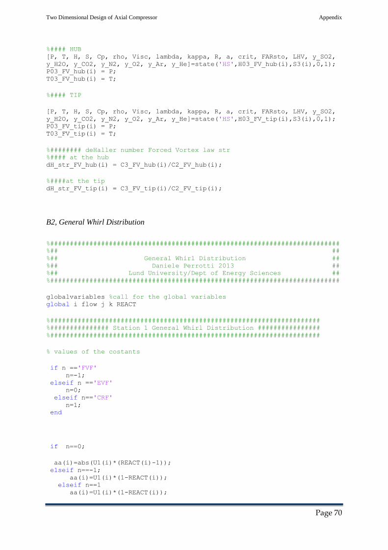
Two Dimensional Design of Axial Compressor Appendix
Page 70
%#### HUB [P, T, H, S, Cp, rho, Visc, lambda, kappa, R, a, crit, FARsto, LHV, y_SO2,
y_H2O, y_CO2, y_N2, y_O2, y_Ar, y_He]=state('HS',H03_FV_hub(i),S3(i),0,1); P03_FV_hub(i) = P; T03_FV_hub(i) = T;
%#### TIP
[P, T, H, S, Cp, rho, Visc, lambda, kappa, R, a, crit, FARsto, LHV, y_SO2,
y_H2O, y_CO2, y_N2, y_O2, y_Ar, y_He]=state('HS',H03_FV_tip(i),S3(i),0,1); P03_FV_tip(i) = P; T03_FV_tip(i) = T;
%######## deHaller number Forced Vortex law str %#### at the hub dH_str_FV_hub(i) = C3_FV_hub(i)/C2_FV_hub(i);
%####at the tip dH_str_FV_tip(i) = C3_FV_tip(i)/C2_FV_tip(i);
B2, General Whirl Distribution
%########################################################################## %## ## %## General Whirl Distribution ## %## Daniele Perrotti 2013 ## %## Lund University/Dept of Energy Sciences ## %##########################################################################
globalvariables %call for the global variables global i flow j k REACT
%##################################################################### %############### Station 1 General Whirl Distribution ################ %#####################################################################
% values of the costants
if n =='FVF' n=-1; elseif n =='EVF' n=0; elseif n=='CRF' n=1; end
if n==0;
aa(i)=abs(U1(i)*(REACT(i)-1)); elseif n==-1; aa(i)=U1(i)*(1-REACT(i)); elseif n==1 aa(i)=U1(i)*(1-REACT(i));

Two Dimensional Design of Axial Compressor Appendix
Page 71
end
bb(i)=1/2*(PSI(j,i)*U1(i));
%#### C_theta1 FREE VORTEX LAW C_theta1_FREEV_hub(i)=aa(i)*(r_hub_1(i)/r_rms_1(i))^(n)-
bb(i)/(r_hub_1(i)/r_rms_1(i)); C_theta1_FREEV_tip(i)=aa(i)*(r_tip_1(i)/r_rms_1(i))^(n)-
bb(i)/(r_tip_1(i)/r_rms_1(i));
%#### Cm1 FREE VORTEX LAW
if n==-1 % Cm1_FREEV_hub Cm1_FREEV_hub(i)=Cm1(i); Cm1_FREEV_tip(i)=Cm1(i); elseif n==0
% Cm1_FREEV_hub Cm1_FREEV_hub(i)=sqrt(Cm1(i)^2-
(2*(aa(i)^2*log(r_hub_1(i)/r_rms_1(i))+aa(i)*bb(i)*(1/(r_hub_1(i)/r_rms_1(i
))-1)))); % Cm1_FREEV_tip Cm1_FREEV_tip(i)=sqrt(Cm1(i)^2-
(2*(aa(i)^2*log(r_tip_1(i)/r_rms_1(i))+aa(i)*bb(i)*(1/(r_tip_1(i)/r_rms_1(i
))-1)))); elseif n==1
% Cm1_FREEV_hub
Cm1_FREEV_hub(i)=sqrt(Cm1(i)^2+(4*aa(i)*bb(i)*log(r_hub_1(i)/r_rms_1(i))-
2*aa(i)^2*((r_hub_1(i)/r_rms_1(i))^2-1))); % Cm1_FREEV_tip
Cm1_FREEV_tip(i)=sqrt(Cm1(i)^2+(4*aa(i)*bb(i)*log(r_tip_1(i)/r_rms_1(i))-
2*aa(i)^2*((r_tip_1(i)/r_rms_1(i))^2-1)));
end
%W1_FREEV_hub U1_FREEV_hub(i)=r_hub_1(i)*pi*RPM/30;
W_theta1_FREEV_hub(i) = U1_FREEV_hub(i)-C_theta1_FREEV_hub(i); Beta1_FREEV_hub(i) = atand(W_theta1_FREEV_hub(i)/Cm1_FREEV_hub(i)); W1_FREEV_hub(i) = Cm1_FREEV_hub(i)/cosd(Beta1_FREEV_hub(i));
%W1_FREEV_tip U1_FREEV_tip(i)=r_tip_1(i)*pi*RPM/30;
W_theta1_FREEV_tip(i) = U1_FREEV_tip(i)-C_theta1_FREEV_tip(i); Beta1_FREEV_tip(i) = atand(W_theta1_FREEV_tip(i)/Cm1_FREEV_tip(i)); W1_FREEV_tip(i) = Cm1_FREEV_tip(i)/cosd(Beta1_FREEV_tip(i));
% ################## Station 1 General Whirl Distribution Rotor inlet ####

Two Dimensional Design of Axial Compressor Appendix
Page 72
%#### HUB
if i==1 Cm1_FREEV_hub(i) = Cm_in; Alpha1_FREEV_hub(i) = Alpha_in;
else Alpha1_FREEV_hub(i) = Alpha3_FREEV_hub(i-1);
end
C1_FREEV_hub(i) = Cm1_FREEV_hub(i)/cosd(Alpha1_FREEV_hub(i));
%#### TIP
if i==1
Cm1_FREEV_tip(i) = Cm_in; Alpha1_FREEV_tip(i) = Alpha_in; else
Alpha1_FREEV_tip(i) = Alpha3_FREEV_tip(i-1); end
C1_FREEV_tip(i) = Cm1_FREEV_tip(i)/cosd(Alpha1_FREEV_tip(i));
%################ Station 1 General Whirl Distribution total properties
##############
%#### HUB if i==1 % The first stage P01_FREEV_hub(i) = P0_in; T01_FREEV_hub(i) = T0_in; [P, T, H, S, Cp, rho, Visc, lambda, kappa, R, a, crit, FARsto, LHV,
y_SO2, y_H2O, y_CO2, y_N2, y_O2, y_Ar,
y_He]=state('PT',P01_FREEV_hub(i),T01_FREEV_hub(i),0,1); H01_FREEV_hub(i) = H; % S01(i) = S; % S1(i) = S; else P01_FREEV_hub(i) = P03_FREEV_hub(i-1); T01_FREEV_hub(i) = T03_FREEV_hub(i-1); H01_FREEV_hub(i) = H03_FREEV_hub(i-1); % S01(i) = S3(i-1); % S1(i) = S3(i-1); end
%#### TIP if i==1 % The first stage P01_FREEV_tip(i) = P0_in; T01_FREEV_tip(i) = T0_in; [P, T, H, S, Cp, rho, Visc, lambda, kappa, R, a, crit, FARsto, LHV,
y_SO2, y_H2O, y_CO2, y_N2, y_O2, y_Ar,
y_He]=state('PT',P01_FREEV_tip(i),T01_FREEV_tip(i),0,1); H01_FREEV_tip(i) = H; % S01(i) = S; % S1(i) = S; else

Two Dimensional Design of Axial Compressor Appendix
Page 73
P01_FREEV_tip(i) = P03_FREEV_tip(i-1); T01_FREEV_tip(i) = T03_FREEV_tip(i-1); H01_FREEV_tip(i) = H03_FREEV_tip(i-1); % S01(i) = S3(i-1); % S1(i) = S3(i-1); end
%################# Station 1 General Whirl Distribution static properties
############
%######## at the Hub
H1_FREEV_hub(i) = H01(i)-(C1_FREEV_hub(i)^2)/2; % Static enthalpy at rotor
inlet FREEV
[P, T, H, S, Cp, rho, Visc, lambda, kappa, R, a, crit, FARsto, LHV, y_SO2,
y_H2O, y_CO2, y_N2, y_O2, y_Ar,
y_He]=state('HS',H1_FREEV_hub(i),S1(i),0,1); P1_FREEV_hub(i) = P; T1_FREEV_hub(i) = T; Cp1_FREEV_hub(i) = Cp; rho1_FREEV_hub(i) = rho; Visc1_FREEV_hub(i) = Visc; kappa1_FREEV_hub(i) = kappa; a1_FREEV_hub(i) = a;
MW1_FREEV_hub(i) = W1_FREEV_hub(i)/a1_FREEV_hub(i); % Station 1 relative
Mach FREEV_hub
MCm1_FREEV_hub(i) = Cm1_FREEV_hub(i)/a1_FREEV_hub(i); % Relative inlet
meridional Mach FREEV_hub
%####### at the Tip
H1_FREEV_tip(i) = H01(i)-(C1_FREEV_tip(i)^2)/2; % Static enthalpy at rotor
inlet FREEV
[P, T, H, S, Cp, rho, Visc, lambda, kappa, R, a, crit, FARsto, LHV, y_SO2,
y_H2O, y_CO2, y_N2, y_O2, y_Ar,
y_He]=state('HS',H1_FREEV_tip(i),S1(i),0,1); P1_FREEV_tip(i) = P; T1_FREEV_tip(i) = T; Cp1_FREEV_tip(i) = Cp; rho1_FREEV_tip(i) = rho; Visc1_FREEV_tip(i) = Visc; kappa1_FREEV_tip(i) = kappa; a1_FREEV_tip(i) = a;
MW1_FREEV_tip(i) = W1_FREEV_tip(i)/a1_FREEV_tip(i); % Station 1 relative
Mach FREEV_tip
MCm1_FREEV_tip(i) = Cm1_FREEV_tip(i)/a1_FREEV_tip(i); % Relative inlet
meridional Mach FREEV_tip
%############# Station 1 General Whirl Distribution relative properties
##############
%######## at the Hub

Two Dimensional Design of Axial Compressor Appendix
Page 74
H01_rel_FREEV_hub(i) = H1_FREEV_hub(i)+ (W1_FREEV_hub(i)^2)/2; % Relative
total enthalpy [P, T, H, S, Cp, rho, Visc, lambda, kappa, R, a, crit, FARsto, LHV, y_SO2,
y_H2O, y_CO2, y_N2, y_O2, y_Ar,
y_He]=state('HS',H01_rel_FREEV_hub(i),S1(i),0,1); P01_rel_FREEV_hub(i) = P; T01_rel_FREEV_hub(i) = T;
I1_FREEV_hub(i) = H1_FREEV_hub(i)+(W1_FREEV_hub(i)^2)/2-
(U1_FREEV_hub(i)^2)/2; % Station 1 rothalpy at the hub
%####### at the Tip
H01_rel_FREEV_tip(i) = H1_FREEV_tip(i)+ (W1_FREEV_tip(i)^2)/2; % Relative
total enthalpy at the tip [P, T, H, S, Cp, rho, Visc, lambda, kappa, R, a, crit, FARsto, LHV, y_SO2,
y_H2O, y_CO2, y_N2, y_O2, y_Ar,
y_He]=state('HS',H01_rel_FREEV_tip(i),S1(i),0,1); P01_rel_FREEV_tip(i) = P; T01_rel_FREEV_tip(i) = T;
I1_FREEV_tip(i) = H1_FREEV_tip(i)+(W1_FREEV_tip(i)^2)/2-
(U1_FREEV_tip(i)^2)/2; % Station 1 rothalpy at the tip
%############ Station 1 Reaction variation across the radius ##############
if n==-1 REACT1_FREEV_hub(i)=1-(1-REACT(i))/((r_hub_rtr(i)/r_rms_1(i))^2); REACT1_FREEV_tip(i)=1-(1-REACT(i))/((r_tip_rtr(i)/r_rms_1(i))^2); elseif n==0 REACT1_FREEV_hub(i)=1+(1-REACT(i))*(1-
2/(r_hub_rtr(i)/r_rms_1(i))); REACT1_FREEV_tip(i)=1+(1-REACT(i))*(1-
2/(r_tip_rtr(i)/r_rms_1(i))); elseif n==1 REACT1_FREEV_hub(i)=1-(1-REACT(i))*(1-
2*log(r_hub_rtr(i)/r_rms_1(i))); REACT1_FREEV_tip(i)=1-(1-REACT(i))*(1-
2*log(r_tip_rtr(i)/r_rms_1(i))); end
%#############à####################################################### %###################### Station 2 General Whirl Distribution ######### %#####################################################################
%#### C_theta2 General Whirl Distribution C_theta2_FREEV_hub(i)=aa(i)*(r_hub_2(i)/r_rms_2(i))^(n)+bb(i)/(r_hub_2(i)/r
_rms_2(i)); C_theta2_FREEV_tip(i)=aa(i)*(r_tip_2(i)/r_rms_2(i))^(n)+bb(i)/(r_tip_2(i)/r
_rms_2(i));
%#### Cm2 General Whirl Distribution if n==-1 Cm2_FREEV_hub(i)=Cm2(i); Cm2_FREEV_tip(i)=Cm2(i); elseif n==0

Two Dimensional Design of Axial Compressor Appendix
Page 75
Cm2_FREEV_hub(i)=sqrt(Cm2(i)^2-
(2*(aa(i)^2*log(r_hub_2(i)/r_rms_2(i))-
aa(i)*bb(i)*(1/(r_hub_2(i)/r_rms_2(i))-1)))); Cm2_FREEV_tip(i)=sqrt(Cm2(i)^2-
(2*(aa(i)^2*log(r_tip_2(i)/r_rms_2(i))-
aa(i)*bb(i)*(1/(r_tip_2(i)/r_rms_2(i))-1)))); elseif n==1 Cm2_FREEV_hub(i)=sqrt(Cm2(i)^2-
4*aa(i)*bb(i)*log(r_hub_2(i)/r_rms_2(i))-
2*(aa(i)^2)*((r_hub_2(i)/r_rms_2(i))^2-1)); Cm2_FREEV_tip(i)=sqrt(Cm2(i)^2-
4*aa(i)*bb(i)*log(r_tip_2(i)/r_rms_2(i))-
2*(aa(i)^2)*((r_tip_2(i)/r_rms_2(i))^2-1)); end
%W2_FREEV_hub U2_FREEV_hub(i)=r_hub_2(i)*pi*RPM/30;
W_theta2_FREEV_hub(i) = U2_FREEV_hub(i)-C_theta2_FREEV_hub(i); Beta2_FREEV_hub(i) = atand(W_theta2_FREEV_hub(i)/Cm2_FREEV_hub(i)); W2_FREEV_hub(i) = Cm2_FREEV_hub(i)/cosd(Beta2_FREEV_hub(i));
%C2_FREEV_hub C2_FREEV_hub(i) = (Cm2_FREEV_hub(i)^2+C_theta2_FREEV_hub(i)^2)^0.5; Alpha2_FREEV_hub(i) = atand(C_theta2_FREEV_hub(i)/Cm2_FREEV_hub(i));
%W2_FREEV_tip U2_FREEV_tip(i)=r_tip_2(i)*pi*RPM/30;
W_theta2_FREEV_tip(i) = U2_FREEV_tip(i)-C_theta2_FREEV_tip(i); Beta2_FREEV_tip(i) = atand(W_theta2_FREEV_tip(i)/Cm2_FREEV_tip(i)); W2_FREEV_tip(i) = Cm2_FREEV_tip(i)/cosd(Beta2_FREEV_tip(i));
%C2_free_tip C2_FREEV_tip(i) = (Cm2_FREEV_tip(i)^2+C_theta2_FREEV_tip(i)^2)^0.5; Alpha2_FREEV_tip(i) = atand(C_theta2_FREEV_tip(i)/Cm2_FREEV_tip(i));
W2onW1_hub(i)=W2_FREEV_hub(i)/W1_FREEV_hub(i); W2onW1_tip(i)=W2_FREEV_tip(i)/W1_FREEV_tip(i); %########## Station 2 General Whirl Distribution static properties
###########
%##### at the hub
S2(i) = S1(i)+dS21(i);
I2_FREEV_hub(i) = I1_FREEV_hub(i); %I.e. constant rothalpy through a rotor
H2_FREEV_hub(i) = I2_FREEV_hub(i)-
(W2_FREEV_hub(i)^2)/2+(U2_FREEV_hub(i)^2)/2;
[P, T, H, S, Cp, rho, Visc, lambda, kappa, R, a, crit, FARsto, LHV, y_SO2,
y_H2O, y_CO2, y_N2, y_O2, y_Ar, y_He] = state('HS',
H2_FREEV_hub(i),S2(i),0,1); P2_FREEV_hub(i) = P; T2_FREEV_hub(i) = T; Cp2_FREEV_hub(i) = Cp;

Two Dimensional Design of Axial Compressor Appendix
Page 76
rho2_FREEV_hub(i) = rho; Visc2_FREEV_hub(i) = Visc; kappa2_FREEV_hub(i) = kappa; a2_FREEV_hub(i) = a;
MC2_FREEV_hub(i) = C2_FREEV_hub(i)/a2_FREEV_hub(i); % Absolute inlet Mach
FREEV_hub#
MCm2_FREEV_hub(i) = Cm2_FREEV_hub(i)/a2_FREEV_hub(i); % Relative inlet
meridional Mach FREEV_hub#
%#### at the tip S2(i) = S1(i)+dS21(i);
I2_FREEV_tip(i) = I1_FREEV_tip(i); %I.e. constant rothalpy through a rotor
H2_FREEV_tip(i) = I2_FREEV_tip(i)-
(W2_FREEV_tip(i)^2)/2+(U2_FREEV_tip(i)^2)/2;
[P, T, H, S, Cp, rho, Visc, lambda, kappa, R, a, crit, FARsto, LHV, y_SO2,
y_H2O, y_CO2, y_N2, y_O2, y_Ar, y_He] =
state('HS',H2_FREEV_tip(i),S2(i),0,1); P2_FREEV_tip(i) = P; T2_FREEV_tip(i) = T; Cp2_FREEV_tip(i) = Cp; rho2_FREEV_tip(i) = rho; Visc2_FREEV_tip(i) = Visc; kappa2_FREEV_tip(i) = kappa; a2_FREEV_tip(i) = a;
MC2_FREEV_tip(i) = C2_FREEV_tip(i)/a2_FREEV_tip(i); % Absolute inlet Mach
FREEV_tip
MCm2_FREEV_tip(i) = Cm2_FREEV_tip(i)/a2_FREEV_tip(i); % Relative inlet
meridional Mach FREEV_tip
%############# Station 2 General Whirl Distribution relative properties
##############
%##### at the hub
H02_rel_FREEV_hub(i) = H2_FREEV_hub(i)+ (W2_FREEV_hub(i)^2)/2; % Relative
total enthalpy [P, T, H, S, Cp, rho, Visc, lambda, kappa, R, a, crit, FARsto, LHV, y_SO2,
y_H2O, y_CO2, y_N2, y_O2, y_Ar,
y_He]=state('HS',H02_rel_FREEV_hub(i),S2(i),0,1); P02_rel_FREEV_hub(i) = P; T02_rel_FREEV_hub(i) = T;
%##### at the tip
H02_rel_FREEV_tip(i) = H2_FREEV_tip(i)+ (W2_FREEV_tip(i)^2)/2; % Relative
total enthalpy

Two Dimensional Design of Axial Compressor Appendix
Page 77
[P, T, H, S, Cp, rho, Visc, lambda, kappa, R, a, crit, FARsto, LHV, y_SO2,
y_H2O, y_CO2, y_N2, y_O2, y_Ar,
y_He]=state('HS',H02_rel_FREEV_tip(i),S2(i),0,1); P02_rel_FREEV_tip(i) = P; T02_rel_FREEV_tip(i) = T;
%########### Station 2 General Whirl Distribution total properties
###########
%##### at the hub
H02_FREEV_hub(i) = H2_FREEV_hub(i)+(C2_FREEV_hub(i)^2)/2; % Exit total
enthalpy [P, T, H, S, Cp, rho, Visc, lambda, kappa, R, a, crit, FARsto, LHV, y_SO2,
y_H2O, y_CO2, y_N2, y_O2, y_Ar, y_He] =
state('HS',H02_FREEV_hub(i),S2(i),0,1); P02_FREEV_hub(i) = P; T02_FREEV_hub(i) = T;
%##### at the tip
H02_FREEV_tip(i) = H2_FREEV_tip(i)+(C2_FREEV_tip(i)^2)/2; % Exit total
enthalpy [P, T, H, S, Cp, rho, Visc, lambda, kappa, R, a, crit, FARsto, LHV, y_SO2,
y_H2O, y_CO2, y_N2, y_O2, y_Ar, y_He] =
state('HS',H02_FREEV_tip(i),S2(i),0,1); P02_FREEV_tip(i) = P; T02_FREEV_tip(i) = T;
%######## deHaller number Free Vortex law rtr
%##### at the hub dH_rtr_FREEV_hub(i)=W2_FREEV_hub(i)/W1_FREEV_hub(i);
%#### at the tip dH_rtr_FREEV_tip(i)=W2_FREEV_tip(i)/W1_FREEV_tip(i);
%################################################## %############Station 3 General Whirl Distribution## %##################################################
%#### C_theta3 FREE VORTEX LAW C_theta3_FREEV_hub(i)=aa(i)*(r_hub_3(i)/r_rms_3(i))^(n)-
bb(i)/(r_hub_3(i)/r_rms_3(i)); C_theta3_FREEV_tip(i)=aa(i)*(r_tip_3(i)/r_rms_3(i))^(n)-
bb(i)/(r_tip_3(i)/r_rms_3(i));
%#### Cm3 FREE VORTEX LAW
if n==-1 % Cm3_FREEV_hub Cm3_FREEV_hub(i)=Cm3(i); % Cm1_FREEV_tip Cm3_FREEV_tip(i)=Cm3(i); elseif n==0 % Cm3_FREEV_hub Cm3_FREEV_hub(i)=sqrt(Cm3(i)^2-
(2*(aa(i)^2*log(r_hub_3(i)/r_rms_3(i))+aa(i)*bb(i)*(1/(r_hub_3(i)/r_rms_3(i
))-1))));

Two Dimensional Design of Axial Compressor Appendix
Page 78
% Cm3_FREEV_tip Cm3_FREEV_tip(i)=sqrt(Cm3(i)^2-
(2*(aa(i)^2*log(r_tip_3(i)/r_rms_3(i))+aa(i)*bb(i)*(1/(r_tip_3(i)/r_rms_3(i
))-1)))); elseif n==1 % Cm3_FREEV_hub
Cm3_FREEV_hub(i)=sqrt(Cm3(i)^2+(4*aa(i)*bb(i)*log(r_hub_3(i)/r_rms_3(i))-
2*aa(i)^2*((r_hub_3(i)/r_rms_3(i))^2-1))); % Cm3_FREEV_tip
Cm3_FREEV_tip(i)=sqrt(Cm3(i)^2+(4*aa(i)*bb(i)*log(r_tip_3(i)/r_rms_3(i))-
2*aa(i)^2*((r_tip_3(i)/r_rms_3(i))^2-1)));
end
% C and U FREE VORTEX
Alpha3_FREEV_hub(i) = atand(C_theta3_FREEV_hub(i)/Cm3_FREEV_hub(i)); C3_FREEV_hub(i) = Cm3_FREEV_hub(i)/cosd(Alpha3_FREEV_hub(i)); U3_FREEV_hub(i)=r_hub_3(i)*pi*RPM/30;
Alpha3_FREEV_tip(i) = atand(C_theta3_FREEV_tip(i)/Cm3_FREEV_tip(i)); C3_FREEV_tip(i) = Cm3_FREEV_tip(i)/cosd(Alpha3_FREEV_tip(i)); U3_FREEV_tip(i)=r_tip_3(i)*pi*RPM/30; C3onC2_hub(i)=C3_FREEV_hub(i)/C2_FREEV_hub(i); C3onC2_tip(i)=C3_FREEV_tip(i)/C2_FREEV_tip(i); Cm1onU1_hub(i)=Cm1_FREEV_hub(i)/U1(i); Cm1onU1_tip(i)=Cm1_FREEV_tip(i)/U1(i); Cm2onU2_hub(i)=Cm2_FREEV_hub(i)/U2(i); Cm2onU2_tip(i)=Cm2_FREEV_tip(i)/U2(i); W1onU1_hub(i)= W1_FREEV_hub(i)/U1(i); W1onU1_tip(i)= W1_FREEV_tip(i)/U1(i); W2onU1_hub(i)= W2_FREEV_hub(i)/U1(i); W2onU1_tip(i)= W2_FREEV_tip(i)/U1(i);
%########### Station 3 General Whirl Distribution static properties
##########
%#### HUB
H03_FREEV_hub(i) = H02_FREEV_hub(i); % Constant total enthalpy through the
stator H3_FREEV_hub(i) = H03_FREEV_hub(i)-(C3_FREEV_hub(i)^2)/2; S3(i) = S2(i)+dS32(i); [P, T, H, S, Cp, rho, Visc, lambda, kappa, R, a, crit, FARsto, LHV, y_SO2,
y_H2O, y_CO2, y_N2, y_O2, y_Ar,
y_He]=state('HS',H3_FREEV_hub(i),S3(i),0,1); P3_FREEV_hub(i) = P; T3_FREEV_hub(i) = T; Cp3_FREEV_hub(i) = Cp; rho3_FREEV_hub(i) = rho; Visc3_FREEV_hub(i) = Visc; kappa3_FREEV_hub(i) = kappa; a3_FREEV_hub(i) = a;
MC3_FREEV_hub(i) = C3_FREEV_hub(i)/a3_FREEV_hub(i);% Absolute inlet Mach
FREEV_hub #

Two Dimensional Design of Axial Compressor Appendix
Page 79
MCm3_FREEV_hub(i) = Cm3_FREEV_hub(i)/a3_FREEV_hub(i);% Relative inlet
meridional Mach FREEV_hub #
%#### TIP
H03_FREEV_tip(i) = H02_FREEV_tip(i); % Constant total enthalpy through the
stator H3_FREEV_tip(i) = H03_FREEV_tip(i)-(C3_FREEV_tip(i)^2)/2; S3(i) = S2(i)+dS32(i); [P, T, H, S, Cp, rho, Visc, lambda, kappa, R, a, crit, FARsto, LHV, y_SO2,
y_H2O, y_CO2, y_N2, y_O2, y_Ar,
y_He]=state('HS',H3_FREEV_tip(i),S3(i),0,1); P3_FREEV_tip(i) = P; T3_FREEV_tip(i) = T; Cp3_FREEV_tip(i) = Cp; rho3_FREEV_tip(i) = rho; Visc3_FREEV_tip(i) = Visc; kappa3_FREEV_tip(i) = kappa; a3_FREEV_tip(i) = a;
MC3_FREEV_tip(i) = C3_FREEV_hub(i)/a3_FREEV_hub(i);% Absolute inlet Mach
FREEV_hub #
MCm3_FREEV_tip(i) = Cm3_FREEV_hub(i)/a3_FREEV_hub(i);% Relative inlet
meridional Mach FREEV_hub #
%############ Station 3 General Whirl Distribution total properties
##########
%#### HUB [P, T, H, S, Cp, rho, Visc, lambda, kappa, R, a, crit, FARsto, LHV, y_SO2,
y_H2O, y_CO2, y_N2, y_O2, y_Ar,
y_He]=state('HS',H03_FREEV_hub(i),S3(i),0,1); P03_FREEV_hub(i) = P; T03_FREEV_hub(i) = T;
%#### TIP
[P, T, H, S, Cp, rho, Visc, lambda, kappa, R, a, crit, FARsto, LHV, y_SO2,
y_H2O, y_CO2, y_N2, y_O2, y_Ar,
y_He]=state('HS',H03_FREEV_tip(i),S3(i),0,1); P03_FREEV_tip(i) = P; T03_FREEV_tip(i) = T;
%######## deHaller number Forced Vortex law str %#### at the hub dH_str_FREEV_hub(i) = C3_FREEV_hub(i)/C2_FREEV_hub(i);
%####at the tip dH_str_FREEV_tip(i) = C3_FREEV_tip(i)/C2_FREEV_tip(i);

Two Dimensional Design of Axial Compressor Appendix
Page 80
%###################################################################### %## Blade angles and diffusion factor from Forced Vortex law ## %## for the compressor stages ## %######################################################################
%############# Rotor angles Forced vortex law
%#### at the HUB
diameter_rtr_hub(i)=2*pi*r_hub_rtr(i); spacing_rtr_hub(i)=diameter_rtr_hub(i)/numb_blades_rtr(i); SONC_rtr_FV_hub(i)=spacing_rtr_hub(i)/chord_rtr(i); TONC_rtr_hub(i)=TONC_rtr(i)*1.5;
rel_ang_in = Beta1_FV_hub(i); rel_ang_out = Beta2_FV_hub(i); SONC = SONC_rtr_FV_hub(i); TONC=TONC_rtr_hub(i); M = MW1_FV_hub(i); [incidence_angle,deviation_angle,camber_angle,attack_angle,stagger_angle,bl
ade_angle_in,blade_angle_out] =
Bladeangles(rel_ang_in,rel_ang_out,SONC,TONC,M); incidence_angle_rtr_FV_hub(i) = incidence_angle; deviation_angle_rtr_FV_hub(i) = deviation_angle; camber_angle_rtr_FV_hub(i) = camber_angle; attack_angle_rtr_FV_hub(i) = attack_angle; stagger_angle_rtr_FV_hub(i) = stagger_angle; blade_angle_in_rtr_FV_hub(i) = blade_angle_in; blade_angle_out_rtr_FV_hub(i) = blade_angle_out;
%#### at the TIP
diameter_rtr_tip(i)=2*pi*r_tip_rtr(i); spacing_rtr_tip(i)=diameter_rtr_tip(i)/numb_blades_rtr(i); SONC_rtr_FV_tip(i)=spacing_rtr_tip(i)/chord_rtr(i); TONC_rtr_tip(i)=TONC_rtr(i)*0.5;
rel_ang_in = Beta1_FV_tip(i); rel_ang_out = Beta2_FV_tip(i); SONC = SONC_rtr_FV_tip(i); TONC =TONC_rtr_tip(i); M = MW1_FV_tip(i); [incidence_angle,deviation_angle,camber_angle,attack_angle,stagger_angle,bl
ade_angle_in,blade_angle_out] =
Bladeangles(rel_ang_in,rel_ang_out,SONC,TONC,M); incidence_angle_rtr_FV_tip(i) = incidence_angle; deviation_angle_rtr_FV_tip(i) = deviation_angle; camber_angle_rtr_FV_tip(i) = camber_angle; attack_angle_rtr_FV_tip(i) = attack_angle; stagger_angle_rtr_FV_tip(i) = stagger_angle; blade_angle_in_rtr_FV_tip(i) = blade_angle_in; blade_angle_out_rtr_FV_tip(i) = blade_angle_out;
%################ Stator angles Forced Vortex law
%#### at the HUB

Two Dimensional Design of Axial Compressor Appendix
Page 81
diameter_str_hub(i)=2*pi*r_hub_str(i); spacing_str_hub(i)=diameter_str_hub(i)/numb_blades_str(i); SONC_str_FV_hub(i)=spacing_str_hub(i)/chord_str(i);
rel_ang_in = Alpha2_FV_hub(i); rel_ang_out = Alpha3_FV_hub(i); SONC = SONC_str_FV_hub(i); TONC = TONC_str(i); M = MC2_FV_hub(i); [incidence_angle,deviation_angle,camber_angle,attack_angle,stagger_angle,bl
ade_angle_in,blade_angle_out] =
Bladeangles(rel_ang_in,rel_ang_out,SONC,TONC,M); incidence_angle_str_FV_hub(i) = incidence_angle; deviation_angle_str_FV_hub(i) = deviation_angle; camber_angle_str_FV_hub(i) = camber_angle; attack_angle_str_FV_hub(i) = attack_angle; stagger_angle_str_FV_hub(i) = stagger_angle; blade_angle_in_str_FV_hub(i) = blade_angle_in; blade_angle_out_str_FV_hub(i) = blade_angle_out;
%#### at the TIP
diameter_str_tip(i)=2*pi*r_tip_str(i); spacing_str_tip(i)=diameter_str_tip(i)/numb_blades_str(i); SONC_str_FV_tip(i)=spacing_str_tip(i)/chord_str(i);
rel_ang_in = Alpha2_FV_tip(i); rel_ang_out = Alpha3_FV_tip(i); SONC = SONC_str_FV_tip(i); TONC = TONC_str(i); M = MC2_FV_tip(i); [incidence_angle,deviation_angle,camber_angle,attack_angle,stagger_angle,bl
ade_angle_in,blade_angle_out] =
Bladeangles(rel_ang_in,rel_ang_out,SONC,TONC,M); incidence_angle_str_FV_tip(i) = incidence_angle; deviation_angle_str_FV_tip(i) = deviation_angle; camber_angle_str_FV_tip(i) = camber_angle; attack_angle_str_FV_tip(i) = attack_angle; stagger_angle_str_FV_tip(i) = stagger_angle; blade_angle_in_str_FV_tip(i) = blade_angle_in; blade_angle_out_str_FV_tip(i) = blade_angle_out;
%############### Rotor diffusion factors Forced Vortex Law ############
%#### HUB
rel_ang_in = Beta1_FV_hub(i); rel_ang_out = Beta2_FV_hub(i);
[DF_lbl,Deq_star_lbl,Deq,Deq_star_ks] =
Deq_star1(rel_ang_in,rel_ang_out,Cm1_FV_hub(i),Cm2_FV_hub(i),r_hub_1(i),r_h
ub_2(i),SONC_rtr_FV_hub(i),TONC_rtr_hub(i),AVDR_rtr(i),MCm1_FV_hub(i)); DF_lbl_rtr_FV_hub(i) = DF_lbl; Deq_star_lbl_rtr_FV_hub(i) = Deq_star_lbl; Deq_rtr_FV_hub(i) = Deq; Deq_star_ks_rtr_FV_hub(i) = Deq_star_ks;

Two Dimensional Design of Axial Compressor Appendix
Page 82
[Mcrit_Hearsey,Mcrit_Sch] =
MCRIT1(rel_ang_in,rel_ang_out,Cm1_FV_hub(i),SONC_rtr_FV_hub(i),TONC_rtr_hub
(i),kappa1_FV_hub(i)); Mcrit_Hearsey_rtr_FV_hub(i) = Mcrit_Hearsey; Mcrit_Sch_rtr_FV_hub(i) = Mcrit_Sch;
%#### TIP
rel_ang_in = Beta1_FV_tip(i); rel_ang_out = Beta2_FV_tip(i);
[DF_lbl,Deq_star_lbl,Deq,Deq_star_ks] =
Deq_star1(rel_ang_in,rel_ang_out,Cm1_FV_tip(i),Cm2_FV_tip(i),r_tip_1(i),r_t
ip_2(i),SONC_rtr_FV_tip(i),TONC_rtr_tip(i),AVDR_rtr(i),MCm1_FV_tip(i)); DF_lbl_rtr_FV_tip(i) = DF_lbl; Deq_star_lbl_rtr_FV_tip(i) = Deq_star_lbl; Deq_rtr_FV_tip(i) = Deq; Deq_star_ks_rtr_FV_tip(i) = Deq_star_ks;
[Mcrit_Hearsey,Mcrit_Sch] =
MCRIT1(rel_ang_in,rel_ang_out,Cm1_FV_tip(i),SONC_rtr_FV_tip(i),TONC_rtr_tip
(i),kappa1_FV_tip(i)); Mcrit_Hearsey_rtr_FV_tip(i) = Mcrit_Hearsey; Mcrit_Sch_rtr_FV_tip(i) = Mcrit_Sch;
%############### Stator diffusion factors Forced Vortex Law ############
%#### HUB
rel_ang_in = Alpha2_FV_hub(i); rel_ang_out = Alpha3_FV_hub(i);
[DF_lbl,Deq_star_lbl,Deq,Deq_star_ks] =
Deq_star1(rel_ang_in,rel_ang_out,Cm2_FV_hub(i),Cm3_FV_hub(i),r_hub_2(i),r_h
ub_3(i),SONC_str_FV_hub(i),TONC_str(i),AVDR_str(i),MCm2_FV_hub(i)); DF_lbl_str_FV_hub(i) = DF_lbl; Deq_star_lbl_str_FV_hub(i) = Deq_star_lbl; Deq_str_FV_hub(i) = Deq; Deq_star_ks_str_FV_hub(i) = Deq_star_ks;
[Mcrit_Hearsey,Mcrit_Sch] =
MCRIT1(rel_ang_in,rel_ang_out,Cm2_FV_hub(i),SONC_str_FV_hub(i),TONC_str(i),
kappa2_FV_hub(i)); Mcrit_Hearsey_str_FV_hub(i) = Mcrit_Hearsey; Mcrit_Sch_str_FV_hub(i) = Mcrit_Sch;
%#### TIP
rel_ang_in = Alpha2_FV_tip(i); rel_ang_out = Alpha3_FV_tip(i);
[DF_lbl,Deq_star_lbl,Deq,Deq_star_ks] =
Deq_star1(rel_ang_in,rel_ang_out,Cm2_FV_tip(i),Cm3_FV_tip(i),r_tip_2(i),r_t
ip_3(i),SONC_str_FV_tip(i),TONC_str(i),AVDR_str(i),MCm2_FV_tip(i)); DF_lbl_str_FV_tip(i) = DF_lbl; Deq_star_lbl_str_FV_tip(i) = Deq_star_lbl; Deq_str_FV_tip(i) = Deq;

Two Dimensional Design of Axial Compressor Appendix
Page 83
Deq_star_ks_str_FV_tip(i) = Deq_star_ks;
[Mcrit_Hearsey,Mcrit_Sch] =
MCRIT1(rel_ang_in,rel_ang_out,Cm2_FV_tip(i),SONC_str_FV_tip(i),TONC_str(i),
kappa2_FV_tip(i)); Mcrit_Hearsey_str_FV_tip(i) = Mcrit_Hearsey; Mcrit_Sch_str_FV_tip(i) = Mcrit_Sch;
%###################################################################### %## Blade angles and diffusion factor from ## %## General Whirl Distribution ## %## for the compressor stages ## %######################################################################
%############# Rotor angles Modified Free vortex law
%#### at the HUB
diameter_rtr_hub(i)=2*pi*r_hub_rtr(i); spacing_rtr_hub(i)=diameter_rtr_hub(i)/numb_blades_rtr(i); SONC_rtr_FREEV_hub(i)=spacing_rtr_hub(i)/chord_rtr(i); TONC_rtr_hub(i)=TONC_rtr(i)*1.5;
rel_ang_in = Beta1_FREEV_hub(i); rel_ang_out = Beta2_FREEV_hub(i); SONC = SONC_rtr_FREEV_hub(i); TONC=TONC_rtr_hub(i); M = MW1_FREEV_hub(i); [incidence_angle,deviation_angle,camber_angle,attack_angle,stagger_angle,bl
ade_angle_in,blade_angle_out] =
Bladeangles(rel_ang_in,rel_ang_out,SONC,TONC,M); incidence_angle_rtr_FREEV_hub(i) = incidence_angle; deviation_angle_rtr_FREEV_hub(i) = deviation_angle; camber_angle_rtr_FREEV_hub(i) = camber_angle; attack_angle_rtr_FREEV_hub(i) = attack_angle; stagger_angle_rtr_FREEV_hub(i) = stagger_angle; blade_angle_in_rtr_FREEV_hub(i) = blade_angle_in; blade_angle_out_rtr_FREEV_hub(i) = blade_angle_out;
%#### at the TIP
diameter_rtr_tip(i)=2*pi*r_tip_rtr(i); spacing_rtr_tip(i)=diameter_rtr_tip(i)/numb_blades_rtr(i); SONC_rtr_FREEV_tip(i)=spacing_rtr_tip(i)/chord_rtr(i); TONC_rtr_tip(i)=TONC_rtr(i)*0.5;
rel_ang_in = Beta1_FREEV_tip(i); rel_ang_out = Beta2_FREEV_tip(i); SONC = SONC_rtr_FREEV_tip(i); TONC =TONC_rtr_tip(i); M = MW1_FREEV_tip(i); [incidence_angle,deviation_angle,camber_angle,attack_angle,stagger_angle,bl
ade_angle_in,blade_angle_out] =
Bladeangles(rel_ang_in,rel_ang_out,SONC,TONC,M); incidence_angle_rtr_FREEV_tip(i) = incidence_angle; deviation_angle_rtr_FREEV_tip(i) = deviation_angle; camber_angle_rtr_FREEV_tip(i) = camber_angle; attack_angle_rtr_FREEV_tip(i) = attack_angle;

Two Dimensional Design of Axial Compressor Appendix
Page 84
stagger_angle_rtr_FREEV_tip(i) = stagger_angle; blade_angle_in_rtr_FREEV_tip(i) = blade_angle_in; blade_angle_out_rtr_FREEV_tip(i) = blade_angle_out;
%################ Stator angles Modified Free Vortex law
%#### at the HUB
diameter_str_hub(i)=2*pi*r_hub_str(i); spacing_str_hub(i)=diameter_str_hub(i)/numb_blades_str(i); SONC_str_FREEV_hub(i)=spacing_str_hub(i)/chord_str(i);
rel_ang_in = Alpha2_FREEV_hub(i); rel_ang_out = Alpha3_FREEV_hub(i); SONC = SONC_str_FREEV_hub(i); TONC = TONC_str(i); M = MC2_FREEV_hub(i); [incidence_angle,deviation_angle,camber_angle,attack_angle,stagger_angle,bl
ade_angle_in,blade_angle_out] =
Bladeangles(rel_ang_in,rel_ang_out,SONC,TONC,M); incidence_angle_str_FREEV_hub(i) = incidence_angle; deviation_angle_str_FREEV_hub(i) = deviation_angle; camber_angle_str_FREEV_hub(i) = camber_angle; attack_angle_str_FREEV_hub(i) = attack_angle; stagger_angle_str_FREEV_hub(i) = stagger_angle; blade_angle_in_str_FREEV_hub(i) = blade_angle_in; blade_angle_out_str_FREEV_hub(i) = blade_angle_out;
%#### at the TIP
diameter_str_tip(i)=2*pi*r_tip_str(i); spacing_str_tip(i)=diameter_str_tip(i)/numb_blades_str(i); SONC_str_FREEV_tip(i)=spacing_str_tip(i)/chord_str(i);
rel_ang_in = Alpha2_FREEV_tip(i); rel_ang_out = Alpha3_FREEV_tip(i); SONC = SONC_str_FREEV_tip(i); TONC = TONC_str(i); M = MC2_FREEV_tip(i); [incidence_angle,deviation_angle,camber_angle,attack_angle,stagger_angle,bl
ade_angle_in,blade_angle_out] =
Bladeangles(rel_ang_in,rel_ang_out,SONC,TONC,M); incidence_angle_str_FREEV_tip(i) = incidence_angle; deviation_angle_str_FREEV_tip(i) = deviation_angle; camber_angle_str_FREEV_tip(i) = camber_angle; attack_angle_str_FREEV_tip(i) = attack_angle; stagger_angle_str_FREEV_tip(i) = stagger_angle; blade_angle_in_str_FREEV_tip(i) = blade_angle_in; blade_angle_out_str_FREEV_tip(i) = blade_angle_out;
%############### Rotor diffusion factors Modified Free Vortex Law
############
%#### HUB
rel_ang_in = Beta1_FREEV_hub(i); rel_ang_out = Beta2_FREEV_hub(i);

Two Dimensional Design of Axial Compressor Appendix
Page 85
[DF_lbl,Deq_star_lbl,Deq,Deq_star_ks] =
Deq_star1(rel_ang_in,rel_ang_out,Cm1_FREEV_hub(i),Cm2_FREEV_hub(i),r_hub_1(
i),r_hub_2(i),SONC_rtr_FREEV_hub(i),TONC_rtr_hub(i),AVDR_rtr(i),MCm1_FREEV_
hub(i)); DF_lbl_rtr_FREEV_hub(i) = DF_lbl; Deq_star_lbl_rtr_FREEV_hub(i) = Deq_star_lbl; Deq_rtr_FREEV_hub(i) = Deq; Deq_star_ks_rtr_FREEV_hub(i) = Deq_star_ks;
[Mcrit_Hearsey,Mcrit_Sch] =
MCRIT1(rel_ang_in,rel_ang_out,Cm1_FREEV_hub(i),SONC_rtr_FREEV_hub(i),TONC_r
tr_hub(i),kappa1_FREEV_hub(i)); Mcrit_Hearsey_rtr_FREEV_hub(i) = Mcrit_Hearsey; Mcrit_Sch_rtr_FREEV_hub(i) = Mcrit_Sch;
%#### TIP
rel_ang_in = Beta1_FREEV_tip(i); rel_ang_out = Beta2_FREEV_tip(i);
[DF_lbl,Deq_star_lbl,Deq,Deq_star_ks] =
Deq_star1(rel_ang_in,rel_ang_out,Cm1_FREEV_tip(i),Cm2_FREEV_tip(i),r_tip_1(
i),r_tip_2(i),SONC_rtr_FREEV_tip(i),TONC_rtr_tip(i),AVDR_rtr(i),MCm1_FREEV_
tip(i)); DF_lbl_rtr_FREEV_tip(i) = DF_lbl; Deq_star_lbl_rtr_FREEV_tip(i) = Deq_star_lbl; Deq_rtr_FREEV_tip(i) = Deq; Deq_star_ks_rtr_FREEV_tip(i) = Deq_star_ks;
[Mcrit_Hearsey,Mcrit_Sch] =
MCRIT1(rel_ang_in,rel_ang_out,Cm1_FREEV_tip(i),SONC_rtr_FREEV_tip(i),TONC_r
tr_tip(i),kappa1_FREEV_tip(i)); Mcrit_Hearsey_rtr_FREEV_tip(i) = Mcrit_Hearsey; Mcrit_Sch_rtr_FREEV_tip(i) = Mcrit_Sch;
%############### Stator diffusion factors Free Vortex Law ############
%#### HUB
rel_ang_in = Alpha2_FREEV_hub(i); rel_ang_out = Alpha3_FREEV_hub(i);
[DF_lbl,Deq_star_lbl,Deq,Deq_star_ks] =
Deq_star1(rel_ang_in,rel_ang_out,Cm2_FREEV_hub(i),Cm3_FREEV_hub(i),r_hub_2(
i),r_hub_3(i),SONC_str_FREEV_hub(i),TONC_str(i),AVDR_str(i),MCm2_FREEV_hub(
i)); DF_lbl_str_FREEV_hub(i) = DF_lbl; Deq_star_lbl_str_FREEV_hub(i) = Deq_star_lbl; Deq_str_FREEV_hub(i) = Deq; Deq_star_ks_str_FREEV_hub(i) = Deq_star_ks;
[Mcrit_Hearsey,Mcrit_Sch] =
MCRIT1(rel_ang_in,rel_ang_out,Cm2_FREEV_hub(i),SONC_str_FREEV_hub(i),TONC_s
tr(i),kappa2_FREEV_hub(i)); Mcrit_Hearsey_str_FREEV_hub(i) = Mcrit_Hearsey; Mcrit_Sch_str_FREEV_hub(i) = Mcrit_Sch;
%#### TIP

Two Dimensional Design of Axial Compressor Appendix
Page 86
rel_ang_in = Alpha2_FREEV_tip(i); rel_ang_out = Alpha3_FREEV_tip(i);
[DF_lbl,Deq_star_lbl,Deq,Deq_star_ks] =
Deq_star1(rel_ang_in,rel_ang_out,Cm2_FREEV_tip(i),Cm3_FREEV_tip(i),r_tip_2(
i),r_tip_3(i),SONC_str_FREEV_tip(i),TONC_str(i),AVDR_str(i),MCm2_FREEV_tip(
i)); DF_lbl_str_FREEV_tip(i) = DF_lbl; Deq_star_lbl_str_FREEV_tip(i) = Deq_star_lbl; Deq_str_FREEV_tip(i) = Deq; Deq_star_ks_str_FREEV_tip(i) = Deq_star_ks;
[Mcrit_Hearsey,Mcrit_Sch] =
MCRIT1(rel_ang_in,rel_ang_out,Cm2_FREEV_tip(i),SONC_str_FREEV_tip(i),TONC_s
tr(i),kappa2_FREEV_tip(i)); Mcrit_Hearsey_str_FREEV_tip(i) = Mcrit_Hearsey; Mcrit_Sch_str_FREEV_tip(i) = Mcrit_Sch;
B3, Blade shape plot
%##################################################################### %## ## %## Blade shape plot ## %## ## %## Daniele Perrotti 2013 ## %## ## %## Lund University/Dept of Energy Sciences ## %## ## %#####################################################################
globalvariables global i chord_rtr
%#################### rotor ################################
theta_rtr(i)= STG(i).camber_angle_rtr; stagger_rtr(i)= STG(i).stagger_angle_rtr; chord_rtr(i)= STG(i).chord_rtr; tb_rtr(i)=STG(i).TONC_rtr.*chord_rtr(i); r_0_rtr(i)=0.1.*tb_rtr(i);
%radius of curvature R_c_rtr(i)=chord_rtr(i)*1./(2*sind(theta_rtr(i)./2));
%origin of curvature orig_c_rtr(i)=-R_c_rtr(i)*cosd(theta_rtr(i)./2);

Two Dimensional Design of Axial Compressor Appendix
Page 87
if i==1
x_c_rtr1=[(-chord_rtr(i)/2:0.001:chord_rtr(i)/2)]; nn1=length((-chord_rtr(i)/2:0.001:chord_rtr(i)/2)); else
nn=length((-chord_rtr(i)/2:0.001:chord_rtr(i)/2)); x_c_rtr1=[x_c_rtr1;[(-chord_rtr(i)/2:0.001:chord_rtr(i)/2),zeros(1,nn1-
nn)]]; end
clear x_c_rtr if i==1 nn=length((-chord_rtr(i)/2:0.001:chord_rtr(i)/2)); end x_c_rtr=x_c_rtr1(i,1:nn);
% behaviour of chord in y direction y_c_rtr(i,1:nn)=orig_c_rtr(i)+sqrt(R_c_rtr(i)^2-x_c_rtr.^2); %staggered blade x_c_s_rtr(i,1:nn)=x_c_rtr.*cosd(stagger_rtr(i))+y_c_rtr(i,1:nn).*sind(stagg
er_rtr(i)); y_c_s_rtr(i,1:nn)=x_c_rtr.*sind(stagger_rtr(i))-
y_c_rtr(i,1:nn).*cosd(stagger_rtr(i));
figure(i+1) hold on %chord plot plot(y_c_s_rtr(i,1:nn),x_c_s_rtr(i,1:nn),'--r')
plot(y_c_s_rtr(i,1:nn)+spacing_rtr(i),x_c_s_rtr(i,1:nn),'--r') plot(y_c_s_rtr(i,1:nn)-spacing_rtr(i),x_c_s_rtr(i,1:nn),'--r')
% axis([-0.09 0.09 -0.09 0.09])
%######### suction surface %camberline coordinate at origin of the chord
y_orig_rtr(i)=(chord_rtr(i)./2).*tand(theta_rtr(i)./4);
dd_rtr(i)=y_orig_rtr(i)+tb_rtr(i)./2-r_0_rtr(i).*sind(theta_rtr(i)./2); %radius of curvature Rup_rtr(i)=(dd_rtr(i).^2-r_0_rtr(i).^2+(chord_rtr(i)./2-
r_0_rtr(i).*cosd(theta_rtr(i)./2)).^2)/(2.*(dd_rtr(i)-r_0_rtr(i)));
x_u_rtr_int1(i)=-(chord_rtr(i)./2-r_0_rtr(i).*cosd(theta_rtr(i)./2)); x_u_rtr_int2(i)=(chord_rtr(i)./2-r_0_rtr(i).*cosd(theta_rtr(i)./2));
Two Dimensional Design of Axial Compressor Appendix
Page 88
if i==1
x_u_rtr1=[(x_u_rtr_int1(i):0.001:x_u_rtr_int2(i))]; nn1_u=length((x_u_rtr_int1(i):0.001:x_u_rtr_int2(i)));
else
nn_u=length((x_u_rtr_int1(i):0.001:x_u_rtr_int2(i)));
x_u_rtr1=[x_u_rtr1;[(x_u_rtr_int1(i):0.001:x_u_rtr_int2(i)),zeros(1,nn1_u-
nn_u)]];
end
clear x_u_rtr if i==1 nn_u=length((x_u_rtr_int1(i):0.001:x_u_rtr_int2(i))); end x_u_rtr=x_u_rtr1(i,1:nn_u);
y_u_orig_rtr(i,1:nn_u)=y_orig_rtr(i)+tb_rtr(i)/2-Rup_rtr(i); % behaviour of suction surface in y direction y_u_rtr(i,1:nn_u)=y_u_orig_rtr(i,1:nn_u)+sqrt(Rup_rtr(i)^2-x_u_rtr.^2); %staggered blade x_u_s_rtr(i,1:nn_u)=x_u_rtr*cosd(stagger_rtr(i))+y_u_rtr(i,1:nn_u)*sind(sta
gger_rtr(i)); y_u_s_rtr(i,1:nn_u)=x_u_rtr*sind(stagger_rtr(i))-
y_u_rtr(i,1:nn_u)*cosd(stagger_rtr(i));
% suction surface plot plot(y_u_s_rtr(i,1:nn_u),x_u_s_rtr(i,1:nn_u),'r') plot(y_u_s_rtr(i,1:nn_u)+spacing_rtr(i),x_u_s_rtr(i,1:nn_u),'r') plot(y_u_s_rtr(i,1:nn_u)-spacing_rtr(i),x_u_s_rtr(i,1:nn_u),'r')
%########pressure surface
tb_l_rtr(i)=-tb_rtr(i); r_0_l_rtr(i)=-r_0_rtr(i); dd_l_rtr(i)=y_orig_rtr(i)+tb_l_rtr(i)/2-r_0_l_rtr(i)*sind(theta_rtr(i)/2); Rlo_rtr(i)=(dd_l_rtr(i)^2-r_0_l_rtr(i)^2+(chord_rtr(i)/2-
r_0_l_rtr(i)*cosd(theta_rtr(i)/2))^2)/(2*(dd_l_rtr(i)-r_0_l_rtr(i)));
x_l_rtr_int1(i)=-(chord_rtr(i)/2-r_0_l_rtr(i)*cosd(theta_rtr(i)/2)); x_l_rtr_int2(i)=(chord_rtr(i)/2-r_0_l_rtr(i)*cosd(theta_rtr(i)/2));
if i==1
x_l_rtr1=[(x_l_rtr_int1(i):0.001:x_l_rtr_int2(i))]; nn1_l=length((x_l_rtr_int1(i):0.001:x_l_rtr_int2(i)));
else
nn_l=length((x_l_rtr_int1(i):0.001:x_l_rtr_int2(i)));

Two Dimensional Design of Axial Compressor Appendix
Page 89
x_l_rtr1=[x_l_rtr1;[(x_l_rtr_int1(i):0.001:x_l_rtr_int2(i)),zeros(1,nn1_l-
nn_l)]];
end
clear x_l_rtr if i==1 nn_l=length((x_l_rtr_int1(i):0.001:x_l_rtr_int2(i))); end x_l_rtr=x_l_rtr1(i,1:nn_l);
y_l_orig_rtr(i,1:nn_l)=y_orig_rtr(i)+tb_l_rtr(i)/2-Rlo_rtr(i); % behaviour of pressure surface in y direction y_l_rtr(i,1:nn_l)=y_l_orig_rtr(i,1:nn_l)+sqrt(Rlo_rtr(i)^2-x_l_rtr.^2); %staggered blade x_l_s_rtr(i,1:nn_l)=x_l_rtr*cosd(stagger_rtr(i))+y_l_rtr(i,1:nn_l)*sind(sta
gger_rtr(i)); y_l_s_rtr(i,1:nn_l)=x_l_rtr*sind(stagger_rtr(i))-
y_l_rtr(i,1:nn_l)*cosd(stagger_rtr(i));
% pressure surface plot plot(y_l_s_rtr(i,1:nn_l),x_l_s_rtr(i,1:nn_l),'r') plot(y_l_s_rtr(i,1:nn_l)+spacing_rtr(i),x_l_s_rtr(i,1:nn_l),'r') plot(y_l_s_rtr(i,1:nn_l)-spacing_rtr(i),x_l_s_rtr(i,1:nn_l),'r')
%nose design y_n_rtr(i)=r_0_rtr(i)*sind(theta_rtr(i)/2); x_n1_rtr(i)=-(chord_rtr(i)/2-r_0_rtr(i)*cosd(theta_rtr(i)/2)); x_n2_rtr(i)=chord_rtr(i)/2-r_0_rtr(i)*cosd(theta_rtr(i)/2); ang1=0:0.001:2*pi; xp_rtr=r_0_rtr(i).*cos(ang1); yp_rtr=r_0_rtr(i).*sin(ang1);
x_n1_s_rtr(i)=x_n1_rtr(i)*cosd(stagger_rtr(i))+y_n_rtr(i)*sind(stagger_rtr(
i)); x_n2_s_rtr(i)=x_n2_rtr(i)*cosd(stagger_rtr(i))+y_n_rtr(i)*sind(stagger_rtr(
i)); y_n1_s_rtr(i)=x_n1_rtr(i)*sind(stagger_rtr(i))-
y_n_rtr(i)*cosd(stagger_rtr(i)); y_n2_s_rtr(i)=x_n2_rtr(i)*sind(stagger_rtr(i))-
y_n_rtr(i)*cosd(stagger_rtr(i));
%nose plot plot(y_n1_s_rtr(i)+yp_rtr,x_n1_s_rtr(i)+xp_rtr,'r') plot(y_n2_s_rtr(i)+yp_rtr,x_n2_s_rtr(i)+xp_rtr,'r') plot(y_n1_s_rtr(i)+spacing_rtr(i)+yp_rtr,x_n1_s_rtr(i)+xp_rtr,'r') plot(y_n1_s_rtr(i)-spacing_rtr(i)+yp_rtr,x_n1_s_rtr(i)+xp_rtr,'r') plot(y_n2_s_rtr(i)+spacing_rtr(i)+yp_rtr,x_n2_s_rtr(i)+xp_rtr,'r') plot(y_n2_s_rtr(i)-spacing_rtr(i)+yp_rtr,x_n2_s_rtr(i)+xp_rtr,'r')

Two Dimensional Design of Axial Compressor Appendix
Page 90
%#################stator#########################
theta_str(i)=STG(i).camber_angle_str; chord_str(i)=STG(i).chord_str; stagger_str(i)=-STG(i).stagger_angle_str; tb_str(i)=STG(i).TONC_str.*chord_str(i); r_0_str(i)=0.1.*tb_str(i);
%radius of curvature R_c_str(i)=chord_str(i)*1./(2*sind(theta_str(i)./2));
%origin of curvature orig_c_str(i)=-R_c_str(i)*cosd(theta_str(i)./2);
%chord in x
if i==1
x_c_str1=[(-chord_str(i)/2:0.001:chord_str(i)/2)]; nn1s=length((-chord_str(i)/2:0.001:chord_str(i)/2)); else
nns=length((-chord_str(i)/2:0.001:chord_str(i)/2)); x_c_str1=[x_c_str1;[(-
chord_str(i)/2:0.001:chord_str(i)/2),zeros(1,nn1s-nns)]]; end
clear x_c_str if i==1 nns=length((-chord_str(i)/2:0.001:chord_str(i)/2)); end x_c_str=x_c_str1(i,1:nns);
% behaviour of chord in y direction y_c_str(i,1:nns)=orig_c_str(i)+sqrt(R_c_str(i)^2-x_c_str.^2); %staggered blade x_c_s_str(i,1:nns)=x_c_str.*cosd(stagger_str(i))-
y_c_str(i,1:nns).*sind(stagger_str(i));% sign of y changed y_c_s_str(i,1:nns)=x_c_str.*sind(stagger_str(i))+y_c_str(i,1:nns).*cosd(sta
gger_str(i));
%chord plot axial_spc(i)=chord_rtr(i)*cosd(stagger_rtr(i))+0.2*(chord_rtr(i)*cosd(stagg
er_rtr(i))); plot(y_c_s_str(i,1:nns),x_c_s_str(i,1:nns)-axial_spc(i),'--b') plot(y_c_s_str(i,1:nns)+spacing_str(i),x_c_s_str(i,1:nns)-axial_spc(i),'--
b') plot(y_c_s_str(i,1:nns)-spacing_str(i),x_c_s_str(i,1:nns)-axial_spc(i),'--
b')
%####suction surface
%camberline coordinate at origin of the chord y_orig_str(i)=(chord_str(i)/2)*tand(theta_str(i)/4);

Two Dimensional Design of Axial Compressor Appendix
Page 91
dd_str(i)=y_orig_str(i)+tb_str(i)/2-r_0_str(i)*sind(theta_str(i)/2); Rup_str(i)=(dd_str(i)^2-r_0_str(i)^2+(chord_str(i)/2-
r_0_str(i)*cosd(theta_str(i)/2))^2)/(2*(dd_str(i)-r_0_str(i))); theta_up_str(i)=2*asind(chord_str(i)/2-
r_0_str(i)*cosd(theta_str(i)/2))*(1/(Rup_str(i)-r_0_str(i)));
x_u_str_int1(i)=-(chord_str(i)/2-r_0_str(i)*cosd(theta_str(i)/2)); x_u_str_int2(i)=(chord_str(i)/2-r_0_str(i)*cosd(theta_str(i)/2));
if i==1
x_u_str1=[(x_u_str_int1(i):0.001:x_u_str_int2(i))]; nn1_us=length((x_u_str_int1(i):0.001:x_u_str_int2(i)));
else
nn_us=length((x_u_str_int1(i):0.001:x_u_str_int2(i)));
x_u_str1=[x_u_str1;[(x_u_str_int1(i):0.001:x_u_str_int2(i)),zeros(1,nn1_us-
nn_us)]];
end
clear x_u_str if i==1 nn_us=length((x_u_str_int1(i):0.001:x_u_str_int2(i))); end x_u_str=x_u_str1(i,1:nn_us);
y_u_orig_str(i,1:nn_us)=y_orig_str(i)+tb_str(i)/2-Rup_str(i);
y_u_str(i,1:nn_us)=y_u_orig_str(i)+sqrt(Rup_str(i)^2-x_u_str.^2); x_u_s_str(i,1:nn_us)=x_u_str*cosd(stagger_str(i))-
y_u_str(i,1:nn_us)*sind(stagger_str(i)); y_u_s_str(i,1:nn_us)=x_u_str*sind(stagger_str(i))+y_u_str(i,1:nn_us)*cosd(s
tagger_str(i));
% suction surface plot plot(y_u_s_str(i,1:nn_us),x_u_s_str(i,1:nn_us)-axial_spc(i),'b') plot(y_u_s_str(i,1:nn_us)+spacing_str(i),x_u_s_str(i,1:nn_us)-
axial_spc(i),'b') plot(y_u_s_str(i,1:nn_us)-spacing_str(i),x_u_s_str(i,1:nn_us)-
axial_spc(i),'b')
% %##pressure surface
tb_l_str(i)=-tb_str(i); r_0_l_str(i)=-r_0_str(i); dd_l_str(i)=y_orig_str(i)+tb_l_str(i)/2-r_0_l_str(i)*sind(theta_str(i)/2); Rlo_str(i)=(dd_l_str(i)^2-r_0_l_str(i)^2+(chord_str(i)/2-
r_0_l_str(i)*cosd(theta_str(i)/2))^2)/(2*(dd_l_str(i)-r_0_l_str(i))); theta_lo_str(i)=2*asind(chord_str(i)/2-
r_0_l_str(i)*cosd(theta_str(i)/2))*(1/(Rlo_str(i)-r_0_l_str(i)));

Two Dimensional Design of Axial Compressor Appendix
Page 92
x_l_str_int1(i)=-(chord_str(i)/2-r_0_str(i)*cosd(theta_str(i)/2)); x_l_str_int2(i)=(chord_str(i)/2-r_0_str(i)*cosd(theta_str(i)/2));
if i==1
x_l_str1=[(x_l_str_int1(i):0.001:x_l_str_int2(i))]; nn1_ls=length((x_l_str_int1(i):0.001:x_l_str_int2(i)));
else
nn_ls=length((x_l_str_int1(i):0.001:x_l_str_int2(i)));
x_l_str1=[x_l_str1;[(x_l_str_int1(i):0.001:x_l_str_int2(i)),zeros(1,nn1_ls-
nn_ls)]];
end
clear x_l_str if i==1 nn_ls=length((x_l_str_int1(i):0.001:x_l_str_int2(i))); end x_l_str=x_l_str1(i,1:nn_ls);
y_l_orig_str(i,1:nn_ls)=y_orig_str(i)+tb_l_str(i)/2-Rlo_str(i); % behaviour of pressure surface in y direction y_l_str(i,1:nn_ls)=y_l_orig_str(i,1:nn_ls)+sqrt(Rlo_str(i)^2-x_l_str.^2); %staggered blade x_l_s_str(i,1:nn_ls)=x_l_str*cosd(stagger_str(i))-
y_l_str(i,1:nn_ls)*sind(stagger_str(i)); y_l_s_str(i,1:nn_ls)=x_l_str*sind(stagger_str(i))+y_l_str(i,1:nn_ls)*cosd(s
tagger_str(i));
% pressure surface plot plot(y_l_s_str(i,1:nn_ls),x_l_s_str(i,1:nn_ls)-axial_spc(i),'b') plot(y_l_s_str(i,1:nn_ls)+spacing_str(i),x_l_s_str(i,1:nn_ls)-
axial_spc(i),'b') plot(y_l_s_str(i,1:nn_ls)-spacing_str(i),x_l_s_str(i,1:nn_ls)-
axial_spc(i),'b')
%nose design y_n_str(i)=r_0_str(i)*sind(theta_str(i)/2); x_n1_str(i)=-(chord_str(i)/2-r_0_str(i)*cosd(theta_str(i)/2)); x_n2_str(i)=chord_str(i)/2-r_0_str(i)*cosd(theta_str(i)/2); ang1=0:0.001:2*pi; xp_str=r_0_str(i)*cos(ang1); yp_str=r_0_str(i)*sin(ang1);
x_n1_s_str(i)=x_n1_str(i)*cosd(stagger_str(i))-
y_n_str(i)*sind(stagger_str(i)); x_n2_s_str(i)=x_n2_str(i)*cosd(stagger_str(i))-
y_n_str(i)*sind(stagger_str(i)); y_n1_s_str(i)=x_n1_str(i)*sind(stagger_str(i))+y_n_str(i)*cosd(stagger_str(
i));

Two Dimensional Design of Axial Compressor Appendix
Page 93
y_n2_s_str(i)=x_n2_str(i)*sind(stagger_str(i))+y_n_str(i)*cosd(stagger_str(
i));
%nose plot plot(y_n1_s_str(i)+yp_str,x_n1_s_str(i)+xp_str-axial_spc(i),'b') plot(y_n2_s_str(i)+yp_str,x_n2_s_str(i)+xp_str-axial_spc(i),'b') plot(y_n1_s_str(i)+spacing_str(i)+yp_str,x_n1_s_str(i)+xp_str-
axial_spc(i),'b') plot(y_n1_s_str(i)-spacing_str(i)+yp_str,x_n1_s_str(i)+xp_str-
axial_spc(i),'b') plot(y_n2_s_str(i)+spacing_str(i)+yp_str,x_n2_s_str(i)+xp_str-
axial_spc(i),'b') plot(y_n2_s_str(i)-spacing_str(i)+yp_str,x_n2_s_str(i)+xp_str-
axial_spc(i),'b') xlabel('[m]') ylabel('[m]') title(['STAGE NUMBER:',num2str(i),]) axis equal
hold off
B4, Blade shape hub to tip plot
%##################################################################### %## ## %## Blade shape hub to tip plot ## %## ## %## Daniele Perrotti 2013 ## %## ## %## Lund University/Dept of Energy Sciences ## %## ## %#####################################################################
globalvariables global i chord_rtr
%#################### rotor ################################
theta_rtr(i)= STG(i).camber_angle_rtr; stagger_rtr(i)= STG(i).stagger_angle_rtr; chord_rtr(i)= STG(i).chord_rtr; tb_rtr(i)=STG(i).TONC_rtr.*chord_rtr(i); r_0_rtr(i)=0.1.*tb_rtr(i);
%radius of curvature R_c_rtr(i)=chord_rtr(i)*1./(2*sind(theta_rtr(i)./2));
%origin of curvature orig_c_rtr(i)=-R_c_rtr(i)*cosd(theta_rtr(i)./2);
%chord in x
if i==1

Two Dimensional Design of Axial Compressor Appendix
Page 94
x_c_rtr1=[(-chord_rtr(i)/2:0.001:chord_rtr(i)/2)]; nn1=length((-chord_rtr(i)/2:0.001:chord_rtr(i)/2)); else
nn=length((-chord_rtr(i)/2:0.001:chord_rtr(i)/2)); x_c_rtr1=[x_c_rtr1;[(-chord_rtr(i)/2:0.001:chord_rtr(i)/2),zeros(1,nn1-
nn)]]; end
clear x_c_rtr if i==1 nn=length((-chord_rtr(i)/2:0.001:chord_rtr(i)/2)); end x_c_rtr=x_c_rtr1(i,1:nn);
% behaviour of chord in y direction y_c_rtr(i,1:nn)=orig_c_rtr(i)+sqrt(R_c_rtr(i)^2-x_c_rtr.^2); %staggered blade x_c_s_rtr(i,1:nn)=x_c_rtr.*cosd(stagger_rtr(i))+y_c_rtr(i,1:nn).*sind(stagg
er_rtr(i)); y_c_s_rtr(i,1:nn)=x_c_rtr.*sind(stagger_rtr(i))-
y_c_rtr(i,1:nn).*cosd(stagger_rtr(i));
% p =[ 23 152 560 420]; % set(0, 'DefaultFigurePosition', p)
figure(CompInfo.N_stg+1+i) %chord plot
subplot(1,2,1);plot3(y_c_s_rtr(i,1:nn),x_c_s_rtr(i,1:nn),repmat(STG(i).r_rm
s_rtr,size(y_c_s_rtr(i,1:nn))),'--r') hold on
%######### suction surface %camberline coordinate at origin of the chord
y_orig_rtr(i)=(chord_rtr(i)./2).*tand(theta_rtr(i)./4);
dd_rtr(i)=y_orig_rtr(i)+tb_rtr(i)./2-r_0_rtr(i).*sind(theta_rtr(i)./2); %radius of curvature Rup_rtr(i)=(dd_rtr(i).^2-r_0_rtr(i).^2+(chord_rtr(i)./2-
r_0_rtr(i).*cosd(theta_rtr(i)./2)).^2)/(2.*(dd_rtr(i)-r_0_rtr(i)));
x_u_rtr_int1(i)=-(chord_rtr(i)./2-r_0_rtr(i).*cosd(theta_rtr(i)./2));
%interval between the begin and half chord
Two Dimensional Design of Axial Compressor Appendix
Page 95
x_u_rtr_int2(i)=(chord_rtr(i)./2-r_0_rtr(i).*cosd(theta_rtr(i)./2));
%interval between half chord and the end
%3d matrix if i==1
x_u_rtr1=[(x_u_rtr_int1(i):0.001:x_u_rtr_int2(i))]; nn1_u=length((x_u_rtr_int1(i):0.001:x_u_rtr_int2(i)));
else
nn_u=length((x_u_rtr_int1(i):0.001:x_u_rtr_int2(i)));
x_u_rtr1=[x_u_rtr1;[(x_u_rtr_int1(i):0.001:x_u_rtr_int2(i)),zeros(1,nn1_u-
nn_u)]];
end
clear x_u_rtr if i==1 nn_u=length((x_u_rtr_int1(i):0.001:x_u_rtr_int2(i))); end x_u_rtr=x_u_rtr1(i,1:nn_u);
y_u_orig_rtr(i,1:nn_u)=y_orig_rtr(i)+tb_rtr(i)/2-Rup_rtr(i); % behaviour of suction surface in y direction y_u_rtr(i,1:nn_u)=y_u_orig_rtr(i,1:nn_u)+sqrt(Rup_rtr(i)^2-x_u_rtr.^2); %staggered blade x_u_s_rtr(i,1:nn_u)=x_u_rtr*cosd(stagger_rtr(i))+y_u_rtr(i,1:nn_u)*sind(sta
gger_rtr(i)); y_u_s_rtr(i,1:nn_u)=x_u_rtr*sind(stagger_rtr(i))-
y_u_rtr(i,1:nn_u)*cosd(stagger_rtr(i));
% suction surface plot
subplot(1,2,1);plot3(y_u_s_rtr(i,1:nn_u),x_u_s_rtr(i,1:nn_u),repmat(STG(i).
r_rms_rtr,size(y_u_s_rtr(i,1:nn_u))),'r') %########pressure surface
tb_l_rtr(i)=-tb_rtr(i); r_0_l_rtr(i)=-r_0_rtr(i); dd_l_rtr(i)=y_orig_rtr(i)+tb_l_rtr(i)/2-r_0_l_rtr(i)*sind(theta_rtr(i)/2); Rlo_rtr(i)=(dd_l_rtr(i)^2-r_0_l_rtr(i)^2+(chord_rtr(i)/2-
r_0_l_rtr(i)*cosd(theta_rtr(i)/2))^2)/(2*(dd_l_rtr(i)-r_0_l_rtr(i)));
x_l_rtr_int1(i)=-(chord_rtr(i)/2-r_0_l_rtr(i)*cosd(theta_rtr(i)/2)); x_l_rtr_int2(i)=(chord_rtr(i)/2-r_0_l_rtr(i)*cosd(theta_rtr(i)/2));
if i==1
x_l_rtr1=[(x_l_rtr_int1(i):0.001:x_l_rtr_int2(i))]; nn1_l=length((x_l_rtr_int1(i):0.001:x_l_rtr_int2(i)));
else

Two Dimensional Design of Axial Compressor Appendix
Page 96
nn_l=length((x_l_rtr_int1(i):0.001:x_l_rtr_int2(i)));
x_l_rtr1=[x_l_rtr1;[(x_l_rtr_int1(i):0.001:x_l_rtr_int2(i)),zeros(1,nn1_l-
nn_l)]];
end
clear x_l_rtr if i==1 nn_l=length((x_l_rtr_int1(i):0.001:x_l_rtr_int2(i))); end x_l_rtr=x_l_rtr1(i,1:nn_l);
y_l_orig_rtr(i,1:nn_l)=y_orig_rtr(i)+tb_l_rtr(i)/2-Rlo_rtr(i); % behaviour of pressure surface in y direction y_l_rtr(i,1:nn_l)=y_l_orig_rtr(i,1:nn_l)+sqrt(Rlo_rtr(i)^2-x_l_rtr.^2); %staggered blade x_l_s_rtr(i,1:nn_l)=x_l_rtr*cosd(stagger_rtr(i))+y_l_rtr(i,1:nn_l)*sind(sta
gger_rtr(i)); y_l_s_rtr(i,1:nn_l)=x_l_rtr*sind(stagger_rtr(i))-
y_l_rtr(i,1:nn_l)*cosd(stagger_rtr(i));
% pressure surface plot
subplot(1,2,1);plot3(y_l_s_rtr(i,1:nn_l),x_l_s_rtr(i,1:nn_l),repmat(STG(i).
r_rms_rtr,size(y_l_s_rtr(i,1:nn_l))),'r');
%nose design y_n_rtr(i)=r_0_rtr(i)*sind(theta_rtr(i)/2); x_n1_rtr(i)=-(chord_rtr(i)/2-r_0_rtr(i)*cosd(theta_rtr(i)/2)); x_n2_rtr(i)=chord_rtr(i)/2-r_0_rtr(i)*cosd(theta_rtr(i)/2); ang1=0:0.001:2*pi; xp_rtr=r_0_rtr(i).*cos(ang1); yp_rtr=r_0_rtr(i).*sin(ang1);
x_n1_s_rtr(i)=x_n1_rtr(i)*cosd(stagger_rtr(i))+y_n_rtr(i)*sind(stagger_rtr(
i)); x_n2_s_rtr(i)=x_n2_rtr(i)*cosd(stagger_rtr(i))+y_n_rtr(i)*sind(stagger_rtr(
i)); y_n1_s_rtr(i)=x_n1_rtr(i)*sind(stagger_rtr(i))-
y_n_rtr(i)*cosd(stagger_rtr(i)); y_n2_s_rtr(i)=x_n2_rtr(i)*sind(stagger_rtr(i))-
y_n_rtr(i)*cosd(stagger_rtr(i));
%nose plot
subplot(1,2,1);plot3(y_n1_s_rtr(i)+yp_rtr,x_n1_s_rtr(i)+xp_rtr,repmat(STG(i
).r_rms_rtr,size(y_n1_s_rtr(i)+yp_rtr)),'r'); subplot(1,2,1);plot3(y_n2_s_rtr(i)+yp_rtr,x_n2_s_rtr(i)+xp_rtr,repmat(STG(i
).r_rms_rtr,size(y_n2_s_rtr(i)+yp_rtr)),'r');

Two Dimensional Design of Axial Compressor Appendix
Page 97
%##################HUB##########################################
if proj_law == 'FoV' theta_rtr_hub(i)= STG(i).camber_angle_rtr_FV_hub; stagger_rtr_hub(i)= STG(i).stagger_angle_rtr_FV_hub; tb_rtr_hub(i)=STG(i).TONC_rtr_hub.*chord_rtr(i); r_0_rtr_hub(i)=0.1.*tb_rtr_hub(i);
elseif proj_law == 'MFV' theta_rtr_hub(i)= STG(i).camber_angle_rtr_FREEV_hub; stagger_rtr_hub(i)= STG(i).stagger_angle_rtr_FREEV_hub; tb_rtr_hub(i)=STG(i).TONC_rtr_hub.*chord_rtr(i); r_0_rtr_hub(i)=0.1.*tb_rtr_hub(i); end
%#################### rotor ################################
%radius of curvature R_c_rtr_hub(i)=chord_rtr(i)*1./(2*sind(theta_rtr_hub(i)./2));
%origin of curvature orig_c_rtr_hub(i)=-R_c_rtr_hub(i)*cosd(theta_rtr_hub(i)./2);
if i==1
x_c_rtr1_hub=[(-chord_rtr(i)/2:0.001:chord_rtr(i)/2)]; nn1_hub=length((-chord_rtr(i)/2:0.001:chord_rtr(i)/2)); else
nn_hub=length((-chord_rtr(i)/2:0.001:chord_rtr(i)/2)); x_c_rtr1_hub=[x_c_rtr1_hub;[(-
chord_rtr(i)/2:0.001:chord_rtr(i)/2),zeros(1,nn1_hub-nn_hub)]]; end
clear x_c_rtr if i==1 nn_hub=length((-chord_rtr(i)/2:0.001:chord_rtr(i)/2)); end x_c_rtr_hub=x_c_rtr1_hub(i,1:nn_hub);
% behaviour of chord in y direction y_c_rtr_hub(i,1:nn_hub)=orig_c_rtr_hub(i)+sqrt(R_c_rtr_hub(i)^2-
x_c_rtr_hub.^2); %staggered blade x_c_s_rtr_hub(i,1:nn_hub)=x_c_rtr_hub.*cosd(stagger_rtr_hub(i))+y_c_rtr_hub
(i,1:nn_hub).*sind(stagger_rtr_hub(i)); y_c_s_rtr_hub(i,1:nn_hub)=x_c_rtr_hub.*sind(stagger_rtr_hub(i))-
y_c_rtr_hub(i,1:nn_hub).*cosd(stagger_rtr_hub(i));

Two Dimensional Design of Axial Compressor Appendix
Page 98
%chord plot
subplot(1,2,1);plot3(y_c_s_rtr_hub(i,1:nn_hub),x_c_s_rtr_hub(i,1:nn_hub),re
pmat(STG(i).r_hub_rtr,size(y_c_s_rtr_hub(i,1:nn_hub))),'--','Color',[1
99/255 71/255])
% axis([-0.1 0.1 -0.1 0.1])
%######### suction surface %camberline coordinate at origin of the chord
y_orig_rtr_hub(i)=(chord_rtr(i)./2).*tand(theta_rtr_hub(i)./4);
dd_rtr_hub(i)=y_orig_rtr_hub(i)+tb_rtr_hub(i)./2-
r_0_rtr_hub(i).*sind(theta_rtr_hub(i)./2); %radius of curvature Rup_rtr_hub(i)=(dd_rtr_hub(i).^2-r_0_rtr_hub(i).^2+(chord_rtr(i)./2-
r_0_rtr_hub(i).*cosd(theta_rtr_hub(i)./2)).^2)/(2.*(dd_rtr_hub(i)-
r_0_rtr_hub(i)));
x_u_rtr_int1_hub(i)=-(chord_rtr(i)./2-
r_0_rtr_hub(i).*cosd(theta_rtr_hub(i)./2)); x_u_rtr_int2_hub(i)=(chord_rtr(i)./2-
r_0_rtr_hub(i).*cosd(theta_rtr_hub(i)./2));
if i==1
x_u_rtr1_hub=[(x_u_rtr_int1_hub(i):0.001:x_u_rtr_int2_hub(i))]; nn1_u_hub=length((x_u_rtr_int1_hub(i):0.001:x_u_rtr_int2_hub(i)));
else
nn_u_hub=length((x_u_rtr_int1_hub(i):0.001:x_u_rtr_int2_hub(i)));
x_u_rtr1_hub=[x_u_rtr1_hub;[(x_u_rtr_int1_hub(i):0.001:x_u_rtr_int2_hub(i))
,zeros(1,nn1_u_hub-nn_u_hub)]];
end
clear x_u_rtr_hub if i==1 nn_u_hub=length((x_u_rtr_int1_hub(i):0.001:x_u_rtr_int2_hub(i))); end x_u_rtr_hub=x_u_rtr1_hub(i,1:nn_u_hub);
y_u_orig_rtr_hub(i,1:nn_u_hub)=y_orig_rtr_hub(i)+tb_rtr_hub(i)/2-
Rup_rtr_hub(i);

Two Dimensional Design of Axial Compressor Appendix
Page 99
3% behaviour of suction surface in y direction y_u_rtr_hub(i,1:nn_u_hub)=y_u_orig_rtr_hub(i,1:nn_u_hub)+sqrt(Rup_rtr_hub(i
)^2-x_u_rtr_hub.^2); %staggered blade x_u_s_rtr_hub(i,1:nn_u_hub)=x_u_rtr_hub*cosd(stagger_rtr_hub(i))+y_u_rtr_hu
b(i,1:nn_u_hub)*sind(stagger_rtr_hub(i)); y_u_s_rtr_hub(i,1:nn_u_hub)=x_u_rtr_hub*sind(stagger_rtr_hub(i))-
y_u_rtr_hub(i,1:nn_u_hub)*cosd(stagger_rtr_hub(i));
% suction surface plot
subplot(1,2,1);plot3(y_u_s_rtr_hub(i,1:nn_u_hub),x_u_s_rtr_hub(i,1:nn_u_hub
),repmat(STG(i).r_hub_rtr,size(y_u_s_rtr_hub(i,1:nn_u_hub))),'Color',[1
99/255 71/255]);
%########pressure surface
tb_l_rtr_hub(i)=-tb_rtr_hub(i); r_0_l_rtr_hub(i)=-r_0_rtr_hub(i); dd_l_rtr_hub(i)=y_orig_rtr_hub(i)+tb_l_rtr_hub(i)/2-
r_0_l_rtr_hub(i)*sind(theta_rtr_hub(i)/2); Rlo_rtr_hub(i)=(dd_l_rtr_hub(i)^2-r_0_l_rtr_hub(i)^2+(chord_rtr(i)/2-
r_0_l_rtr_hub(i)*cosd(theta_rtr_hub(i)/2))^2)/(2*(dd_l_rtr_hub(i)-
r_0_l_rtr_hub(i)));
x_l_rtr_int1_hub(i)=-(chord_rtr(i)/2-
r_0_l_rtr_hub(i)*cosd(theta_rtr_hub(i)/2)); x_l_rtr_int2_hub(i)=(chord_rtr(i)/2-
r_0_l_rtr_hub(i)*cosd(theta_rtr_hub(i)/2));
if i==1
x_l_rtr1_hub=[(x_l_rtr_int1_hub(i):0.001:x_l_rtr_int2_hub(i))]; nn1_l_hub=length((x_l_rtr_int1_hub(i):0.001:x_l_rtr_int2_hub(i)));
else
nn_l_hub=length((x_l_rtr_int1_hub(i):0.001:x_l_rtr_int2_hub(i)));
x_l_rtr1_hub=[x_l_rtr1_hub;[(x_l_rtr_int1_hub(i):0.001:x_l_rtr_int2_hub(i))
,zeros(1,nn1_l_hub-nn_l_hub)]];
end
clear x_l_rtr_hub if i==1 nn_l_hub=length((x_l_rtr_int1_hub(i):0.001:x_l_rtr_int2_hub(i))); end x_l_rtr_hub=x_l_rtr1_hub(i,1:nn_l_hub);
y_l_orig_rtr_hub(i,1:nn_l_hub)=y_orig_rtr_hub(i)+tb_l_rtr_hub(i)/2-
Rlo_rtr_hub(i); % behaviour of pressure surface in y direction y_l_rtr_hub(i,1:nn_l_hub)=y_l_orig_rtr_hub(i,1:nn_l_hub)+sqrt(Rlo_rtr_hub(i
)^2-x_l_rtr_hub.^2); %staggered blade x_l_s_rtr_hub(i,1:nn_l_hub)=x_l_rtr_hub*cosd(stagger_rtr_hub(i))+y_l_rtr_hu
b(i,1:nn_l_hub)*sind(stagger_rtr_hub(i));

Two Dimensional Design of Axial Compressor Appendix
Page 100
y_l_s_rtr_hub(i,1:nn_l_hub)=x_l_rtr_hub*sind(stagger_rtr_hub(i))-
y_l_rtr_hub(i,1:nn_l_hub)*cosd(stagger_rtr_hub(i));
% pressure surface plot
subplot(1,2,1);plot3(y_l_s_rtr_hub(i,1:nn_l_hub),x_l_s_rtr_hub(i,1:nn_l_hub
),repmat(STG(i).r_hub_rtr,size(y_l_s_rtr_hub(i,1:nn_l_hub))),'Color',[1
99/255 71/255]);
%nose design y_n_rtr_hub(i)=r_0_rtr_hub(i)*sind(theta_rtr_hub(i)/2); x_n1_rtr_hub(i)=-(chord_rtr(i)/2-r_0_rtr_hub(i)*cosd(theta_rtr_hub(i)/2)); x_n2_rtr_hub(i)=chord_rtr(i)/2-r_0_rtr_hub(i)*cosd(theta_rtr_hub(i)/2); ang1=0:0.001:2*pi; xp_rtr_hub=r_0_rtr_hub(i).*cos(ang1); yp_rtr_hub=r_0_rtr_hub(i).*sin(ang1);
x_n1_s_rtr_hub(i)=x_n1_rtr_hub(i)*cosd(stagger_rtr_hub(i))+y_n_rtr_hub(i)*s
ind(stagger_rtr_hub(i)); x_n2_s_rtr_hub(i)=x_n2_rtr_hub(i)*cosd(stagger_rtr_hub(i))+y_n_rtr_hub(i)*s
ind(stagger_rtr_hub(i)); y_n1_s_rtr_hub(i)=x_n1_rtr_hub(i)*sind(stagger_rtr_hub(i))-
y_n_rtr_hub(i)*cosd(stagger_rtr_hub(i)); y_n2_s_rtr_hub(i)=x_n2_rtr_hub(i)*sind(stagger_rtr_hub(i))-
y_n_rtr_hub(i)*cosd(stagger_rtr_hub(i));
%nose plot
subplot(1,2,1);plot3(y_n1_s_rtr_hub(i)+yp_rtr_hub,x_n1_s_rtr_hub(i)+xp_rtr_
hub,repmat(STG(i).r_hub_rtr,size(y_n1_s_rtr_hub(i)+yp_rtr_hub)),'Color',[1
99/255 71/255]); subplot(1,2,1);plot3(y_n2_s_rtr_hub(i)+yp_rtr_hub,x_n2_s_rtr_hub(i)+xp_rtr_
hub,repmat(STG(i).r_hub_rtr,size(y_n2_s_rtr_hub(i)+yp_rtr_hub)),'Color',[1
99/255 71/255]);
% ################## TIP ##########################################
if proj_law == 'FoV' theta_rtr_tip(i)= STG(i).camber_angle_rtr_FV_tip; stagger_rtr_tip(i)= STG(i).stagger_angle_rtr_FV_tip; tb_rtr_tip(i)=STG(i).TONC_rtr_tip.*chord_rtr(i); r_0_rtr_tip(i)=0.1.*tb_rtr_tip(i);
elseif proj_law == 'MFV' theta_rtr_tip(i)= STG(i).camber_angle_rtr_FREEV_tip; stagger_rtr_tip(i)= STG(i).stagger_angle_rtr_FREEV_tip; tb_rtr_tip(i)=STG(i).TONC_rtr_tip.*chord_rtr(i); r_0_rtr_tip(i)=0.1.*tb_rtr_tip(i); end
% #################### rotor ################################

Two Dimensional Design of Axial Compressor Appendix
Page 101
% radius of curvature R_c_rtr_tip(i)=chord_rtr(i)*1./(2*sind(theta_rtr_tip(i)./2));
% origin of curvature orig_c_rtr_tip(i)=-R_c_rtr_tip(i)*cosd(theta_rtr_tip(i)./2);
if i==1
x_c_rtr1_tip=[(-chord_rtr(i)/2:0.001:chord_rtr(i)/2)]; nn1_tip=length((-chord_rtr(i)/2:0.001:chord_rtr(i)/2)); else
nn_tip=length((-chord_rtr(i)/2:0.001:chord_rtr(i)/2)); x_c_rtr1_tip=[x_c_rtr1_tip;[(-
chord_rtr(i)/2:0.001:chord_rtr(i)/2),zeros(1,nn1_tip-nn_tip)]]; end
clear x_c_rtr if i==1 nn_tip=length((-chord_rtr(i)/2:0.001:chord_rtr(i)/2)); end x_c_rtr_tip=x_c_rtr1_tip(i,1:nn_tip);
% behaviour of chord in y direction y_c_rtr_tip(i,1:nn_tip)=orig_c_rtr_tip(i)+sqrt(R_c_rtr_tip(i)^2-
x_c_rtr_tip.^2); % staggered blade x_c_s_rtr_tip(i,1:nn_tip)=x_c_rtr_tip.*cosd(stagger_rtr_tip(i))+y_c_rtr_tip
(i,1:nn_tip).*sind(stagger_rtr_tip(i)); y_c_s_rtr_tip(i,1:nn_tip)=x_c_rtr_tip.*sind(stagger_rtr_tip(i))-
y_c_rtr_tip(i,1:nn_tip).*cosd(stagger_rtr_tip(i));
% chord plot
subplot(1,2,1);plot3(y_c_s_rtr_tip(i,1:nn_tip),x_c_s_rtr_tip(i,1:nn_tip),re
pmat(STG(i).r_tip_rtr,size(y_c_s_rtr_tip(i,1:nn_tip))),'--
','Color',[139/255 0 0])
% ######### suction surface % camberline coordinate at origin of the chord
y_orig_rtr_tip(i)=(chord_rtr(i)./2).*tand(theta_rtr_tip(i)./4);
dd_rtr_tip(i)=y_orig_rtr_tip(i)+tb_rtr_tip(i)./2-
r_0_rtr_tip(i).*sind(theta_rtr_tip(i)./2); % radius of curvature

Two Dimensional Design of Axial Compressor Appendix
Page 102
Rup_rtr_tip(i)=(dd_rtr_tip(i).^2-r_0_rtr_tip(i).^2+(chord_rtr(i)./2-
r_0_rtr_tip(i).*cosd(theta_rtr_tip(i)./2)).^2)/(2.*(dd_rtr_tip(i)-
r_0_rtr_tip(i)));
x_u_rtr_int1_tip(i)=-(chord_rtr(i)./2-
r_0_rtr_tip(i).*cosd(theta_rtr_tip(i)./2)); x_u_rtr_int2_tip(i)=(chord_rtr(i)./2-
r_0_rtr_tip(i).*cosd(theta_rtr_tip(i)./2));
if i==1
x_u_rtr1_tip=[(x_u_rtr_int1_tip(i):0.001:x_u_rtr_int2_tip(i))]; nn1_u_tip=length((x_u_rtr_int1_tip(i):0.001:x_u_rtr_int2_tip(i)));
else
nn_u_tip=length((x_u_rtr_int1_tip(i):0.001:x_u_rtr_int2_tip(i)));
x_u_rtr1_tip=[x_u_rtr1_tip;[(x_u_rtr_int1_tip(i):0.001:x_u_rtr_int2_tip(i))
,zeros(1,nn1_u_tip-nn_u_tip)]];
end
clear x_u_rtr_tip if i==1 nn_u_tip=length((x_u_rtr_int1_tip(i):0.001:x_u_rtr_int2_tip(i))); end x_u_rtr_tip=x_u_rtr1_tip(i,1:nn_u_tip);
y_u_orig_rtr_tip(i,1:nn_u_tip)=y_orig_rtr_tip(i)+tb_rtr_tip(i)/2-
Rup_rtr_tip(i); % behaviour of suction surface in y direction y_u_rtr_tip(i,1:nn_u_tip)=y_u_orig_rtr_tip(i,1:nn_u_tip)+sqrt(Rup_rtr_tip(i
)^2-x_u_rtr_tip.^2); % staggered blade x_u_s_rtr_tip(i,1:nn_u_tip)=x_u_rtr_tip*cosd(stagger_rtr_tip(i))+y_u_rtr_ti
p(i,1:nn_u_tip)*sind(stagger_rtr_tip(i)); y_u_s_rtr_tip(i,1:nn_u_tip)=x_u_rtr_tip*sind(stagger_rtr_tip(i))-
y_u_rtr_tip(i,1:nn_u_tip)*cosd(stagger_rtr_tip(i));
% suction surface plot
subplot(1,2,1);plot3(y_u_s_rtr_tip(i,1:nn_u_tip),x_u_s_rtr_tip(i,1:nn_u_tip
),repmat(STG(i).r_tip_rtr,size(y_u_s_rtr_tip(i,1:nn_u_tip))),'Color',[139/2
55 0 0])
% ########pressure surface
tb_l_rtr_tip(i)=-tb_rtr_tip(i); r_0_l_rtr_tip(i)=-r_0_rtr_tip(i); dd_l_rtr_tip(i)=y_orig_rtr_tip(i)+tb_l_rtr_tip(i)/2-
r_0_l_rtr_tip(i)*sind(theta_rtr_tip(i)/2);

Two Dimensional Design of Axial Compressor Appendix
Page 103
Rlo_rtr_tip(i)=(dd_l_rtr_tip(i)^2-r_0_l_rtr_tip(i)^2+(chord_rtr(i)/2-
r_0_l_rtr_tip(i)*cosd(theta_rtr_tip(i)/2))^2)/(2*(dd_l_rtr_tip(i)-
r_0_l_rtr_tip(i)));
x_l_rtr_int1_tip(i)=-(chord_rtr(i)/2-
r_0_l_rtr_tip(i)*cosd(theta_rtr_tip(i)/2)); x_l_rtr_int2_tip(i)=(chord_rtr(i)/2-
r_0_l_rtr_tip(i)*cosd(theta_rtr_tip(i)/2));
if i==1
x_l_rtr1_tip=[(x_l_rtr_int1_tip(i):0.001:x_l_rtr_int2_tip(i))]; nn1_l_tip=length((x_l_rtr_int1_tip(i):0.001:x_l_rtr_int2_tip(i)));
else
nn_l_tip=length((x_l_rtr_int1_tip(i):0.001:x_l_rtr_int2_tip(i)));
x_l_rtr1_tip=[x_l_rtr1_tip;[(x_l_rtr_int1_tip(i):0.001:x_l_rtr_int2_tip(i))
,zeros(1,nn1_l_tip-nn_l_tip)]];
end
clear x_l_rtr_tip if i==1 nn_l_tip=length((x_l_rtr_int1_tip(i):0.001:x_l_rtr_int2_tip(i))); end x_l_rtr_tip=x_l_rtr1_tip(i,1:nn_l_tip);
y_l_orig_rtr_tip(i,1:nn_l_tip)=y_orig_rtr_tip(i)+tb_l_rtr_tip(i)/2-
Rlo_rtr_tip(i); % behaviour of pressure surface in y direction y_l_rtr_tip(i,1:nn_l_tip)=y_l_orig_rtr_tip(i,1:nn_l_tip)+sqrt(Rlo_rtr_tip(i
)^2-x_l_rtr_tip.^2); % staggered blade x_l_s_rtr_tip(i,1:nn_l_tip)=x_l_rtr_tip*cosd(stagger_rtr_tip(i))+y_l_rtr_ti
p(i,1:nn_l_tip)*sind(stagger_rtr_tip(i)); y_l_s_rtr_tip(i,1:nn_l_tip)=x_l_rtr_tip*sind(stagger_rtr_tip(i))-
y_l_rtr_tip(i,1:nn_l_tip)*cosd(stagger_rtr_tip(i));
% pressure surface plot
subplot(1,2,1);plot3(y_l_s_rtr_tip(i,1:nn_l_tip),x_l_s_rtr_tip(i,1:nn_l_tip
),repmat(STG(i).r_tip_rtr,size(y_l_s_rtr_tip(i,1:nn_l_tip))),'Color',[139/2
55 0 0]);
% nose design y_n_rtr_tip(i)=r_0_rtr_tip(i)*sind(theta_rtr_tip(i)/2); x_n1_rtr_tip(i)=-(chord_rtr(i)/2-r_0_rtr_tip(i)*cosd(theta_rtr_tip(i)/2)); x_n2_rtr_tip(i)=chord_rtr(i)/2-r_0_rtr_tip(i)*cosd(theta_rtr_tip(i)/2); ang1=0:0.001:2*pi; xp_rtr_tip=r_0_rtr_tip(i).*cos(ang1);

Two Dimensional Design of Axial Compressor Appendix
Page 104
yp_rtr_tip=r_0_rtr_tip(i).*sin(ang1);
x_n1_s_rtr_tip(i)=x_n1_rtr_tip(i)*cosd(stagger_rtr_tip(i))+y_n_rtr_tip(i)*s
ind(stagger_rtr_tip(i)); x_n2_s_rtr_tip(i)=x_n2_rtr_tip(i)*cosd(stagger_rtr_tip(i))+y_n_rtr_tip(i)*s
ind(stagger_rtr_tip(i)); y_n1_s_rtr_tip(i)=x_n1_rtr_tip(i)*sind(stagger_rtr_tip(i))-
y_n_rtr_tip(i)*cosd(stagger_rtr_tip(i)); y_n2_s_rtr_tip(i)=x_n2_rtr_tip(i)*sind(stagger_rtr_tip(i))-
y_n_rtr_tip(i)*cosd(stagger_rtr_tip(i));
% nose plot
subplot(1,2,1);plot3(y_n1_s_rtr_tip(i)+yp_rtr_tip,x_n1_s_rtr_tip(i)+xp_rtr_
tip,repmat(STG(i).r_tip_rtr,size(y_n1_s_rtr_tip(i)+yp_rtr_tip)),'Color',[13
9/255 0 0]); subplot(1,2,1);plot3(y_n2_s_rtr_tip(i)+yp_rtr_tip,x_n2_s_rtr_tip(i)+xp_rtr_
tip,repmat(STG(i).r_tip_rtr,size(y_n2_s_rtr_tip(i)+yp_rtr_tip)),'Color',[13
9/255 0 0]); title(['Rotor Shape for Stage Number:',num2str(i),]) xlabel('[m]') ylabel('[m]') zlabel('[m]') axis equal grid on hold off
%#################stator#########################
theta_str(i)=STG(i).camber_angle_str; chord_str(i)=STG(i).chord_str; stagger_str(i)=-STG(i).stagger_angle_str; tb_str(i)=STG(i).TONC_str.*chord_str(i); r_0_str(i)=0.1.*tb_str(i);
%radius of curvature R_c_str(i)=chord_str(i)*1./(2*sind(theta_str(i)./2));
%origin of curvature orig_c_str(i)=-R_c_str(i)*cosd(theta_str(i)./2);
%chord in x
if i==1
x_c_str1=[(-chord_str(i)/2:0.001:chord_str(i)/2)]; nn1s=length((-chord_str(i)/2:0.001:chord_str(i)/2)); else
nns=length((-chord_str(i)/2:0.001:chord_str(i)/2)); x_c_str1=[x_c_str1;[(-
chord_str(i)/2:0.001:chord_str(i)/2),zeros(1,nn1s-nns)]]; end
clear x_c_str if i==1 nns=length((-chord_str(i)/2:0.001:chord_str(i)/2));

Two Dimensional Design of Axial Compressor Appendix
Page 105
end x_c_str=x_c_str1(i,1:nns);
% behaviour of chord in y direction y_c_str(i,1:nns)=orig_c_str(i)+sqrt(R_c_str(i)^2-x_c_str.^2); %staggered blade x_c_s_str(i,1:nns)=x_c_str.*cosd(stagger_str(i))-
y_c_str(i,1:nns).*sind(stagger_str(i));% sign of y changed y_c_s_str(i,1:nns)=x_c_str.*sind(stagger_str(i))+y_c_str(i,1:nns).*cosd(sta
gger_str(i));
%chord plot
subplot(1,2,2); plot3(y_c_s_str(i,1:nns),-
x_c_s_str(i,1:nns),repmat(STG(i).r_rms_str,size(y_c_s_str(i,1:nns))),'--b')
% - for the x to plot the blade in the right way hold on %####suction surface
%camberline coordinate at origin of the chord y_orig_str(i)=(chord_str(i)/2)*tand(theta_str(i)/4);
dd_str(i)=y_orig_str(i)+tb_str(i)/2-r_0_str(i)*sind(theta_str(i)/2); Rup_str(i)=(dd_str(i)^2-r_0_str(i)^2+(chord_str(i)/2-
r_0_str(i)*cosd(theta_str(i)/2))^2)/(2*(dd_str(i)-r_0_str(i))); theta_up_str(i)=2*asind(chord_str(i)/2-
r_0_str(i)*cosd(theta_str(i)/2))*(1/(Rup_str(i)-r_0_str(i)));
x_u_str_int1(i)=-(chord_str(i)/2-r_0_str(i)*cosd(theta_str(i)/2)); x_u_str_int2(i)=(chord_str(i)/2-r_0_str(i)*cosd(theta_str(i)/2));
if i==1
x_u_str1=[(x_u_str_int1(i):0.001:x_u_str_int2(i))]; nn1_us=length((x_u_str_int1(i):0.001:x_u_str_int2(i)));
else
nn_us=length((x_u_str_int1(i):0.001:x_u_str_int2(i)));
x_u_str1=[x_u_str1;[(x_u_str_int1(i):0.001:x_u_str_int2(i)),zeros(1,nn1_us-
nn_us)]];
end
clear x_u_str if i==1 nn_us=length((x_u_str_int1(i):0.001:x_u_str_int2(i))); end x_u_str=x_u_str1(i,1:nn_us);
y_u_orig_str(i,1:nn_us)=y_orig_str(i)+tb_str(i)/2-Rup_str(i);
y_u_str(i,1:nn_us)=y_u_orig_str(i)+sqrt(Rup_str(i)^2-x_u_str.^2); x_u_s_str(i,1:nn_us)=x_u_str*cosd(stagger_str(i))-
y_u_str(i,1:nn_us)*sind(stagger_str(i));

Two Dimensional Design of Axial Compressor Appendix
Page 106
y_u_s_str(i,1:nn_us)=x_u_str*sind(stagger_str(i))+y_u_str(i,1:nn_us)*cosd(s
tagger_str(i));
% suction surface plot subplot(1,2,2);plot3(y_u_s_str(i,1:nn_us),-
x_u_s_str(i,1:nn_us),repmat(STG(i).r_rms_str,size(y_u_s_str(i,1:nn_us))),'b
')
%##pressure surface
tb_l_str(i)=-tb_str(i); r_0_l_str(i)=-r_0_str(i); dd_l_str(i)=y_orig_str(i)+tb_l_str(i)/2-r_0_l_str(i)*sind(theta_str(i)/2); Rlo_str(i)=(dd_l_str(i)^2-r_0_l_str(i)^2+(chord_str(i)/2-
r_0_l_str(i)*cosd(theta_str(i)/2))^2)/(2*(dd_l_str(i)-r_0_l_str(i))); theta_lo_str(i)=2*asind(chord_str(i)/2-
r_0_l_str(i)*cosd(theta_str(i)/2))*(1/(Rlo_str(i)-r_0_l_str(i)));
x_l_str_int1(i)=-(chord_str(i)/2-r_0_str(i)*cosd(theta_str(i)/2)); x_l_str_int2(i)=(chord_str(i)/2-r_0_str(i)*cosd(theta_str(i)/2));
if i==1
x_l_str1=[(x_l_str_int1(i):0.001:x_l_str_int2(i))]; nn1_ls=length((x_l_str_int1(i):0.001:x_l_str_int2(i)));
else
nn_ls=length((x_l_str_int1(i):0.001:x_l_str_int2(i)));
x_l_str1=[x_l_str1;[(x_l_str_int1(i):0.001:x_l_str_int2(i)),zeros(1,nn1_ls-
nn_ls)]];
end
clear x_l_str if i==1 nn_ls=length((x_l_str_int1(i):0.001:x_l_str_int2(i))); end x_l_str=x_l_str1(i,1:nn_ls);
y_l_orig_str(i,1:nn_ls)=y_orig_str(i)+tb_l_str(i)/2-Rlo_str(i); % behaviour of pressure surface in y direction y_l_str(i,1:nn_ls)=y_l_orig_str(i,1:nn_ls)+sqrt(Rlo_str(i)^2-x_l_str.^2); %staggered blade x_l_s_str(i,1:nn_ls)=x_l_str*cosd(stagger_str(i))-
y_l_str(i,1:nn_ls)*sind(stagger_str(i)); y_l_s_str(i,1:nn_ls)=x_l_str*sind(stagger_str(i))+y_l_str(i,1:nn_ls)*cosd(s
tagger_str(i));
% pressure surface plot

Two Dimensional Design of Axial Compressor Appendix
Page 107
subplot(1,2,2); plot3(y_l_s_str(i,1:nn_ls),-
x_l_s_str(i,1:nn_ls),repmat(STG(i).r_rms_str,size(y_l_s_str(i,1:nn_ls))),'b
') %nose design y_n_str(i)=r_0_str(i)*sind(theta_str(i)/2); x_n1_str(i)=-(chord_str(i)/2-r_0_str(i)*cosd(theta_str(i)/2)); x_n2_str(i)=chord_str(i)/2-r_0_str(i)*cosd(theta_str(i)/2); ang1=0:0.001:2*pi; xp_str=r_0_str(i)*cos(ang1); yp_str=r_0_str(i)*sin(ang1);
x_n1_s_str(i)=x_n1_str(i)*cosd(stagger_str(i))-
y_n_str(i)*sind(stagger_str(i)); x_n2_s_str(i)=x_n2_str(i)*cosd(stagger_str(i))-
y_n_str(i)*sind(stagger_str(i)); y_n1_s_str(i)=x_n1_str(i)*sind(stagger_str(i))+y_n_str(i)*cosd(stagger_str(
i)); y_n2_s_str(i)=x_n2_str(i)*sind(stagger_str(i))+y_n_str(i)*cosd(stagger_str(
i));
%nose plot
subplot(1,2,2);plot3(y_n1_s_str(i)+yp_str,-
x_n1_s_str(i)+xp_str,repmat(STG(i).r_rms_str,size(y_n1_s_str(i)+yp_str)),'b
'); subplot(1,2,2);plot3(y_n2_s_str(i)+yp_str,-
x_n2_s_str(i)+xp_str,repmat(STG(i).r_rms_str,size(y_n2_s_str(i)+yp_str)),'b
');
% ##### HUB
if proj_law == 'FoV' theta_str_hub(i)= STG(i).camber_angle_str_FV_hub; stagger_str_hub(i)=- STG(i).stagger_angle_str_FV_hub; tb_str_hub(i)=STG(i).TONC_str.*chord_str(i); r_0_str_hub(i)=0.1.*tb_str_hub(i);
elseif proj_law == 'MFV' theta_str_hub(i)= STG(i).camber_angle_str_FREEV_hub; stagger_str_hub(i)= -STG(i).stagger_angle_str_FREEV_hub; tb_str_hub(i)=STG(i).TONC_str.*chord_str(i); r_0_str_hub(i)=0.1.*tb_str_hub(i); end
%radius of curvature R_c_str_hub(i)=chord_str(i)*1./(2*sind(theta_str_hub(i)./2));
%origin of curvature orig_c_str_hub(i)=-R_c_str_hub(i)*cosd(theta_str_hub(i)./2);
%chord in x
if i==1
x_c_str1_hub=[(-chord_str(i)/2:0.001:chord_str(i)/2)]; nn1s_hub=length((-chord_str(i)/2:0.001:chord_str(i)/2));

Two Dimensional Design of Axial Compressor Appendix
Page 108
else
nns_hub=length((-chord_str(i)/2:0.001:chord_str(i)/2)); x_c_str1_hub=[x_c_str1_hub;[(-
chord_str(i)/2:0.001:chord_str(i)/2),zeros(1,nn1s_hub-nns_hub)]]; end
clear x_c_str_hub if i==1 nns_hub=length((-chord_str(i)/2:0.001:chord_str(i)/2)); end x_c_str_hub=x_c_str1_hub(i,1:nns_hub);
% behaviour of chord in y direction y_c_str_hub(i,1:nns_hub)=orig_c_str_hub(i)+sqrt(R_c_str_hub(i)^2-
x_c_str_hub.^2); %staggered blade x_c_s_str_hub(i,1:nns_hub)=x_c_str_hub.*cosd(stagger_str_hub(i))-
y_c_str_hub(i,1:nns_hub).*sind(stagger_str_hub(i));% sign of y changed y_c_s_str_hub(i,1:nns_hub)=x_c_str_hub.*sind(stagger_str_hub(i))+y_c_str_hu
b(i,1:nns_hub).*cosd(stagger_str_hub(i));
%chord plot
subplot(1,2,2);plot3(y_c_s_str_hub(i,1:nns_hub),-
x_c_s_str_hub(i,1:nns_hub),repmat(STG(i).r_hub_str,size(y_c_s_str_hub(i,1:n
ns_hub))),'--','Color',[0 191/255 1])
%####suction surface
%camberline coordinate at origin of the chord y_orig_str_hub(i)=(chord_str(i)/2)*tand(theta_str_hub(i)/4);
dd_str_hub(i)=y_orig_str_hub(i)+tb_str_hub(i)/2-
r_0_str_hub(i)*sind(theta_str_hub(i)/2); Rup_str_hub(i)=(dd_str_hub(i)^2-r_0_str_hub(i)^2+(chord_str(i)/2-
r_0_str_hub(i)*cosd(theta_str_hub(i)/2))^2)/(2*(dd_str_hub(i)-
r_0_str_hub(i)));
x_u_str_int1_hub(i)=-(chord_str(i)/2-
r_0_str_hub(i)*cosd(theta_str_hub(i)/2)); x_u_str_int2_hub(i)=(chord_str(i)/2-
r_0_str_hub(i)*cosd(theta_str_hub(i)/2));
if i==1
x_u_str1_hub=[(x_u_str_int1_hub(i):0.001:x_u_str_int2_hub(i))]; nn1_us_hub=length((x_u_str_int1_hub(i):0.001:x_u_str_int2_hub(i)));
else
nn_us_hub=length((x_u_str_int1_hub(i):0.001:x_u_str_int2_hub(i)));
x_u_str1_hub=[x_u_str1_hub;[(x_u_str_int1_hub(i):0.001:x_u_str_int2_hub(i))
,zeros(1,nn1_us_hub-nn_us_hub)]];
end

Two Dimensional Design of Axial Compressor Appendix
Page 109
clear x_u_str_hub if i==1 nn_us_hub=length((x_u_str_int1_hub(i):0.001:x_u_str_int2_hub(i))); end x_u_str_hub=x_u_str1_hub(i,1:nn_us_hub);
y_u_orig_str_hub(i,1:nn_us_hub)=y_orig_str_hub(i)+tb_str_hub(i)/2-
Rup_str_hub(i);
y_u_str_hub(i,1:nn_us_hub)=y_u_orig_str_hub(i)+sqrt(Rup_str_hub(i)^2-
x_u_str_hub.^2); x_u_s_str_hub(i,1:nn_us_hub)=x_u_str_hub*cosd(stagger_str_hub(i))-
y_u_str_hub(i,1:nn_us_hub)*sind(stagger_str_hub(i)); y_u_s_str_hub(i,1:nn_us_hub)=x_u_str_hub*sind(stagger_str_hub(i))+y_u_str_h
ub(i,1:nn_us_hub)*cosd(stagger_str_hub(i));
% suction surface plot
subplot(1,2,2);plot3(y_u_s_str_hub(i,1:nn_us_hub),-
x_u_s_str_hub(i,1:nn_us_hub),repmat(STG(i).r_hub_str,size(y_u_s_str_hub(i,1
:nn_us_hub))),'Color',[0 191/255 1]) axis([-0.02 0.02 -0.02 0.02 0.2 0.6]) %##pressure surface
tb_l_str_hub(i)=-tb_str_hub(i); r_0_l_str_hub(i)=-r_0_str_hub(i); dd_l_str_hub(i)=y_orig_str_hub(i)+tb_l_str_hub(i)/2-
r_0_l_str_hub(i)*sind(theta_str_hub(i)/2); Rlo_str_hub(i)=(dd_l_str_hub(i)^2-r_0_l_str_hub(i)^2+(chord_str(i)/2-
r_0_l_str_hub(i)*cosd(theta_str_hub(i)/2))^2)/(2*(dd_l_str_hub(i)-
r_0_l_str_hub(i))); theta_lo_str_hub(i)=2*asind(chord_str(i)/2-
r_0_l_str_hub(i)*cosd(theta_str_hub(i)/2))*(1/(Rlo_str_hub(i)-
r_0_l_str_hub(i)));
x_l_str_int1_hub(i)=-(chord_str(i)/2-
r_0_str_hub(i)*cosd(theta_str_hub(i)/2)); x_l_str_int2_hub(i)=(chord_str(i)/2-
r_0_str_hub(i)*cosd(theta_str_hub(i)/2));
if i==1
x_l_str1_hub=[(x_l_str_int1_hub(i):0.001:x_l_str_int2_hub(i))]; nn1_ls_hub=length((x_l_str_int1_hub(i):0.001:x_l_str_int2_hub(i)));
else
nn_ls_hub=length((x_l_str_int1_hub(i):0.001:x_l_str_int2_hub(i)));
x_l_str1_hub=[x_l_str1_hub;[(x_l_str_int1_hub(i):0.001:x_l_str_int2_hub(i))
,zeros(1,nn1_ls_hub-nn_ls_hub)]];
end

Two Dimensional Design of Axial Compressor Appendix
Page 110
clear x_l_str_hub if i==1 nn_ls_hub=length((x_l_str_int1_hub(i):0.001:x_l_str_int2_hub(i))); end x_l_str_hub=x_l_str1_hub(i,1:nn_ls_hub);
y_l_orig_str_hub(i,1:nn_ls_hub)=y_orig_str_hub(i)+tb_l_str_hub(i)/2-
Rlo_str_hub(i); % behaviour of pressure surface in y direction y_l_str_hub(i,1:nn_ls_hub)=y_l_orig_str_hub(i,1:nn_ls_hub)+sqrt(Rlo_str_hub
(i)^2-x_l_str_hub.^2); %staggered blade x_l_s_str_hub(i,1:nn_ls_hub)=x_l_str_hub*cosd(stagger_str_hub(i))-
y_l_str_hub(i,1:nn_ls_hub)*sind(stagger_str_hub(i)); y_l_s_str_hub(i,1:nn_ls_hub)=x_l_str_hub*sind(stagger_str_hub(i))+y_l_str_h
ub(i,1:nn_ls_hub)*cosd(stagger_str_hub(i));
% pressure surface plot
subplot(1,2,2);plot3(y_l_s_str_hub(i,1:nn_ls_hub),-
x_l_s_str_hub(i,1:nn_ls_hub),repmat(STG(i).r_hub_str,size(y_l_s_str_hub(i,1
:nn_ls_hub))),'Color',[0 191/255 1])
% nose design y_n_str_hub(i)=r_0_str_hub(i)*sind(theta_str_hub(i)/2); x_n1_str_hub(i)=-(chord_str(i)/2-r_0_str_hub(i)*cosd(theta_str_hub(i)/2)); x_n2_str_hub(i)=chord_str(i)/2-r_0_str_hub(i)*cosd(theta_str_hub(i)/2); ang1=0:0.001:2*pi; xp_str_hub=r_0_str_hub(i)*cos(ang1); yp_str_hub=r_0_str_hub(i)*sin(ang1);
x_n1_s_str_hub(i)=x_n1_str_hub(i)*cosd(stagger_str_hub(i))-
y_n_str_hub(i)*sind(stagger_str_hub(i)); x_n2_s_str_hub(i)=x_n2_str_hub(i)*cosd(stagger_str_hub(i))-
y_n_str_hub(i)*sind(stagger_str_hub(i)); y_n1_s_str_hub(i)=x_n1_str_hub(i)*sind(stagger_str_hub(i))+y_n_str_hub(i)*c
osd(stagger_str_hub(i)); y_n2_s_str_hub(i)=x_n2_str_hub(i)*sind(stagger_str_hub(i))+y_n_str_hub(i)*c
osd(stagger_str_hub(i));
% nose plot % plot(y_n1_s_str(i)+yp_str,x_n1_s_str(i)+xp_str-axial_spc(i),'b') % plot(y_n2_s_str(i)+yp_str,x_n2_s_str(i)+xp_str-axial_spc(i),'b') % plot(y_n1_s_str(i)+spacing_str(i)+yp_str,x_n1_s_str(i)+xp_str-
axial_spc(i),'b') % plot(y_n1_s_str(i)-spacing_str(i)+yp_str,x_n1_s_str(i)+xp_str-
axial_spc(i),'b') % plot(y_n2_s_str(i)+spacing_str(i)+yp_str,x_n2_s_str(i)+xp_str-
axial_spc(i),'b') % plot(y_n2_s_str(i)-spacing_str(i)+yp_str,x_n2_s_str(i)+xp_str-
axial_spc(i),'b') subplot(1,2,2);plot3(y_n1_s_str_hub(i)+yp_str_hub,-
x_n1_s_str_hub(i)+xp_str_hub,repmat(STG(i).r_hub_str,size(y_n1_s_str_hub(i)
+yp_str_hub)),'Color',[0 191/255 1]);

Two Dimensional Design of Axial Compressor Appendix
Page 111
subplot(1,2,2);plot3(y_n2_s_str_hub(i)+yp_str_hub,-
x_n2_s_str_hub(i)+xp_str_hub,repmat(STG(i).r_hub_str,size(y_n2_s_str_hub(i)
+yp_str_hub)),'Color',[0 191/255 1]);
% ##### TIP
if proj_law == 'FoV' theta_str_tip(i)= STG(i).camber_angle_str_FV_tip; stagger_str_tip(i)=- STG(i).stagger_angle_str_FV_tip; tb_str_tip(i)=STG(i).TONC_str.*chord_str(i); r_0_str_tip(i)=0.1.*tb_str_tip(i);
elseif proj_law == 'MFV' theta_str_tip(i)= STG(i).camber_angle_str_FREEV_tip; stagger_str_tip(i)= -STG(i).stagger_angle_str_FREEV_tip; tb_str_tip(i)=STG(i).TONC_str.*chord_str(i); r_0_str_tip(i)=0.1.*tb_str_tip(i); end
%radius of curvature R_c_str_tip(i)=chord_str(i)*1./(2*sind(theta_str_tip(i)./2));
%origin of curvature orig_c_str_tip(i)=-R_c_str_tip(i)*cosd(theta_str_tip(i)./2);
%chord in x
if i==1
x_c_str1_tip=[(-chord_str(i)/2:0.001:chord_str(i)/2)]; nn1s_tip=length((-chord_str(i)/2:0.001:chord_str(i)/2)); else
nns_tip=length((-chord_str(i)/2:0.001:chord_str(i)/2)); x_c_str1_tip=[x_c_str1_tip;[(-
chord_str(i)/2:0.001:chord_str(i)/2),zeros(1,nn1s_tip-nns_tip)]]; end
clear x_c_str_tip if i==1 nns_tip=length((-chord_str(i)/2:0.001:chord_str(i)/2)); end x_c_str_tip=x_c_str1_tip(i,1:nns_tip);
% behaviour of chord in y direction y_c_str_tip(i,1:nns_tip)=orig_c_str_tip(i)+sqrt(R_c_str_tip(i)^2-
x_c_str_tip.^2); %staggered blade x_c_s_str_tip(i,1:nns_tip)=x_c_str_tip.*cosd(stagger_str_tip(i))-
y_c_str_tip(i,1:nns_tip).*sind(stagger_str_tip(i));% sign of y changed y_c_s_str_tip(i,1:nns_tip)=x_c_str_tip.*sind(stagger_str_tip(i))+y_c_str_ti
p(i,1:nns_tip).*cosd(stagger_str_tip(i));
%chord plot subplot(1,2,2);plot3(y_c_s_str_tip(i,1:nns_tip),-
x_c_s_str_tip(i,1:nns_tip),repmat(STG(i).r_tip_str,size(y_c_s_str_tip(i,1:n
ns_tip))),'--','Color',[16/255 78/255 139/255])

Two Dimensional Design of Axial Compressor Appendix
Page 112
%####suction surface
%camberline coordinate at origin of the chord y_orig_str_tip(i)=(chord_str(i)/2)*tand(theta_str_tip(i)/4);
dd_str_tip(i)=y_orig_str_tip(i)+tb_str_tip(i)/2-
r_0_str_tip(i)*sind(theta_str_tip(i)/2); Rup_str_tip(i)=(dd_str_tip(i)^2-r_0_str_tip(i)^2+(chord_str(i)/2-
r_0_str_tip(i)*cosd(theta_str_tip(i)/2))^2)/(2*(dd_str_tip(i)-
r_0_str_tip(i)));
x_u_str_int1_tip(i)=-(chord_str(i)/2-
r_0_str_tip(i)*cosd(theta_str_tip(i)/2)); x_u_str_int2_tip(i)=(chord_str(i)/2-
r_0_str_tip(i)*cosd(theta_str_tip(i)/2));
if i==1
x_u_str1_tip=[(x_u_str_int1_tip(i):0.001:x_u_str_int2_tip(i))]; nn1_us_tip=length((x_u_str_int1_tip(i):0.001:x_u_str_int2_tip(i)));
else
nn_us_tip=length((x_u_str_int1_tip(i):0.001:x_u_str_int2_tip(i)));
x_u_str1_tip=[x_u_str1_tip;[(x_u_str_int1_tip(i):0.001:x_u_str_int2_tip(i))
,zeros(1,nn1_us_tip-nn_us_tip)]];
end
clear x_u_str_tip if i==1 nn_us_tip=length((x_u_str_int1_tip(i):0.001:x_u_str_int2_tip(i))); end x_u_str_tip=x_u_str1_tip(i,1:nn_us_tip);
y_u_orig_str_tip(i,1:nn_us_tip)=y_orig_str_tip(i)+tb_str_tip(i)/2-
Rup_str_tip(i);
y_u_str_tip(i,1:nn_us_tip)=y_u_orig_str_tip(i)+sqrt(Rup_str_tip(i)^2-
x_u_str_tip.^2); x_u_s_str_tip(i,1:nn_us_tip)=x_u_str_tip*cosd(stagger_str_tip(i))-
y_u_str_tip(i,1:nn_us_tip)*sind(stagger_str_tip(i)); y_u_s_str_tip(i,1:nn_us_tip)=x_u_str_tip*sind(stagger_str_tip(i))+y_u_str_t
ip(i,1:nn_us_tip)*cosd(stagger_str_tip(i));
% suction surface plot
subplot(1,2,2);plot3(y_u_s_str_tip(i,1:nn_us_tip),-
x_u_s_str_tip(i,1:nn_us_tip),repmat(STG(i).r_tip_str,size(y_u_s_str_tip(i,1
:nn_us_tip))),'Color',[16/255 78/255 139/255])
%##pressure surface
tb_l_str_tip(i)=-tb_str_tip(i);

Two Dimensional Design of Axial Compressor Appendix
Page 113
r_0_l_str_tip(i)=-r_0_str_tip(i); dd_l_str_tip(i)=y_orig_str_tip(i)+tb_l_str_tip(i)/2-
r_0_l_str_tip(i)*sind(theta_str_tip(i)/2); Rlo_str_tip(i)=(dd_l_str_tip(i)^2-r_0_l_str_tip(i)^2+(chord_str(i)/2-
r_0_l_str_tip(i)*cosd(theta_str_tip(i)/2))^2)/(2*(dd_l_str_tip(i)-
r_0_l_str_tip(i))); theta_lo_str_tip(i)=2*asind(chord_str(i)/2-
r_0_l_str_tip(i)*cosd(theta_str_tip(i)/2))*(1/(Rlo_str_tip(i)-
r_0_l_str_tip(i)));
x_l_str_int1_tip(i)=-(chord_str(i)/2-
r_0_str_tip(i)*cosd(theta_str_tip(i)/2)); x_l_str_int2_tip(i)=(chord_str(i)/2-
r_0_str_tip(i)*cosd(theta_str_tip(i)/2));
if i==1
x_l_str1_tip=[(x_l_str_int1_tip(i):0.001:x_l_str_int2_tip(i))]; nn1_ls_tip=length((x_l_str_int1_tip(i):0.001:x_l_str_int2_tip(i)));
else
nn_ls_tip=length((x_l_str_int1_tip(i):0.001:x_l_str_int2_tip(i)));
x_l_str1_tip=[x_l_str1_tip;[(x_l_str_int1_tip(i):0.001:x_l_str_int2_tip(i))
,zeros(1,nn1_ls_tip-nn_ls_tip)]];
end
clear x_l_str_tip if i==1 nn_ls_tip=length((x_l_str_int1_tip(i):0.001:x_l_str_int2_tip(i))); end x_l_str_tip=x_l_str1_tip(i,1:nn_ls_tip);
y_l_orig_str_tip(i,1:nn_ls_tip)=y_orig_str_tip(i)+tb_l_str_tip(i)/2-
Rlo_str_tip(i); % behaviour of pressure surface in y direction y_l_str_tip(i,1:nn_ls_tip)=y_l_orig_str_tip(i,1:nn_ls_tip)+sqrt(Rlo_str_tip
(i)^2-x_l_str_tip.^2); %staggered blade x_l_s_str_tip(i,1:nn_ls_tip)=x_l_str_tip*cosd(stagger_str_tip(i))-
y_l_str_tip(i,1:nn_ls_tip)*sind(stagger_str_tip(i)); y_l_s_str_tip(i,1:nn_ls_tip)=x_l_str_tip*sind(stagger_str_tip(i))+y_l_str_t
ip(i,1:nn_ls_tip)*cosd(stagger_str_tip(i));
% pressure surface plot
subplot(1,2,2);plot3(y_l_s_str_tip(i,1:nn_ls_tip),-
x_l_s_str_tip(i,1:nn_ls_tip),repmat(STG(i).r_tip_str,size(y_l_s_str_tip(i,1
:nn_ls_tip))),'Color',[16/255 78/255 139/255])
% nose design

Two Dimensional Design of Axial Compressor Appendix
Page 114
y_n_str_tip(i)=r_0_str_tip(i)*sind(theta_str_tip(i)/2); x_n1_str_tip(i)=-(chord_str(i)/2-r_0_str_tip(i)*cosd(theta_str_tip(i)/2)); x_n2_str_tip(i)=chord_str(i)/2-r_0_str_tip(i)*cosd(theta_str_tip(i)/2); ang1=0:0.001:2*pi; xp_str_tip=r_0_str_tip(i)*cos(ang1); yp_str_tip=r_0_str_tip(i)*sin(ang1);
x_n1_s_str_tip(i)=x_n1_str_tip(i)*cosd(stagger_str_tip(i))-
y_n_str_tip(i)*sind(stagger_str_tip(i)); x_n2_s_str_tip(i)=x_n2_str_tip(i)*cosd(stagger_str_tip(i))-
y_n_str_tip(i)*sind(stagger_str_tip(i)); y_n1_s_str_tip(i)=x_n1_str_tip(i)*sind(stagger_str_tip(i))+y_n_str_tip(i)*c
osd(stagger_str_tip(i)); y_n2_s_str_tip(i)=x_n2_str_tip(i)*sind(stagger_str_tip(i))+y_n_str_tip(i)*c
osd(stagger_str_tip(i));
% nose plot
subplot(1,2,2);plot3(y_n1_s_str_tip(i)+yp_str_tip,-
x_n1_s_str_tip(i)+xp_str_tip,repmat(STG(i).r_tip_str,size(y_n1_s_str_tip(i)
+yp_str_tip)),'Color',[16/255 78/255 139/255]); subplot(1,2,2);plot3(y_n2_s_str_tip(i)+yp_str_tip,-
x_n2_s_str_tip(i)+xp_str_tip,repmat(STG(i).r_tip_str,size(y_n2_s_str_tip(i)
+yp_str_tip)),'Color',[16/255 78/255 139/255]);
xlabel('[m]') ylabel('[m]') zlabel('[m]') title(['Stator Shape for Stage Number:',num2str(i),]) grid on axis equal hold off
B5, Main Calculation
% Main Calculation for the compressor
%##################################################################### %## ## %## Main Calculation ## %## ## %## (c) Niclas Falck and Magnus Genrup ## %## and Daniele Perrotti (2013) ## %## ## %## Lund University/Dept of Energy Sciences ## %## ## %#####################################################################
function [STG,CompInfo,OGV] = compressorcalculation(filename) globalvariables %call for the global variables
%################# Converts textfile to a matrix ##########################
CompInputdata = createInputFile(filename);

Two Dimensional Design of Axial Compressor Appendix
Page 115
%###################### Numerical settings ##############################
RLX_REACT = 0.8; RLX_PR = 0.95;
%################### Import data from the input matrix ####################
N_stg = str2num(CompInputdata{5,1}); % number of stages in the compressor
PR_comp = str2num(CompInputdata{7,1}); % sets the desirable compressor ratio
P0_in = str2num(CompInputdata{3,1}); % absolute inlet pressure T0_in = str2num(CompInputdata{4,1})-273.15; % absolute inlet temperature RPM = str2num(CompInputdata{8,1}); % revolutions per minute
for k=1:N_stg % massflow variation flow(k) = str2num(CompInputdata{6,k}); end
Alpha_in = str2num(CompInputdata{12,1}); PHI_in = str2num(CompInputdata{13,1}); HONT_in = str2num(CompInputdata{14,1}); % hub/tip
comp_type = CompInputdata{2,1}; SONC_type = CompInputdata{11,1}; set_REACT = str2num(CompInputdata{9,1});
proj_law = CompInputdata{27,1}; % project law choose if proj_law == 'MFV' n = CompInputdata{28,1}; %type of swirl law end
% set initial C_OGV if comp_type=='EHT' if proj_law == 'FoV' C_OGV_new = str2num(CompInputdata{28,1}) % %C_OGV it's 131 elseif proj_law == 'MFV' C_OGV_new = str2num(CompInputdata{29,1}) end end
if set_REACT == 1 for i=1:N_stg REACT_stg(i) = str2num(CompInputdata{10,i}); % sets a fixed value of the
degree of reation end end
for i=1:N_stg Whirl_angle(i)=str2num(CompInputdata{10,i});%whirl angle EPSONC_rtr(i) = str2num(CompInputdata{15,i}); %(blande end clearence)/chord EPSONC_str(i) = str2num(CompInputdata{16,i}); %(blande end clearence)/chord
AR_rtr(i) = str2num(CompInputdata{17,i}); %Aspect ratio (H/C) AR_str(i) = str2num(CompInputdata{18,i});
TONC_rtr(i) = str2num(CompInputdata{19,i}); % (T/C)

Two Dimensional Design of Axial Compressor Appendix
Page 116
TONC_str(i) = str2num(CompInputdata{20,i});
if strcmp(SONC_type,'Custom') == 0 % SONC is not set but is calculated
instead DF_rtr(i) = str2num(CompInputdata{21,i}); DF_str(i) = str2num(CompInputdata{22,i}); else SONC_rtr(i) = str2num(CompInputdata{21,i}); SONC_str(i) = str2num(CompInputdata{22,i}); end
AVR_rtr(i) = str2num(CompInputdata{23,i}); % Axial Velocity Ratio AVR_str(i) = str2num(CompInputdata{24,i});
BLK_stg(i) = str2num(CompInputdata{25,i}); % Blockage Factor
PSI_variation(i) = str2num(CompInputdata{26,i}); %loading distribution end
%########################## Compressor inlet ##############################
[P, T, H, S, Cp, rho, Visc, lambda, kappa, R, a, crit, FARsto, LHV, y_SO2,
y_H2O, y_CO2, y_N2, y_O2, y_Ar, y_He]=state('PT',P0_in,T0_in,0,1);
Cp_in = Cp; rho_in = rho; Visc_in = Visc; kappa_in = kappa; a_in = a;
[r_rms_in, r_m_in, r_hub_in, r_tip_in] =
Inletgeom(P0_in,T0_in,flow(1),RPM,HONT_in,PHI_in,Alpha_in,BLK_stg(1));
U_in = r_rms_in*pi*RPM/30; %blade speed based om RMS radius Cm_in = PHI_in*U_in; %meridional velocity C_in = Cm_in/cosd(Alpha_in); M_in = C_in/a_in; % inlet relative Mach #
U_tip_in = r_tip_in*pi*RPM/30;
M_tip_in = ((Cm_in^2+(U_tip_in-Cm_in*tand(Alpha_in))^2)^0.5)/a_in;
area_in = flow(1)/(Cm_in*rho_in);
if comp_type=='EHT' EHT_rel_error_level=1; n_EHT=0; conv_EHT=0; while conv_EHT == 0 % Solves for correct pressure ratio
if abs(EHT_rel_error_level) < 10^(-4) conv_EHT = 1; end
if n_EHT==0 T0_OGV_new=400;% guess value for outlet temperature

Two Dimensional Design of Axial Compressor Appendix
Page 117
[P, T, H, S, Cp, rho, Visc, lambda, kappa, R, a, crit, FARsto,
LHV, y_SO2, y_H2O, y_CO2, y_N2, y_O2, y_Ar,
y_He]=state('PT',P0_in*PR_comp,T0_OGV_new,0,1); h_exit=H-C_OGV_new^2/2;
[P, T, H, S, Cp, rho, Visc, lambda, kappa, R, a, crit, FARsto,
LHV, y_SO2, y_H2O, y_CO2, y_N2, y_O2, y_Ar, y_He]=state('HS',h_exit,S,0,1);
rho_OGV = rho;
else T0_OGV_new=T0_OGV; C_OGV_new=C_OGV; end area_final=flow(N_stg)/(rho_OGV*C_OGV_new*BLK_stg(N_stg)); area_eff=area_in-area_final; r_rms_out=sqrt(area_eff/pi);
% % ################### PRESSURE########################
PR_loop % call for the pressure loop
% %#####################################################
n_EHT=n_EHT+1; EHT_rel_error_level=1-T0_OGV/T0_OGV_new; end else PR_loop end
pressure_ratio = P_OGV/P01(1);
%########################## Blade angles ##################################
for i = 1:N_stg
spacing_rtr(i) = chord_rtr(i)*SONC_rtr(i); diameter_rtr(i) = 2*pi*r_rms_rtr(i); numb_blades_rtr(i) = diameter_rtr(i)/spacing_rtr(i); numb_blades_rtr(i) = ceil(numb_blades_rtr(i));
spacing_str(i) = chord_str(i)*SONC_str(i); diameter_str(i) = 2*pi*r_rms_str(i); numb_blades_str(i) = diameter_str(i)/spacing_str(i); numb_blades_str(i) = ceil(numb_blades_str(i));
%############################## Rotor angles ########################## rel_ang_in = Beta1(i); rel_ang_out = Beta2(i); SONC = SONC_rtr(i); TONC = TONC_rtr(i); M = MW1(i);

Two Dimensional Design of Axial Compressor Appendix
Page 118
[incidence_angle,deviation_angle,camber_angle,attack_angle,stagger_angle,blade_a
ngle_in,blade_angle_out] = Bladeangles(rel_ang_in,rel_ang_out,SONC,TONC,M); incidence_angle_rtr(i) = incidence_angle; deviation_angle_rtr(i) = deviation_angle; camber_angle_rtr(i) = camber_angle; attack_angle_rtr(i) = attack_angle; stagger_angle_rtr(i) = stagger_angle; blade_angle_in_rtr(i) = blade_angle_in; blade_angle_out_rtr(i) = blade_angle_out;
%########################### Stator angles ############################ rel_ang_in = Alpha2(i); rel_ang_out = Alpha3(i); SONC = SONC_str(i); TONC = TONC_str(i); M = MC2(i);
[incidence_angle,deviation_angle,camber_angle,attack_angle,stagger_angle,blade_a
ngle_in,blade_angle_out] = Bladeangles(rel_ang_in,rel_ang_out,SONC,TONC,M); incidence_angle_str(i) = incidence_angle; deviation_angle_str(i) = deviation_angle; camber_angle_str(i) = camber_angle; attack_angle_str(i) = attack_angle; stagger_angle_str(i) = stagger_angle; blade_angle_in_str(i) = blade_angle_in; blade_angle_out_str(i) = blade_angle_out;
%########################### Tip-housing angle ########################
tip_angle_rtr(i) = atand((r_tip_1(i)-
r_tip_2(i))/(chord_rtr(i)*cosd(stagger_angle_rtr(i)))); tip_angle_str(i) = atand((r_tip_2(i)-
r_tip_3(i))/(chord_str(i)*cosd(stagger_angle_str(i))));
if proj_law == 'FoV' Forced_Vortex_BA_DF_stg % call for the blade angles and diffusion factor
from Forced Vortex law elseif proj_law == 'MFV' Free_Vortex_BA_DF_stg end end
%##################### Blade angles for the OGV ###########################
spacing_OGV = chord_OGV*SONC_OGV; diameter_OGV = 2*pi*r_rms_OGV; numb_blades_OGV = diameter_OGV/spacing_OGV; numb_blades_OGV = ceil(numb_blades_OGV);
rel_ang_in = Alpha3(N_stg); rel_ang_out = 0; SONC = SONC_OGV; TONC = TONC_str(N_stg);

Two Dimensional Design of Axial Compressor Appendix
Page 119
M = MC3(N_stg); [incidence_angle,deviation_angle,camber_angle,attack_angle,stagger_angle,blade_a
ngle_in,blade_angle_out] = Bladeangles(rel_ang_in,rel_ang_out,SONC,TONC,M); incidence_angle_OGV = incidence_angle; deviation_angle_OGV = deviation_angle; camber_angle_OGV = camber_angle; attack_angle_OGV = attack_angle; stagger_angle_OGV = stagger_angle; blade_angle_in_OGV = blade_angle_in; blade_angle_out_OGV = blade_angle_out;
if proj_law == 'FoV' Forced_Vortex_BA_DF_OGV % call for the blade angles and diffusion factor
from Forced Vortex law elseif proj_law == 'MFV' Free_Vortex_BA_DF_OGV end
%########################## Misc. properties ##############################
Power=0; %Resetting stage power summation
for i=1:N_stg
%####################### static pressure rise #########################
Cp_rtr(i) = (P2(i)-P1(i))/(P01_rel(i)-P1(i)); Cp_str(i) = (P3(i)-P2(i))/(P02(i)-P2(i));
%######################### Stage pressure ratio #######################
PR_stg(i) = P03(i)/P01(i);
%###################### Accumulated pressure ratio ####################
PR_acc(i) = P03(i)/P01(1);
%######################### Stage temp increase ########################
dT0_stg(i) = T03(i)-T01(i);
%#################### Polytropic stage efficiency #####################
[P, T, H, S, Cp, rho, Visc, lambda, kappa, R, a, crit, FARsto, LHV, y_SO2,
y_H2O, y_CO2, y_N2, y_O2, y_Ar, y_He]=state('PT',1,T03(i),0,1); aa = S; % a dummie variable [P, T, H, S, Cp, rho, Visc, lambda, kappa, R, a, crit, FARsto, LHV, y_SO2,
y_H2O, y_CO2, y_N2, y_O2, y_Ar, y_He]=state('PT',1,T01(i),0,1); bb = S; % a dummie variable poly_eff_stg(i) = R*log(P03(i)/P01(i))/(aa-bb);
%################# Accumulated polytropic efficiency ##################
[P, T, H, S, Cp, rho, Visc, lambda, kappa, R, a, crit, FARsto, LHV, y_SO2,
y_H2O, y_CO2, y_N2, y_O2, y_Ar, y_He]=state('PT',1,T03(i),0,1); aa = S; % a dummie variable

Two Dimensional Design of Axial Compressor Appendix
Page 120
[P, T, H, S, Cp, rho, Visc, lambda, kappa, R, a, crit, FARsto, LHV, y_SO2,
y_H2O, y_CO2, y_N2, y_O2, y_Ar, y_He]=state('PT',1,T01(1),0,1); bb = S; % a dummie variable poly_eff_acc(i) = R*log(P03(i)/P01(1))/(aa-bb);
%###################### Isentropic stage efficiency ###################
P = P03(i); S = S01(i); [P, T, H, S, Cp, rho, Visc, lambda, kappa, R, a, crit, FARsto, LHV, y_SO2,
y_H2O, y_CO2, y_N2, y_O2, y_Ar, y_He]=state('PS',P,S,0,1); H03s = H; % the isentropic enthalpy isen_eff_stg(i) = (H03s-H01(i))/(H03(i)-H01(i));
%##################### Stage flow coefficient #########################
PHI_stg(i) = (Cm1(i)+Cm2(i))/(U1(i)+U2(i));
%####################### Compressor Power ############################
Power=Power+flow(i)*(H03(i)-H01(i))/1000;
end
%############################ Stall and Surge ############################# %##########################################################################
for i =1:N_stg
%##################### constants/variables ######################
% staggered spacing g_rtr =
pi*r_rms_rtr(i)*(cosd(blade_angle_in_rtr(i))+cosd(blade_angle_out_rtr(i)))/numb_
blades_rtr(i); g_str =
pi*r_rms_str(i)*(cosd(blade_angle_in_str(i))+cosd(blade_angle_out_str(i)))/numb_
blades_str(i);
g = (W1(i)^2*g_rtr + C2(i)^2*g_str)/(W1(i)^2+C2(i)^2); % average value of g
in the stage
% L/g2, L is meanline length of circular-arc profile LONG2_rtr =
(1/SONC_rtr(i))/(cosd(blade_angle_out_rtr(i))*cosd(camber_angle_rtr(i)/2)); LONG2_str =
(1/SONC_str(i))/(cosd(blade_angle_out_str(i))*cosd(camber_angle_str(i)/2));
LONG2 = (W1(i)^2*LONG2_rtr + C2(i)^2*LONG2_str)/(W1(i)^2+C2(i)^2); % average
value of L/g2 in the stage
% endwall space epsilon_rtr = EPSONC_rtr(i)*chord_rtr(i); epsilon_str = EPSONC_str(i)*chord_str(i);
epsilon = (W1(i)^2*epsilon_rtr + C2(i)^2*epsilon_str)/(W1(i)^2+C2(i)^2);
% epsilon/g

Two Dimensional Design of Axial Compressor Appendix
Page 121
EPSONG = epsilon/g;
%Reynolds number Re = (W1(i)^2*Re_rtr(i) + C2(i)^2*2*Re_str(i))/(W1(i)^2+C2(i)^2);
% axial spacing axial_spacing_rtr = 0.2*chord_rtr(i); axial_spacing_str = 0.2*chord_str(i);
axial_spacing = (W1(i)^2*axial_spacing_rtr +
C2(i)^2*axial_spacing_str)/(W1(i)^2+C2(i)^2); dZ = axial_spacing;
%staggered spacing s_rtr = spacing_rtr(i); s_str = spacing_str(i);
s = (W1(i)^2*spacing_rtr(i) + C2(i)^2*spacing_str(i))/(W1(i)^2+C2(i)^2); dZONS = dZ/s; % dZ/s
%################## F_ef #################
% rotor U_in = U1(i); C_in = C1(i); W_rtr_in = W1(i); if (Alpha1(i)+Beta1(i)) >= 90 V_min = C1(i)*sind(Alpha1(i)+Beta1(i)); else V_min = C1(i); end F_ef_rtr = (1+2.5*V_min^2+0.5*U_in^2)/(4*C_in^2);
% stator U_in = U2(i); C_in = C2(i); V_str_in = C2(i); if (Alpha2(i)+Beta2(i)) >= 90 V_min = C2(i)*sind(Alpha2(i)+Beta2(i)); else V_min = C2(i); end F_ef_str = (1+2.5*V_min^2+0.5*U_in^2)/(4*C_in^2);
% average F_ef(i) = (W1(i)^2*F_ef_rtr + C2(i)^2*F_ef_str)/(W1(i)^2+C2(i)^2);
%######################## ChD ###############################
x = LONG2;
%polynomial coefficients coeff_Ch_D = [0.001777942251246 -0.019627519528419 0.091687954954062 -0.251659185450453 0.491601357182957 0.076431045899622];

Two Dimensional Design of Axial Compressor Appendix
Page 122
Ch_D(i) = 0;
for j=1:6 Ch_D(i) = Ch_D(i)+coeff_Ch_D(j)*(x)^(6-j); % evaluate the polynomial end
%######################## (Ch/ChD)_eps ###############################
x = EPSONG; % epsilon/g
%polynomial coefficients coeff_Ch_eps = [-53510.30317191636 22041.80905688297 -3381.24369820182 242.41566524838544 -10.098550480478846 1.216825975980701];
Ch_eps(i) = 0;
for j=1:6 Ch_eps(i) = Ch_eps(i)+coeff_Ch_eps(j)*(x)^(6-j); % evaluate the
polynomial end
%######################## (Ch/ChD)_dZ ###############################
x = dZONS; % dZ/S
%polynomial coefficients coeff_Ch_dZ = [0.514206502798114 -0.745186356821405 -0.221066436780794 0.960732185823537 -0.615664604922058 1.119049824148622];
Ch_dZ(i) = 0;
for j=1:6 Ch_dZ(i) = Ch_dZ(i)+coeff_Ch_dZ(j)*(x)^(6-j); % evaluate the polynomial end
%######################## (Cp/CpD)_Re ###############################
x = Re;
% coefficients a = -107.8; b = -0.6767; c = 1.041;
Ch_Re(i) = a*x^b+c;
%##################################################
Ch_max(i) = F_ef(i)*Ch_D(i)*Ch_Re(i)*Ch_dZ(i)*Ch_eps(i);

Two Dimensional Design of Axial Compressor Appendix
Page 123
%#################### Ch #####################
kappa_mean = (kappa1(i)+kappa3(i))/2; Cp_mean = (Cp1(i)+Cp3(i))/2;
aa = Cp_mean*(T1(i)+273.15)*((P3(i)/P1(i))^((kappa_mean-1)/kappa_mean)-1); bb = (U2(i)^2-U1(i)^2)/2; cc = (W1(i)^2+C2(i)^2)/2;
Ch(i) = (aa-bb)/cc;
omega(i) = Ch(i)/Ch_max(i);
end
%########################## Polytropic efficency ##########################
P_ref = 1; % a reference pressure for the calculation [P, T, H, S, Cp, rho, Visc, lambda, kappa, R, a, crit, FARsto, LHV, y_SO2,
y_H2O, y_CO2, y_N2, y_O2, y_Ar, y_He]=state('PT',P_ref,T03(N_stg),0,1); aa = S; % a dummie variable [P, T, H, S, Cp, rho, Visc, lambda, kappa, R, a, crit, FARsto, LHV, y_SO2,
y_H2O, y_CO2, y_N2, y_O2, y_Ar, y_He]=state('PT',P_ref,T01(1),0,1); bb = S; % a dummie variable
poly_eff = R*log(P03(N_stg)/P01(1))/(aa-bb);
%########################## Isentropic efficency ##########################
P = P3(N_stg); S = S3(1); [P, T, H, S, Cp, rho, Visc, lambda, kappa, R, a, crit, FARsto, LHV, y_SO2,
y_H2O, y_CO2, y_N2, y_O2, y_Ar, y_He]=state('PS',P,S,0,1); H2s = H; % the isentropic enthalpy
isen_eff = (H2s-H1(1))/(H3(N_stg)-H1(1));
%############################# Compressor cost ############################
mean_diameter = r_rms_1(1)+r_rms_3(N_stg);
comp_cost = 1.13*2625*(N_stg^1.155 * PR_comp^0.775 * mean_diameter^0.489 +
14.25);
%########################### Compressor Length ############################
Comp_length = 0;
for i=1:N_stg
Comp_length = Comp_length + chord_rtr(i)*cosd(stagger_angle_rtr(i)); Comp_length = Comp_length + chord_rtr(i)*0.2; Comp_length = Comp_length + chord_str(i)*cosd(stagger_angle_str(i)); Comp_length = Comp_length + chord_str(i)*0.2;
end Comp_length = Comp_length - chord_str(N_stg)*0.2;
Two Dimensional Design of Axial Compressor Appendix
Page 124
Comp_angle = atand((r_tip_1(1)-r_tip_3(N_stg))/Comp_length);
%############ Creates a structure of a properties and values #############
CompInfo.comp_name = CompInputdata{1,1}; CompInfo.type = comp_type; CompInfo.P0_in = P0_in; CompInfo.T0_in = T0_in; CompInfo.PR_comp = PR_comp; CompInfo.N_stg = N_stg; CompInfo.RPM = RPM; CompInfo.Alpha_in = Alpha_in; CompInfo.PHI_in = PHI_in; CompInfo.HONT_in = HONT_in; CompInfo.poly_eff = poly_eff; CompInfo.isen_eff = isen_eff; CompInfo.comp_cost = comp_cost; CompInfo.area_in = area_in; CompInfo.M_tip_in = M_tip_in; CompInfo.Power = Power; CompInfo.Comp_length = Comp_length; CompInfo.Comp_angle = Comp_angle;
OGV.Cm = Cm_OGV; OGV.C = C_OGV; OGV.H0 = H0_OGV; OGV.H = H_OGV; OGV.S = S_OGV; OGV.P = P_OGV; OGV.T = T_OGV; OGV.Cp = Cp_OGV; OGV.rho = rho_OGV; OGV.Visc = Visc_OGV; OGV.kappa = kappa_OGV; OGV.a = a_OGV; OGV.P0 = P0_OGV; OGV.T0 = T0_OGV; OGV.MCm = MCm_OGV; OGV.MC = MC3(N_stg); OGV.dH = dH_OGV; OGV.r_rms = r_rms_OGV; OGV.r_tip = r_tip_OGV; OGV.r_hub = r_hub_OGV; OGV.HONT = HONT_OGV; OGV.height = height_OGV; OGV.chord = chord_OGV; OGV.Re = Re_OGV; OGV.SONC = SONC_OGV; OGV.DF_lbl = DF_lbl_OGV; OGV.Deq_star_lbl = Deq_star_lbl_OGV; OGV.Deq = Deq_OGV; OGV.Deq_star_ks = Deq_star_ks_OGV; OGV.Mcrit_Hearsey = Mcrit_Hearsey_OGV; OGV.Mcrit_Sch = Mcrit_Sch_OGV; OGV.OMEGA_p = OMEGA_p_OGV; OGV.OMEGA_ew = OMEGA_ew_OGV; OGV.numb_blades = numb_blades_OGV; OGV.incidence_angle = incidence_angle_OGV; OGV.deviation_angle = deviation_angle_OGV; OGV.camber_angle = camber_angle_OGV;

Two Dimensional Design of Axial Compressor Appendix
Page 125
OGV.attack_angle = attack_angle_OGV; OGV.stagger_angle = stagger_angle_OGV; OGV.blade_angle_in = blade_angle_in_OGV; OGV.blade_angle_out = blade_angle_out_OGV;
if proj_law == 'FoV' %Forced Vortex Law values
OGV.Cm_OGV_FV_hub=Cm_OGV_FV_hub; OGV.Cm_OGV_FV_tip=Cm_OGV_FV_tip; OGV.Cp_OGV_FV_hub=Cp_OGV_FV_hub; OGV.Cp_OGV_FV_tip=Cp_OGV_FV_tip; OGV.DF_lbl_OGV_FV_hub=DF_lbl_OGV_FV_hub; OGV.DF_lbl_OGV_FV_tip=DF_lbl_OGV_FV_tip; OGV.Deq_OGV_FV_hub=Deq_OGV_FV_hub; OGV.Deq_OGV_FV_tip=Deq_OGV_FV_tip; OGV.Deq_star_lbl_OGV_FV_hub=Deq_star_lbl_OGV_FV_hub; OGV.Deq_star_lbl_OGV_FV_tip=Deq_star_lbl_OGV_FV_tip; OGV.Deq_star_ks_OGV_FV_hub=Deq_star_ks_OGV_FV_hub; OGV.Deq_star_ks_OGV_FV_tip=Deq_star_ks_OGV_FV_tip; OGV.H0_OGV_FV_hub=H0_OGV_FV_hub; OGV.H0_OGV_FV_tip=H0_OGV_FV_tip; OGV.H_OGV_FV_hub=H_OGV_FV_hub; OGV.H_OGV_FV_tip=H_OGV_FV_tip; OGV.MC_OGV_FV_hub=MC_OGV_FV_hub; OGV.MC_OGV_FV_tip=MC_OGV_FV_tip; OGV.Mcrit_Hearsey_OGV_FV_hub=Mcrit_Hearsey_OGV_FV_hub; OGV.Mcrit_Hearsey_OGV_FV_tip=Mcrit_Hearsey_OGV_FV_tip; OGV.P0_OGV_FV_tip=P0_OGV_FV_tip; OGV.P0_OGV_FV_hub=P0_OGV_FV_hub; OGV.P_OGV_FV_hub=P_OGV_FV_hub; OGV.P_OGV_FV_tip=P_OGV_FV_tip; OGV.SONC_OGV_FV_hub=SONC_OGV_FV_hub; OGV.SONC_OGV_FV_tip=SONC_OGV_FV_tip; OGV.T0_OGV_FV_tip=T0_OGV_FV_tip; OGV.T0_OGV_FV_hub=T0_OGV_FV_hub; OGV.T_OGV_FV_hub=T_OGV_FV_hub; OGV.T_OGV_FV_tip=T_OGV_FV_tip; OGV.SONC_OGV_FV_hub=SONC_OGV_FV_hub; OGV.SONC_OGV_FV_tip=SONC_OGV_FV_tip; OGV.a_OGV_FV_hub=a_OGV_FV_hub; OGV.a_OGV_FV_tip=a_OGV_FV_tip; OGV.blade_angle_in_OGV_FV_hub=blade_angle_in_OGV_FV_hub; OGV.blade_angle_in_OGV_FV_tip=blade_angle_in_OGV_FV_tip; OGV.blade_angle_out_OGV_FV_hub=blade_angle_out_OGV_FV_hub; OGV.blade_angle_out_OGV_FV_tip=blade_angle_out_OGV_FV_tip; OGV.camber_angle_OGV_FV_hub=camber_angle_OGV_FV_hub; OGV.camber_angle_OGV_FV_tip=camber_angle_OGV_FV_tip; OGV.deviation_angle_OGV_FV_hub=deviation_angle_OGV_FV_hub; OGV.deviation_angle_OGV_FV_tip=deviation_angle_OGV_FV_tip; OGV.dH_OGV_FV_hub=dH_OGV_FV_hub; OGV.dH_OGV_FV_tip=dH_OGV_FV_tip; OGV.incidence_angle_OGV_FV_hub=incidence_angle_OGV_FV_hub; OGV.incidence_angle_OGV_FV_tip=incidence_angle_OGV_FV_tip; OGV.rho_OGV_FV_hub=rho_OGV_FV_hub; OGV.rho_OGV_FV_tip=rho_OGV_FV_tip; OGV.stagger_angle_OGV_FV_hub=stagger_angle_OGV_FV_hub; OGV.stagger_angle_OGV_FV_tip=stagger_angle_OGV_FV_tip;
elseif proj_law == 'MFV' % Modified Free Vortex Law Values
OGV.Cm_OGV_FREEV_hub=Cm_OGV_FREEV_hub;

Two Dimensional Design of Axial Compressor Appendix
Page 126
OGV.Cm_OGV_FREEV_tip=Cm_OGV_FREEV_tip; OGV.Cp_OGV_FREEV_hub=Cp_OGV_FREEV_hub; OGV.Cp_OGV_FREEV_tip=Cp_OGV_FREEV_tip; OGV.DF_lbl_OGV_FREEV_hub=DF_lbl_OGV_FREEV_hub; OGV.DF_lbl_OGV_FREEV_tip=DF_lbl_OGV_FREEV_tip; OGV.Deq_OGV_FREEV_hub=Deq_OGV_FREEV_hub; OGV.Deq_OGV_FREEV_tip=Deq_OGV_FREEV_tip; OGV.Deq_star_lbl_OGV_FREEV_hub=Deq_star_lbl_OGV_FREEV_hub; OGV.Deq_star_lbl_OGV_FREEV_tip=Deq_star_lbl_OGV_FREEV_tip; OGV.Deq_star_ks_OGV_FREEV_hub=Deq_star_ks_OGV_FREEV_hub; OGV.Deq_star_ks_OGV_FREEV_tip=Deq_star_ks_OGV_FREEV_tip; OGV.H0_OGV_FREEV_hub=H0_OGV_FREEV_hub; OGV.H0_OGV_FREEV_tip=H0_OGV_FREEV_tip; OGV.H_OGV_FREEV_hub=H_OGV_FREEV_hub; OGV.H_OGV_FREEV_tip=H_OGV_FREEV_tip; OGV.MC_OGV_FREEV_hub=MC_OGV_FREEV_hub; OGV.MC_OGV_FREEV_tip=MC_OGV_FREEV_tip; OGV.Mcrit_Hearsey_OGV_FREEV_hub=Mcrit_Hearsey_OGV_FREEV_hub; OGV.Mcrit_Hearsey_OGV_FREEV_tip=Mcrit_Hearsey_OGV_FREEV_tip; OGV.P0_OGV_FREEV_tip=P0_OGV_FREEV_tip; OGV.P0_OGV_FREEV_hub=P0_OGV_FREEV_hub; OGV.P_OGV_FREEV_hub=P_OGV_FREEV_hub; OGV.P_OGV_FREEV_tip=P_OGV_FREEV_tip; OGV.SONC_OGV_FREEV_hub=SONC_OGV_FREEV_hub; OGV.SONC_OGV_FREEV_tip=SONC_OGV_FREEV_tip; OGV.T0_OGV_FREEV_tip=T0_OGV_FREEV_tip; OGV.T0_OGV_FREEV_hub=T0_OGV_FREEV_hub; OGV.T_OGV_FREEV_hub=T_OGV_FREEV_hub; OGV.T_OGV_FREEV_tip=T_OGV_FREEV_tip; OGV.SONC_OGV_FREEV_hub=SONC_OGV_FREEV_hub; OGV.SONC_OGV_FREEV_tip=SONC_OGV_FREEV_tip; OGV.a_OGV_FREEV_hub=a_OGV_FREEV_hub; OGV.a_OGV_FREEV_tip=a_OGV_FREEV_tip; OGV.blade_angle_in_OGV_FREEV_hub=blade_angle_in_OGV_FREEV_hub; OGV.blade_angle_in_OGV_FREEV_tip=blade_angle_in_OGV_FREEV_tip; OGV.blade_angle_out_OGV_FREEV_hub=blade_angle_out_OGV_FREEV_hub; OGV.blade_angle_out_OGV_FREEV_tip=blade_angle_out_OGV_FREEV_tip; OGV.camber_angle_OGV_FREEV_hub=camber_angle_OGV_FREEV_hub; OGV.camber_angle_OGV_FREEV_tip=camber_angle_OGV_FREEV_tip; OGV.deviation_angle_OGV_FREEV_hub=deviation_angle_OGV_FREEV_hub; OGV.deviation_angle_OGV_FREEV_tip=deviation_angle_OGV_FREEV_tip; OGV.dH_OGV_FREEV_hub=dH_OGV_FREEV_hub; OGV.dH_OGV_FREEV_tip=dH_OGV_FREEV_tip; OGV.incidence_angle_OGV_FREEV_hub=incidence_angle_OGV_FREEV_hub; OGV.incidence_angle_OGV_FREEV_tip=incidence_angle_OGV_FREEV_tip; OGV.rho_OGV_FREEV_hub=rho_OGV_FREEV_hub; OGV.rho_OGV_FREEV_tip=rho_OGV_FREEV_tip; OGV.stagger_angle_OGV_FREEV_hub=stagger_angle_OGV_FREEV_hub; OGV.stagger_angle_OGV_FREEV_tip=stagger_angle_OGV_FREEV_tip;
end
for i = 1:N_stg
STG(i).Alpha1 = Alpha1(i); STG(i).Alpha2 = Alpha2(i); STG(i).Alpha3 = Alpha3(i); STG(i).Beta1 = Beta1(i); STG(i).Beta2 = Beta2(i); STG(i).C1 = C1(i);

Two Dimensional Design of Axial Compressor Appendix
Page 127
STG(i).C2 = C2(i); STG(i).C3 = C3(i); STG(i).W1 = W1(i); STG(i).W2 = W2(i); STG(i).Cm1 = Cm1(i); STG(i).Cm2 = Cm2(i); STG(i).Cm3 = Cm3(i); STG(i).U1 = U1(i); STG(i).U2 = U2(i); STG(i).C_theta1 = C_theta1(i); STG(i).C_theta2 = C_theta2(i); STG(i).C_theta3 = C_theta3(i); STG(i).W_theta1 = W_theta1(i); STG(i).W_theta2 = W_theta2(i); STG(i).MW1 = MW1(i); STG(i).MC2 = MC2(i); STG(i).Mcrit_Hearsey_rtr = Mcrit_Hearsey_rtr(i); STG(i).Mcrit_Sch_rtr = Mcrit_Sch_rtr(i); STG(i).Mcrit_Hearsey_str = Mcrit_Hearsey_str(i); STG(i).Mcrit_Sch_str = Mcrit_Sch_str(i); STG(i).a1 = a1(i); STG(i).a2 = a2(i); STG(i).a3 = a3(i); STG(i).kappa1 = kappa1(i); STG(i).kappa2 = kappa2(i); STG(i).kappa3 = kappa3(i); STG(i).Cp1 = Cp1(i); STG(i).Cp2 = Cp2(i); STG(i).Cp3 = Cp3(i); STG(i).rho1 = rho1(i); STG(i).rho2 = rho2(i); STG(i).rho3 = rho3(i); STG(i).visc1 = Visc1(i); STG(i).visc2 = Visc2(i); STG(i).visc3 = Visc3(i); STG(i).P1 = P1(i); STG(i).P2 = P2(i); STG(i).P3 = P3(i); STG(i).P01 = P01(i); STG(i).P02 = P02(i); STG(i).P03 = P03(i); STG(i).T1 = T1(i); STG(i).T2 = T2(i); STG(i).T3 = T3(i); STG(i).T01 = T01(i); STG(i).T02 = T02(i); STG(i).T03 = T03(i); STG(i).H1 = H1(i); STG(i).H2 = H2(i); STG(i).H3 = H3(i); STG(i).H01 = H01(i); STG(i).H02 = H02(i); STG(i).H03 = H03(i); STG(i).S1 = S1(i); STG(i).S2 = S2(i); STG(i).S3 = S3(i); STG(i).S01 = S1(i); STG(i).S02 = S2(i); STG(i).S03 = S3(i); STG(i).EPSONC_rtr = EPSONC_rtr(i); STG(i).EPSONC_str = EPSONC_str(i);

Two Dimensional Design of Axial Compressor Appendix
Page 128
STG(i).SONC_rtr = SONC_rtr(i); STG(i).SONC_str = SONC_str(i); STG(i).HONT_rtr = HONT_rtr(i); STG(i).HONT_str = HONT_str(i); STG(i).TONC_rtr = TONC_rtr(i); STG(i).TONC_str = TONC_str(i); STG(i).AR_rtr = AR_rtr(i); STG(i).AR_str = AR_str(i); STG(i).chord_rtr = chord_rtr(i); STG(i).chord_str = chord_str(i); STG(i).height_rtr = height_rtr(i); STG(i).height_str = height_str(i); STG(i).DF_rtr = DF_lbl_rtr(i); STG(i).DF_str = DF_lbl_str(i); STG(i).Deq_rtr = Deq_rtr(i); STG(i).Deq_str = Deq_str(i); STG(i).Deq_star_lbl_rtr = Deq_star_lbl_rtr(i); STG(i).Deq_star_lbl_str = Deq_star_lbl_str(i); STG(i).Deq_star_ks_rtr = Deq_star_ks_rtr(i); STG(i).Deq_star_ks_str = Deq_star_ks_str(i); STG(i).dH_rtr = dH_rtr(i); STG(i).dH_str = dH_str(i); STG(i).dS_rtr = dS21(i); STG(i).dS_str = dS32(i); STG(i).area1 = area1(i); STG(i).area2 = area2(i); STG(i).area3 = area3(i); STG(i).Re_rtr = Re_rtr(i); STG(i).Re_str = Re_str(i); STG(i).r_tip_1 = r_tip_1(i); STG(i).r_tip_2 = r_tip_2(i); STG(i).r_tip_3 = r_tip_3(i); STG(i).r_hub_1 = r_hub_1(i); STG(i).r_hub_2 = r_hub_2(i); STG(i).r_hub_3 = r_hub_3(i); STG(i).r_rms_1 = r_rms_1(i); STG(i).r_rms_2 = r_rms_2(i); STG(i).r_rms_3 = r_rms_3(i); STG(i).r_hub_rtr = r_hub_rtr(i); STG(i).r_tip_rtr = r_tip_rtr(i); STG(i).r_hub_str = r_hub_str(i); STG(i).r_tip_str = r_tip_str(i); STG(i).r_rms_rtr = r_rms_rtr(i); STG(i).r_rms_str = r_rms_str(i);
STG(i).incidence_angle_rtr = incidence_angle_rtr(i); STG(i).deviation_angle_rtr = deviation_angle_rtr(i); STG(i).camber_angle_rtr = camber_angle_rtr(i); STG(i).attack_angle_rtr = attack_angle_rtr(i); STG(i).stagger_angle_rtr = stagger_angle_rtr(i); STG(i).turning_rtr = Beta1(i)-Beta2(i); STG(i).blade_angle_in_rtr = blade_angle_in_rtr(i); STG(i).blade_angle_out_rtr = blade_angle_out_rtr(i); STG(i).chord_rtr = chord_rtr(i); STG(i).incidence_angle_str = incidence_angle_str(i); STG(i).deviation_angle_str = deviation_angle_str(i); STG(i).camber_angle_str = camber_angle_str(i); STG(i).attack_angle_str = attack_angle_str(i); STG(i).stagger_angle_str = stagger_angle_str(i); STG(i).turning_str = Alpha2(i)-Alpha3(i); STG(i).blade_angle_in_str = blade_angle_in_str(i);

Two Dimensional Design of Axial Compressor Appendix
Page 129
STG(i).blade_angle_out_str = blade_angle_out_str(i); STG(i).tip_angle_rtr = tip_angle_rtr(i); STG(i).tip_angle_str = tip_angle_str(i); STG(i).spacing_rtr = spacing_rtr(i); STG(i).numb_blades_rtr = numb_blades_rtr(i); STG(i).spacing_str = spacing_str(i); STG(i).numb_blades_str = numb_blades_str(i);
STG(i).PR = PR_stg(i); STG(i).PR_acc = PR_acc(i); STG(i).React = REACT_stg(i); STG(i).PSI = PSI(1,i); STG(i).PHI = PHI_stg(i); STG(i).dT0 = dT0_stg(i); STG(i).dS = dS21(i)+dS32(i); STG(i).OMEGA_p_rtr = OMEGA_p_rtr(i); STG(i).OMEGA_ew_rtr = OMEGA_ew_rtr(i); STG(i).OMEGA_p_str = OMEGA_p_str(i); STG(i).OMEGA_ew_str = OMEGA_ew_str(i); STG(i).poly_eff = poly_eff_stg(i); STG(i).poly_eff_acc = poly_eff_acc(i); STG(i).isen_eff = isen_eff_stg(i); STG(i).flow = flow(i); STG(i).Ch = Ch(i); STG(i).Ch_max = Ch_max(i); STG(i).omega = omega(i); %Blockage factor added by (c) Johannes Müller, February 2009 STG(i).BLK = BLK_stg(i);
if proj_law == 'FoV' %Forced Vortex Law values
STG(i).Alpha1_FV_hub=Alpha1_FV_hub(i); STG(i).Alpha1_FV_tip=Alpha1_FV_tip(i); STG(i).Alpha2=Alpha2(i); STG(i).Alpha2_FV_hub=Alpha2_FV_hub(i); STG(i).Alpha2_FV_tip=Alpha2_FV_tip(i); STG(i).Alpha3=Alpha3(i); STG(i).Alpha3_FV_hub=Alpha3_FV_hub(i); STG(i).Alpha3_FV_tip=Alpha3_FV_tip(i); STG(i).Beta1_FV_hub=Beta1_FV_hub(i); STG(i).Beta1_FV_tip=Beta1_FV_tip(i); STG(i).Beta2_FV_hub=Beta2_FV_hub(i); STG(i).Beta2_FV_tip=Beta2_FV_tip(i); STG(i).C1_FV_hub=C1_FV_hub(i); STG(i).C1_FV_tip=C1_FV_tip(i); STG(i).C2_FV_hub=C2_FV_hub(i); STG(i).C2_FV_tip=C2_FV_tip(i); STG(i).C3_FV_hub=C3_FV_hub(i); STG(i).C3_FV_tip=C3_FV_tip(i); STG(i).C_theta1_FV_hub=C_theta1_FV_hub(i); STG(i).C_theta1_FV_tip=C_theta1_FV_tip(i); STG(i).C_theta2_FV_hub=C_theta2_FV_hub(i); STG(i).C_theta2_FV_tip=C_theta2_FV_tip(i); STG(i).C_theta3_FV_hub=C_theta3_FV_hub(i); STG(i).C_theta3_FV_tip=C_theta3_FV_tip(i); STG(i).Cm1_FV_hub=Cm1_FV_hub(i); STG(i).Cm1_FV_tip=Cm1_FV_tip(i);

Two Dimensional Design of Axial Compressor Appendix
Page 130
STG(i).Cm2_FV_hub=Cm2_FV_hub(i); STG(i).Cm2_FV_tip=Cm2_FV_tip(i); STG(i).Cm3_FV_hub=Cm3_FV_hub(i); STG(i).Cm3_FV_tip=Cm3_FV_tip(i); STG(i).Cp1_FV_hub=Cp1_FV_hub(i); STG(i).Cp1_FV_tip=Cp1_FV_tip(i); STG(i).Cp2_FV_hub=Cp2_FV_hub(i); STG(i).Cp2_FV_tip=Cp2_FV_tip(i); STG(i).Cp3_FV_hub=Cp3_FV_hub(i); STG(i).Cp3_FV_tip=Cp3_FV_tip(i); STG(i).DF_lbl_rtr_FV_hub=DF_lbl_rtr_FV_hub(i); STG(i).DF_lbl_rtr_FV_tip=DF_lbl_rtr_FV_tip(i); STG(i).DF_lbl_str_FV_hub=DF_lbl_str_FV_hub(i); STG(i).DF_lbl_str_FV_tip=DF_lbl_str_FV_tip(i); STG(i).Deq_rtr_FV_hub=Deq_rtr_FV_hub(i); STG(i).Deq_rtr_FV_tip=Deq_rtr_FV_tip(i); STG(i).Deq_star_ks_rtr_FV_hub=Deq_star_ks_rtr_FV_hub(i); STG(i).Deq_star_ks_rtr_FV_tip=Deq_star_ks_rtr_FV_tip(i); STG(i).Deq_star_ks_str_FV_hub=Deq_star_ks_str_FV_hub(i); STG(i).Deq_star_ks_str_FV_tip=Deq_star_ks_str_FV_tip(i); STG(i).Deq_star_lbl_rtr_FV_hub=Deq_star_lbl_rtr_FV_hub(i); STG(i).Deq_star_lbl_rtr_FV_tip=Deq_star_lbl_rtr_FV_tip(i); STG(i).Deq_star_lbl_str_FV_hub=Deq_star_lbl_str_FV_hub(i); STG(i).Deq_star_lbl_str_FV_tip=Deq_star_lbl_str_FV_tip(i); STG(i).Deq_str_FV_hub=Deq_str_FV_hub(i); STG(i).Deq_str_FV_tip=Deq_str_FV_tip(i); STG(i).H01_FV_hub=H01_FV_hub(i); STG(i).H01_FV_tip=H01_FV_tip(i); STG(i).H02_FV_hub=H02_FV_hub(i); STG(i).H02_FV_tip=H02_FV_tip(i); STG(i).H03_FV_hub=H03_FV_hub(i); STG(i).H03_FV_tip=H03_FV_tip(i); STG(i).H1_FV_hub=H1_FV_hub(i); STG(i).H1_FV_tip=H1_FV_tip(i); STG(i).H2_FV_hub=H2_FV_hub(i); STG(i).H2_FV_tip=H2_FV_tip(i); STG(i).H3_FV_hub=H3_FV_hub(i); STG(i).H3_FV_tip=H3_FV_tip(i); STG(i).MC2_FV_hub=MC2_FV_hub(i); STG(i).MC2_FV_tip=MC2_FV_tip(i); STG(i).MW1_FV_hub=MW1_FV_hub(i); STG(i).MW1_FV_tip=MW1_FV_tip(i); STG(i).Mcrit_Hearsey_rtr_FV_hub=Mcrit_Hearsey_rtr_FV_hub(i); STG(i).Mcrit_Hearsey_rtr_FV_tip=Mcrit_Hearsey_rtr_FV_tip(i); STG(i).Mcrit_Hearsey_str_FV_hub=Mcrit_Hearsey_str_FV_hub(i); STG(i).Mcrit_Hearsey_str_FV_tip=Mcrit_Hearsey_str_FV_tip(i); STG(i).P01_FV_hub=P01_FV_hub(i); STG(i).P01_FV_tip=P01_FV_tip(i); STG(i).P02_FV_hub=P02_FV_hub(i); STG(i).P02_FV_tip=P02_FV_tip(i); STG(i).P03_FV_hub=P03_FV_hub(i); STG(i).P03_FV_tip=P03_FV_tip(i); STG(i).P1_FV_hub=P1_FV_hub(i); STG(i).P1_FV_tip=P1_FV_tip(i); STG(i).P2_FV_hub=P2_FV_hub(i); STG(i).P2_FV_tip=P2_FV_tip(i); STG(i).P3_FV_hub=P3_FV_hub(i); STG(i).P3_FV_tip=P3_FV_tip(i); STG(i).SONC_rtr_FV_hub=SONC_rtr_FV_hub(i); STG(i).SONC_rtr_FV_tip=SONC_rtr_FV_tip(i); STG(i).SONC_str_FV_hub=SONC_str_FV_hub(i);
Two Dimensional Design of Axial Compressor Appendix
Page 131
STG(i).SONC_str_FV_tip=SONC_str_FV_tip(i); STG(i).T01_FV_hub=T01_FV_hub(i); STG(i).T01_FV_tip=T01_FV_tip(i); STG(i).T02_FV_hub=T02_FV_hub(i); STG(i).T02_FV_tip=T02_FV_tip(i); STG(i).T03_FV_hub=T03_FV_hub(i); STG(i).T03_FV_tip=T03_FV_tip(i); STG(i).T1_FV_hub=T1_FV_hub(i); STG(i).T1_FV_tip=T1_FV_tip(i); STG(i).T2_FV_hub=T2_FV_hub(i); STG(i).T2_FV_tip=T2_FV_tip(i); STG(i).T3_FV_hub=T3_FV_hub(i); STG(i).T3_FV_tip=T3_FV_tip(i); STG(i).TONC_rtr_hub=TONC_rtr_hub(i); STG(i).TONC_rtr_tip=TONC_rtr_tip(i); STG(i).U1_FV_hub=U1_FV_hub(i); STG(i).U1_FV_tip=U1_FV_tip(i); STG(i).U2_FV_hub=U2_FV_hub(i); STG(i).U2_FV_tip=U2_FV_tip(i); STG(i).W1_FV_hub=W1_FV_hub(i); STG(i).W1_FV_tip=W1_FV_tip(i); STG(i).W_theta1_FV_hub=W_theta1_FV_hub(i); STG(i).W_theta1_FV_tip=W_theta1_FV_tip(i); STG(i).W2_FV_hub=W2_FV_hub(i); STG(i).W2_FV_tip=W2_FV_tip(i); STG(i).W_theta2_FV_hub=W_theta2_FV_hub(i); STG(i).W_theta2_FV_tip=W_theta2_FV_tip(i); STG(i).a1_FV_hub=a1_FV_hub(i); STG(i).a1_FV_tip=a1_FV_tip(i); STG(i).a2_FV_hub=a2_FV_hub(i); STG(i).a2_FV_tip=a2_FV_tip(i); STG(i).a3_FV_tip=a3_FV_tip(i); STG(i).a3_FV_hub=a3_FV_hub(i); STG(i).blade_angle_in_rtr_FV_hub=blade_angle_in_rtr_FV_hub(i); STG(i).blade_angle_in_rtr_FV_tip=blade_angle_in_rtr_FV_tip(i); STG(i).blade_angle_in_str_FV_hub=blade_angle_in_str_FV_hub(i); STG(i).blade_angle_in_str_FV_tip=blade_angle_in_str_FV_tip(i); STG(i).blade_angle_out_rtr_FV_hub=blade_angle_out_rtr_FV_hub(i); STG(i).blade_angle_out_rtr_FV_tip=blade_angle_out_rtr_FV_tip(i); STG(i).blade_angle_out_str_FV_hub=blade_angle_out_str_FV_hub(i); STG(i).blade_angle_out_str_FV_tip=blade_angle_out_str_FV_tip(i); STG(i).camber_angle_rtr_FV_hub=camber_angle_rtr_FV_hub(i); STG(i).camber_angle_rtr_FV_tip=camber_angle_rtr_FV_tip(i); STG(i).camber_angle_str_FV_hub=camber_angle_str_FV_hub(i); STG(i).camber_angle_str_FV_tip=camber_angle_str_FV_tip(i); STG(i).deviation_angle_rtr_FV_hub=deviation_angle_rtr_FV_hub(i); STG(i).deviation_angle_rtr_FV_tip=deviation_angle_rtr_FV_tip(i); STG(i).deviation_angle_str_FV_hub=deviation_angle_str_FV_hub(i); STG(i).deviation_angle_str_FV_tip=deviation_angle_str_FV_tip(i); STG(i).dH_rtr_FV_hub=dH_rtr_FV_hub(i); STG(i).dH_rtr_FV_tip=dH_rtr_FV_tip(i); STG(i).dH_str_FV_hub=dH_str_FV_hub(i); STG(i).dH_str_FV_tip=dH_str_FV_tip(i); STG(i).incidence_angle_rtr_FV_hub=incidence_angle_rtr_FV_hub(i); STG(i).incidence_angle_rtr_FV_tip=incidence_angle_rtr_FV_tip(i); STG(i).incidence_angle_str_FV_hub=incidence_angle_str_FV_hub(i); STG(i).incidence_angle_str_FV_tip=incidence_angle_str_FV_tip(i); STG(i).rho1_FV_hub=rho1_FV_hub(i); STG(i).rho1_FV_tip=rho1_FV_tip(i); STG(i).rho2_FV_hub=rho2_FV_hub(i); STG(i).rho2_FV_tip=rho2_FV_tip(i);

Two Dimensional Design of Axial Compressor Appendix
Page 132
STG(i).rho3_FV_hub=rho3_FV_hub(i); STG(i).rho3_FV_tip=rho3_FV_tip(i); STG(i).stagger_angle_rtr_FV_hub=stagger_angle_rtr_FV_hub(i); STG(i).stagger_angle_rtr_FV_tip=stagger_angle_rtr_FV_tip(i); STG(i).stagger_angle_str_FV_hub=stagger_angle_str_FV_hub(i); STG(i).stagger_angle_str_FV_tip=stagger_angle_str_FV_tip(i); STG(i).turning_rtr_FV_hub = Beta1_FV_hub(i)-Beta2_FV_hub(i); STG(i).turning_rtr_FV_tip = Beta1_FV_tip(i)-Beta2_FV_tip(i); STG(i).turning_str_FV_hub = Alpha2_FV_hub(i)-Alpha3_FV_hub(i); STG(i).turning_str_FV_tip = Alpha2_FV_tip(i)-Alpha3_FV_tip(i);
elseif proj_law == 'MFV' % General Whirl Distribution Values STG(i).Alpha1_FREEV_hub=Alpha1_FREEV_hub(i); STG(i).Alpha1_FREEV_tip=Alpha1_FREEV_tip(i); STG(i).Alpha2=Alpha2(i); STG(i).Alpha2_FREEV_hub=Alpha2_FREEV_hub(i); STG(i).Alpha2_FREEV_tip=Alpha2_FREEV_tip(i); STG(i).Alpha3=Alpha3(i); STG(i).Alpha3_FREEV_hub=Alpha3_FREEV_hub(i); STG(i).Alpha3_FREEV_tip=Alpha3_FREEV_tip(i); STG(i).Beta1_FREEV_hub=Beta1_FREEV_hub(i); STG(i).Beta1_FREEV_tip=Beta1_FREEV_tip(i); STG(i).Beta2_FREEV_hub=Beta2_FREEV_hub(i); STG(i).Beta2_FREEV_tip=Beta2_FREEV_tip(i); STG(i).C1_FREEV_hub=C1_FREEV_hub(i); STG(i).C1_FREEV_tip=C1_FREEV_tip(i); STG(i).C2_FREEV_hub=C2_FREEV_hub(i); STG(i).C2_FREEV_tip=C2_FREEV_tip(i); STG(i).C3_FREEV_hub=C3_FREEV_hub(i); STG(i).C3_FREEV_tip=C3_FREEV_tip(i); STG(i).C_theta1_FREEV_hub=C_theta1_FREEV_hub(i); STG(i).C_theta1_FREEV_tip=C_theta1_FREEV_tip(i); STG(i).C_theta2_FREEV_hub=C_theta2_FREEV_hub(i); STG(i).C_theta2_FREEV_tip=C_theta2_FREEV_tip(i); STG(i).C_theta3_FREEV_hub=C_theta3_FREEV_hub(i); STG(i).C_theta3_FREEV_tip=C_theta3_FREEV_tip(i); STG(i).Cm1_FREEV_hub=Cm1_FREEV_hub(i); STG(i).Cm1_FREEV_tip=Cm1_FREEV_tip(i); STG(i).Cm2_FREEV_hub=Cm2_FREEV_hub(i); STG(i).Cm2_FREEV_tip=Cm2_FREEV_tip(i); STG(i).Cm3_FREEV_hub=Cm3_FREEV_hub(i); STG(i).Cm3_FREEV_tip=Cm3_FREEV_tip(i); STG(i).Cp1_FREEV_hub=Cp1_FREEV_hub(i); STG(i).Cp1_FREEV_tip=Cp1_FREEV_tip(i); STG(i).Cp2_FREEV_hub=Cp2_FREEV_hub(i); STG(i).Cp2_FREEV_tip=Cp2_FREEV_tip(i); STG(i).Cp3_FREEV_hub=Cp3_FREEV_hub(i); STG(i).Cp3_FREEV_tip=Cp3_FREEV_tip(i); STG(i).DF_lbl_rtr_FREEV_hub=DF_lbl_rtr_FREEV_hub(i); STG(i).DF_lbl_rtr_FREEV_tip=DF_lbl_rtr_FREEV_tip(i); STG(i).DF_lbl_str_FREEV_hub=DF_lbl_str_FREEV_hub(i); STG(i).DF_lbl_str_FREEV_tip=DF_lbl_str_FREEV_tip(i); STG(i).Deq_rtr_FREEV_hub=Deq_rtr_FREEV_hub(i); STG(i).Deq_rtr_FREEV_tip=Deq_rtr_FREEV_tip(i); STG(i).Deq_star_ks_rtr_FREEV_hub=Deq_star_ks_rtr_FREEV_hub(i); STG(i).Deq_star_ks_rtr_FREEV_tip=Deq_star_ks_rtr_FREEV_tip(i); STG(i).Deq_star_ks_str_FREEV_hub=Deq_star_ks_str_FREEV_hub(i); STG(i).Deq_star_ks_str_FREEV_tip=Deq_star_ks_str_FREEV_tip(i); STG(i).Deq_star_lbl_rtr_FREEV_hub=Deq_star_lbl_rtr_FREEV_hub(i); STG(i).Deq_star_lbl_rtr_FREEV_tip=Deq_star_lbl_rtr_FREEV_tip(i); STG(i).Deq_star_lbl_str_FREEV_hub=Deq_star_lbl_str_FREEV_hub(i);

Two Dimensional Design of Axial Compressor Appendix
Page 133
STG(i).Deq_star_lbl_str_FREEV_tip=Deq_star_lbl_str_FREEV_tip(i); STG(i).Deq_str_FREEV_hub=Deq_str_FREEV_hub(i); STG(i).Deq_str_FREEV_tip=Deq_str_FREEV_tip(i); STG(i).H01_FREEV_hub=H01_FREEV_hub(i); STG(i).H01_FREEV_tip=H01_FREEV_tip(i); STG(i).H02_FREEV_hub=H02_FREEV_hub(i); STG(i).H02_FREEV_tip=H02_FREEV_tip(i); STG(i).H03_FREEV_hub=H03_FREEV_hub(i); STG(i).H03_FREEV_tip=H03_FREEV_tip(i); STG(i).H1_FREEV_hub=H1_FREEV_hub(i); STG(i).H1_FREEV_tip=H1_FREEV_tip(i); STG(i).H2_FREEV_hub=H2_FREEV_hub(i); STG(i).H2_FREEV_tip=H2_FREEV_tip(i); STG(i).H3_FREEV_hub=H3_FREEV_hub(i); STG(i).H3_FREEV_tip=H3_FREEV_tip(i); STG(i).MC2_FREEV_hub=MC2_FREEV_hub(i); STG(i).MC2_FREEV_tip=MC2_FREEV_tip(i); STG(i).MW1_FREEV_hub=MW1_FREEV_hub(i); STG(i).MW1_FREEV_tip=MW1_FREEV_tip(i); STG(i).Mcrit_Hearsey_rtr_FREEV_hub=Mcrit_Hearsey_rtr_FREEV_hub(i); STG(i).Mcrit_Hearsey_rtr_FREEV_tip=Mcrit_Hearsey_rtr_FREEV_tip(i); STG(i).Mcrit_Hearsey_str_FREEV_hub=Mcrit_Hearsey_str_FREEV_hub(i); STG(i).Mcrit_Hearsey_str_FREEV_tip=Mcrit_Hearsey_str_FREEV_tip(i); STG(i).P01_FREEV_hub=P01_FREEV_hub(i); STG(i).P01_FREEV_tip=P01_FREEV_tip(i); STG(i).P02_FREEV_hub=P02_FREEV_hub(i); STG(i).P02_FREEV_tip=P02_FREEV_tip(i); STG(i).P03_FREEV_hub=P03_FREEV_hub(i); STG(i).P03_FREEV_tip=P03_FREEV_tip(i); STG(i).P1_FREEV_hub=P1_FREEV_hub(i); STG(i).P1_FREEV_tip=P1_FREEV_tip(i); STG(i).P2_FREEV_hub=P2_FREEV_hub(i); STG(i).P2_FREEV_tip=P2_FREEV_tip(i); STG(i).P3_FREEV_hub=P3_FREEV_hub(i); STG(i).P3_FREEV_tip=P3_FREEV_tip(i); STG(i).REACT1_FREEV_hub=REACT1_FREEV_hub(i); STG(i).REACT1_FREEV_tip= REACT1_FREEV_tip(i); STG(i).SONC_rtr_FREEV_hub=SONC_rtr_FREEV_hub(i); STG(i).SONC_rtr_FREEV_tip=SONC_rtr_FREEV_tip(i); STG(i).SONC_str_FREEV_hub=SONC_str_FREEV_hub(i); STG(i).SONC_str_FREEV_tip=SONC_str_FREEV_tip(i); STG(i).T01_FREEV_hub=T01_FREEV_hub(i); STG(i).T01_FREEV_tip=T01_FREEV_tip(i); STG(i).T02_FREEV_hub=T02_FREEV_hub(i); STG(i).T02_FREEV_tip=T02_FREEV_tip(i); STG(i).T03_FREEV_hub=T03_FREEV_hub(i); STG(i).T03_FREEV_tip=T03_FREEV_tip(i); STG(i).T1_FREEV_hub=T1_FREEV_hub(i); STG(i).T1_FREEV_tip=T1_FREEV_tip(i); STG(i).T2_FREEV_hub=T2_FREEV_hub(i); STG(i).T2_FREEV_tip=T2_FREEV_tip(i); STG(i).T3_FREEV_hub=T3_FREEV_hub(i); STG(i).T3_FREEV_tip=T3_FREEV_tip(i); STG(i).TONC_rtr_hub=TONC_rtr_hub(i); STG(i).TONC_rtr_tip=TONC_rtr_tip(i); STG(i).U1_FREEV_hub=U1_FREEV_hub(i); STG(i).U1_FREEV_tip=U1_FREEV_tip(i); STG(i).U2_FREEV_hub=U2_FREEV_hub(i); STG(i).U2_FREEV_tip=U2_FREEV_tip(i); STG(i).W1_FREEV_hub=W1_FREEV_hub(i); STG(i).W1_FREEV_tip=W1_FREEV_tip(i);

Two Dimensional Design of Axial Compressor Appendix
Page 134
STG(i).W_theta1_FREEV_hub=W_theta1_FREEV_hub(i); STG(i).W_theta1_FREEV_tip=W_theta1_FREEV_tip(i); STG(i).W2_FREEV_hub=W2_FREEV_hub(i); STG(i).W2_FREEV_tip=W2_FREEV_tip(i); STG(i).W_theta2_FREEV_hub=W_theta2_FREEV_hub(i); STG(i).W_theta2_FREEV_tip=W_theta2_FREEV_tip(i); STG(i).a1_FREEV_hub=a1_FREEV_hub(i); STG(i).a1_FREEV_tip=a1_FREEV_tip(i); STG(i).a2_FREEV_hub=a2_FREEV_hub(i); STG(i).a2_FREEV_tip=a2_FREEV_tip(i); STG(i).a3_FREEV_tip=a3_FREEV_tip(i); STG(i).a3_FREEV_hub=a3_FREEV_hub(i); STG(i).blade_angle_in_rtr_FREEV_hub=blade_angle_in_rtr_FREEV_hub(i); STG(i).blade_angle_in_rtr_FREEV_tip=blade_angle_in_rtr_FREEV_tip(i); STG(i).blade_angle_in_str_FREEV_hub=blade_angle_in_str_FREEV_hub(i); STG(i).blade_angle_in_str_FREEV_tip=blade_angle_in_str_FREEV_tip(i); STG(i).blade_angle_out_rtr_FREEV_hub=blade_angle_out_rtr_FREEV_hub(i); STG(i).blade_angle_out_rtr_FREEV_tip=blade_angle_out_rtr_FREEV_tip(i); STG(i).blade_angle_out_str_FREEV_hub=blade_angle_out_str_FREEV_hub(i); STG(i).blade_angle_out_str_FREEV_tip=blade_angle_out_str_FREEV_tip(i); STG(i).camber_angle_rtr_FREEV_hub=camber_angle_rtr_FREEV_hub(i); STG(i).camber_angle_rtr_FREEV_tip=camber_angle_rtr_FREEV_tip(i); STG(i).camber_angle_str_FREEV_hub=camber_angle_str_FREEV_hub(i); STG(i).camber_angle_str_FREEV_tip=camber_angle_str_FREEV_tip(i); STG(i).deviation_angle_rtr_FREEV_hub=deviation_angle_rtr_FREEV_hub(i); STG(i).deviation_angle_rtr_FREEV_tip=deviation_angle_rtr_FREEV_tip(i); STG(i).deviation_angle_str_FREEV_hub=deviation_angle_str_FREEV_hub(i); STG(i).deviation_angle_str_FREEV_tip=deviation_angle_str_FREEV_tip(i); STG(i).dH_rtr_FREEV_hub=dH_rtr_FREEV_hub(i); STG(i).dH_rtr_FREEV_tip=dH_rtr_FREEV_tip(i); STG(i).dH_str_FREEV_hub=dH_str_FREEV_hub(i); STG(i).dH_str_FREEV_tip=dH_str_FREEV_tip(i); STG(i).incidence_angle_rtr_FREEV_hub=incidence_angle_rtr_FREEV_hub(i); STG(i).incidence_angle_rtr_FREEV_tip=incidence_angle_rtr_FREEV_tip(i); STG(i).incidence_angle_str_FREEV_hub=incidence_angle_str_FREEV_hub(i); STG(i).incidence_angle_str_FREEV_tip=incidence_angle_str_FREEV_tip(i); STG(i).rho1_FREEV_hub=rho1_FREEV_hub(i); STG(i).rho1_FREEV_tip=rho1_FREEV_tip(i); STG(i).rho2_FREEV_hub=rho2_FREEV_hub(i); STG(i).rho2_FREEV_tip=rho2_FREEV_tip(i); STG(i).rho3_FREEV_hub=rho3_FREEV_hub(i); STG(i).rho3_FREEV_tip=rho3_FREEV_tip(i); STG(i).stagger_angle_rtr_FREEV_hub=stagger_angle_rtr_FREEV_hub(i); STG(i).stagger_angle_rtr_FREEV_tip=stagger_angle_rtr_FREEV_tip(i); STG(i).stagger_angle_str_FREEV_hub=stagger_angle_str_FREEV_hub(i); STG(i).stagger_angle_str_FREEV_tip=stagger_angle_str_FREEV_tip(i); STG(i).turning_rtr_FREEV_hub = Beta1_FREEV_hub(i)-Beta2_FREEV_hub(i); STG(i).turning_rtr_FREEV_tip = Beta1_FREEV_tip(i)-Beta2_FREEV_tip(i); STG(i).turning_str_FREEV_hub = Alpha2_FREEV_hub(i)-Alpha3_FREEV_hub(i); STG(i).turning_str_FREEV_tip = Alpha2_FREEV_tip(i)-Alpha3_FREEV_tip(i);
end
end clc

Two Dimensional Design of Axial Compressor Appendix
Page 135
C, Results

Two Dimensional Design of Axial Compressor Appendix
Page 136

Two Dimensional Design of Axial Compressor Appendix
Page 137

Two Dimensional Design of Axial Compressor Appendix
Page 138

Two Dimensional Design of Axial Compressor Appendix
Page 139

Two Dimensional Design of Axial Compressor Appendix
Page 140

Two Dimensional Design of Axial Compressor Appendix
Page 141

Two Dimensional Design of Axial Compressor Appendix
Page 142

Two Dimensional Design of Axial Compressor Appendix
Page 143

Two Dimensional Design of Axial Compressor Appendix
Page 144

Two Dimensional Design of Axial Compressor Appendix
Page 145

Two Dimensional Design of Axial Compressor Appendix
Page 146

Two Dimensional Design of Axial Compressor Appendix
Page 147

Two Dimensional Design of Axial Compressor Appendix
Page 148

Two Dimensional Design of Axial Compressor Appendix
Page 149

Two Dimensional Design of Axial Compressor Appendix
Page 150

Two Dimensional Design of Axial Compressor Appendix
Page 151

Two Dimensional Design of Axial Compressor Appendix
Page 152

Two Dimensional Design of Axial Compressor Appendix
Page 153

Two Dimensional Design of Axial Compressor Appendix
Page 154

Two Dimensional Design of Axial Compressor Appendix
Page 155

Two Dimensional Design of Axial Compressor Appendix
Page 156

Two Dimensional Design of Axial Compressor Appendix
Page 157