Embed Size (px)
Citation preview
University of Kentucky University of Kentucky
UKnowledge UKnowledge
Theses and Dissertations--Mechanical Engineering Mechanical Engineering
2014
AXIAL COMPRESSOR FLOW BEHAVIOR NEAR THE AXIAL COMPRESSOR FLOW BEHAVIOR NEAR THE
AERODYNAMIC STABILITY LIMIT AERODYNAMIC STABILITY LIMIT
Bradley D. Butler University of Kentucky, [email protected]
Right click to open a feedback form in a new tab to let us know how this document benefits you. Right click to open a feedback form in a new tab to let us know how this document benefits you.
Recommended Citation Recommended Citation Butler, Bradley D., "AXIAL COMPRESSOR FLOW BEHAVIOR NEAR THE AERODYNAMIC STABILITY LIMIT" (2014). Theses and Dissertations--Mechanical Engineering. 34. https://uknowledge.uky.edu/me_etds/34
This Master's Thesis is brought to you for free and open access by the Mechanical Engineering at UKnowledge. It has been accepted for inclusion in Theses and Dissertations--Mechanical Engineering by an authorized administrator of UKnowledge. For more information, please contact [email protected].

STUDENT AGREEMENT: STUDENT AGREEMENT:
I represent that my thesis or dissertation and abstract are my original work. Proper attribution
has been given to all outside sources. I understand that I am solely responsible for obtaining
any needed copyright permissions. I have obtained needed written permission statement(s)
from the owner(s) of each third-party copyrighted matter to be included in my work, allowing
electronic distribution (if such use is not permitted by the fair use doctrine) which will be
submitted to UKnowledge as Additional File.
I hereby grant to The University of Kentucky and its agents the irrevocable, non-exclusive, and
royalty-free license to archive and make accessible my work in whole or in part in all forms of
media, now or hereafter known. I agree that the document mentioned above may be made
available immediately for worldwide access unless an embargo applies.
I retain all other ownership rights to the copyright of my work. I also retain the right to use in
future works (such as articles or books) all or part of my work. I understand that I am free to
register the copyright to my work.
REVIEW, APPROVAL AND ACCEPTANCE REVIEW, APPROVAL AND ACCEPTANCE
The document mentioned above has been reviewed and accepted by the student’s advisor, on
behalf of the advisory committee, and by the Director of Graduate Studies (DGS), on behalf of
the program; we verify that this is the final, approved version of the student’s thesis including all
changes required by the advisory committee. The undersigned agree to abide by the statements
above.
Bradley D. Butler, Student
Dr. Vincent R. Capece, Major Professor
Dr. James M. McDonough, Director of Graduate Studies
THESIS
A thesis submitted in partial fulfillment of the
requirements for the degree of Master of Science in
Mechanical Engineering in the College of Engineering
at the University of Kentucky
By:
Bradley D. Butler
Lexington, Kentucky
Director: Dr. Vincent R. Capece, Associate Professor of Mechanical Engineering
Paducah, Kentucky
2014
Copyright © Bradley D. Butler 2014
AXIAL COMPRESSOR FLOW BEHAVIOR NEAR
THE AERODYNAMIC STABILITY LIMIT

ABSTRACT OF THESIS
AXIAL COMPRESSOR FLOW BEHAVIOR NEAR
THE AERODYNAMIC STABILITY LIMIT
In this investigation, casing mounted high frequency response pressure transducers
are used to characterize the flow behavior near the aerodynamic stability limit of a low
speed single stage axial flow compressor. Time variant pressure measurements are
acquired at discrete operating points up to the stall inception point and during the transition
to rotating stall, for a length of time no shorter than 900 rotor revolutions. The experimental
data is analyzed using multiple techniques in the time and frequency domains.
Experimental results have shown an increase in the breakdown of flow periodicity
as the flow coefficient is reduced. Below a flow coefficient of 0.40 a two node rotating
disturbance develops with a propagation velocity of approximately 23% rotor speed in the
direction of rotation. During rotating stall, a single stall cell is present with a propagation
velocity of approximately 35% rotor speed. The stall inception events present are indicative
of a modal stall inception.
KEYWORDS: Turbomachines, Axial Compressor, Stall Inception, Modal Stall,
Compressor Stability
Bradley D. Butler
4 April 2014

AXIAL COMPRESSOR FLOW BEHAVIOR NEAR
THE AERODYNAMIC STABILITY LIMIT
By:
Bradley D. Butler
Dr. Vincent R. Capece
Director of Thesis
Dr. James M. McDonough
Director of Graduate Studies
4 April 2014

iii
ACKNOWLEDGMENTS
This project was made possible by the support of NASA Kentucky EPSCoR and
the Katterjohn professorship. The author would like to thank Dr. G. Welch of the
Turbomachinary and Heat Transfer Branch of the NASA Glenn Research Center for his
collaboration. Special thanks is extended to G. Graves for his craftsmanship and time in
fabricating parts and assisting with mechanical aspects of the University Low Speed
Research Compressor. I also wish to thank the members of the University of Kentucky
Turbomachinary Research Group in Paducah, Kentucky for their assistance.
Additionally I would like to thank my graduate studies advisor, Dr. Vincent Capece,
Associate Professor of Mechanical Engineering at the Paducah, Kentucky extension of the
University of Kentucky for his continued guidance and support. Finally I would also like
to thank my family for their patience and support during my pursuit toward the
accomplishment of a Masters of Mechanical Engineering degree.
iv
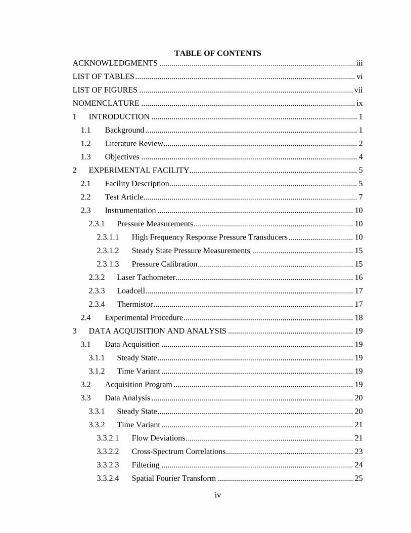
TABLE OF CONTENTS
ACKNOWLEDGMENTS ................................................................................................. iii
LIST OF TABLES ............................................................................................................. vi
LIST OF FIGURES .......................................................................................................... vii
NOMENCLATURE .......................................................................................................... ix
1 INTRODUCTION ...................................................................................................... 1
1.1 Background ......................................................................................................... 1
1.2 Literature Review................................................................................................ 2
1.3 Objectives ........................................................................................................... 4
2 EXPERIMENTAL FACILITY ................................................................................... 5
2.1 Facility Description ............................................................................................. 5
2.2 Test Article.......................................................................................................... 7
2.3 Instrumentation ................................................................................................. 10
2.3.1 Pressure Measurements ............................................................................... 10
2.3.1.1 High Frequency Response Pressure Transducers ................................ 10
2.3.1.2 Steady State Pressure Measurements .................................................. 15
2.3.1.3 Pressure Calibration ............................................................................. 15
2.3.2 Laser Tachometer........................................................................................ 16
2.3.3 Loadcell....................................................................................................... 17
2.3.4 Thermistor ................................................................................................... 17
2.4 Experimental Procedure .................................................................................... 18
3 DATA ACQUISITION AND ANALYSIS .............................................................. 19
3.1 Data Acquisition ............................................................................................... 19
3.1.1 Steady State ................................................................................................. 19
3.1.2 Time Variant ............................................................................................... 19
3.2 Acquisition Program ......................................................................................... 19
3.3 Data Analysis .................................................................................................... 20
3.3.1 Steady State ................................................................................................. 20
3.3.2 Time Variant ............................................................................................... 21
3.3.2.1 Flow Deviations ................................................................................... 21
3.3.2.2 Cross-Spectrum Correlations ............................................................... 23
3.3.2.3 Filtering ............................................................................................... 24
3.3.2.4 Spatial Fourier Transform ................................................................... 25
v
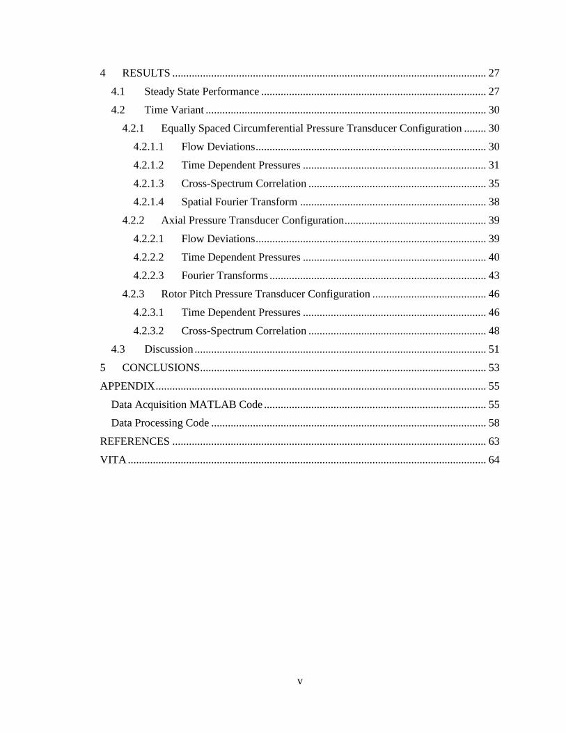
4 RESULTS ................................................................................................................. 27
4.1 Steady State Performance ................................................................................. 27
4.2 Time Variant ..................................................................................................... 30
4.2.1 Equally Spaced Circumferential Pressure Transducer Configuration ........ 30
4.2.1.1 Flow Deviations ................................................................................... 30
4.2.1.2 Time Dependent Pressures .................................................................. 31
4.2.1.3 Cross-Spectrum Correlation ................................................................ 35
4.2.1.4 Spatial Fourier Transform ................................................................... 38
4.2.2 Axial Pressure Transducer Configuration ................................................... 39
4.2.2.1 Flow Deviations ................................................................................... 39
4.2.2.2 Time Dependent Pressures .................................................................. 40
4.2.2.3 Fourier Transforms .............................................................................. 43
4.2.3 Rotor Pitch Pressure Transducer Configuration ......................................... 46
4.2.3.1 Time Dependent Pressures .................................................................. 46
4.2.3.2 Cross-Spectrum Correlation ................................................................ 48
4.3 Discussion ......................................................................................................... 51
5 CONCLUSIONS....................................................................................................... 53
APPENDIX ....................................................................................................................... 55
Data Acquisition MATLAB Code ................................................................................ 55
Data Processing Code ................................................................................................... 58
REFERENCES ................................................................................................................. 63
VITA ................................................................................................................................. 64

vi
LIST OF TABLES
Table 2-1: Operating conditions at the design point and mid-span properties of the
UKLSRC. Credit: Fleeter et al. (1980) ............................................................................... 8
Table 2-2: Kulite Miniature XT Pressure Transducer Specifications. Credit: Kulite (2014)
........................................................................................................................................... 10
vii
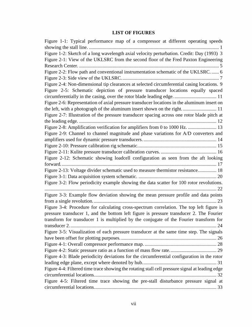
LIST OF FIGURES
Figure 1-1: Typical performance map of a compressor at different operating speeds
showing the stall line. ......................................................................................................... 1
Figure 1-2: Sketch of a long wavelength axial velocity perturbation. Credit: Day (1993) 3
Figure 2-1: View of the UKLSRC from the second floor of the Fred Paxton Engineering
Research Center. ................................................................................................................. 5
Figure 2-2: Flow path and conventional instrumentation schematic of the UKLSRC. ...... 6
Figure 2-3: Side view of the UKLSRC. .............................................................................. 7
Figure 2-4: Non-dimensional tip clearances at selected circumferential casing locations. 9
Figure 2-5: Schematic depiction of pressure transducer locations equally spaced
circumferentially in the casing, over the rotor blade leading edge. .................................. 11
Figure 2-6: Representation of axial pressure transducer locations in the aluminum insert on
the left, with a photograph of the aluminum insert shown on the right. ........................... 11
Figure 2-7: Illustration of the pressure transducer spacing across one rotor blade pitch at
the leading edge. ............................................................................................................... 12
Figure 2-8: Amplification verification for amplifiers from 0 to 1000 Hz. ....................... 13
Figure 2-9: Channel to channel magnitude and phase variations for A/D converters and
amplifiers used for dynamic pressure transducers. ........................................................... 14
Figure 2-10: Pressure calibration rig schematic................................................................ 15
Figure 2-11: Kulite pressure transducer calibration curves. ............................................. 16
Figure 2-12: Schematic showing loadcell configuration as seen from the aft looking
forward. ............................................................................................................................. 17
Figure 2-13: Voltage divider schematic used to measure thermistor resistance. .............. 18
Figure 3-1: Data acquisition system schematic. ............................................................... 20
Figure 3-2: Flow periodicity example showing the data scatter for 100 rotor revolutions.
........................................................................................................................................... 22
Figure 3-3: Example flow deviation showing the mean pressure profile and data points
from a single revolution. ................................................................................................... 23
Figure 3-4: Procedure for calculating cross-spectrum correlation. The top left figure is
pressure transducer 1, and the bottom left figure is pressure transducer 2. The Fourier
transform for transducer 1 is multiplied by the conjugate of the Fourier transform for
transducer 2. ...................................................................................................................... 24
Figure 3-5: Visualization of each pressure transducer at the same time step. The signals
have been offset for plotting purposes. ............................................................................. 26
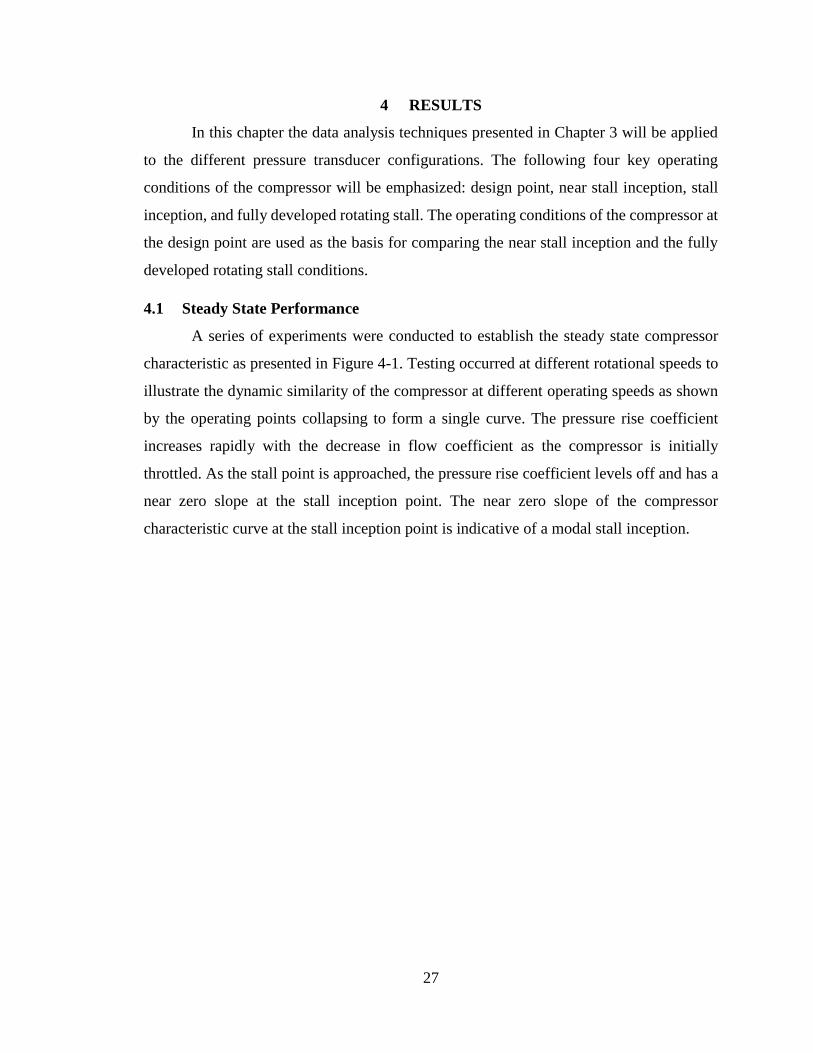
Figure 4-1: Overall compressor performance map. .......................................................... 28
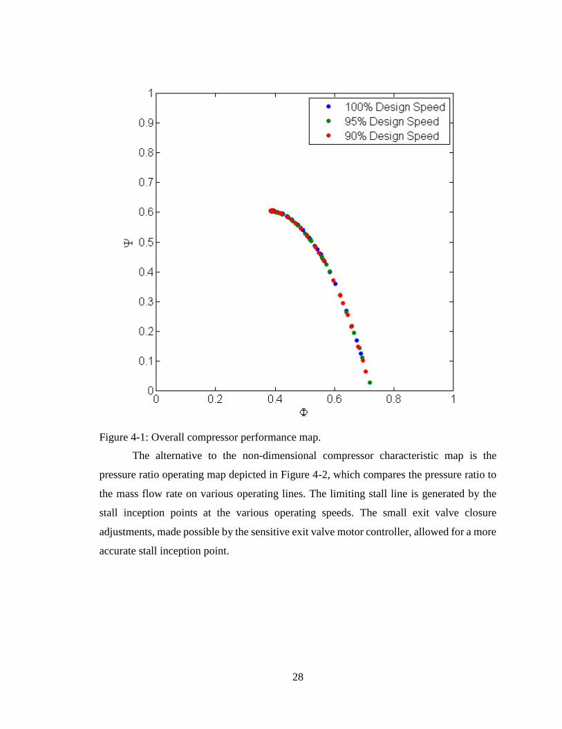
Figure 4-2: Static pressure ratio as a function of mass flow rate. ..................................... 29
Figure 4-3: Blade periodicity deviations for the circumferential configuration in the rotor
leading edge plane, except where denoted by hub. ........................................................... 31
Figure 4-4: Filtered time trace showing the rotating stall cell pressure signal at leading edge
circumferential locations. .................................................................................................. 32
Figure 4-5: Filtered time trace showing the pre-stall disturbance pressure signal at
circumferential locations. .................................................................................................. 33
viii
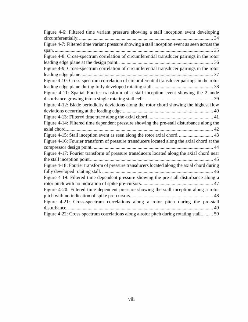
Figure 4-6: Filtered time variant pressure showing a stall inception event developing
circumferentially. .............................................................................................................. 34
Figure 4-7: Filtered time variant pressure showing a stall inception event as seen across the
span. .................................................................................................................................. 35
Figure 4-8: Cross-spectrum correlation of circumferential transducer pairings in the rotor
leading edge plane at the design point. ............................................................................. 36
Figure 4-9: Cross-spectrum correlation of circumferential transducer pairings in the rotor
leading edge plane............................................................................................................. 37
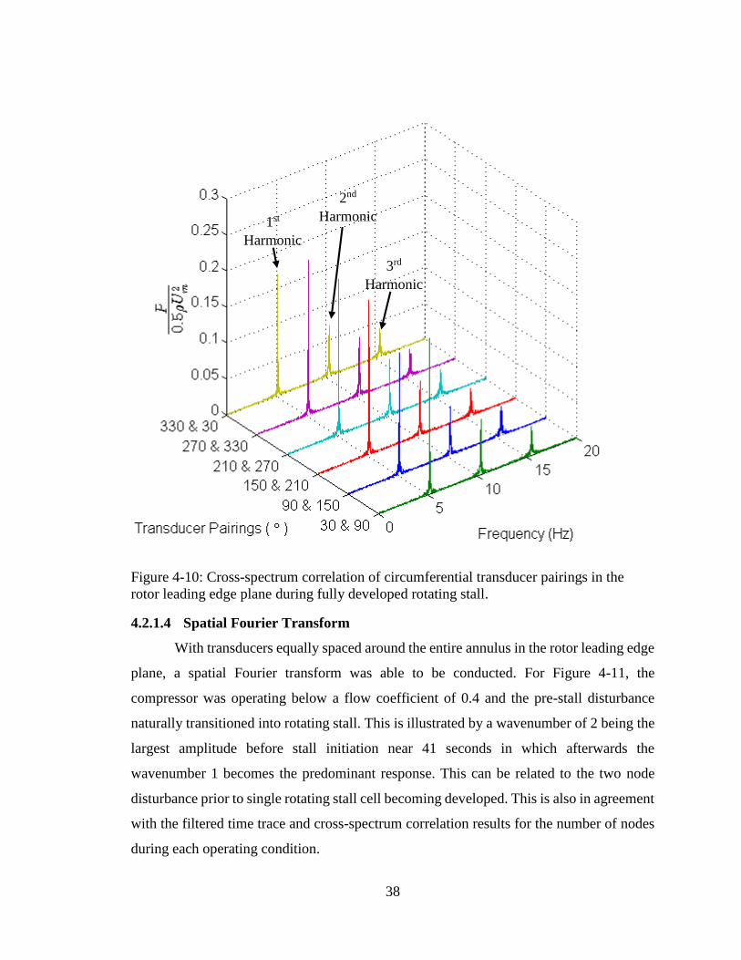
Figure 4-10: Cross-spectrum correlation of circumferential transducer pairings in the rotor
leading edge plane during fully developed rotating stall. ................................................. 38
Figure 4-11: Spatial Fourier transform of a stall inception event showing the 2 node
disturbance growing into a single rotating stall cell. ........................................................ 39
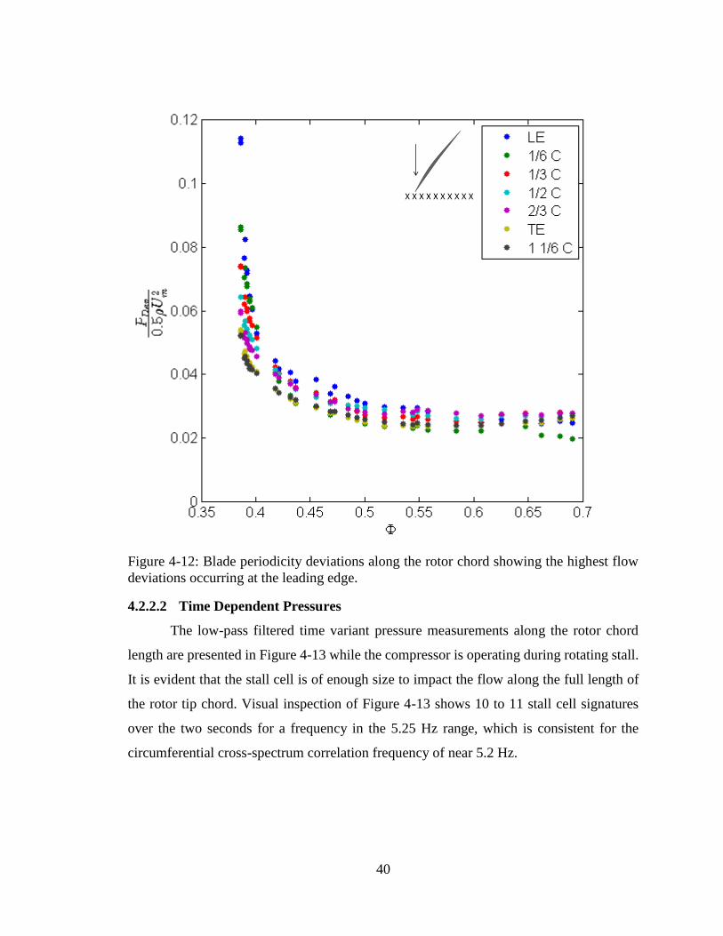
Figure 4-12: Blade periodicity deviations along the rotor chord showing the highest flow
deviations occurring at the leading edge. .......................................................................... 40
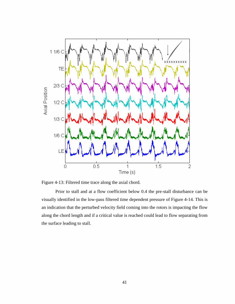
Figure 4-13: Filtered time trace along the axial chord. ..................................................... 41
Figure 4-14: Filtered time dependent pressure showing the pre-stall disturbance along the
axial chord. ........................................................................................................................ 42
Figure 4-15: Stall inception event as seen along the rotor axial chord. ............................ 43
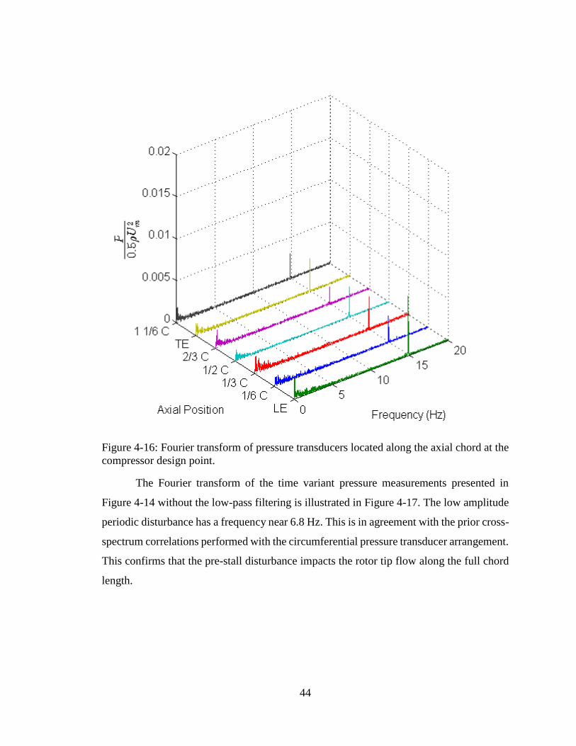
Figure 4-16: Fourier transform of pressure transducers located along the axial chord at the
compressor design point. .................................................................................................. 44
Figure 4-17: Fourier transform of pressure transducers located along the axial chord near
the stall inception point. .................................................................................................... 45
Figure 4-18: Fourier transform of pressure transducers located along the axial chord during
fully developed rotating stall. ........................................................................................... 46
Figure 4-19: Filtered time dependent pressure showing the pre-stall disturbance along a
rotor pitch with no indication of spike pre-cursors. .......................................................... 47
Figure 4-20: Filtered time dependent pressure showing the stall inception along a rotor
pitch with no indication of spike pre-cursors. ................................................................... 48
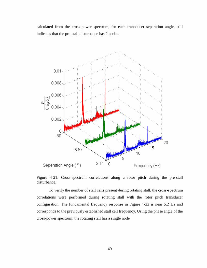
Figure 4-21: Cross-spectrum correlations along a rotor pitch during the pre-stall
disturbance. ....................................................................................................................... 49
Figure 4-22: Cross-spectrum correlations along a rotor pitch during rotating stall. ......... 50

ix
NOMENCLATURE
Greek Symbols
α Speed of sound
θ Transducer spacing
Θ Phase angle
ρ Density
Φ Flow coefficient
Ψ Pressure rise coefficient
Ω Rotational speed
Latin Symbols
Ac Compressor flow through area
B Greitzer parameter
C Chord length
CSC Cross-spectrum correlation
Cx Inlet velocity
F Force
FT Fourier transform
i Data point
k Data points per revolution
L Loadcell lever length
Lc Effective compressor duct length
LC Loadcell
n Number of nodes
N Rotational speed

x
m Number of revolutions
P Pressure
Pexit Exit static pressure
PDev Flow periodicity breakdown
Po Stagnation pressure
PRev Revolution pressure response
PRev̅̅ ̅̅ ̅ Averaged revolution pressure response
P01 Atmospheric pressure
Rres Resistor resistance
Rtherm Thermistor resistance
SRev Standard deviation for revolution pressure response
T Temperature
To Stagnation temperature
Um Mean blade speed
V Plenum volume
Ve Excitation voltage
Vo Output voltage
1
1 INTRODUCTION
1.1 Background
The necessity to understand the fundamental problems associated with the design
and operation of turbomachines becomes increasingly important as engineers strive to
enhance turbomachinery performance. One of the challenges encountered in the design and
operation of compressors for both commercial and military aircraft gas turbine engines is
compressor stall. Not only does stall limit the operating range of compressors, but it will
also induce large cyclic stresses that can lead to fatigue failures during operation.
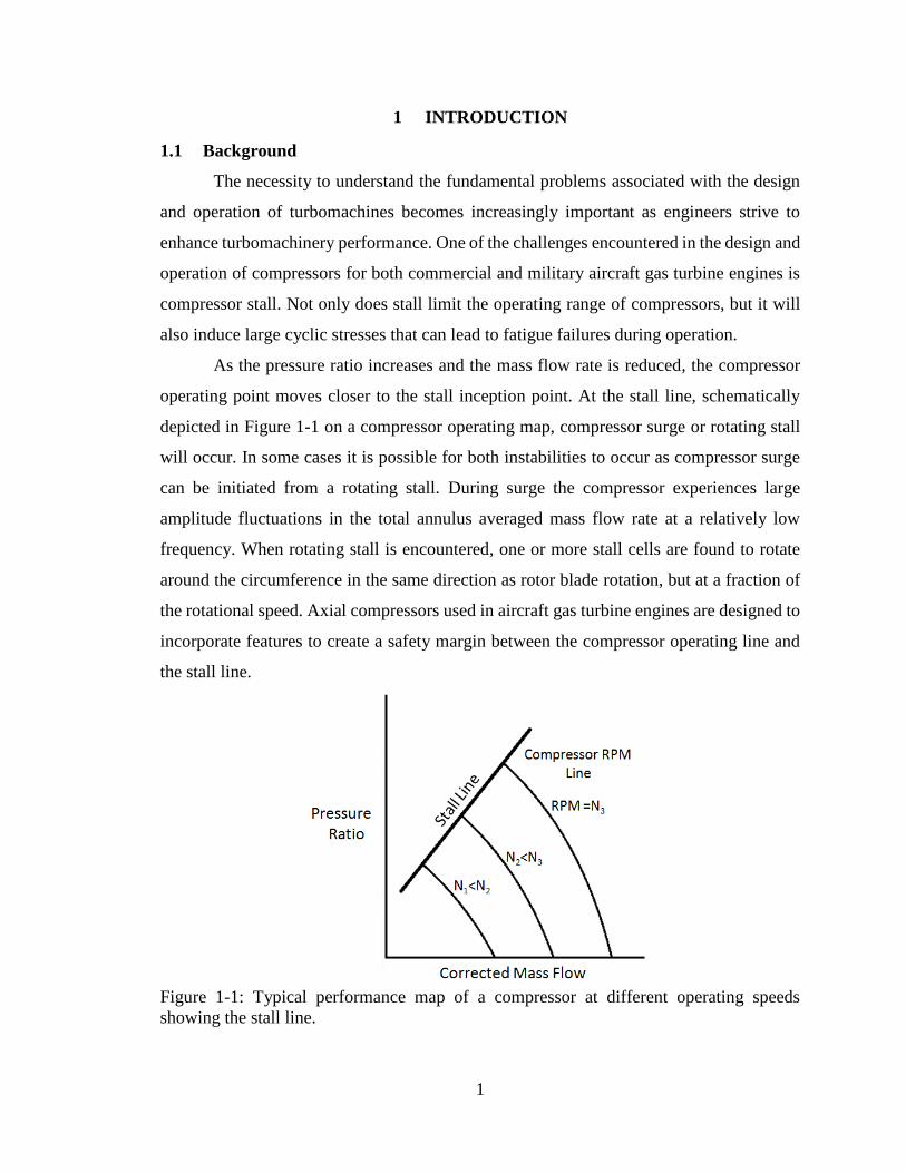
As the pressure ratio increases and the mass flow rate is reduced, the compressor
operating point moves closer to the stall inception point. At the stall line, schematically
depicted in Figure 1-1 on a compressor operating map, compressor surge or rotating stall
will occur. In some cases it is possible for both instabilities to occur as compressor surge
can be initiated from a rotating stall. During surge the compressor experiences large
amplitude fluctuations in the total annulus averaged mass flow rate at a relatively low
frequency. When rotating stall is encountered, one or more stall cells are found to rotate
around the circumference in the same direction as rotor blade rotation, but at a fraction of
the rotational speed. Axial compressors used in aircraft gas turbine engines are designed to
incorporate features to create a safety margin between the compressor operating line and
the stall line.
Figure 1-1: Typical performance map of a compressor at different operating speeds
showing the stall line.
2
1.2 Literature Review
The development of analyses to understand and predict stall is an area of research
interest. Due to the complexity of the flow field, including flow separation, and limitations
in turbulence modeling, accurate prediction of stall has remained elusive. The literature in
this area is voluminous and the following literature review focuses on papers that are
directly related to the presented work.
The aerodynamic instability of surge was characterized by Greitzer (1981) with a
relationship known as the Greitzer-B parameter as seen in Equation 1-1. Greitzer theorized
that the stability of a pumping system could be determined through the use of rotor speed,
speed of sound, plenum volume, compressor flow through area, and an effective length of
the compressor duct. It was found that there is a critical value of B which determined
whether the type of compressor instability experienced would be surge or rotating stall.
Stenning (1980) demonstrated that in high pressure ratio compressors surge may be
triggered very rapidly by a rotating stall and that the dip in the pressure rise caused by the
rotating stall may be sufficient to induce surge. For low pressure ratio machines, like the
University of Kentucky Low Speed Research Compressor (UKLSRC), Stenning showed
that the compressors may not surge at all. The calculated Greitzer-B parameter value for
the UKLSRC is estimated to be 0.08, which is well below the critical value for surge. The
UKLSRC has been experimentally proven not to experience surge.
𝐵 =𝑈
2𝛼√
𝑉
𝐴𝑐𝐿𝑐 (1-1)
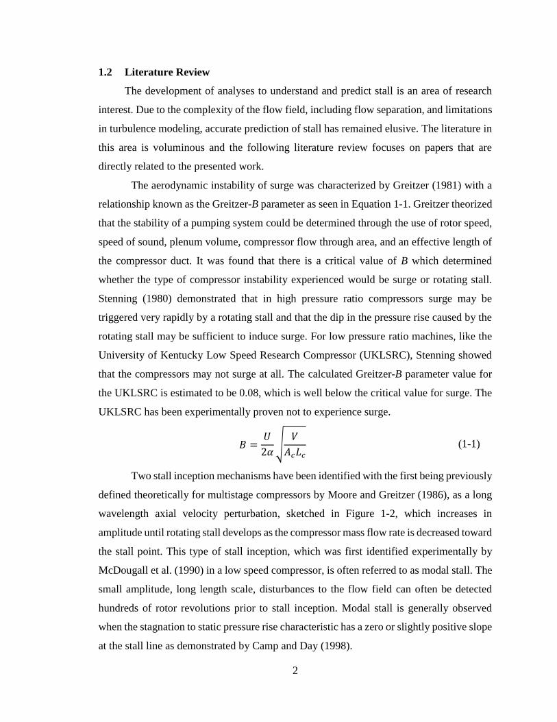
Two stall inception mechanisms have been identified with the first being previously
defined theoretically for multistage compressors by Moore and Greitzer (1986), as a long
wavelength axial velocity perturbation, sketched in Figure 1-2, which increases in
amplitude until rotating stall develops as the compressor mass flow rate is decreased toward
the stall point. This type of stall inception, which was first identified experimentally by
McDougall et al. (1990) in a low speed compressor, is often referred to as modal stall. The
small amplitude, long length scale, disturbances to the flow field can often be detected
hundreds of rotor revolutions prior to stall inception. Modal stall is generally observed
when the stagnation to static pressure rise characteristic has a zero or slightly positive slope
at the stall line as demonstrated by Camp and Day (1998).
3
Figure 1-2: Sketch of a long wavelength axial velocity perturbation. Credit: Day (1993)
The second stall inception mechanism is a short wavelength disturbance, typically
smaller than a few blade passages in size, which can be generated through a local flow
separation that appears to be restricted to the tip region as shown by Day (1993). This stall
inception gets the name ‘spike’ because any pressure measurement taken upstream of a
developing disturbance will show an upward spike while velocity measurements will show
a downward spike. Spike stall is found in compressors that feature a negative slope in the
stagnation to static pressure rise characteristic at the stall line.
Recent research has also focused on resolving the breakdown of flow periodicity as
stall is approached. Blade periodicity is how repeatable the blade passage response is from
one revolution to the next and gives an indication to the amount of breakdown in the flow
passage. An investigation by Young et al. (2011), while using a single stage low speed
compressor, found an increase in the irregularity in the blade passage distribution as the
compressor was throttled to stall. In the same investigation it was shown that the rotor tip
clearance levels and eccentricity play a factor into the amount of unsteadiness and can
greatly impact the flow coefficient for which a compressor stalls. Compressor eccentricity
is quoted as the percentage of the average tip clearance size, an eccentricity of 200% would
lead to blades rubbing the casing during operation at one circumferential location. For an
eccentric compressor the area of minimum clearance is expected to be more stable than the
area with the largest clearance. The tip clearances of the UKLSRC are smaller and more
uniform than those studied by Young et al (2011).

4
1.3 Objectives
In this investigation, instrumentation, data acquisition, and data analysis procedures
were established and used to investigate the stall inception characteristics of the University
of Kentucky Low Speed Research Compressor (UKLSRC). The investigation utilized
casing mounted high frequency response pressure transducers in different geometric
configurations.
The overall objective of this research was to use the instrumentation configurations
and data analysis procedures to investigate stall inception in a low speed axial flow
compressor. The specific objectives were to utilize the detailed measurements of the time-
variant pressure flow field in the rotor casing region to quantify the developmental features
of rotating stall. In doing so, the breakdown of flow periodicity as the flow coefficient is
reduced was investigated along with the development of structured disturbances in the
casing endwall region. This work was directed towards furthering the understanding of
compressor stall inception.
This facility has all of the capabilities necessary to experimentally investigate stall
inception.
5
2 EXPERIMENTAL FACILITY
2.1 Facility Description
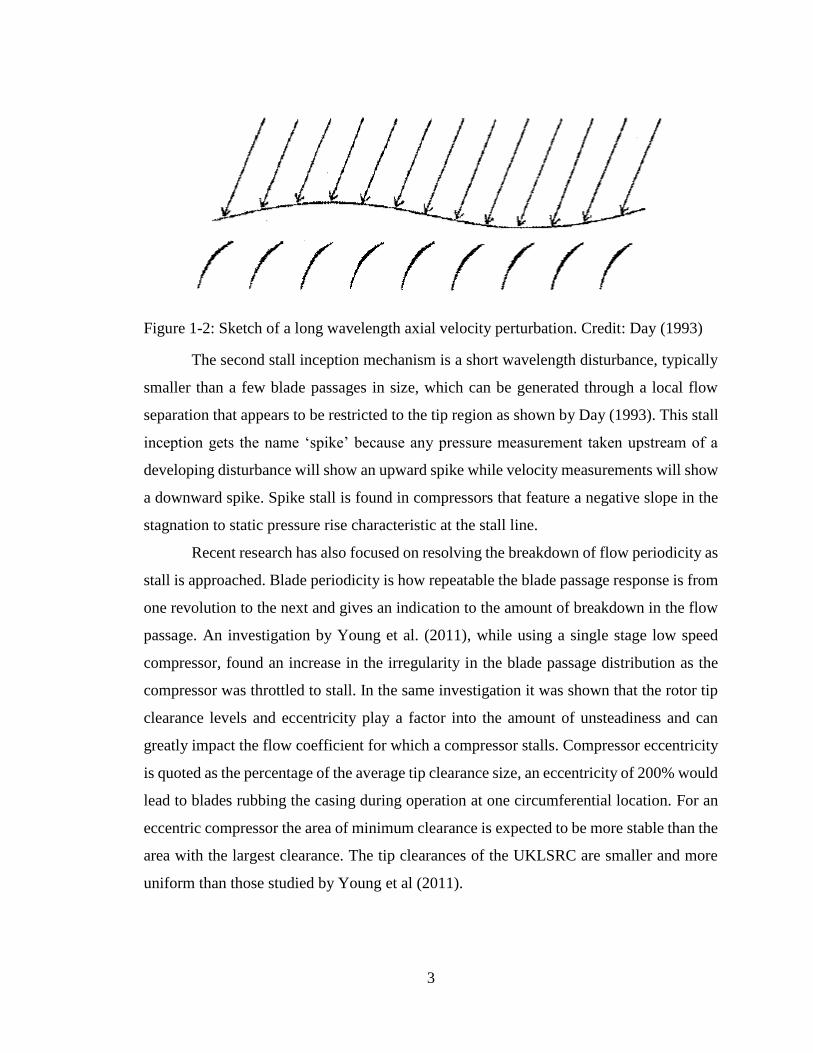
The experimental program was conducted in the Fred Paxton Engineering Research
Center on the campus of West Kentucky Community and Technical College in Paducah,
Kentucky. The building is the home to the University of Kentucky Low Speed Research
Compressor (UKLSRC) as seen from the second floor in Figure 2-1. The facility is capable
of experimentally evaluating the aerodynamic operation of an axial compressor.
Figure 2-1: View of the UKLSRC from the second floor of the Fred Paxton Engineering
Research Center.
The air used by the facility is the ambient room air without any filtration or treatment.
Due to the large ceiling height of the research facility, the compressor is run prior to the
acquisition of data until the temperature of the room has reached equilibrium. A 50
horsepower DC electric motor with tachogenerator feedback is used to provide stable
rotational speeds. The flow exits from the test section radially and the mass flow rate
through the compressor is controlled by a motorized valve in the exit plane which acts as
a throttling valve.
Conventional steady state instrumentation, shown in Figure 2-2, was utilized to
measure the inlet and exit flow fields and to define the compressor operating map. The test
section inlet velocity profile, 2.2 rotor tip chord lengths upstream of the rotor blades, was
determined with six equal circumferentially spaced eleven element total pressure rakes plus
eight hub and casing static pressure taps. The instrumentation capability exists to measure
the rotor exit flow field using a ten-element total pressure rake and a ten-element
6
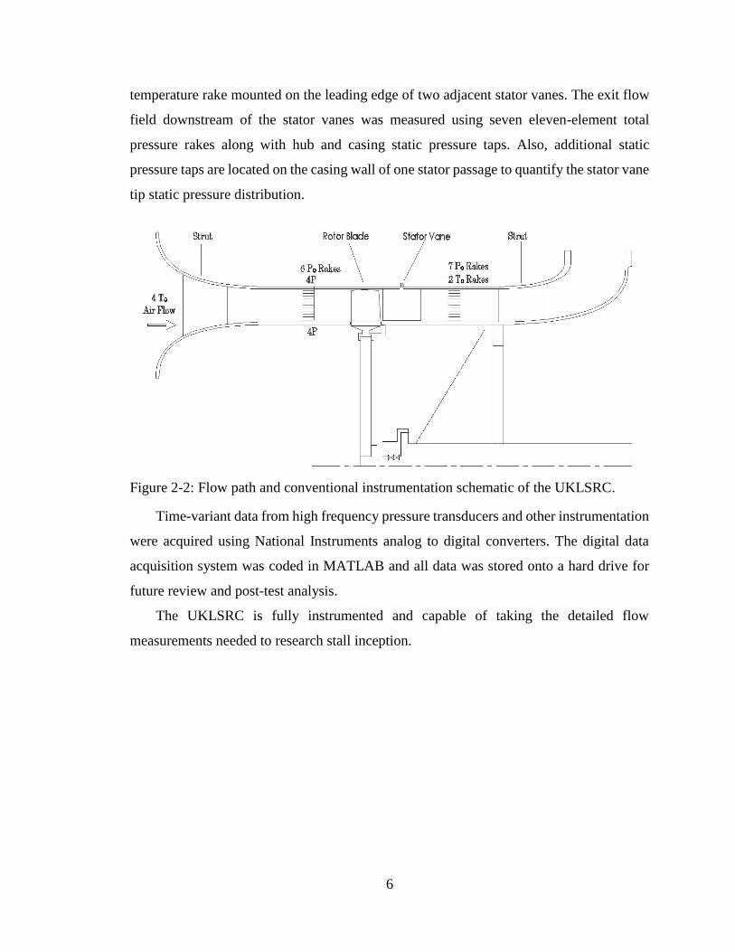
temperature rake mounted on the leading edge of two adjacent stator vanes. The exit flow
field downstream of the stator vanes was measured using seven eleven-element total
pressure rakes along with hub and casing static pressure taps. Also, additional static
pressure taps are located on the casing wall of one stator passage to quantify the stator vane
tip static pressure distribution.
Figure 2-2: Flow path and conventional instrumentation schematic of the UKLSRC.
Time-variant data from high frequency pressure transducers and other instrumentation
were acquired using National Instruments analog to digital converters. The digital data
acquisition system was coded in MATLAB and all data was stored onto a hard drive for
future review and post-test analysis.
The UKLSRC is fully instrumented and capable of taking the detailed flow
measurements needed to research stall inception.

7
2.2 Test Article
In this study the stall inception of UKLSRC is considered, Figure 2-3. The
compressor is a fully instrumented single stage axial flow machine whose design reflects
the loading levels, geometry, and loss levels of the aft stages of a multistage compressor.
The test section has constant tip and hub diameters, with a hub/tip radius ratio of 0.80. The
large size of the compressor, with a casing diameter of 1.22 m, permits large quantities of
instrumentation to be utilized for the quantification of the fundamental flow physics.
Figure 2-3: Side view of the UKLSRC.
The 42 rotor blades and 40 stator vanes have aspect ratios of approximately 1 and
are based upon the NACA 65 series airfoil design. The airfoil mean section characteristics
and compressor design point condition are given in Table 2-1. The rotor and stator airfoil
designs have large camber angles in the hub region. The rotor blades have a maximum
thickness of 7% of the chord at the hub that varies linearly to 4% of chord at the tip. The
rotor blade chord also tapers linearly from hub to tip resulting in a solidity of nearly 1.6 at
the hub and 1.3 at the tip. The stator vane has a constant thickness distribution from hub to
tip with a solidity varying from 1.68 at the hub to 1.35 at the tip. The rotor blades and stator

8
vanes are made of fiberglass material molded around a steel spar that passes through the
airfoil.
Table 2-1: Operating conditions at the design point and mid-span properties of the
UKLSRC. Credit: Fleeter et al. (1980)
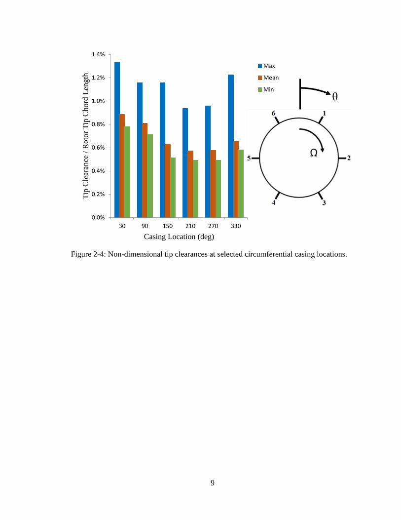
The mean rotor blade tip clearance normalized by the rotor blade tip chord is 0.69%
and when normalized by the annulus height is 0.64%. More detailed statistics of the rotor
blade clearances at selected circumferential locations is illustrated in Figure 2-4. The
statistics were generated by measuring the rotor tip clearance using feeler gauges with an
uncertainty of 0.01 mm along the entire chord length at each designated circumferential
location for each of the rotor blades. The compressor features an eccentricity of 43%.
Rotor Stator
Airfoil Type NACA 65 Series NACA 65 Series
Number of Airfoils 42 40
Chord, c, (cm) 11.40 12.93
Solidity, c/s 1.435 1.516
Camber, Ɵ 20.42° 48.57°
D-factor 0.45 0.41
Aspect Ratio, s/c 1.046 0.943
Mean Blade Speed, Um (m/s) 57
Rotor-Stator Axial Spacing, (cm) 3.772
Flow Rate, (kg/s) 14.07
Design Rotational Speed, RPM 876.3
Number of Stages 1
Design Pressure Ratio 1.0125
Inlet Tip Diameter, (m) 1.22
Hub/Tip Radius Ratio 0.80
Stage Efficiency, (%) 88.1
9
0.0%
0.2%
0.4%
0.6%
0.8%
1.0%
1.2%
1.4%
30 90 150 210 270 330
Tip
Cle
aran
ce /
Roto
r T
ip C
hord
Len
gth
Casing Location (deg)
Max
Mean
Min
Figure 2-4: Non-dimensional tip clearances at selected circumferential casing locations.
10
2.3 Instrumentation
The following section outlines the instrumentation that the UKLSRC has been
outfitted with for performance measurements and stall inception characterization.
2.3.1 Pressure Measurements
The UKLSRC is outfitted to measure dynamic pressures with high frequency
response pressure transducers. The steady state pressures are measured with a digital
pressure scanning array. Details of the pressure measurement instrumentation and
calibration are in the following sub-sections.
2.3.1.1 High Frequency Response Pressure Transducers
High frequency response pressure transducers were used to measure the time
variant pressures occurring within the UKLSRC. Kulite Miniature Ruggedized Pressure
Transducers (XT-190 Series) were chosen to capture the unsteady pressure data; the
specifications are listed in Table 2-2. The transducers were chosen because they are
statically and dynamically capable with a natural frequency exceeding the data acquisition
sampling rate. The transducers are, while being small in size, capable of being flush
mounted to the casing or hub walls.
Table 2-2: Kulite Miniature XT Pressure Transducer Specifications. Credit: Kulite (2014)
Input Pressure Range 35 kPa
Diameter 3.8 mm
Input / Output Impedance 1000 Ohms
Natural Frequency 150 kHz
Acceleration Sensitivity % FS/g Perpendicular 1.5x10⁻³ FS/g
Operating Temperature Range -55°C to 175°C
Weight 4 grams excluding cabling
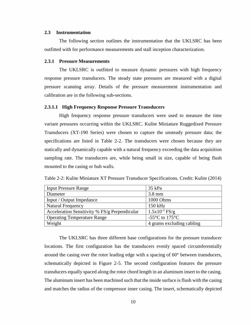
The UKLSRC has three different base configurations for the pressure transducer
locations. The first configuration has the transducers evenly spaced circumferentially
around the casing over the rotor leading edge with a spacing of 60° between transducers,
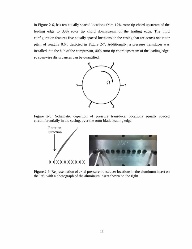
schematically depicted in Figure 2-5. The second configuration features the pressure
transducers equally spaced along the rotor chord length in an aluminum insert to the casing.
The aluminum insert has been machined such that the inside surface is flush with the casing
and matches the radius of the compressor inner casing. The insert, schematically depicted
11
in Figure 2-6, has ten equally spaced locations from 17% rotor tip chord upstream of the
leading edge to 33% rotor tip chord downstream of the trailing edge. The third
configuration features five equally spaced locations on the casing that are across one rotor
pitch of roughly 8.6°, depicted in Figure 2-7. Additionally, a pressure transducer was
installed into the hub of the compressor, 40% rotor tip chord upstream of the leading edge,
so spanwise disturbances can be quantified.
Figure 2-5: Schematic depiction of pressure transducer locations equally spaced
circumferentially in the casing, over the rotor blade leading edge.
Figure 2-6: Representation of axial pressure transducer locations in the aluminum insert on
the left, with a photograph of the aluminum insert shown on the right.
Rotation
Direction

12
Figure 2-7: Illustration of the pressure transducer spacing across one rotor blade pitch at
the leading edge.
The pressure transducers’ outputs are in the low millivolt range so Omega OM5-
WMV amplifiers were used to amplify the signal going into the data acquisition unit. The
amplifiers have a gain of 50 with a quoted output accuracy of 0.08%. The amplification
values were verified using a signal generator to generate a sine wave at various frequencies.
A Fourier Transform was applied to the amplified signal to compare to the pre-amplified
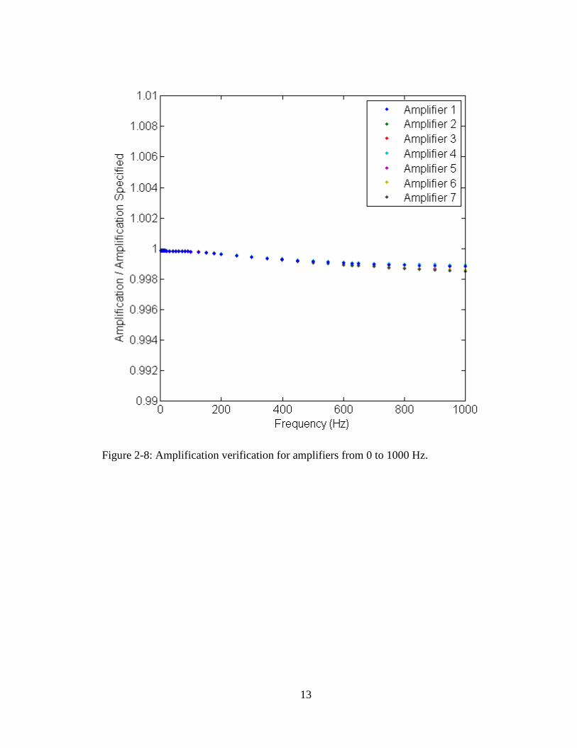
voltages. Figure 2-8 shows a slight trailing in amplitudes past 630 Hz, but it is less than
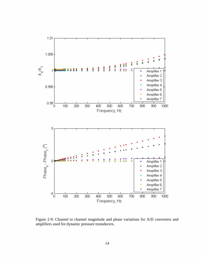
0.2%. Channel to channel comparisons of amplitude ratio and phase angle are shown in
Figure 2-9 for all of the data acquisition channels with amplifiers. For the amplified
channels the phase difference is less than 0.5° under 100 Hz and negligible in the range of
interest.
1 2 3 4 5
13
Figure 2-8: Amplification verification for amplifiers from 0 to 1000 Hz.
14
Figure 2-9: Channel to channel magnitude and phase variations for A/D converters and
amplifiers used for dynamic pressure transducers.
15
2.3.1.2 Steady State Pressure Measurements
For measuring the steady state static and stagnation pressures, a digital pressure
scanning array was used. The digital sensor arrays were manufactured by Scanivalve and
are model DSA3016, which fit inside of the DSAENCL4000 enclosure. Two arrays are
available with the first having a full scale pressure range of 2.5 kPa and the second of 6.9
kPa. Each array has 16 pressure channels for a total of 32. The array features a 16 bit A/D
converter, which has a maximum sampling rate of 625 samples/channel/second, and
communicates with the data acquisition computer with TCP/IP protocol.
2.3.1.3 Pressure Calibration
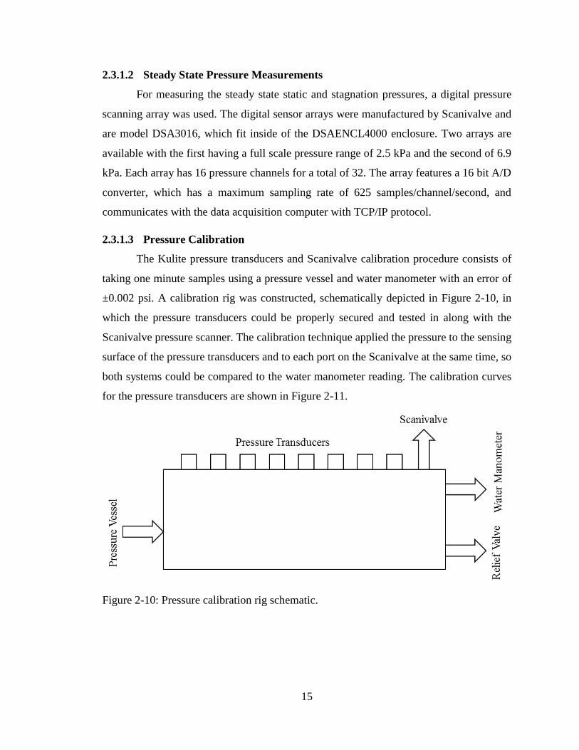
The Kulite pressure transducers and Scanivalve calibration procedure consists of
taking one minute samples using a pressure vessel and water manometer with an error of
±0.002 psi. A calibration rig was constructed, schematically depicted in Figure 2-10, in
which the pressure transducers could be properly secured and tested in along with the
Scanivalve pressure scanner. The calibration technique applied the pressure to the sensing
surface of the pressure transducers and to each port on the Scanivalve at the same time, so
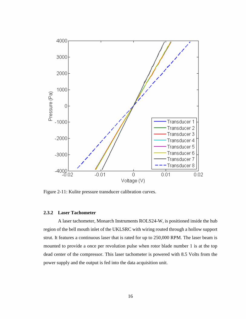
both systems could be compared to the water manometer reading. The calibration curves
for the pressure transducers are shown in Figure 2-11.
Figure 2-10: Pressure calibration rig schematic.
16
Figure 2-11: Kulite pressure transducer calibration curves.
2.3.2 Laser Tachometer
A laser tachometer, Monarch Instruments ROLS24-W, is positioned inside the hub
region of the bell mouth inlet of the UKLSRC with wiring routed through a hollow support
strut. It features a continuous laser that is rated for up to 250,000 RPM. The laser beam is
mounted to provide a once per revolution pulse when rotor blade number 1 is at the top
dead center of the compressor. This laser tachometer is powered with 8.5 Volts from the
power supply and the output is fed into the data acquisition unit.
17
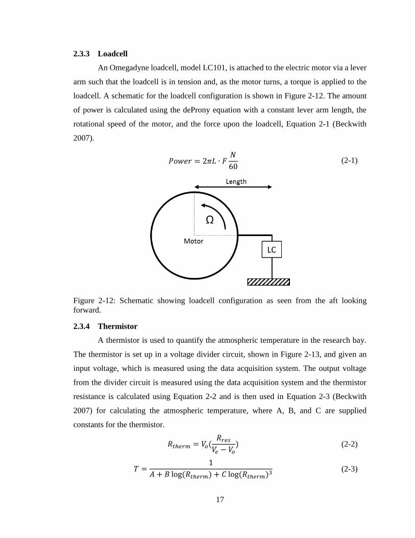
2.3.3 Loadcell
An Omegadyne loadcell, model LC101, is attached to the electric motor via a lever
arm such that the loadcell is in tension and, as the motor turns, a torque is applied to the
loadcell. A schematic for the loadcell configuration is shown in Figure 2-12. The amount
of power is calculated using the deProny equation with a constant lever arm length, the
rotational speed of the motor, and the force upon the loadcell, Equation 2-1 (Beckwith
2007).
Figure 2-12: Schematic showing loadcell configuration as seen from the aft looking
forward.
2.3.4 Thermistor
A thermistor is used to quantify the atmospheric temperature in the research bay.
The thermistor is set up in a voltage divider circuit, shown in Figure 2-13, and given an
input voltage, which is measured using the data acquisition system. The output voltage
from the divider circuit is measured using the data acquisition system and the thermistor
resistance is calculated using Equation 2-2 and is then used in Equation 2-3 (Beckwith
2007) for calculating the atmospheric temperature, where A, B, and C are supplied
constants for the thermistor.
𝑅𝑡ℎ𝑒𝑟𝑚 = 𝑉𝑜(𝑅𝑟𝑒𝑠𝑉𝑒 − 𝑉𝑜
) (2-2)
𝑇 =1
𝐴 + 𝐵 log(𝑅𝑡ℎ𝑒𝑟𝑚) + 𝐶 log(𝑅𝑡ℎ𝑒𝑟𝑚)3 (2-3)
𝑃𝑜𝑤𝑒𝑟 = 2𝜋𝐿 ∙ 𝐹𝑁
60 (2-1)

18
Figure 2-13: Voltage divider schematic used to measure thermistor resistance.
2.4 Experimental Procedure
Unsteady pressure measurements were acquired at discrete operating points up to
the stall inception point and during the transition to rotating stall. For each discrete
operating point, the compressor was given time to settle before data was acquired. Data
was then acquired over a length of time no shorter than 900 rotor revolutions before the
exit valve was moved to change the mass flow rate. In addition, the variable speed throttling
valve was closed at a very slow speed and the unsteady pressure measurements were
continuously recorded transiently as the compressor moves from the design point to fully
developed rotating stall. A linear potentiometer attached to the exit valve quantifies the
displacement of the exit valve from the wide open discharge condition.
19
3 DATA ACQUISITION AND ANALYSIS
3.1 Data Acquisition
Two types of data were acquired, steady state and time variant. The steady state
section details the pressure measurements in the inlet and the exit flow field where the
pressure was assumed to be steady with minimal rotor induced pressure fluctuations and
was sampled at a relatively low sampling frequency. The time variant section details the
measurements that were taken at a high sampling frequency.
For a given operating point the compressor was given time to stabilize from any
transient effects of the exit valve being moved before data was acquired. The steady state
and time variant data were acquired simultaneously. Data was acquired over a minimum
duration of time of 60 seconds, which included 900 or greater rotor revolutions. The exit
valve position was then adjusted and the data acquisition process was repeated.
3.1.1 Steady State
The inlet and exit flow field, static and stagnation pressures, are measured with the
Scanivalve digital pressure scanning array that has an uncertainty of ±0.2% full scale. The
pressures were sampled 250 times per second with the average pressure for each channel
being reported. There were 30 reported values for each pressure channel per data set at a
fixed operating point. The reported values were then averaged to provide a single pressure
value for each of the measurement locations. The Scanivalve digital pressure scanning
array connects to the data acquisition computer using a TCP/IP connection.
3.1.2 Time Variant
The time variant data was digitized using National Instruments A/D modules with
each channel being sampled at 100k samples per second. This sampling rate allows the
high frequency response transducers to acquire detailed measurements of more than 150
points per rotor blade passage at the design rotational speed. The laser tachometer and
loadcell were also sampled at the 100k samples per second sampling rate.
3.2 Acquisition Program
In the early stages of this investigation, the data was being acquired using the
National Instruments LabVIEW program for the time variant data and by manually
querying the steady state pressures from the Scanivalve pressure scanner. The time variant

20
data was being sampled at 50k samples per second, half of the maximum sampling rate,
and at a reduced total number of channels. Data recording and storage issues arose after
acquiring additional instrumentation which lead to the creation of a data acquisition
program using MATLAB.
The data acquisition program was created with the use of the Data Acquisition
Toolbox for MATLAB, and can be found in the Appendix. This allowed for sampling at
the maximum possible rate, providing more points per blade passage, and for Scanivalve
integration using TCP/IP protocols to automatically send commands and retrieve data. The
data acquisition program runs in the background of MATLAB, continuously sampling the
data, and begins writing the data to disk with the push of a button. The hardware
configuration is schematically shown in Figure 3-1 including the data acquisition
computer, pressure scanning system, and amplifiers. The current exit valve position in
terms of percent closed is visible on screen to help in the setting of operating points
allowing for fine adjustments in the near stall region.
Figure 3-1: Data acquisition system schematic.
3.3 Data Analysis
The data analysis techniques used in this study to characterize the flow behavior of
the UKLSRC are detailed in the following section. These techniques could also be applied
to characterize the flow behavior of other turbomachines.
3.3.1 Steady State
The general behavior of any turbomachine can be obtained from dimensional
analysis techniques. Buckingham Π theorem is a method for nondimensionalization by
providing sets of dimensionless parameters from given key variables. A non-dimensional
quantity can be formed, called the flow coefficient, which is calculated by comparing the
K – Pressure transducers
L – Loadcell
O – Laser tachometer
P – Linear potentiometer
T – Temperature
A – Amplifier
NI – National Instruments
SV – Scanivalve
21
axial velocity to the mean blade speed as seen in Equation 3-1 and has a maximum margin
of error of 3.4%. The pressure rise in a low speed compressor can be characterized by using
the non-dimensional pressure rise coefficient. The pressure rise coefficient seen in
Equation 3-2 compares the total static pressure rise to the mean dynamic pressure and has
a maximum margin of error of 2.0%. Comparing the flow coefficient to the pressure rise
coefficient produces a plot of the compressor characteristics. Due to the non-
dimensionality of the parameters all rotational speeds will collapse into a single curve but
Reynolds number effects can become dominate at the stall inception point. The Reynolds
number based off rotor tip chord length at design speed is near 410000 and Reynolds
number effects near stall are small.
3.3.2 Time Variant
The following sub-sections explain the data analysis techniques that were applied
to the time variant pressure measurements.
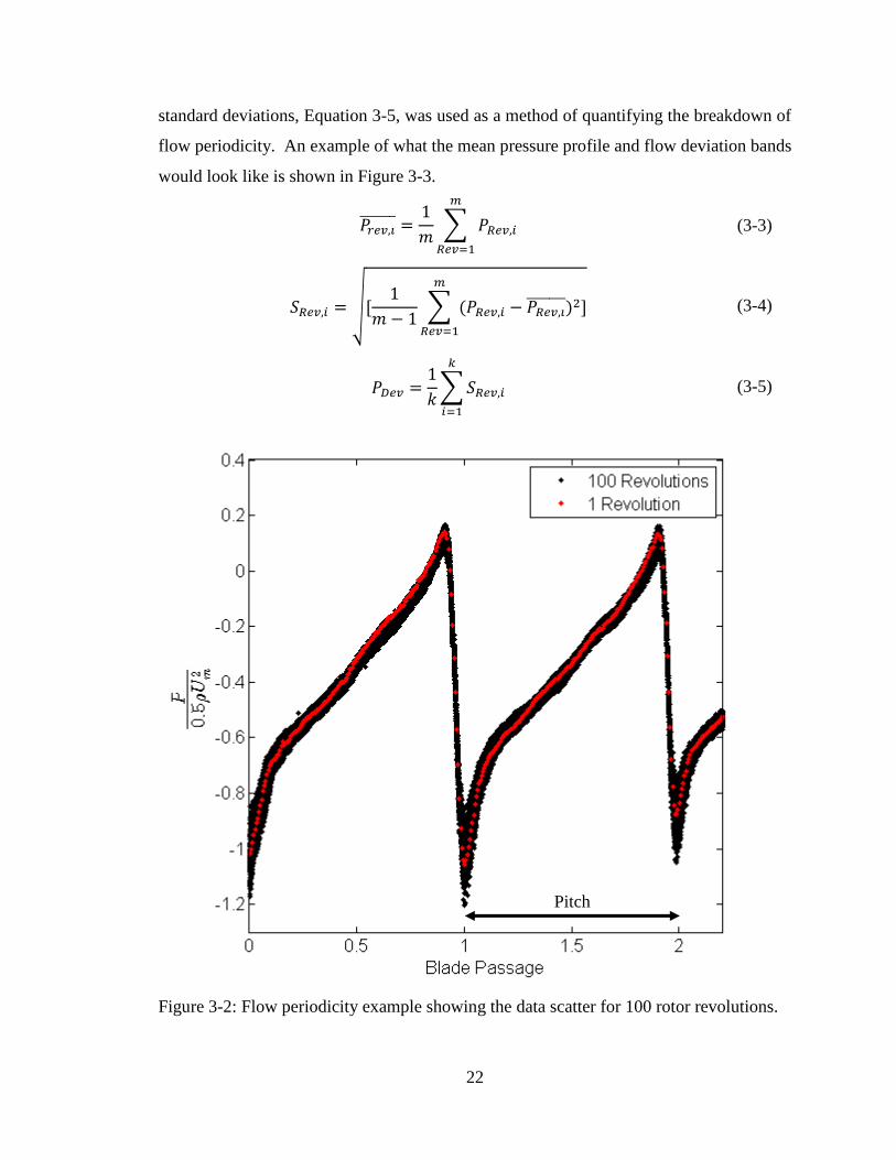
3.3.2.1 Flow Deviations
Flow periodicity is the repeatability of the pressure profile of a rotor passage to be
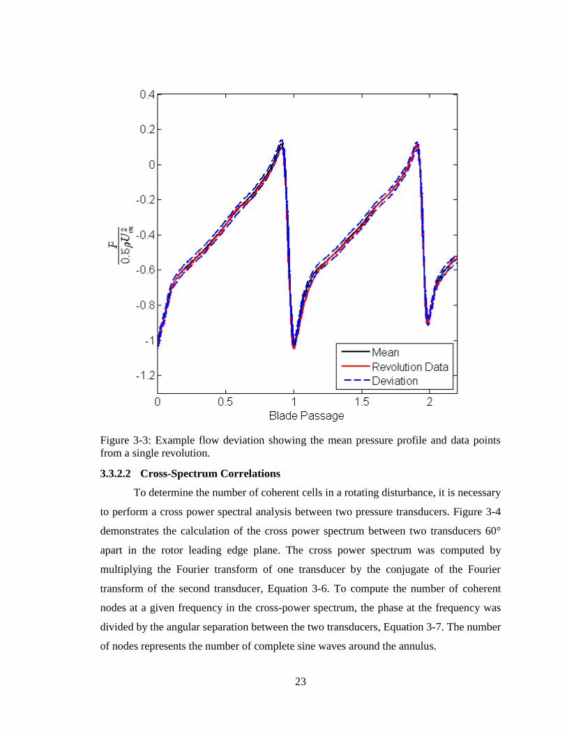
the same between revolutions as illustrated in Figure 3-2 and periodic from passage to
passage. The breakdown of flow periodicity leads to irregularities in the blade passing
signature. The impact of these irregularities can be measured by looking at the standard
deviation of the flow compared to a mean value. The laser tachometer was used as an
indicator of each rotor revolution and was used to split the time domain pressure transducer
signals into a series of revolutions. Each revolution was linearly interpolated to account for
minor differences in the rotational speed. The mean pressure profile was determined by
averaging all of interpolated pressure profiles to achieve a single profile from which the
standard deviation was then calculated for each point across the blade passage through use
of Equation 3-3 and 3-4, respectively. The deviation was calculated for each revolution as
a whole and then for each blade passage between the pressure and suction surfaces, which
does not include the pressure jump over the thickness of the blade. The mean of the
Φ =𝐶𝑥𝑈𝑚
(3-1)
Ψ =𝑃𝑒𝑥𝑖𝑡 − 𝑃0112𝜌𝑈𝑚
2 (3-2)
22
standard deviations, Equation 3-5, was used as a method of quantifying the breakdown of
flow periodicity. An example of what the mean pressure profile and flow deviation bands
would look like is shown in Figure 3-3.
𝑃𝑟𝑒𝑣,𝑖̅̅ ̅̅ ̅̅ =1
𝑚∑ 𝑃𝑅𝑒𝑣,𝑖
𝑚
𝑅𝑒𝑣=1
(3-3)
𝑆𝑅𝑒𝑣,𝑖 = √[1
𝑚 − 1∑ (𝑃𝑅𝑒𝑣,𝑖 − 𝑃𝑅𝑒𝑣,𝑖̅̅ ̅̅ ̅̅ ̅)2𝑚
𝑅𝑒𝑣=1
] (3-4)
𝑃𝐷𝑒𝑣 =1
𝑘∑𝑆𝑅𝑒𝑣,𝑖
𝑘
𝑖=1
(3-5)
Figure 3-2: Flow periodicity example showing the data scatter for 100 rotor revolutions.
Pitch
23
Figure 3-3: Example flow deviation showing the mean pressure profile and data points
from a single revolution.
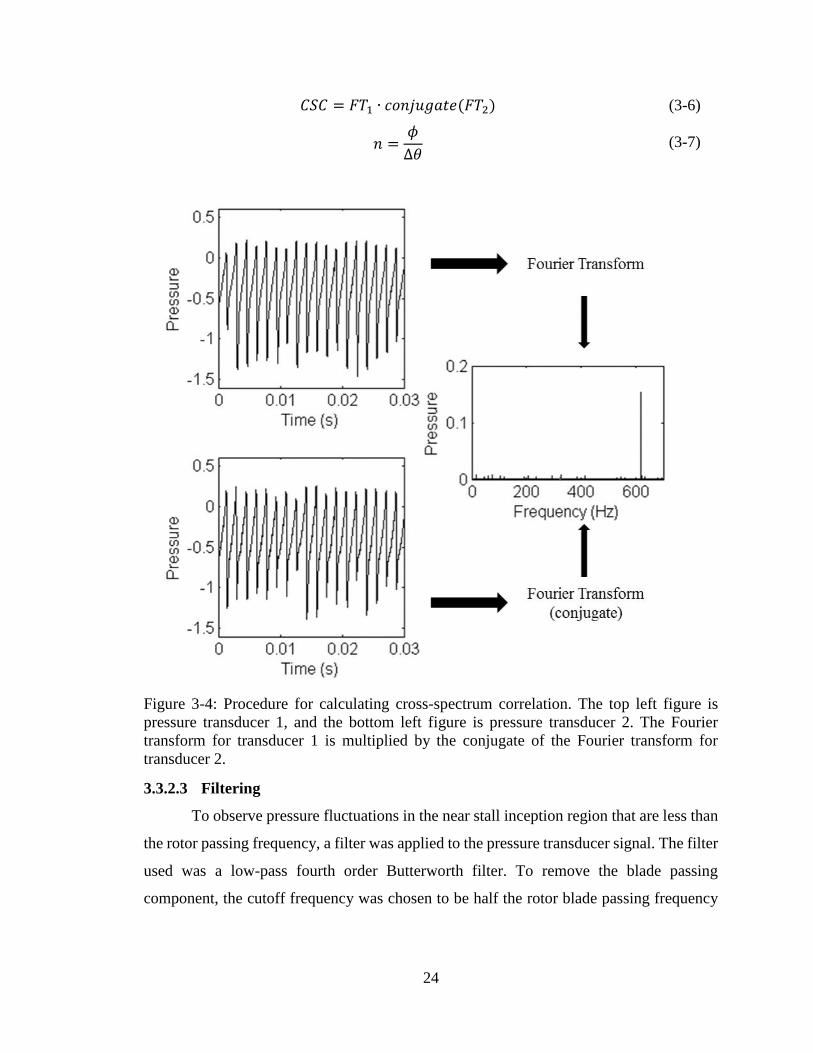
3.3.2.2 Cross-Spectrum Correlations
To determine the number of coherent cells in a rotating disturbance, it is necessary
to perform a cross power spectral analysis between two pressure transducers. Figure 3-4
demonstrates the calculation of the cross power spectrum between two transducers 60°
apart in the rotor leading edge plane. The cross power spectrum was computed by
multiplying the Fourier transform of one transducer by the conjugate of the Fourier
transform of the second transducer, Equation 3-6. To compute the number of coherent
nodes at a given frequency in the cross-power spectrum, the phase at the frequency was
divided by the angular separation between the two transducers, Equation 3-7. The number
of nodes represents the number of complete sine waves around the annulus.
24
𝐶𝑆𝐶 = 𝐹𝑇1 ∙ 𝑐𝑜𝑛𝑗𝑢𝑔𝑎𝑡𝑒(𝐹𝑇2) (3-6)
𝑛 =𝜙
Δ𝜃 (3-7)
Figure 3-4: Procedure for calculating cross-spectrum correlation. The top left figure is
pressure transducer 1, and the bottom left figure is pressure transducer 2. The Fourier
transform for transducer 1 is multiplied by the conjugate of the Fourier transform for
transducer 2.
3.3.2.3 Filtering
To observe pressure fluctuations in the near stall inception region that are less than
the rotor passing frequency, a filter was applied to the pressure transducer signal. The filter
used was a low-pass fourth order Butterworth filter. To remove the blade passing
component, the cutoff frequency was chosen to be half the rotor blade passing frequency
25
with a typical value of 315 Hz. Lower cutoff frequencies were used depending upon
application.
3.3.2.4 Spatial Fourier Transform
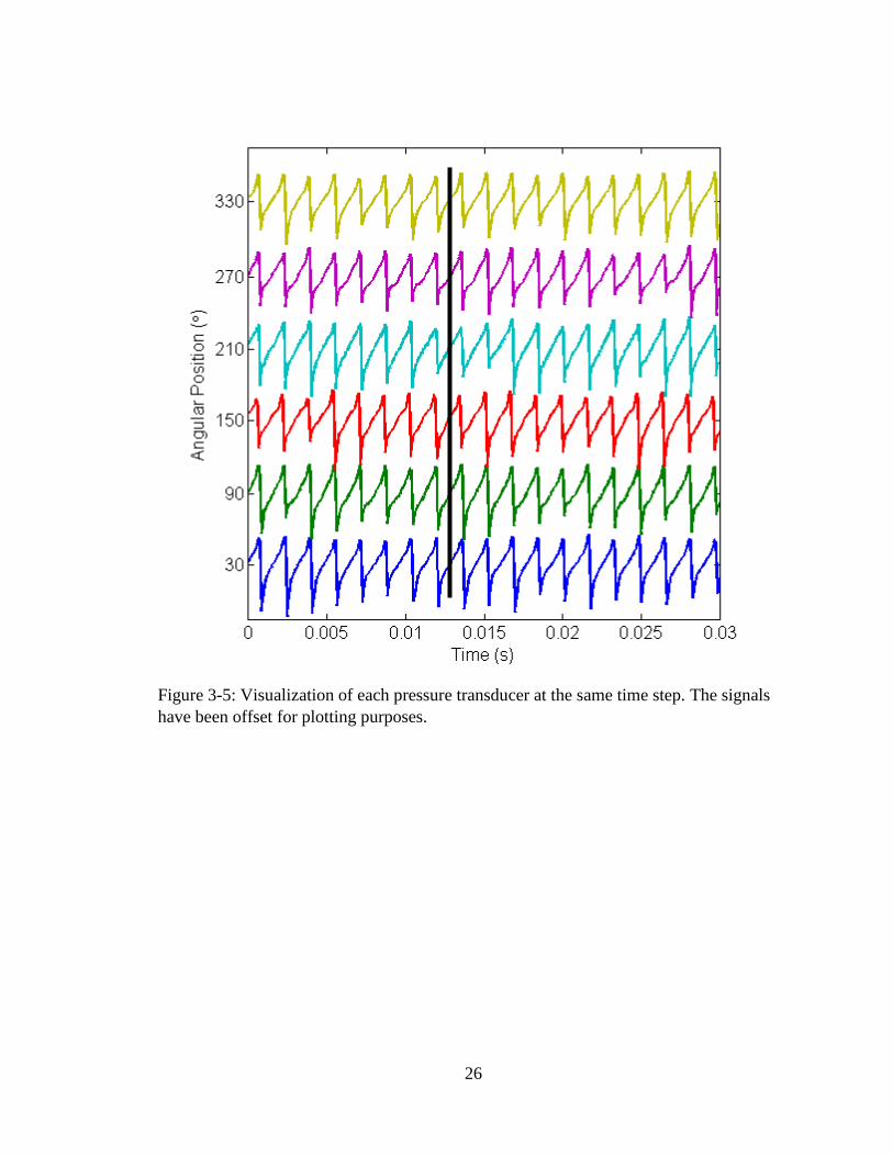
To better understand the stall inception phase, the circumferential array of 6 equally
space pressure transducers in the rotor leading edge plane was used. This method meets
the requirements of capturing the time variant pressure field around the rotor at each instant
in time. The circumferential pressure field was analyzed at each time step shown in Figure
3-5. The compressor has 42 rotor blades, which means 84 pressure transducers are required
to avoid aliasing of the first 42 spatial waves. For this study, only 6 pressure transducers
were available, meaning that aliasing will occur for any wavenumber greater than 3. A low-
pass filter with a cutoff frequency of 9 Hz was used to condition the data due to the spatial
limitations.
26
Figure 3-5: Visualization of each pressure transducer at the same time step. The signals
have been offset for plotting purposes.
27
4 RESULTS
In this chapter the data analysis techniques presented in Chapter 3 will be applied
to the different pressure transducer configurations. The following four key operating
conditions of the compressor will be emphasized: design point, near stall inception, stall
inception, and fully developed rotating stall. The operating conditions of the compressor at
the design point are used as the basis for comparing the near stall inception and the fully
developed rotating stall conditions.
4.1 Steady State Performance
A series of experiments were conducted to establish the steady state compressor
characteristic as presented in Figure 4-1. Testing occurred at different rotational speeds to
illustrate the dynamic similarity of the compressor at different operating speeds as shown
by the operating points collapsing to form a single curve. The pressure rise coefficient
increases rapidly with the decrease in flow coefficient as the compressor is initially
throttled. As the stall point is approached, the pressure rise coefficient levels off and has a
near zero slope at the stall inception point. The near zero slope of the compressor
characteristic curve at the stall inception point is indicative of a modal stall inception.
28
Figure 4-1: Overall compressor performance map.
The alternative to the non-dimensional compressor characteristic map is the
pressure ratio operating map depicted in Figure 4-2, which compares the pressure ratio to
the mass flow rate on various operating lines. The limiting stall line is generated by the
stall inception points at the various operating speeds. The small exit valve closure
adjustments, made possible by the sensitive exit valve motor controller, allowed for a more
accurate stall inception point.
29
Figure 4-2: Static pressure ratio as a function of mass flow rate.
30
4.2 Time Variant
Results will now be presented that used the high frequency response pressure
transducers to track the time variant pressures occurring inside of the compressor. The flow
deviation measurements that track the amount of flow irregularity in the blade periodicity,
Fourier analysis, and time traces will be presented using different pressure transducer
configurations.
4.2.1 Equally Spaced Circumferential Pressure Transducer Configuration
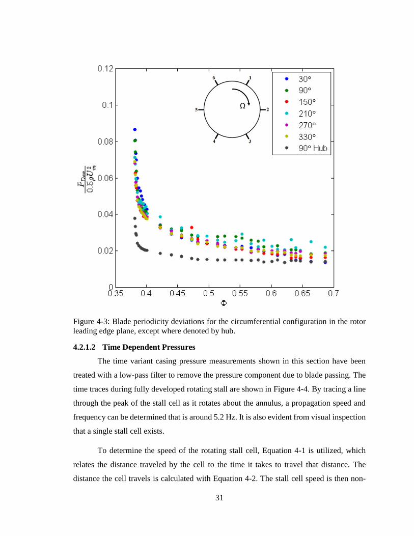
4.2.1.1 Flow Deviations
The flow deviations for transducers in the circumferential configuration are
illustrated in Figure 4-3. As the flow coefficient was decreased, the amount of irregularity
in the blade periodicity increased in a monotonic fashion up to a flow coefficient of
approximately 0.4. Additional throttling of the compressor induced a rotating disturbance
that can be seen by the sharp increase in the irregularity of the flow prior to stall inception.
The distribution of flow irregularities in the rotor leading edge plane was fairly uniform
with no location experiencing a much larger amount than any other. When the pressure
transducer located in the hub of the compressor is considered, the amount of change in flow
irregularities was rather constant until the 0.4 flow coefficient region, in which a large
increase was seen. The overall amplitude of the flow periodicity breakdown was less at the
hub of the compressor due to being away from the tip clearance flow and 40% rotor cord
upstream of the rotor leading edge.
31
Figure 4-3: Blade periodicity deviations for the circumferential configuration in the rotor
leading edge plane, except where denoted by hub.
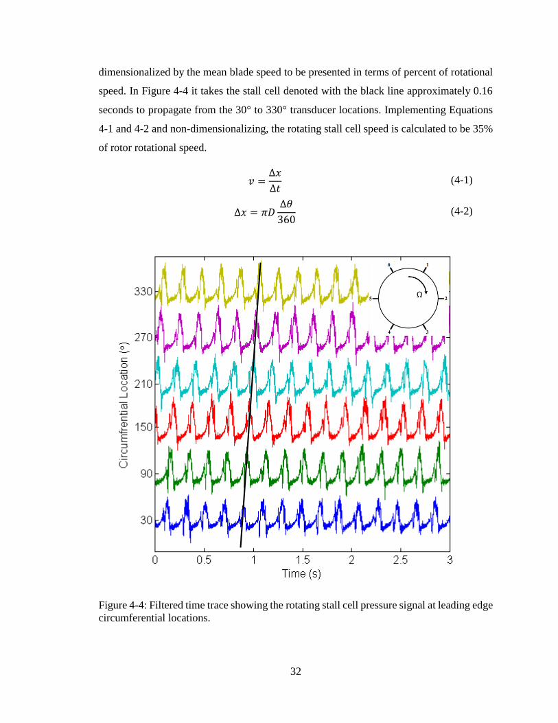
4.2.1.2 Time Dependent Pressures
The time variant casing pressure measurements shown in this section have been
treated with a low-pass filter to remove the pressure component due to blade passing. The
time traces during fully developed rotating stall are shown in Figure 4-4. By tracing a line
through the peak of the stall cell as it rotates about the annulus, a propagation speed and
frequency can be determined that is around 5.2 Hz. It is also evident from visual inspection
that a single stall cell exists.
To determine the speed of the rotating stall cell, Equation 4-1 is utilized, which
relates the distance traveled by the cell to the time it takes to travel that distance. The
distance the cell travels is calculated with Equation 4-2. The stall cell speed is then non-
32
dimensionalized by the mean blade speed to be presented in terms of percent of rotational
speed. In Figure 4-4 it takes the stall cell denoted with the black line approximately 0.16
seconds to propagate from the 30° to 330° transducer locations. Implementing Equations
4-1 and 4-2 and non-dimensionalizing, the rotating stall cell speed is calculated to be 35%
of rotor rotational speed.
𝑣 =∆𝑥
∆𝑡 (4-1)
∆𝑥 = 𝜋𝐷∆𝜃
360 (4-2)
Figure 4-4: Filtered time trace showing the rotating stall cell pressure signal at leading edge
circumferential locations.
33
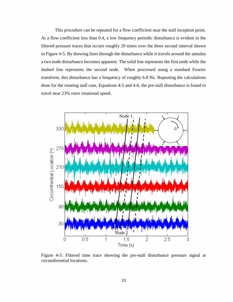
This procedure can be repeated for a flow coefficient near the stall inception point.
At a flow coefficient less than 0.4, a low frequency periodic disturbance is evident in the
filtered pressure traces that occurs roughly 20 times over the three second interval shown
in Figure 4-5. By drawing lines through the disturbance while it travels around the annulus
a two node disturbance becomes apparent. The solid line represents the first node while the
dashed line represents the second node. When processed using a standard Fourier
transform, this disturbance has a frequency of roughly 6.8 Hz. Repeating the calculations
done for the rotating stall case, Equations 4-5 and 4-6, the pre-stall disturbance is found to
travel near 23% rotor rotational speed.
Figure 4-5: Filtered time trace showing the pre-stall disturbance pressure signal at
circumferential locations.
Node 1
Node 2

34
This periodic pre-stall disturbance will eventually reach a critical condition and
stall will be initiated in the compressor. A stall inception event can be seen in Figure 4-6,
which shows the pre-stall disturbance at 0 seconds with the stall initiation occurring near
1.5 seconds and the mature stall cell being seen before the 3 second mark. The stall cell
rapidly grows from the inception event that occurs at about 1.5 seconds at the 210°
transducer location into a fully developed rotating stall cell.
Figure 4-6: Filtered time variant pressure showing a stall inception event developing
circumferentially.
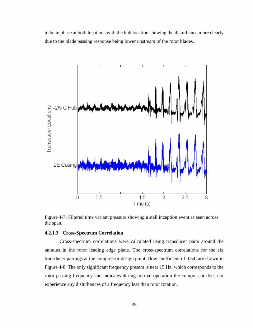
The pre-stall disturbance and rotating stall cell also impact the entire span, as seen
in Figure 4-7, which shows the hub transducer 40% rotor tip chord upstream compared to
the one over the rotor leading edge with both transducers being at the 90° circumferential
location for the same data set shown in Figure 4-6. The pre-stall disturbance was observed
Pre-stall
Additional flow breakdown
preceding stall
Rotating Stall
35
to be in phase at both locations with the hub location showing the disturbance more clearly
due to the blade passing response being lower upstream of the rotor blades.
Figure 4-7: Filtered time variant pressure showing a stall inception event as seen across
the span.
4.2.1.3 Cross-Spectrum Correlation
Cross-spectrum correlations were calculated using transducer pairs around the
annulus in the rotor leading edge plane. The cross-spectrum correlations for the six
transducer pairings at the compressor design point, flow coefficient of 0.54, are shown in
Figure 4-8. The only significant frequency present is near 15 Hz, which corresponds to the
rotor passing frequency and indicates during normal operation the compressor does not
experience any disturbances of a frequency less than rotor rotation.

36
Figure 4-8: Cross-spectrum correlation of circumferential transducer pairings in the rotor
leading edge plane at the design point.
The next set of cross-spectrum correlations are during the periodic disturbance at a
flow coefficient below 0.4. In Figure 4-9, a frequency is present at close to 6.8 Hz. This
frequency corresponds to the visible coherent low amplitude periodic disturbance. The
overall amplitude of the pre-stall disturbance is on the same order as the one per revolution
signature. After computing the phase angle and dividing by the transducer separation angle,
the number of nodes was computed to be 2 for each of the transducer sets. This indicates
that during the pre-stall disturbance the UKLSRC experiences a two node disturbance
traveling at near 23% rotor rotational speed. These findings agree with, and further
supplement, the hand calculations performed with the filtered time variant pressure.

37
Figure 4-9: Cross-spectrum correlation of circumferential transducer pairings in the rotor
leading edge plane.
The final set of circumferential cross-spectrum correlations occurs while the
UKLSRC experiences fully developed rotating stall. A frequency near 5.2 Hz is
prominently shown in Figure 4-10 while harmonics can be seen at the lower amplitudes.
The magnitude of the rotating stall cell is more than an order of magnitude beyond the pre-
stall disturbance and the rotor revolution signature. The number of cells at the fundamental
stall frequency was calculated to be 1 for each of the transducer pairings. This shows that
during fully developed rotating stall the UKLSRC experiences a single stall cell traveling
at near 35% rotor rotational speed, which is consistent with the results from the filtered
time variant pressure of Figure 4-4.
38
Figure 4-10: Cross-spectrum correlation of circumferential transducer pairings in the
rotor leading edge plane during fully developed rotating stall.
4.2.1.4 Spatial Fourier Transform
With transducers equally spaced around the entire annulus in the rotor leading edge
plane, a spatial Fourier transform was able to be conducted. For Figure 4-11, the
compressor was operating below a flow coefficient of 0.4 and the pre-stall disturbance
naturally transitioned into rotating stall. This is illustrated by a wavenumber of 2 being the
largest amplitude before stall initiation near 41 seconds in which afterwards the
wavenumber 1 becomes the predominant response. This can be related to the two node
disturbance prior to single rotating stall cell becoming developed. This is also in agreement
with the filtered time trace and cross-spectrum correlation results for the number of nodes
during each operating condition.
2nd
Harmonic 1st
Harmonic
3rd
Harmonic

39
Figure 4-11: Spatial Fourier transform of a stall inception event showing the 2 node
disturbance growing into a single rotating stall cell.
4.2.2 Axial Pressure Transducer Configuration
4.2.2.1 Flow Deviations
The trend present in the circumferential transducer configuration for the breakdown
of flow periodicity as stall is approached is mimicked for the axial transducer configuration
illustrated in Figure 4-12. While operating near the compressor design point with a flow
coefficient of 0.54, there is not much spread in the amount of flow deviation along the rotor
chord, but below a flow coefficient of 0.4 the breakdown at the rotor leading edge becomes
dominate.
40
Figure 4-12: Blade periodicity deviations along the rotor chord showing the highest flow
deviations occurring at the leading edge.
4.2.2.2 Time Dependent Pressures
The low-pass filtered time variant pressure measurements along the rotor chord
length are presented in Figure 4-13 while the compressor is operating during rotating stall.
It is evident that the stall cell is of enough size to impact the flow along the full length of
the rotor tip chord. Visual inspection of Figure 4-13 shows 10 to 11 stall cell signatures
over the two seconds for a frequency in the 5.25 Hz range, which is consistent for the
circumferential cross-spectrum correlation frequency of near 5.2 Hz.
41
Figure 4-13: Filtered time trace along the axial chord.
Prior to stall and at a flow coefficient below 0.4 the pre-stall disturbance can be
visually identified in the low-pass filtered time dependent pressure of Figure 4-14. This is
an indication that the perturbed velocity field coming into the rotors is impacting the flow
along the chord length and if a critical value is reached could lead to flow separating from
the surface leading to stall.

42
Figure 4-14: Filtered time dependent pressure showing the pre-stall disturbance along the
axial chord.
A stall inception event is shown in the low-pass filtered time trace in Figure 4-15.
At 0 seconds the compressor is operating with the modal disturbance and shortly after 0.5
seconds the rotating stall cell has been initiated elsewhere in the machine and it can be
shown to grow in amplitude and size as it matures.

43
Figure 4-15: Stall inception event as seen along the rotor axial chord.
4.2.2.3 Fourier Transforms
Due to the transducers being spaced along the axial chord and not circumferentially
spaced, cross-spectrum correlations were not able to be computed, but the Fourier
transform of the pressure signal could still be analyzed. The Fourier transform of the
pressure transducers while the compressor is operating at the design point, flow coefficient
0.54, is displayed in Figure 4-16. As with the cross-spectrum correlations of the
circumferential transducer configuration, there are no frequencies below rotor passing
frequency and the compressor is operating free of any disturbances.
44
Figure 4-16: Fourier transform of pressure transducers located along the axial chord at the
compressor design point.
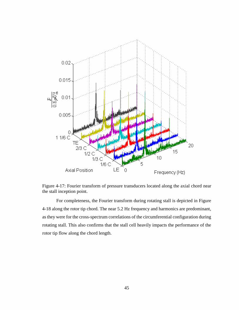
The Fourier transform of the time variant pressure measurements presented in
Figure 4-14 without the low-pass filtering is illustrated in Figure 4-17. The low amplitude
periodic disturbance has a frequency near 6.8 Hz. This is in agreement with the prior cross-
spectrum correlations performed with the circumferential pressure transducer arrangement.
This confirms that the pre-stall disturbance impacts the rotor tip flow along the full chord
length.
45
Figure 4-17: Fourier transform of pressure transducers located along the axial chord near
the stall inception point.
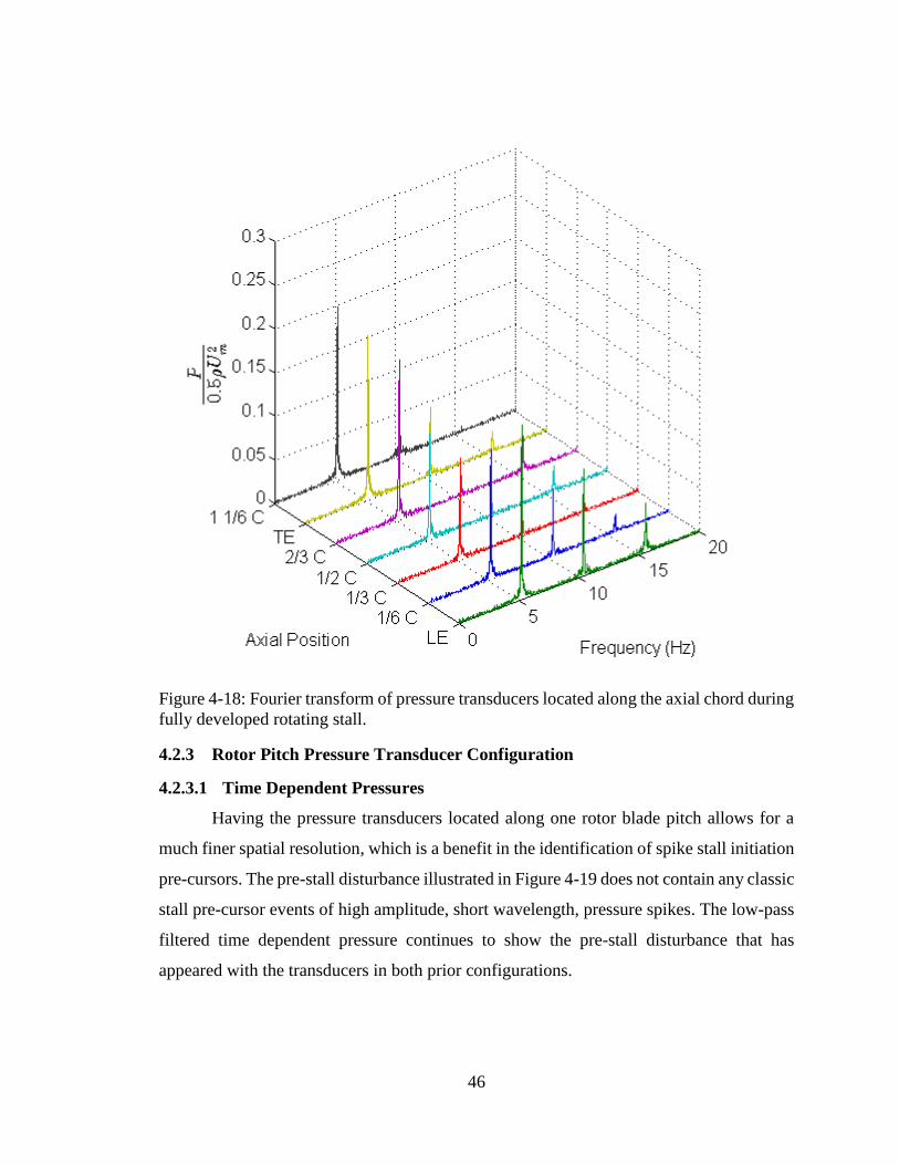
For completeness, the Fourier transform during rotating stall is depicted in Figure
4-18 along the rotor tip chord. The near 5.2 Hz frequency and harmonics are predominant,
as they were for the cross-spectrum correlations of the circumferential configuration during
rotating stall. This also confirms that the stall cell heavily impacts the performance of the
rotor tip flow along the chord length.
46
Figure 4-18: Fourier transform of pressure transducers located along the axial chord during
fully developed rotating stall.
4.2.3 Rotor Pitch Pressure Transducer Configuration
4.2.3.1 Time Dependent Pressures
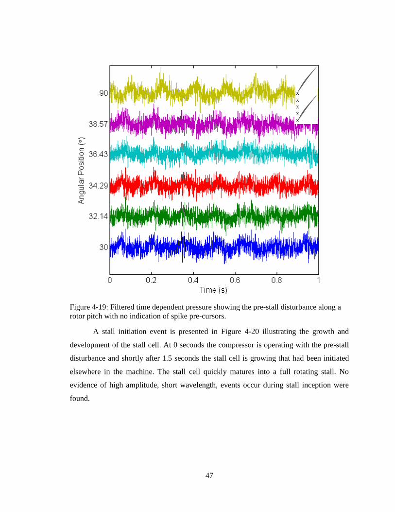
Having the pressure transducers located along one rotor blade pitch allows for a
much finer spatial resolution, which is a benefit in the identification of spike stall initiation
pre-cursors. The pre-stall disturbance illustrated in Figure 4-19 does not contain any classic
stall pre-cursor events of high amplitude, short wavelength, pressure spikes. The low-pass
filtered time dependent pressure continues to show the pre-stall disturbance that has
appeared with the transducers in both prior configurations.
47
Figure 4-19: Filtered time dependent pressure showing the pre-stall disturbance along a
rotor pitch with no indication of spike pre-cursors.
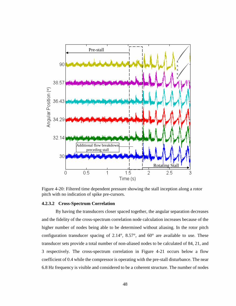
A stall initiation event is presented in Figure 4-20 illustrating the growth and
development of the stall cell. At 0 seconds the compressor is operating with the pre-stall
disturbance and shortly after 1.5 seconds the stall cell is growing that had been initiated
elsewhere in the machine. The stall cell quickly matures into a full rotating stall. No
evidence of high amplitude, short wavelength, events occur during stall inception were
found.
48
Figure 4-20: Filtered time dependent pressure showing the stall inception along a rotor
pitch with no indication of spike pre-cursors.
4.2.3.2 Cross-Spectrum Correlation
By having the transducers closer spaced together, the angular separation decreases
and the fidelity of the cross-spectrum correlation node calculation increases because of the
higher number of nodes being able to be determined without aliasing. In the rotor pitch
configuration transducer spacing of 2.14°, 8.57°, and 60° are available to use. These
transducer sets provide a total number of non-aliased nodes to be calculated of 84, 21, and
3 respectively. The cross-spectrum correlation in Figure 4-21 occurs below a flow
coefficient of 0.4 while the compressor is operating with the pre-stall disturbance. The near
6.8 Hz frequency is visible and considered to be a coherent structure. The number of nodes
Pre-stall
Additional flow breakdown
preceding stall
Rotating Stall
49
calculated from the cross-power spectrum, for each transducer separation angle, still
indicates that the pre-stall disturbance has 2 nodes.
Figure 4-21: Cross-spectrum correlations along a rotor pitch during the pre-stall
disturbance.
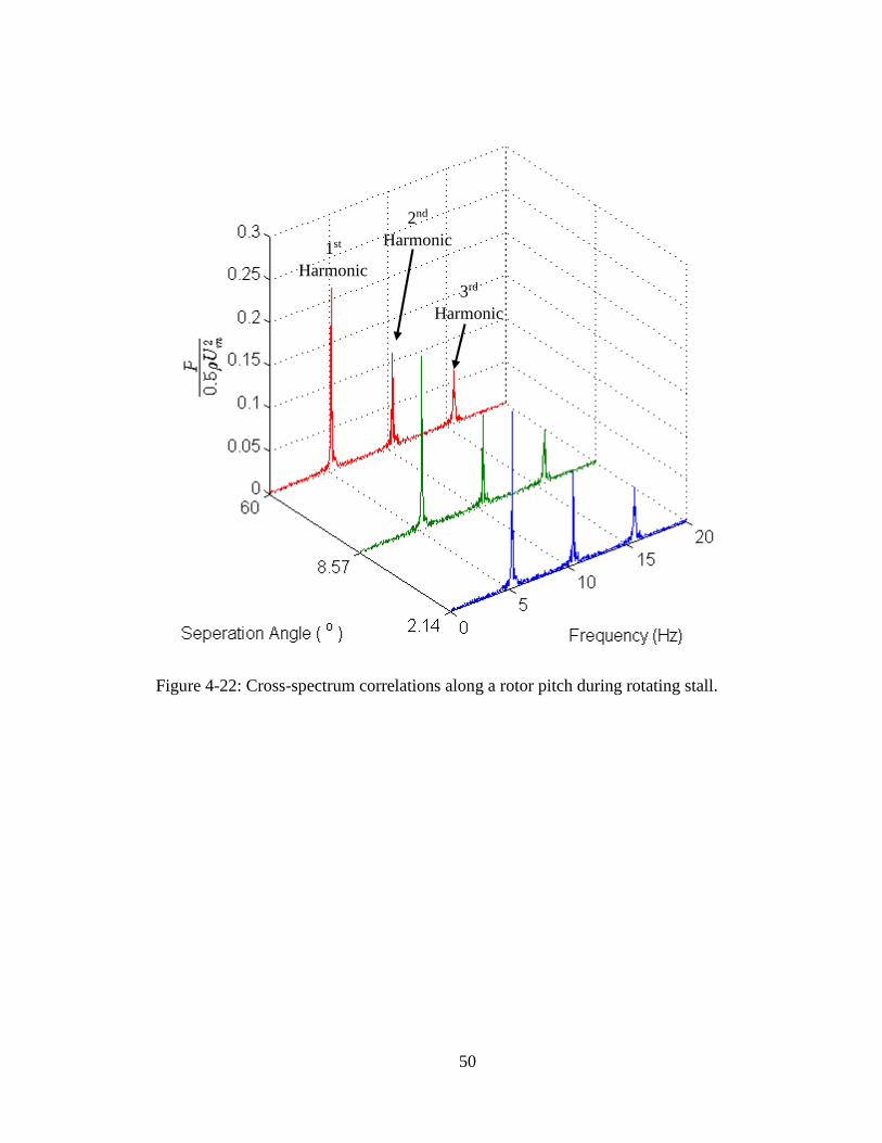
To verify the number of stall cells present during rotating stall, the cross-spectrum
correlations were performed during rotating stall with the rotor pitch transducer
configuration. The fundamental frequency response in Figure 4-22 is near 5.2 Hz and
corresponds to the previously established stall cell frequency. Using the phase angle of the
cross-power spectrum, the rotating stall has a single node.
50
Figure 4-22: Cross-spectrum correlations along a rotor pitch during rotating stall.
2nd
Harmonic 1st
Harmonic
3rd
Harmonic
51
4.3 Discussion
The data analysis consists of analyzing the breakdown of blade periodicity in terms
of a standard deviation from the mean across a rotor revolution, cross-spectrum correlations
between transducer pairings to determine coherent structures in the frequency spectrum,
spatial Fourier transforms over time of the equally spaced circumferential transducers, and
time traces of the pressure signals low-passed filtered at half of the blade passing
frequency. These data analysis techniques were utilized to quantify the stall inception
characteristics of the UKLSRC.
The breakdown of flow periodicity in the UKLSRC increases as the flow
coefficient approaches the stall inception point. This is in good agreement with prior work
by Young et al. (2011) who demonstrated a rise in the amount of flow irregularity as stall
is approached in a single-stage low-speed compressor. The UKLSRC has a small mean tip
clearance with a low level of eccentricity and the circumferential flow deviation
measurements showing the same rate of growth support the findings of Young et al. (2011)
for concentric compressors. The rotor leading edge transducer location showed the most
sensitivity in regards to the breakdown of flow periodicity.
The UKLSRC behaves dimensionally similar at multiple rotational speeds. Steady
state compressor characteristics show a near zero slope at the stall line while running at
multiple rotational speeds and the pre-stall disturbance occurring below a flow coefficient
of 0.4. The near zero slope is typical for a compressor that experiences a modal stall
inception.
The cross-spectrum correlations were applied to the circumferential and rotor pitch
transducer configurations, while standard Fourier transforms were applied to the axial
chord configuration. The frequency spectrums for all transducer configurations were able
to identify a pre-stall disturbance with a frequency near 6.8 Hz. By using the cross-
spectrum correlations, the number of pre-stall nodes was found to be two. This corresponds
to a two node pre-stall disturbance traveling near 23% rotor rotational speed. The pre-stall
disturbance impacted the compressor span as seen from the frequency spectrum response
of the pressure transducer located upstream of the rotors in the hub below a flow coefficient
of 0.4. The frequency spectrums for all transducer configurations were able to detect the
stall frequency of near 5.2 Hz. By using the cross-spectrum correlations the number of stall
52
cells was found to be one. This corresponds to a single stall cell traveling near 35% rotor
rotational speed.
The low-pass filtered pressure traces allowed for easier visualization of the pre-stall
disturbance. The low-pass filtering was also a requirement to perform the spatial Fourier
transform for the circumferential transducer configuration. The spatial Fourier transform
agreed with the number of nodes in the pre-stall disturbance and during rotating stall
obtained by the cross-spectrum correlation. No indication of spike stall with large
amplitude, short wavelength events were seen in the filtered pressure traces containing stall
inception.
The transition from the pre-stall disturbance to a rotating stall occurs due to the
change in incidence angle at the rotor leading edge. The pressure response can be correlated
to a change in velocity and this velocity change could cause a blade or series of blades to
have flow separation. If the amount of the flow separation is large enough to block the rotor
passage, the rotor blade will stall and the stall will propagate through the compressor in the
direction of rotation but at a slower speed.
All of the experimental results indicate the UKLSRC experiences a modal stall
inception due to the following characteristics: 1) the compressor characteristics curve has
a near zero positive slope at the stall inception point; 2) the coherent pre-stall disturbance
exists for more than one hundred rotor revolutions prior to stall; 3) the coherent pre-stall
disturbance is experienced across the span and through the entire annulus; 4) there is an up
shift of rotational speed between the pre-stall disturbance and the rotating stall cell.
53
5 CONCLUSIONS
The instrumentation, data acquisition system, data analysis, and operating
procedures were established to investigate the stall inception characteristics of the
UKLSRC with a mean tip clearance 0.64% with respect to annulus height. The time variant
instrumentation consisted of casing and hub mounted high frequency response pressure
transducers that were used to quantify the static pressures at various transducer locations.
The transducer configurations that were tested include being arranged equally spaced
circumferentially around the annulus over the rotor leading edges, equally spaced within
one rotor pitch in the leading edge plane, and equally spaced along the rotor axial chord
length. The data acquisition system was created using the Data Acquisition Toolbox in
MATLAB, which allows for continuous recording of the time variant data and TCP/IP
connection to the Scanivavle pressure scanning unit. MATLAB was chosen due to the easy
expandability in number of data acquisition channels.
The following conclusions can be drawn from this investigation:
1) Cross-spectrum correlations and spatial Fourier transforms are able to identify coherent
structures and the number of nodes for modal stall inception. It is unclear if these
methods would be applicable to spike stall inception.
2) For a limited number of pressure transducers, cross-spectrum correlations prove more
effective than spatial Fourier transforms due to the spacing requirements of the spatial
Fourier transform during modal stall inception.
3) Two pressure transducers in the same plane can be spaced close enough together to
provide adequate anti-aliasing to determine the number of nodes.
4) The amount of breakdown of flow periodicity increases with a decrease in flow
coefficient.
5) The UKLSRC experiences a modal stall inception.
Being able to better understand stall inception is important to the development and
continued use of gas turbine engines. Greater understanding and control over stall can
significantly reduce the cost in the design and development of turbomachines. Active stall
control could help push gas turbine engines to new levels of performance as well as extend
the gas turbine life cycle by reducing stall related fatigue.

54
A single experimental study has been presented that showcases the stall inception
characteristics of the UKLSRC. The data analysis techniques present can be applied to any
other low or high speed compressions systems to further study stall inception.
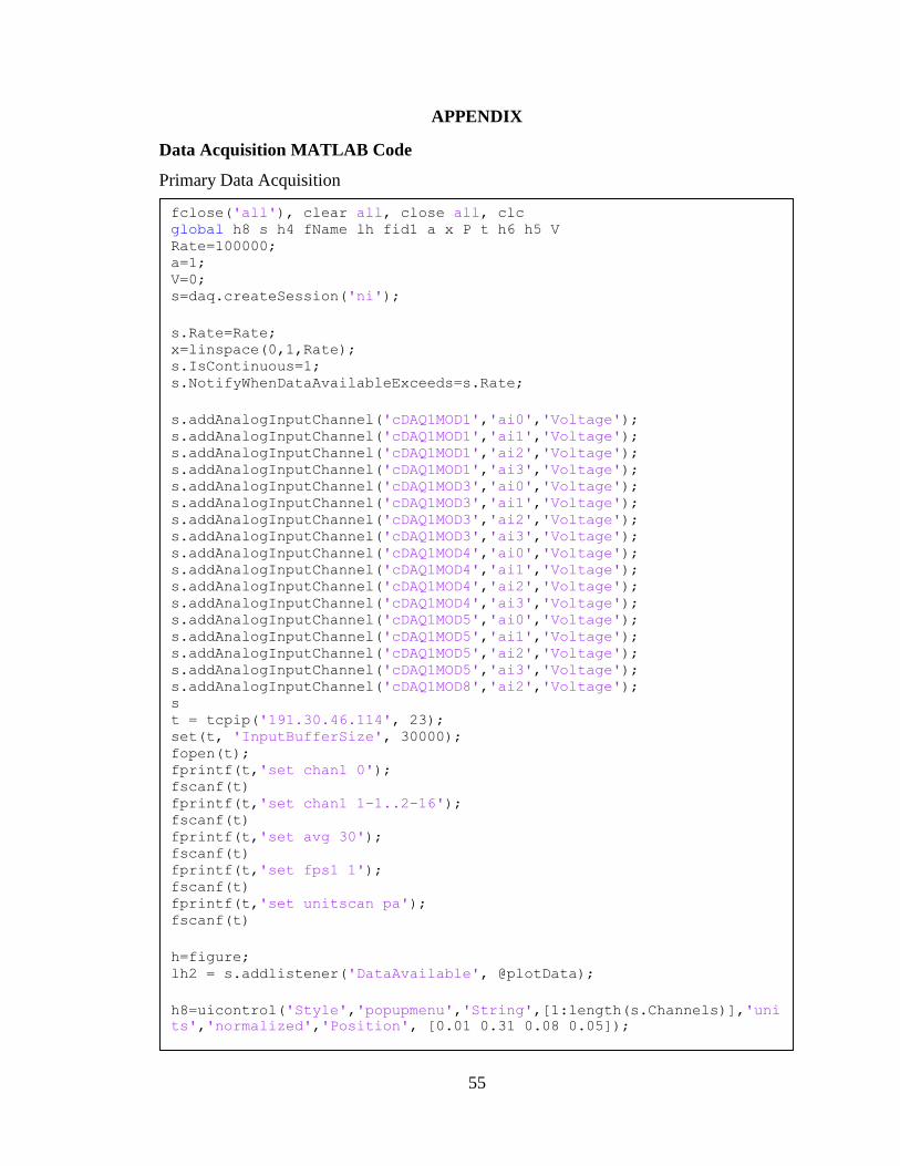
55
APPENDIX
Data Acquisition MATLAB Code
Primary Data Acquisition
fclose('all'), clear all, close all, clc global h8 s h4 fName lh fid1 a x P t h6 h5 V Rate=100000; a=1; V=0; s=daq.createSession('ni');
s.Rate=Rate; x=linspace(0,1,Rate); s.IsContinuous=1; s.NotifyWhenDataAvailableExceeds=s.Rate;
s.addAnalogInputChannel('cDAQ1MOD1','ai0','Voltage'); s.addAnalogInputChannel('cDAQ1MOD1','ai1','Voltage'); s.addAnalogInputChannel('cDAQ1MOD1','ai2','Voltage'); s.addAnalogInputChannel('cDAQ1MOD1','ai3','Voltage'); s.addAnalogInputChannel('cDAQ1MOD3','ai0','Voltage'); s.addAnalogInputChannel('cDAQ1MOD3','ai1','Voltage'); s.addAnalogInputChannel('cDAQ1MOD3','ai2','Voltage'); s.addAnalogInputChannel('cDAQ1MOD3','ai3','Voltage'); s.addAnalogInputChannel('cDAQ1MOD4','ai0','Voltage'); s.addAnalogInputChannel('cDAQ1MOD4','ai1','Voltage'); s.addAnalogInputChannel('cDAQ1MOD4','ai2','Voltage'); s.addAnalogInputChannel('cDAQ1MOD4','ai3','Voltage'); s.addAnalogInputChannel('cDAQ1MOD5','ai0','Voltage'); s.addAnalogInputChannel('cDAQ1MOD5','ai1','Voltage'); s.addAnalogInputChannel('cDAQ1MOD5','ai2','Voltage'); s.addAnalogInputChannel('cDAQ1MOD5','ai3','Voltage'); s.addAnalogInputChannel('cDAQ1MOD8','ai2','Voltage'); s
t = tcpip('191.30.46.114', 23); set(t, 'InputBufferSize', 30000); fopen(t); fprintf(t,'set chan1 0'); fscanf(t) fprintf(t,'set chan1 1-1..2-16'); fscanf(t) fprintf(t,'set avg 30'); fscanf(t) fprintf(t,'set fps1 1'); fscanf(t) fprintf(t,'set unitscan pa'); fscanf(t)
h=figure; lh2 = s.addlistener('DataAvailable', @plotData);
h8=uicontrol('Style','popupmenu','String',[1:length(s.Channels)],'uni
ts','normalized','Position', [0.01 0.31 0.08 0.05]);
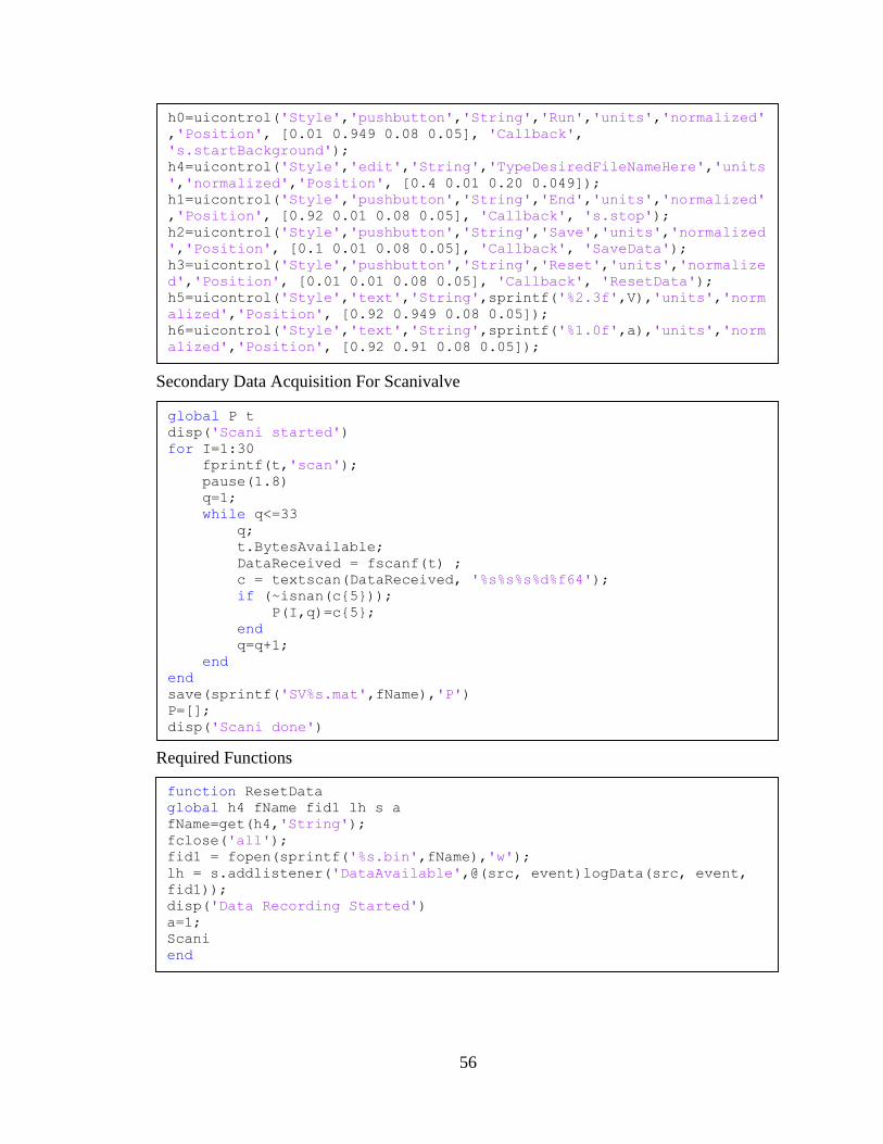
56
Secondary Data Acquisition For Scanivalve
Required Functions
h0=uicontrol('Style','pushbutton','String','Run','units','normalized'
,'Position', [0.01 0.949 0.08 0.05], 'Callback',
's.startBackground'); h4=uicontrol('Style','edit','String','TypeDesiredFileNameHere','units
','normalized','Position', [0.4 0.01 0.20 0.049]); h1=uicontrol('Style','pushbutton','String','End','units','normalized'
,'Position', [0.92 0.01 0.08 0.05], 'Callback', 's.stop'); h2=uicontrol('Style','pushbutton','String','Save','units','normalized
','Position', [0.1 0.01 0.08 0.05], 'Callback', 'SaveData'); h3=uicontrol('Style','pushbutton','String','Reset','units','normalize
d','Position', [0.01 0.01 0.08 0.05], 'Callback', 'ResetData'); h5=uicontrol('Style','text','String',sprintf('%2.3f',V),'units','norm
alized','Position', [0.92 0.949 0.08 0.05]); h6=uicontrol('Style','text','String',sprintf('%1.0f',a),'units','norm
alized','Position', [0.92 0.91 0.08 0.05]);
global P t disp('Scani started') for I=1:30 fprintf(t,'scan'); pause(1.8) q=1; while q<=33 q; t.BytesAvailable; DataReceived = fscanf(t) ; c = textscan(DataReceived, '%s%s%s%d%f64'); if (~isnan(c{5})); P(I,q)=c{5}; end q=q+1; end end save(sprintf('SV%s.mat',fName),'P') P=[]; disp('Scani done')
function ResetData global h4 fName fid1 lh s a fName=get(h4,'String'); fclose('all'); fid1 = fopen(sprintf('%s.bin',fName),'w'); lh = s.addlistener('DataAvailable',@(src, event)logData(src, event,
fid1)); disp('Data Recording Started') a=1; Scani end
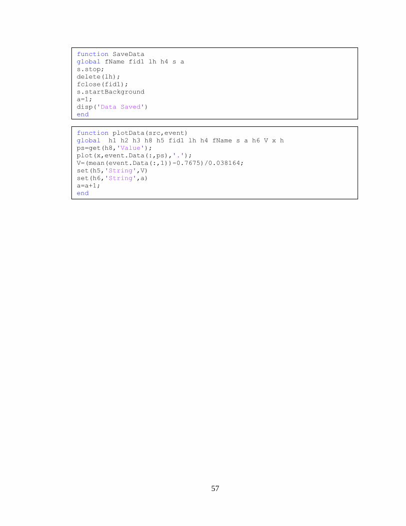
57
function SaveData global fName fid1 lh h4 s a s.stop; delete(lh); fclose(fid1); s.startBackground a=1; disp('Data Saved') end
function plotData(src,event) global h1 h2 h3 h8 h5 fid1 lh h4 fName s a h6 V x h ps=get(h8,'Value'); plot(x,event.Data(:,ps),'.'); V=(mean(event.Data(:,1))-0.7675)/0.038164; set(h5,'String',V) set(h6,'String',a) a=a+1; end
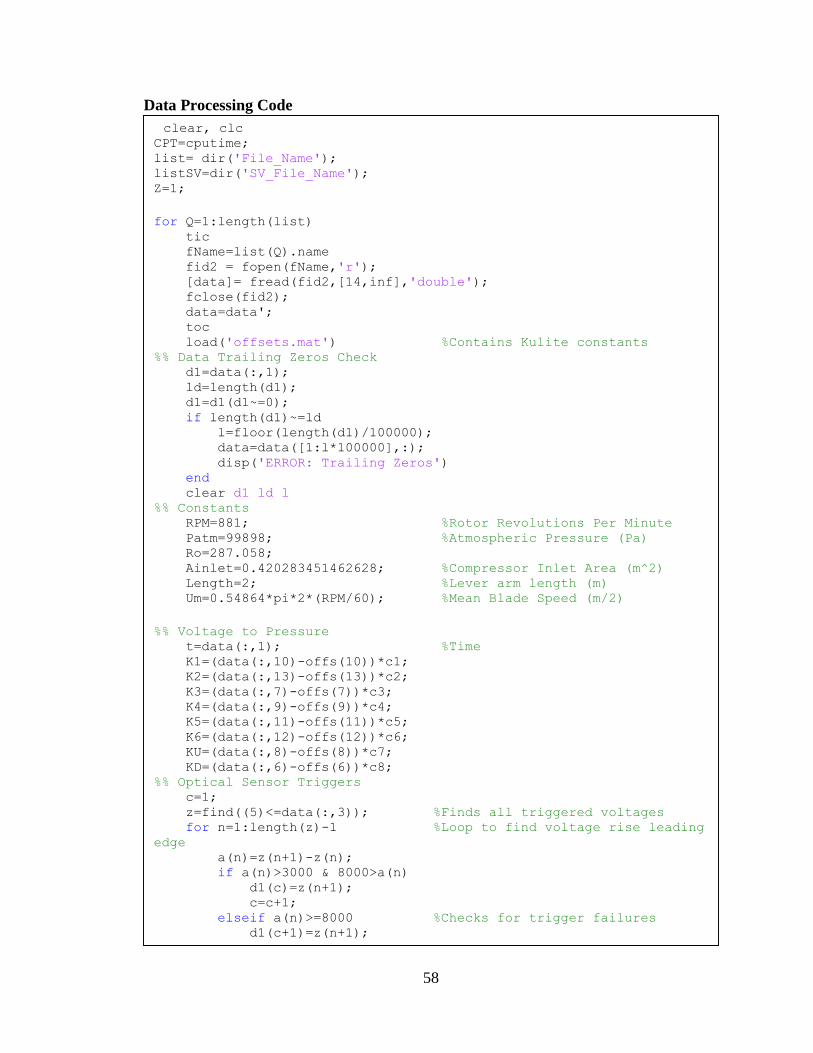
58
Data Processing Code
clear, clc CPT=cputime; list= dir('File_Name'); listSV=dir('SV_File_Name'); Z=1;
for Q=1:length(list) tic fName=list(Q).name fid2 = fopen(fName,'r'); [data]= fread(fid2,[14,inf],'double'); fclose(fid2); data=data'; toc load('offsets.mat') %Contains Kulite constants %% Data Trailing Zeros Check d1=data(:,1); ld=length(d1); d1=d1(d1~=0); if length(d1)~=ld l=floor(length(d1)/100000); data=data([1:l*100000],:); disp('ERROR: Trailing Zeros') end clear d1 ld l %% Constants RPM=881; %Rotor Revolutions Per Minute Patm=99898; %Atmospheric Pressure (Pa) Ro=287.058; Ainlet=0.420283451462628; %Compressor Inlet Area (m^2) Length=2; %Lever arm length (m) Um=0.54864*pi*2*(RPM/60); %Mean Blade Speed (m/2)
%% Voltage to Pressure t=data(:,1); %Time K1=(data(:,10)-offs(10))*c1; K2=(data(:,13)-offs(13))*c2; K3=(data(:,7)-offs(7))*c3; K4=(data(:,9)-offs(9))*c4; K5=(data(:,11)-offs(11))*c5; K6=(data(:,12)-offs(12))*c6; KU=(data(:,8)-offs(8))*c7; KD=(data(:,6)-offs(6))*c8; %% Optical Sensor Triggers c=1; z=find((5)<=data(:,3)); %Finds all triggered voltages for n=1:length(z)-1 %Loop to find voltage rise leading
edge a(n)=z(n+1)-z(n); if a(n)>3000 & 8000>a(n) d1(c)=z(n+1); c=c+1; elseif a(n)>=8000 %Checks for trigger failures d1(c+1)=z(n+1); d1(c)=round((d1(c-1)+d1(c+1))/2); c=c+2; disp 'Optical Sensor Failure' z(n) end end b=diff(d1); %Timing between Revolutions if Z==1
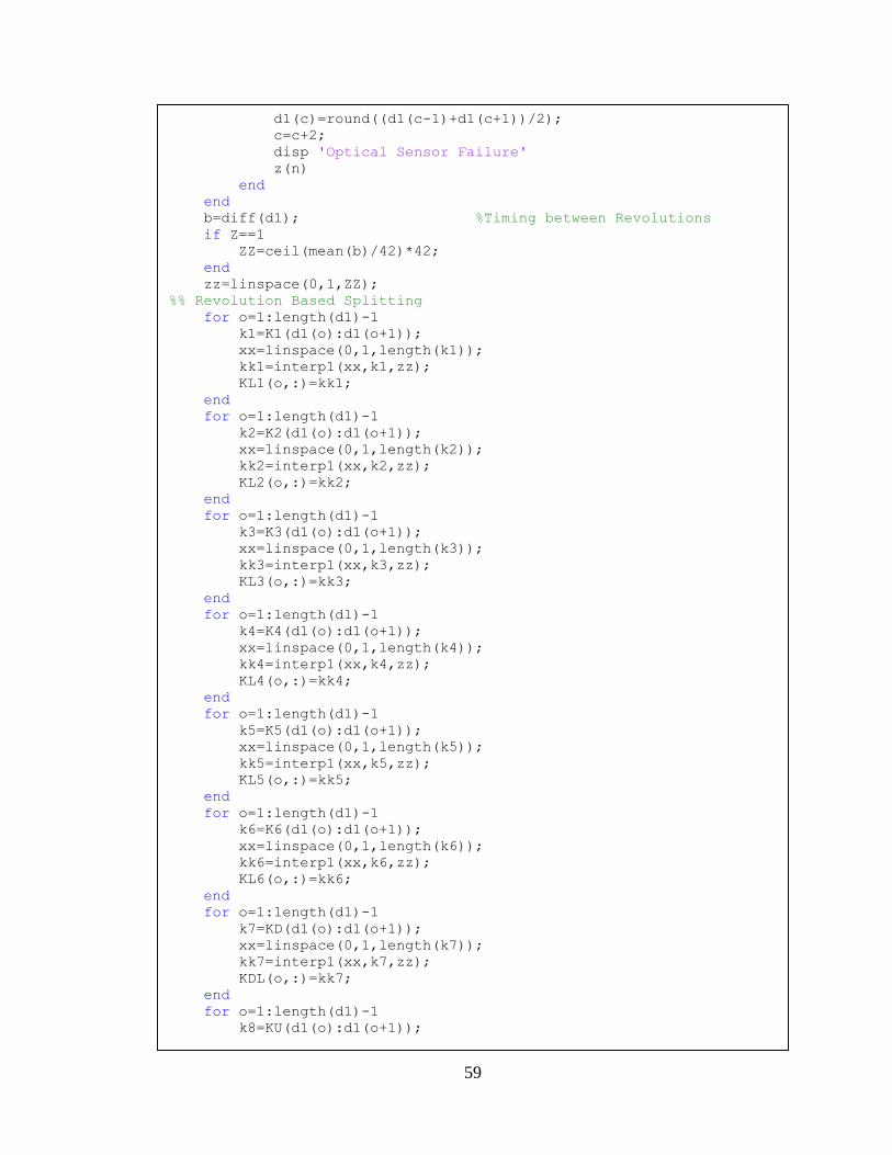
59
d1(c)=round((d1(c-1)+d1(c+1))/2); c=c+2; disp 'Optical Sensor Failure' z(n) end end b=diff(d1); %Timing between Revolutions if Z==1 ZZ=ceil(mean(b)/42)*42; end zz=linspace(0,1,ZZ); %% Revolution Based Splitting for o=1:length(d1)-1 k1=K1(d1(o):d1(o+1)); xx=linspace(0,1,length(k1)); kk1=interp1(xx,k1,zz); KL1(o,:)=kk1; end for o=1:length(d1)-1 k2=K2(d1(o):d1(o+1)); xx=linspace(0,1,length(k2)); kk2=interp1(xx,k2,zz); KL2(o,:)=kk2; end for o=1:length(d1)-1 k3=K3(d1(o):d1(o+1)); xx=linspace(0,1,length(k3)); kk3=interp1(xx,k3,zz); KL3(o,:)=kk3; end for o=1:length(d1)-1 k4=K4(d1(o):d1(o+1)); xx=linspace(0,1,length(k4)); kk4=interp1(xx,k4,zz); KL4(o,:)=kk4; end for o=1:length(d1)-1 k5=K5(d1(o):d1(o+1)); xx=linspace(0,1,length(k5)); kk5=interp1(xx,k5,zz); KL5(o,:)=kk5; end for o=1:length(d1)-1 k6=K6(d1(o):d1(o+1)); xx=linspace(0,1,length(k6)); kk6=interp1(xx,k6,zz); KL6(o,:)=kk6; end for o=1:length(d1)-1 k7=KD(d1(o):d1(o+1)); xx=linspace(0,1,length(k7)); kk7=interp1(xx,k7,zz); KDL(o,:)=kk7; end for o=1:length(d1)-1 k8=KU(d1(o):d1(o+1));
kk8=interp1(xx,k8,zz); KUL(o,:)=kk8; end %% Mean Pressure Profiles MP1=mean(KL1); MP2=mean(KL2); MP3=mean(KL3);
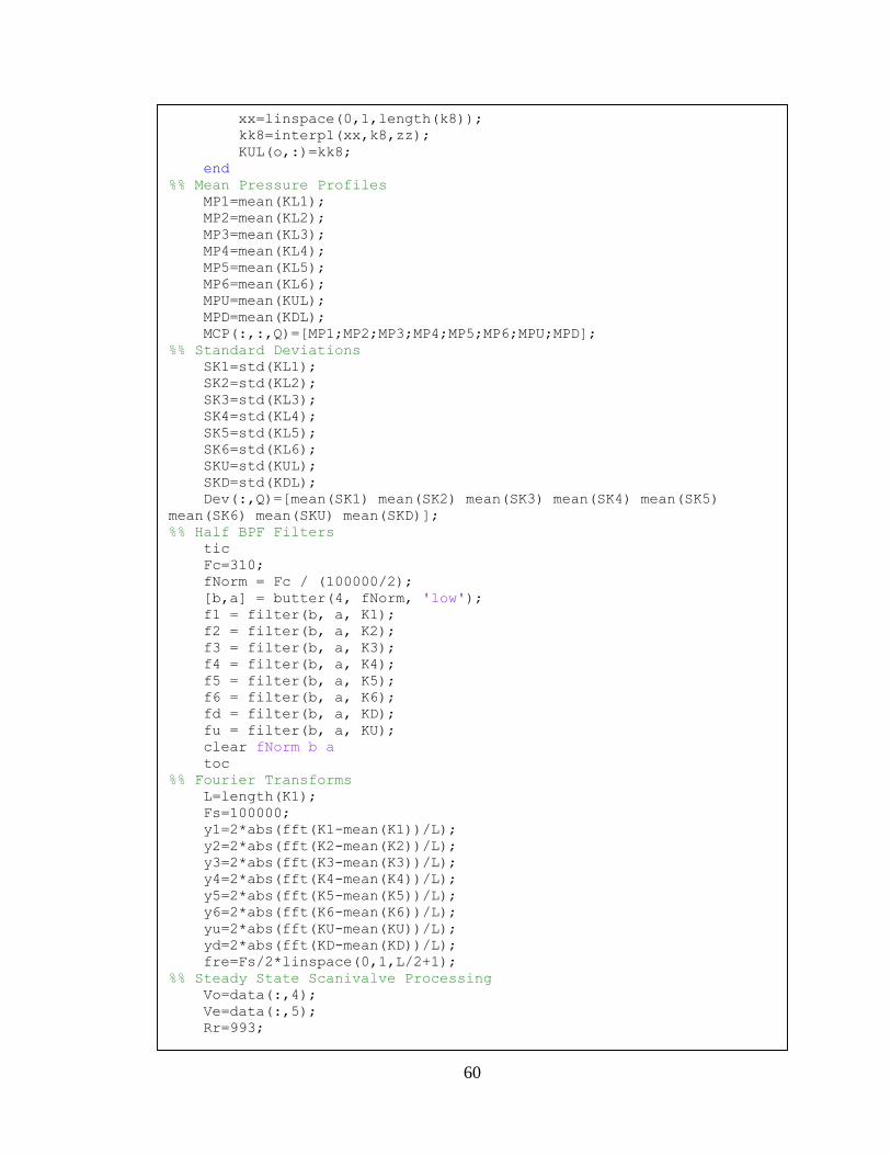
60
xx=linspace(0,1,length(k8)); kk8=interp1(xx,k8,zz); KUL(o,:)=kk8; end %% Mean Pressure Profiles MP1=mean(KL1); MP2=mean(KL2); MP3=mean(KL3); MP4=mean(KL4); MP5=mean(KL5); MP6=mean(KL6); MPU=mean(KUL); MPD=mean(KDL); MCP(:,:,Q)=[MP1;MP2;MP3;MP4;MP5;MP6;MPU;MPD]; %% Standard Deviations SK1=std(KL1); SK2=std(KL2); SK3=std(KL3); SK4=std(KL4); SK5=std(KL5); SK6=std(KL6); SKU=std(KUL); SKD=std(KDL); Dev(:,Q)=[mean(SK1) mean(SK2) mean(SK3) mean(SK4) mean(SK5)
mean(SK6) mean(SKU) mean(SKD)]; %% Half BPF Filters tic Fc=310; fNorm = Fc / (100000/2); [b,a] = butter(4, fNorm, 'low'); f1 = filter(b, a, K1); f2 = filter(b, a, K2); f3 = filter(b, a, K3); f4 = filter(b, a, K4); f5 = filter(b, a, K5); f6 = filter(b, a, K6); fd = filter(b, a, KD); fu = filter(b, a, KU); clear fNorm b a toc %% Fourier Transforms L=length(K1); Fs=100000; y1=2*abs(fft(K1-mean(K1))/L); y2=2*abs(fft(K2-mean(K2))/L); y3=2*abs(fft(K3-mean(K3))/L); y4=2*abs(fft(K4-mean(K4))/L); y5=2*abs(fft(K5-mean(K5))/L); y6=2*abs(fft(K6-mean(K6))/L); yu=2*abs(fft(KU-mean(KU))/L); yd=2*abs(fft(KD-mean(KD))/L); fre=Fs/2*linspace(0,1,L/2+1); %% Steady State Scanivalve Processing Vo=data(:,4); Ve=data(:,5); Rr=993;
A=1.468*10^-3; B=2.383*10^-4; C=1.007*10^-7;
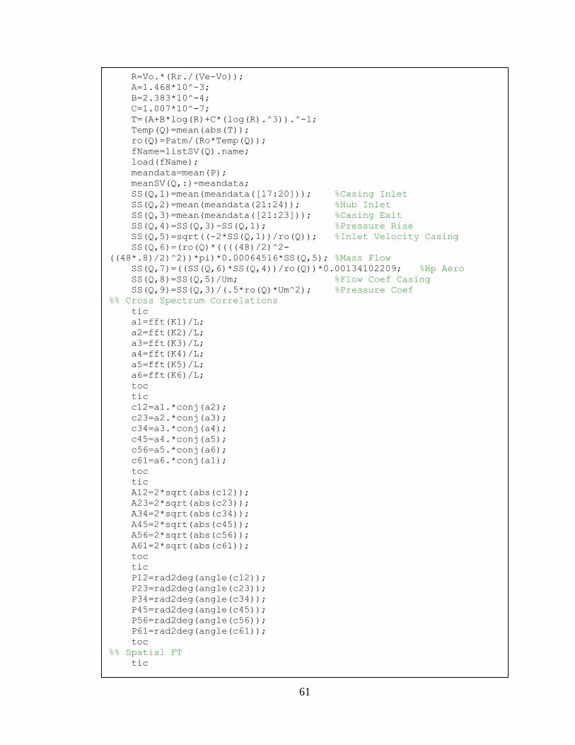
61
R=Vo.*(Rr./(Ve-Vo)); A=1.468*10^-3; B=2.383*10^-4; C=1.007*10^-7; T=(A+B*log(R)+C*(log(R).^3)).^-1; Temp(Q)=mean(abs(T)); ro(Q)=Patm/(Ro*Temp(Q)); fName=listSV(Q).name; load(fName); meandata=mean(P); meanSV(Q,:)=meandata; SS(Q,1)=mean(meandata([17:20])); %Casing Inlet SS(Q,2)=mean(meandata(21:24)); %Hub Inlet SS(Q,3)=mean(meandata([21:23])); %Casing Exit SS(Q,4)=SS(Q,3)-SS(Q,1); %Pressure Rise SS(Q,5)=sqrt((-2*SS(Q,1))/ro(Q)); %Inlet Velocity Casing SS(Q,6)=(ro(Q)*((((48)/2)^2-
((48*.8)/2)^2))*pi)*0.00064516*SS(Q,5); %Mass Flow SS(Q,7)=((SS(Q,6)*SS(Q,4))/ro(Q))*0.00134102209; %Hp Aero SS(Q,8)=SS(Q,5)/Um; %Flow Coef Casing SS(Q,9)=SS(Q,3)/(.5*ro(Q)*Um^2); %Pressure Coef %% Cross Spectrum Correlations tic a1=fft(K1)/L; a2=fft(K2)/L; a3=fft(K3)/L; a4=fft(K4)/L; a5=fft(K5)/L; a6=fft(K6)/L; toc tic c12=a1.*conj(a2); c23=a2.*conj(a3); c34=a3.*conj(a4); c45=a4.*conj(a5); c56=a5.*conj(a6); c61=a6.*conj(a1); toc tic A12=2*sqrt(abs(c12)); A23=2*sqrt(abs(c23)); A34=2*sqrt(abs(c34)); A45=2*sqrt(abs(c45)); A56=2*sqrt(abs(c56)); A61=2*sqrt(abs(c61)); toc tic P12=rad2deg(angle(c12)); P23=rad2deg(angle(c23)); P34=rad2deg(angle(c34)); P45=rad2deg(angle(c45)); P56=rad2deg(angle(c56)); P61=rad2deg(angle(c61)); toc %% Spatial FT tic
[b,a] = butter(4, fNorm, 'low'); g1 = filter(b, a, K1-mean(K1)); g2 = filter(b, a, K2-mean(K2)); g3 = filter(b, a, K3-mean(K3)); g4 = filter(b, a, K4-mean(K4)); g5 = filter(b, a, K5-mean(K5)); g6 = filter(b, a, K6-mean(K6));
62
Fc=9; fNorm = Fc / (100000/2); [b,a] = butter(4, fNorm, 'low'); g1 = filter(b, a, K1-mean(K1)); g2 = filter(b, a, K2-mean(K2)); g3 = filter(b, a, K3-mean(K3)); g4 = filter(b, a, K4-mean(K4)); g5 = filter(b, a, K5-mean(K5)); g6 = filter(b, a, K6-mean(K6)); gd = filter(b, a, KD-mean(KD)); gu = filter(b, a, KU-mean(KU)); clear fNorm b a toc sft0=zeros(1,length(K1)); sft1=sft0;sft2=sft1;sft3=sft2; tic for i=1:length(K1) temp=[g1(i) g2(i) g3(i) g4(i) g5(i) g6(i)]; fftem=fft(temp)/6; fftemp=2*abs(fftem); aft0(i)=rad2deg(angle(fftem(1))); aft1(i)=rad2deg(angle(fftem(2))); aft2(i)=rad2deg(angle(fftem(3))); aft3(i)=rad2deg(angle(fftem(4))); sft0(i)=fftemp(1); sft1(i)=fftemp(2); sft2(i)=fftemp(3); sft3(i)=fftemp(4); end toc %% Z=Z+1; clearvars -except Q Dev Ev list CPT Lc MCP diff O OO CR1 CR2 CR3
CR4 CR5 CR6 CRM Z SS ZZ listSV ro Temp meanSV Freq Amp RMSK1 RMSK2
RMSK3 RMSK4 RMSK5 RMSK6 RMSKU RMSKD end
63
REFERENCES
Beckwith, T., Marangoni. R., and Lienhard, J., Mechanical Measurements. Upper Saddle
River, NJ: Pearson/Prentice Hall, 2007.
Camp, T. and Day, I., “A Study of Spike and Modal Stall Phenomena in a Low-Speed
Axial Compressor,” Journal of Turbomachinery, Vol. 120, July, 1998, pp. 393-401.
Day, I.J., “Stall Inception in Axial Flow Compressors,” Journal of Turbomachinery, Vol.
115, Jan, 1993, pp. 1-9.
Fleeter, S., Bennett, W. A., and Jay, R. L., “The Time-Variant Aerodynamic Response of
a Stator Row Including the Effects of Airfoil Camber,” Journal of Engineering for Power,
Vol. 102, pp. 334-343.
Greitzer, M., “The Stability of Pumping Systems – The 1980 Freeman Scholar Lecture,”
Journal of Fluids Engineering, Vol. 103, 1981, pp. 193-242.
Kulite, “Miniature Ruggedized Pressure Transducer XT-190 (M) Series,” Web, April,
2014.
McDougall, N., Cumpsty, N., and Hynes, T., “Stall Inception in Axial Compressors,”
Journal of Turbomachinery, Vol. 112, Jan, 1990, pp. 116-125.
Moore, F. and Greitzer, E., “A Theory of Post-Stall Transients in Axial Compression
Systems: Part I-Development of Equations,” Journal of Engineering for Gas Turbines and
Power, Vol. 108, Jan, 1986, pp. 68-76.
Stenning, A., “Rotating Stall and Surge,” Journal of Fluids Engineering, Vol. 102, March,
1980, pp. 14-20.
Young, A., Day, I., and Pullan, G., “Stall Warning By Blade Pressure Signature Analysis,”
Proceedings of ASME Turbo Expo 2001, GT2011-45850.

64
VITA
Name: Bradley David Butler
Place of Birth: Paducah, Kentucky
Education:
Bachelor of Science in Mechanical Engineering, University of Kentucky, 2012
Professional positions held:
Teaching Assistant, University of Kentucky, Spring 2014
Graduate Research Assistant, University of Kentucky, 2012-2014
Undergraduate Research Assistant, University of Kentucky, 2010-2012
Scholastic honors:
Graduated University of Kentucky Magna Cum Laude
NASA Kentucky EPSCoR Space Grant recipient
Professional Publications:
Butler, B. and Capece, V., 2014, “Unsteady Pressure Measurements of a Low-Speed
Single-Stage Axial-Flow Compressor Near Stall,” Presentations 39th Dayton-
Cincinnati Aerospace Science Symposium.
Whipple, W., Butler, B., Sterrie, C., and Seay, J., 2013, “A Sustainable Low Cost Process
For The Production Of Biodiesel Suitable For Underdeveloped Regions,” Journal
of Green Building, Vol. 8, No3. pp. 140-155.
Butler, B. and Capece, V., 2013, “Casing Dynamic Pressure Measurements of an Axial
Flow Compressor Near Stall,” KY EPSCoR Annual Conference.
Butler, B. and Capece, V., 2013, “Time-dependent Shroud Pressure Measurements of a
Single-stage Compressor Near Rotating Stall Inception,” Presentations 38th
Dayton-Cincinnati Aerospace Science Symposium.
Seay, J., Zama, I., and Butler, B., 2012, “International Partnership Helping to Bring
Appropriate Biofuel Technology to Rural Cameroon,” International Journal of
Service Learning in Engineering, Vol. 7, No. 2.
Butler, B. and Capece, V., 2012, “Performance Measurements of a Low-Speed Single-
Stage Axial-Flow Compressor,” AIAA Paper No. AIAA-2012-3726.
Butler, B. and Capece, V., 2012, “Performance Measurements of the University of
Kentucky Low-Speed Axial-Flow Compressor,” Presentations 37th Dayton-
Cincinnati Aerospace Science Symposium.

65
Butler, B., Sterrie, C., and Whipple, W., 2012, “Cameroon Biodiesel Project,” Papers
MESCON, University of Evansville.
Butler, B., 2012, “Optimization of a Rotor Blade Vibration Control System,” Presentations
MESCON, University of Evansville.