Tutorial for QuantEvIcy plugin

Intracellularevents

0

0.01

0.02

Radial distribution

0

0.01

0.01

Angular distribution

0

0.1

0.2

0.3

In-depth distribution

Condition 1 Condition 2

�4

�2

0

2

4

6

Radius Angle Depth

�4

�2

0

2

4

6

Radius Angle Depth

�4

�2

0

2

4

6

Radius Angle Depth

�4

�2

0

2

4

6

Radius Angle Depth

�4

�2

0

2

4

6

Radius Angle Depth

�4

�2

0

2

4

6

Radius Angle Depth

�4

�2

0

2

4

6

Radius Angle Depth

�4

�2

0

2

4

6

Radius Angle Depth

�4

�2

0

2

4

6

Radius Angle Depth

0 2 4 60

0.1

0.2

�4

�2

0

2

4

6

Radius Angle Depth

�4

�2

0

2

4

6

Radius Angle Depth

�4

�2

0

2

4

6

Radius Angle Depth

�4

�2

0

2

4

6

Radius Angle Depth

�4

�2

0

2

4

6

Radius Angle Depth

�4

�2

0

2

4

6

Radius Angle Depth

�4

�2

0

2

4

6

Radius Angle Depth

�4

�2

0

2

4

6

Radius Angle Depth

�4

�2

0

2

4

6

Radius Angle Depth

�4

�2

0

2

4

6

Radius Angle Depth

�4

�2

0

2

4

6

Radius Angle Depth

*

0

0.01

0.02

Radial distribution

0

0.01

0.01

Angular distribution

0

0.1

0.2

0.3

In-depth distribution

Condition 1 Condition 2

0

0.01

0.02

Radial distribution

0

0.01

0.01

Angular distribution

0

0.1

0.2

0.3

In-depth distribution

Condition 1 Condition 2

0

0.01

0.02

Radial distribution

0

0.01

0.01

Angular distribution

0

0.1

0.2

0.3

In-depth distribution

p-value= 0.4816 p-value= 0.7853 p-value= 0.0094

Condition 1 Condition 2

0

0.01

0.02

Radial distribution

0

0.01

0.01

Angular distribution

0

0.1

0.2

0.3

In-depth distribution

p-value= 0.4816 p-value= 0.7853 p-value= 0.0094

Condition 1 Condition 2�4

�2

0

2

4

6

Radius Angle Depth

�4

�2

0

2

4

6

Radius Angle Depth

�4

�2

0

2

4

6

Radius Angle Depth

�4

�2

0

2

4

6

Radius Angle Depth

�4

�2

0

2

4

6

Radius Angle Depth

�4

�2

0

2

4

6

Radius Angle Depth

Spa/aldistribu/onanalysis

Weightedcylindricalhistogramsanddensi/es

Condi/ondistancesandsta/s/calanalysis

Uniformityanalysis

Entropymap

Pointdefiningthemostuniformangulardistribu/on

Segmenta/on/objectcomponent TrajectoriesAnyeventwith

spa/alcoordinates

NDimages

QuantEv

�4

�2

0

2

4

6

Radius Angle Depth

�4

�2

0

2

4

6

Radius Angle Depth

0

0.01

0.02

Radial distribution

0

0.01

0.01

Angular distribution

0

0.1

0.2

0.3

In-depth distribution

p-value= 0.4816 p-value= 0.7853 p-value= 0.0094

Condition 1 Condition 2

0

0.01

0.02

Radial distribution

0

0.01

0.01

Angular distribution

0

0.1

0.2

0.3

In-depth distribution

p-value= 0.4816 p-value= 0.7853 p-value= 0.0094

Condition 1 Condition 2

0

0.01

0.02

Radial distribution

0

0.01

0.01

Angular distribution

0

0.1

0.2

0.3

In-depth distribution

p-value= 0.4816 p-value= 0.7853 p-value= 0.0094

Condition 1 Condition 2

0

0.01

0.02

Radial distribution

0

0.01

0.01

Angular distribution

0

0.1

0.2

0.3

In-depth distribution

p-value= 0.4816 p-value= 0.7853 p-value= 0.0094

Condition 1 Condition 2

Contents

1 Introduction to QuantEv modules 31.1 QuantEv-Densities . . . . . . . . . . . . . . . . . . . . . . . . . . . . . . . . . . . . . . . 3

1.1.1 Inputs . . . . . . . . . . . . . . . . . . . . . . . . . . . . . . . . . . . . . . . . . . 31.1.2 Output . . . . . . . . . . . . . . . . . . . . . . . . . . . . . . . . . . . . . . . . . 5

1.2 QuantEv-Test . . . . . . . . . . . . . . . . . . . . . . . . . . . . . . . . . . . . . . . . . . 51.2.1 Inputs . . . . . . . . . . . . . . . . . . . . . . . . . . . . . . . . . . . . . . . . . . 51.2.2 Output . . . . . . . . . . . . . . . . . . . . . . . . . . . . . . . . . . . . . . . . . 5

1.3 QuantEv-Uniformity . . . . . . . . . . . . . . . . . . . . . . . . . . . . . . . . . . . . . . 51.3.1 Inputs . . . . . . . . . . . . . . . . . . . . . . . . . . . . . . . . . . . . . . . . . . 61.3.2 Outputs . . . . . . . . . . . . . . . . . . . . . . . . . . . . . . . . . . . . . . . . . 6

2 Test cases 72.1 Cell shape influence . . . . . . . . . . . . . . . . . . . . . . . . . . . . . . . . . . . . . . 7

2.1.1 Data . . . . . . . . . . . . . . . . . . . . . . . . . . . . . . . . . . . . . . . . . . . 72.1.2 Step-by-step analysis . . . . . . . . . . . . . . . . . . . . . . . . . . . . . . . . . . 72.1.3 Results . . . . . . . . . . . . . . . . . . . . . . . . . . . . . . . . . . . . . . . . . 9

2.2 Distribution comparison and visualization . . . . . . . . . . . . . . . . . . . . . . . . . . 92.2.1 Data . . . . . . . . . . . . . . . . . . . . . . . . . . . . . . . . . . . . . . . . . . . 92.2.2 Step-by-step analysis . . . . . . . . . . . . . . . . . . . . . . . . . . . . . . . . . . 92.2.3 Results . . . . . . . . . . . . . . . . . . . . . . . . . . . . . . . . . . . . . . . . . 10

2.3 Uniformity analysis . . . . . . . . . . . . . . . . . . . . . . . . . . . . . . . . . . . . . . . 102.3.1 Data . . . . . . . . . . . . . . . . . . . . . . . . . . . . . . . . . . . . . . . . . . . 102.3.2 Step-by-step analysis . . . . . . . . . . . . . . . . . . . . . . . . . . . . . . . . . . 112.3.3 Results . . . . . . . . . . . . . . . . . . . . . . . . . . . . . . . . . . . . . . . . . 11

2

This document is a tutorial for using QuantEv plugin with Icy. QuantEv is a fully automatic andnon-parametric framework divided into three distinct operations:

• QuantEv-Densities: from an input image (2D, 3D, 2D+t or 3D+t), QuantEv-Densities computeshistograms and densities in the cylindrical, spherical or Cartesian coordinate system,

• QuantEv-Test: from an input text file corresponding to densities, QuantEv-Test applies a pairedWilcoxon signed-rank test between the replicates of each condition,

• QuantEv-Uniformity: from an input image (2D, 3D, 2D+t or 3D+t), QuantEv-Uniformity findsthe reference point in the image corresponding to the most uniform angular distribution ofevents.

To show how to use QuantEv Icy plugin, we propose in this tutorial to apply the different functionalitiesof QuantEv on synthetic simulated image sequences.

1 Introduction to QuantEv modules

1.1 QuantEv-Densities

When you open QuantEv plugin, you obtain the interface shown in Fig. 1.

1.1.1 Inputs

• Input imageThe input image corresponds to the image for which you want to analyze the spatial distribution. Itcan be a fluorescence microscopy image in which case you will analyze the intensity distribution.Most of the time, it will be a pre-processed image, e.g. segmented particles. This input ismandatory.

• Channel in input image used for analysisThis input allows you to choose the channel of the image for which you want to analyze the spatialdistribution.

• Cell maskThe cell mask enables to take into account the cell shape in the spatial distribution analysis. Inthis mask, you have to define an intensity superior to 0 in the cell and equal to 0 outside the cell.This input is optional.

• Exclusion maskThe exclusion mask allows you to remove a region inside the cell where no event of interest occurs.In this mask, you have to define an intensity superior to 0 in the region in the cell that is excludedfrom the analysis. This input is optional.

• Coordinate system for QuantEvYou can choose a cylindrical, spherical or a Cartesian coordinate system, as well as analyzing thespatial distribution of the events with respect to their distance to the cell border.

• X coordinate of the system centerY coordinate of the system centerZ coordinate of the system center (for spherical coordinate system)The coordinates of the coordinate system center can be given to QuantEv. If not (-1), the cellcenter is considered as coordinate system center.

3

Figure 1: Screenshot of QuantEv-Densities.

• X coordinate of a point located on the polar/colatitude/X axisY coordinate of a point located on the polar/colatitude/X axisThe polar/azimuthal/X axis is defined by the line between the reference center and the coordinatesof a point on this axis. If not given (-1), the horizontal line starting from the reference point tothe right is defined as the polar/azimuthal/X axis.

• Consider intensity as weightThe intensity can be taken into account as weight for histograms and densities in the spatialdistributions.

• Output xls fileThe output xls file name has to be defined to export the results.

• Number of bins for radius/abscissa/distanceNumber of bins for polar angle/colatitude/ordinateNumber of bins for depth/azimuth angleThe ouput specifications allow to define the number of bins for each component.

4

Figure 2: Screenshot of QuantEv-Test.

1.1.2 Output

The output of QuantEv-Densities is a xls file containing the histograms and the densities. In this file,each worksheet has an explicit name.

1.2 QuantEv-Test

When you select QuantEv-Test in the field Mode for QuantEv, you obtain the interface shown in Fig. 2.

1.2.1 Inputs

• Input xls file for statistical analysisIn this xls file, each column corresponds to one image. The first row of the file contains thedifferent conditions. For a given condition, all the replicated experiments must have the samecondition identification.

• Worksheet to consider in the xls fileThis parameter allows you to select the worksheet in the xls file for which you want to apply astatistical analysis.

• DistributionThe distribution is circular for angular distributions and linear for the other distributions.

• Output xls fileThe output xls file name has to be defined to export the p-values obtained with a paired Wilcoxonsigned-rank test for every pair of conditions.

1.2.2 Output

The output xls file contains the p-values for every pair of conditions.

1.3 QuantEv-Uniformity

When you select QuantEv-Uniformity in the field Mode for QuantEv, you obtain the interface shown inFig. 3.

5

Figure 3: Screenshot of QuantEv-Uniformity.

1.3.1 Inputs

• Input imageThe input image is the image for which you want to estimate the point that gives the most uniformangular distribution. This input is mandatory.

• Channel in input image used for analysisThis input allows you to choose the channel of the image for which you want to analyze the spatialdistribution.

• Cell maskThe cell mask allows to remove the region that is out of the cell from the analysis. In this mask,you have to define an intensity superior to 0 in the cell and equal to 0 outside the cell. This inputis optional.

• Output xls fileThe output xls file name has to be defined to export the coordinates of the point(s) giving themost uniform angular distribution(s).

• Uniformity analysis for the whole sequence or at each time stepIn case of an image sequence, you can estimate a reference point for the whole sequence or at eachtime step.

• Compute entropy mapYou can get an entropy map as the point with the most uniform angular distribution is definedas the reference point with the maximum entropy for angular distribution. However, getting theentropy map will extend computation time as entropy is computed for each point while a bisectionmethod is used otherwise to speed up the computation.

1.3.2 Outputs

The output xls file contains the coordinates of the point that gives the most uniform angular distribution,over the whole sequence or at each time step. The entropy map is also given if required by the user.

6

2 Test cases

2.1 Cell shape influence

To illustrate the interest of the input cell mask and the region in the cell excluded from the analysis inQuantEv-Densities, we propose to analyze the spatial distribution of the same input image sequences

i) without a cell mask,

ii) with a cell mask,

iii) with a cell mask and a region excluded from the analysis.

2.1.1 Data

Let us start with particles uniformly distributed over 16 different paths from the center to the pe-riphery of square shaped-cells (see Fig. 4 first row). 10 simulations are available on the iMANAGEdatabase at https://cid.curie.fr/iManage/standard/login.html with username public and pass-word Welcome!1 in the project entitled QuantEv-Data (squaredShapedCell uniformDistribution 01.tif tosquaredShapedCell uniformDistribution 10.tif). The input cell mask and the region in the cell excludedfrom the analysis are also available on the iMANAGE database (squareShapedCellMask.pgm and square-ShapedCell regionExcludedFromTheAnalysis.pgm).

2.1.2 Step-by-step analysis

1 Select QuantEv-Densities in the field Mode for QuantEv

2 Open the image sequence entitled squaredShapedCell uniformDistribution 01.tif

3 Select squaredShapedCell uniformDistribution 01.tif as Input image

4 Change the number of bins for polar angle to 16 as only 16 paths around the reference center areused by the particles in the simulations

5 Select an output file name in the field Output cylindrical xls file

6 Push the play button to start the analysis

7 Repeat steps 2;3;6 for the 9 other image sequences (squaredShapedCell uniformDistribution 02.tif tosquaredShapedCell uniformDistribution 10.tif)

8 Open the image entitled squareShapedCellMask.pgm

9 Select squareShapedCellMask.pgm in the field Cell mask

10 Process again the 10 image sequences

11 Open the image entitled squareShapedCell regionExcludedFromTheAnalysis.pgm

12 Select squareShapedCell regionExcludedFromTheAnalysis.pgm in the field Exclusion mask

13 Process again the 10 image sequences

Note 1 The particle emitter in these simulations is located in the image center, so the reference centercoordinates do not have to be specified

Note 2 The simulations are oriented with image, so there is no need to define a point located on the polaraxis

7

Network t = 10 t = 20 t = 30 t = 40A

B

C

D

Figure 4: Synthetic image sequences. First column: networks used to generate 4 image sequencesaccording to [1]. The particle origins are labeled as red disks while particle destinationsappear as green disks. Particles for the sequences A, C and D are uniformly distributed overthe different paths. Particles for the sequence C are distributed with a probability equal to0.1 over the pink paths and with a probability equal to 0.04 over the blue paths. Imagescorresponding to time t = 10, t = 20, t = 30 and t = 40 taken from one simulated imagesequence for each network are illustrated in columns 2 to 5.

Note 3 As only the particles are appearing on these simulations, no preprocessing is needed. It is preferableto take intensity into account as several particles can overlap and in that case, their intensity issummed up in the images

Note 4 As the output xls file is not modified over the analysis, the results are put together in the samefile, each column corresponding to each processing. The name of the input image is written in thefirst row of each column

14 For each worksheet in the output xls file, compute the average distribution without cell mask (first10 analyses), with cell mask (next 10 analyses) and with cell mask and excluded region (last 10analyses)

15 Use graphs in Excel or OpenOffice to visualize the 3 different analyses

Note 5 The output xls file is available on the iMANAGE database as testCase1.xls, attached to the imageentitled Tutorial results

8

0

0.005

0.01

0.015

0.02

Withoutcellmask Withcellmask Withcellmaskandexcludedregion

0

0.02

0.04

0.06

0.08

0.1

Withoutcellmask Withcellmask Withcellmaskandexcludedregion

Figure 5: Radial left) and angular (right) distributions of simulations with square-shaped cells withoutcell mask, with a cell mask and with a cell mask and an excluded region from the analysis.The bar plots correspond to histograms and the lines correspond to densities.

Note 6 In this example, we use the spherical coordinate system. Spherical and Cartesian coordinatesystems are also available, as well as the analysis of the distribution of the distance betweenevents anf the cell border

2.1.3 Results

The radial and angular distributions obtained with QuantEv-Test are shown in Fig. 5. Without cellmask, the angular distribution shows a squared distribution and the radial distribution is divided into2 modes: a first plateau corresponding to a distance for which particles are moving on all 16 pathsand a second plateau corresponding to particles that travel a longer journey on the diagonal paths.By considering a cell mask, both radial and angular distributions are more uniform. By removing thecentral region where no particles are trafficking, the radial distribution shows an even more uniformdistribution. If the goal is to anayze the spatial distribution of events with respect to a particular area(here the central zone being the particles emitter), it makes much more sense to use a cell mask. Inthat case, the results correspond to the distribution of events (and not the localization only).

2.2 Distribution comparison and visualization

In this section, we propose to compare image sequences with different particle distributions.

2.2.1 Data

Let us consider 2 series of 10 image sequences showing particles uniformly distributed over 16 pathson a disk-shaped cell (see Fig. 4 second row) and 10 image sequences showing particles isotropicallydistributed over 16 paths on a disk-shaped cell (see Fig. 4 third row). These sequences as well as the cellmask and the region excluded from the analysis are available on the iMANAGE database (diskShaped-Cell uniformDistribution centeredEmitter 01.tif to diskShapedCell uniformDistribution centeredEmitter 20.tif,diskShapedCell isotropicDistribution centeredEmitter 01.tif to diskShapedCell isotropicDistribution centeredEmitter 10.tif, diskShapedCellMask.pgm and diskShapedCell regionExcludedFromTheAnalysis.pgm).

2.2.2 Step-by-step analysis

1 Select QuantEv-Densities in the field Mode for QuantEv

2 Open diskShapedCellMask.pgm and select it in field Cell mask

9

3 Open diskShapedCell regionExcludedFromTheAnalysis.pgm and select it in field Exclusion mask

4 Process the 30 image sequences presented in Section 2.2.1

5 For each worksheet in the output xls file, compute the average distribution for the first 10 imagesequences with uniform angular distribution, the 10 next image sequences with uniform angulardistribution and the 10 image sequences with isotropic angular distribution to visualize the differentdistributions (see Fig. 6)

6 Select QuantEv-Test in the field Mode for QuantEv

7 Modify the first columns of the xls file (at least) in the density worksheets so all replicates fora given condition have the same identification. For example, change the first row of the 10 firstcolumns into Uniform angular distribution 1, the first row of the 10 next columns into Uniformangular distribution 2 and the first row of the 10 last columns into Isotropic angular distribution

8 Select the modified xls file as Input xls file for statistical analysis

9 Select 3 for Worksheet to consider in the xls file to compute the statistical test for radial density

10 Select a file for Output xls file for p-values. If you select the same file as input, a worksheet willbe added with the p-values for the statistical test for each pair of conditions

11 Select 4 for Worksheet to consider in the xls file to compute the statistical test for polar angledensity

12 Select circular in field Distribution as polar angle density is circular

13 Select a file for Output xls file for p-values. Again, if you select the same file as input, a worksheetwill be added with the p-values for the statictical test for each pair of conditions

Note 1 The output xls file is available on the iMANAGE database as testCase2.xls, attached to the imageentitled Tutorial results

2.2.3 Results

The radial and angular distributions obtained with QuantEv-Test are shown in Fig. 6. The radialdistributions for all 3 series of simulations are similar, confirmed by high p-values (0.420, 0.378 and0.861). But the angular distributions of uniformly distributed particles around the cell center aresignificantly different when compared to the angular distribution of particles isotropically distributedaround the cell center (p-value= 9.54 × 10−07 and p-value= 9.54 × 10−07). That is not the case whencomparing the two series of sequences showing particles uniformly distributed around the cell center(p-value= 0.899).

2.3 Uniformity analysis

In this section, we show how to use QuantEv to find the point that gives the most uniform angulardistribution in the cell. This can be useful when events are uniformly distributed around a region ofinterest in the cell, e.g. a cell compartment.

2.3.1 Data

We propose to process synthetic images for which particles are uniformly distributed around a region thatis not the cell center (see Fig. 4 forth row). 10 image sequences are available on the iMANAGE database(diskShapedCell uniformDistribution uncenteredEmitter 01.tif to diskShapedCell uniformDistribution uncenteredEmitter 10.tif).

10

0

0.005

0.01

0.015

Uniformangulardistribu5on1 Uniformangulardistribu5on2 Isotropicangulardistribu5on

0

0.02

0.04

0.06

0.08

0.1

0.12

0.14

Uniformangulardistribu8on1 Uniformangulardistribu8on2 Isotropicangulardistribu8on

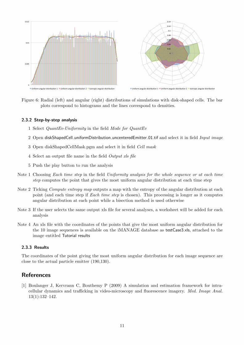
Figure 6: Radial (left) and angular (right) distributions of simulations with disk-shaped cells. The barplots correspond to histograms and the lines correspond to densities.

2.3.2 Step-by-step analysis

1 Select QuantEv-Uniformity in the field Mode for QuantEv

2 Open diskShapedCell uniformDistribution uncenteredEmitter 01.tif and select it in field Input image

3 Open diskShapedCellMask.pgm and select it in field Cell mask

4 Select an output file name in the field Output xls file

5 Push the play button to run the analysis

Note 1 Choosing Each time step in the field Uniformity analysis for the whole sequence or at each timestep computes the point that gives the most uniform angular distribution at each time step

Note 2 Ticking Compute entropy map outputs a map with the entropy of the angular distribution at eachpoint (and each time step if Each time step is chosen). This processing is longer as it computesangular distribution at each point while a bisection method is used otherwise

Note 3 If the user selects the same output xls file for several analyses, a worksheet will be added for eachanalysis

Note 4 An xls file with the coordinates of the points that give the most uniform angular distribution forthe 10 image sequences is available on the iMANAGE database as testCase3.xls, attached to theimage entitled Tutorial results

2.3.3 Results

The coordinates of the point giving the most uniform angular distribution for each image sequence areclose to the actual particle emitter (190,130).

References

[1] Boulanger J, Kervrann C, Bouthemy P (2009) A simulation and estimation framework for intra-cellular dynamics and trafficking in video-microscopy and fluorescence imagery. Med. Image Anal.13(1):132–142.

11