Embed Size (px)
Citation preview

ANSYS Fluid Dynamics Verification Manual
Release 14.5ANSYS, Inc.
October 2012Southpointe
275 Technology Drive
Canonsburg, PA 15317 ANSYS, Inc. is
certified to ISO
9001:[email protected]
http://www.ansys.com
(T) 724-746-3304
(F) 724-514-9494
Copyright and Trademark Information
© 2012 SAS IP, Inc. All rights reserved. Unauthorized use, distribution or duplication is prohibited.
ANSYS, ANSYS Workbench, Ansoft, AUTODYN, EKM, Engineering Knowledge Manager, CFX, FLUENT, HFSS and any
and all ANSYS, Inc. brand, product, service and feature names, logos and slogans are registered trademarks or
trademarks of ANSYS, Inc. or its subsidiaries in the United States or other countries. ICEM CFD is a trademark used
by ANSYS, Inc. under license. CFX is a trademark of Sony Corporation in Japan. All other brand, product, service
and feature names or trademarks are the property of their respective owners.
Disclaimer Notice
THIS ANSYS SOFTWARE PRODUCT AND PROGRAM DOCUMENTATION INCLUDE TRADE SECRETS AND ARE CONFID-
ENTIAL AND PROPRIETARY PRODUCTS OF ANSYS, INC., ITS SUBSIDIARIES, OR LICENSORS. The software products
and documentation are furnished by ANSYS, Inc., its subsidiaries, or affiliates under a software license agreement
that contains provisions concerning non-disclosure, copying, length and nature of use, compliance with exporting
laws, warranties, disclaimers, limitations of liability, and remedies, and other provisions. The software products
and documentation may be used, disclosed, transferred, or copied only in accordance with the terms and conditions
of that software license agreement.
ANSYS, Inc. is certified to ISO 9001:2008.
U.S. Government Rights
For U.S. Government users, except as specifically granted by the ANSYS, Inc. software license agreement, the use,
duplication, or disclosure by the United States Government is subject to restrictions stated in the ANSYS, Inc.
software license agreement and FAR 12.212 (for non-DOD licenses).
Third-Party Software
See the legal information in the product help files for the complete Legal Notice for ANSYS proprietary software
and third-party software. If you are unable to access the Legal Notice, please contact ANSYS, Inc.
Published in the U.S.A.

Table of Contents
I. Verification Test Case Descriptions . . . . . . . . . . . . . . . . . . . . . . . . . . . . . . . . . . . . . . . . . . . . . . . . . . . . . . . . . . . . . . . . . . . . . . . . . . . . . . . . . . . . . . . . . . . . . . . . . . . . . . . . . . 1
1. Introduction . . . . . . . . . . . . . . . . . . . . . . . . . . . . . . . . . . . . . . . . . . . . . . . . . . . . . . . . . . . . . . . . . . . . . . . . . . . . . . . . . . . . . . . . . . . . . . . . . . . . . . . . . . . . . . . . . . . . . . . . . . . . . . . . . . . . . . 3
1.1. Expected Results ... . . . . . . . . . . . . . . . . . . . . . . . . . . . . . . . . . . . . . . . . . . . . . . . . . . . . . . . . . . . . . . . . . . . . . . . . . . . . . . . . . . . . . . . . . . . . . . . . . . . . . . . . . . . . . . . . . . . . . 3
1.2. References .... . . . . . . . . . . . . . . . . . . . . . . . . . . . . . . . . . . . . . . . . . . . . . . . . . . . . . . . . . . . . . . . . . . . . . . . . . . . . . . . . . . . . . . . . . . . . . . . . . . . . . . . . . . . . . . . . . . . . . . . . . . . . . . 4
1.3. Using the Verification Manual and Test Cases .... . . . . . . . . . . . . . . . . . . . . . . . . . . . . . . . . . . . . . . . . . . . . . . . . . . . . . . . . . . . . . . . . . . . . . . . . . . . 4
1.4. Quality Assurance Services .... . . . . . . . . . . . . . . . . . . . . . . . . . . . . . . . . . . . . . . . . . . . . . . . . . . . . . . . . . . . . . . . . . . . . . . . . . . . . . . . . . . . . . . . . . . . . . . . . . . . . . . 5
1.5. Index of ANSYS Fluid Dynamics Test cases .... . . . . . . . . . . . . . . . . . . . . . . . . . . . . . . . . . . . . . . . . . . . . . . . . . . . . . . . . . . . . . . . . . . . . . . . . . . . . . . . 5
01. VMFL001: Flow Between Rotating and Stationary Concentric Cylinders .... . . . . . . . . . . . . . . . . . . . . . . . . . . . . . . . . . . . . . . . . . . . 9
02.VMFL002: Laminar Flow Through a Pipe with Uniform Heat Flux .... . . . . . . . . . . . . . . . . . . . . . . . . . . . . . . . . . . . . . . . . . . . . . . . . . . . . 11
03. VMFL003: Pressure Drop in Turbulent Flow through a Pipe .... . . . . . . . . . . . . . . . . . . . . . . . . . . . . . . . . . . . . . . . . . . . . . . . . . . . . . . . . . . . . 13
04. VMFL004: Plain Couette Flow with Pressure Gradient .... . . . . . . . . . . . . . . . . . . . . . . . . . . . . . . . . . . . . . . . . . . . . . . . . . . . . . . . . . . . . . . . . . . . . 15
05. VMFL005: Poiseuille Flow in a Pipe .... . . . . . . . . . . . . . . . . . . . . . . . . . . . . . . . . . . . . . . . . . . . . . . . . . . . . . . . . . . . . . . . . . . . . . . . . . . . . . . . . . . . . . . . . . . . . . . . . 19
06. VMFL006: Multicomponent Species Transport in Pipe Flow .... . . . . . . . . . . . . . . . . . . . . . . . . . . . . . . . . . . . . . . . . . . . . . . . . . . . . . . . . . . . 21
07. VMFL007: Non-Newtonian Flow in a Pipe .... . . . . . . . . . . . . . . . . . . . . . . . . . . . . . . . . . . . . . . . . . . . . . . . . . . . . . . . . . . . . . . . . . . . . . . . . . . . . . . . . . . . . . . 23
08. VMFL008: Flow Inside a Rotating Cavity .... . . . . . . . . . . . . . . . . . . . . . . . . . . . . . . . . . . . . . . . . . . . . . . . . . . . . . . . . . . . . . . . . . . . . . . . . . . . . . . . . . . . . . . . . 25
09. VMFL009: Natural Convection in a Concentric Annulus .... . . . . . . . . . . . . . . . . . . . . . . . . . . . . . . . . . . . . . . . . . . . . . . . . . . . . . . . . . . . . . . . . . 29
10. VMFL010: Laminar Flow in a 90° Tee-Junction. ... . . . . . . . . . . . . . . . . . . . . . . . . . . . . . . . . . . . . . . . . . . . . . . . . . . . . . . . . . . . . . . . . . . . . . . . . . . . . . . . 33
11.VMFL011: Laminar flow in a Triangular Cavity .... . . . . . . . . . . . . . . . . . . . . . . . . . . . . . . . . . . . . . . . . . . . . . . . . . . . . . . . . . . . . . . . . . . . . . . . . . . . . . . . . 37
12. VMFL012: Turbulent Flow in a Wavy Channel ... . . . . . . . . . . . . . . . . . . . . . . . . . . . . . . . . . . . . . . . . . . . . . . . . . . . . . . . . . . . . . . . . . . . . . . . . . . . . . . . . . 41
13. VMFL013: Turbulent Flow with Heat Transfer in a Backward-Facing Step .... . . . . . . . . . . . . . . . . . . . . . . . . . . . . . . . . . . . . . . . . 45
14. VMFL014: Species Mixing in Co-axial Turbulent Jets ... . . . . . . . . . . . . . . . . . . . . . . . . . . . . . . . . . . . . . . . . . . . . . . . . . . . . . . . . . . . . . . . . . . . . . . . 47
15.VMFL015: Flow Through an Engine Inlet Valve .... . . . . . . . . . . . . . . . . . . . . . . . . . . . . . . . . . . . . . . . . . . . . . . . . . . . . . . . . . . . . . . . . . . . . . . . . . . . . . . . 51
16. VMFL016: Turbulent Flow in a Transition Duct .... . . . . . . . . . . . . . . . . . . . . . . . . . . . . . . . . . . . . . . . . . . . . . . . . . . . . . . . . . . . . . . . . . . . . . . . . . . . . . . . 55
17. VMFL017: Transonic Flow over an RAE 2822 Airfoil .. . . . . . . . . . . . . . . . . . . . . . . . . . . . . . . . . . . . . . . . . . . . . . . . . . . . . . . . . . . . . . . . . . . . . . . . . . . 59
18. VMFL018: Shock Reflection in Supersonic Flow .... . . . . . . . . . . . . . . . . . . . . . . . . . . . . . . . . . . . . . . . . . . . . . . . . . . . . . . . . . . . . . . . . . . . . . . . . . . . . . 61
19. VMFL019: Transient Flow near a Wall Set in Motion .... . . . . . . . . . . . . . . . . . . . . . . . . . . . . . . . . . . . . . . . . . . . . . . . . . . . . . . . . . . . . . . . . . . . . . . . 65
20. VMFL020: Adiabatic Compression of Air in Cylinder by a Reciprocating Piston .... . . . . . . . . . . . . . . . . . . . . . . . . . . . . . . . 67
21. VMFL021: Cavitation over a Sharp-Edged Orifice Case A: High Inlet Pressure .... . . . . . . . . . . . . . . . . . . . . . . . . . . . . . . . . . . 71
22. VMFL022: Cavitation over a Sharp-Edged Orifice Case B: Low Inlet Pressure .... . . . . . . . . . . . . . . . . . . . . . . . . . . . . . . . . . . . 75
23. VMFL023: Oscillating Laminar Flow Around a Circular Cylinder .... . . . . . . . . . . . . . . . . . . . . . . . . . . . . . . . . . . . . . . . . . . . . . . . . . . . . . . 79
24. VMFL024: Interface of Two Immiscible Liquids in a Rotating Cylinder .... . . . . . . . . . . . . . . . . . . . . . . . . . . . . . . . . . . . . . . . . . . . . . 81
25.VMFL025:Turbulent Non-Premixed Methane Combustion with Swirling Air ... . . . . . . . . . . . . . . . . . . . . . . . . . . . . . . . . . . . . 83
26. VMFL026: Supersonic Flow with Real Gas Effects inside a Shock Tube .... . . . . . . . . . . . . . . . . . . . . . . . . . . . . . . . . . . . . . . . . . . . . 91
27.VMFL027:Turbulent Flow over a Backward-Facing Step .... . . . . . . . . . . . . . . . . . . . . . . . . . . . . . . . . . . . . . . . . . . . . . . . . . . . . . . . . . . . . . . . . . 95
28. VMFL028: Turbulent Heat Transfer in a Pipe Expansion .... . . . . . . . . . . . . . . . . . . . . . . . . . . . . . . . . . . . . . . . . . . . . . . . . . . . . . . . . . . . . . . . . . . 99
29. VMFL029: Anisotropic Conduction Heat Transfer ... . . . . . . . . . . . . . . . . . . . . . . . . . . . . . . . . . . . . . . . . . . . . . . . . . . . . . . . . . . . . . . . . . . . . . . . . . . 101
30. VMFL030: Turbulent Flow in a 90° Pipe-Bend .... . . . . . . . . . . . . . . . . . . . . . . . . . . . . . . . . . . . . . . . . . . . . . . . . . . . . . . . . . . . . . . . . . . . . . . . . . . . . . . . 103
31.VMFL031:Turbulent Flow Behind an Open-Slit V Gutter ... . . . . . . . . . . . . . . . . . . . . . . . . . . . . . . . . . . . . . . . . . . . . . . . . . . . . . . . . . . . . . . . . 105
32. VMFL032: Turbulent Flow with Separation Along an Axisymmetric Afterbody .... . . . . . . . . . . . . . . . . . . . . . . . . . . . . . . 109
33. VMFL033: Viscous Heating in an Annulus .... . . . . . . . . . . . . . . . . . . . . . . . . . . . . . . . . . . . . . . . . . . . . . . . . . . . . . . . . . . . . . . . . . . . . . . . . . . . . . . . . . . . . 113
34. VMFL034: Particle Aggregation inside a Turbulent Stirred Tank .... . . . . . . . . . . . . . . . . . . . . . . . . . . . . . . . . . . . . . . . . . . . . . . . . . . . . 117
35. VMFL035: 3-Dimensional Single-Stage Axial Compressor .... . . . . . . . . . . . . . . . . . . . . . . . . . . . . . . . . . . . . . . . . . . . . . . . . . . . . . . . . . . . . 119
36. VMFL036: Turbulent Round Jet ... . . . . . . . . . . . . . . . . . . . . . . . . . . . . . . . . . . . . . . . . . . . . . . . . . . . . . . . . . . . . . . . . . . . . . . . . . . . . . . . . . . . . . . . . . . . . . . . . . . . . 121
37. VMFL037: Turbulent Flow over a Forward Facing Step .... . . . . . . . . . . . . . . . . . . . . . . . . . . . . . . . . . . . . . . . . . . . . . . . . . . . . . . . . . . . . . . . . . 125
38. VMFL038: Falling Film over an Inclined Plane .... . . . . . . . . . . . . . . . . . . . . . . . . . . . . . . . . . . . . . . . . . . . . . . . . . . . . . . . . . . . . . . . . . . . . . . . . . . . . . . 129
39. VMFL039: Boiling in a Pipe with Heated Wall ... . . . . . . . . . . . . . . . . . . . . . . . . . . . . . . . . . . . . . . . . . . . . . . . . . . . . . . . . . . . . . . . . . . . . . . . . . . . . . . . . 131
40. VMFL040: Separated Turbulent Flow in Diffuser ... . . . . . . . . . . . . . . . . . . . . . . . . . . . . . . . . . . . . . . . . . . . . . . . . . . . . . . . . . . . . . . . . . . . . . . . . . . . 135
41. VMFL041: Transonic Flow Over an Airfoil .. . . . . . . . . . . . . . . . . . . . . . . . . . . . . . . . . . . . . . . . . . . . . . . . . . . . . . . . . . . . . . . . . . . . . . . . . . . . . . . . . . . . . . . . 139
42. VMFL042: Turbulent Mixing of Two Streams with Different Density .... . . . . . . . . . . . . . . . . . . . . . . . . . . . . . . . . . . . . . . . . . . . . . . 143
43. VMFL043: Laminar to Turbulent Transition of Boundary Layer over a Flat Plate .... . . . . . . . . . . . . . . . . . . . . . . . . . . . . . 147
iiiRelease 14.5 - © SAS IP, Inc. All rights reserved. - Contains proprietary and confidential information
of ANSYS, Inc. and its subsidiaries and affiliates.
44. VMFL044: Supersonic Nozzle Flow .... . . . . . . . . . . . . . . . . . . . . . . . . . . . . . . . . . . . . . . . . . . . . . . . . . . . . . . . . . . . . . . . . . . . . . . . . . . . . . . . . . . . . . . . . . . . . . . 149
45. VMFL045: Oblique Shock over an Inclined Ramp ..... . . . . . . . . . . . . . . . . . . . . . . . . . . . . . . . . . . . . . . . . . . . . . . . . . . . . . . . . . . . . . . . . . . . . . . . . 151
46. VMFL046: Supersonic Flow with Normal Shock in a Converging Diverging Nozzle .... . . . . . . . . . . . . . . . . . . . . . . . . 153
47. VMFL047: Turbulent Flow with Separation in an Asymmetric Diffuser ... . . . . . . . . . . . . . . . . . . . . . . . . . . . . . . . . . . . . . . . . . . . 155
48. VMFL048: Turbulent flow in a 180° Pipe Bend ... . . . . . . . . . . . . . . . . . . . . . . . . . . . . . . . . . . . . . . . . . . . . . . . . . . . . . . . . . . . . . . . . . . . . . . . . . . . . . . 157
49. VMFL049: Combustion in an Axisymmetric Natural Gas Furnace .... . . . . . . . . . . . . . . . . . . . . . . . . . . . . . . . . . . . . . . . . . . . . . . . . . . 161
50.VMFL050:Transient Heat Conduction in a Semi-Infinite Slab .... . . . . . . . . . . . . . . . . . . . . . . . . . . . . . . . . . . . . . . . . . . . . . . . . . . . . . . . . 165
51. VMFL051: Isentropic Expansion of Supersonic Flow over a Convex Corner .... . . . . . . . . . . . . . . . . . . . . . . . . . . . . . . . . . . . 167
52. VMFL052: Turbulent Natural Convection inside a Tall Cavity .... . . . . . . . . . . . . . . . . . . . . . . . . . . . . . . . . . . . . . . . . . . . . . . . . . . . . . . . . . 169
38. VMFL053: Compressible Turbulent Mixing Layer .... . . . . . . . . . . . . . . . . . . . . . . . . . . . . . . . . . . . . . . . . . . . . . . . . . . . . . . . . . . . . . . . . . . . . . . . . . 173
38. VMFL054: Laminar flow in a Trapezoidal Cavity .... . . . . . . . . . . . . . . . . . . . . . . . . . . . . . . . . . . . . . . . . . . . . . . . . . . . . . . . . . . . . . . . . . . . . . . . . . . . 175
55. VMFL055: Transitional Recirculatory Flow inside a Ventilation Enclosure .... . . . . . . . . . . . . . . . . . . . . . . . . . . . . . . . . . . . . . . 179
56. VMFL056: Combined Conduction and Radiation in a Square Cavity .... . . . . . . . . . . . . . . . . . . . . . . . . . . . . . . . . . . . . . . . . . . . . . 181
57. VMFL057: Radiation and Conduction in Composite Solid Layers ... . . . . . . . . . . . . . . . . . . . . . . . . . . . . . . . . . . . . . . . . . . . . . . . . . . . 183
58.VMFL058:Turbulent Flow in an Axisymmetric Diffuser ... . . . . . . . . . . . . . . . . . . . . . . . . . . . . . . . . . . . . . . . . . . . . . . . . . . . . . . . . . . . . . . . . . . 185
59. VMFL059: Conduction in a Composite Solid Block ... . . . . . . . . . . . . . . . . . . . . . . . . . . . . . . . . . . . . . . . . . . . . . . . . . . . . . . . . . . . . . . . . . . . . . . . 187
60. VMFL060: Transitional Supersonic Flow over a Rearward Facing Step .... . . . . . . . . . . . . . . . . . . . . . . . . . . . . . . . . . . . . . . . . . . . 189
61. VMFL061: Surface to Surface Radiative Heat Transfer between Two Concentric Cylinders ... . . . . . . . . . . . . . 191
62. VMFL062: Fully Developed Turbulent Flow Over a “Hill” ... . . . . . . . . . . . . . . . . . . . . . . . . . . . . . . . . . . . . . . . . . . . . . . . . . . . . . . . . . . . . . . . . 195
63. VMFL063: Separated Laminar Flow over a Blunt Plate .... . . . . . . . . . . . . . . . . . . . . . . . . . . . . . . . . . . . . . . . . . . . . . . . . . . . . . . . . . . . . . . . . . . 197
64. VMFL064: Low Reynolds Number Flow in a Channel with Sudden Asymmetric Expansion .... . . . . . . . . . . . . 199
65. VMFL065: Swirling Turbulent Flow Inside a Diffuser ... . . . . . . . . . . . . . . . . . . . . . . . . . . . . . . . . . . . . . . . . . . . . . . . . . . . . . . . . . . . . . . . . . . . . . . 201
66.VMFL066: Radiative Heat Transfer in a Rectangular Enclosure with Participating Medium ..... . . . . . . . . . . . . 203
67. VMFL067: Boiling in a Pipe-Critical Heat Flux ... . . . . . . . . . . . . . . . . . . . . . . . . . . . . . . . . . . . . . . . . . . . . . . . . . . . . . . . . . . . . . . . . . . . . . . . . . . . . . . . 205
68. VMFL068: Axial Flow in an Eccentric Annulus ... . . . . . . . . . . . . . . . . . . . . . . . . . . . . . . . . . . . . . . . . . . . . . . . . . . . . . . . . . . . . . . . . . . . . . . . . . . . . . . 207
69. VMFL069: Two Phase Poiseulle Flow ... . . . . . . . . . . . . . . . . . . . . . . . . . . . . . . . . . . . . . . . . . . . . . . . . . . . . . . . . . . . . . . . . . . . . . . . . . . . . . . . . . . . . . . . . . . . . 209
70. VMFL070: Radiation Between Two Parallel Surfaces .... . . . . . . . . . . . . . . . . . . . . . . . . . . . . . . . . . . . . . . . . . . . . . . . . . . . . . . . . . . . . . . . . . . . . . 211
Release 14.5 - © SAS IP, Inc. All rights reserved. - Contains proprietary and confidential informationof ANSYS, Inc. and its subsidiaries and affiliates.iv
Fluid Dynamics Verification Manual

Part I: Verification Test Case Descriptions


Chapter 1: Introduction
The Fluid Dynamics Verification Manual presents a collection of test cases that demonstrate a represent-
ative set of the capabilities of the ANSYS Fluid Dynamics product suite. The primary purpose of this
manual is to demonstrate a wide range of capabilities in straightforward problems that have "classical"
or readily-obtainable theoretical solutions and in some cases have experimental data for comparison.
The close agreement of the ANSYS solutions to the theoretical or experimental results in this manual
is intended to provide user confidence in the ANSYS solutions. These problems may then serve as the
basis for your additional validation and qualification of ANSYS capabilities for specific applications that
may be of interest to you.
This manual represents a small subset of the Quality Assurance test case library that is used in full when
testing new versions of ANSYS FLUENT and ANSYS CFX. This test library and the test cases in this
manual represent comparisons of ANSYS solutions with known theoretical solutions, experimental results,
or other independently calculated solutions. Because ANSYS FLUENT and ANSYS CFX are programs
capable of solving very complicated practical engineering problems having no closed-form theoretical
solutions, the relatively simple problems solved in this manual do not illustrate the full capability of
these ANSYS programs.
The ANSYS software suite is continually being verified by the developers at ANSYS as new capabilities
are added to the software. Verification of ANSYS products is conducted in accordance with written
procedures that form a part of an overall Quality Assurance program at ANSYS, Inc.
Note
In order to solve test cases, you will require product licenses: ANSYS CFD, ANSYS FLUENT,
or ANSYS CFX.
1.1. Expected Results
The test cases in this manual have been modeled to give reasonably accurate comparisons with a low
number of elements and iterations. In some cases, even fewer elements and/or iterations will still yield
an acceptable accuracy. The test cases employ a balance between accuracy and solution time. An attempt
has been made to present a test case and results that are grid-independent. If test results are not grid-
independent, it is due to the need to limit the run time for the test to be in the manual. Improved results
can be obtained in some cases by refining the mesh, but this requires longer solution times.
The ANSYS solutions in this manual are compared with solutions or experimental data from textbooks
or technical publications. In some cases, the target (theoretical) answers reported in this manual may
differ from those shown in the reference. In several fluid flow simulation problems where experimental
results are available in the form of plots of the relevant parameters, the simulation results are also
presented as plots so that the corresponding values can be compared on the same graph.
Many of the fluid-dynamics simulation methods have to make use of data available from experimental
measurements for their verification primarily because closed-form theoretical solutions are not available
for modeling the related phenomena. In this manual several test cases for ANSYS FLUENT and ANSYS
3Release 14.5 - © SAS IP, Inc. All rights reserved. - Contains proprietary and confidential information
of ANSYS, Inc. and its subsidiaries and affiliates.

CFX make use of experimental data published in reputed journals or conference proceedings for verific-
ation of the computational results. The experimental measurements for fluid-flow systems are often
presented in the form of plots of the relevant parameters. Hence the published experimental data for
those cases and the corresponding simulation results are presented in graphical format to facilitate
comparison.
Experimental data represent the "real world" physics reproduced in a controlled manner and provides
more complex details of the flow field than theoretical solutions. The test cases in this manual have
been modeled to give reasonably accurate comparisons with experimental data wherever applicable,
with a low number of elements and iterations.
Different computers and operating systems may yield slightly different results for some of the test cases
in this manual due to numerical precision variation from machine to machine. Solutions that are non-
linear, iterative, or have convergence options activated are among the most likely to exhibit machine-
dependent numerical differences. Because of this, an effort has been made to report an appropriate
and consistent number of significant digits in both the target and the ANSYS solution. If you run these
test cases on your own computer hardware, be advised that an ANSYS result reported in this manual
as 0.01234 may very well show up in your printout as 0.012335271.
1.2. References
The goal for the test cases contained in this manual was to have results accuracy within 3% of the target
solution. The solutions for the test cases have been verified; however, certain differences may exist with
regard to the references. These differences have been examined and are considered acceptable.
It should be noted that only those items corresponding to the given theoretical solution values are re-
ported for each problem. In most cases the same solution also contains a considerable amount of other
useful numerical solution data.
Different computers and different operating systems may yield slightly different results for some of the
test cases in this manual, since numerical precision varies from machine to machine. Because of this,
an effort has been made to report an appropriate and consistent number of significant digits in both
the target and the ANSYS solution. These results reported in this manual are from runs on an Intel Xeon
processor using Microsoft Windows XP Professional. Slightly different results may be obtained when
different processor types or operating systems are used.
1.3. Using the Verification Manual and Test Cases
You are encouraged to use these tests as starting points when exploring features in these products.
Geometries, material properties, loads, and output results can easily be changed and the solution re-
peated. As a result, the tests offer a quick introduction to new features with which you may be unfamil-
iar.
The test cases in this manual are primarily intended for verification of the ANSYS programs. An attempt
has been made to include most significant analysis capabilities of the ANSYS products in this manual.
Although they are valuable as demonstration problems, the test cases are not presented as step-by-
step examples with lengthy data input instructions and printouts. The reader should refer to the online
help for complete input data instructions.
Users desiring more detailed instructions for solving problems or in-depth treatment of specific topics
should refer to the ANSYS FLUENT documentation. ANSYS FLUENT tutorials and ANSYS CFX tutorials
are also available for various specific topics. These publications focus on particular features or program
Release 14.5 - © SAS IP, Inc. All rights reserved. - Contains proprietary and confidential informationof ANSYS, Inc. and its subsidiaries and affiliates.4
Introduction

areas, supplementing other ANSYS reference documents with theory, procedures, guidelines, examples,
and references.
1.4. Quality Assurance Services
For customers who may have further need for formal verification of the ANSYS products on their com-
puters, ANSYS, Inc. offers the Quality Assurance Testing Agreement. You are provided with input data,
output data, comparator software, and software tools for automating the testing and reporting process.
If you are interested in contracting for such services, contact the ANSYS, Inc. Quality Assurance Group.
1.5. Index of ANSYS Fluid Dynamics Test cases
Dimensionality Column Key:
• 2: 2D
• 3: 3D
• A: 2D Axisymmetric
2VMFL001
XAVMFL002
XAVMFL003
2VMFL004
AVMFL005
XAVMFL006
AVMFL007
XAVMFL008
XX2VMFL009
2VMFL010
2VMFL011
X2VMFL012
XX2VMFL013
XXAVMFL014
X3VMFL015
X3VMFL016
XXX2VMFL017
XXX2VMFL018
X2VMFL019
XXX2VMFL020
5Release 14.5 - © SAS IP, Inc. All rights reserved. - Contains proprietary and confidential information
of ANSYS, Inc. and its subsidiaries and affiliates.
Index of ANSYS Fluid Dynamics Test cases

XXXAVMFL021
XXXAVMFL022
X2VMFL023
XXXAVMFL024
XXXXAVMFL025
XXXX3VMFL026
X2VMFL027
XXAVMFL028
XX2VMFL029
X3VMFL030
X2VMFL031
XAVMFL032
X2VMFL033
XX2VMFL034
XXXX3VMFL035
XAVMFL036
X2VMFL037
XX2VMFL038
XXXXXAVMFL039
XAVMFL040
XXX2VMFL041
XXX2VMFL042
XX2VMFL043
XXXAVMFL044
XX2VMFL045
XXX2VMFL046
X2VMFL047
X3VMFL048
XXXXAVMFL049
XX2VMFL050
XXX2VMFL051
XX2VMFL052
XXX2VMFL053
2VMFL054
Release 14.5 - © SAS IP, Inc. All rights reserved. - Contains proprietary and confidential informationof ANSYS, Inc. and its subsidiaries and affiliates.6
Introduction

XXX2VMFL055
XX2VMFL056
XX2VMFL057
XAVMFL058
X2VMFL059
XXXX2VMFL060
XX2VMFL061
X2VMFL062
2VMFL063
2VMFL064
XAVMFL065
XX2VMFL066
7Release 14.5 - © SAS IP, Inc. All rights reserved. - Contains proprietary and confidential information
of ANSYS, Inc. and its subsidiaries and affiliates.
Index of ANSYS Fluid Dynamics Test cases

Release 14.5 - © SAS IP, Inc. All rights reserved. - Contains proprietary and confidential informationof ANSYS, Inc. and its subsidiaries and affiliates.8

VMFL001: Flow Between Rotating and Stationary Concentric Cylinders
Overview
F. M. White. “Viscous Fluid Flow”. Section 3-2.3. McGraw-Hill Book Co., Inc.. New
York, NY. 1991.
Reference
ANSYS FLUENT, ANSYS CFXSolver
Laminar flow, rotating wallPhysics/Models
rot_conc_cyl.cas for ANSYS FLUENTInput Files
rotating_cylinder.def for ANSYS CFX
Test Case
Steady laminar flow between two concentric cylinders is modeled. The flow is induced by rotation of
the inner cylinder with a constant angular velocity, while the outer cylinder is held stationary. Due to
periodicity only a section of the domain needs to be modeled. In the present simulation a 180° segment
(half of the domain shown in Figure 01.1: Flow Domain (p. 9)) is modeled. The sketch is not to scale.
Figure 01.1: Flow Domain
Inner Cylinder
Outer Cylinder
r2
r1x
y
Boundary ConditionsGeometryMaterial Properties
Angular velocity of the inner wall
= 1 rad/s
Radius of the Inner Cylinder =
17.8 mmDensity = 1 kg/m
3
Viscosity = 0.0002
kg/m-s Radius of the outer Cylinder =
46.8 mm
Analysis Assumptions and Modeling Notes
The flow is steady. The tangential velocity at various sections can be calculated using analytical equations
for laminar flow. These values are used for comparison with simulation results.
9Release 14.5 - © SAS IP, Inc. All rights reserved. - Contains proprietary and confidential information
of ANSYS, Inc. and its subsidiaries and affiliates.

Results Comparison for ANSYS FLUENT
Table 01.1: Comparison of Tangential Velocity in the Annulus at Various Radial Locations
RatioANSYS FLUENT, m/sTarget Calculation, m/sTangential Velocity at
0.9990.01510.0151r = 20 mm
0.9960.01050.0105r = 25 mm
0.9900.00720.0072r = 30 mm
0.9790.00450.0046r = 35 mm
Results Comparison for ANSYS CFX
Table 01.2: Comparison of Tangential Velocity in the Annulus at Various Radial Locations
RatioANSYS CFX, m/sTarget Calculation, m/sLocation
0.9910.01500.0151r = 20 mm
0.9980.01050.0105r = 25 mm
0.9880.00710.0072r = 30 mm
0.9760.00450.0046r = 35 mm
Release 14.5 - © SAS IP, Inc. All rights reserved. - Contains proprietary and confidential informationof ANSYS, Inc. and its subsidiaries and affiliates.10
VMFL001

VMFL002: Laminar Flow Through a Pipe with Uniform Heat Flux
Overview
Reference F. M. White. “Fluid Mechanics ”. 3rd Edition. McGraw-Hill Book Co.. New
York, NY. 1994.
F. P. Incropera and D. P. DeWitt. “Fundamentals of Heat Transfer”. John
Wiley & Sons. 1981.
ANSYS FLUENT, ANSYS CFXSolver
Laminar flow with heat transferPhysics/Models
Input File laminar-pipe-hotflow.cas for ANSYS FLUENT
VMFL002B_VV002CFX.def for ANSYS CFX
Test Case
Laminar flow of Mercury through a circular pipe is modeled, with uniform heat flux across the wall. A
fully developed laminar velocity profile is prescribed at the inlet. The resulting pressure drop and exit
temperature are compared with analytical calculations for Laminar flow. Only half of the 2–D domain
is modeled due to symmetry.
Figure 02.1: Flow Domain
r
r = R w
(r)
Pi
τ
τ
V (r)
Po
x
Boundary ConditionsGeometryMaterial Properties
Fully developed velocity profile at
inlet.
Length of the pipe = 0.1 m
Radius of the pipe = 0.0025
m
Fluid: Mercury
Density = 13529
kg/m3 Inlet temperature = 300 K
Heat Flux across wall = 5000 W/m2
Viscosity = 0.001523
kg/m-s
Specific Heat = 139.3
J/kg-K
Thermal Conductivity
= 8.54 W/m-K
Analysis Assumptions and Modeling Notes
The flow is steady and incompressible. Pressure drop can be calculated from the theoretical expression
for laminar flow given in Ref. 1. Correlations for temperature calculations are given in Ref. 2.
11Release 14.5 - © SAS IP, Inc. All rights reserved. - Contains proprietary and confidential information
of ANSYS, Inc. and its subsidiaries and affiliates.

Results Comparison for ANSYS FLUENT
Table 02.1: Comparison of Pressure Drop and Outlet Temperature
RatioANSYS FLUENTTarget Calculation
0.9990.999 Pa1.000 PaPressure Drop
0.999340.50 K341.00 KCenterline Temperature
at the Outlet
Results Comparison for ANSYS CFX
Table 02.2: Comparison of Pressure Drop and Outlet Temperature
RatioANSYS CFXTarget Calculation
1.0191.019 Pa1.000 PaPressure Drop
0.9994340.8 K341.00 KCenterline Temperature
at the Outlet
Release 14.5 - © SAS IP, Inc. All rights reserved. - Contains proprietary and confidential informationof ANSYS, Inc. and its subsidiaries and affiliates.12
VMFL002

VMFL003: Pressure Drop in Turbulent Flow through a Pipe
Overview
F. M. White. “Fluid Mechanics”. 3rd Edition. McGraw-Hill Co.. New York, NY. 1994.Reference
ANSYS FLUENT, ANSYS CFXSolver
Turbulent flow, standard k-ε ModelPhysics/Models
Input File turb_pipe_flow.cas for ANSYS FLUENT
VMFL003B_VV003CFX.def for ANSYS CFX
Test Case
Air flows through a horizontal pipe with smooth walls. The flow Reynolds number is 1.37 X 10⁴. Only
half of the axisymmetrical domain is modeled.
Figure 03.1: Flow Domain
ℓ
P1
v
Inlet Outlet
P2
The figure is not to scale.
Boundary ConditionsGeometryMaterial Properties
Inlet velocity = 50 m/sLength of the pipe =
2 mDensity = 1.225 kg/m
3
Viscosity = 1.7894 X 10⁻⁵
kg/m-sOutlet pressure = 0 Pa
Radius of the pipe =
0.002 m
Analysis Assumptions and Modeling Notes
The flow is steady. Pressure drop can be calculated from analytical formula using friction factor f which
can be determined for the given Reynolds number from Moody chart. The calculated pressure drop is
compared with the simulation results (pressure difference between inlet and outlet).
Results Comparison for ANSYS FLUENT
Table 03.1: Comparison of Pressure Drop in the Pipe
RatioANSYS FLUENTTarget Calculation
0.98821480 Pa21789 PaPressure Drop
13Release 14.5 - © SAS IP, Inc. All rights reserved. - Contains proprietary and confidential information
of ANSYS, Inc. and its subsidiaries and affiliates.

Results Comparison for ANSYS CFX
Table 03.2: Comparison of Pressure Drop in the Pipe
RatioANSYS CFXTarget Calculation
0.997521740 Pa21789 PaPressure Drop
Release 14.5 - © SAS IP, Inc. All rights reserved. - Contains proprietary and confidential informationof ANSYS, Inc. and its subsidiaries and affiliates.14
VMFL003

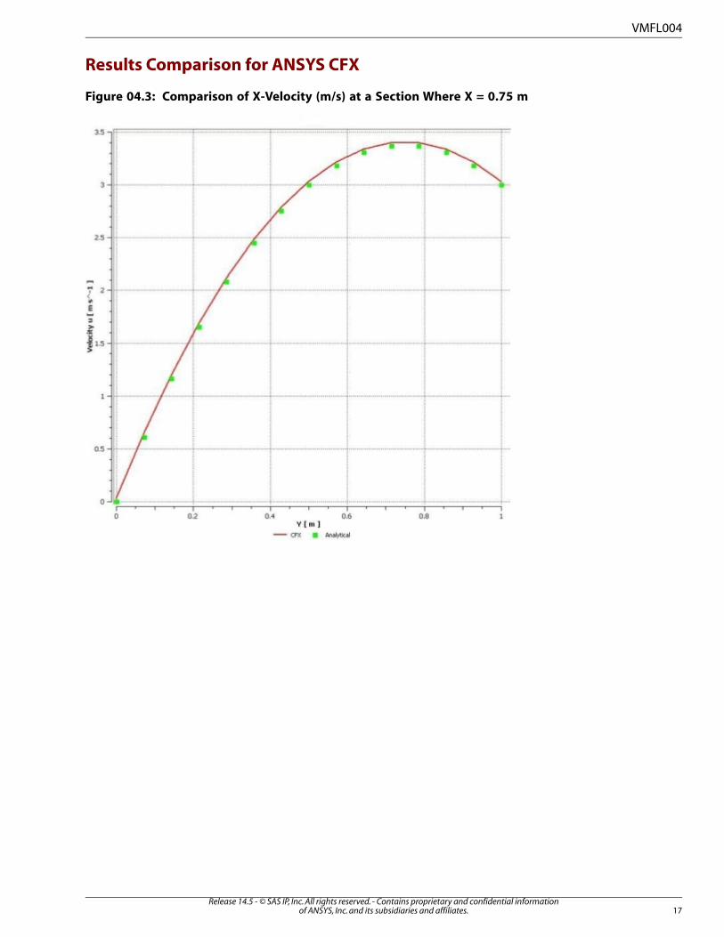
VMFL004: Plain Couette Flow with Pressure Gradient
Overview
Munon, Young, Okiishi. “Fundamentals of Fluid Mechanics”. 5th Edition.Reference
ANSYS FLUENT, ANSYS CFXSolver
Laminar flow, moving wall, periodic boundariesPhysics/Models
Input Files couette_flow.cas for ANSYS FLUENT
Couette_Flow.def for ANSYS CFX
Test Case
Viscous flow between two parallel plates is modeled. The top plate moves with a uniform velocity while
the lower plate is fixed. A pressure gradient is imposed in a direction parallel to the plates.
Figure 04.1: Flow Domain
Moving Wall
Periodic Boundaries
Stationary Wall
Boundary ConditionsGeometryMaterial Properties
Velocity of the moving wall = 3
m/s in X-direction
Length of the domain =
1.5 mDensity = 1 kg/m
3
Viscosity = 1 kg/m-sFor ANSYS FLUENT, pressure
gradient across periodic
boundaries = -12 Pa/m
Width of the domain = 1
m
For ANSYS CFX, pressure gradi-
ent across periodic boundaries
= -12 Pa/m (pressure change =
–18 Pa)
Analysis Assumptions and Modeling Notes
The flow is steady and laminar. Periodic conditions with specified pressure drop are applied across the
flux boundaries.
15Release 14.5 - © SAS IP, Inc. All rights reserved. - Contains proprietary and confidential information
of ANSYS, Inc. and its subsidiaries and affiliates.

Results Comparison for ANSYS FLUENT
Figure 04.2: Comparison of X-Velocity (m/s) at a Section Where X = 0.75 m
Release 14.5 - © SAS IP, Inc. All rights reserved. - Contains proprietary and confidential informationof ANSYS, Inc. and its subsidiaries and affiliates.16
VMFL004
Results Comparison for ANSYS CFX
Figure 04.3: Comparison of X-Velocity (m/s) at a Section Where X = 0.75 m
17Release 14.5 - © SAS IP, Inc. All rights reserved. - Contains proprietary and confidential information
of ANSYS, Inc. and its subsidiaries and affiliates.
VMFL004

Release 14.5 - © SAS IP, Inc. All rights reserved. - Contains proprietary and confidential informationof ANSYS, Inc. and its subsidiaries and affiliates.18

VMFL005: Poiseuille Flow in a Pipe
Overview
F. M. White. “Fluid Mechanics”. 3rd Edition. McGraw-Hill Book Co.. New York, NY.
1994.
Reference
ANSYS FLUENT, ANSYS CFXSolver
Steady laminar flowPhysics/Models
Input File poiseuille-flow.cas for ANSYS FLUENT
VMFL005B_VV005CFX.def for ANSYS CFX
Test Case
Fully developed laminar flow in a circular tube is modeled. Reynolds number based on the tube diameter
is 500. Only half of the axisymmetric domain is modeled.
Figure 05.1: Flow Domain
Inlet AxisPipe Wall
Outlet
Boundary ConditionsGeometryMaterial Properties
Fully developed laminar velocity
profile at inlet with an average ve-
locity of 2.00 m/s
Length of the pipe = 0.1
m
Radius of the pipe =
0.00125 m
Density = 1 kg/m3
Viscosity = 1e-5 kg/m-s
Analysis Assumptions and Modeling Notes
The flow is steady. A fully developed laminar velocity profile is prescribed at the inlet. Hagen-Poiseuille
equation is used to determine the pressure drop analytically.
Results Comparison for ANSYS FLUENT
Table 05.1: Comparison of Pressure Drop in the Pipe
Ra-
tio
ANSYS FLU-
ENT
Target Calcula-
tion
0.99810.22 Pa10. 24 PaPressure
Drop
19Release 14.5 - © SAS IP, Inc. All rights reserved. - Contains proprietary and confidential information
of ANSYS, Inc. and its subsidiaries and affiliates.

Results Comparison for ANSYS CFX
Table 05.2: Comparison of Pressure Drop in the Pipe
Ra-
tio
ANSYS
CFX
Target Calcula-
tion
1.02410.49 Pa10. 24 PaPressure
Drop
Release 14.5 - © SAS IP, Inc. All rights reserved. - Contains proprietary and confidential informationof ANSYS, Inc. and its subsidiaries and affiliates.20
VMFL005

VMFL006: Multicomponent Species Transport in Pipe Flow
Overview
W. M. Kays and M. E. Crawford. “Convective Heat and Mass Transfer”. 3rd Edition.
McGraw-Hill Book Co., Inc.. New York, NY. 126-134. 1993.
Reference
ANSYS FLUENT (ANSYS CFX simulation is not available for this case)Solver
Steady laminar flow, species transportPhysics/Models
Species-diffusion.casInput File
Test Case
Fully developed laminar flow in a circular tube, with two species is modeled. Species A enters at the
inlet and species B enters from the wall. Uniform and dissimilar mass fractions are specified at the pipe
inlet and wall. Fluid properties are assumed to be the same for both species, so that computed results
can be compared with analytical solution.
Figure 06.1: Flow Domain
Inlet AxisPipe Wall
Outlet
Boundary ConditionsGeometryMaterial Properties
Fully developed laminar velocity
profile at inlet with an average
velocity of 1 m/s
Length of the pipe = 0.1
m
Radius of the pipe =
0.0025 m
Species A
Density = 1 kg/m3
Viscosity = 1.0 x 10⁻⁵
Pa-s Mass fraction of species A at pipe
inlet = 1.0
Diffusivity BA = 1.43 x 10⁻⁵
m2/s
Mass fraction of species B at pipe
inlet = 0.0
Mass fraction of species A at pipe
wall = 0.0
Species B
Density = 1 kg/m3
Mass fraction of species B at pipe
wall = 1.0Viscosity = 1.0 x 10⁻⁵
Pa-s
Diffusivity AB = 1.43 x 10⁻⁵
m2/s
Analysis Assumptions and Modeling Notes
The flow is steady. A fully developed laminar velocity profile is prescribed at the inlet. Species transport
model is used.
21Release 14.5 - © SAS IP, Inc. All rights reserved. - Contains proprietary and confidential information
of ANSYS, Inc. and its subsidiaries and affiliates.

Results Comparison
Table 06.1: Comparison of Mass Fraction of Species A Along the Axis
Ra-
tio
ANSYS FLU-
ENT
Target Calcula-
tion
Axial location
(m)
1.0000.82230.82250.01
1.0000.73070.73080.02
1.0000.65920.65930.03
1.0000.59910.59920.04
1.0000.54690.54690.05
1.0000.50060.50060.06
1.0000.45910.45890.07
1.0000.42140.42120.08
1.0010.38710.38690.09
1.0010.35580.35550.10
Release 14.5 - © SAS IP, Inc. All rights reserved. - Contains proprietary and confidential informationof ANSYS, Inc. and its subsidiaries and affiliates.22
VMFL006

VMFL007: Non-Newtonian Flow in a Pipe
Overview
W. F. Hughes and J. A. Brighton. “Schaum's Outline of Theory and Problems of Fluid
Dynamics.” McGraw-Hill Book Co., Inc.. New York, NY. 1991.
Reference
ANSYS FLUENT, ANSYS CFXSolver
Steady laminar flow, power law for viscosityPhysics/Models
Input File powerlaw-visc.cas for ANSYS FLUENT
VMFL007B_vv007CFX.def for ANSYS CFX
Test Case
Flow of a non-Newtonian fluid in a circular pipe is modeled. Viscosity is specified by power law equation.
Figure 07.1: Flow Domain
Inlet AxisPipe Wall
Outlet
Boundary ConditionsGeometryMaterial Properties
Fully developed velocity profile at
inlet with an average velocity of 2
m/s
Pipe length = 0.1 m
Pipe diameter = 0.0025 m
Density = 1000 kg/m3
Viscosity: Power law
Parameters:
k = 10
n = 0.4
Analysis Assumptions and Modeling Notes
The flow is steady. Viscosity is specified using non-Newtonian power law equation.
Results Comparison for ANSYS FLUENT
Table 07.1: Comparison of Pressure Drop in the Pipe
Ra-
tio
ANSYS FLU-
ENT
Target Calcula-
tion
0.99860.37 kPa60.52 kPaPressure
Drop
23Release 14.5 - © SAS IP, Inc. All rights reserved. - Contains proprietary and confidential information
of ANSYS, Inc. and its subsidiaries and affiliates.

Results Comparison for ANSYS CFX
Table 07.2: Comparison of Pressure Drop in the Pipe
Ra-
tio
ANSYS
CFX
Target Calcula-
tion
1.016561.52 kPa60.52 kPaPressure
Drop
Release 14.5 - © SAS IP, Inc. All rights reserved. - Contains proprietary and confidential informationof ANSYS, Inc. and its subsidiaries and affiliates.24
VMFL007

VMFL008: Flow Inside a Rotating Cavity
Overview
J. A. Michelsen. “Modeling of Laminar Incompressible Rotating Fluid Flow”. AFM 86-
05., Ph.D. thesis. Department of Fluid Mechanics, Technical University of Denmark.
1986.
Reference
ANSYS FLUENT, ANSYS CFXSolver
Laminar flow, Rotating reference framePhysics/Models
Input File rotcv_RRF.cas for ANSYS FLUENT
VMFL008B_rot_cyl.def for ANSYS CFX
Test Case
Flow in a cylindrical cavity enclosed with a lid that spins at Ω = 1.0 rad/s. The flow field is 2–D
axisymmetric, so only the region bounded by the dashed lines in Figure 08.1: Flow Domain (p. 25)needs
to be modeled. The Reynolds number of the flow based on the cavity radius R and the tip-speed of the
disk is 1800.
Figure 08.1: Flow Domain
Ω
Ω
x
yR
Rotating Cover
L = 1.0 mR = 1.0 m
= 1.0 rad/s Region to
be modeledL
Boundary ConditionsGeometryMaterial Properties
Speed of rotation of the moving
wall = 1rad/s
Height of the cavity = 1m
Radius of cavity = 1m
Density = 1 kg/m3
Viscosity: 0.000556 kg/m-
s Rotational velocity for cell zone =
-1rad/s
Analysis Assumptions and Modeling Notes
The flow is laminar. The problem is solved using rotating reference frame.
25Release 14.5 - © SAS IP, Inc. All rights reserved. - Contains proprietary and confidential information
of ANSYS, Inc. and its subsidiaries and affiliates.

Results Comparison for ANSYS FLUENT
Figure 08.2: Comparison of Distribution of Radial Velocity Along a Section at X= 0.6 m
Release 14.5 - © SAS IP, Inc. All rights reserved. - Contains proprietary and confidential informationof ANSYS, Inc. and its subsidiaries and affiliates.26
VMFL008

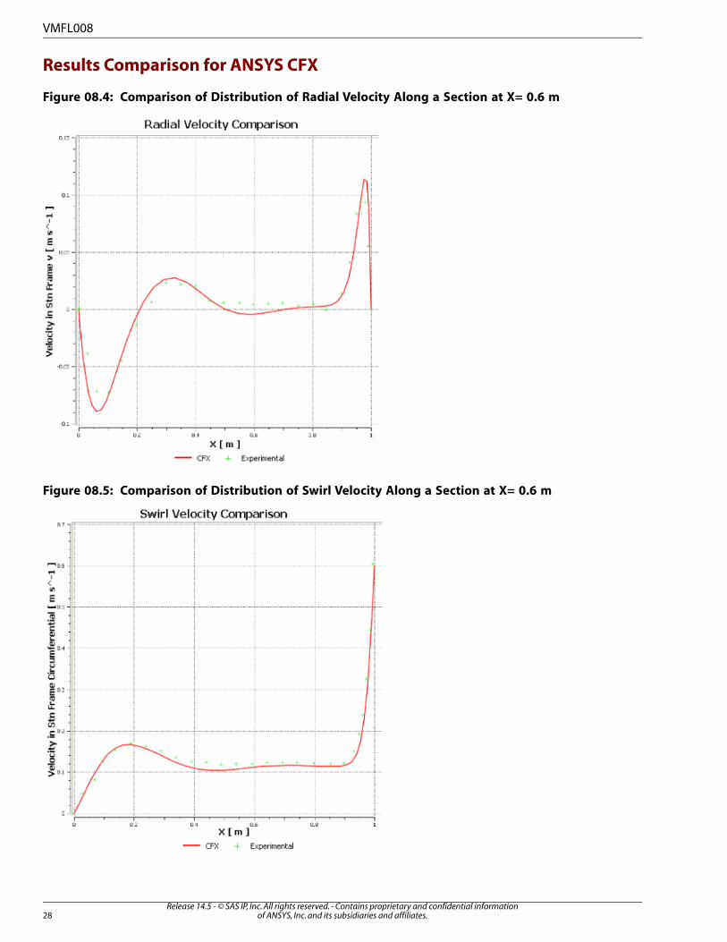
Figure 08.3: Comparison of Distribution of Swirl Velocity Along a Section at X= 0.6 m
27Release 14.5 - © SAS IP, Inc. All rights reserved. - Contains proprietary and confidential information
of ANSYS, Inc. and its subsidiaries and affiliates.
VMFL008
Results Comparison for ANSYS CFX
Figure 08.4: Comparison of Distribution of Radial Velocity Along a Section at X= 0.6 m
Figure 08.5: Comparison of Distribution of Swirl Velocity Along a Section at X= 0.6 m
Release 14.5 - © SAS IP, Inc. All rights reserved. - Contains proprietary and confidential informationof ANSYS, Inc. and its subsidiaries and affiliates.28
VMFL008

VMFL009: Natural Convection in a Concentric Annulus
Overview
Kuehn, T.H. and Goldstein, R.J., An Experimental Study of Natural Convection Heat
Transfer in Concentric and Eccentric Horizontal Cylindrical Annuli, Journal of Heat
Transfer, 100:635-640, 1978.
Reference
ANSYS FLUENT, ANSYS CFXSolver
Heat transfer, natural convection, laminar flowPhysics/Models
concn.cas for ANSYS FLUENTInput Files
ecc_cfx.def for ANSYS CFX
Test Case
Natural convection inside a concentric annular domain. The inner wall is maintained at a higher temper-
ature than the outer wall, thereby causing buoyancy induced circulation.
Figure 09.1: Flow Domain
Top Plane of Symmetry
Bottom Plane of Symmetry
Only half of the domain is modeled due to symmetry.
Boundary ConditionsGeometryMaterial Properties
Inner wall temperature = 373 KRadius of outer cylinder =
46.25 mm
Density: Incompressible
ideal gasOuter wall temperature = 327 K
Radius of inner cylinder =
17.8 mmViscosity: 2.081 X 10
-5
kg/m-s
Specific Heat: 1008 J/kg-K
29Release 14.5 - © SAS IP, Inc. All rights reserved. - Contains proprietary and confidential information
of ANSYS, Inc. and its subsidiaries and affiliates.

Boundary ConditionsGeometryMaterial Properties
Thermal Conductivity:
0.02967 W/m-K
Analysis Assumptions and Modeling Notes
The flow is symmetric and only half of the domain is modeled. Density is calculated based on incom-
pressible ideal gas assumption. The flow is laminar.
Results Comparison for ANSYS FLUENT
Figure 09.2: Comparison of Static Temperature Distribution on the Bottom Wall of Symmetry
Release 14.5 - © SAS IP, Inc. All rights reserved. - Contains proprietary and confidential informationof ANSYS, Inc. and its subsidiaries and affiliates.30
VMFL009

Figure 09.3: Comparison of Static Temperature Distribution on the Top Wall of Symmetry
31Release 14.5 - © SAS IP, Inc. All rights reserved. - Contains proprietary and confidential information
of ANSYS, Inc. and its subsidiaries and affiliates.
VMFL009

Results Comparison for ANSYS CFX
Figure 09.4: Comparison of Static Temperature Distribution on the Bottom Wall of Symmetry
Release 14.5 - © SAS IP, Inc. All rights reserved. - Contains proprietary and confidential informationof ANSYS, Inc. and its subsidiaries and affiliates.32
VMFL009

VMFL010: Laminar Flow in a 90° Tee-Junction.
Overview
R.E. Hayes, K. Nandkumar, and H. Nasr-El-Din. “Steady Laminar Flow in a 90 Degree
Planar Branch”. Computers and Fluids, 17(4). 537-553. 1989.
Reference
ANSYS FLUENT, ANSYS CFXSolver
Laminar flowPhysics/Models
Input File plarb_r4.cas for ANSYS FLUENT
VMFL010B_plarb.def for ANSYS CFX
Test Case
The purpose of this test is to compare prediction of the fractional flow in a dividing tee-junction with
experimental results. The fluid enters through the bottom branch and divides into the two channels
whose exit planes are held at the same static pressure.
33Release 14.5 - © SAS IP, Inc. All rights reserved. - Contains proprietary and confidential information
of ANSYS, Inc. and its subsidiaries and affiliates.

Figure 10.1: Flow Domain
L
L
w 2/3 L
v
w P = 0s
P = 0s
Table 10.1: Comparison of Flow Split from Tee
Boundary ConditionsGeo-
metry
Material Properties
Fully developed inlet velocity profile for: = =
where is the inlet centerline velocity.
L=3.0
m
W=1.0
m
Fluid: Air
Density : 1 kg/m3
Viscosity: 0.003333
kg/m-s=
Analysis Assumptions and Modeling Notes
The flow is steady and incompressible. Pressure based solver is used. It is seen that with increasing flow
rate in the main channel, less fluid escapes through the secondary (right) branch. For analysis of results,
we calculate and compare the fractional flow in the upper branch.
Results Comparison for ANSYS FLUENT
Table 10.2: Comparison of Flow Split from Tee
Ra-
tio
ANSYS FLU-
ENT
Tar-
get
0.9970.8840.887Flow
split
Release 14.5 - © SAS IP, Inc. All rights reserved. - Contains proprietary and confidential informationof ANSYS, Inc. and its subsidiaries and affiliates.34
VMFL010

Results Comparison for ANSYS CFX
Table 10.3: Comparison of Flow Split from Tee
Ra-
tio
ANSYS
CFX
Tar-
get
0.99620.88370.887Flow
split
35Release 14.5 - © SAS IP, Inc. All rights reserved. - Contains proprietary and confidential information
of ANSYS, Inc. and its subsidiaries and affiliates.
VMFL010

Release 14.5 - © SAS IP, Inc. All rights reserved. - Contains proprietary and confidential informationof ANSYS, Inc. and its subsidiaries and affiliates.36

VMFL011: Laminar flow in a Triangular Cavity
Overview
R. Jyotsna and S.P. Vanka. “Multigrid Calculation of Steady, Viscous Flow in a Trian-
gular Cavity”. J. Comp. Phys., 122. 107-117. 1995.
Reference
ANSYS FLUENT, ANSYS CFXSolver
Viscous flow, driven by a moving wallPhysics/Models
Input Files driv.cas for FLUENT
driven_cavity.def for ANSYS CFX
Test Case
Laminar flow induced by the motion of the top wall of a triangular cavity (Figure 11.1: Flow Domain
(p. 37)). The side walls are stationary.
Figure 11.1: Flow Domain
h = 4 m
U = 2 m/swall
2 m
Boundary ConditionsGeometryMaterial Properties
Velocity of the top (base) wall
= 2 m/s
Height of the triangular cavity
= 4 m
Density = 1
kg/m3
Other walls are stationaryWidth of the base = 2 mViscosity = 0.01
kg/m-s
Analysis Assumptions and Modeling Notes
The flow is steady. Pressure based solver is used. A hybrid mesh with triangular and quadrilateral cells
is used to discretize the domain.
37Release 14.5 - © SAS IP, Inc. All rights reserved. - Contains proprietary and confidential information
of ANSYS, Inc. and its subsidiaries and affiliates.

Results Comparison for FLUENT
Figure 11.2: Comparison of Distribution of Normalized X-Velocity Along a Vertical Line that
Bisects the Base of the Cavity
In this figure, X-velocity is normalized by the velocity of the moving wall.
Release 14.5 - © SAS IP, Inc. All rights reserved. - Contains proprietary and confidential informationof ANSYS, Inc. and its subsidiaries and affiliates.38
VMFL011

Results Comparison for ANSYS CFX
Figure 11.3: Comparison of Distribution of Normalized X-Velocity Along a Vertical Line that
Bisects the Base of the Cavity
In this figure also the X-velocity is normalized by the velocity of the moving wall.
39Release 14.5 - © SAS IP, Inc. All rights reserved. - Contains proprietary and confidential information
of ANSYS, Inc. and its subsidiaries and affiliates.
VMFL011

Release 14.5 - © SAS IP, Inc. All rights reserved. - Contains proprietary and confidential informationof ANSYS, Inc. and its subsidiaries and affiliates.40

VMFL012: Turbulent Flow in a Wavy Channel
Overview
J.D. Kuzan. “Velocity Measurements for Turbulent Separated and Near-Separated Flows
Over Solid Waves”. Ph.D. thesis. Dept. Chem. Eng., Univ. Illinois. Urbana, IL. 1986.
Reference
ANSYS FLUENT, ANSYS CFXSolver
Turbulent internal flow with separation and recirculation, periodic boundariesPhysics/Models
Input File wavy.cas for ANSYS FLUENT
VMFL012B_VV012.def for ANSYS CFX
Test Case
A periodic flow domain bounded on one side by a sinusoidal wavy wall and with a straight wall on the
other side. Due to periodicity only a part of the channel needs to modeled. Figure 12.1: Flow Domain
(p. 41) depicts the channel geometry. Flow direction is from left to right.
Figure 12.1: Flow Domain
1 m
D = 1 m h = 0.9 m
0.75 m
0.25 m
H = 1.1 m
Periodic Boundaries
Boundary ConditionsGeometryMaterial Properties
Periodic Conditions:Amplitude of the sinusoidal
wave = 0. 1mDensity = 1 kg/m
3
Viscosity = 0.0001 kg/m-s Mass flow rate = 0.816 kg/S
Pressure Gradient = -
0.01687141 Pa/m
Wave length = 1 m
Length of the periodic seg-
ment = 1 m
41Release 14.5 - © SAS IP, Inc. All rights reserved. - Contains proprietary and confidential information
of ANSYS, Inc. and its subsidiaries and affiliates.

Analysis Assumptions and Modeling Notes
The flow is steady. Pressure based solver is used. Periodic boundaries are used. For analysis of results,
velocity in the x –direction is normalized by the mean mainstream velocity, U = 0.816 m/s, at mean
channel height.
Results Comparison for ANSYS FLUENT
Figure 12.2: Comparison of Distribution of Normalized X-Velocity along Transverse Direction at
the Wave Crest
Release 14.5 - © SAS IP, Inc. All rights reserved. - Contains proprietary and confidential informationof ANSYS, Inc. and its subsidiaries and affiliates.42
VMFL012

Figure 12.3: Comparison of Predicted Normalized X-Velocity along Transverse Direction at the
Wave Trough
Results Comparison for ANSYS CFX
Figure 12.4: Comparison of Distribution of Normalized X-Velocity along Transverse Direction at
the Wave Crest
43Release 14.5 - © SAS IP, Inc. All rights reserved. - Contains proprietary and confidential information
of ANSYS, Inc. and its subsidiaries and affiliates.
VMFL012

Figure 12.5: Comparison of Predicted Normalized X-Velocity along Transverse Direction at the
Wave Trough
Release 14.5 - © SAS IP, Inc. All rights reserved. - Contains proprietary and confidential informationof ANSYS, Inc. and its subsidiaries and affiliates.44
VMFL012

VMFL013: Turbulent Flow with Heat Transfer in a Backward-Facing Step
Overview
J.C.Vogel and J.K. Eaton. “Combined Heat Transfer and Fluid Dynamic Measurements
Downstream of a Backward-Facing Step”. J. Heat Transfer. Vol. 107. 922-929. 1985.
Reference
ANSYS FLUENT, ANSYS CFXSolver
Incompressible, turbulent flow with heat convection and reattachment.Physics/Models
Input File step_ve.cas for ANSYS FLUENT
VMFL013B_vv013.def for ANSYS CFX
Test Case
The fluid flow and convective heat transfer over a 2–D backward-facing step is modeled. A constant
heat-flux surface behind the sudden expansion leads to a separated and reattaching boundary layer
that disturbs local heat transfer. Measured values of the distribution of the local Nusselt number along
the heated wall are used to validate the CFD simulation.
Figure 13.1: Flow Domain
4 H
H
adiabatic walls
Q (heated wall).
30 H3.8 H
Boundary ConditionsGeometryMaterial Properties for Dry Air
Velocity profile at inlet corres-
ponding to ReH = 28,000
H = 1 mDensity = 1 kg/m3
Viscosity = 0.0001 kg/m-sWall heat transfer, Q ˙= 1,000
W/m2Conductivity = 1.408 W/m-K
Specific Heat = 10,000 J/kg-
K
Analysis Assumptions and Modeling Notes
A Cartesian non-uniform 121 x 61 mesh is used. The flow is steady and incompressible. Fluid properties
are considered constant. Pressure based solver is used. The inlet boundary conditions are specified using
the fully-developed profiles for the U-velocity, k, and epsilon. The incoming boundary layer thickness
is 1.1 H. Under the given pressure conditions, the Reynolds number, ReH is about 28,000 The RNG k-ε
model with standard wall functions is used for accounting turbulence.
45Release 14.5 - © SAS IP, Inc. All rights reserved. - Contains proprietary and confidential information
of ANSYS, Inc. and its subsidiaries and affiliates.

Results Comparison for ANSYS FLUENT
Figure 13.2: Comparison of Predicted Local Nusselt Number Distribution Along the Heated Wall
with Experimental Data
Results Comparison for ANSYS CFX
Figure 13.3: Comparison of Predicted Local Nusselt Number Distribution Along the Heated Wall
with Experimental Data
Release 14.5 - © SAS IP, Inc. All rights reserved. - Contains proprietary and confidential informationof ANSYS, Inc. and its subsidiaries and affiliates.46
VMFL013

VMFL014: Species Mixing in Co-axial Turbulent Jets
Overview
Reference R.W. Schefer and R.W. Dibble. “Simultaneous Measurements of Velocity
and Density in a Turbulent Non-premixed Flame”. AIAA Journal, 23. 1070-
1078. 1985.
R.W. Schefer. “Data Base for a Turbulent, Nonpremixed, Nonreacting Propane-
Jet Flow”. http://www.sandia.gov/TNF/DataArch/ProJet.html
ANSYS FLUENT, ANSYS CFXSolver
Multi-Species flow, turbulent , jet mixingPhysics/Models
Input File san_jet.cas for ANSYS FLUENT
VMFL014B_san_jet.def for ANSYS CFX
Test Case
A propane jet issues into a co-axial stream of air. There is turbulent mixing between the species in the
axisymmetric tunnel. Only half of the domain is considered due to axial symmetry.
Figure 14.1: Flow Domain
L = 2 m
air
C H
D = 0.3 m
air
d = 11 mm
d = 5.2 mm
3 8
o
i
Boundary ConditionsGeometryMaterial Properties
Inlet velocity of air = 9.2 m/sTunnel length = 2 mDensity: Incompressible ideal
gas law
47Release 14.5 - © SAS IP, Inc. All rights reserved. - Contains proprietary and confidential information
of ANSYS, Inc. and its subsidiaries and affiliates.

Boundary ConditionsGeometryMaterial Properties
Inlet velocity of Propane –
Specified as fully developed
profile
Tunnel diameter = 0.3 m
Propane jet tube:
Inner diameter = 5.2 mm
Viscosity: 1.72X10⁻⁵
kg/m-s
Inlet temperature (both
streams) = 300 KOuter diameter = 11 mm
Temperature at the wall =
300 K
Analysis Assumptions and Modeling Notes
The flow is steady. Species mixing is modeled with the three species; propane, oxygen, and nitrogen.
There is no reaction.
Results Comparison for ANSYS FLUENT
Figure 14.2: Comparison of Distribution of Propane Along Axis of the Jets
Release 14.5 - © SAS IP, Inc. All rights reserved. - Contains proprietary and confidential informationof ANSYS, Inc. and its subsidiaries and affiliates.48
VMFL014

Figure 14.3: Comparison of Distribution of X-Velocity Along Axis of the Jets
Results Comparison for ANSYS CFX
Figure 14.4: Comparison of Distribution of Propane Along Axis of the Jets
49Release 14.5 - © SAS IP, Inc. All rights reserved. - Contains proprietary and confidential information
of ANSYS, Inc. and its subsidiaries and affiliates.
VMFL014

Figure 14.5: Comparison of Distribution of X-Velocity Along Axis of the Jets
Release 14.5 - © SAS IP, Inc. All rights reserved. - Contains proprietary and confidential informationof ANSYS, Inc. and its subsidiaries and affiliates.50
VMFL014

VMFL015: Flow Through an Engine Inlet Valve
Overview
A. Chen, K.C. Lee, M. Yianneskis, and G. Ganti. “Velocity Characteristics of Steady
Flow Through a Straight Generic Inlet Port”. International Journal for Numerical
Methods in Fluids, 21. 571-590. 1995.
Reference
ANSYS FLUENT, ANSYS CFXSolver
3–D turbulent flowPhysics/Models
Input File valve10.cas for ANSYS FLUENT
VMFL017B_VV017.def for ANSYS CFX
Test Case
Flow in an idealized engine cylinder with a straight inlet port and a valve lift of 10 mm (the distance
from the top of the cylinder to the bottom of the valve). The configuration of the inlet port, valve, and
cylinder is shown in Figure 15.1: Flow Domain (p. 51).
Figure 15.1: Flow Domain
10
ow exit
93.65
56
2
39.5
46.0
ow inlet
1.379 kg/s
43.0
40
Z
y
φ
φ
φ
o
51Release 14.5 - © SAS IP, Inc. All rights reserved. - Contains proprietary and confidential information
of ANSYS, Inc. and its subsidiaries and affiliates.

Boundary ConditionsGeometryMaterial Properties
Inlet velocity = 0.9282 m/sAll dimensions shown in Fig-
ure 15.1: Flow Domain (p. 51) are
in mm.
Density : 894 kg/m3
Viscosity: 0.001529
kg/m-s
Inlet turbulent intensity = 10%
Inlet turbulent length scale =
0.046m
Outlet gauge pressure = 0 Pa
Analysis Assumptions and Modeling Notes
The flow is steady, isothermal and incompressible. The standard k-ε model with standard wall functions
is used. The length of the cylinder is chosen to be large enough that it will not affect the flow in the
cylinder.
Results Comparison for ANSYS FLUENT
Figure 15.2: Z-Velocity Component at Z= -5mm (p. 52) and Figure 15.3: Z-Velocity Component at Z =
+10mm (p. 53) compare ANSYS FLUENT's results with the experimental data (z-component of velocity
at different heights).
Figure 15.2: Z-Velocity Component at Z= -5mm
Release 14.5 - © SAS IP, Inc. All rights reserved. - Contains proprietary and confidential informationof ANSYS, Inc. and its subsidiaries and affiliates.52
VMFL015

Figure 15.3: Z-Velocity Component at Z = +10mm
Results Comparison for ANSYS CFX
Figure 15.4: Z-Velocity Component at Z= -5mm
53Release 14.5 - © SAS IP, Inc. All rights reserved. - Contains proprietary and confidential information
of ANSYS, Inc. and its subsidiaries and affiliates.
VMFL015

Figure 15.5: Z-Velocity Component at Z = +10mm
Release 14.5 - © SAS IP, Inc. All rights reserved. - Contains proprietary and confidential informationof ANSYS, Inc. and its subsidiaries and affiliates.54
VMFL015

VMFL016: Turbulent Flow in a Transition Duct
Overview
D.O. Davis and F.B. Gessner. “Experimental Investigation of Turbulent Flow Through
a Circular-to-Rectangular Transition Duct”. AIAA Journal, 30(2). 367-375. 1992.
Reference
ANSYS FLUENT, ANSYS CFXSolver
3–D Turbulent flow with separation, Reynolds stress modelPhysics/Models
Input Files tranduct-rsm-1.cas for ANSYS FLUENT
transition_duct.def for ANSYS CFX
Test Case
Turbulent flow through a circular-to-rectangular transition duct having the same inlet and outlet cross-
sectional areas is modeled. The curvature of the duct walls induces a strong pressure-driven cross-flow
that develops into a counter-rotating vortex pair near the short side walls of the duct. Due to symmetry
of the flow field, only one fourth of the duct is modeled (as shown in Figure 16.1: Flow Domain (p. 55)).
Station 5 is located 23 m downstream of the inlet.
Figure 16.1: Flow Domain
Station 5
InletOutlet
Boundary Condi-
tions
GeometryMaterial Properties
Inlet velocity: 1
m/s
Inlet radius = 1
mDensity: 1 kg/m
3
Viscosity: 5.13X10⁻⁶
kg/m-sLength of duct
= 35 m
Analysis Assumptions and Modeling Notes
The flow is steady. Reynolds Stress Model (RSM) is used to model turbulence.
55Release 14.5 - © SAS IP, Inc. All rights reserved. - Contains proprietary and confidential information
of ANSYS, Inc. and its subsidiaries and affiliates.

Results Comparison for ANSYS FLUENT
Figure 16.2: Comparison of Pressure Coefficient at Station 5
Release 14.5 - © SAS IP, Inc. All rights reserved. - Contains proprietary and confidential informationof ANSYS, Inc. and its subsidiaries and affiliates.56
VMFL016

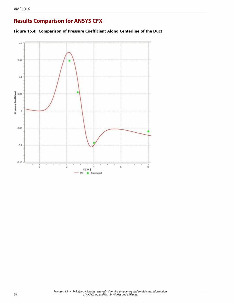
Figure 16.3: Comparison of Pressure Coefficient Along Centerline of the Duct
57Release 14.5 - © SAS IP, Inc. All rights reserved. - Contains proprietary and confidential information
of ANSYS, Inc. and its subsidiaries and affiliates.
VMFL016
Results Comparison for ANSYS CFX
Figure 16.4: Comparison of Pressure Coefficient Along Centerline of the Duct
Release 14.5 - © SAS IP, Inc. All rights reserved. - Contains proprietary and confidential informationof ANSYS, Inc. and its subsidiaries and affiliates.58
VMFL016

VMFL017: Transonic Flow over an RAE 2822 Airfoil
Overview
P.H. Cook, M.A. McDonald, and M.C.P. Firmin. “AEROFOIL RAE 2822 Pressure Distribu-
tion and Boundary Layer and Wake Measurements”. AGARD Advisory Report. No. 138.
1979.
Reference
ANSYS FLUENT, ANSYS CFXSolver
Compressible, turbulent flowPhysics/Models
Input File r2822.cas for ANSYS FLUENT
VMFL017B_VV017.def for ANSYS CFX
Test Case
Flow over an RAE 2822 airfoil at a free-stream Mach number of 0.73. The angle of attack is 2.79°. The
flow field is 2D, compressible (transonic), and turbulent. The geometry of the RAE 2822 airfoil is shown
in Figure 17.1: Geometry of the RAE 2822 Airfoil (p. 59). It is a thick airfoil with a chord length, c, of
1.00 m and a maximum thickness, d, of 0.121 m. The domain extends 55c from the airfoil, so that the
presence of the airfoil is not felt at the outer boundary.
Figure 17.1: Geometry of the RAE 2822 Airfoil
0.121 m
x
1.00 m
Mach Number = 0.73
Re = 6.5 x 10^6
Angle of Attack = 2.79 degrees
Static Pressure = 43765
Inlet Temperature = 300 K
Turbulent Intensity =0.05%
Turbulent Viscosity Ratio = 10
Boundary ConditionsGeometryMaterial Properties
The inlet conditions are:Chord length = 1 mFluid: Air
Mach number = 0.73Maximum thickness =
0.121 m
• Density: Ideal Gas
Re = 6.5 x 10⁶
• Viscosity: 1.983x10⁻⁵
kg/m-s
Static pressure = 43765
Pa
• Thermal conductivity: 0.0242 W/m-K
• Molecular Weight: 28.966
Inlet temperature = 300
K• Specific Heat: 1006.43 J/kg-K
59Release 14.5 - © SAS IP, Inc. All rights reserved. - Contains proprietary and confidential information
of ANSYS, Inc. and its subsidiaries and affiliates.

Boundary ConditionsGeometryMaterial Properties
Turbulent intensity =
0.05 %
Turbulent viscosity ratio
= 10
Analysis Assumptions and Modeling Notes
The implicit formulation of the density-based solver is used. The SST k-ω turbulence model is used to
account for turbulence effects. The problem is solved in steady state mode.
Results Comparison for ANSYS FLUENT
Table 17.1: Comparison of Coefficients
Ra-
tio
ANSYS FLU-
ENT
Tar-
get
Coeffi-
cients
0.9820.01650.0168Drag
0.9750.7830.803Lift
Results Comparison for ANSYS CFX
Table 17.2: Comparison of Coefficients
Ra-
tio
ANSYS
CFX
Tar-
get
Coeffi-
cients
0.9820.01650.0168Drag
0.9740.78250.803Lift
Release 14.5 - © SAS IP, Inc. All rights reserved. - Contains proprietary and confidential informationof ANSYS, Inc. and its subsidiaries and affiliates.60
VMFL017
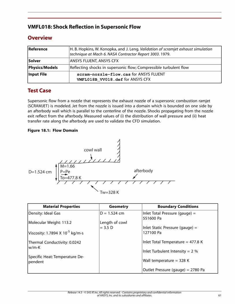
VMFL018: Shock Reflection in Supersonic Flow
Overview
H. B. Hopkins, W. Konopka, and J. Leng. Validation of scramjet exhaust simulation
technique at Mach 6. NASA Contractor Report 3003. 1979.
Reference
ANSYS FLUENT, ANSYS CFXSolver
Reflecting shocks in supersonic flow; Compressible turbulent flowPhysics/Models
Input File scram-nozzle-flow.cas for ANSYS FLUENT
VMFL018B_VV018.def for ANSYS CFX
Test Case
Supersonic flow from a nozzle that represents the exhaust nozzle of a supersonic combustion ramjet
(SCRAMJET) is modeled. Jet from the nozzle is issued into a domain which is bounded on one side by
an afterbody wall which is parallel to the centerline of the nozzle. Shocks propagating from the nozzle
exit reflect from the afterbody. Measured values of (i) the distribution of wall pressure and (ii) heat
transfer rate along the afterbody are used to validate the CFD simulation.
Figure 18.1: Flow Domain
cowl wall
afterbody
Tw=328 K
To=477.8 K
D=1.524 cm
M=1.66
P=Pe
Boundary ConditionsGeometryMaterial Properties
Inlet Total Pressure (gauge) =
551600 Pa
D = 1.524 cm
Length of cowl
= 3.5 D
Density: Ideal Gas
Molecular Weight: 113.2
Viscosity: 1.7894 X 10⁻⁵
kg/m-s
Inlet Static Pressure (gauge) =
127100 Pa
Inlet Total Temperature = 477.8 KThermal Conductivity: 0.0242
w/m-KInlet Turbulent Intensity = 2 %
Specific Heat: Temperature De-
pendent Wall temperature = 328 K
Outlet Pressure (gauge) = 2780 Pa
61Release 14.5 - © SAS IP, Inc. All rights reserved. - Contains proprietary and confidential information
of ANSYS, Inc. and its subsidiaries and affiliates.
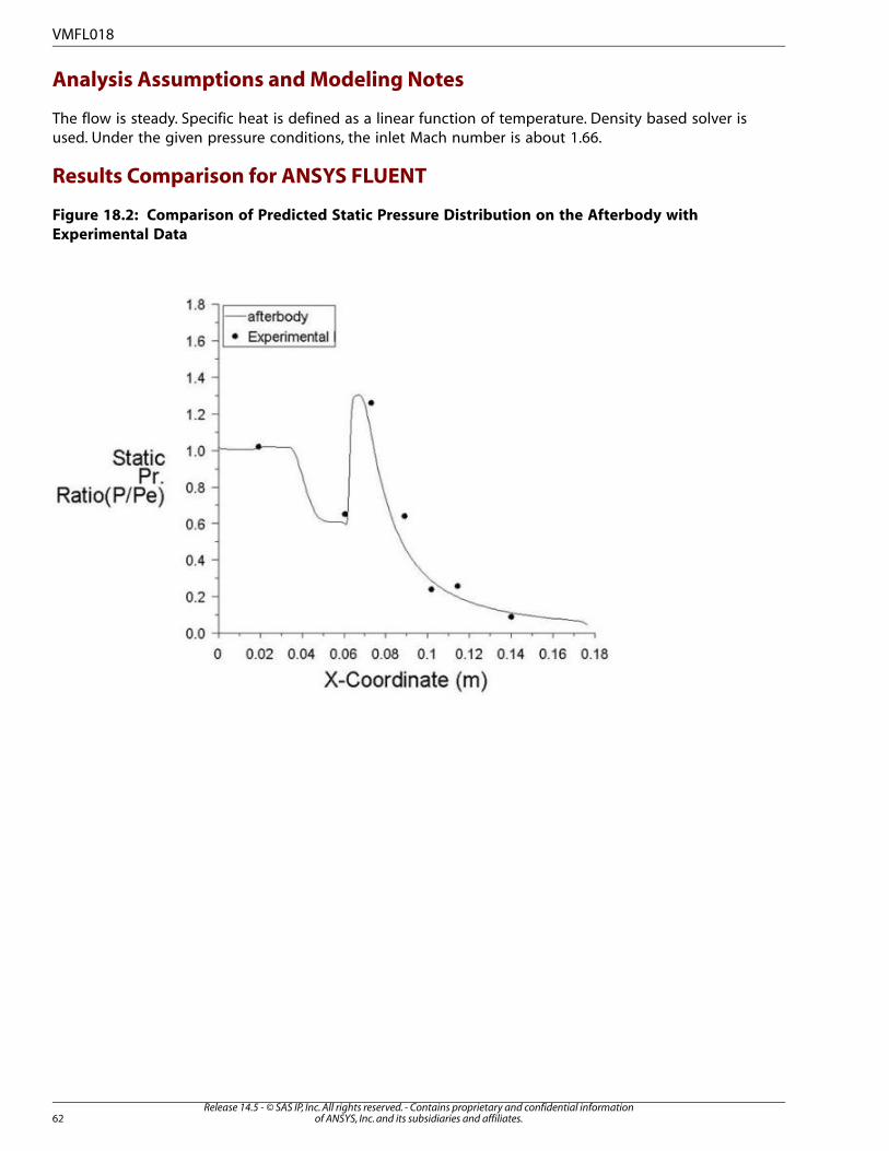
Analysis Assumptions and Modeling Notes
The flow is steady. Specific heat is defined as a linear function of temperature. Density based solver is
used. Under the given pressure conditions, the inlet Mach number is about 1.66.
Results Comparison for ANSYS FLUENT
Figure 18.2: Comparison of Predicted Static Pressure Distribution on the Afterbody with
Experimental Data
Release 14.5 - © SAS IP, Inc. All rights reserved. - Contains proprietary and confidential informationof ANSYS, Inc. and its subsidiaries and affiliates.62
VMFL018

Figure 18.3: Comparison of Predicted Total Heat Flux Along the Afterbody with Experimental
Data
Results Comparison for ANSYS CFX
Figure 18.4: Comparison of Predicted Static Pressure Distribution on the Afterbody with
Experimental Data
63Release 14.5 - © SAS IP, Inc. All rights reserved. - Contains proprietary and confidential information
of ANSYS, Inc. and its subsidiaries and affiliates.
VMFL018

Figure 18.5: Comparison of Predicted Total Heat Flux Along the Afterbody with Experimental
Data
Release 14.5 - © SAS IP, Inc. All rights reserved. - Contains proprietary and confidential informationof ANSYS, Inc. and its subsidiaries and affiliates.64
VMFL018

VMFL019: Transient Flow near a Wall Set in Motion
Overview
Boundary Layer Theory, H. Schlichting & K. Gersten, 8th Edition, 1999; Page
126-127.
Reference
ANSYS FLUENT, ANSYS CFXSolver
Unsteady flow, moving wallPhysics/Models
Input File VMFL019_FLUENT.cas for ANSYS FLUENT
VMFL019_CFX.def for ANSYS CFX
Test Case
Flow near a wall suddenly set into motion is modeled. The start up flow is modeled as a transient
problem with a constant wall-velocity at t (time) > 0. The flow is highly viscous and the velocity is 0 at
t= 0.
Figure 19.1: Flow Domain
Moving Wall
Inlet
Fixed Wall
Outlet
Boundary ConditionsGeometryMaterial Properties
Velocity of the moving wall =
0.02 m/s
Dimensions of the do-
main: 0.75 m X 0.3 mDensity = 1000 kg/m
3
Viscosity = 1 kg/m-sGauge Pressure at Inlet = 0
N/m2
Gauge Pressure at Outlet = 0
N/m2
Analysis Assumptions and Modeling Notes
The pressure based solver is used in ANSYS FLUENT. Pressure boundaries are specified to model the
driving head in the direction of flow. The fluid is at rest initially (t = 0). The similarity parameter is defined
as:
η ν( ) = ( )
65Release 14.5 - © SAS IP, Inc. All rights reserved. - Contains proprietary and confidential information
of ANSYS, Inc. and its subsidiaries and affiliates.

Where ν is the kinematic viscosity.
Results Comparison using ANSYS FLUENT
Figure 19.2: Comparison of Velocity Profile Near the Wall at Outlet
Results Comparison using ANSYS CFX
Figure 19.3: Comparison of Velocity Profile Near the Wall at Outlet
Release 14.5 - © SAS IP, Inc. All rights reserved. - Contains proprietary and confidential informationof ANSYS, Inc. and its subsidiaries and affiliates.66
VMFL019

VMFL020: Adiabatic Compression of Air in Cylinder by a Reciprocating Piston
Overview
L. D. Russell and G. A. Adebiyi. “Classical Thermodynamics”. Saunders College Pub-
lishing. Philadelphia, PA (Now Oxford University Press). 1993.
Reference
ANSYS FLUENT (ANSYS CFX simulation is not available for this case)Solver
Dynamic Mesh, Transient flow with ideal gas effectsPhysics/Models
box2d_remesh.casInput File
Test Case
Air undergoes adiabatic compression due to the movement of a piston inside a rectangular box, repres-
enting a cylinder geometry in 2–D as shown in Figure 20.1: In-Cylinder Piston Description (p. 67). The
Top Dead Center (TDC) corresponds to a crank angle of 360°. The piston moves back after reaching
TDC.
Figure 20.1: In-Cylinder Piston Description
crank angle
ϑ
67Release 14.5 - © SAS IP, Inc. All rights reserved. - Contains proprietary and confidential information
of ANSYS, Inc. and its subsidiaries and affiliates.

Figure 20.2: Flow Domain
TDC
BDC
8 m
8 m
10
m
PISTON
Boundary ConditionsGeometryMaterial Properties
Movement of the piston modeled us-
ing deforming mesh
Length of the block
= 10 m
Ideal gas law for density
Viscosity = 1.7894 X 10⁻⁵
kg/m-s Width of the block =
8 m
Analysis Assumptions and Modeling Notes
The compression within the cylinder is assumed to be adiabatic. The Spring-based smoothing method
with local remeshing is used for modeling the dynamic mesh motion.
Release 14.5 - © SAS IP, Inc. All rights reserved. - Contains proprietary and confidential informationof ANSYS, Inc. and its subsidiaries and affiliates.68
VMFL020

Results Comparison
Figure 20.3: Comparison of Static Temperature Variation with Time
Figure 20.4: Comparison of Static Pressure Variation with Time
69Release 14.5 - © SAS IP, Inc. All rights reserved. - Contains proprietary and confidential information
of ANSYS, Inc. and its subsidiaries and affiliates.
VMFL020

Release 14.5 - © SAS IP, Inc. All rights reserved. - Contains proprietary and confidential informationof ANSYS, Inc. and its subsidiaries and affiliates.70

VMFL021: Cavitation over a Sharp-Edged Orifice Case A: High Inlet Pressure
Overview
W.H. Nurick. “Orifice Cavitation and Its Effects on Spray Mixing”. Journal of Fluids
Eng.. Vol.98. 681-687. 1976.
Reference
ANSYS FLUENT, ANSYS CFXSolver
Turbulent multiphase flow with cavitation and phase changePhysics/Models
Input File cav_orifice_HP.cas for ANSYS FLUENT
VMFL021B_VV021.def for ANSYS CFX
Test Case
A steady, axisymmetric, multiphase (water/steam) flow, with phase change taking place. Due to sudden
contraction a low pressure region occurs near the sharp edge which results in cavitation. Figure 21.1: Flow
Domain (p. 71)depicts the orifice geometry. Flow direction is from left to right.
Figure 21.1: Flow Domain
L1 L2
P1 P2
r 1
r 2
vapor
liquid jet
vapor
Boundary Condi-
tions
GeometryMaterial Properties
P1 =
250,000,000 Pa
L1 =
1.60
cm
Liquid: Water
Density : 1000
kg/m3 P2 = 95,000 Pa
L2 =
3.20
cm
Viscosity: 0.001
kg/m-s
Gas: Water-Vapor
T = 300 K
Pvapor = 3,540
Par1 =
1.15
cmDensity: 0.02558
kg/m3
71Release 14.5 - © SAS IP, Inc. All rights reserved. - Contains proprietary and confidential information
of ANSYS, Inc. and its subsidiaries and affiliates.

Boundary Condi-
tions
GeometryMaterial Properties
r2 =
0.40
cm
Viscosity: 1.26x10⁻⁶
kg/m-s
Analysis Assumptions and Modeling Notes
The flow is steady and incompressible. Pressure based solver is used. Standard k-ε model with standard
wall functions is used for turbulence. The Zwart-Gerber-Belamri cavitation model is applied together
with mixture multiphase model.
For analysis of results, we calculate and compare the discharge coefficient with the experimental data.
The coefficient of discharge,, is the ratio of the mass flow rate through the nozzle to the theoretical
maximum mass flow rate:
=−
In the above equation, is the mass flow rate as calculated by the CFD solver.
Results Comparison for ANSYS FLUENT
Table 21.1: Comparison of Discharge Coefficient
Ra-
tio
ANSYS FLU-
ENT
Tar-
get
1.0180.6310.620Coefficient of Dis-
charge
Release 14.5 - © SAS IP, Inc. All rights reserved. - Contains proprietary and confidential informationof ANSYS, Inc. and its subsidiaries and affiliates.72
VMFL021
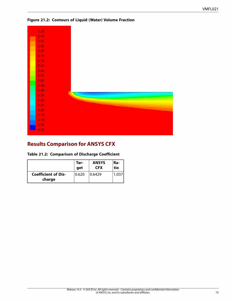
Figure 21.2: Contours of Liquid (Water) Volume Fraction
Results Comparison for ANSYS CFX
Table 21.2: Comparison of Discharge Coefficient
Ra-
tio
ANSYS
CFX
Tar-
get
1.0370.64290.620Coefficient of Dis-
charge
73Release 14.5 - © SAS IP, Inc. All rights reserved. - Contains proprietary and confidential information
of ANSYS, Inc. and its subsidiaries and affiliates.
VMFL021

Release 14.5 - © SAS IP, Inc. All rights reserved. - Contains proprietary and confidential informationof ANSYS, Inc. and its subsidiaries and affiliates.74

VMFL022: Cavitation over a Sharp-Edged Orifice Case B: Low Inlet Pressure
Overview
W.H. Nurick. “Orifice Cavitation and Its Effects on Spray Mixing”. Journal of Fluids
Eng.. Vol.98. 681-687. 1976.
Reference
ANSYS FLUENT, ANSYS CFXSolver
Turbulent multiphase flow with cavitation and phase changePhysics/Models
Input File cav_orifice_LP.cas for ANSYS FLUENT
VMFL022B_VV022.def for ANSYS CFX
Test Case
A steady, axisymmetric, multiphase (water/steam) flow, with phase change taking place. Due to sudden
contraction a low pressure region occurs near the sharp edge which results in a weak cavitation. Fig-
ure 22.1: Flow Domain (p. 75) depicts the orifice geometry. Flow direction is from left to right.
Figure 22.1: Flow Domain
L1 L2
P1 P2
r 1
r 2
vapor
liquid jet
vapor
Boundary Condi-
tions
GeometryMaterial Properties
P1 = 250,000 PaL1 =
1.60
cm
Liquid: Water
Density: 1000
kg/m3
P2 = 95,000 Pa
T = 300 KL2 =
3.20
cm
Viscosity: 0.001
kg/m-s
Gas: Water-Vapor
Pvapor = 3,540
Pa
r1 =
1.15
cmDensity: 0.02558
kg/m3
75Release 14.5 - © SAS IP, Inc. All rights reserved. - Contains proprietary and confidential information
of ANSYS, Inc. and its subsidiaries and affiliates.

Boundary Condi-
tions
GeometryMaterial Properties
r2 =
0.40
cm
Viscosity: 1.26x10⁻⁶
kg/m-s
Analysis Assumptions and Modeling Notes
The flow is steady and incompressible. Pressure based solver is used. Standard k-ε model with standard
wall functions is used for turbulence. The Zwart-Gerber-Belamri cavitation model is applied together
with mixture multiphase model.
For analysis of results, we calculate and compare the discharge coefficient with the experimental data.
The coefficient of discharge,, is the ratio of the mass flow rate through the nozzle to the theoretical
maximum mass flow rate:
=−
In the above equation, is the mass flow rate as calculated by the CFD solver.
Results Comparison for ANSYS FLUENT
Table 22.1: Comparison of Discharge Coefficient
RatioANSYS FLUENTTarget
0.9960.7770.780Coefficient of Discharge
Release 14.5 - © SAS IP, Inc. All rights reserved. - Contains proprietary and confidential informationof ANSYS, Inc. and its subsidiaries and affiliates.76
VMFL022

Figure 22.2: Contours of Liquid (Water) Volume Fraction
Results Comparison for ANSYS CFX
Table 22.2: Comparison of Discharge Coefficient
RatioANSYS CFXTarget
1.0320.80510.780Coefficient of Discharge
77Release 14.5 - © SAS IP, Inc. All rights reserved. - Contains proprietary and confidential information
of ANSYS, Inc. and its subsidiaries and affiliates.
VMFL022

Release 14.5 - © SAS IP, Inc. All rights reserved. - Contains proprietary and confidential informationof ANSYS, Inc. and its subsidiaries and affiliates.78

VMFL023: Oscillating Laminar Flow Around a Circular Cylinder
Overview
Reference F. M. White. “Fluid Mechanics”. 3rd Edition. McGraw-Hill Book Co.. New
York, NY. 1994.
S.J. Kim and C.M. Lee. “Numerical Investigation of Cross-Flow Around a Cir-
cular Cylinder at a Low-Reynolds Number Flow Under an Electromagnetic
Force”. KSME International Journal. Vol 16. No. 3. 363-375. 2002.
ANSYS FLUENT, ANSYS CFXSolver
Laminar, transient flowPhysics/Models
Input File cyl_2d.cas for ANSYS FLUENT
VMFL023B_osc_cyl.def for ANSYS CFX
Test Case
The purpose of this case is to validate the ability of ANSYS FLUENT and ANSYS CFX to predict the flow
structure as well as the reattachment length and Strouhal number against experimental results. The
present calculations are confined to the low-Reynolds-number regime (Re = 100), which encompasses
unsteady asymmetric flow.
Figure 23.1: Flow Domain
20D
D
Flow
U = 1 m/s
10D
y
x
∞
Table 23.1: Materials, Geometry, and Boundary Conditions
Boundary Condi-
tions
GeometryMaterial Proper-
ties
U ∞ = 1 m/sDiameter of the cylinder
= 2 m
Density: 1
kg/m3
Viscosity: 0.02
kg/m-s
79Release 14.5 - © SAS IP, Inc. All rights reserved. - Contains proprietary and confidential information
of ANSYS, Inc. and its subsidiaries and affiliates.

Analysis Assumptions and Modeling Notes
The flow is laminar, and unsteady. An FFT analysis of the lift coefficient on the cylinder wall is presented
to determine the frequency of oscillations. The Strouhal number corresponding to the maximum mag-
nitude of oscillations is presented in the Table below.
Results Comparison for ANSYS FLUENT
The formula for the Strouhal number is S = (N * D)/U∞, where N is the frequency, D is the diameter of
the cylinder, and U∞ is the freestream velocity.
Table 23.2: Predicted Strouhal Number for Re = 100
RatioANSYS FLUENTTarget
1.0480.1730.165Strouhal Number
Results Comparison for ANSYS CFX
Table 23.3: Predicted Strouhal Number for Re = 100
RatioANSYS CFXTarget
1.0400.1720.165Strouhal Number
Release 14.5 - © SAS IP, Inc. All rights reserved. - Contains proprietary and confidential informationof ANSYS, Inc. and its subsidiaries and affiliates.80
VMFL023

VMFL024: Interface of Two Immiscible Liquids in a Rotating Cylinder
Overview
T. Sugimoto and M. Iguchi. “Behavior of Immiscible Two Liquid Layers Contained in
Cylindrical Vessel Suddenly Set in Rotation”. ISIJ Int., 42. 338-343. 2002.
Reference
ANSYS FLUENT, ANSYS CFXSolver
Multiphase (Volume of Fluid), transient flow, body forcePhysics/Models
Input File rot-cyl_2liq_vof.cas for ANSYS FLUENT
VMFL024B_rot_cyl.def for ANSYS CFX
Test Case
Laminar interface between two immiscible liquids, water and silicon oil, inside a vertical cylinder which
is set in rotation starting from a state of rest. The silicone oil layer rests on top of the water due to its
lower density. The cylinder is sealed at the top. The vessel is set to rotate with a constant angular velocity.
Figure 24.1: Flow Domain
46 mmφ
Silicone Oil
Water
ω
120 mm
Hso
Hwg
Table 24.1: Materials, Geometry, and Boundary Conditions
Boundary ConditionsGeometryMaterial Properties
All walls are set up at rotational speed
of 2.39577 rad/s
Diameter of the cylinder =
46mm
Water :
81Release 14.5 - © SAS IP, Inc. All rights reserved. - Contains proprietary and confidential information
of ANSYS, Inc. and its subsidiaries and affiliates.

Boundary ConditionsGeometryMaterial Properties
Density: 1030
kg/m3
Height of the cylinder =
120 mm
Viscosity: 0.00103
kg/m-s
Silicon Oil:
Density: 935
kg/m3
Viscosity: 0.0103
kg/m-s
Analysis Assumptions and Modeling Notes
The flow is laminar, unsteady and axisymmetric. Non-dimensionalized swirl velocity, defined as Swirl
velocity / (Rotational speed X Cylinder radius) is used to validate the results.
Results Comparison for ANSYS FLUENT
Table 24.2: Comparison of the Non-Dimensional Swirl Velocity at Various Radial Locations (for a
Given Axial Location, X = 20mm) at Time t = 80 s
Ra-
tio
ANSYS FLU-
ENT
Tar-
get
Radial locations (at x = 20
mm)
0.9970.20930.214.83 mm
1.0020.41090.419.43 mm
1.0030.62210.6214.26 mm
Results Comparison for ANSYS CFX
Table 24.3: Comparison of the Non-Dimensional Swirl Velocity at Various Radial Locations (for a
Given Axial Location, X = 20mm) at Time t = 80 s
Ra-
tio
ANSYS
CFX
Tar-
get
Radial locations (at x = 20
mm)
0.9970.20930.214.83 mm
1.0020.41090.419.43 mm
1.0030.62210.6214.26 mm
Release 14.5 - © SAS IP, Inc. All rights reserved. - Contains proprietary and confidential informationof ANSYS, Inc. and its subsidiaries and affiliates.82
VMFL024

VMFL025: Turbulent Non-Premixed Methane Combustion with Swirling Air
Overview
Reference P.A.M. Kalt, Y.M. Al-Abdeli, A.R. Masri, and R.S. Barlow . “Swirling turbulent
non-premixed flames of methane: Flow field and compositional structure”.
Proc. Combust. Inst., 29. 1913-1919. 2002.
Y.M. Al-Abdeli and A.R. Masri. “Stability Characteristics and Flow Fields of
Turbulent Swirling Jet Flows”. Combust. Theory and Modeling, 7. 731-766.
2003.
ANSYS FLUENT, ANSYS CFXSolver
Turbulent swirling flow with reaction, non-premixed combustion model, Radiation
heat transfer, Discrete ordinates method
Physics/Models
Input File non-premix_17k-final.cas for ANSYS FLUENT
VMFL025B_CFX for ANSYS CFX
Test Case
Air and Methane enter as separate streams into an annular chamber. Air issues as a swirling jet and
also as a separate co-flowing stream with axial velocity. Both the air streams are free of methane. Species
mixing and combustion take place in the axisymmetric chamber. Radiative heat transfer is taken into
account.
Figure 25.1: Flow Domain
co-owing air inlet
swirling air inlet
methane inlet
axis
outlet
Boundary ConditionsGeometryMaterial Properties
Methane inlet velocity: 32.7
m/s
The fuel (methane only) inlet has
a diameter of 3.6 mm.
Species mixture proper-
ties specified through
PDF fileAxial velocity of swirling air:
38.2 m/s
The air inlet for the annular
shroud has an inner diameter ofViscosity: 1.72 x 10-05
kg/m-sSwirl velocity of air: 19.1 m/s
50mm and an outer diameter of
60 mm.
Refractive Index = 1Co-flowing air velocity: 20
m/sCo-flowi ng air inlet has an outer
diameter of 310 mm.
83Release 14.5 - © SAS IP, Inc. All rights reserved. - Contains proprietary and confidential information
of ANSYS, Inc. and its subsidiaries and affiliates.

Boundary ConditionsGeometryMaterial Properties
Walls are adiabatic
Analysis Assumptions and Modeling Notes
The flow is steady. Realizable k-ε is used to model turbulence. Discrete ordinates method used to
model radiation. The walls are treated as adiabatic. Non-premixed combustion model is used to model
reactions.
Results Comparison ANSYS FLUENT
Figure 25.2: Comparison of Axial Velocity at X = 40mm
Release 14.5 - © SAS IP, Inc. All rights reserved. - Contains proprietary and confidential informationof ANSYS, Inc. and its subsidiaries and affiliates.84
VMFL025

Figure 25.3: Comparison of Swirl Velocity at X = 40mm
85Release 14.5 - © SAS IP, Inc. All rights reserved. - Contains proprietary and confidential information
of ANSYS, Inc. and its subsidiaries and affiliates.
VMFL025

Figure 25.4: Comparison of Temperature at X = 40mm
Release 14.5 - © SAS IP, Inc. All rights reserved. - Contains proprietary and confidential informationof ANSYS, Inc. and its subsidiaries and affiliates.86
VMFL025

Figure 25.5: Comparison of Mass Fraction of CO at X = 40mm
87Release 14.5 - © SAS IP, Inc. All rights reserved. - Contains proprietary and confidential information
of ANSYS, Inc. and its subsidiaries and affiliates.
VMFL025

Results Comparison for ANSYS CFX
Figure 25.6: Comparison of Axial Velocity at X = 40mm
Figure 25.7: Comparison of Swirl Velocity at X = 40mm
Release 14.5 - © SAS IP, Inc. All rights reserved. - Contains proprietary and confidential informationof ANSYS, Inc. and its subsidiaries and affiliates.88
VMFL025
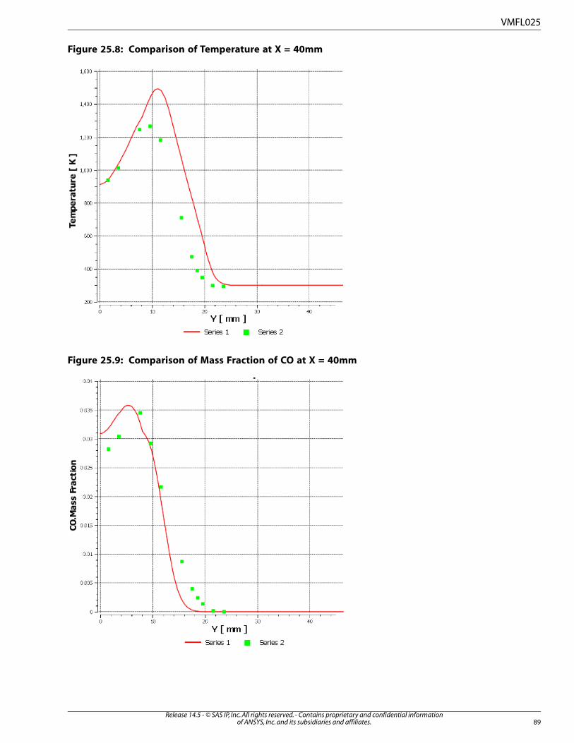
Figure 25.8: Comparison of Temperature at X = 40mm
Figure 25.9: Comparison of Mass Fraction of CO at X = 40mm
89Release 14.5 - © SAS IP, Inc. All rights reserved. - Contains proprietary and confidential information
of ANSYS, Inc. and its subsidiaries and affiliates.
VMFL025

Release 14.5 - © SAS IP, Inc. All rights reserved. - Contains proprietary and confidential informationof ANSYS, Inc. and its subsidiaries and affiliates.90

VMFL026: Supersonic Flow with Real Gas Effects inside a Shock Tube
Overview
K. Mohamed and M. Paraschivoiu. “Real Gas Numerical Simulation of Hydrogen Flow”.
2nd International Energy Conversion Engineering Conference. Providence, Rhode Is-
land. Aug. 16-19, 2004.
Reference
ANSYS FLUENT, ANSYS CFXSolver
Transient Compressible flow, Real Gas effects, ShockPhysics/Models
Input File realgas_shock-tube.cas for ANSYS FLUENT
VMFL026B_CFX.def for ANSYS CFX
Test Case
Transient flow inside a hydrogen filled shock tube is modeled. A diaphragm separating regions of high
and low pressures ruptures at t = 0 thereby creating a shock wave in the tube.
Figure 26.1: Flow Domain
L
L = 1.0 mArea = 0.01 m
2
Table 26.1: Materials, Geometry, and Boundary Conditions
Boundary ConditionsGeometryMaterial Properties
Cell zone conditions are specified
with high pressure and low pres-
sure properties of hydrogen
Length of the tube = 1
m
Area of cross section =
0.01 m2
Density is specified using
the Aungier-Redlich-Kwong
real gas model
Analysis Assumptions and Modeling Notes
The flow is compressible and unsteady by nature. Real gas effects are significant in the pressure range
considered here.
91Release 14.5 - © SAS IP, Inc. All rights reserved. - Contains proprietary and confidential information
of ANSYS, Inc. and its subsidiaries and affiliates.

Results Comparison for ANSYS FLUENT
Figure 26.2: Comparison of Static Temperature Along Centerline of the Tube
Figure 26.3: Comparison of Static Pressure Along Centerline of the Tube
Release 14.5 - © SAS IP, Inc. All rights reserved. - Contains proprietary and confidential informationof ANSYS, Inc. and its subsidiaries and affiliates.92
VMFL026

Results Comparison for ANSYS CFX
Figure 26.4: Comparison of Static Temperature Along Centerline of the Tube
Figure 26.5: Comparison of Static Pressure Along Centerline of the Tube
93Release 14.5 - © SAS IP, Inc. All rights reserved. - Contains proprietary and confidential information
of ANSYS, Inc. and its subsidiaries and affiliates.
VMFL026

Release 14.5 - © SAS IP, Inc. All rights reserved. - Contains proprietary and confidential informationof ANSYS, Inc. and its subsidiaries and affiliates.94

VMFL027: Turbulent Flow over a Backward-Facing Step
Overview
D.M. Driver and H.L. Seegmiller. "Features of a Reattaching Turbulent Shear Layer in
Divergent Channel Flow". AIAA Journal. Vol. 23, No. 2. 163-171. Feb. 1985.
Reference
ANSYS FLUENT, ANSYS CFXSolver
2-D turbulent flow with separation and reattachment, realizable k-ε modelPhysics/Models
Input File drivseeg-rke-neqwf.cas for ANSYS FLUENT
VMFL027B_step.def for ANSYS CFX
Test Case
Turbulent flow over a backward facing step is modeled. The flow separates at the step and reattaches
on the wall downstream, enclosing a region of recirculation. The inlet is at 4 H upstream and the outlet
at 30 H downstream from the location of the step, where H is the step height. Reynolds number based
on the step-height is about 28,000.
Figure 27.1: Flow Domain
Step
Inlet Outlet
Table 27.1: Materials, Geometry, and Boundary Conditions
Boundary ConditionsGeometryMaterial Properties
Inlet velocity specified as fully de-
veloped turbulent velocity profile
Step height = 1m
Total length of the channel
= 34 m
Density : 1 kg/m3
Viscosity: 0.0001
kg/m-s
Height of the channel = 9 m
Analysis Assumptions and Modeling Notes
The flow is steady. Realizable k-ε model was used to model turbulence.
95Release 14.5 - © SAS IP, Inc. All rights reserved. - Contains proprietary and confidential information
of ANSYS, Inc. and its subsidiaries and affiliates.

Results Comparison for ANSYS FLUENT
Figure 27.2: Comparison of Skin Friction Coefficient Along the Wall
Release 14.5 - © SAS IP, Inc. All rights reserved. - Contains proprietary and confidential informationof ANSYS, Inc. and its subsidiaries and affiliates.96
VMFL027

Results Comparison for ANSYS CFX
Figure 27.3: Comparison of Skin Friction Coefficient Along the Wall
97Release 14.5 - © SAS IP, Inc. All rights reserved. - Contains proprietary and confidential information
of ANSYS, Inc. and its subsidiaries and affiliates.
VMFL027

Release 14.5 - © SAS IP, Inc. All rights reserved. - Contains proprietary and confidential informationof ANSYS, Inc. and its subsidiaries and affiliates.98

VMFL028: Turbulent Heat Transfer in a Pipe Expansion
Overview
Baughn et al.. “Local Heat Transfer Downstream of an Abrupt Expansion in a Circular
Channel With Constant Wall Heat Flux”. Journal of Heat Transfer, 106. 789-796. 1984.
Reference
ANSYS FLUENT, ANSYS CFXSolver
Heat transfer, turbulent flow with recirculation and reattachmentPhysics/Models
Input File bghnexp.cas for ANSYS FLUENT
VMFL028B_pipe_expansion.def for ANSYS CFX
Test Case
Fully developed turbulent flow through an axisymmetric pipe expansion is modeled. The flow reattaches
to the pipe wall downstream of the expansion, enclosing a zone of recirculation. The pipe wall down-
stream of the expansion is heated at a constant rate. Inlet to the computational domain is placed at 1
step height upstream of the expansion and the outlet at 40 step-heights downstream.
Figure 28.1: Flow Domain
H = 1 m
q” = 0 W/m2
r
R
40 H
q” = 0.3 W/m 2
velocity
inlet
x
H
axis
pressure
outlet
Boundary ConditionsGeometryMaterial Properties
Inlet velocity: Specified by fully
developed turbulent velocity pro-
file
Pipe radius before ex-
pansion = 0.667 m
Pipe radius after expan-
sion = 1.6667 m
Density: 1.225 kg/m3
Viscosity: 1.68318e-5kg/m-s
Specific Heat: 1006.43 J/kg-K Inlet temperature = 273 K
Heat flux across the wall after ex-
pansion = 0.3 W/m2
Thermal Conductivity: 0.0242
W/m-K
Analysis Assumptions and Modeling Notes
Steady flow in axisymmetric domain. The wall upstream of expansion is adiabatic.
99Release 14.5 - © SAS IP, Inc. All rights reserved. - Contains proprietary and confidential information
of ANSYS, Inc. and its subsidiaries and affiliates.

Results Comparison for ANSYS FLUENT
Figure 28.2: Nusselts Number Variation along the Heat Wall
Results Comparison for ANSYS CFX
Figure 28.3: Nusselts Number Variation along the Heat Wall
Release 14.5 - © SAS IP, Inc. All rights reserved. - Contains proprietary and confidential informationof ANSYS, Inc. and its subsidiaries and affiliates.100
VMFL028

VMFL029: Anisotropic Conduction Heat Transfer
Overview
Reference
ANSYS FLUENT (ANSYS CFX simulation is not available for this case)Solver
Heat conduction, anisotropic conductivityPhysics/Models
aniso.casInput File
Test Case
Heat conduction in a solid with anisotropic thermal conductivity is modeled. A square domain is con-
sidered. Two opposite walls are maintained at uniform temperatures. Conductivity of the solid material
is specified using matrix components to account for the anisotropy. The simulation results are compared
with analytical solution for temperature distribution.
Figure 29.1: Domain
Boundary ConditionsGeometryMaterial Properties
Fixed wall temperatures = 100 K and
200K respectively
Dimensions of the
domain: 1m X 1 m
Density of solid = 2719
kg/m3
User-defined profile for temperature
distribution on the other two wallsSpecific heat = 871 J/kg-K
Thermal conductivity: Aniso-
tropic
Analysis Assumptions and Modeling Notes
Steady state conduction. Anisotropic conductivity modeled by specified matrix components for the
solid conductivity.
101Release 14.5 - © SAS IP, Inc. All rights reserved. - Contains proprietary and confidential information
of ANSYS, Inc. and its subsidiaries and affiliates.

Results Comparison
Figure 29.2: Comparison of Temperature Distribution at X = 0.5 m
Release 14.5 - © SAS IP, Inc. All rights reserved. - Contains proprietary and confidential informationof ANSYS, Inc. and its subsidiaries and affiliates.102
VMFL029

VMFL030: Turbulent Flow in a 90° Pipe-Bend
Overview
M. M. Enayet, M. M. Gibson, A. M. K. P. Taylor, and M. Yianneskis. “Laser-Doppler
Measurements of Laminar and Turbulent Flow in a Pipe Bend”. Znt. J. Heat &
Fluid Flow. Vol. 3. 213-219. 1982.
Reference
ANSYS FLUENT, ANSYS CFXSolver
3–D Turbulent flow with separation, RNG k-ε model with non-equilibrium wall
functions
Physics/Models
Input File pipebnd-rng-noneq.cas for ANSYS FLUENT
VMFL030B_vv030.def for ANSYS CFX
Test Case
Turbulent flow through a 90° circular pipe bend is modeled. The flow separates and reattaches around
the bend. Due to symmetry of the flow field only half of the domain is modeled. Velocity profile at an
angle of 75° (as measured from the inlet) is used to validate the simulation.
Figure 30.1: Flow Domain
plane at 75 deg
symmetry plane
outlet
inletZ Y
X
Boundary ConditionsGeometryMaterial Properties
Inlet velocity: Fully developed turbulent
profile for z-velocity.
Radius of the pipe
= 0.5 mDensity: 1 kg/m
3
Viscosity: 2.3256 x 10-05
kg/m-sNon components in other directions
Analysis Assumptions and Modeling Notes
The flow is steady. RNG k- ε is used to model turbulence along with non-equilibrium wall functions.
103Release 14.5 - © SAS IP, Inc. All rights reserved. - Contains proprietary and confidential information
of ANSYS, Inc. and its subsidiaries and affiliates.

Results Comparison for ANSYS FLUENT
Figure 30.2: Comparison of Velocity Magnitude (m/s) at 75° Along the Bend
Results Comparison for ANSYS CFX
Figure 30.3: Comparison of Velocity Magnitude (m/s) at 75° Along the Bend
Release 14.5 - © SAS IP, Inc. All rights reserved. - Contains proprietary and confidential informationof ANSYS, Inc. and its subsidiaries and affiliates.104
VMFL030

VMFL031: Turbulent Flow Behind an Open-Slit V Gutter
Overview
J.-T. Yang and G.-L. Tsai. “Near-wake flow of a v-gutter with slit bleed”. Journal
of Fluid Engineering. Vol. 115. 13-20. March, 1993.
Reference
ANSYS FLUENT, ANSYS CFXSolver
Turbulent flowPhysics/Models
Input File spltvee.cas for ANSYS FLUENT
VMFL031B_veesplit.def for ANSYS CFX
Test Case
The near-wake flow structure behind an open-slit V gutter at airflow speed of 20 m/s is modeled. The
interaction between the flow penetrating through the open slit and the shear layer results in an asym-
metric wake flow structure. The size of the entire recirculation zone shifts toward one of the two wings
due to the Coand effect.
Figure 31.1: Flow Domain
H
L
a
bφ
Boundary Condi-
tions
Geo-
metry
Material Properties
uinlet = 20 m/sL =
40
cm
Density: 1 kg/m3
Viscosity: 1.8333 X 10-05
kg/m-s
kinlet = 0.04335
m2/s
2
H =
10
cmεinlet = 0.2119
m2/s
3
a =
2
mm
105Release 14.5 - © SAS IP, Inc. All rights reserved. - Contains proprietary and confidential information
of ANSYS, Inc. and its subsidiaries and affiliates.

Boundary Condi-
tions
Geo-
metry
Material Properties
b =
22
mm
ø=
45°
Analysis Assumptions and Modeling Notes
Steady, turbulent, incompressible flow. The standard k-ε model is used for turbulence.
Results Comparison for ANSYS FLUENT
The x-velocity at x = 22 mm downstream of the split-V-gutter, is compared with experimental data.
Figure 31.2: X-Velocity at x = 22 mm Downstream of the V-Gutter
Release 14.5 - © SAS IP, Inc. All rights reserved. - Contains proprietary and confidential informationof ANSYS, Inc. and its subsidiaries and affiliates.106
VMFL031

Figure 31.3: The Coand Effect
Results Comparison for ANSYS CFX
Figure 31.4: X-Velocity at x = 22 mm Downstream of the V-Gutter
107Release 14.5 - © SAS IP, Inc. All rights reserved. - Contains proprietary and confidential information
of ANSYS, Inc. and its subsidiaries and affiliates.
VMFL031

Release 14.5 - © SAS IP, Inc. All rights reserved. - Contains proprietary and confidential informationof ANSYS, Inc. and its subsidiaries and affiliates.108
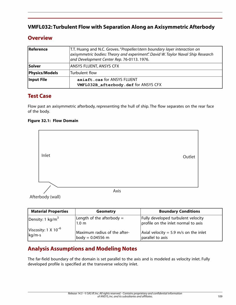
VMFL032: Turbulent Flow with Separation Along an Axisymmetric Afterbody
Overview
T.T. Huang and N.C. Groves. “Propeller/stern boundary layer interaction on
axisymmetric bodies: Theory and experiment”. David W. Taylor Naval Ship Research
and Development Center Rep. 76-0113. 1976.
Reference
ANSYS FLUENT, ANSYS CFXSolver
Turbulent flowPhysics/Models
Input File axiaft.cas for ANSYS FLUENT
VMFL032B_afterbody.def for ANSYS CFX
Test Case
Flow past an axisymmetric afterbody, representing the hull of ship. The flow separates on the rear face
of the body.
Figure 32.1: Flow Domain
Afterbody (wall)
Inlet
Axis
Outlet
Boundary ConditionsGeometryMaterial Properties
Fully developed turbulent velocity
profile on the inlet normal to axis
Length of the afterbody =
1.0 mDensity: 1 kg/m
3
Viscosity: 1 X 10⁻⁶
kg/m-sAxial velocity = 5.9 m/s on the inlet
parallel to axis
Maximum radius of the after-
body = 0.04556 m
Analysis Assumptions and Modeling Notes
The far-field boundary of the domain is set parallel to the axis and is modeled as velocity inlet. Fully
developed profile is specified at the transverse velocity inlet.
109Release 14.5 - © SAS IP, Inc. All rights reserved. - Contains proprietary and confidential information
of ANSYS, Inc. and its subsidiaries and affiliates.

Results Comparison for ANSYS FLUENT
Figure 32.2: Comparison of Pressure Coefficient Along the Afterbody Wall
Figure 32.3: Comparison of Skin Friction Coefficient Along the Afterbody Wall
Release 14.5 - © SAS IP, Inc. All rights reserved. - Contains proprietary and confidential informationof ANSYS, Inc. and its subsidiaries and affiliates.110
VMFL032

Results Comparison for ANSYS CFX
Figure 32.4: Comparison of Pressure Coefficient Along the Afterbody Wall
Figure 32.5: Comparison of Skin Friction Coefficient Along the Afterbody Wall
111Release 14.5 - © SAS IP, Inc. All rights reserved. - Contains proprietary and confidential information
of ANSYS, Inc. and its subsidiaries and affiliates.
VMFL032

Release 14.5 - © SAS IP, Inc. All rights reserved. - Contains proprietary and confidential informationof ANSYS, Inc. and its subsidiaries and affiliates.112
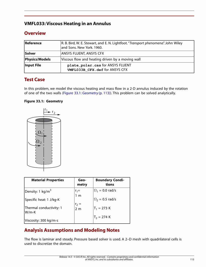
VMFL033: Viscous Heating in an Annulus
Overview
R. B. Bird, W. E. Stewart, and E. N. Lightfoot. “Transport phenomena”. John Wiley
and Sons. New York. 1960.
Reference
ANSYS FLUENT, ANSYS CFXSolver
Viscous flow and heating driven by a moving wallPhysics/Models
Input File plate_polar.cas for ANSYS FLUENT
VMFL033B_CFX.def for ANSYS CFX
Test Case
In this problem, we model the viscous heating and mass flow in a 2-D annulus induced by the rotation
of one of the two walls (Figure 33.1: Geometry (p. 113)). This problem can be solved analytically.
Figure 33.1: Geometry
rr1
2
Ω1
Ω 2
Boundary Condi-
tions
Geo-
metry
Material Properties
Ω1 = 0.0 rad/sr1=
1 mDensity: 1 kg/m
3
Specific heat: 1 J/kg-K Ω2 = 0.5 rad/s
r2 =
2 mThermal conductivity: 1
W/m-KT1 = 273 K
T2 = 274 KViscosity: 300 kg/m-s
Analysis Assumptions and Modeling Notes
The flow is laminar and steady. Pressure based solver is used. A 2–D mesh with quadrilateral cells is
used to discretize the domain.
113Release 14.5 - © SAS IP, Inc. All rights reserved. - Contains proprietary and confidential information
of ANSYS, Inc. and its subsidiaries and affiliates.

Results Comparison for ANSYS FLUENT
Normalized velocity and temperature profiles are compared with the analytical solution provided by
Bird et al (1960).
Figure 33.2: Comparison of Velocity Profile
Release 14.5 - © SAS IP, Inc. All rights reserved. - Contains proprietary and confidential informationof ANSYS, Inc. and its subsidiaries and affiliates.114
VMFL033

Figure 33.3: Comparison of Temperature Profile
Results Comparison for ANSYS CFX
Figure 33.4: Comparison of Velocity Profile
115Release 14.5 - © SAS IP, Inc. All rights reserved. - Contains proprietary and confidential information
of ANSYS, Inc. and its subsidiaries and affiliates.
VMFL033

Figure 33.5: Comparison of Temperature Profile
Release 14.5 - © SAS IP, Inc. All rights reserved. - Contains proprietary and confidential informationof ANSYS, Inc. and its subsidiaries and affiliates.116
VMFL033

VMFL034: Particle Aggregation inside a Turbulent Stirred Tank
Overview
B. Wan, T.A. Ring, K. Dhanasekharan, and J. Sanyal. “Comparison of Analytical Solu-
tions for CMSMPR Crystallizer with QMOM Population Balance Modeling in ANSYS
FLUENT”. China Particuology. Vol. 3(4). 213-218. 2005.
Reference
ANSYS FLUENT (ANSYS CFX simulation is not available for this case)Solver
Multi-phase, Population balance model, turbulent flowPhysics/Models
agglomeration.casInput File
Test Case
A 2-D approximation of a stirred tank is simulated in order to verify the population balance model that
operates in conjunction with its multiphase calculations to predict the particle size distribution within
the flow field. The flow rate at the inlet is equal to that at the outlet, allowing the mean residence time
to be calculated from the inlet flow rate (velocity x inlet area) and the “volume” (box area x unit depth)
of the box. To simulate the agitation in the tank the top and bottom walls are assumed to move in the
direction of the outlet. The flow is turbulent, steady, and incompressible. Multi-phase, with QMOM
population balance model is used for particle aggregation. The standard k-ε model is used for turbulence.
Figure 34.1: Flow Domain
Boundary ConditionsGeometryMaterial Properties
Top wall velocity: 101
m/s
Square box side = 0.1 m
Inlet/Outlet openings =
0.02 m
Density: 998.2
kg/m3
Viscosity: 0.00103
kg/m-s
Bottom wall velocity:
100 m/s
Inlet velocity = 0.005
m/s
117Release 14.5 - © SAS IP, Inc. All rights reserved. - Contains proprietary and confidential information
of ANSYS, Inc. and its subsidiaries and affiliates.
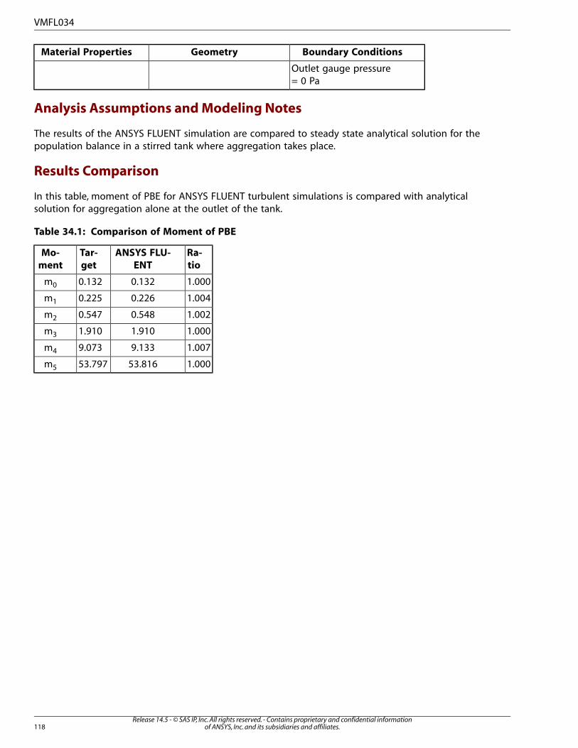
Boundary ConditionsGeometryMaterial Properties
Outlet gauge pressure
= 0 Pa
Analysis Assumptions and Modeling Notes
The results of the ANSYS FLUENT simulation are compared to steady state analytical solution for the
population balance in a stirred tank where aggregation takes place.
Results Comparison
In this table, moment of PBE for ANSYS FLUENT turbulent simulations is compared with analytical
solution for aggregation alone at the outlet of the tank.
Table 34.1: Comparison of Moment of PBE
Ra-
tio
ANSYS FLU-
ENT
Tar-
get
Mo-
ment
1.0000.1320.132m0
1.0040.2260.225m1
1.0020.5480.547m2
1.0001.9101.910m3
1.0079.1339.073m4
1.00053.81653.797m5
Release 14.5 - © SAS IP, Inc. All rights reserved. - Contains proprietary and confidential informationof ANSYS, Inc. and its subsidiaries and affiliates.118
VMFL034

VMFL035: 3-Dimensional Single-Stage Axial Compressor
Overview
Density-based solver (ANSYS FLUENT)Reference
ANSYS FLUENT, ANSYS CFXSolver
Compressible (transonic), turbulent flow, moving reference framePhysics/Models
axial-compressor.casInput File
Test Case
A 3-D model of a single-stage axial compressor is simulated. The flow through the rotor blades is
computed in a rotating reference frame, while the flow in the stator blades in a stationary frame. The
purpose of this case is to validate the performance of the pressure-based coupled solver for a compress-
ible turbomachinery problem with a mixing plane. The flow is compressible, turbulent and steady.
Figure 35.1: Flow Domain
Boundary ConditionsGeometryMaterial Properties (for
Air)
Rotational speed = 37,500
rpm
For Inlet:
Geometry is as shown in in Fig-
ure 34.1: Flow Domain (p. 117)
Number of rotor blades = 16
Density = Ideal – Gas
Molecular weight =
28.966
Number of stator blades = 40Specific heat = 1006.43
J/kg-K
• Ptotal = 1 atm
• Ttotal = 288 KViscosity - Sutherland’s
law
119Release 14.5 - © SAS IP, Inc. All rights reserved. - Contains proprietary and confidential information
of ANSYS, Inc. and its subsidiaries and affiliates.

Boundary ConditionsGeometryMaterial Properties (for
Air)
Conductivity - Kinetic
theory
Analysis Assumptions and Modeling Notes
Steady, turbulent, compressible flow. Ideal-gas law is used for density calculations and kinetic theory
for fluid viscosity and thermal conductivity. The standard k-ε model is used for turbulence. Pressure-
based coupled solver with a mixing plane at the rotor-outlet/stator-inlet interface.
Results Comparison for ANSYS FLUENT
The results of the pressure-based ANSYS FLUENT simulation are compared to the steady state solution
from the density-based solver.
Table 35.1: Comparison of Pressure and Mass Flow Rate
Ra-
tio
ANSYS FLU-
ENT
Tar-
get
1.0071.48221.4725Pressure at Stator-Outlet (atm)
1.0260.10760.1049Mass-Flow Rate at Stator-Outlet
(kg/s)
Results Comparison for ANSYS CFX
Table 35.2: Comparison of Pressure and Mass Flow Rate
Ra-
tio
ANSYS
CFX
Tar-
get
1.00201.47541.4725Pressure at Stator-Outlet (atm)
1.02760.10780.1049Mass-Flow Rate at Stator-Outlet
(kg/s)
Release 14.5 - © SAS IP, Inc. All rights reserved. - Contains proprietary and confidential informationof ANSYS, Inc. and its subsidiaries and affiliates.120
VMFL035

VMFL036: Turbulent Round Jet
Overview
D. C. Wilcox. "Turbulence Modeling for CFD". DCW Industries, Inc.. 1993.Reference
ANSYS FLUENT, ANSYS CFXSolver
Turbulent flowPhysics/Models
axjet.casTarget File
Test Case
A turbulent round jet is defined by a velocity inlet adjacent to a symmetry boundary, and exhausts into
a rectangular domain or plenum. The domain is chosen large enough and the boundary does not interfere
with the jet. The flow is turbulent and steady. The purpose of this case is to validate the performance
of the Reynolds Stress Model for turbulence.
Figure 36.1: Round Jet Geometry
y
xD
HComputational Domainu
u /2
m
m
UU 00
L
Shear
LayerCore
Boundary Condi-
tions
Geo-
metry
Material Properties
Inlet:D =
1 mDensity = 1 kg/m
3
Viscosity = 1e-05
kg/m-s
U0 = 1
m/sL =
50
mk =
0.00375
m2/s
2
H =
20
m
e =
0.00054
m2/s
3
Outlet:
121Release 14.5 - © SAS IP, Inc. All rights reserved. - Contains proprietary and confidential information
of ANSYS, Inc. and its subsidiaries and affiliates.

Boundary Condi-
tions
Geo-
metry
Material Properties
pout =
1 atm
Analysis Assumptions and Modeling Notes
Steady, turbulent, incompressible flow. The Reynolds Stress Model (RSM) is used for turbulence.
Results Comparison for ANSYS FLUENT
The jet’s spreading rate is compared to the Wilcox (1998) data for round jets. The scattering of the data
is due to the coarse triangular grid that has been used in this study. A finer grid would have produced
a much smoother computational curve.
Figure 36.2: Comparison of Results for ANSYS FLUENT
Release 14.5 - © SAS IP, Inc. All rights reserved. - Contains proprietary and confidential informationof ANSYS, Inc. and its subsidiaries and affiliates.122
VMFL036

Results Comparison for ANSYS CFX
Figure 36.3: Comparison of Results for ANSYS CFX
123Release 14.5 - © SAS IP, Inc. All rights reserved. - Contains proprietary and confidential information
of ANSYS, Inc. and its subsidiaries and affiliates.
VMFL036

Release 14.5 - © SAS IP, Inc. All rights reserved. - Contains proprietary and confidential informationof ANSYS, Inc. and its subsidiaries and affiliates.124

VMFL037: Turbulent Flow over a Forward Facing Step
Overview
S. Baker. “Regions of Recirculating Flow Associated with Two-Dimensional Steps”.
Ph.D. thesis. Department of Civil Engineering, University of Surrey. UK. 1977.
Reference
ANSYS FLUENT, ANSYS CFXSolver
SST model, turbulent flow with separation and reattachmentPhysics/Models
Input File VMFL037_ffstep.cas for ANSYS FLUENT
ffstep.def for ANSYS CFX
Test Case
Turbulent flow over a forward facing step is modeled. The flow undergoes separation and reattachment.
Figure 37.1: Flow Domain
y
x0
U
10H
5.9H
H
INLET
Free Slip Wall
No Slip Wall
14H 19H
7.3H refPref
Boundary ConditionsGeometryMaterial Properties
Inlet Velocity = 9.7 m/sStep height H =
0.0758 mDensity = 1.02 kg/m
3
Viscosity = 1.5 X 10⁻⁵
kg/m-s
Outer boundary (in transverse direction) is
modeled as slip wall
Analysis Assumptions and Modeling Notes
The flow is steady. Pressure coefficient, Cp on the wall is calculated with reference to the pressure at
point upstream of the step at coordinates as indicated in Figure 37.1: Flow Domain (p. 125).
125Release 14.5 - © SAS IP, Inc. All rights reserved. - Contains proprietary and confidential information
of ANSYS, Inc. and its subsidiaries and affiliates.

Results Comparison for ANSYS FLUENT
Figure 37.2: Comparison of Pressure Coefficient Along the Wall
Release 14.5 - © SAS IP, Inc. All rights reserved. - Contains proprietary and confidential informationof ANSYS, Inc. and its subsidiaries and affiliates.126
VMFL037

Results Comparison for ANSYS CFX
Figure 37.3: Comparison of Pressure Coefficient Along the Wall
127Release 14.5 - © SAS IP, Inc. All rights reserved. - Contains proprietary and confidential information
of ANSYS, Inc. and its subsidiaries and affiliates.
VMFL037

Release 14.5 - © SAS IP, Inc. All rights reserved. - Contains proprietary and confidential informationof ANSYS, Inc. and its subsidiaries and affiliates.128

VMFL038: Falling Film over an Inclined Plane
Overview
RB Bird. “Transport Phenomena”. WE Stewart and EN Lightfoot. Pg. 45. 2005Reference
ANSYS FLUENT, ANSYS CFXSolver
Laminar Flow, Coupled solverPhysics/Models
Input File VMFL038_FLUENT.cas for ANSYS FLUENT
VMFL038_CFX.def for ANSYS CFX
Test Case
Laminar flow of a fluid over an inclined plane, driven by the pressure difference due to gravity head is
modeled. The flow channel is inclined at an angle β = 30° with the horizontal direction.
Figure 38.1: Flow Domain
Symmetry
Wall
X
Y
Boundary ConditionsGeometryMaterial Proper-
ties
Gauge Pressure at Inlet = 0 N/m2Dimensions of the
domain:
Density = 800
kg/m3
Gauge Pressure at Outlet = -706.32
N/m2Viscosity = 1
kg/m-s
1 m X 18 m
Angle with X-axis
= 30°
Analysis Assumptions and Modeling Notes
The density based solver is used in ANSYS FLUENT. Pressure boundaries are specified to model the
driving head in the direction of flow.
129Release 14.5 - © SAS IP, Inc. All rights reserved. - Contains proprietary and confidential information
of ANSYS, Inc. and its subsidiaries and affiliates.
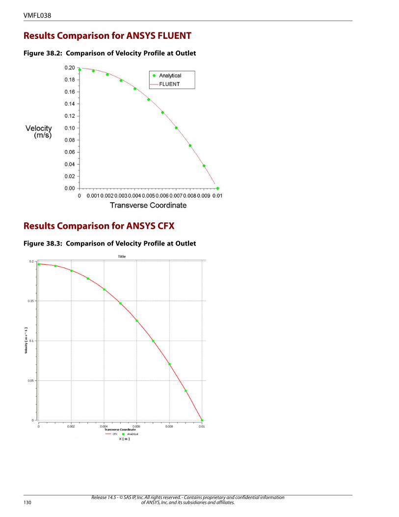
Results Comparison for ANSYS FLUENT
Figure 38.2: Comparison of Velocity Profile at Outlet
Results Comparison for ANSYS CFX
Figure 38.3: Comparison of Velocity Profile at Outlet
Release 14.5 - © SAS IP, Inc. All rights reserved. - Contains proprietary and confidential informationof ANSYS, Inc. and its subsidiaries and affiliates.130
VMFL038

VMFL039: Boiling in a Pipe with Heated Wall
Overview
G.G. Bartolomej, V.G. Brantov, Y.S. Molochnikov, Y.V. Kharitonov, V.A. Solodkii, G.N.
Batashova, V.N. Mikhailov. “An experimental investigation of the true volumetric vapour
Reference
content with subcooled boiling tubes”. Thermal Engineering. Vol. 29, No. 3. 20-22.
1982.
ANSYS CFX, ANSYS FLUENTSolver
Multiphase flow, phase change, RPI Wall boiling ModelPhysics/Models
wall-boiling.defInput File
Test Case
Bubble formation and boiling near the heated wall of a vertical pipe are modeled. Outer wall of the
pipe is heated with a constant heat flux.
Figure 39.1: Flow Domain
Z q
Mass Flow
Boundary ConditionsGeometryMaterial Properties
Mass flux at inlet = 900
kg/m2/s
Radius of the pipe
= 7.7 mm
Height of the pipe
= 2 m
Steam-Water 2-phase Flow:
• Water: continuous phase
Inlet pressure = 4.5 X 10⁶ N/m
2
131Release 14.5 - © SAS IP, Inc. All rights reserved. - Contains proprietary and confidential information
of ANSYS, Inc. and its subsidiaries and affiliates.

Boundary ConditionsGeometryMaterial Properties
Heat transfer at the wall =
570000 W/m2
• Water Steam: dispersed bubbles
Bubble diameter dependent on
fluid temperature
Analysis Assumptions and Modeling Notes
The flow is steady. SST model is used for turbulence. RPI model for wall boiling is used with a value of
0.8 for the wall area fraction affected by vapor.
Results Comparison
Figure 39.2: ANSYS FLUENT Comparison of Temperature Along the Pipe Wall
Release 14.5 - © SAS IP, Inc. All rights reserved. - Contains proprietary and confidential informationof ANSYS, Inc. and its subsidiaries and affiliates.132
VMFL039

Figure 39.3: ANSYS CFX Comparison of Temperature Along the Pipe Wall
133Release 14.5 - © SAS IP, Inc. All rights reserved. - Contains proprietary and confidential information
of ANSYS, Inc. and its subsidiaries and affiliates.
VMFL039

Release 14.5 - © SAS IP, Inc. All rights reserved. - Contains proprietary and confidential informationof ANSYS, Inc. and its subsidiaries and affiliates.134

VMFL040: Separated Turbulent Flow in Diffuser
Overview
D.M. Driver. “Reynolds shear stress measurements in a separated boundary layer flow”.
AIAA-91-1787. 1991.
Reference
ANSYS CFX, ANSYS FLUENTSolver
SST model, Adverse pressure gradient, flow separationPhysics/Models
Input Files diffuser-sep.def for ANSYS CFX
VMFL040A_diffuser-sep.cas for ANSYS FLUENT
Test Case
The test case geometry is shown in Figure 40.1: Sketch of Flow Domain (p. 135). It consists of an
axisymmetric diffuser with an internally mounted cylinder along the centre line. The curvature of the
diffuser wall results in an adverse pressure gradient. A relatively short separation region was detected
in the experiment.
Figure 40.1: Sketch of Flow Domain
Diuser
Streamline
Separation0 mm250 mm
140 mm
cylinder
y
x
This figure is not to scale.
Boundary ConditionsGeometryMaterial Properties
Velocity profile at inlet with average
velocity = 29 m/s
Diameter of the cylinder =
140 mmDensity: 1 kg/m
3
Viscosity: 1.5 X 10⁻⁵
kg/m-sOuter wall modeled as a slip (invis-
cid) wall
Length of the domain = 1100
mm
Analysis Assumptions and Modeling Notes
The flow is steady. SST model is used for turbulence.
135Release 14.5 - © SAS IP, Inc. All rights reserved. - Contains proprietary and confidential information
of ANSYS, Inc. and its subsidiaries and affiliates.

Results Comparison for ANSYS FLUENT
Figure 40.2: Comparison of Skin Friction Coefficient on the Cylinder Wall
Release 14.5 - © SAS IP, Inc. All rights reserved. - Contains proprietary and confidential informationof ANSYS, Inc. and its subsidiaries and affiliates.136
VMFL040

Results Comparison for ANSYS CFX
Figure 40.3: Comparison of Skin Friction Coefficient on the Cylinder Wall
137Release 14.5 - © SAS IP, Inc. All rights reserved. - Contains proprietary and confidential information
of ANSYS, Inc. and its subsidiaries and affiliates.
VMFL040

Release 14.5 - © SAS IP, Inc. All rights reserved. - Contains proprietary and confidential informationof ANSYS, Inc. and its subsidiaries and affiliates.138

VMFL041: Transonic Flow Over an Airfoil
Overview
P.H. Cook, M.A. McDonald, and M.C.P. Firmin. “AEROFOIL RAE 2822 - PRESSURE DIS-
TRIBUTIONS, AND BOUNDARY LAYER AND WAKE MEASUREMENTS.” AGARD Advisory
Report No. 138.
Reference
ANSYS FLUENT, ANSYS CFXSolver
Transonic flow, shock, SST modelPhysics/Models
Input File VMFL041_transonic.cas for ANSYS FLUENT
air_foil.def for ANSYS CFX
Test Case
Transoinc flow over air foil RAE 2822 is modeled for an angle of attack of 3.19°. The flow domain spans
over 100 Chord lengths in both stream-wise and transverse directions.
Figure 41.1: Flow Domain
Boundary ConditionsGeometryMaterial Properties
Velocity profile at inlet with an aver-
age velocity of 218 m/s
Chord length of the airfoil
= 1 m
Density: Ideal gas law
for Air
Viscosity: 1.831 X 10⁻⁵
kg/m-s
139Release 14.5 - © SAS IP, Inc. All rights reserved. - Contains proprietary and confidential information
of ANSYS, Inc. and its subsidiaries and affiliates.

Analysis Assumptions and Modeling Notes
The flow is steady. The inlet flow Mach number is close to transonic range. Walls are assumed to be
adiabatic.
Results Comparison for ANSYS FLUENT
Figure 41.2: Comparison of Pressure Coefficient on the Airfoil
Release 14.5 - © SAS IP, Inc. All rights reserved. - Contains proprietary and confidential informationof ANSYS, Inc. and its subsidiaries and affiliates.140
VMFL041

Results Comparison for ANSYS CFX
Figure 41.3: Comparison of Pressure Coefficient on the Airfoil
141Release 14.5 - © SAS IP, Inc. All rights reserved. - Contains proprietary and confidential information
of ANSYS, Inc. and its subsidiaries and affiliates.
VMFL041

Release 14.5 - © SAS IP, Inc. All rights reserved. - Contains proprietary and confidential informationof ANSYS, Inc. and its subsidiaries and affiliates.142

VMFL042: Turbulent Mixing of Two Streams with Different Density
Overview
Reference R.E. Uittenbogaard. “Stably Stratified Mixing Layer”. Data Report for the 14th
meeting of the IAHR Working Group on Refined Flow Modeling. 1989.
R.E. Uittenbogaard. “The Importance of Internal Waves for Mixing in a
Stratified Estaurine Tidal Flow”. 1995.
ANSYS FLUENT, ANSYS CFXSolver
SST model, mixing layer, density difference, buoyancyPhysics/Models
Input File VMFL042_mixing.cas for ANSYS FLUENT
saline-mixing_layer.def for ANSYS CFX
Test Case
Mixing of two turbulent streams of fresh water and saline water is modeled. The two streams are parallel
at the inlet and mixing proceeds downstream.
Figure 42.1: Flow Domain
y
x
Fresh water
Saline
0.323 m
40 m
0.56 m
Boundary ConditionsGeometryMaterial Properties
Fresh water inlet velocity =
0.52 m/s
Length of the mix-
ing duct = 40 mDensity of fresh water: 1015 kg/m
3
Density of saline water: 1030 kg/m3
Salt water inlet velocity = 0.32
m/sMixture kinematic diffusivity: 1 X 10
-9
m2/s
Analysis Assumptions and Modeling Notes
The flow is steady. SST model is used. Buoyancy turbulence production option is used.
143Release 14.5 - © SAS IP, Inc. All rights reserved. - Contains proprietary and confidential information
of ANSYS, Inc. and its subsidiaries and affiliates.

Results Comparison for ANSYS FLUENT
Figure 42.2: Comparison of Mass Fraction of Salt Water Across the Mixing Layer at x = 10m
Release 14.5 - © SAS IP, Inc. All rights reserved. - Contains proprietary and confidential informationof ANSYS, Inc. and its subsidiaries and affiliates.144
VMFL042

Results Comparison for ANSYS CFX
Figure 42.3: Comparison of Mass Fraction of Salt Water Across the Mixing Layer at x = 10m
145Release 14.5 - © SAS IP, Inc. All rights reserved. - Contains proprietary and confidential information
of ANSYS, Inc. and its subsidiaries and affiliates.
VMFL042

Release 14.5 - © SAS IP, Inc. All rights reserved. - Contains proprietary and confidential informationof ANSYS, Inc. and its subsidiaries and affiliates.146

VMFL043: Laminar to Turbulent Transition of Boundary Layer over a Flat Plate
Overview
Reference A. M. Savill. “Some recent progress in the turbulence modeling of bypass
transition”. Near-Wall Turbulent Flows (eds. R. M. C. So, C. G. Speziale & B.
E. Launder). Elsevier Science Publishers. 829-848. 1993.
P.E. Roach, and D.H. Brierley. “The influence of a turbulent free stream on
zero pressure gradient transitional boundary layer development. Part I: Test
Cases T3A and T3B”. Numerical Simulation of Unsteady and Transition to
Turbulence (eds. Pironneau, Rodi, Ryhming, Savill, and Truong). Cambridge
University Press. Cambridge. 319-347. 1992.
ANSYS FLUENT, ANSYS CFXSolver
SST model, transitional flowPhysics/Models
Input File VMFL043_transition.cas for ANSYS FLUENT
bl-transition.def for ANSYS CFX
Test Case
Laminar to turbulent transition of a boundary layer over a flat plate is modeled. The free stream turbu-
lence intensity is 3.3%.
Figure 43.1: Flow Domain
Leading edge
Boundary ConditionsGeometryMaterial Properties
Inlet Velocity = 5.3 m/sLength of the flat plate
= 2mDensity: 1.2 kg/m
3
Viscosity: 1.831 X 10⁻⁵
kg/m-s
Inlet eddy viscosity ra-
tio = 9.7
Analysis Assumptions and Modeling Notes
The flow is steady. SST model with Gamma Theta model for transitional turbulence is used. Langry
Menter correlation was used for transition onset.
147Release 14.5 - © SAS IP, Inc. All rights reserved. - Contains proprietary and confidential information
of ANSYS, Inc. and its subsidiaries and affiliates.

Results Comparison for ANSYS FLUENT
Figure 43.2: Comparison of Skin Friction Coefficient on the Plate
Results Comparison for ANSYS CFX
Figure 43.3: Comparison of Skin Friction Coefficient on the Plate
Release 14.5 - © SAS IP, Inc. All rights reserved. - Contains proprietary and confidential informationof ANSYS, Inc. and its subsidiaries and affiliates.148
VMFL043

VMFL044: Supersonic Nozzle Flow
Overview
L.H. Back, P.F. Massier, and H.L. Gier. “Convective Heat Transfer in a Convergent-Di-
vergent Nozzle”. Int. J. Heat Mass Transfer. Vol. 7. 549-568. 1964.
Reference
ANSYS FLUENT, ANSYS CFXSolver
Compressible flow in supersonic regime, SST ModelPhysics/Models
Input File VMFL044_nozzleflow.cas for ANSYS FLUENT
supersonic-nozzle.def for ANSYS CFX
Test Case
Supersonic flow in a convergent-divergent nozzle is modeled. The flow is supersonic in the entire diver-
gent section of the nozzle.
Figure 44.1: Flow Domain
Outlet
Nozzle
Cooled-approach section
Cooled wall
Constant wall temperature
(~0.5 x T )t
Boundary ConditionsGeometryMaterial Properties
Inlet Relative Pressure = 1 X
106 Pa
Length of the nozzle =
0.1594 m
Exit-to-throat area ratio =
2.68
Density: Ideal Gas
Viscosity: 1.831 X 10⁻⁵
kg/m-s Inlet Total Temperature =
825 K
Half angle of divergence
= 15°Wall temperature = 413 K
Analysis Assumptions and Modeling Notes
The flow is steady. The walls are assumed to be at constant temperature. Only a 3° sector of the domain
is modeled due to symmetry.
149Release 14.5 - © SAS IP, Inc. All rights reserved. - Contains proprietary and confidential information
of ANSYS, Inc. and its subsidiaries and affiliates.

Results Comparison for ANSYS FLUENT
Figure 44.2: Comparison of Pressure Ratio Along the Nozzle Wall with Experimental Data
Results Comparison for ANSYS CFX
Figure 44.3: Comparison of Pressure Ratio Along the Nozzle Wall with Experimental Data
Release 14.5 - © SAS IP, Inc. All rights reserved. - Contains proprietary and confidential informationof ANSYS, Inc. and its subsidiaries and affiliates.150
VMFL044

VMFL045: Oblique Shock over an Inclined Ramp
Overview
F. M. White. “Fluid Mechanics”. 3rd Edition. McGraw-Hill Book Co.. New York, NY.
560-567. 1994.
Reference
ANSYS FLUENT, ANSYS CFXSolver
Compressible flow in supersonic regime, Oblique shockPhysics/Models
Input File VMFL045_obliqueshock.cas for ANSYS FLUENT
ramp_supersonic_tet.def for ANSYS CFX
Test Case
Supersonic flow over a 15° ramp is modeled. The ramp leads to the formation of an oblique shock. Inlet
Mach number is about 2.5. The flow is laminar. The ANSYS CFX values are taken at a Point 1 (x=0.38 m,
y=0.14 m)
Figure 45.1: Flow Domain
Supersonic
Inlet
Outlet
Ramp
Boundary ConditionsGeometryMaterial Properties
Inlet velocity =
852.68 m/s
Angle of the ramp = 15°
Width of the domain (in transverse direction)
= 0.3048 m
Density: Ideal Gas
Viscosity: 1 X 10⁻⁸
kg/m-s Inlet Temperature =
289 K
Wall: Adiabatic
Analysis Assumptions and Modeling Notes
The flow is steady and laminar. The walls are assumed to be adiabatic.
151Release 14.5 - © SAS IP, Inc. All rights reserved. - Contains proprietary and confidential information
of ANSYS, Inc. and its subsidiaries and affiliates.

Results Comparison for ANSYS FLUENT
Table 45.1: Comparison of Properties Downstream of the Oblique Shock
RatioANSYS FLU-
ENT
Target
1.011.91.87Mach Num-
ber
0.99377.6 K382 KTemperat-
ure
0.982.233 kg/m3
2.279
kg/m3
Density
Results Comparison for ANSYS CFX
Table 45.2: Comparison of Properties Downstream of the Oblique Shock
RatioANSYS
CFX
Target
1.001.881.87Mach Num-
ber
0.999381.6 K382 KTemperat-
ure
1.012.30
kg/m3
2.279
kg/m3
Density
Release 14.5 - © SAS IP, Inc. All rights reserved. - Contains proprietary and confidential informationof ANSYS, Inc. and its subsidiaries and affiliates.152
VMFL045

VMFL046: Supersonic Flow with Normal Shock in a Converging Diverging Nozzle
Overview
F. M. White. “Fluid Mechanics”. 3rd Edition. McGraw-Hill Book Co.. New York, NY.
518-531. 1994.
Reference
ANSYS FLUENT, ANSYS CFXSolver
Compressible flow in supersonic regime, Normal shockPhysics/Models
Input File VMFL046_supersonic.cas for ANSYS FLUENT
Supersonic2x.def for ANSYS CFX
Test Case
Supersonic flow in a CD nozzle is modeled. The maximum Mach number is 2.2. A normal shock is formed
in the divergent section. Mach number distribution in the nozzle is compared with analytical solution
for nozzle flow.
Figure 46.1: Flow domain
Boundary ConditionsGeometryMaterial Properties
Inlet Relative Pressure 200 kPaLength of the nozzle
= 2m
Density: Ideal Gas
Viscosity: 1.831 X 10⁻⁵
kg/m-s
Inlet Total Temperature = 500 K
Wall temperature = 328 KExit-to-throat area ra-
tio = 3
Outlet Relative Pressure (gauge) =
75 kPa
Analysis Assumptions and Modeling Notes
The flow is steady. The walls are assumed to be adiabatic. The flow is modeled as laminar.
153Release 14.5 - © SAS IP, Inc. All rights reserved. - Contains proprietary and confidential information
of ANSYS, Inc. and its subsidiaries and affiliates.

Results Comparison for ANSYS FLUENT
Figure 46.2: Comparison of Mach Number Along Center Line of the Nozzle With Analytical Solution
Results Comparison for ANSYS CFX
Figure 46.3: Comparison of Mach Number Along Center Line of the Nozzle With Analytical Solution
Release 14.5 - © SAS IP, Inc. All rights reserved. - Contains proprietary and confidential informationof ANSYS, Inc. and its subsidiaries and affiliates.154
VMFL046

VMFL047: Turbulent Flow with Separation in an Asymmetric Diffuser
Overview
C. U. Buice and J. K. Eaton. “Experimental Investigation of Flow Through an
Asymmetric Plane Diffuser”. J. Fluids Engineering. Volume 122 (June 2000): 433-
435.
Reference
ANSYS FLUENT, ANSYS CFXSolver
Turbulent separation, standard k-ω model in ANSYS FLUENT, and SST model
in ANSYS CFX.
Physics/Models
Input File VMFL047_FLUENT.cas for ANSYS FLUENT
VMFL047_CFX.def for ANSYS CFX
Test Case
Turbulent flow with gradual separation and reattachment is modeled in an asymmetric 2-D diffuser.
The lower wall of the diffuser is divergent with an angle of 10° and expands to about 4.7 times the inlet
height.
Figure 47.1: Flow Domain
Inlet
Outlet
Flow Direction
Boundary ConditionsGeometryMaterial Properties
Fully developed turbulent pro-
file for velocity at inlet with an
average velocity = 0.7041 m/s
Inlet height H = 2 M
Outlet height = 4.7 H
Angle of the divergent section = 10°
Density: 1 kg/m3
Viscosity: 0.0001
kg/m-s
Length of the straight section after
divergence = 21 H
Analysis Assumptions and Modeling Notes
Steady turbulent flow.
155Release 14.5 - © SAS IP, Inc. All rights reserved. - Contains proprietary and confidential information
of ANSYS, Inc. and its subsidiaries and affiliates.

Results Comparison for ANSYS FLUENT
Figure 47.2: Comparison of X-Velocity at X = 24.4 m
Results Comparison for ANSYS CFX
Figure 47.3: Comparison of X-Velocity at X = 24.4 m
Release 14.5 - © SAS IP, Inc. All rights reserved. - Contains proprietary and confidential informationof ANSYS, Inc. and its subsidiaries and affiliates.156
VMFL047

VMFL048: Turbulent flow in a 180° Pipe Bend
Overview
T. Takamasa and A. Tomiyama. “Three-dimensional gas-liquid two-phase bubbly flow
in a C-shaped tube”. NURETH-9. San Francisco, USA. 1-17. 1999.
Reference
ANSYS FLUENT, ANSYS CFXSolver
SST model, turbulent flow with separation and reattachmentPhysics/Models
Input File VMFL048_pipebend.cas for ANSYS FLUENT
180deg_pipe_bend.def for ANSYS CFX
Test Case
Flow in a 3-D pipe bend as shown in Figure 48.1: Flow Domain (p. 157).
Figure 48.1: Flow Domain
Boundary ConditionsGeometryMaterial Properties
Velocity profile at inlet with an
average velocity of 1.42 m/s
Radius of the pipe = 14 mm
Radius of the pipe bend =
125 mm
Density: 997 kg/m3
Viscosity: 8.899 X 10⁻⁴
kg/m-s
Analysis Assumptions and Modeling Notes
The flow is steady. Symmetry condition is applied on one side of the pipe.
157Release 14.5 - © SAS IP, Inc. All rights reserved. - Contains proprietary and confidential information
of ANSYS, Inc. and its subsidiaries and affiliates.

Results Comparison for ANSYS FLUENT
Figure 48.2: Comparison of Velocity in the Axial Direction at a Section 1.555 m upstream of the
Outlet (after the bend)
Release 14.5 - © SAS IP, Inc. All rights reserved. - Contains proprietary and confidential informationof ANSYS, Inc. and its subsidiaries and affiliates.158
VMFL048

Results Comparison for ANSYS CFX
Figure 48.3: Comparison of Velocity in the Axial Direction at a Section 1.555 m upstream of the
Outlet (after the bend)
159Release 14.5 - © SAS IP, Inc. All rights reserved. - Contains proprietary and confidential information
of ANSYS, Inc. and its subsidiaries and affiliates.
VMFL048

Release 14.5 - © SAS IP, Inc. All rights reserved. - Contains proprietary and confidential informationof ANSYS, Inc. and its subsidiaries and affiliates.160

VMFL049: Combustion in an Axisymmetric Natural Gas Furnace
Overview
Westbrook and Dryer (1981), Coffee (1985).Reference
ANSYS FLUENT, ANSYS CFXSolver
Turbulent non-premixed combustion, Eddy dissipation model, k-ε modelPhysics/Models
Target File VMFL049_combustion.cas for ANSYS FLUENT
ENEL_Furnace.def for ANSYS CFX
Test Case
Non-premixed combustion in a natural gas fired furnace is modeled. The axisymmetric flow field is
modeled by a 3° cylindrical domain. Fuel jet consists of natural gas modeled as 93% Methane and 7%
Nitrogen by mass.
Figure 49.1: Flow Domain
Air
Natural Gas
Air
Boundary ConditionsGeometryMaterial Properties
Air velocity at inlet = 34
m/s
Inner diameter of air annulus = 60 mm
Outer diameter of air annulus = 100
mm
Properties for the
mixture of reactants
usedFuel velocity at inlet = 4
m/sDiameter of combustion chamber =
500 mm Wall temperature = 120°C
Length of chamber = 1700 mm CH4 Mass fraction at inlet
= 0.90
Analysis Assumptions and Modeling Notes
The flow is steady. Reactions modeled using Eddy Dissipation Model. The domain is axisymmetric.
161Release 14.5 - © SAS IP, Inc. All rights reserved. - Contains proprietary and confidential information
of ANSYS, Inc. and its subsidiaries and affiliates.
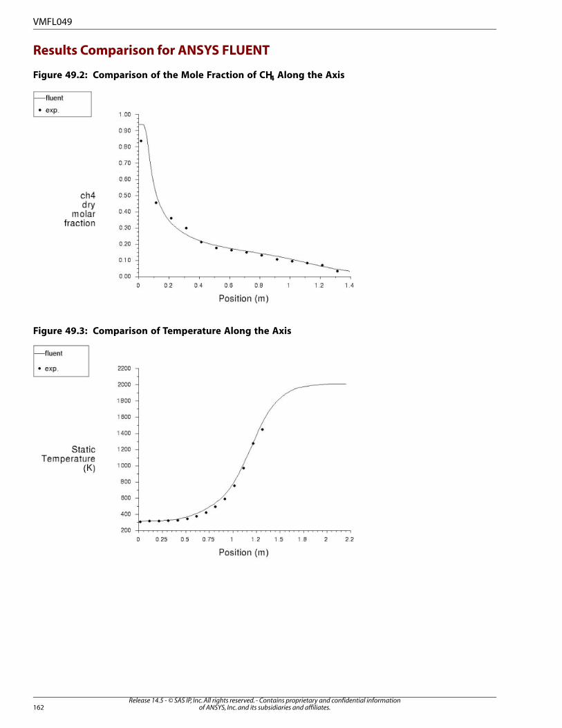
Results Comparison for ANSYS FLUENT
Figure 49.2: Comparison of the Mole Fraction of CH4 Along the Axis
Figure 49.3: Comparison of Temperature Along the Axis
Release 14.5 - © SAS IP, Inc. All rights reserved. - Contains proprietary and confidential informationof ANSYS, Inc. and its subsidiaries and affiliates.162
VMFL049

Results Comparison for ANSYS CFX
Figure 49.4: Comparison of the Mole Fraction of CH4 Along the Axis
163Release 14.5 - © SAS IP, Inc. All rights reserved. - Contains proprietary and confidential information
of ANSYS, Inc. and its subsidiaries and affiliates.
VMFL049

Figure 49.5: Comparison of Temperature Along the Axis
Release 14.5 - © SAS IP, Inc. All rights reserved. - Contains proprietary and confidential informationof ANSYS, Inc. and its subsidiaries and affiliates.164
VMFL049

VMFL050: Transient Heat Conduction in a Semi-Infinite Slab
Overview
F.P. Incropera, D.P. Dewitt, T.L. Bergman, and A.S. Lavine, “Introduction to Heat
Transfer”, 5th Edition, Wiley & Sons, 2007; Page 283.
Reference
ANSYS FLUENT, ANSYS CFXSolver
Transient heat transfer, ConductionPhysics/Models
Input File VMFL050_FLUENT.cas for ANSYS FLUENT
VMFL050_CFX.def for ANSYS CFX
Test Case
Unsteady heat conduction in a thick copper plate is modeled. Initially (at t = 0) the plate is at a uniform
temperature of 293 K. It is suddenly exposed to a heat transfer at one surface with a constant heat flux
of 3 X 10⁵
W/m2. The temperature distribution after 2 minutes is considered for verification.
Figure 50.1: Flow Domain
Conduction
Heat Flux at T>0
Boundary ConditionsGeometryMaterial Properties
Heat Flux = 3 X 10⁵
W/m2 on one wall. The op-
posite wall is adiabatic.
Dimensions of
the slab:
Density = 8995.67
kg/m3
Specific Heat = 381
J/kg-K
Lateral boundaries are modeled as planes of
symmetry.
750 mm X
300 mm
Conductivity = 401
W/m-K
Analysis Assumptions and Modeling Notes
The flow is transient. The dimensions considered here are adequate for the semi-infinite slab assumption.
The domain is initialized with a uniform temperature of 293 K corresponding to the condition at time
= 0 sec.
165Release 14.5 - © SAS IP, Inc. All rights reserved. - Contains proprietary and confidential information
of ANSYS, Inc. and its subsidiaries and affiliates.

Results Comparison for ANSYS FLUENT
Table 50.1: Comparison of Temperature after 2 Minutes
RatioExact SolutionANSYS FLUENT
0.9998393 K392.95 KTemperature of the wall exposed
to heat flux, at t=120 sec
1.0000318.4 K318.41 KTemperature at a point 150 mm
from the heat flux wall, at t=120
sec
Results Comparison for ANSYS CFX
Table 50.2: Comparison of Temperature after 2 Minutes
Ra-
tio
Exact Solu-
tion
ANSYS
CFX
1.0000393 K393 KTemperature of the wall exposed to heat flux, at t=120 sec
1.0000318.4 K318.4 KTemperature at a point 150 mm from the heat flux wall, at t=120
sec
Release 14.5 - © SAS IP, Inc. All rights reserved. - Contains proprietary and confidential informationof ANSYS, Inc. and its subsidiaries and affiliates.166
VMFL050

VMFL051: Isentropic Expansion of Supersonic Flow over a Convex Corner
Overview
John Anderson. “Modern Compressible Flow: With Historical Perspective”.Reference
ANSYS FLUENT, ANSYS CFXSolver
Compressible, inviscid flowPhysics/Models
Input File VMFL051_FLUENT.cas for ANSYS FLUENT
VMFL051_CFX.def for ANSYS CFX
Test Case
Centered expansion of inviscid supersonic flow around a corner is modeled. The expansion results in a
change in direction of the flow, a drop in static pressure, and increase in Mach number. The approaching
flow is supersonic, with a Mach number of 2.5. The expansion process is reversible and adiabatic.
Figure 51.1: Flow Domain
Incoming ow, M>1
Flow after expansion, M>>1Ø = 195º
adiabatic wall
Boundary ConditionsGeometryMaterial Properties
Inlet:Angle round the
corner = 195°
Density: Ideal Gas law
Specific Heat = 1006.43
J/kg-K
Pressure = 202636.9 Pa
Mach number = 2.5,
Molecular weight =
28.966
Static temperature = 300 K (In CFX, the
corresponding velocity is specified).
Wall is adiabatic.
Analysis Assumptions and Modeling Notes
The flow is steady and compressible. Inviscid and incompressible. Analytic expressions for isentropic
expansion can be used to calculate the Mach number downstream of the corner.
167Release 14.5 - © SAS IP, Inc. All rights reserved. - Contains proprietary and confidential information
of ANSYS, Inc. and its subsidiaries and affiliates.

Results Comparison for ANSYS FLUENT
Table 51.1: Comparison of Mach Number Downstream of the Corner, after Expansion
Ra-
tio
Analytical Calcula-
tion
ANSYS FLU-
ENT
0.99803.23703.2316Mach number after expan-
sion
Results Comparison for ANSYS CFX
Table 51.2: Comparison of Mach Number Downstream of the Corner, after Expansion
Ra-
tio
Analytical Calcula-
tion
ANSYS
CFX
0.99903.23703.2340Mach number after expan-
sion
Release 14.5 - © SAS IP, Inc. All rights reserved. - Contains proprietary and confidential informationof ANSYS, Inc. and its subsidiaries and affiliates.168
VMFL051

VMFL052: Turbulent Natural Convection inside a Tall Cavity
Overview
P.L. Betts and I.H. Bokhari. "Experiments on turbulent natural convection in an
enclosed tall cavity". International Journal of Heat and Fluid Flow, 21. 675-683.
2000.
Reference
ANSYS FLUENT, ANSYS CFXSolver
Turbulent flow, buoyancy effects, Boussinesq approximation (FLUENT)/Ideal gas
(CFX)
Physics/Models
Input File VMFL052_FLUENT.cas for ANSYS FLUENT
VMFL052_CFX.def for ANSYS CFX
Test Case
Natural convection in the turbulent flow field of an enclosed cavity with a length-to-width ratio of 28.6
is modeled. The Rayleigh number is in the turbulent range. The two vertical walls are kept at different
temperatures, while the horizontal walls are adiabatic.
Figure 52.1: Flow Domain (not to scale)
Hot Wall
Cold Wall
g = 9.81m/sec2
169Release 14.5 - © SAS IP, Inc. All rights reserved. - Contains proprietary and confidential information
of ANSYS, Inc. and its subsidiaries and affiliates.

Boundary ConditionsGeometryMaterial Properties
Temperature of Cold wall =
288.25 K
Length of the cavity
= 2.18 m
Density : Boussinesq approximation
(FLUENT), Ideal Gas law (CFX)
Temperature of Hot wall =
307.85 K
Width of the cavity
= 0.0762 m
Specific Heat = 1005 J/kg-K
Viscosity = 1.81X 10⁻⁵
kg/m-secTop and bottom walls are
adiabaticMolecular weight = 28.966
Analysis Assumptions and Modeling Notes
The flow is steady and is induced by natural convective heat transfer.
Results Comparison for ANSYS FLUENT
Figure 52.2: Comparison of Vertical Velocity at Y/h = 0.05
Release 14.5 - © SAS IP, Inc. All rights reserved. - Contains proprietary and confidential informationof ANSYS, Inc. and its subsidiaries and affiliates.170
VMFL052

Figure 52.3: Comparison of Temperature at Y/h = 0.05
Results Comparison for ANSYS CFX
Figure 52.4: Comparison of Vertical Velocity at Y/h = 0.05
171Release 14.5 - © SAS IP, Inc. All rights reserved. - Contains proprietary and confidential information
of ANSYS, Inc. and its subsidiaries and affiliates.
VMFL052

Figure 52.5: Comparison of Temperature at Y/h = 0.05
Release 14.5 - © SAS IP, Inc. All rights reserved. - Contains proprietary and confidential informationof ANSYS, Inc. and its subsidiaries and affiliates.172
VMFL052

VMFL053: Compressible Turbulent Mixing Layer
Overview
S.G. Goebel and J.C. Dutton. “Experimental Study of Compressible Turbulent
Mixing Layers”. AIAA Journal, 29(4). 538-546. 1991.
Reference
ANSYS FLUENTSolver
Turbulence: RNG k-ε model, compressible, energy equationPhysics/Models
Input File VMFL053_FLUENT.cas for ANSYS FLUENT
Test Case
Two streams of air are mixed in a rectangular tunnel. The length of the computational domain is chosen
such that the local Reynolds number at the exit of the test section, which is based on the velocity dif-
ference between the streams and the mixing layer thickness, is greater than 100,000. This is the Reynolds
number needed for the complete development of the mixing layer.
Figure 38.1: Flow Domain
Symmetry
Outlet72 mm
Outlet
Symmetry
300 mm
Inlet
U_1 = 616 m/s
U_2 = 100 m/s
Boundary ConditionsGeometryMaterial Properties
Primary Stream (1):Dimensions of the
domain:
Air:
Total Pressure = 487 kPaDensity: Ideal Gas
300mm X 72 mmSpecific Heat: 1006.43
J/kg-K
Static Pressure = 36 kPa
Total Temperature = 360 K
Thermal Conductivity:
0.0242 W/m-K
Mach Number = 2.35
Turbulent Kinetic Energy =
74 m2/s
2Viscosity: 1.4399e-05
kg/m-s Turbulent Dissipation Rate
= 62,300 m2/s
3
Secondary Stream (2):
Total Pressure = 37.6 kPa
Static Pressure = 36 kPa
Total Temperature = 290 K
Mach Number = 0.36
173Release 14.5 - © SAS IP, Inc. All rights reserved. - Contains proprietary and confidential information
of ANSYS, Inc. and its subsidiaries and affiliates.

Boundary ConditionsGeometryMaterial Properties
Turbulent Kinetic Energy =
226 m2/s
2
Turbulent Dissipation Rate
= 332,000 m2/s
3
Analysis Assumptions and Modeling Notes
The flow is steady, turbulent, and compressible. The RNG k-ε model is used for turbulence.
Results Comparison
The velocity profiles as the mixing layer evolves are compared with the experimental data.
Figure 38.2: X Velocity Profiles at x = 50 mm
Release 14.5 - © SAS IP, Inc. All rights reserved. - Contains proprietary and confidential informationof ANSYS, Inc. and its subsidiaries and affiliates.174
VMFL053

VMFL054: Laminar flow in a Trapezoidal Cavity
Overview
J.H. Darr and S.P. Vanka. “Separated Flow in a Driven Trapezoidal Cavity”. Phys.
Fluids A, 3(3):385-392. March 1991.
Reference
ANSYS FLUENT, ANSYS CFXSolver
Viscous flow, driven by a moving wallsPhysics/Models
Input File VMFL054_FLUENT.cas for ANSYS FLUENT
VMFL054_CFX.def for ANSYS CFX
Test Case
Laminar flow induced by the motion of the top wall of a trapezoidal cavity. The top and bottom walls
move but the side walls are stationary. The height of the cavity h is 1 m. The widths of the top and
bottom walls are 1 m and 2 m, respectively (Figure 38.1: Flow Domain (p. 175)).
Figure 38.1: Flow Domain
U = 400 m/s
1m
wall
1m
2 mm
U = 400 m/swall
Boundary ConditionsGeometryMaterial Proper-
ties
Velocity of the base walls =
400 m/s
Height of cavity = 1 m
Width of the bottom base
= 2 m
Density = 1
kg/m3
Viscosity = 1
kg/m-s
Other walls are stationary
Width of the top base = 1
m
Analysis Assumptions and Modeling Notes
The flow is steady. A pressure based solver is used. A triangular mesh of 4016 cells is used to discretize
the domain.
175Release 14.5 - © SAS IP, Inc. All rights reserved. - Contains proprietary and confidential information
of ANSYS, Inc. and its subsidiaries and affiliates.

Results Comparison for ANSYS FLUENT
The u-velocity profile at the vertical centerline of the cavity and the ν-velocity profile at the horizontal
centerline of the cavity are compared to Darr and Vanka results. Velocity is normalized by velocity of
the moving wall.
Figure 38.2: Normalized v-Velocity at the Horizontal Centerline of the Cavity
Figure 38.3: Normalized u-Velocity at the Vertical Centerline of the Cavity
Results Comparison for ANSYS CFX
The u-velocity profile at the vertical centerline of the cavity and the ν-velocity profile at the horizontal
centerline of the cavity are compared to Darr and Vanka results. Velocity is normalized by velocity of
the moving wall.
Release 14.5 - © SAS IP, Inc. All rights reserved. - Contains proprietary and confidential informationof ANSYS, Inc. and its subsidiaries and affiliates.176
VMFL054
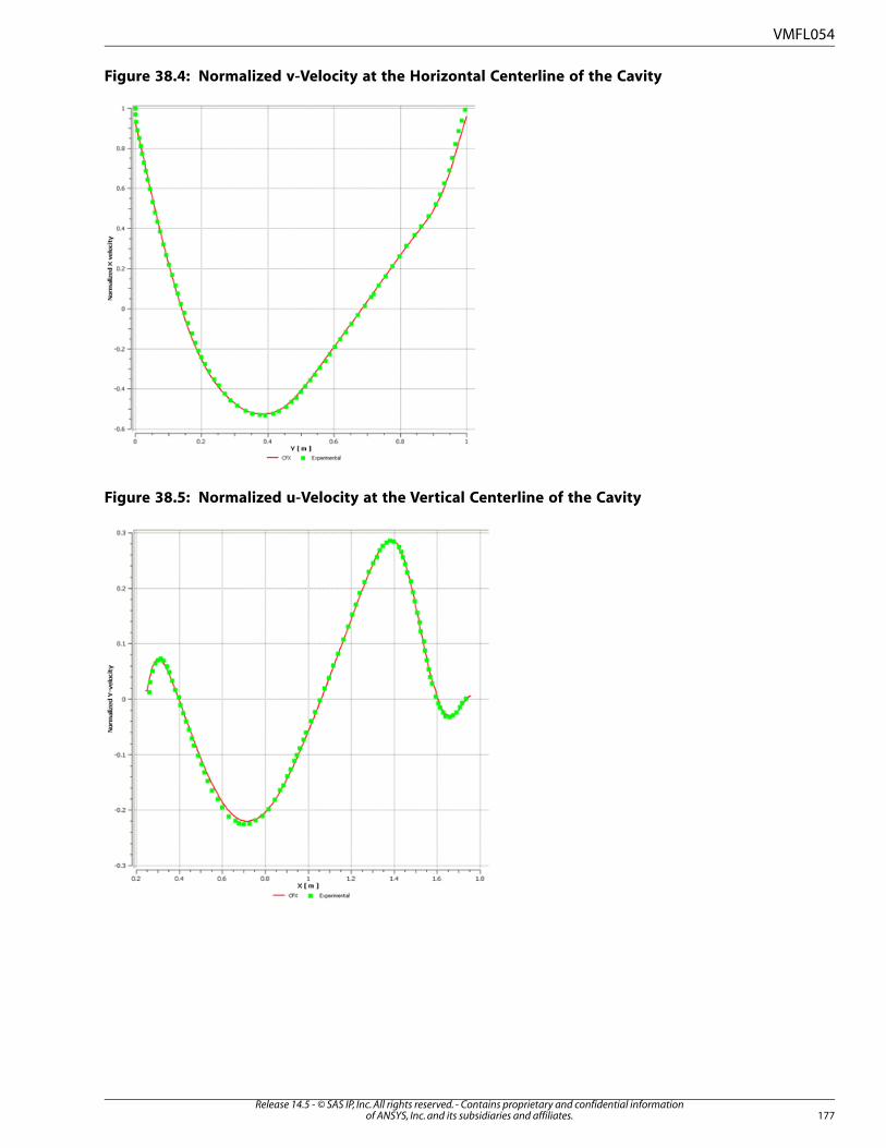
Figure 38.4: Normalized v-Velocity at the Horizontal Centerline of the Cavity
Figure 38.5: Normalized u-Velocity at the Vertical Centerline of the Cavity
177Release 14.5 - © SAS IP, Inc. All rights reserved. - Contains proprietary and confidential information
of ANSYS, Inc. and its subsidiaries and affiliates.
VMFL054

Release 14.5 - © SAS IP, Inc. All rights reserved. - Contains proprietary and confidential informationof ANSYS, Inc. and its subsidiaries and affiliates.178

VMFL055: Transitional Recirculatory Flow inside a Ventilation Enclosure
Overview
A. Restivo. Turbulent Flow in Ventilated Rooms. Ph.D. Thesis, University of
London, U.K. 1979.
Reference
ANSYS FLUENT, ANSYS CFXSolver
Transitional turbulence modeling (k-kl model for ANSYS FLUENT, BSL Gamma
Model for ANSYS CFX)
Physics/Models
Input File VMFL055_FLUENT.cas for ANSYS FLUENT
VMFL055_CFX-BSL-Gamma.def for ANSYS CFX
Test Case
Flow inside an enclosure similar to a ventilated room is modeled. The flow field is transitional and
dominated by recirculation. Reynolds number is based on the inlet dimension and is around 5000.
Figure 55.1: Flow Domain
H = 3m
Inlet
Outlet
Boundary ConditionsGeometryMaterial Properties
Inlet velocity =
0.45 m/S
Height of the enclosure (H) =
3 mDensity : 1.225 kg/m
3
Viscosity = 1.7894 X 10⁻⁵
kg/m-secLength of the enclosure = 9 m
(3 H)
Inlet : 0.056 H
Outlet : 0.16 H
Analysis Assumptions and Modeling Notes
The flow is modeled using transitional turbulence models.
179Release 14.5 - © SAS IP, Inc. All rights reserved. - Contains proprietary and confidential information
of ANSYS, Inc. and its subsidiaries and affiliates.

Results Comparison for ANSYS FLUENT
Figure 55.2: Comparison of X-Velocity Velocity at Y = 2.916 m
Results Comparison for ANSYS CFX
Figure 55.3: Comparison of X-Velocity Velocity at Y = 2.916 m
Release 14.5 - © SAS IP, Inc. All rights reserved. - Contains proprietary and confidential informationof ANSYS, Inc. and its subsidiaries and affiliates.180
VMFL055

VMFL056: Combined Conduction and Radiation in a Square Cavity
Overview
Daniel R. Rousse, Guillaume Gautier, and Jean-Francois Sacadura. “Numerical
predictions of two-dimensional conduction, convection, and radiation heat
Reference
transfer. II. Validation”. International Journal of Thermal Sciences. Volume 39,
Issue 3 (March 2000). 332-353.
ANSYS FLUENT, ANSYS CFXSolver
Radiation modeling; discrete ordinate model in ANSYS FLUENTPhysics/Models
Input File VMFL056_FLUENT.cas for ANSYS FLUENT
VMFL056_CFX.def for ANSYS CFX
Test Case
Coupled conduction and radiation is modeled in a square enclosure. The material properties are set to
model a condition corresponding to the Conduction-Radiation parameter N = 1.0. Scattering coefficient
of the medium is 0. Steady state heat transfer is modeled. One wall of the square cavity is kept at a
higher temperature than the other 3 walls.
Figure 56.1: Flow Domain
Hot Wall
Cold Walls
Boundary ConditionsGeometryMaterial Properties
Temperature of the hot wall =
100 K
Dimensions of the domain:
1 m X 1 m
Thermal Conductivity = 1
W/m-K
Temperature of the cold walls
= 50 K
Absorption Coefficient =
0.228/m
181Release 14.5 - © SAS IP, Inc. All rights reserved. - Contains proprietary and confidential information
of ANSYS, Inc. and its subsidiaries and affiliates.

Analysis Assumptions and Modeling Notes
The material properties are set to model the desired conduction-radiation fraction. Radiative heat flux
is only a small fraction of the total heat flux.
Results Comparison for ANSYS FLUENT
Figure 56.2: Comparison of Non-Dimensional Temperature at X = 0.5 m
Results Comparison for ANSYS CFX
Figure 56.3: Comparison of Non-Dimensional Temperature at X = 0.5 m
Release 14.5 - © SAS IP, Inc. All rights reserved. - Contains proprietary and confidential informationof ANSYS, Inc. and its subsidiaries and affiliates.182
VMFL056

VMFL057: Radiation and Conduction in Composite Solid Layers
Overview
C.M. Spuckler and R. Siegel. “Two-Flux and Diffusion Methods for Radiative
Transfer in Composite Layers”. J. Heat Transfer, 118. 218-222. 1996.
Reference
ANSYS FLUENTSolver
Radiation modeling with DO model, participating medium with gray-band
absorption
Physics/Models
Input File VMFL057_FLUENT.cas for ANSYS FLUENT
Test Case
Heat transfer by conduction and radiation is modeled in a composite solid domain consisting of two
layers. Both the layers participate in radiation. The two layers are separated by a semi-transparent wall.
The upstream and downstream sides of the domain are subjected to convective as well as radiative
heat transfer.
Figure 57.1: Flow Domain
Wall
Symmetry
Symmetry
WallSolid
1
Solid 2
Boundary ConditionsGeometryMaterial Properties
Left-most wall:Dimensions of the do-
main: 2 m X 1 m (the
Solid 1:
Density = 2719 kg/m3 Convectivetwo solid zones are of
equal length) Heat Transfer Coefficient =
56.7 W/m2 K
Specific Heat = 871 J/kg-k
Thermal Conductivity =
5.67 W/m-K free stream temperature =
1000KAbsorption Coefficient:
gray-band Semi-transparent
Right-most wall:Refractive Index = 1.5
Solid 2:Convective
Density = 2719 kg/m3 Heat Transfer Coefficient =
56.7 W/m2 KSpecific Heat = 871 J/kg-k
183Release 14.5 - © SAS IP, Inc. All rights reserved. - Contains proprietary and confidential information
of ANSYS, Inc. and its subsidiaries and affiliates.

Boundary ConditionsGeometryMaterial Properties
free stream temperature =
250K
Thermal Conductivity =
5.67 W/m-K
Semi-transparentAbsorption Coefficient:
gray-band
Refractive Index = 3
Analysis Assumptions and Modeling Notes
Transverse boundaries of the domain are modeled as planes of symmetry.
Results Comparison for ANSYS FLUENT
Figure 57.2: Comparison temperature distribution along Y = 0.5 m
Release 14.5 - © SAS IP, Inc. All rights reserved. - Contains proprietary and confidential informationof ANSYS, Inc. and its subsidiaries and affiliates.184
VMFL057
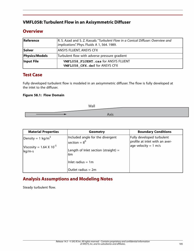
VMFL058: Turbulent Flow in an Axisymmetric Diffuser
Overview
R. S. Azad and S. Z. Kassab. “Turbulent Flow in a Conical Diffuser: Overview and
implications”. Phys. Fluids A 1, 564. 1989.
Reference
ANSYS FLUENT, ANSYS CFXSolver
Turbulent flow with adverse pressure gradientPhysics/Models
Input File VMFL058_FLUENT.cas for ANSYS FLUENT
VMFL058_CFX.def for ANSYS CFX
Test Case
Fully developed turbulent flow is modeled in an axisymmetric diffuser. The flow is fully developed at
the inlet to the diffuser.
Figure 58.1: Flow Domain
Axis
Wall
Boundary ConditionsGeometryMaterial Properties
Fully developed turbulent
profile at inlet with an aver-
age velocity = 1 m/s
Included angle for the divergent
section = 80
Length of Inlet section (straight) =
6m
Density = 1 kg/m3
Viscosity = 1.64 X 10⁻⁵
kg/m-s
Inlet radius = 1m
Outlet radius = 2m
Analysis Assumptions and Modeling Notes
Steady turbulent flow.
185Release 14.5 - © SAS IP, Inc. All rights reserved. - Contains proprietary and confidential information
of ANSYS, Inc. and its subsidiaries and affiliates.
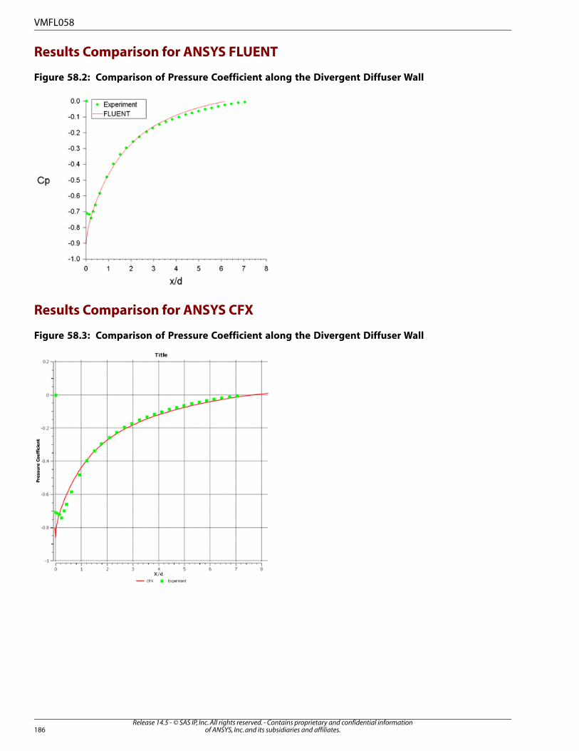
Results Comparison for ANSYS FLUENT
Figure 58.2: Comparison of Pressure Coefficient along the Divergent Diffuser Wall
Results Comparison for ANSYS CFX
Figure 58.3: Comparison of Pressure Coefficient along the Divergent Diffuser Wall
Release 14.5 - © SAS IP, Inc. All rights reserved. - Contains proprietary and confidential informationof ANSYS, Inc. and its subsidiaries and affiliates.186
VMFL058
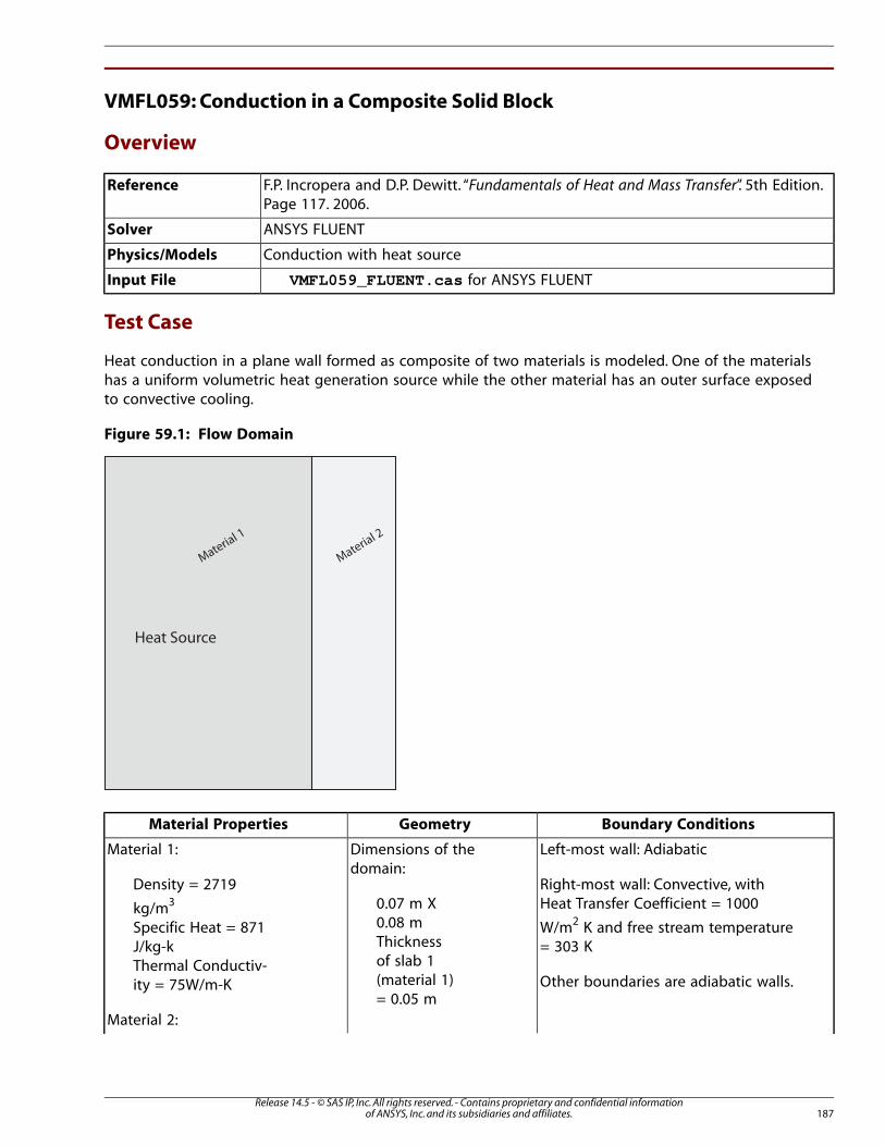
VMFL059: Conduction in a Composite Solid Block
Overview
F.P. Incropera and D.P. Dewitt. “Fundamentals of Heat and Mass Transfer”. 5th Edition.
Page 117. 2006.
Reference
ANSYS FLUENTSolver
Conduction with heat sourcePhysics/Models
Input File VMFL059_FLUENT.cas for ANSYS FLUENT
Test Case
Heat conduction in a plane wall formed as composite of two materials is modeled. One of the materials
has a uniform volumetric heat generation source while the other material has an outer surface exposed
to convective cooling.
Figure 59.1: Flow Domain
Material 1
Material 2
Heat Source
Boundary ConditionsGeometryMaterial Properties
Left-most wall: AdiabaticDimensions of the
domain:
Material 1:
Right-most wall: Convective, with
Heat Transfer Coefficient = 1000
Density = 2719
kg/m3 0.07 m X
0.08 m W/m2 K and free stream temperature
= 303 K
Specific Heat = 871
J/kg-k Thickness
of slab 1
Other boundaries are adiabatic walls.Thermal Conductiv-
ity = 75W/m-K (material 1)
= 0.05 m
Material 2:
187Release 14.5 - © SAS IP, Inc. All rights reserved. - Contains proprietary and confidential information
of ANSYS, Inc. and its subsidiaries and affiliates.

Boundary ConditionsGeometryMaterial Properties
Density = 8978
kg/m3
Specific Heat = 381
J/kg-k
Thermal Conductiv-
ity = 150 W/m-K
Analysis Assumptions and Modeling Notes
Contact resistance between the slabs is neglected.
Results Comparison
Table 59.1: Comparison Temperatures on the Side Walls
Ra-
tio
Analytic-
al
ANSYS FLU-
ENT
1.0004378 K378.16 KTemperature of the cooled wall
1.0003413 K413.12 KTemperature of the adiabatic wall on extreme left
side
Release 14.5 - © SAS IP, Inc. All rights reserved. - Contains proprietary and confidential informationof ANSYS, Inc. and its subsidiaries and affiliates.188
VMFL059

VMFL060: Transitional Supersonic Flow over a Rearward Facing Step
Overview
Howard E Smith. “The Flow Field and Heat Transfer downstream of a Rearward
Facing Step in Supersonic Flow”. ARL 67-0056, Aerospace Research Laboratories.
Ohio, USA.
Reference
ANSYS FLUENT, ANSYS CFXSolver
Compressible Flow, Transitional turbulence modeling (Transition SST model
for ANSYS FLUENT, SST Gamma-Theta Model for ANSYS CFX)
Physics/Models
Input File VMFL060_FLUENT.cas for ANSYS FLUENT
VMFL060_CFX.def for ANSYS CFX
Test Case
Supersonic flow with an inlet Mach number 2.5 past a backward facing step is modeled. Key features
of the flow field include sudden expansion, free shear layer, recirculation zone, and oblique shock.
Reynolds number of the flow (based on step height) is in the transitional range.
Figure 60.1: Flow Domain
Traverse boundary
Supersonic Flow (M = 2.5)
Step (h = 0.443”)
Boundary ConditionsGeometryMaterial Properties
Total pressure at inlet = 227527 PaStep Height = 0.443 inDensity: Ideal gas
Static Pressure at Inlet = 13316.6Inlet: 4 in upstream of the
step
Viscosity = 1.7894
X 10-5
kg/m-secTotal temperature at inlet = 344.44 K
Outlet: 12 in downstream of
the step Transverse boundary modeled as far-
field (ANSYS FLUENT)/ Supersonic outlet
(ANSYS CFX)Transverse (top) boundary:
6.25 in above the step.Walls are modeled as adiabatic
Analysis Assumptions and Modeling Notes
The flow is modeled using transitional turbulence models.
189Release 14.5 - © SAS IP, Inc. All rights reserved. - Contains proprietary and confidential information
of ANSYS, Inc. and its subsidiaries and affiliates.

Results Comparison for ANSYS FLUENT
Figure 60.2: Comparison of Non-Dimensionalized Static Pressure along the Stepped Wall
Downstream of the Corner
Results Comparison for ANSYS CFX
Figure 60.3: Comparison of Non-Dimensionalized Static Pressure along the Stepped Wall
Downstream of the Corner
Release 14.5 - © SAS IP, Inc. All rights reserved. - Contains proprietary and confidential informationof ANSYS, Inc. and its subsidiaries and affiliates.190
VMFL060

VMFL061: Surface to Surface Radiative Heat Transfer between Two Concentric
Cylinders
Overview
F.P. Incropera and D.P. Dewitt. “Fundamentals of Heat and Mass Transfer”. 4th
Edition. New York City, New York: John Wiley & Sons, Inc. 1996.
Reference
ANSYS FLUENT, ANSYS CFXSolver
Radiation Modeling (S2S Model in ANSYS FLUENT, Monte Carlo Method in ANSYS
CFX)
Physics/Models
Input File VMFL061_FLUENT.cas for ANSYS FLUENT
VMFL061_CFX.def for ANSYS CFX
Test Case
Radiative heat transfer between two cylindrical surfaces forming a concentric annulus is modeled. There
is no participating medium. Due to symmetry only the shaded portion of the domain in Figure 61.1: Flow
Domain (p. 191) is modeled.
Figure 61.1: Flow Domain
Cold outer wall
Hot inner
wall
Boundary ConditionsGeometryMaterial Properties
Temperature of inner wall =
700 K
Radius of inner wall =
0.04625 m
Material does not participate in the
energy transfer.
191Release 14.5 - © SAS IP, Inc. All rights reserved. - Contains proprietary and confidential information
of ANSYS, Inc. and its subsidiaries and affiliates.

Boundary ConditionsGeometryMaterial Properties
Temperature of outer wall
= 300 K
Radius of outer wall =
0.0178 m
Analysis Assumptions and Modeling Notes
Because there is no flow of mass, only the energy equation is solved. Radiation models are used for the
simulation. Heat transfer is purely due to radiation between the two surfaces.
Results Comparison for ANSYS FLUENT
Figure 61.2: Comparison of Temperature Variation along Radius
Release 14.5 - © SAS IP, Inc. All rights reserved. - Contains proprietary and confidential informationof ANSYS, Inc. and its subsidiaries and affiliates.192
VMFL061

Results Comparison for ANSYS CFX
Figure 61.3: Comparison of Temperature Variation along Radius
193Release 14.5 - © SAS IP, Inc. All rights reserved. - Contains proprietary and confidential information
of ANSYS, Inc. and its subsidiaries and affiliates.
VMFL061

Release 14.5 - © SAS IP, Inc. All rights reserved. - Contains proprietary and confidential informationof ANSYS, Inc. and its subsidiaries and affiliates.194

VMFL062: Fully Developed Turbulent Flow Over a “Hill”
Overview
V. Baskaran, A. J. Smits, and P. N. Joubert. "A turbulent flow over a curved hill Part
1. Growth of an internal boundary layer". Journal of Fluid Mechanics, (1987), 182: 47-
83.
Reference
ANSYS FLUENT, ANSYS CFXSolver
Low Re k-e Model in ANSYS FLUENT, k-e Model in ANSYS CFXPhysics/Models
Input File VMFL062_FLUENT.cas for ANSYS FLUENT
VMFL062_CFX.def for ANSYS CFX
Test Case
Flow over a “hill” geometry with separation and reattachment is modeled. Fully developed turbulent
profile is specified at the inlet.
Figure 62.1: Flow Domain
Hill
Flow Direction
Boundary ConditionsGeometryMaterial Properties
Fully developed profiles are specified at the
inlet for (i) Velocity, (ii) Turbulent kinetic En-
ergy, and (iii) Eddy dissipation rate.
Height of the hill
= 20.5 mmDensity : 1 kg/m
3
Viscosity = 7.5188e-07
kg/m-sAverage velocity at inlet = 1 m/s
195Release 14.5 - © SAS IP, Inc. All rights reserved. - Contains proprietary and confidential information
of ANSYS, Inc. and its subsidiaries and affiliates.

Results Comparison for ANSYS FLUENT
Figure 62.2: Comparison of Skin Friction along the Wall
Results Comparison for ANSYS CFX
Figure 62.3: Comparison of Skin Friction along the Wall
Release 14.5 - © SAS IP, Inc. All rights reserved. - Contains proprietary and confidential informationof ANSYS, Inc. and its subsidiaries and affiliates.196
VMFL062

VMFL063: Separated Laminar Flow over a Blunt Plate
Overview
J.C . Lane and R.I. Loehrke. “Leading Edge Separation from a Blunt Plate at Low
Reynolds Number”. Transactions of ASME, Volume 102 (December 1980): 494-
496.
Reference
ANSYS FLUENT, ANSYS CFXSolver
Laminar flow, high resolution numerical modelsPhysics/Models
Input File VMFL063_FLUENT.cas for ANSYS FLUENT
VMFL063_CFX.def for ANSYS CFX
Test Case
The flow separation over a blunt leading edge in laminar flow is modeled. The flow separates and
reattaches along the plate. The reattachment length predicted by the solvers is validated against exper-
imental results. Due to symmetry, only half of the domain shown in Figure 63.1: Flow Domain (p. 197)
is modeled. The Reynolds number based on plate thickness is 227.
Figure 63.1: Flow Domain
Plane of SymmetryReattachment
Blunt plate
Flow Direction
Boundary ConditionsGeometryMaterial Properties
Velocity at inlet = 0.045133
m/s
Thickness of the plate, 2t =
90 mmDensity: 1 kg/m
3
Viscosity: 1.7894 X 10⁻⁵
kg/m-sLength of the plate = 1500
mm
197Release 14.5 - © SAS IP, Inc. All rights reserved. - Contains proprietary and confidential information
of ANSYS, Inc. and its subsidiaries and affiliates.
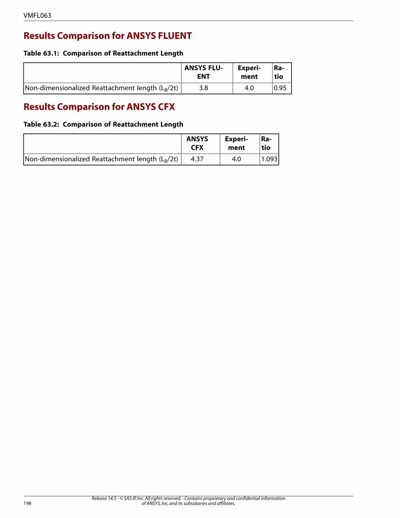
Results Comparison for ANSYS FLUENT
Table 63.1: Comparison of Reattachment Length
Ra-
tio
Experi-
ment
ANSYS FLU-
ENT
0.954.03.8Non-dimensionalized Reattachment length (LR/2t)
Results Comparison for ANSYS CFX
Table 63.2: Comparison of Reattachment Length
Ra-
tio
Experi-
ment
ANSYS
CFX
1.0934.04.37Non-dimensionalized Reattachment length (LR/2t)
Release 14.5 - © SAS IP, Inc. All rights reserved. - Contains proprietary and confidential informationof ANSYS, Inc. and its subsidiaries and affiliates.198
VMFL063

VMFL064: Low Reynolds Number Flow in a Channel with Sudden Asymmetric
Expansion
Overview
Reference 1. B. Armaly, F. Durst, J. Pereira, and B. Schönung. “Experimental and theoretical
investigation of a backward-facing step”. J. Fluid Mech. 127 (1983): 473.
2. C.J. Freitas. “Perspective: Selected Benchmarks from Commercial CFD Codes”. J.
Fluids Eng. Volume 117, Issue 2 (June 1995): 208.
ANSYS FLUENTSolver
Laminar flow, Separation, and ReattachmentPhysics/Models
Input File VMFL064_FLUENT.cas for ANSYS FLUENT
Test Case
Laminar flow in a channel with a backward facing step expansion is modeled. The channels section
upstream of the expansion is long enough to ensure fully developed laminar profile. The reattachment
length predicted by the solvers is validated against experimental results. Reynolds number based on D
(equal to twice the channel height at inlet) is 200. The domain extends to about 40 times the step-
height upstream and over 20 times the step-height downstream.
Figure 64.1: Flow Domain
Flow Direction
Boundary ConditionsGeometryMaterial Properties
Velocity at inlet =
0.288462 m/s
Step height, s = 4.9 mm
Channel height at inlet = 5.2 mm
Density: 1 kg/m3
Viscosity: 1.5 X 10⁻⁵
kg/m-sNo-slip condition at the
wallsLength of inlet section = 200 mm
Length downstream of the step =
100 mm
Analysis Assumptions and Modeling Notes
The flow is fully developed before the step. Reattachment length is measured from the reversal of the
sign of the wall shear along the flow direction.
199Release 14.5 - © SAS IP, Inc. All rights reserved. - Contains proprietary and confidential information
of ANSYS, Inc. and its subsidiaries and affiliates.

Results Comparison for ANSYS FLUENT
Table 64.1: Comparison of Reattachment Length
Ra-
tio
Experi-
ment
ANSYS FLU-
ENT
0.9865.04.93Non-dimensionalized Reattachment length (LR/Step-height)
Results Comparison for ANSYS CFX
Table 64.2: Comparison of Reattachment Length
Ra-
tio
Experi-
ment
ANSYS
CFX
0.985.04.90Non-dimensionalized Reattachment length (LR/Step-height)
Release 14.5 - © SAS IP, Inc. All rights reserved. - Contains proprietary and confidential informationof ANSYS, Inc. and its subsidiaries and affiliates.200
VMFL064

VMFL065: Swirling Turbulent Flow Inside a Diffuser
Overview
P.D. Clausen, S.G. Koh, and D.H. Wood. “Measurements of a Swirling Turbulent
Boundary Layer Developing in a Conical Diffuser.” Experimental Thermal and Fluid
Science. Volume 6, Issue 1 (January 1993): 39-48.
Reference
ANSYS FLUENTSolver
Turbulent flow, swirl velocity, Reynolds stress model for turbulencePhysics/Models
Input File VMFL065_FLUENT.cas for ANSYS FLUENT
Test Case
Turbulent flow with a strong swirl component is modeled in an axisysmmetric diffuser. The swirl com-
ponent of the velocity has a dominant effect on the flow field inside the diffuser.
Figure 65.1: Flow Domain
Flow
Boundary ConditionsGeometryMaterial Properties
Fully developed turbulent profile
for velocity, k and ε at inlet (with
Length of the straight inlet sec-
tion = 25 mmDensity: 1 kg/m
3
Viscosity: 1.293 X
10-6
kg/m-s
average axial inlet velocity = 1
m/s)
No-slip condition at the walls
Length of the diffuser (divergent
section) = 510 mm
Inlet Diameter = 260 mm
Outlet Diameter = 440 mm
Analysis Assumptions and Modeling Notes
RS model is used for turbulence due to the strong swirl component.
201Release 14.5 - © SAS IP, Inc. All rights reserved. - Contains proprietary and confidential information
of ANSYS, Inc. and its subsidiaries and affiliates.

Results Comparison for ANSYS FLUENT
Figure 65.2: Comparison of Swirl Velocity at X = 0.175 m
Release 14.5 - © SAS IP, Inc. All rights reserved. - Contains proprietary and confidential informationof ANSYS, Inc. and its subsidiaries and affiliates.202
VMFL065

VMFL066: Radiative Heat Transfer in a Rectangular Enclosure with Participating
Medium
Overview
G.D Raithby and E.H. Chui. “A Finite Volume Method for Predicting a Radiant
Heat Transfer in Enclosoures with Participating Media”. Journal of Heat Transfer.
Volume 112 (May 1990): 415-423.
Reference
ANSYS FLUENTSolver
Radiation modeling, discrete Ordinate Model in ANSYS FLUENTPhysics/Models
Input File VMFL066_FLUENT.cas for ANSYS FLUENT
Test Case
Two dimensional radiative heat transfer in an enclosure with one hot wall and three cold walls at equal
temperature is modeled. The enclosure is a rectangular cavity with a length-to-width ratio of 5. For the
problem being considered, σsLy = 1.0, where σ
s is the scattering coefficient and Ly is the normal distance
between the hot wall and the cold wall opposite to it.
Figure 66.1: Flow Domain
Hot Wall
Cold Walls
Boundary ConditionsGeometryMaterial Properties
Temperature of the hot wall =
200 K
Dimensions of the domain: 10
m x 2 m
Scattering coefficient =
0.5/m
Temperature of he cold walls
= 100 K
Analysis Assumptions and Modeling Notes
Isotropic scattering and radiative equilibrium are assumed.
203Release 14.5 - © SAS IP, Inc. All rights reserved. - Contains proprietary and confidential information
of ANSYS, Inc. and its subsidiaries and affiliates.

Results Comparison for ANSYS FLUENT
Figure 66.2: Comparison of Non-Dimensional Heat Flux along the Hot Wall
Release 14.5 - © SAS IP, Inc. All rights reserved. - Contains proprietary and confidential informationof ANSYS, Inc. and its subsidiaries and affiliates.204
VMFL066

VMFL067: Boiling in a Pipe-Critical Heat Flux
Overview
“Calculation of Dryout and Post-Dryout Heat Transfer for Tube Geometry”.
Norbert Hoyer Int. J. Multiphase Flow. Vol.24, No.2, pp. 319-334, 1998.
Reference
ANSYS FLUENTSolver
Multiphase, heat and mass transfer, boilingPhysics/Models
Input File VMFL067_FLUENT.cas for ANSYS FLUENT
Test Case
This test case considers boiling near a heated wall of a vertical pipe. The effects of critical heat flux and
post-dryout heat transfer are modeled in a vertical circular pipe. The outer wall of the pipe is heated
with a constant heat flux.
Figure 67.1: Flow Domain
Boundary ConditionsGeometryMaterial Properties
Mass flux at inlet = 1495 kg/m2/sRadius of the pipe =
5 mm
Steam-Water 2-phase
Flow:
Heat transfer at the wall = 797000
W/m2Height of the pipe =
7 m
• Water: continuous
phase
• Water Steam: dispersed
bubbles
205Release 14.5 - © SAS IP, Inc. All rights reserved. - Contains proprietary and confidential information
of ANSYS, Inc. and its subsidiaries and affiliates.

Analysis Assumptions and Modeling Notes
The flow is steady. RNG k-epsilon model is used for turbulence.
Results Comparison for ANSYS FLUENT
Figure 67.2: Comparison of Wall Temperature
Release 14.5 - © SAS IP, Inc. All rights reserved. - Contains proprietary and confidential informationof ANSYS, Inc. and its subsidiaries and affiliates.206
VMFL067

VMFL068: Axial Flow in an Eccentric Annulus
Overview
Simulated Velocity Profiles for Eccentric Annular Flow with Inner RotationReference
J.L. Vieira Neto 1, A.L. Martins3 , A. Silveira Neto2, C.H. Ataíde1, M.A.S. Barrozo1*
1. Federal University of Uberlândia, Chemical Engineering School,
Uberlândia, MG, Brazil.
2. Federal University of Uberlândia, Mechanical Engineering School,
Uberlândia, MG, Brazil.
3. PETROBRAS/CENPES/TEP, Rio de Janeiro, RJ, Brazil.
ANSYS FLUENTSolver
Steady flow, periodic, turbulence, RSMPhysics/Models
Input File VMFL068_FLUENT.cas for ANSYS FLUENT
Test Case
This test case considers axial flow in an eccentric annulus without rotation of the inner cylinder. Eccent-
ricity of the channel is 0.5. The Reynolds number is 26,600.
Figure 68.1: Flow Domain
Boundary ConditionsGeometryMaterial Properties
Periodic Boundary is used with
a Mass Flow Rate =1.8368 kg/s.
Diameter, outer cylinder =
40.3 mmDensity = 896 kg/m
3
Viscosity = 0.00146048
kg/m-s Diameter, inner cylinder =
20.1 mm
207Release 14.5 - © SAS IP, Inc. All rights reserved. - Contains proprietary and confidential information
of ANSYS, Inc. and its subsidiaries and affiliates.

Boundary ConditionsGeometryMaterial Properties
Eccentricity = 0.5
Analysis Assumptions and Modeling Notes
The flow is steady. The velocity profile at the inlet is fully developed.
Results Comparison for ANSYS FLUENT
Figure 68.2: Comparison of Normalized Axial Velocity at Plane 2
Figure 68.3: Comparison of Normalized Axial Velocity at Plane 3
Release 14.5 - © SAS IP, Inc. All rights reserved. - Contains proprietary and confidential informationof ANSYS, Inc. and its subsidiaries and affiliates.208
VMFL068

VMFL069: Two Phase Poiseulle Flow
Overview
Marchandise, Emilie and Remacle, Jean-Fancois. A Stabilized Finite Element
Method using a Discontinuous Level Set Approach for Solving Two Phase Incom-
pressible Flows.
Reference
ANSYS FLUENTSolver
Steady flow, laminar, two phase, vofPhysics/Models
Input File VMFL069_FLUENT.cas for ANSYS FLUENT
Test Case
This test case considers the horizontal stratified Poiseulle flow of two fluids between parallel walls. The
interface between the two phases is located at half of the height of the channel.
Figure 69.1: Flow Domain
Boundary ConditionsGeometryMaterial Properties
Periodic Boundary is used with
a Pressure Gradient =-0.5 Pa/m.
Dimensions of the
domain: 2 m X 4 m
The two fluids have the same
density.
Kinematic Viscosity
Fluid-1 = 0.1
Fluid-2 = 0.02
Analysis Assumptions and Modeling Notes
The flow is steady. Deformation of the interface is not modeled.
209Release 14.5 - © SAS IP, Inc. All rights reserved. - Contains proprietary and confidential information
of ANSYS, Inc. and its subsidiaries and affiliates.

Results Comparison for ANSYS FLUENT
Figure 69.2: Comparison of Velocity Profile for Two Phase Flow
Release 14.5 - © SAS IP, Inc. All rights reserved. - Contains proprietary and confidential informationof ANSYS, Inc. and its subsidiaries and affiliates.210
VMFL069

VMFL070: Radiation Between Two Parallel Surfaces
Overview
F.P. Incropera and D.P. Dewitt. Fundamentals of Heat and Mass Transfer. 4th
Edition. New York City, New York: John Wiley & Sons, Inc. 1996.
Reference
ANSYS FLUENTSolver
Heat Transfer, radiationPhysics/Models
Input File VMFL070_FLUENT.cas for ANSYS FLUENT
Test Case
This test case considers radiation heat transfer between two parallel surfaces. The surfaces are modeled
as a rectangle with a length-to-gap aspect ratio of 5 to minimize the edge effect near the mid span.
The gap thickness between the upper and lower surfaces is 0.5 m.
Figure 70.1: Flow Domain
Boundary ConditionsGeometryMaterial Properties
Top Wall Temperature =
400K
Dimensions of the do-
main: 5 m X 0.5 m
Material does not participate in
the energy transfer.
Bottom Wall Temperature
= 300K
Analysis Assumptions and Modeling Notes
Because there is no flow of mass, only the energy equation is solved. Heat transfer is purely due to ra-
diation between the two surfaces.
211Release 14.5 - © SAS IP, Inc. All rights reserved. - Contains proprietary and confidential information
of ANSYS, Inc. and its subsidiaries and affiliates.

Results Comparison for ANSYS FLUENT
Figure 70.2: Comparison of Normalized Temperature with Analytical Result
Release 14.5 - © SAS IP, Inc. All rights reserved. - Contains proprietary and confidential informationof ANSYS, Inc. and its subsidiaries and affiliates.212
VMFL070