Tutorial 21. Using the Eulerian Multiphase Model for Granular …barbertj/CFD Training/Fluent 12/t… · · 2009-10-07Using the Eulerian Multiphase Model for ... Use FLUENT Launcher

Tutorial 21. Using the Eulerian Multiphase Model forGranular Flow

Introduction

Mixing tanks are used to maintain solid particles or droplets of heavy fluids in suspension.Mixing may be required to enhance reaction during chemical processing or to preventsedimentation. In this tutorial, you will use the Eulerian multiphase model to solve theparticle suspension problem. The Eulerian multiphase model solves momentum equationsfor each of the phases, which are allowed to mix in any proportion.

This tutorial demonstrates how to do the following:

• Use the granular Eulerian multiphase model.

• Specify fixed velocities with a user-defined function (UDF) to simulate an impeller.

• Set boundary conditions for internal flow.

• Calculate a solution using the pressure-based solver.

• Solve a time-accurate transient problem.

Prerequisites

This tutorial is written with the assumption that you have completed Tutorial 1, andthat you are familiar with the ANSYS FLUENT navigation pane and menu structure.Some steps in the setup and solution procedure will not be shown explicitly.

Problem Description

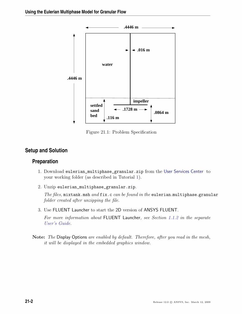
The problem involves the transient startup of an impeller-driven mixing tank. Theprimary phase is water, while the secondary phase consists of sand particles with a 111micron diameter. The sand is initially settled at the bottom of the tank, to a level justabove the impeller. A schematic of the mixing tank and the initial sand position is shownin Figure 21.1. The domain is modeled as 2D axisymmetric.

The fixed-values option will be used to simulate the impeller. Experimental data are usedto represent the time-averaged velocity and turbulence values at the impeller location.This approach avoids the need to model the impeller itself. These experimental data areprovided in a user-defined function.

Release 12.0 c© ANSYS, Inc. March 12, 2009 21-1

Using the Eulerian Multiphase Model for Granular Flow

.4446 m

.4446 m

water

settledsandbed

impeller

.1728 m

.116 m.0864 m

.016 m

Figure 21.1: Problem Specification

Setup and Solution

Preparation

1. Download eulerian_multiphase_granular.zip from the User Services Center toyour working folder (as described in Tutorial 1).

2. Unzip eulerian_multiphase_granular.zip.

The files, mixtank.msh and fix.c can be found in the eulerian multiphase granular

folder created after unzipping the file.

3. Use FLUENT Launcher to start the 2D version of ANSYS FLUENT.

For more information about FLUENT Launcher, see Section 1.1.2 in the separateUser’s Guide.

Note: The Display Options are enabled by default. Therefore, after you read in the mesh,it will be displayed in the embedded graphics window.

21-2 Release 12.0 c© ANSYS, Inc. March 12, 2009

http://www.fluentusers.com


Step 1: Mesh

1. Read the mesh file mixtank.msh.

File −→ Read −→Mesh...

A warning message will be displayed twice in the console. You need not take anyaction at this point, as the issue will be rectified when you define the solver settingsin Step 2.

Step 2: General Settings

General

1. Check the mesh.

General −→ Check

ANSYS FLUENT will perform various checks on the mesh and report the progressin the console. Ensure hat the reported minimum volume is a positive number.

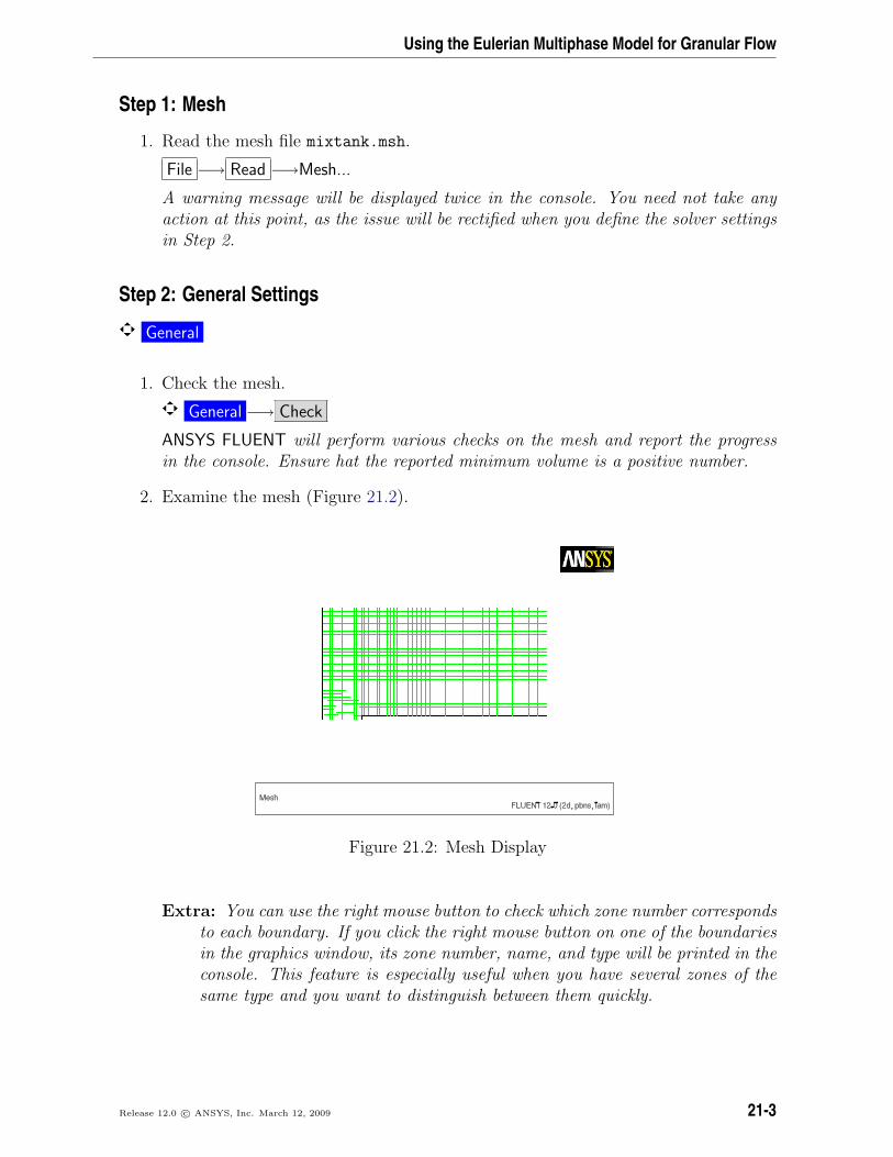
2. Examine the mesh (Figure 21.2).

Figure 21.2: Mesh Display

Extra: You can use the right mouse button to check which zone number correspondsto each boundary. If you click the right mouse button on one of the boundariesin the graphics window, its zone number, name, and type will be printed in theconsole. This feature is especially useful when you have several zones of thesame type and you want to distinguish between them quickly.



3. Modify the mesh colors.

General −→ Display...

(a) Click the Colors... button to open the Mesh Colors dialog box.

You can control the colors used to draw meshes by using the options availablein the Mesh Colors dialog box.

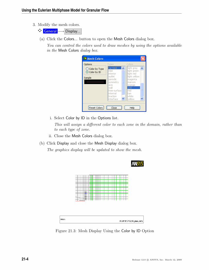
i. Select Color by ID in the Options list.

This will assign a different color to each zone in the domain, rather thanto each type of zone.

ii. Close the Mesh Colors dialog box.

(b) Click Display and close the Mesh Display dialog box.

The graphics display will be updated to show the mesh.

Figure 21.3: Mesh Display Using the Color by ID Option



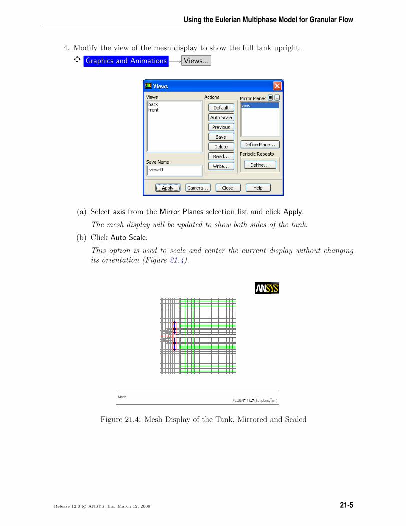
4. Modify the view of the mesh display to show the full tank upright.

Graphics and Animations −→ Views...

(a) Select axis from the Mirror Planes selection list and click Apply.

The mesh display will be updated to show both sides of the tank.

(b) Click Auto Scale.

This option is used to scale and center the current display without changingits orientation (Figure 21.4).

Figure 21.4: Mesh Display of the Tank, Mirrored and Scaled



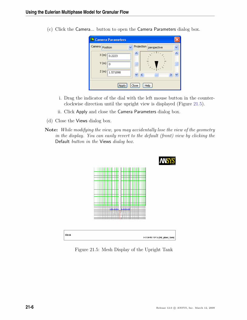
(c) Click the Camera... button to open the Camera Parameters dialog box.

i. Drag the indicator of the dial with the left mouse button in the counter-clockwise direction until the upright view is displayed (Figure 21.5).

ii. Click Apply and close the Camera Parameters dialog box.

(d) Close the Views dialog box.

Note: While modifying the view, you may accidentally lose the view of the geometryin the display. You can easily revert to the default (front) view by clicking theDefault button in the Views dialog box.

Figure 21.5: Mesh Display of the Upright Tank



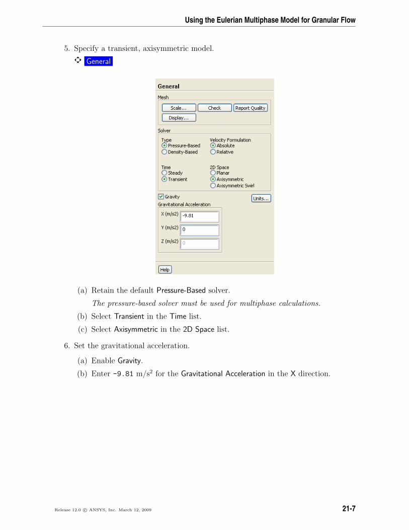
5. Specify a transient, axisymmetric model.

General

(a) Retain the default Pressure-Based solver.

The pressure-based solver must be used for multiphase calculations.

(b) Select Transient in the Time list.

(c) Select Axisymmetric in the 2D Space list.

6. Set the gravitational acceleration.

(a) Enable Gravity.

(b) Enter -9.81 m/s2 for the Gravitational Acceleration in the X direction.



Step 3: Models

Models

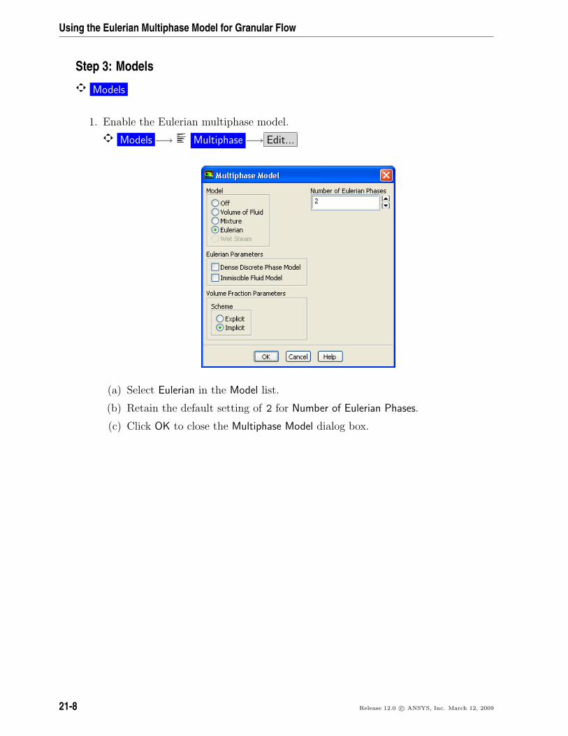
1. Enable the Eulerian multiphase model.

Models −→ Multiphase −→ Edit...

(a) Select Eulerian in the Model list.

(b) Retain the default setting of 2 for Number of Eulerian Phases.

(c) Click OK to close the Multiphase Model dialog box.



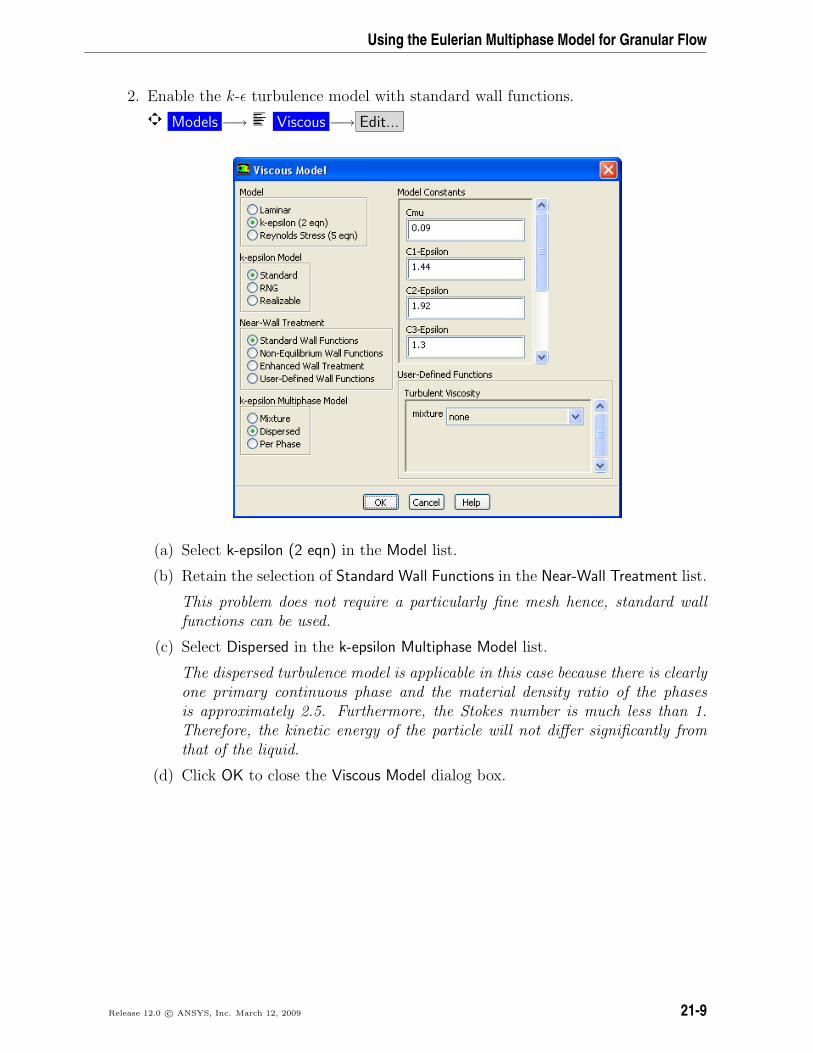
2. Enable the k-ε turbulence model with standard wall functions.

Models −→ Viscous −→ Edit...

(a) Select k-epsilon (2 eqn) in the Model list.

(b) Retain the selection of Standard Wall Functions in the Near-Wall Treatment list.

This problem does not require a particularly fine mesh hence, standard wallfunctions can be used.

(c) Select Dispersed in the k-epsilon Multiphase Model list.

The dispersed turbulence model is applicable in this case because there is clearlyone primary continuous phase and the material density ratio of the phasesis approximately 2.5. Furthermore, the Stokes number is much less than 1.Therefore, the kinetic energy of the particle will not differ significantly fromthat of the liquid.

(d) Click OK to close the Viscous Model dialog box.



Step 4: Materials

Materials

In this step, you will add liquid water to the list of fluid materials by copying it from theANSYS FLUENT materials database and create a new material called sand.

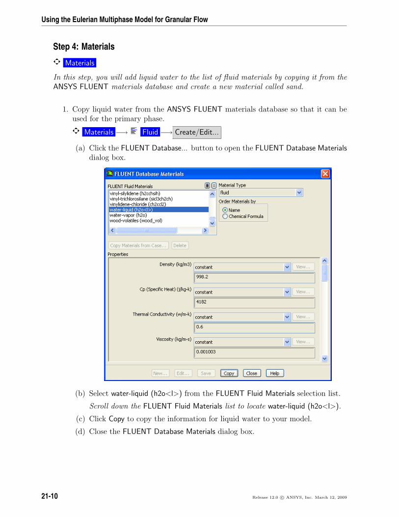
1. Copy liquid water from the ANSYS FLUENT materials database so that it can beused for the primary phase.

Materials −→ Fluid −→ Create/Edit...

(a) Click the FLUENT Database... button to open the FLUENT Database Materialsdialog box.

(b) Select water-liquid (h2o<l>) from the FLUENT Fluid Materials selection list.

Scroll down the FLUENT Fluid Materials list to locate water-liquid (h2o<l>).

(c) Click Copy to copy the information for liquid water to your model.

(d) Close the FLUENT Database Materials dialog box.



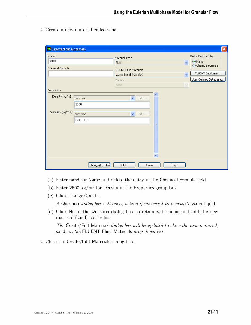
2. Create a new material called sand.

(a) Enter sand for Name and delete the entry in the Chemical Formula field.

(b) Enter 2500 kg/m3 for Density in the Properties group box.

(c) Click Change/Create.

A Question dialog box will open, asking if you want to overwrite water-liquid.

(d) Click No in the Question dialog box to retain water-liquid and add the newmaterial (sand) to the list.

The Create/Edit Materials dialog box will be updated to show the new material,sand, in the FLUENT Fluid Materials drop-down list.

3. Close the Create/Edit Materials dialog box.



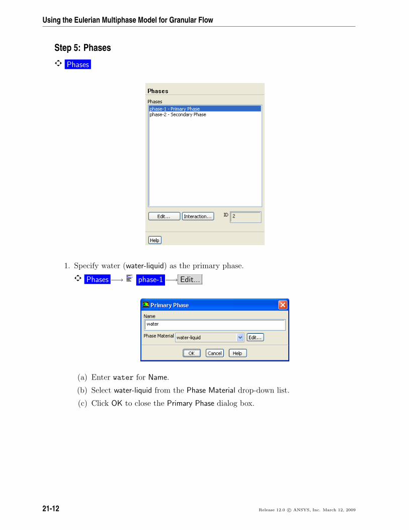
Step 5: Phases

Phases

1. Specify water (water-liquid) as the primary phase.

Phases −→ phase-1 −→ Edit...

(a) Enter water for Name.

(b) Select water-liquid from the Phase Material drop-down list.

(c) Click OK to close the Primary Phase dialog box.



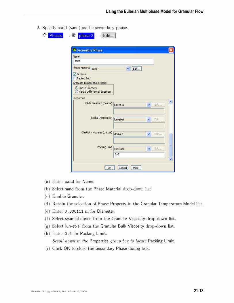
2. Specify sand (sand) as the secondary phase.

Phases −→ phase-2 −→ Edit...

(a) Enter sand for Name.

(b) Select sand from the Phase Material drop-down list.

(c) Enable Granular.

(d) Retain the selection of Phase Property in the Granular Temperature Model list.

(e) Enter 0.000111 m for Diameter.

(f) Select syamlal-obrien from the Granular Viscosity drop-down list.

(g) Select lun-et-al from the Granular Bulk Viscosity drop-down list.

(h) Enter 0.6 for Packing Limit.

Scroll down in the Properties group box to locate Packing Limit.

(i) Click OK to close the Secondary Phase dialog box.



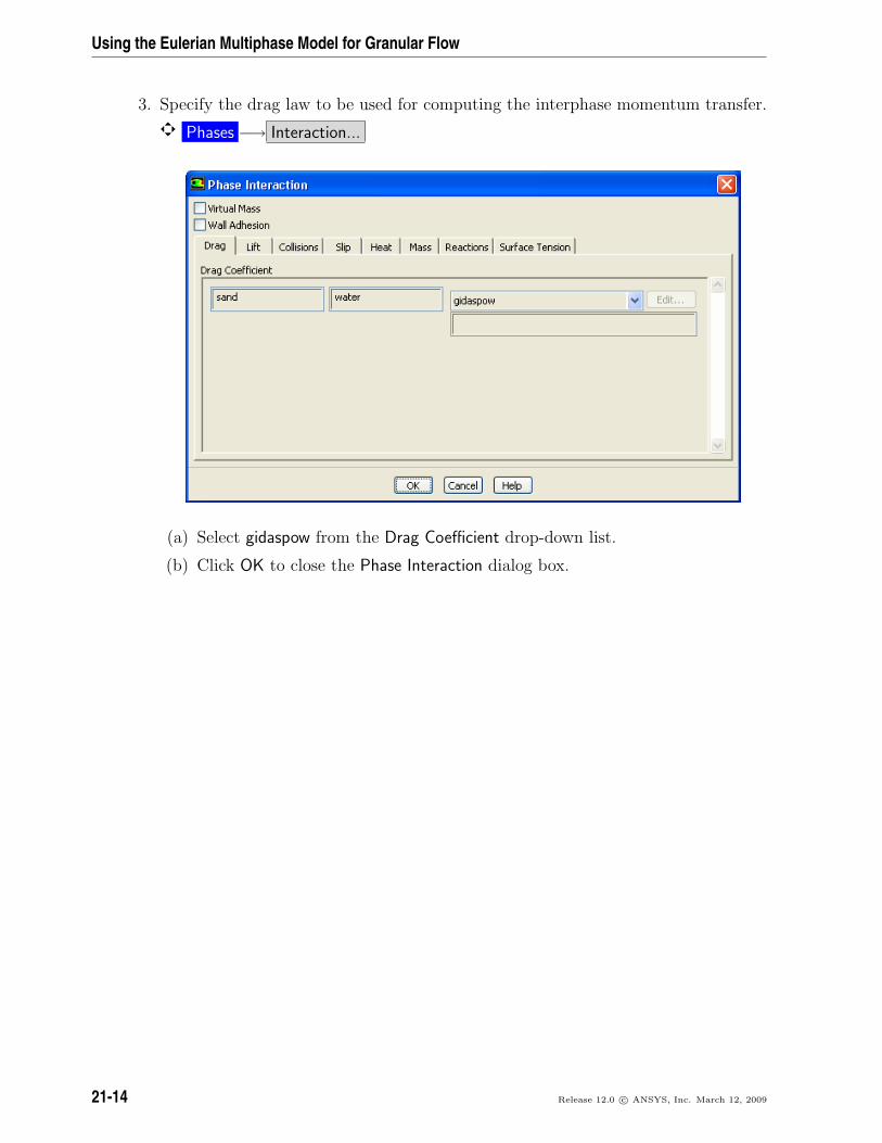
3. Specify the drag law to be used for computing the interphase momentum transfer.

Phases −→ Interaction...

(a) Select gidaspow from the Drag Coefficient drop-down list.

(b) Click OK to close the Phase Interaction dialog box.



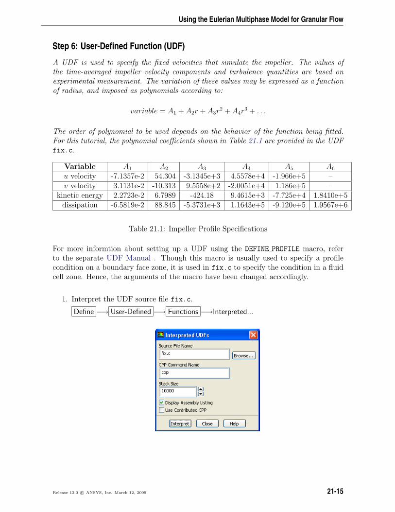
Step 6: User-Defined Function (UDF)

A UDF is used to specify the fixed velocities that simulate the impeller. The values ofthe time-averaged impeller velocity components and turbulence quantities are based onexperimental measurement. The variation of these values may be expressed as a functionof radius, and imposed as polynomials according to:

variable = A1 + A2r + A3r2 + A4r

3 + . . .

The order of polynomial to be used depends on the behavior of the function being fitted.For this tutorial, the polynomial coefficients shown in Table 21.1 are provided in the UDFfix.c.

Variable A1 A2 A3 A4 A5 A6

u velocity -7.1357e-2 54.304 -3.1345e+3 4.5578e+4 -1.966e+5 –v velocity 3.1131e-2 -10.313 9.5558e+2 -2.0051e+4 1.186e+5 –

kinetic energy 2.2723e-2 6.7989 -424.18 9.4615e+3 -7.725e+4 1.8410e+5dissipation -6.5819e-2 88.845 -5.3731e+3 1.1643e+5 -9.120e+5 1.9567e+6

Table 21.1: Impeller Profile Specifications

For more informtion about setting up a UDF using the DEFINE PROFILE macro, referto the separate UDF Manual . Though this macro is usually used to specify a profilecondition on a boundary face zone, it is used in fix.c to specify the condition in a fluidcell zone. Hence, the arguments of the macro have been changed accordingly.

1. Interpret the UDF source file fix.c.

Define −→ User-Defined −→ Functions −→Interpreted...



(a) Enter fix.c for Source File Name.

If the UDF source file is not in your working folder, you must enter the entirefolder path for Source File Name instead of just entering the file name. Alterna-tively, click Browse... and select fix.c in the eulerian multiphase granular

folder that was created after you unzipped the original file.

(b) Enable Display Assembly Listing.

The Display Assembly Listing option displays the assembly language code in theconsole as the function compiles.

(c) Click Interpret to interpret the UDF.

(d) Close the Interpreted UDFs dialog box.

Note: The name and contents of the UDF are stored in the case file whenyou save the case file.

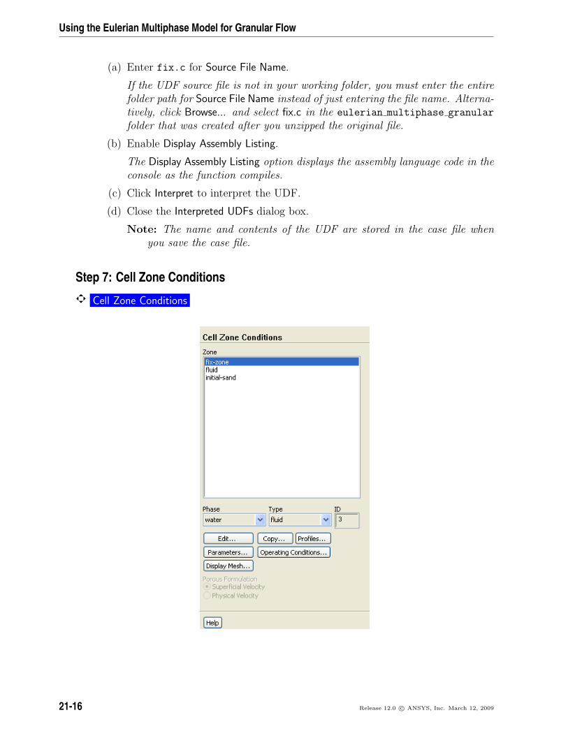
Step 7: Cell Zone Conditions

Cell Zone Conditions



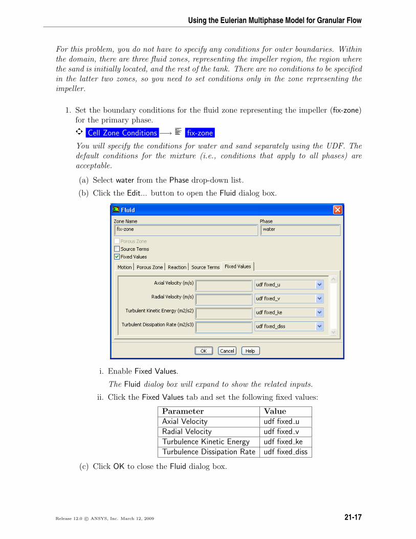
For this problem, you do not have to specify any conditions for outer boundaries. Withinthe domain, there are three fluid zones, representing the impeller region, the region wherethe sand is initially located, and the rest of the tank. There are no conditions to be specifiedin the latter two zones, so you need to set conditions only in the zone representing theimpeller.

1. Set the boundary conditions for the fluid zone representing the impeller (fix-zone)for the primary phase.

Cell Zone Conditions −→ fix-zone

You will specify the conditions for water and sand separately using the UDF. Thedefault conditions for the mixture (i.e., conditions that apply to all phases) areacceptable.

(a) Select water from the Phase drop-down list.

(b) Click the Edit... button to open the Fluid dialog box.

i. Enable Fixed Values.

The Fluid dialog box will expand to show the related inputs.

ii. Click the Fixed Values tab and set the following fixed values:

Parameter ValueAxial Velocity udf fixed uRadial Velocity udf fixed vTurbulence Kinetic Energy udf fixed keTurbulence Dissipation Rate udf fixed diss

(c) Click OK to close the Fluid dialog box.



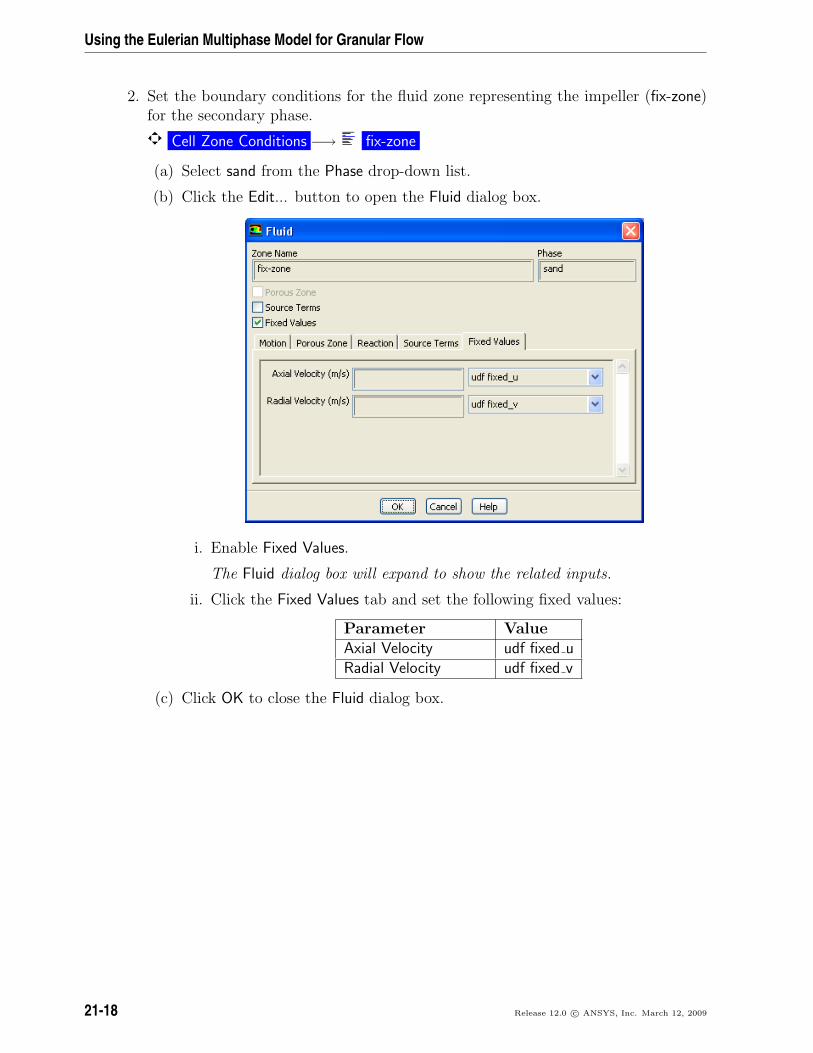
2. Set the boundary conditions for the fluid zone representing the impeller (fix-zone)for the secondary phase.

Cell Zone Conditions −→ fix-zone

(a) Select sand from the Phase drop-down list.

(b) Click the Edit... button to open the Fluid dialog box.

i. Enable Fixed Values.

The Fluid dialog box will expand to show the related inputs.

ii. Click the Fixed Values tab and set the following fixed values:

Parameter ValueAxial Velocity udf fixed uRadial Velocity udf fixed v

(c) Click OK to close the Fluid dialog box.



Step 8: Solution

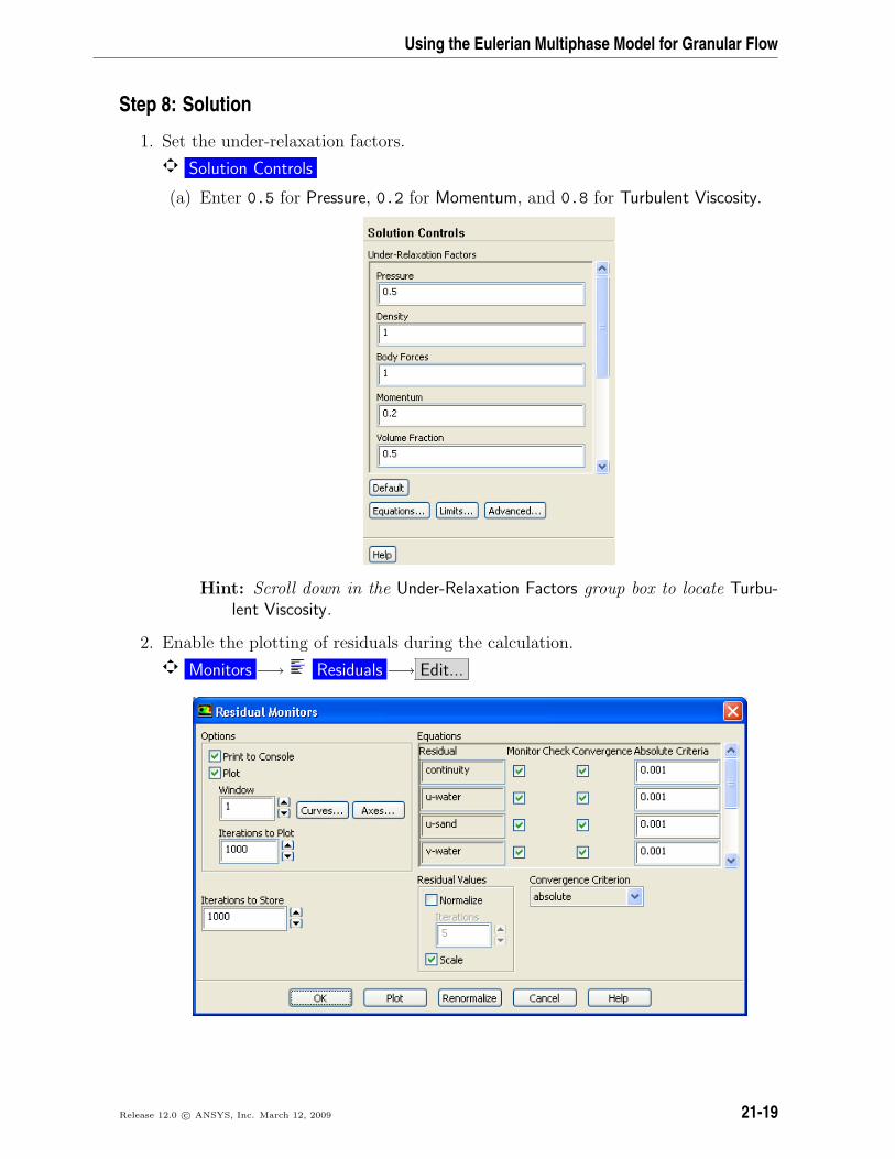
1. Set the under-relaxation factors.

Solution Controls

(a) Enter 0.5 for Pressure, 0.2 for Momentum, and 0.8 for Turbulent Viscosity.

Hint: Scroll down in the Under-Relaxation Factors group box to locate Turbu-lent Viscosity.

2. Enable the plotting of residuals during the calculation.

Monitors −→ Residuals −→ Edit...



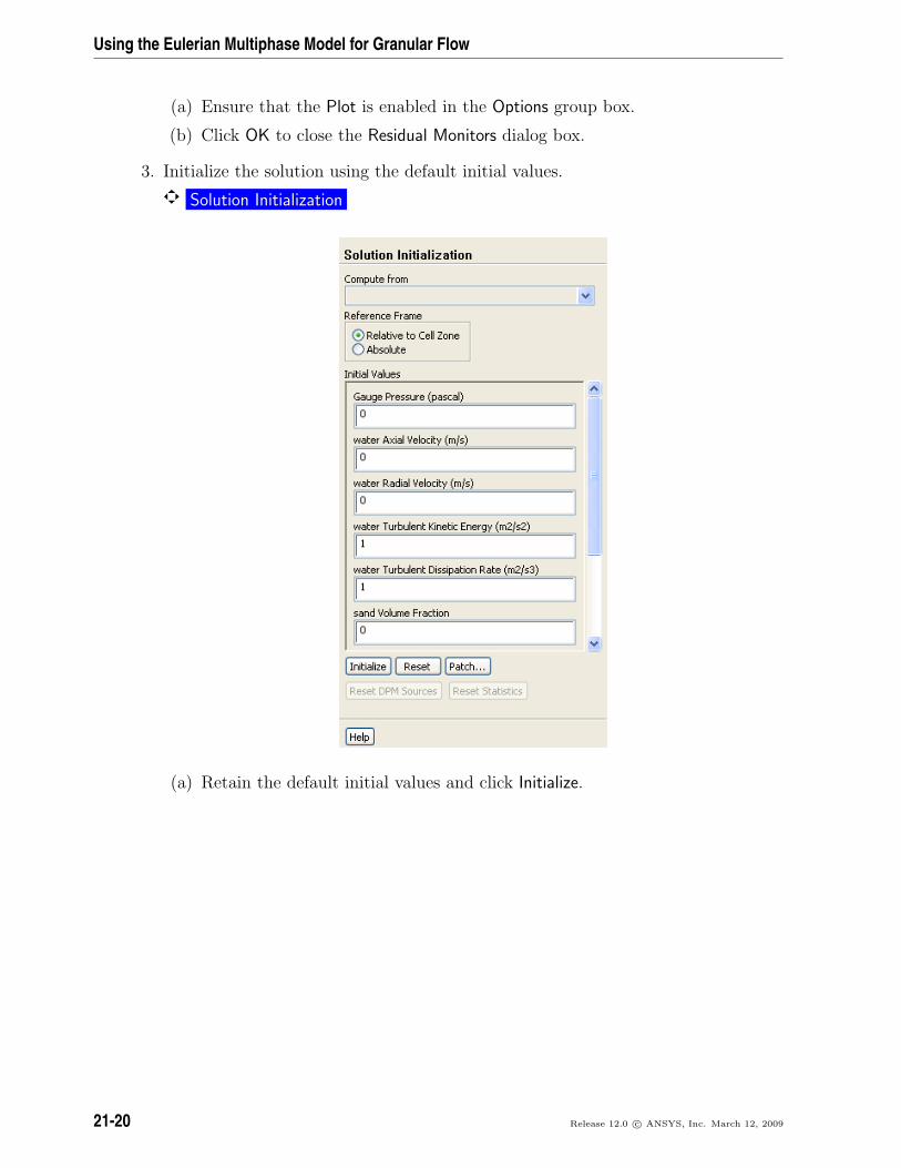
(a) Ensure that the Plot is enabled in the Options group box.

(b) Click OK to close the Residual Monitors dialog box.

3. Initialize the solution using the default initial values.

Solution Initialization

(a) Retain the default initial values and click Initialize.



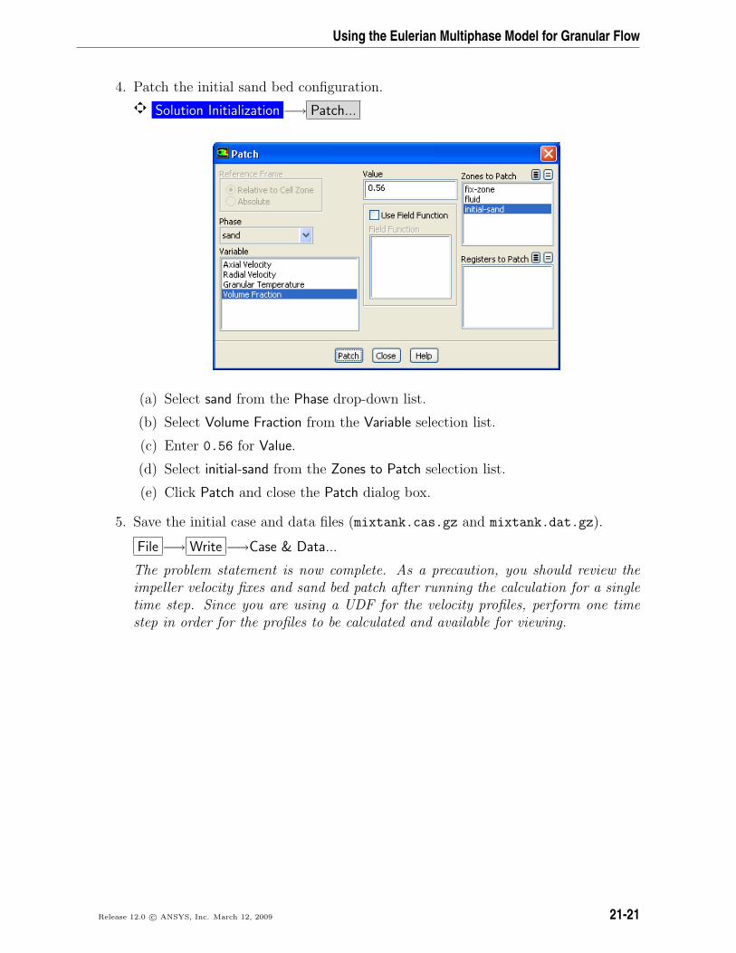
4. Patch the initial sand bed configuration.

Solution Initialization −→ Patch...

(a) Select sand from the Phase drop-down list.

(b) Select Volume Fraction from the Variable selection list.

(c) Enter 0.56 for Value.

(d) Select initial-sand from the Zones to Patch selection list.

(e) Click Patch and close the Patch dialog box.

5. Save the initial case and data files (mixtank.cas.gz and mixtank.dat.gz).

File −→ Write −→Case & Data...

The problem statement is now complete. As a precaution, you should review theimpeller velocity fixes and sand bed patch after running the calculation for a singletime step. Since you are using a UDF for the velocity profiles, perform one timestep in order for the profiles to be calculated and available for viewing.



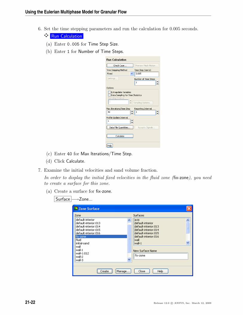
6. Set the time stepping parameters and run the calculation for 0.005 seconds.

Run Calculation

(a) Enter 0.005 for Time Step Size.

(b) Enter 1 for Number of Time Steps.

(c) Enter 40 for Max Iterations/Time Step.

(d) Click Calculate.

7. Examine the initial velocities and sand volume fraction.

In order to display the initial fixed velocities in the fluid zone (fix-zone), you needto create a surface for this zone.

(a) Create a surface for fix-zone.

Surface −→Zone...



i. Select fix-zone from the Zone selection list and click Create.

The default name is the same as the zone name. ANSYS FLUENT willautomatically assign the default name to the new surface when it is created.The new surface will be added to the Surfaces selection list in the ZoneSurface dialog box.

ii. Close the Zone Surface dialog box.

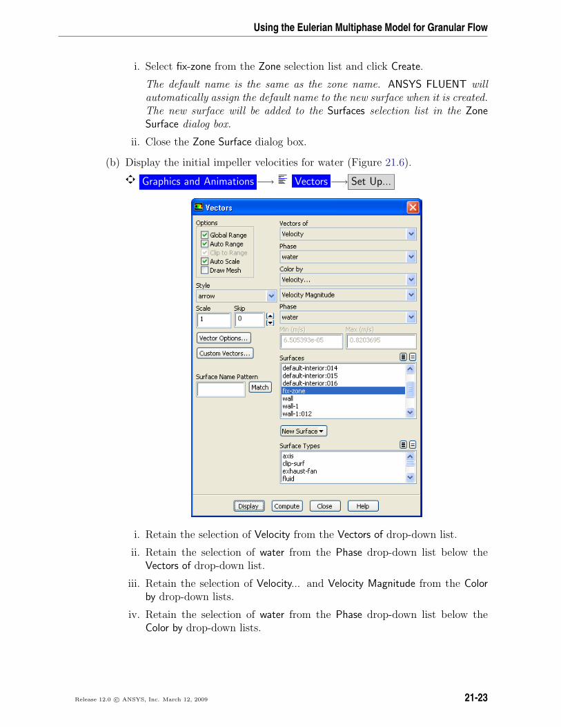
(b) Display the initial impeller velocities for water (Figure 21.6).

Graphics and Animations −→ Vectors −→ Set Up...

i. Retain the selection of Velocity from the Vectors of drop-down list.

ii. Retain the selection of water from the Phase drop-down list below theVectors of drop-down list.

iii. Retain the selection of Velocity... and Velocity Magnitude from the Colorby drop-down lists.

iv. Retain the selection of water from the Phase drop-down list below theColor by drop-down lists.



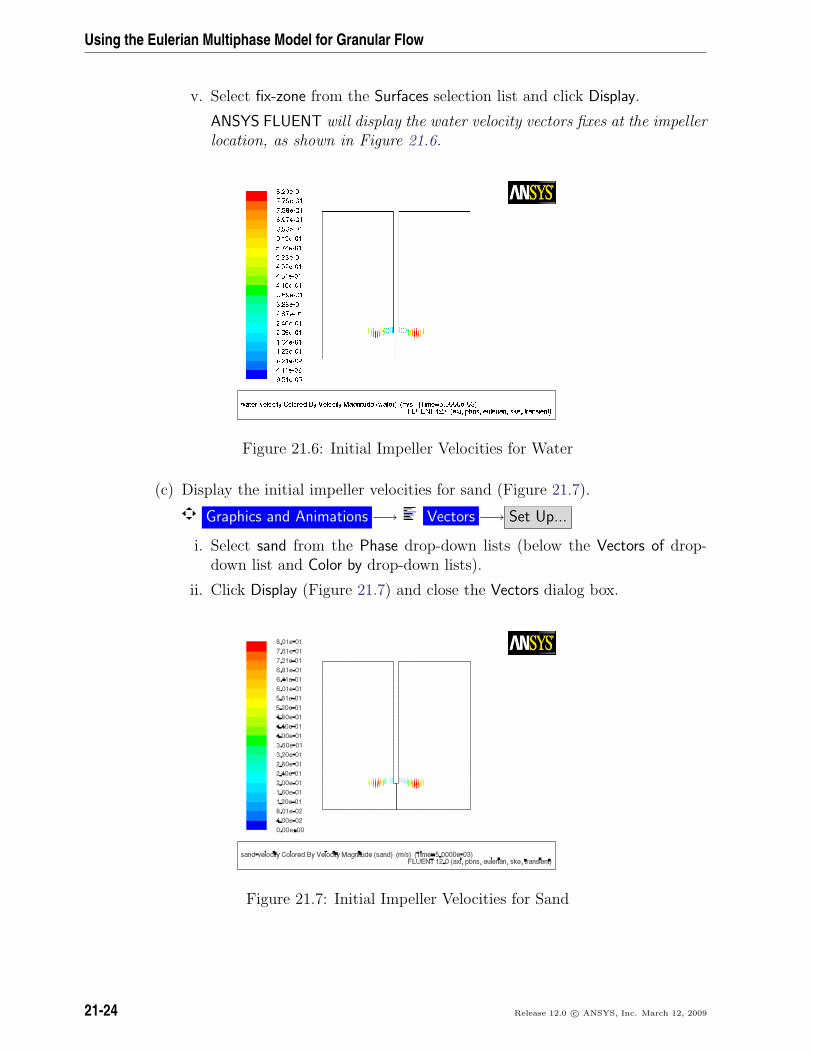
v. Select fix-zone from the Surfaces selection list and click Display.

ANSYS FLUENT will display the water velocity vectors fixes at the impellerlocation, as shown in Figure 21.6.

Figure 21.6: Initial Impeller Velocities for Water

(c) Display the initial impeller velocities for sand (Figure 21.7).


i. Select sand from the Phase drop-down lists (below the Vectors of drop-down list and Color by drop-down lists).

ii. Click Display (Figure 21.7) and close the Vectors dialog box.

Figure 21.7: Initial Impeller Velocities for Sand



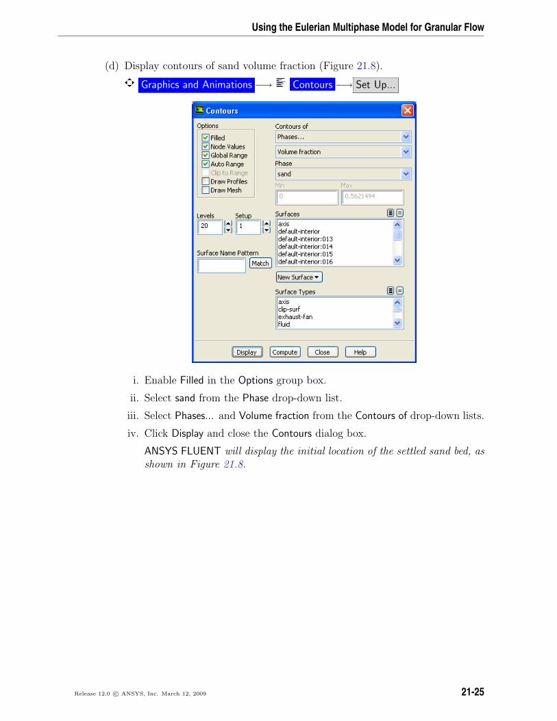
(d) Display contours of sand volume fraction (Figure 21.8).

Graphics and Animations −→ Contours −→ Set Up...

i. Enable Filled in the Options group box.

ii. Select sand from the Phase drop-down list.

iii. Select Phases... and Volume fraction from the Contours of drop-down lists.

iv. Click Display and close the Contours dialog box.

ANSYS FLUENT will display the initial location of the settled sand bed, asshown in Figure 21.8.



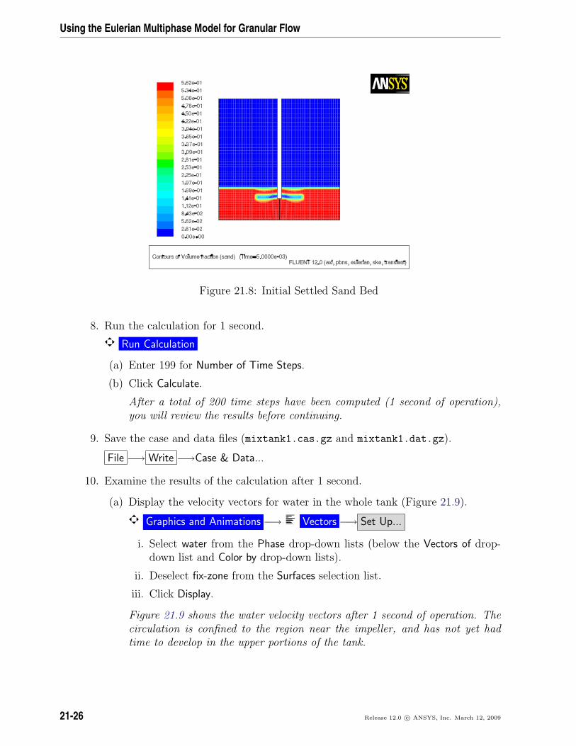
Figure 21.8: Initial Settled Sand Bed

8. Run the calculation for 1 second.

Run Calculation

(a) Enter 199 for Number of Time Steps.

(b) Click Calculate.

After a total of 200 time steps have been computed (1 second of operation),you will review the results before continuing.

9. Save the case and data files (mixtank1.cas.gz and mixtank1.dat.gz).


10. Examine the results of the calculation after 1 second.

(a) Display the velocity vectors for water in the whole tank (Figure 21.9).


i. Select water from the Phase drop-down lists (below the Vectors of drop-down list and Color by drop-down lists).

ii. Deselect fix-zone from the Surfaces selection list.

iii. Click Display.

Figure 21.9 shows the water velocity vectors after 1 second of operation. Thecirculation is confined to the region near the impeller, and has not yet hadtime to develop in the upper portions of the tank.



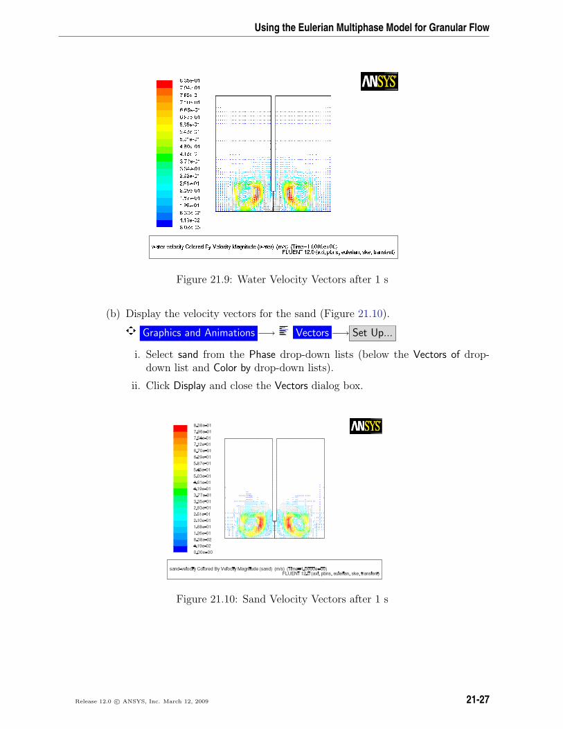
Figure 21.9: Water Velocity Vectors after 1 s

(b) Display the velocity vectors for the sand (Figure 21.10).


i. Select sand from the Phase drop-down lists (below the Vectors of drop-down list and Color by drop-down lists).

ii. Click Display and close the Vectors dialog box.

Figure 21.10: Sand Velocity Vectors after 1 s



Figure 21.10 shows the sand velocity vectors after 1 second of operation. Thecirculation of sand around the impeller is significant, but note that no sandvectors are plotted in the upper part of the tank, where the sand is not yetpresent.

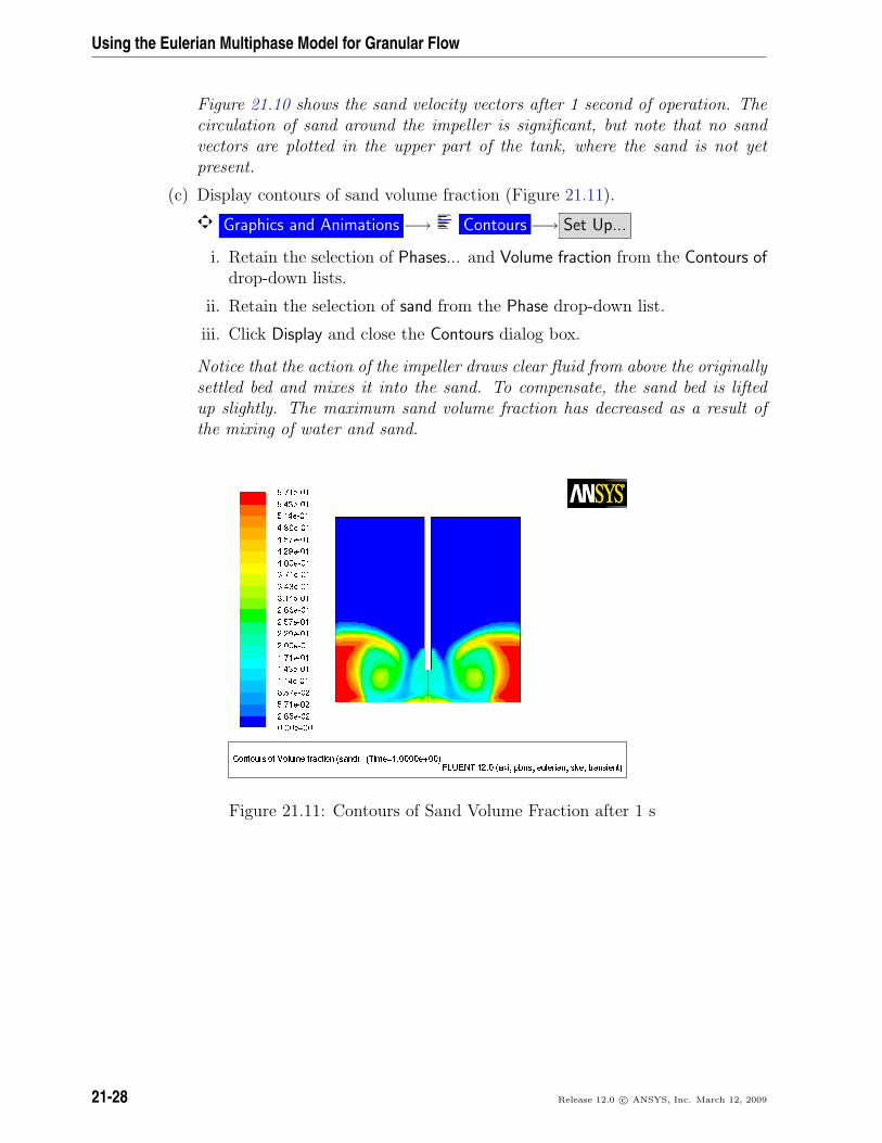
(c) Display contours of sand volume fraction (Figure 21.11).


i. Retain the selection of Phases... and Volume fraction from the Contours ofdrop-down lists.

ii. Retain the selection of sand from the Phase drop-down list.

iii. Click Display and close the Contours dialog box.

Notice that the action of the impeller draws clear fluid from above the originallysettled bed and mixes it into the sand. To compensate, the sand bed is liftedup slightly. The maximum sand volume fraction has decreased as a result ofthe mixing of water and sand.

Figure 21.11: Contours of Sand Volume Fraction after 1 s



11. Continue the calculation for another 19 seconds.

Run Calculation

(a) Set the Time Step Size to 0.01.

The initial calculation was performed with a very small time step size to sta-bilize the solution. After the initial calculation, you can increase the time stepto speed up the calculation.

(b) Enter 1900 for Number of Time Steps.

(c) Click Calculate.

The transient calculation will continue upto 20 seconds.

12. Save the case and data files (mixtank20.cas.gz and mixtank20.dat.gz).


Step 9: Postprocessing

You will now examine the progress of the sand and water in the mixing tank after a totalof 20 seconds. The mixing tank has nearly, but not quite, reached a steady flow solution.

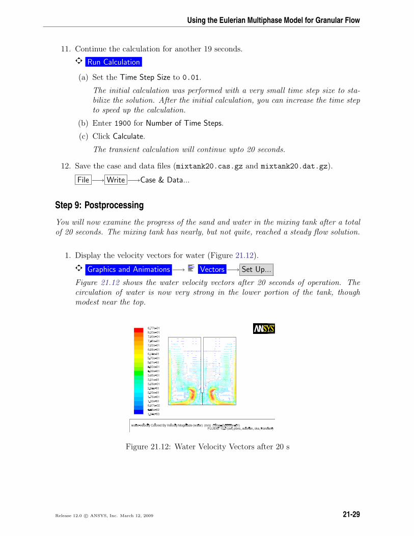
1. Display the velocity vectors for water (Figure 21.12).


Figure 21.12 shows the water velocity vectors after 20 seconds of operation. Thecirculation of water is now very strong in the lower portion of the tank, thoughmodest near the top.

Figure 21.12: Water Velocity Vectors after 20 s



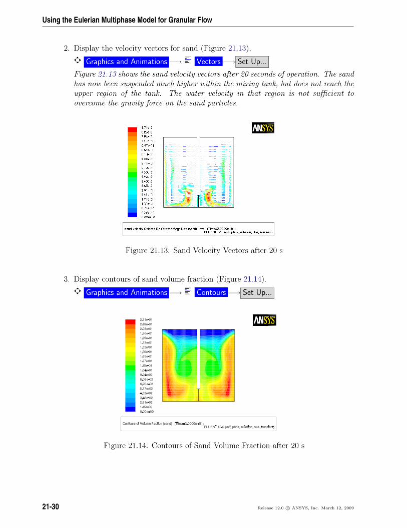
2. Display the velocity vectors for sand (Figure 21.13).


Figure 21.13 shows the sand velocity vectors after 20 seconds of operation. The sandhas now been suspended much higher within the mixing tank, but does not reach theupper region of the tank. The water velocity in that region is not sufficient toovercome the gravity force on the sand particles.

Figure 21.13: Sand Velocity Vectors after 20 s

3. Display contours of sand volume fraction (Figure 21.14).


Figure 21.14: Contours of Sand Volume Fraction after 20 s



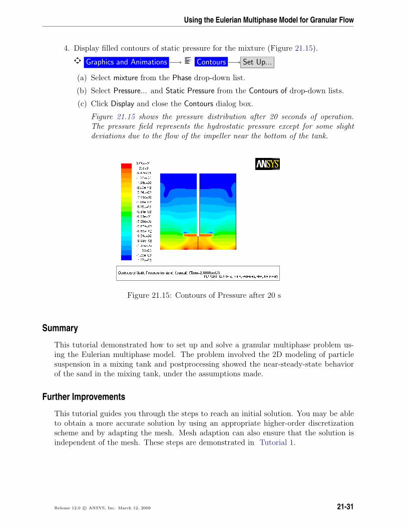
4. Display filled contours of static pressure for the mixture (Figure 21.15).


(a) Select mixture from the Phase drop-down list.

(b) Select Pressure... and Static Pressure from the Contours of drop-down lists.

(c) Click Display and close the Contours dialog box.

Figure 21.15 shows the pressure distribution after 20 seconds of operation.The pressure field represents the hydrostatic pressure except for some slightdeviations due to the flow of the impeller near the bottom of the tank.

Figure 21.15: Contours of Pressure after 20 s

Summary

This tutorial demonstrated how to set up and solve a granular multiphase problem us-ing the Eulerian multiphase model. The problem involved the 2D modeling of particlesuspension in a mixing tank and postprocessing showed the near-steady-state behaviorof the sand in the mixing tank, under the assumptions made.

Further Improvements

This tutorial guides you through the steps to reach an initial solution. You may be ableto obtain a more accurate solution by using an appropriate higher-order discretizationscheme and by adapting the mesh. Mesh adaption can also ensure that the solution isindependent of the mesh. These steps are demonstrated in Tutorial 1.




Documents

Tutorial 21. Using the Eulerian Multiphase Model for Granular …barbertj/CFD Training/Fluent 12/t… · · 2009-10-07Using the Eulerian Multiphase Model for ... Use FLUENT Launcher