© Fluent Inc. 9/14/20151 Fluent Software Training TRN-98-006 Modeling Multiphase Flows

© Fluent Inc. 04/19/231

Fluent Software TrainingTRN-98-006

Modeling Multiphase Flows

© Fluent Inc. 04/19/232


Outline

Definitions; Examples of flow regimes Description of multiphase models in FLUENT 5 and FLUENT 4.5 How to choose the correct model for your application Summary and guidelines

© Fluent Inc. 04/19/233


Definitions Multiphase flow is simultaneous flow of

Matters with different phases( i.e. gas, liquid or solid). Matters with different chemical substances but with the same phase (i.e.

liquid-liquid like oil-water).

Primary and secondary phases One of the phases is considered continuous (primary) and others (secondary)

are considered to be dispersed within the continuous phase. A diameter has to be assigned for each secondary phase to calculate its

interaction (drag) with the primary phase (except for VOF model). Dilute phase vs. Dense phase;

Refers to the volume fraction of secondary phase(s)

Volume fraction of a phase = Volume of the phase in a cell/domainVolume of the cell/domain

© Fluent Inc. 04/19/234


Flow Regimes

Multiphase flow can be classified by the following regimes:

Bubbly flow: Discrete gaseous or fluid bubbles in a continuous fluid

Droplet flow: Discrete fluid droplets in a continuous gas

Particle-laden flow: Discrete solid particles in a continuous fluid

Slug flow: Large bubbles (nearly filling cross-section) in a continuous fluid

Annular flow: Continuous fluid along walls, gas in center

Stratified/free-surface flow: Immiscible fluids separated by a clearly-defined interface

bubbly flow droplet flow

particle-laden flow

slug flow

annular flow free-surface flow

© Fluent Inc. 04/19/235


Flow Regimes

User must know a priori what the flow field looks like: Flow regime,

bubbly flow , slug flow, etc. Model one flow regime at a time.

– Multiple flow regime can be predicted if they are predicted by one model e.g. slug flow and annular flow may coexist since both are predicted by VOF model.

turbulent or laminar, dilute or dense, bubble or particle diameter (mainly for drag considerations).

© Fluent Inc. 04/19/236


Multiphase Models

Four models for multiphase flows currently available in structured FLUENT 4.5

Lagrangian dispersed phase model (DPM) Eulerian Eulerian model Eulerian Granular model Volume of fluid (VOF) model

Unstructured FLUENT 5 Lagrangian dispersed phase model (DPM) Volume of fluid model (VOF) Algebraic Slip Mixture Model (ASMM) Cavitation Model

© Fluent Inc. 04/19/237


Dispersed Phase Model

© Fluent Inc. 04/19/238


Dispersed Phase Model Appropriate for modeling particles, droplets, or bubbles

dispersed (at low volume fraction; less than 10%) in continuous fluid phase:

Spray dryers Coal and liquid fuel combustion Some particle-laden flows

Computes trajectories of particle (or droplet or bubble) streams in continuous phase.

Computes heat, mass, and momentum transfer between dispersed and continuous phases.

Neglects particle-particle interaction. Particles loading can be as high as fluid loading Computes steady and unsteady (FLUENT 5) particle tracks.

Particle trajectories in a spray dryer

© Fluent Inc. 04/19/239


Particle trajectories computed by solving equations of motion of the particle in Lagrangian reference frame:

where represents additional forces due to: virtual mass and pressure gradients rotating reference frames temperature gradients Brownian motion (FLUENT 5) Saffman lift (FLUENT 5) user defined

Particle Trajectory Calculations

ppppp Fguuf

dt

ud //)()(drag

F

© Fluent Inc. 04/19/2310


Coupling Between Phases One-Way Coupling

Fluid phase influences particulate phase via drag and turbulence transfer. Particulate phase have no influence on the gas phase.

Two-Way Coupling Fluid phase influences particulate phase via drag and turbulence transfer. Particulate phase influences fluid phase via source terms of mass,

momentum, and energy. Examples include:

Inert particle heating and cooling Droplet evaporation Droplet boiling Devolatilization Surface combustion

© Fluent Inc. 04/19/2311


To determine impact of dispersed phase on continuous phase flow field, coupled calculation procedure is used:

Procedure is repeated until both flow fields are unchanged.

DPM: Calculation Procedure

continuous phase flow field calculation

particle trajectory calculation

interphase heat, mass, and momentum exchange

© Fluent Inc. 04/19/2312


Turbulent Dispersion of Particles

Dispersion of particle due to turbulent fluctuations in the flow can be modeled using either:

Discrete Random Walk Tracking (stochastic approach)

Particle Cloud Tracking

© Fluent Inc. 04/19/2313


User Defined Function Access in DPM

User defined functions (UDF’s) are provided for access to the discrete phase model. Functions are provided for user defined:

drag external force laws for reacting particles and droplets customized switching between laws output for sample planes erosion/accretion rates access to particle definition at injection time scalars associated with each particle and access at each particle time step

(possible to integrate scalar variables over life of particle)

FLUENT 5

© Fluent Inc. 04/19/2314


Eulerian-Eulerian Multiphase ModelFLUENT 4.5

10s 70s 120s

waterwater

airair

Becker et al. 1992

Locally Aerated Bubble Column

© Fluent Inc. 04/19/2315


Eulerian Multiphase Model

Appropriate for modeling gas-liquid or liquid-liquid flows (droplets or bubbles of secondary phase(s) dispersed in continuous fluid phase (primary phase)) where:

Phases mix or separate Bubble/droplet volume fractions from 0 to

100% Evaporation Boiling Separators Aeration

Inappropriate for modeling stratified or free-surface flows.

Volume fraction of water

Stream functioncontours for water

Boiling water in a container

© Fluent Inc. 04/19/2316



Solves momentum, enthalpy, continuity, and species equations for each phase and tracks volume fractions.

Uses a single pressure field for all phases. Interaction between mean flow field of

phases is expressed in terms of a drag, virtual and lift forces.

Several formulations for drag is provided. Alternative drag laws can be formulated

via UDS. Other forces can be applied through UDS. Gas sparger in a mixing tank:

contours of volume fraction with velocity vectors

© Fluent Inc. 04/19/2317



Can solve for multiple species and homogeneous reactions in each phase.

Heterogeneous reactions can be done through UDS.

Allows for heat and mass transfer between phases.

Turbulence models for dilute and dense phase regimes.

© Fluent Inc. 04/19/2318


Mass Transfer

Evaporation/Condensation. For liquid temperatures saturation temperature, evaporation rate:

For vapor temperatures saturation temperature, condensation rate:

User specifies saturation temperature and, if desired, “time relaxation parameters” rl and rv . (Wen Ho Lee (1979))

Unidirectional mass transfer, is constant

User Defined Subroutine for mass transfer

sat

satlllvv T

TTrm

sat

vsatvvll T

TTrm

1212 rm

r

© Fluent Inc. 04/19/2319


Eulerian Multiphase Model: Turbulence Time averaging is needed to obtain smoothed quantities from the

space averaged instantaneous equations. Two methods available for modeling turbulence in multiphase flows

within context of standard k-model: Dispersed turbulence model (default) appropriate when both of these

conditions are met: Number of phases is limited to two:

Continuous (primary) phase Dispersed (secondary) phase

Secondary phase must be dilute. Secondary turbulence model appropriate for turbulent multiphase flows

involving more than two phases or a non-dilute secondary phase. Choice of model depends on importance of secondary-phase

turbulence in your application.

© Fluent Inc. 04/19/2320


Eulerian Granular Multiphase Model: FLUENT 4.5

Volume fraction of air2D fluidized bed with a central jet

© Fluent Inc. 04/19/2321


Eulerian Granular Multiphase Model: Extension of Eulerian-Eulerian model for flow of granular

particles (secondary phases) in a fluid (primary)phase Appropriate for modeling:

Fluidized beds Risers Pneumatic lines Hoppers, standpipes Particle-laden flows in which:

Phases mix or separate Granular volume fractions can vary from 0 to packing limit

Circulating fluidized bed, Tsuo and Gidaspow (1990).

Solid velocity profiles Contours of solid volume fraction

© Fluent Inc. 04/19/2322


Eulerian Granular Multiphase Model: Overview

The fluid phase must be assigned as the primary phase. Multiple solid phase can be used to represent size distribution. Can calculate granular temperature (solids fluctuating energy) for each

solid phase. Calculates a solids pressure field for each solid phase.

All phases share fluid pressure field. Solids pressure controls the solids packing limit

Solids pressure, granular temperature conductivity, shear and bulk viscosity can be derived based on several kinetic theory formulations.

Gidaspow -good for dense fluidized bed applications Syamlal -good for a wide range of applications Sinclair -good for dilute and dense pneumatic

transport lines and risers

© Fluent Inc. 04/19/2323


Eulerian Granular Multiphase Model Frictional viscosity pushes the limit into the plastic regime.

Hoppers, standpipes Several choice of drag laws:

Drag laws can be modified using UDS. Heat transfer between phases is the same as in Eulerian/Eulerian multiphase model. Only unidirectional mass transfer model is available.

Rate of mass transfer can be modified using UDS. Homogeneous reaction can be modeled.

Heterogeneous reaction can be modeled using UDS. Can solve for enthalpy and multiple species for each phase. Physically based models for solid momentum and granular temperature boundary

conditions at the wall. Turbulence treatment is the same as in Eulerian-Eulerian model

Sinclair model provides additional turbulence model for solid phase

© Fluent Inc. 04/19/2324


Algebraic Slip Mixture ModelFLUENT 5

Courtesy of Fuller Company

© Fluent Inc. 04/19/2325


Algebraic Slip Mixture Model

Can substitute for Eulerian/Eulerian, Eulerian/Granular and Dispersed phase models Efficiently for Two phase flow problems:

Fluid/fluid separation or mixing: Sedimentation of uniform size particles in liquid. Flow of single size particles in a Cyclone.

Applicable to relatively small particles (<50 microns) and low volume fraction (<10%) when primary phase density is much smaller than the secondary phase density.

Air-water separation in a Tee junctionWater volume fraction

If possible, always choose the fluid with higher density as the primary phase.

© Fluent Inc. 04/19/2326


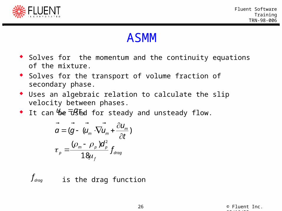
Solves for the momentum and the continuity equations of the mixture. Solves for the transport of volume fraction of secondary phase. Uses an algebraic relation to calculate the slip velocity between

phases. It can be used for steady and unsteady flow.

is the drag function

ASMM

prel au

))((t

uuuga m

mm

drag

f

ppm

p fd

18

)( 2

dragf

© Fluent Inc. 04/19/2327


Oil-Water Separation

Fluent 5 Results with ASMM Fluent v4.5 Eulerian Multiphase

Courtesy ofArco Exploration & Production TechnologyDr. Martin de Tezanos Pinto

© Fluent Inc. 04/19/2328


Cavitation Model ( Fluent 5) Predicts cavitation inception and approximate extension of cavity bubble. Solves for the momentum equation of the mixture Solves for the continuity equation of the mixture Assumes no slip velocity between the phases Solves for the transport of volume fraction of vapor phase.

Approximates the growth of the cavitation bubble using Rayleigh equation

Needs improvement: ability to predict collapse of cavity bubbles

Needs to solve for enthalpy equation and thermodynamic properties Solve for change of bubble size

l

v pp

dt

dR

3

)(2

l

vvv pp

Rm

3

)(23

© Fluent Inc. 04/19/2329


Cavitation model

© Fluent Inc. 04/19/2330


VOF Model

© Fluent Inc. 04/19/2331


Volume of Fluid Model Appropriate for flow where Immiscible

fluids have a clearly defined interface. Shape of the interface is of interest

Typical problems: Jet breakup Motion of large bubbles in a liquid Motion of liquid after a dam break

(shown at right) Steady or transient tracking of any

liquid-gas interface Inappropriate for:

Flows involving small (compared to a control volume) bubbles

Bubble columns

© Fluent Inc. 04/19/2332


Volume Fraction Assumes that each control volume contains just one phase (or the

interface between phases). For volume fraction of kth fluid, three conditions are possible:

k = 0 if cell is empty (of the kth fluid)

k = 1 if cell is full (of the kth fluid)

0 < k < 1 if cell contains the interface between the fluids

Tracking of interface(s) between phases is accomplished by solution of a volume fraction continuity equation for each phase:

Mass transfer between phases can be modeled by using a user-defined subroutine to specify a nonzero value for Sk

.

Multiple interfaces can be simulated Can not resolve details of the interface smaller than the mesh size

kj

k

ikt

ux

S

© Fluent Inc. 04/19/2333


VOF

Solves one set of momentum equations for all fluids.

Surface tension and wall adhesion modeled with an additional source term in momentum eqn.

For turbulent flows, single set of turbulence transport equations solved.

Solves for species conservation equations for primary phase .

jji

j

j

i

ijji

ij Fg

x

u

x

u

xx

Puu

xu

t

)()()(

© Fluent Inc. 04/19/2334


Formulations of VOF Model Time-dependent with a explicit schemes:

geometric linear slope reconstruction (default in FLUENT 5) Donor-acceptor (default in FLUENT 4.5)

Best scheme for highly skewed hex mesh. Euler explicit

Use for highly skewed hex cells in hybrid meshes if default scheme fails. Use higher order discretization scheme for more accuracy.

Example: jet breakup

Time-dependent with implicit scheme: Used to compute steady-state solution when intermediate solution is not important.

More accurate with higher discretization scheme. Final steady-state solution is dependent on initial flow conditions There is not a distinct inflow boundary for each phase

Example: shape of liquid interface in centrifuge

Steady-state with implicit scheme: Used to compute steady-state solution using steady-state method.

More accurate with higher order discretization scheme. Must have distinct inflow boundary for each phase

Example: flow around ship’s hull

DecreasingAccuracy

© Fluent Inc. 04/19/2335


Comparison of Different Front Tracking Algorithms

2nd order upwind Donor - Acceptor

Geometric reconstruction Geometric reconstruction with tri mesh

© Fluent Inc. 04/19/2336


Surface Tension

Cylinder of water (5 x 1 cm) is surrounded by air in no gravity Surface is initially perturbed so that the diameter is 5% larger on ends The disturbance at the surface grows because of surface tension

© Fluent Inc. 04/19/2337


Wall Adhesion Wall adhesion is modeled by specification of contact angle that fluid

makes with wall. Large contact angle (> 90°) is applied to water at bottom of container in

zero-gravity field. An obtuse angle, as measured in water, will form at walls. As water tries to satisfy contact angle condition, it detaches from bottom

and moves slowly upward, forming a bubble.

© Fluent Inc. 04/19/2338


Choosing a Multiphase Model: Fluid-Fluid Flows (1)

Bubbly flow examples: Absorbers Evaporators Scrubbers Air lift pumps

Droplet flow examples: Atomizers Gas cooling Dryers

Slug flow examples: Large bubble motion in pipes or tanks

Separated flows free surface, annular flows, stratified flows, liquid films

CavitationFlotationAerationNuclear reactors

Combustors Scrubbers Cryogenic pumping

© Fluent Inc. 04/19/2339


Choosing a Multiphase Model: Gas-Liquid Flows (2)

Volume fraction Model CommentsLess than 10% DPM

Cavitation

Ignores bubble coalescence or particle-particle interaction.

Inception of cavitation and its approximate extension.

All Values ASMM

Eulerian

Applies to two phase flows only. If density ofprimary phase is much less than the density of thesecondary phase, restricts to applications with smalldiameter and low volume fraction of the Secondayphase.

For large bubbles either use Vof or modify the Draglaw. Ignores bubble coalescence or interaction.

All Values VOF Bubbles should span across several cells.Applicableto separated flows: free surface flows, annular flows,liquid films, stratified flows.

© Fluent Inc. 04/19/2340


Choosing a Multiphase Model: Particle-Laden Flow

Examples: Cyclones Slurry transport Flotation Circulating bed reactors

Dust collectors Sedimentation Suspension Fluidized bed reactors

Volume fraction Model CommentsLess than 10% DPM

ASMM

Ignores bubble coalescence or particle-particleinteraction

Only one solid size. More efficient than DPM. Forliquid-solid applications can be used for highervolume fraction of solids but well below packinglimit.

All values EulerianGranular

Solve in a transient manner..

© Fluent Inc. 04/19/2341


Solution Guidelines

All multiphase calculations: Start with a single-phase calculation to establish broad flow patterns.

Eulerian multiphase calculations: Use COPY-PHASE-VELOCITIES to copy primary phase velocities to

secondary phases. Patch secondary volume fraction(s) as an initial condition. For a single outflow, use OUTLET rather than PRESSURE-INLET; for

multiple outflow boundaries, must use PRESSURE-INLET for each. For circulating fluidized beds, avoid symmetry planes. (They promote

unphysical cluster formation.) Set the “false time step for underrelaxation” to 0.001 Set normalizing density equal to physical density Compute a transient solution

© Fluent Inc. 04/19/2342


Solution Strategies (VOF) For explicit formulations for best and quick results:

use geometric reconstruction or donor-acceptor use PISO algorithm with under-relaxation factors up to 1.0

reduce time step if convergence problem arises. To ensure continuity, reduce termination criteria to 0.001 for pressure in multi-grid

solver solve VOF once per time-step

For implicit formulations: always use QUICK or second order upwind difference scheme for VOF equation. may increase VOF UNDER-RELAXATION from 0.2 (default ) to 0.5.

Use proper reference density to prevent round off errors. Use proper pressure interpolation scheme for hydrostatic consideration:

Body force weighted scheme for all types of cells PRESTO (only for quads and hexes)

© Fluent Inc. 04/19/2343


Summary Modeling multiphase flows is very complex, due to interdependence of

many variables. Accuracy of results directly related to appropriateness of model you

choose: For most applications with low volume fraction of particles, droplets, or

bubbles, use ASMM or DPM model . For particle-laden flows, Eulerian granular multiphase model is best. For separated gas-liquid flows (stratified, free-surface, etc.) VOF model is

best. For general, complex gas-liquid flows involving multiple flow regimes:

Select aspect of flow that is of most interest. Choose model that is most appropriate. Accuracy of results will not be as good as for others, since selected physical

model will be valid only for some flow regimes.

© Fluent Inc. 04/19/2344


Conservation equations Conservation of mass

Conservation of momentum

Conservation of enthalpy

qqqqqqqqqqqqq FPuuut

)(

n

ppqqqqqq mu

t 1

)(1

pqpq

n

ppq umR

qqqk

q

qqqqqqqq squdt

dphuh

t

.:)()(

)(1

pqpq

n

ppq hmQ

© Fluent Inc. 04/19/2345


Constitutive Equations

Frictional Flow Particles are in enduring contact and momentum transfer is through

friction Stresses from soil mechanics, Schaeffer (1987)

Description of frictional viscosity

is the second invariant of the deviatoric stress tensor

frictskinscollss ,,, ,max

)0( su

2

, 2

sin

I

Psfricts

2I

© Fluent Inc. 04/19/2346


Interphase Forces (cont.) Virtual Mass Effect: caused by relative acceleration between phases Drew

and Lahey (1990).

Virtual mass effect is significant when the second phase density is much smaller than the primary phase density (i.e., bubble column)

Lift Force: Caused by the shearing effect of the fluid onto the particle Drew and Lahey (1990).

Lift force usually insignificant compared to drag force except when the phases separate quickly and near boundaries

)()(, sss

ff

f

fsvmfsvm uut

uuu

t

uCK

)()(, fsffsLfsk uuuCK

© Fluent Inc. 04/19/2347


Eulerian Multiphase Model: Turbulence The transport equations for the model are of the form

Value of the parameters

k

kkkkkkk

k

tk

kkkkkkkkk

Gkkukt

)(

kkkkk

k

kk

tk

kkkkkkkkk

cGck

ut

}{)( 21

3.192.144.13.1109.0321 cccc k

© Fluent Inc. 04/19/2348


Comparison of Drag Laws

Fluid-solid drag functions

0

2

4

6

8

10

12

14

0.01 0.06 0.12 0.17 0.23 0.28 0.34 0.39 0.45 0.5 0.56

Solids volume fraction

f

Syamlal-O'Brien

Schuh et al.

Gidaspow A

Gidaspow B

Wen and Yu

Di Felice

Fluid-solid drag functions

0

50

100

150

200

250

300

0.01 0.07 0.13 0.19 0.25 0.31 0.37 0.43 0.49 0.55

Solids volume fraction

f

Syamlal-O'Brien

Schuh et al.

Gidaspow A

Gidaspow B

Wen and Yu

Di Felice

Relative Reynolds number 1 and 1000Particle diameter 0.001 mm

Arastoopour

Arastoopour

© Fluent Inc. 04/19/2349


Drag Force Models

Fluid-fluid drag functions

0

0.5

1

1.5

2

2.5

3

3.5

4

4.5

10 2460 4910 7360 9810 12260 14710

Re

CdSchiller and Naumann

Schuh et al.

Morsi et Alexander

1000Re44.0

1000ReRe15.0124 687.0

DC

2500Re4008.0

2500Re200Re/Re0135.0Re914.024

200Re0Re15.0124282.0

687.0

DC

(Re)are,,whereReRe 3212

321 faaa

aaaCD

Schiller and Naumann

Schuh et al.

Morsi and Alexander

© Fluent Inc. 04/19/2350


Solution Algorithms for Multiphase Flows

Coupled solver algorithms (more coupling between phases) Faster turn around and more stable numerics

High order discretization schemes for all phases. More accurate results

Implicit/Full EliminationAlgorithm v4.5

Implicit/Full EliminationAlgorithm v4.5

TDMA CoupledAlgorithm v4.5

TDMA CoupledAlgorithm v4.5

Multiphase Flow SolutionAlgorithms

Multiphase Flow SolutionAlgorithms

Only Eulerian/Eulerian model

© Fluent Inc. 04/19/2351


Heterogeneous Reactions in FLUENT4.5

Problem Description Two liquid e.g. (L1,L2) react and make solids e.g. (s1,s2) Reactions happen within liquid e.g. (L1-->L2) Reactions happen within solid e.g. (s1--->s2)

Solution! Consider a two phase liquid (primary) and solid (secondary)

liquid has two species L1, L2 solid has two species s1,s2

Reactions within each phase i.e. (L1-->L2) and (s1-->s2) can be set up as usual through GUI (like in single phase)

For heterogeneous reaction e.g. (L1+0.5L2-->0.2s1+s2)

© Fluent Inc. 04/19/2352


Heterogeneous Reactions in FLUENT 4.5

In usrmst.F calculate the net mass transfer between phases as a result of reactions

– Reactions could be two ways Assign this value to suterm

– If the net mass transfer is from primary to secondary the value should be negative and vica versa.

The time step and mass transfer rate should be such that the net volume fraction change would not be more than 5-10%.

In urstrm.F Adjust the mass fraction of each species by assigning a source or sink

value (+/-) according to mass transfer calculated above. Adjust the enthalp of each phase by the net amount of heat of reactions

and enthalpy transfer due to mass transfer. Again this will be in a form of a source term.

© Fluent Inc. 04/19/2353


Heterogeneous Reactions in FLUENT 4.5

Compile your version of the code Run Fluent and set up the case :

Enable time dependent, multiphase, temperature and species calculations. Define phases Enable mass transfer and multi-component multi-species option. Define species, homogeneous reactions within each phases Define properties Enable user defined mass transfer

GOOD LUCK!!

© Fluent Inc. 04/19/2354


Particle size

Descriptive terms Size range Example

Coarse solid 5 - 100 mm coal

Granular solid 0.3 - 5 mm sugar

Coarse powder 100-300 m salt, sand

Fine powder 10-100 m FCC catalyst

Super fine powder 1-10 m face powder

Ultra fine powder ~1 m paint pigments

Nano Particles ~1e-3 m molecules

© Fluent Inc. 04/19/2355


Discrete Random Walk Tracking

Each injection is tracked repeatedly in order to generate a statistically meaningful sampling.

Turbulent fluctuation in the flow field are represented by defining an instantaneous fluid velocity:

where is derived from the local turbulence parameters:

and is a normally distributed random number Mass flow rates and exchange source terms for each injection are

divided equally among the multiple stochastic tracks.

iii uuu 'iu'

32' k

iu

© Fluent Inc. 04/19/2356


Cloud Tracking

The particle cloud model uses statistical methods to trace the turbulent dispersion of particles about a mean trajectory. The mean trajectory is calculated from the ensemble average of the equations of motion for the particles represented in the cloud. The distribution of particles inside the cloud is represented by a Gaussian probability density function.

© Fluent Inc. 04/19/2357


Stochastic vs. Cloud Tracking Stochastic tracking:

Accounts for local variations in flow properties such as temperature, velocity, and species concentrations.

Requires a large number of stochastic tries in order to achieve a statistically significant sampling (function of grid density).

Insufficient number of stochastic tries results in convergence problems and non-smooth particle concentrations and coupling source term distributions.

Recommended for use in complex geometry Cloud tracking:

Local variations in flow properties (e.g. temperature) get averaged away inside the particle cloud.

Smooth distributions of particle concentrations and coupling source terms. Each diameter size requires its own cloud trajectory calculation.

© Fluent Inc. 04/19/2358


Granular Flow Regimes

Elastic Regime Plastic Regime Viscous Regime

Stagnant Slow flow Rapid flow

Stress is strain Strain rate Strain rate dependent independentdependent

Elasticity Soil mechanicsKinetic theory

© Fluent Inc. 04/19/2359


Flow regimes

© Fluent Inc. 04/19/2360


Eulerian Multiphase Model: Heat Transfer

Rate of energy transfer between phases is function of temperature difference between phases:

Hpq (= Hqp) is heat transfer coefficient between pth phase and qth phase.

Can be modified using UDS.

Q H T Tpq pq p q

Boiling water in a container: contours of water temperature

© Fluent Inc. 04/19/2361


Sample Planes and Particle Histograms

As particles pass through sample planes (lines in 2-D), their properties (position, velocity, etc.) are written to files. These files can then be read into the histogram plotting tool to plot histograms of residence time and distributions of particle properties. The particle property mean and standard deviation are also reported.

Documents

© Fluent Inc. 9/14/20151 Fluent Software Training TRN-98-006 Modeling Multiphase Flows