Embed Size (px)
Citation preview

236861 Numerical Geometry of Images
Tutorial 1
Calculus of variations
Guy Rosman
c©2011
Guy Rosman 236861 - Tutorial 1 - Calculus of variations

What is calculus of variations?
I Deals with functions of functions – functionals
I Defines optimal functions, optimal surfaces, optimal images,and so forth..
Guy Rosman 236861 - Tutorial 1 - Calculus of variations

What is calculus of variations?
Calculus Calculus of variations
1. Function Functionalf : Rn 7→ R f : F 7→ R, in particular
f (u) =∫Ω F (x , u(x), u′(x), ...) dx
Example: Example:f (x , y) = x2 + y2 f (u) =
∫Ω ‖∇u(x , y)‖2 dxdy
2. Derivative Variationdf (x)
dx=
δf (u)
δu=
lim∆x→0f (x+∆x)−f (x)
∆x limε→0f (u+ε δu)−f (u)
ε
df = ∂∂ε f (x + ε ∆x)
∣∣ε=0
δf = ∂∂ε f (u + ε δu)
∣∣ε=0
Guy Rosman 236861 - Tutorial 1 - Calculus of variations

What is calculus of variations?
0 0.1 0.2 0.3 0.4 0.5 0.6 0.7 0.8 0.9 1−0.4
−0.3
−0.2
−0.1
0
0.1
0.2
0.3
Figure: Variations of a function as high dimensional directions
Guy Rosman 236861 - Tutorial 1 - Calculus of variations

What is calculus of variations?
Calculus Calculus of variations
3. Local (relative) minimumf (x∗) ≤ f (x) f (u∗) ≤ f (u)∀x : ‖x − x∗‖ ≤ α ∀u : max
x∈Ω|u(x)− u∗(x)| ≤ α
4. Necessary condition for local extremumdf (x)
dx= 0
δf (u)
δu= 0
5. Sufficient condition for local minimumd2f (x)
dx2≥ 0 More complex theory
∇2f (x) ≥ 0
Guy Rosman 236861 - Tutorial 1 - Calculus of variations

What is calculus of variations?
Calculus Calculus of variations
3. Constrained local minimum
minx
f (x) minu(x)
∫ΩF (x , u(x), u′(x))dx
s.t. g(x) = 0 s.t.∫Ω G (x , u(x), u′(x)) = 0
4. Lagrangian
`(x) = f (x) + λg(x) `(u) =
∫Ω(F + λG ) dx
5. Method of Lagrange multipliers
d`(x∗)
dx= 0
δ`(u∗)
δu= 0
g(x) = 0∫Ω G (x , u∗(x), u∗′(x)) = 0
Guy Rosman 236861 - Tutorial 1 - Calculus of variations

Examples of functionals
1. Curve length L(y) =
∫ x1
x0
√1 + y ′2dx
The length of a non-parametric curve y(x).
2. Curve length L(x , y) =
∫ 1
0
√x ′2 + y ′2dt
The length of a parametric curve (x(t), y(t)).
Guy Rosman 236861 - Tutorial 1 - Calculus of variations

Examples of functionals
3. Surface area A(z) =
∫S
√1 + z2x + z2y dxdy
The area of a non-parametric surface S = (x , y , z(x , y)).
Guy Rosman 236861 - Tutorial 1 - Calculus of variations
Examples of functionals
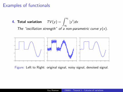
4. Total variation TV (y) =
∫ x1
x0
|y ′|dx
The “oscillation strength” of a non-parametric curve y(x).
0 2 4 6 8 10 12 14−1.5
−1
−0.5
0
0.5
1
1.5
0 2 4 6 8 10 12 14−1.5
−1
−0.5
0
0.5
1
1.5
0 2 4 6 8 10 12 14−1.5
−1
−0.5
0
0.5
1
1.5
Figure: Left to Right: original signal, noisy signal, denoised signal.
Guy Rosman 236861 - Tutorial 1 - Calculus of variations

The Euler-Lagrange Equation
Given the functional
f (u) =
∫ x1
x0
F(x , u(x), u′(x)
)dx
with F ∈ C3 and all admissible u(x) having fixed boundary valuesu(x0) = u0 and u(x1) = u1.
An extremum of f (u) satisfies the differential equation
Fu −d
dxFu′ = 0
with the boundary conditions u(x0) = u0 and u(x1) = u1.This equation is known as the Euler-Lagrange equation.
Guy Rosman 236861 - Tutorial 1 - Calculus of variations

The Euler-Lagrange Equation
Note: the second term of the equation does not have a parallel ina finite gradient expression from multivariate calculus – this term’sform expresses the relation of altering the value of u based on theeffect of its derivative. Later on we will see how this term stemsfrom the derivation of the E-L equation.
Guy Rosman 236861 - Tutorial 1 - Calculus of variations

The E-L equation (independent on u(x))
If the integrand does not depend on u(x),
f (u) =
∫ x1
x0
F(x , u′(x)
)dx ,
the E-L equation becomes a first-order differential equation
d
dxFu′ = 0
or
Fu′ = const.
Guy Rosman 236861 - Tutorial 1 - Calculus of variations

The E-L equation (independent on u′(x))
If the integrand does not depend on u′(x),
f (u) =
∫ x1
x0
F (x , u(x)) dx ,
the E-L equation becomes an algebraic equation
Fu(x , u(x)) = 0.
Guy Rosman 236861 - Tutorial 1 - Calculus of variations

The E-L equation (high-order functionals)
Given the functional
f (u) =
∫ x1
x0
F(x , u(x), u′(x), ..., u(n)(x)
)dx
with F ∈ Cn+2 and fixed boundary values u(i)(x0) = u(i)0 and
u(i)(x1) = u(i)1 for i = 0, ..., n − 1.
The Euler-Lagrange equation (also known as the Euler-Poissonequation) is
Fu −d
dxFu′ +
d2
dx2Fu′′ + (−1)n
dn
dxnFu(n) = 0.
Guy Rosman 236861 - Tutorial 1 - Calculus of variations

The E-L equation (multiple independent variables)
Given the functional
f (u) =
∫ΩF (x , u(x), ux1(x), ..., uxn(x)) dx
with x ∈ Rn and u|∂Ω = u∂Ω.
An extremum of f (u) satisfies the differential equation
∂F
∂u− d
dx1
∂F
∂ux1− ...− d
dxn
∂F
∂uxn= 0
with the boundary condition u|∂Ω = u∂Ω.
Guy Rosman 236861 - Tutorial 1 - Calculus of variations

The E-L equation (multiple functions)
Given the functional
f (u) =
∫ x1
x0
F(x , u1(x), ..., un(x), u
′1(x), ..., u
′n(x)
)dx
with F ∈ C3 and all admissible u(x) having fixed boundary valuesui (x0) = u0i and ui (x1) = u1i .
An extremum of f (u) satisfies the system of differential equations
Fui −d
dxFu′i = 0
with the boundary conditions u(x0) = u0 and u(x1) = u1.
Guy Rosman 236861 - Tutorial 1 - Calculus of variations
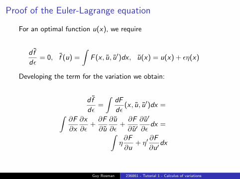
Proof of the Euler-Lagrange equation
For an optimal function u(x), we require
df
dε= 0, f (u) =
∫F (x , u, u′)dx , u(x) = u(x) + εη(x)
Developing the term for the variation we obtain:
df
dε=
∫dF
dε(x , u, u′)dx =∫
∂F
∂x
∂x
∂ε+
∂F
∂u
∂u
∂ε+
∂F
∂u′∂u′
∂εdx =∫
η∂F
∂u+ η′
∂F
∂u′dx
Guy Rosman 236861 - Tutorial 1 - Calculus of variations

Using integration by parts, we obtain: And hence,∫η∂F
∂u+ η′
∂F
∂u′dx =∫
η
(∂F
∂u− d
dx
∂F
∂u′
)dx +
[η∂F
∂u′
]x1x0
Since this equation should take place for every η, and assuming theboundary term cancels out, we obtain the E-L equation:
∂F
∂u− d
dx
∂F
∂u′= 0
Guy Rosman 236861 - Tutorial 1 - Calculus of variations

Problem 1: Minimum distance on a plane
Prove that the family of curves minimizing the distance
L =
∫ 1
−1
√1 + y ′2dx , y(−1) = a, y(1) = b
in the plane are straight lines.
−1.5 −1 −0.5 0 0.5 1 1.50.5
1
1.5
2
(−1,a)
(1,b)
Guy Rosman 236861 - Tutorial 1 - Calculus of variations

Problem 1: Minimum distance on a plane (cont.)
SolutionThe Euler-Lagrange equation
0 =d
dxFy ′ − Fy =
d
dx
(y ′√
1 + y ′2
).
Integration w.r.t. x yields
y ′√1 + y ′2
= γ = const.
Guy Rosman 236861 - Tutorial 1 - Calculus of variations
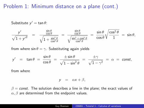
Problem 1: Minimum distance on a plane (cont.)
Substitute y ′ = tan θ:
y ′√1 + y ′2
=sin θcos θ√
1 + sin2 θcos2 θ
=sin θcos θ√
sin2 +cos2 θcos2 θ
=sin θ
cos θ
√cos2 θ
1= sin θ,
from where sin θ = γ. Substituting again yields
y ′ = tan θ =sin θ
cos θ=
± sin θ√1− sin2 θ
=±γ√1− γ2
= α = const,
from where
y = αx + β,
β = const. The solution describes a line in the plane; the exact values ofα, β are determined from the endpoint values.
Guy Rosman 236861 - Tutorial 1 - Calculus of variations

Problem 2: Heat Equation
We would like to minimize:∫Ω|∇u|2 =
∫Ω(u2x + u2y )dΩ
The Euler-Lagrange equation is:
EL(u) =d
dx(Fux ) +
d
dy
(Fuy)
=d
dx(2ux) +
d
dy(2uy )
= 2div (∇u)
= 2∆u
A gradient descent of the functional can be described as
ut = EL(u) = 2∆u
Guy Rosman 236861 - Tutorial 1 - Calculus of variations
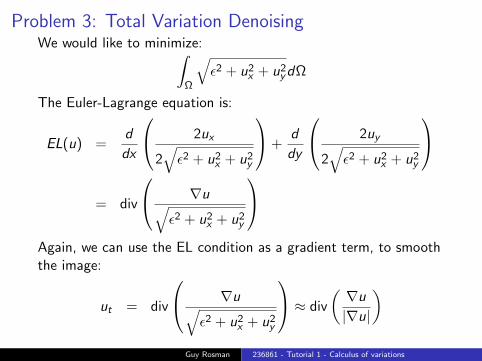
Problem 3: Total Variation DenoisingWe would like to minimize:∫
Ω
√ε2 + u2x + u2ydΩ
The Euler-Lagrange equation is:
EL(u) =d
dx
2ux
2√
ε2 + u2x + u2y
+d
dy
2uy
2√
ε2 + u2x + u2y
= div
∇u√ε2 + u2x + u2y
Again, we can use the EL condition as a gradient term, to smooththe image:
ut = div
∇u√ε2 + u2x + u2y
≈ div
(∇u
|∇u|
)Guy Rosman 236861 - Tutorial 1 - Calculus of variations
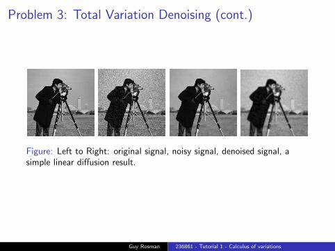
Problem 3: Total Variation Denoising (cont.)
Figure: Left to Right: original signal, noisy signal, denoised signal, asimple linear diffusion result.
Guy Rosman 236861 - Tutorial 1 - Calculus of variations
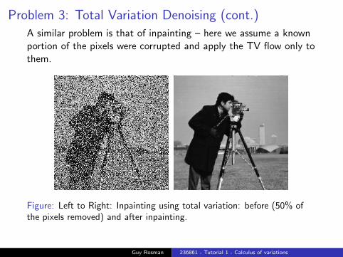
Problem 3: Total Variation Denoising (cont.)A similar problem is that of inpainting – here we assume a knownportion of the pixels were corrupted and apply the TV flow only tothem.
Figure: Left to Right: Inpainting using total variation: before (50% ofthe pixels removed) and after inpainting.
Guy Rosman 236861 - Tutorial 1 - Calculus of variations


![OSPF Security Project - webcourse.cs.technion.ac.ilwebcourse.cs.technion.ac.il/.../ho/WCFiles/2009-2-ospf-report.pdf · [2010] OSPF Security Project Michael Sudkovitch and David I](https://img.pdfslide.us/doc/110x75/5ae5b1dc7f8b9a6d4f8b9d9a/ospf-security-project-2010-ospf-security-project-michael-sudkovitch-and-david.jpg)