Brussels School of Engineering

Ecole polytechnique de Bruxelles Academic Year 2016-2017

Laboratory Notes

“Turbomachinery”

Aero-Thermo-Mechanics Department

Teaching Assistants : Laurent IppolitiJoelle Vincke

Chapter 1

Testing of a submersiblemotor-pump group

1.1 Purpose of the experiment

The determination of the operating characteristics of a submersible motor-pumpgroup, and more specifically the examination of the impact of the volume flow rate“qv” on the following parameters :

• the transferred useful specific energy “e”;

• the power consumed by the motor “Pmot”;

• the efficiency of the pump “ηp”;

• the rotational speed “N”.

1.2 Description of the set-up

1.2.1 The motor-pump group

The studied motor-pump group incorporates a vertical axis multicellular pump.The motor-pump group general dimensions are a diameter of 96 mm and a height of344 mm. Practically, this type of machine is used to drain water from narrow wells.

The upper part of the group is the pump section. The water inlet is positionedhalfway of the motor-pump group casing. The outlet section is circular and orientedaxially, and is on the upper end. Submersible motor-pump groups are usually builtmodularly, i.e. a multi-stage configuration can be assembled using a cascade ofindividual stages allowing pumps to cope with variables well-depths.

The lower part of the group consists of the electrical motor drive. For this kindof application, one uses mostly induction motors of the squirrel cage type, of whichthe stator is sealed to allow underwater operation.

The submersible motor-pump group is suspended from the discharge piping.Thus, the latter bears the full weight of the motor-pump group. The weight of themoving parts and the axial thrust inside the pump are handled by a thrust block

1

Figure 1.1: Description of the set-up

placed on a spherical joint at the bottom of the machine. The thrust block is usuallyof the Michell type.

The submersible pump used for this experiment is made of of five identical stages,each one consisting of a narrow, purely centrifugal rotor, a vaned diffuser and outletchannels preventing vortex formation at the entrance of the following stage.

Figure 1.2 shows the internal of a similar pump (number of stages differs).

1.2.2 The experimental set-up

The motor-pump group studied is immersed in a two-meter-deep reservoir. The inletof the pump is placed roughly 50 cm below the water surface. On the discharge sidethe following elements are placed:

• an obstruction flowmeter;

• a flow regulating valve “V 1”;

• a tank “R” used to recover the water from the pump with an overflow “TF”to send the water back to the reservoir.

1.3 Measuring devices

1.3.1 The electrical power

The power “Pmot” consumed by the group can be deduced using the current (“Imot”)measured by a ammeter placed over the electric leads. The motor is powered by

2

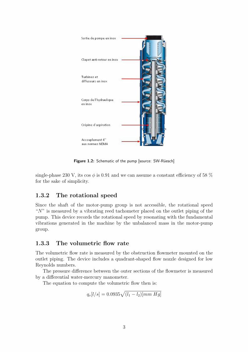
Figure 1.2: Schematic of the pump [source: SW-Ruesch]

single-phase 230 V, its cos φ is 0.91 and we can assume a constant efficiency of 58 %for the sake of simplicity.

1.3.2 The rotational speed

Since the shaft of the motor-pump group is not accessible, the rotational speed“N” is measured by a vibrating reed tachometer placed on the outlet piping of thepump. This device records the rotational speed by resonating with the fundamentalvibrations generated in the machine by the unbalanced mass in the motor-pumpgroup.

1.3.3 The volumetric flow rate

The volumetric flow rate is measured by the obstruction flowmeter mounted on theoutlet piping. The device includes a quadrant-shaped flow nozzle designed for lowReynolds numbers.

The pressure difference between the outer sections of the flowmeter is measuredby a differential water-mercury manometer.

The equation to compute the volumetric flow then is:

qv[l/s] = 0.0935√

(l1 − l2)[mm Hg]

3

1.3.4 Determination of the transferred useful specific en-ergy

We assume that the outlet section of the pump coincides with the inlet section ofthe flowmeter (“z3 = z0”). Also, one may prove that the depth below the watersurface where the inlet of the pump is found (“z0”) is of no importance.

The static part of the transferred useful specific energy “e” of the pump can bededuced knowing the effective pressure thanks to the manometer connected to theoutlet section (Bourdon pressure gauge placed at a height “zmr” above the watersurface of the well, see Figure 1.1). It can be shown that if “pr” is the effectivepressure indicated on the gauge, we have:(pout − pin

ρ

)+ g(zout − zin) =

prρ

+ gzmr

The height “zmr” of the manometer must be measured with a yardstick availablein the laboratory. It must be reminded that it is the base of the manometer thatmust be compared with the water surface.

The dynamic part of “e”, i.e. v2s2

, is deduced from the volume flow rate knowingthat the outlet piping has a diameter of 35 mm at the exit section.

1.4 Procedures

1.4.1 Preliminary checks

Before starting the motor-pump group, the following must be checked:

1. the valve “V 1” is open;

2. the communicating valve between the columns of the manometer is open, toavoid blowing the mercury out of the manometer.

1.4.2 Starting up

The motor-pump group will be started the first time in the presence of the assistant.

1. To avoid working with no flow, which could damage the pump because theheat from the mechanical losses are not evacuated, a sufficient flow rate needsto be selected opening valve “V 1”;

2. Using the push button on the control box, start the pump;

3. Close the communication valve of the differential manometer, to make themanometer functional.

4

1.4.3 Measurement of the motor-pump group characteris-tics

The operating characteristics of the motor-pump group will be established exper-imentally. For this purpose, several volume flow rates, needs to be selected usingvalve “V 1”. Care must be taken:

1. to explore the operating zone at significantly low flow rates;

2. to spread the flow rate measurements evenly while relying on the pressureindication read from the manometer to position the valve (without reachingpressure over 5 bar).

For each established operating regime, the following measurements must be made:

1. the heights “l1” and “l2” on the water-mercury manometer;

2. the pressure “pr” indicated by the Bourdon pressure gauge;

3. the current “Imot” on the ammeter;

4. the rotational speed “N” on the tachometer.

An additional operating point at no flow will be plotted. To avoid working with noflow, the values to use are provided:

• pressure: 5.4 bar

• current: 2.28 A

• rotational speed: 2980 rpm

1.5 Calculation and presentation of the results

1.5.1 Assignment

Demonstrate the equation described in the section 1.3.4.

1.5.2 Graphical results

Establish a single graph containing the transferred useful specific energy, mechanicalpower, efficiency and speed characteristics of the studied motor-pump group. Caremust be taken to choose the appropriate scale related to the measuring devices used.Result must be discussed.

5

Chapter 2

Testing of an axial-flow fan

2.1 Purpose of the experiment

For an axial-flow pressure fan with diffuser vanes, establish the dependency of:

• the transferred useful specific energy “e”;

• the effective power “Pe”;

• the efficiency “η”;

as a function of volumetric flow “qv” for a constant rotational speed “N”.

2.2 Theoretical aspects

2.2.1 Introduction

Axial fans are designed for high flow rates and relatively low pressure rises. Hence,like axial pumps, they are characterized by a high velocity coefficient.

Generally, three fundamental types of fans can be found depending on the ele-ments of which it is made. There is:

1. the single rotor configuration;

2. the rotor with inlet guide vanes configuration;

3. the rotor with outlet guide vanes configuration.

The latter two configurations, have the advantage of conserving the general di-rection of the flow, i.e. purely axial upstream and downstream, which is not the casewith a single rotor configuration.

2.2.2 Velocity triangle and shape of the vanes

We consider only the case of an axial fan made of a rotor followed by stator vanes,since this configuration is installed in the laboratory and needs to be examined. Thetest-setup incorporates the following elements :

6

Figure 2.1: Velocity triangle

• an intake;

• a rotor;

• a stator;

• an outlet diffuser.

To select the shape of the rotor vanes and the stator vanes, we will consider aradius “r” of the machine and draw the velocity triangle at the inlet and the outletof the rotor and combine them on a single figure. The velocity diagram is based thefollowing assumptions:

1. the machine being axial, we have equality of the rotational velocity at the inletand the outlet of the rotor, hence we have “u1 = u2 = ω r”;

2. the inlet and outlet areas of the rotor are also equal; moreover, if we suppose aconstant density “ρ” of the ventilated flow, which is reasonable because of thevery low pressure variations in axial-flow fans, conservation of mass then leadsto a constant volumetric flow causing the entering and exiting meridional flowspeeds to be equal;

3. at the inlet of the rotor, the absolute speed “c1” is axial and therefore per-pendicular to the rotational velocity “u1”; consequently the direction of therelative velocity “w1” defines an angle “β1”;

4. at the outlet of the rotor, as indicated in Euler’s formula1, the absolute velocity“c2” must have a tangential component “cu2 = c2 cosα2” aligned with therotational velocity, if we want the machine to be a compressor; in this case therelative velocity at the exit “w2” sets an angle β2 < β1.

For the losses to be minimal, the flow entering the impeller blades or the statorvanes should be “shockless”. This means :

1. for the rotor vanes of which the profile generally resembles an airfoil, the rela-tive speed is tangent to the leading edge and trailing edge camberlines of theimpeller blades, i.e. : “β1 = βr1”, “β2 = βr2”;

1e = u2cu2 − u1cu1 where “e” is the useful specific energy received or provided by the turbo-machine and “cu” is the component tangential to the absolute velocity.

7

2. for the stator vanes of which the profile generally resembles the one foundwith folded sheets, the absolute speed is tangent to the stator leading edgecamberline, i.e. “α2 = α2D”. Since the purpose of the vanes is to redirect theflow to the axial direction, the trailing edge angles are usually set to 90. Notethat in addition to the modification of the direction of the flow, the magnitudeof the speed is also reduced; the vanes work as a diffuser as well.

We can see also that the velocity triangle is only correct for one particular radius“r”. Indeed, for uniform inlet conditions, the velocity triangles will be a function ofradius “r” as for a given angular velocity, “u” will vary with “r” while ranging fromhub to tip. In other words, for minimum losses, the blades have to be twisted.

Finally we note that an axial fan without stator blades is inherently less effi-cient since the angular kinetic energy (whirl) in the flow leaving the compressor isdissipated by turbulent diffusion and is not recuperated to create pressure energy.Therefore, vaneless axial fans are only used for low power applications, such as thosefound in air conditioning systems, which demand really low pressure variations.

2.2.3 Pressure and velocity diagrams

We will focus on the axial variation of the following quantities:

• the static pressure “p”;

• the absolute velocity “c”;

• the total pressure “pt”.

Concerning the total pressure, we may recall that by definition, this pressure isequal to the pressure that would be obtained in a flow after bringing it isentropicallyand adiabatically to a standstill; therefore we have for an incompressible flow :

pt = p+ ρc2

2

We can note also that in a flow without energy sources and losses, as shown byBernoulli’s equation, the total pressure is conserved.

The lossless hypothesis discussed above may be applied to the experiment underexamination. Then one may observe that :

1. in the intake, the kinetic energy rises and thus the static pressure decreases;this happens without energy input, the total pressure is therefore conserved;

2. in the rotor, the machine being a compressor, there is an increase in pressureenergy; as seen on the velocity triangle, the exiting velocity “c2” is higher thanthe entering velocity “c1”; thus there is also an increase in kinetic energy andtherefore an increase in total pressure “pt”, this growth clearly indicates theenergy input from the rotor.

3. in the guide vanes, the velocity decreases because the diffuser outlet velocity“c3” is equal to the velocity “c1”; there is therefore a transformation of kineticenergy to pressure energy, the total pressure remaining the same since thereis no input of energy;

8

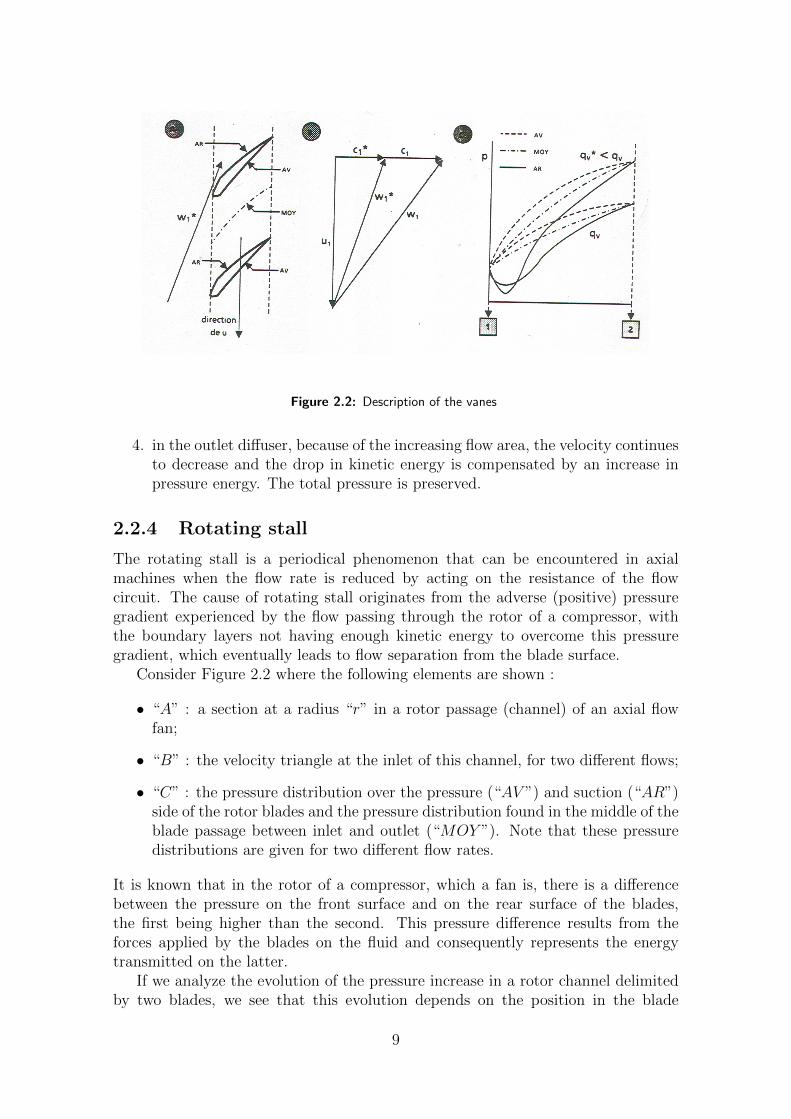
Figure 2.2: Description of the vanes

4. in the outlet diffuser, because of the increasing flow area, the velocity continuesto decrease and the drop in kinetic energy is compensated by an increase inpressure energy. The total pressure is preserved.

2.2.4 Rotating stall

The rotating stall is a periodical phenomenon that can be encountered in axialmachines when the flow rate is reduced by acting on the resistance of the flowcircuit. The cause of rotating stall originates from the adverse (positive) pressuregradient experienced by the flow passing through the rotor of a compressor, withthe boundary layers not having enough kinetic energy to overcome this pressuregradient, which eventually leads to flow separation from the blade surface.

Consider Figure 2.2 where the following elements are shown :

• “A” : a section at a radius “r” in a rotor passage (channel) of an axial flowfan;

• “B” : the velocity triangle at the inlet of this channel, for two different flows;

• “C” : the pressure distribution over the pressure (“AV ”) and suction (“AR”)side of the rotor blades and the pressure distribution found in the middle of theblade passage between inlet and outlet (“MOY ”). Note that these pressuredistributions are given for two different flow rates.

It is known that in the rotor of a compressor, which a fan is, there is a differencebetween the pressure on the front surface and on the rear surface of the blades,the first being higher than the second. This pressure difference results from theforces applied by the blades on the fluid and consequently represents the energytransmitted on the latter.

If we analyze the evolution of the pressure increase in a rotor channel delimitedby two blades, we see that this evolution depends on the position in the blade

9

passage, i.e. the evolution of the pressure on the suction side differs from thoseon the pressure side and in the middle of the channel. Indeed if on the intradossurface there is a slight overpressure with respect to the midline, on the other handon the extrados surface there is a slight underpressure with respect to the midline.Moreover, on extrados there is also a zone of strong underpressure near the inletsection (leading edge) because of the reduced flow area. Consequently, the pressuregradient is always higher on the suction side of the blade, which therefore makes itmost susceptible to rotating stall.

When the flow rate is reduced by augmenting the resistance of the outlet piping,the following observations can be made:

1. the relative velocity at the inlet is deflected and the angle of attack of theblades increases consequently;

2. due to the growth in angle of attack, the pressure on the extrados drops evenfurther while the low pressure zone gets more difficulty reached by the flowand is subject to a “jet effect”;

3. the outlet pressure increases with the resistance of the circuit.

As Figure 2.2 indicates, the pressure gradient on the extrados of the blades increasesfor a double reason. If the flow rate is too much reduced, the boundary layerenergy will not be sufficient and the boundary layer will abruptly separate from theextrados. In an axial-flow machine, this separation does not occur simultaneouslyon all blades. Note that any dissymmetry of the flow, even caused by the verygeometric layout of the machine may be sufficient to cause flow separation on oneor more successive blades.

The separated zones in a blade passage increase the flow resistance, in turnreducing the flow rate through the passage significantly. Consequently a part of theflow that should have flown through the channel with separation is now divertedto the adjacent channels. The following blade in the direction of rotation has itsangle of attack reduced while the previous vane has an increased angle of attack.The latter blade will then undergo flow separation as well. While on the other sidewhere the vane induced the initial separation, the situation improves because theboundary layer will reattach. Clearly, the stall zone, where the flow is separated, willmove in the rotor. Hence, the separation phenomenon is given the name “rotatingstall”.

The angular velocity “ωDr” of this rotating stall moves upward in the rotor,though in absolute terms, rotating stall rotates in the same direction as the rotor,but at a reduced angular speed “ω” of the rotor. This means that for an observerfixed on the rotor, the rotating stall “goes up” the rotor, in absolute, the phenomenonrotates in the same direction than the rotor but at a reduced speed “ωD”.

The rotational stall therefore introduces a new characteristic frequency of themachine that should be taken in account when sizing the blades. The resonancefrequency of the blades should not coincide with the frequency of the rotating stallphenomenon. Otherwise, the machine could be seriously damaged.

Depending on the height en geometry of the blades, the rotating stall will appearonly on a part of the blade or abruptly, from the from the root to the tip of the

10

blades. In the first case,a continuously decreasing flow rate will result in a stalledarea that progressively grows in radial and tangential directions. In the secondcase,the stall region grows only in the tangential direction. Note that a distinctioncan be made between a stall area that grows gradually from hub to tip and a stallarea formed instantly affecting the complete blade area from hub to tip.

We will only consider the properties of the sudden rotating stall which occurs inaxial-flow machines with relatively short blades, as this is the case for the fan usedfor the experiment. These properties are:

1. starting from the normal flow and with an decreasing flow rate, the rotat-ing stall appears suddenly and there will be a discontinuity in the energeticcharacteristic;

2. starting from the perturbed flow and with an increasing flow rate, the rotatingstall disappears again suddenly and the energetic characteristic will displayanother discontinuity;

3. the phenomenon shows an hysteresis, the rotating stall appears for a decreasingflow rate at a lower flow rate than the flow rate for which the rotating stalldisappears for an increasing flow rate;

4. when it appears, the zone in stall can be a unique sector, which is the case forthe fan in this experiment, or different sectors symmetrically positioned;

5. during the tangential propagation of the rotating stall occurring at decreasingflow rate, the useful specific energy decreases only slightly, the situation beingsimilar to reducing the section available for the fluid.

2.2.5 Working with backflow

When the rotating stall is affecting the complete flow area and if the resistance ofthe circuit continues to be increased, a new regime will be established, the backflowcondition or reverse flow.

On the root of the blades, the transferred energy is not sufficient anymore toensure a positive flow rate. Only the periphery of the blades is still sufficientlyeffective. Hence, only in the outer blade region a positive flow can be achieved anda part of the flow returns to the inlet via the inner blade regions (backflow).

At a decreasing flow rate, the backflow continues to decrease and at no flow,there is still an intense flow in the rotor because the rotor still delivers high specificenergy to the fluid, thus also a significant amount of power. It is also at no flowthat axial-flow machines consume their maximal power. To conclude, note thatthe transition from the rotating stall condition to the backflow condition presents asmall discontinuity.

2.2.6 The reduced variable for an axial-flow machine

In the case of an axial-flow machine, the definition of Rateau’s coefficients require theuse of a specific geometric variable to produce the reduced variables. By convention,

11

Figure 2.3: Description of the set-up

the RMS radius “rm” will be used for this purpose, which is computed from the radii“ri” and “re” at the root and the tip of the vanes, i.e.:

rm =

√r2e + r2i

2

2.3 Description of the set-up

2.3.1 The fan

The axial-flow fan used in this experiment is of the pressure type and it consists ofthe following elements, in stream-wise order :

• an inlet intake;

• a rotor with 14 blades;

• a stator with 17 vanes;

• an outlet diffuser;

Note that the number of rotor blades and stator vanes are prime to each otherto avoid resonance phenomena in the flow.

The direct current driving motor is placed in the air intake. It drives the rotordirectly, without any reduction. The maximum rotational speed of this machine is2500 rpm.

The main geometric dimensions are the following:radius at the root of the rotor vanes “ri” : 178 mmradius at the tip of the rotor vanes “re” : 280 mmdiameter of the outlet section “D” : 400 mm

12

2.3.2 The flow network setup

The flow network consists of the following elements:

1. a piping of which the length and the diameter are respectively 4.30 m and0.4 m and in which a honeycomb grid straightens the flow;

2. a divergent duct for connection;

3. an obstructing flowmeter in which the measuring element is a nozzle with adiameter of 0.6 m;

4. a motorized cone for flow control.

2.3.3 Electrical supply of the set-up

The motor driving the fan has an independent constant excitation. The rotationalspeed is obtained by setting the voltage “U” at the terminals of the rotor, a voltageproduced by a rectifier.

2.4 Measuring devices

2.4.1 Atmospheric conditions

The atmospheric conditions will be measured (with a Fortin barometer providedin the room where the fan test set-up is placed) and calculated. Particularly, thedensity of ambient air “ρatm” will be deduced, and it will be assumed that, given thelow pressure variations in the studied fan, this density is constant in the completeset-up. To be complete, the incompressibility hypothesis should be verified.

ρ = ρatm = constant

2.4.2 Rotational speed

The rotational speed of the fan is measured thanks to a tachometer with an elec-tromagnetic sensor; it records impulses from the rotation of a wheel with 60 teethfixed on the axis of the fan. A digital indicator shows the rotational speed in [rpm]on the control panel of the set-up.

2.4.3 The effective power of the fan

The effective power “Pe” of the fan is calculated from the electrical power “Pelec”consumed by the driving motor end by knowing the losses “Pp” in the motor:

Pe = Pelec − Pp

The power “Pelec” is given by the voltage “U” on the motor terminals and thecurrent “I” measured by respectively a voltmeter and an ampere-meter. They areindicated digitally on the control panel. The losses “Pp” of the motor are composed

13

by Joule dissipation “PJ”, losses on the brushes “Pb” and the sum of magnetic andmechanical losses “Pm+m”. To evaluate those losses, the following informations isavailable:

1. the rotor resistance is 0.325 Ω;

2. the voltage drop at the contact of the brush and the commutator is 2 V;

3. the sum of magnetic and mechanical losses can be computed in function of therotational speed “N” [rpm] and the voltage on the motor “U” [V] with thefollowing equation:

Pm+m[W ] = 2.85 · 10−3U2 − 5 · 10−7NU2 + 2.3 · 10−5N2 + 15

2.4.4 Flow rate

It was already mentioned earlier in the text that the flow rate is measured by anobstruction flowmeter with a nozzle. The characteristics of the nozzle are the fol-lowing:

flow coefficient : α = 1.142throat diameter : d = 464.5 mm

Provided that the flow is incompressible, the equation for the mass flow rate thenis:

qm = α ε Sc

√2 · ∆p · ρ (2.1)

where “Sc” is the throat section of the flowmeter, “ρ” is the density of the fluidcalculated using the conditions ruling upstream the flow meter (use the upstreampressure measurement) and “qm” is the mass flow in the flowmeter.

The pressure drop “∆p” over the flowmeter is measured in [mbar] thanks toa differential manometer. Since the change in recorded pressure is small, we canassume here that:

1. the discharge coefficient “ε” is equal to one;

2. the density of air upstream of the flowmeter remains constant and equal tothe density of ambient air.

2.4.5 Useful specific energies

In the present case, given that the fan is of the pressure type while assuming aconstant air density, it is found that :

e =p4 − patmρatm

+c242

+ (ef )3−4

The measurement section “4” is found in the outlet piping 4 m downstream theoutlet “3” of the fan. Taking the honeycomb grid in the inlet piping and the surfaceroughness into account, one may assume that, while neglecting the influence of theReynolds number :

(ef )3−4 = 0.40c242

14

The section “4” is equipped with a differential mechanical manometer that measuresthe pressure difference “p4−patm” directly in [mbar]. An offset may have to be addedor subtracted.

2.5 Procedure

2.5.1 Planning of the experiment

Due to the large amount of experimental data that needs to be processed in a re-stricted time span, it is recommended to prepare a computer program (e.g. spread-sheet) for this purpose. The following input and output data are to be analyzed :

Inputs

• density of ambient air “ρatm” [ kgm3 ];

• pressure difference on the flowmeter “∆p” [mbar];

• outlet pressure “p4 − patm” [mbar];

• rotational speed “N” [rpm];

• voltage on the motor “U” [V ];

• rotor current in the motor “I” [A].

Outputs

• volumetric flow rate “qv” [m3

s];

• useful specific energy “e” [ Jkg

];

• effective power “Pe” [kW ];

• efficiency “η” [−].

2.5.2 Measurement of fan characteristics at constant rota-tional speed

The working characteristics of the fan will be determined for a rotation speed of2000 rpm. It is advised to proceed in the following manner:

1. firstly, measure the working point concurring with the maximum flow rate.

2. Secondly, decrease the flow rate progressively to the minimum attainable valueby moving the regulating cone, disregarding the occurrence of rotating stallwhich is recognizable by its characteristic sound. Distribute the working pointsevenly based on “∆p” measured over the flow meter and which is indicateddigitally on the control panel. It is suggested to reduce the flow stepwiseapplying a consecutive reduction of 0.1 (0.05 below 0.7) on “∆p” in order togain sufficient measurements.

15

3. Finally, by selecting the position of the flow regulating cone, the flow rateincrease progressively returning to the initial condition.

2.6 Calculation and presentation of the results

2.6.1 Characteristics at constant rotational speed

The results of the closing and opening of the cone must be plotted in a singlegraph as a function of volumetric flow rate “qv”. Care must be taken to choosethe appropriate scale when plotting the results, depending on the precision of themeasuring devices used. It is advised to put the origins of those scales on the graph.

16